Economic Policy Uncertainty and the Yield Curve∗
Markus Leippold† Felix H. A. Matthys‡
October 30, 2015
Abstract
We study the impact of economic policy uncertainty on the term structure of nominal interest
rates. We develop a general equilibrium model, in which the real side of the economy is driven by
government policy uncertainty and the central bank sets money supply endogenously following a
Taylor rule. We analyze the impact of government and monetary policy uncertainty on nominal
yields, short rates, bond risk premia, and the term structure of bond yield volatility. Our affine
yield curve model is able to capture both the shape of the interest rate term structure as well as
the hump-shape of bond yield volatilities. Our empirical analysis shows that higher government
policy uncertainty leads to a decline in yields and an increase in bond yield volatility, whereas
monetary policy uncertainty has no significant contemporaneous effect on yields nor volatilities.
However, it is an important predictor for bond risk premia.
JEL classification: G01, G12, G14, G18
Key Words: Term structure modeling, yield volatility curve, policy uncertainty, bond risk premia
∗This paper benefited greatly from discussions with Yacine Aıt-Sahalia, Caio Almeida, Markus Brunnermeier,Jerome Detemple, Itamar Drechsler, Darell Duffie, Fabio Trojani, Valentin Haddad, Oleg Itskhoki, Jakub Jurek,Philippe Mueller, Jean-Charles Rochet, Christopher Sims, David Srear, Adi Sunderam, Josef Teichmann, and WeiXiong. For helpful comments we would like to thank the seminar participants of the 2015 SAFE Asset PricingWorkshop in Frankfurt, the Finance and Math Seminar ETH and University of Zurich, the 12th Doctorial Workshop inFinance at Gerzensee, the Princeton Student Research Workshop, Financial Mathematics Seminar at ORFE PrincetonUniversity, Bank of England, Central Bank of Mexico, and ITAM. Financial support from the Swiss Finance Institute(SFI), Bank Vontobel, the Swiss National Science Foundation and the National Center of Competence in Research“Financial Valuation and Risk Management” is gratefully acknowledged.†Swiss Finance Institute (SFI) and University of Zurich, Department of Banking and Finance, Plattenstrasse 14,
8032 Zurich, Switzerland; [email protected].‡Princeton University, Bendheim Center For Finance; [email protected].
1 Introduction
Economic policy is driven by government and central banking actions. Governments define fiscal
policy and impose regulations, while central banks manage the money supply and set nominal short
rates. These policies have a fundamental impact on financial markets. However, despite good
intentions their effectiveness remains uncertain at best. In this paper, we explore the impact of such
policy uncertainty on the term structure of interest rates, its corresponding volatility curve, and on
bond risk premia. We develop a general equilibrium model, in which the real side of the economy
is subject to government policy uncertainty and the nominal side of the economy is affected by
monetary policy shocks. Our model setup allows us to derive an approximate analytical solution for
the general equilibrium in the case where the representative agents has CRRA-utility. A key model
device is the assumption of the central bank following a Taylor rule, which links the real with the
nominal side of the economy and turns out to be crucial in reproducing the salient features of the
nominal term structure and its volatility curve.
Our general equilibrium framework builds upon Buraschi & Jiltsov (2005). However, the key
distinction is that for our representative agent we depart from the log-utility assumption and impose
a constant relative risk aversion (CRRA) utility. It is well known that for such a utility specification,
no closed-form solution for the term structure of interest rates can be obtained. Using perturbation
methods, we find that the agents’ optimal controls remain affine in the state variables up to a first
order approximation in the risk aversion coefficient. This result allows us to study the effect of
changing risk aversion on the term structure of interest rates and the yield volatility curve, which
previous papers such as Buraschi & Jiltsov (2005) or Ulrich (2013) were not able to do, and which
turn out to be non-trivial.
In our model, both government and monetary policy uncertainty are affecting nominal yields, the
term structure of volatility, and bond risk premia in a fundamentally different way. An increase in
government policy uncertainty adversely affects the trend component of real output growth. There-
fore, it renders capital investments more risky, which will eventually induce investors to favor safe
assets such as government bonds. Such a flight-to-quality behavior will raise government bond
prices and therefore drives down its yields. This observation is in line with Bloom (2009), who
1
argues that productivity growth falls, because higher uncertainty causes firms to temporarily pause
their investment. Moreover, in our model economy higher government policy uncertainty will not
only negatively affect the long run growth path of production. It also increases its volatility and
therefore leads to a worsening of economic growth prospects, which are fundamental to the agents
consumption-investment allocation problem.1
Not only does government policy uncertainty play an important role in determining the level of
interest rates, but it has also a crucial impact on the level and shape of the term structure of bond
yield volatilities. Although our model belongs to the class of affine models as introduced by Duffie &
Kan (1996), we can replicate the typical hump-shape of the volatility term structure, caused by the
empirical observation that volatility tends to be highest around the two-year maturity bucket. The
key mechanism leading to this result is that government policy uncertainty negatively affects the long
run growth path of productivity, which translates into a hump-shaped curve at a higher volatility
level. With this amplification mechanism we can also explain the ‘excess bond yield volatility puzzle’
that empirical bond yields, especially at the long end of the term structure, cannot be reproduced
by standard affine models of the term structure of interest rates (see Shiller (1979) and Piazzesi &
Schneider (2006)).2
Dealing wit policy uncertainty, a fundamental question that arises in this context is: What is
an appropriate measure for government and monetary policy uncertainty? As starting point, we use
the economic policy uncertainty (EPU) index developed by Baker et al. (2012). According to their
definition, the EPU index contains uncertainty related to both government and monetary policy.
Hence, we aggregate the corresponding EPU constituents into a government (GPU) and a monetary
policy uncertainty (MPU) index.
[Figure 1 about here]
1Our model is similar in style to the long run risk model of Bansal & Yaron (2004). However, the key distinctivedifference is that the long run growth component and the market price of output risk are both driven by the sameunderlying risk factor, namely government policy uncertainty. Furthermore, our setting can also be compared to theliterature on real business cycle analysis. For instance, shocks to trend growth exhibit fundamentally different effectson the (real) economy as opposed to transitory fluctuations. The agents or county’s reaction to temporary shocks is toborrow in the short run to smooth out consumption. However, if the shock is more persistent, the long run consumptionlevel has to be adjusted as borrowing for an infinite time horizon is not longer possible.
2A possible solution to this problem is to introduce heterogeneous agents who have different prior beliefs about somefundamental economic variable, such as for instance inflation as in Xiong & Yan (2010) or to introduce time-varyingrisk preference as in Buraschi & Jiltsov (2007), which are however analytically less tractable.
2

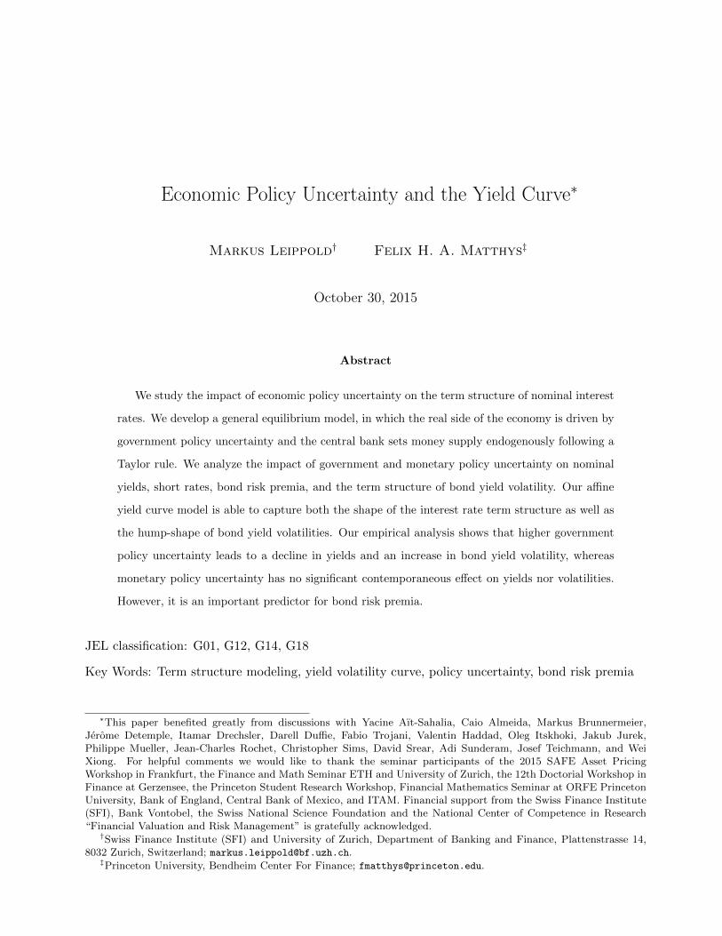
In Figure 1 we plot the relationship between U.S. treasury bond yields and volatilities together
with the EPU, GPU, and MPU index for the period of 1995 to 2014. The first two prominent spikes
of the EPU index are related to the terrorist attacks on the World Trade Center and the 2nd Gulf
War. By the end of 2003 and until the outbreak of the financial crisis in 2008, the US economy
entered a steady economic growth phase. Both, the EPU and GPU show similar patterns. They
declined in the pre-crisis period and started to peak at the onset of the financial crisis. The EPU
and GPU index remain at a high level ever since, exhibiting highly volatile behavior. In contrast, the
MPU index slowly reversed to its pre-crisis level. We attribute this observation to the fact that the
EPU and GPU index captures political uncertainty, which was especially high during the debt-ceiling
crisis of 2011 and lasted until late 2013 where some governmental authorities were even forced to
suspend their services temporarily.
Figure 1 also shows that both the EPU and GPU index exhibit a countercyclical pattern with
nominal yields. When the EPU or GPU index is high, yields tend to go down. This apparent negative
relationship is also confirmed by computing the sample correlation coefficient, which ranges from -
0.544 (EPU, 1 year) to -0.32 (GPU, 10 years) for the period January 1990 until June 2014.3 These
numbers suggest that higher economic or government policy uncertainty leads to lower treasury bond
yields. Thus, as political risk increases, investors seek safer assets and therefore start to shift from
stocks to (government) bonds, which is in line with the predictions in Pastor & Veronesi (2013).4
The discussion above suggests that government and monetary policy uncertainty may have dif-
ferent effects on yields and volatilities. Therefore, we not only split economic uncertainty into these
two different components, but we allow government policy uncertainty to play a role for interest rate
policy. The empirical analysis of the model confirms our theoretical prediction in that government
policy uncertainty is the main driver in contemporaneous movements in the term structure of interest
rates and its volatility curve.
3The time series correlation between the EPU and GPU (MPU) is 0.857 (0.657) and 0.572 between the GPU andMPU index. As can be inferred from Figure 1, the monetary policy uncertainty index appears to have no link withcontemporaneous movements in nominal yields. Indeed, the estimated time series correlation is roughly zero along theentire term structure. We collect the all empirical sample correlation of treasury bond yields and the EPU, GPU andMPU indexes in Table 6 as well as realized volatility and EPU, GPU and MPU indexes in Table 7 in Appendix B.Furthermore, the sample correlation between the EPU and the VIX index is 0.44 for the same period.
4Using also the EPU index of Baker et al. (2012), they show that political uncertainty raises not only the equityrisk premium but also the volatilities and correlations of stock returns.
3
There is increasing evidence that policy uncertainty leads to direct reactions of the central bank
authority (see for instance David & Veronesi (2014)). To motivate a link between government policy
uncertainty and yields for our model design, we estimate pairwise Vector Auto Regressions (VAR)
for the GPU and MPU with the three-month T-bill rate, which we take as proxy for monetary policy.
[Figure 2 about here]
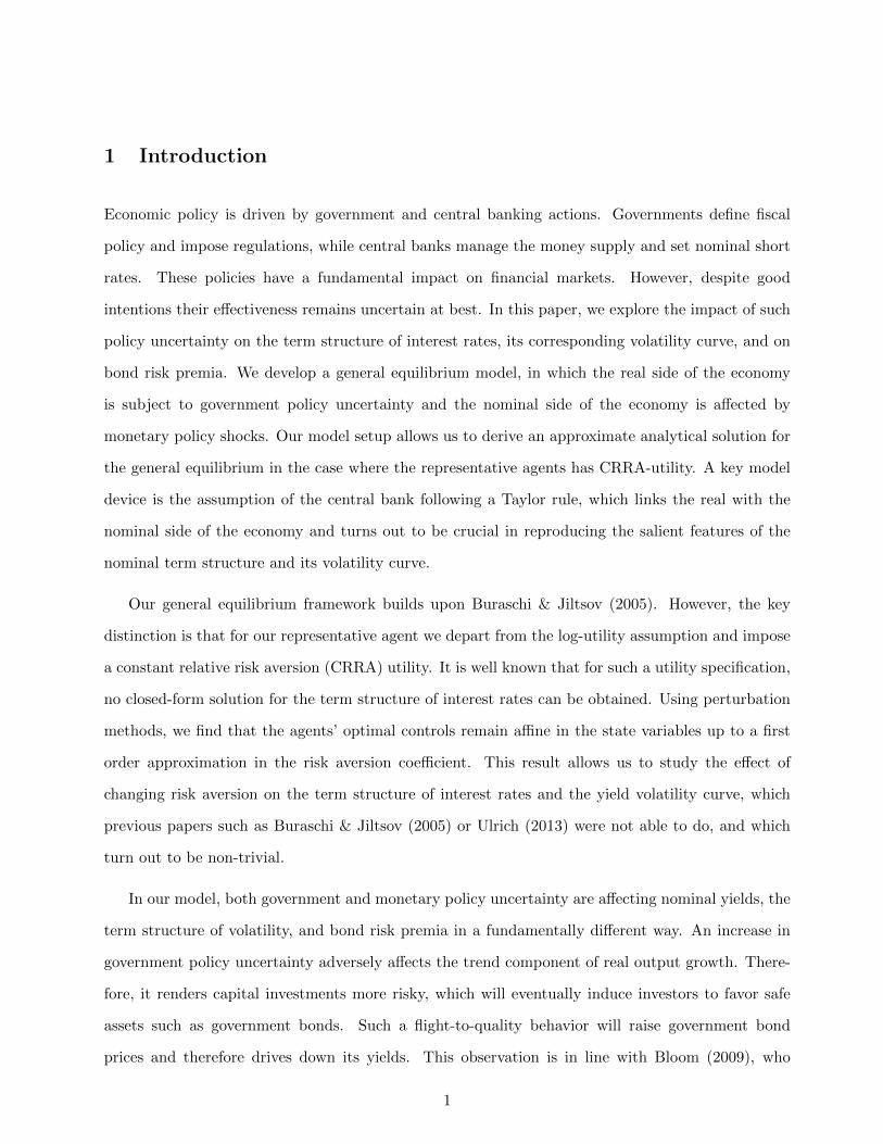
Figure 2 reports the resulting impulse responses for the time period from January 1995 to June
2014. Panel A reveals that a shock to the GPU index leads to a sustained negative impact on the
short-term rate and hence on future monetary policy. This impact remains highly significant up to
a time horizon of more than 20 months. In contrast, from Panel B we observe that a shock to the
short-term rate has no significant impact on the GPU index.5 This suggests that government policy
uncertainty shocks drives monetary policy actions, but not the other way around. Hence, the central
bank conducts its monetary policy taking into account uncertainty shocks from the real side whereas
the central banks interest rate policy does not seem to affect fiscal uncertainty.
We provide a theoretical explanation for the empirical results above. In our model economy,
higher real uncertainty lowers productivity growth, which feeds into the monetary policy through
our assumption that the central bank controls the money supply growth following a Taylor rule.
Hence, the monetary authority’s efforts to stabilize growth (and inflation) causes it to react to real
uncertainty by lowering the cost of capital. Moreover, since we assume money neutrality, nominal
shocks do not have an impact on the real side of the economy. However, the converse is not true.
The equilibrium price level growth is driven by the capital accumulation growth, which implies that
the nominal side is also driven by shocks from the real side, namely government policy shocks.
Through these two transmission channels, inflation and capital accumulation growth targeting, the
money supply growth becomes a function of government policy uncertainty. Therefore, by letting
the central bank react endogenously to deviations from long run capital growth and inflation targets
establishes an important link between the real and the nominal side of the economy that allows
5Further analyzing the impulse responses from our VAR model, we find that the MPU index has a similar behavioras the GPU index in that it does (negatively) influence monetary policy, but the MPU does not respond to a shock inthe short rate. Furthermore, the response of the short rate from a MPU shock is less pronounced than from a GPUshock. Finally, the MPU and GPU responses to GPU and MPU shocks are negligible and become insignificant afterfour to five months. We do not report these graphs here, but they can be obtained on request.
4
government policy shocks to affect nominal quantities. This link proves to be essential in order to
simultaneously match both the term structure of interest rates and its corresponding volatility curve.
Finally, we allow both monetary and government policy shocks to carry a risk premium. Hence,
our model accommodates a time-varying risk premia in bond returns, which implies that mone-
tary and government policy uncertainty are priced risk factors and the equilibrium inflation process
exhibits heteroskedastic time-variation in both variables.
While our paper belongs to the class of equilibrium finance models of the term structure, it is
specifically related to the following strands of literature.6 Traditional work on asset pricing usually
abstracts from modeling government uncertainty and its impact on asset prices. However, especially
since the European debt crisis starting in 2010 and the 2011 Congress debate about raising the
fiscal debt ceiling in the US, policy uncertainty has recently attracted interest from academia. For
instance, Pastor & Veronesi (2012) and Pastor & Veronesi (2013) develop a general equilibrium
model, in which the profitability of firms is driven by government policy, and discuss the impact of
policy risk on stock prices. Several empirical papers have shown that uncertainty about political
outcomes has a significant effect on asset returns and corporate decisions.7 There is also a large
strand of literature trying to infer political risk from government bond yields such as, e.g., Huang
et al. (2015) who empirically study the relationship between political risk and government bond
yields. For an overview of this literature, we refer to Bekaert et al. (2014).
While the literature on government policy impacts is sparse but growing, the fundamental link
between monetary policy and the term structure of interest rates and volatilities has been studies
6Equilibrium term structure models include, among many others, Wachter (2006), Piazzesi & Schneider (2006),Buraschi & Jiltsov (2007), Gallmeyer et al. (2007), Bekaert et al. (2009), and Bansal & Shaliastovich (2013). Recently,macro-finance term structure models have been critisized for their failure to accomodate for the presence of “unspannedmacroeconomic risk,” see Joslin, Priebsch & Singleton (2014). However, there is support for spanned macro-financeterm structure models. Basically, Bauer & Rudebusch (2015) claim to have resolved the unspanning puzzle. Althoughour model belongs to the spanned model class, we do not delve further into this discussion but refer the interestedreader to the two cited papers above.
7For instance, early studies include Rodrik (1991) or Pindyck & Solimano (1993). They show empirically thatuncertainty about political factors can lead to lower investment expenditures, especially when investment is irreversible.More recently, Durnev (2010) and Julio & Yook (2012) document that firms tend to withhold their investment activityprior to national elections. Gulen & Ion (2012) argue, based on the newly developed policy index by Baker et al.(2012), that policy uncertainty reduces firm and industry level investment and that the magnitude of reduction issubstantial. Boutchkova et al. (2012) take the analysis further and show that some industries are more sensitive topolitical uncertainty than others. Some further related articles analyzing the relationship between political uncertaintyand asset returns include Belo et al. (2013), Bialkowski et al. (2008) or Bond & Goldstein (2012).
5

more extensively. For the yield effects we refer to, e.g., Kuttner (2001), Piazzesi (2005), Fleming
& Piazzesi (2005), Gurkaynak et al. (2005a), and Wright (2012). For the volatility effects see, e.g.,
Balduzzi et al. (2001), Piazzesi (2005) or de Goeij & Marquering (2006), among others. The literature
on the link between monetary policy and bond risk premia is surveyed in Buraschi et al. (2014). In
an empirical study, they find that monetary shocks are indeed an important source of priced risk,
helping to explain the risk premia in bond markets. Using a standard predictability regression of
excess bond returns, they find that monetary policy shocks account for a substantial part of the
variance of bond excess returns, which is in line with our empirical results.
Despite the recent attention brought to modeling the impact of policy uncertainty on asset prices,
the papers mentioned above either address the empirical link between government bond yields and
policy uncertainty or focus on the theoretical impact that a given government policy has on stock
returns. Our paper provides a theoretical framework for studying the impact of both government and
monetary policy uncertainty on the nominal yield curve and its implications for the term structure
of bond yield volatility.
The reminder of the paper is organized as follows. Section 2 presents the model. Section 3
discusses the impact of government as well as monetary policy uncertainty on the term structure of
nominal interest rates, the yield volatility curve and the bond risk premium. Section 4 summarizes
our empirical results and Section 5 concludes.
2 The baseline model economy
Our model economy consists of a real and a monetary sector. For the real sector, we consider a
production economy with a representative agent producing a single good at a constant return-to-
scale production technology. As in Buraschi & Jiltsov (2005), real monetary holdings Mdt provide
a transaction service by reducing the total amount of gross resources required for a given level of
consumption Ct.
Assumption 1 (Preferences of Representative Agent). Let U(Xt) denote expected utility over the
real net consumption holdings X and β > 0 the subjective discount factor. The agent has constant
6
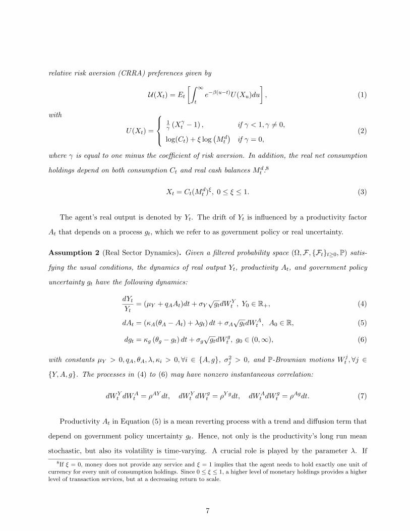
relative risk aversion (CRRA) preferences given by
U(Xt) = Et
[∫ ∞t
e−β(u−t)U(Xu)du
], (1)
with
U(Xt) =
1γ (Xγ
t − 1) , if γ < 1, γ 6= 0,
log(Ct) + ξ log(Mdt
)if γ = 0,
(2)
where γ is equal to one minus the coefficient of risk aversion. In addition, the real net consumption
holdings depend on both consumption Ct and real cash balances Mdt :8
Xt = Ct(Mdt )ξ, 0 ≤ ξ ≤ 1. (3)
The agent’s real output is denoted by Yt. The drift of Yt is influenced by a productivity factor
At that depends on a process gt, which we refer to as government policy or real uncertainty.
Assumption 2 (Real Sector Dynamics). Given a filtered probability space (Ω,F , Ftt≥0,P) satis-
fying the usual conditions, the dynamics of real output Yt, productivity At, and government policy
uncertainty gt have the following dynamics:
dYtYt
= (µY + qAAt)dt+ σY√gtdW
Yt , Y0 ∈ R+, (4)
dAt = (κA(θA −At) + λgt) dt+ σA√gtdW
At , A0 ∈ R, (5)
dgt = κg (θg − gt) dt+ σg√gtdW
gt , g0 ∈ (0,∞), (6)
with constants µY > 0, qA, θA, λ, κi > 0, ∀i ∈ A, g, σ2j > 0, and P-Brownian motions W j
t ,∀j ∈
Y,A, g. The processes in (4) to (6) may have nonzero instantaneous correlation:
dW Yt dW
At = ρAY dt, dW Y
t dWgt = ρY gdt, dWA
t dWgt = ρAgdt. (7)
Productivity At in Equation (5) is a mean reverting process with a trend and diffusion term that
depend on government policy uncertainty gt. Hence, not only is the productivity’s long run mean
stochastic, but also its volatility is time-varying. A crucial role is played by the parameter λ. If
8If ξ = 0, money does not provide any service and ξ = 1 implies that the agent needs to hold exactly one unit ofcurrency for every unit of consumption holdings. Since 0 ≤ ξ ≤ 1, a higher level of monetary holdings provides a higherlevel of transaction services, but at a decreasing return to scale.
7
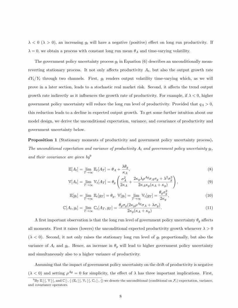
λ < 0 (λ > 0), an increasing gt will have a negative (positive) effect on long run productivity. If
λ = 0, we obtain a process with constant long run mean θA and time-varying volatility.
The government policy uncertainty process gt in Equation (6) describes an unconditionally mean-
reverting stationary process. It not only affects productivity At, but also the output growth rate
dYt/Yt through two channels. First, gt renders output volatility time-varying which, as we will
prove in a later section, leads to a stochastic real market risk. Second, it affects the trend output
growth rate indirectly as it influences the growth rate of productivity. For example, if λ < 0, higher
government policy uncertainty will reduce the long run level of productivity. Provided that qA > 0,
this reduction leads to a decline in expected output growth. To get some further intuition about our
model design, we derive the unconditional expectation, variance, and covariance of productivity and
government uncertainty below.
Proposition 1 (Stationary moments of productivity and government policy uncertainty process).
The unconditional expectation and variance of productivity At and government policy uncertainty gt,
and their covariance are given by9
E[At] = limT→∞
Et[AT ] = θA +λθgκA
, (8)
V[At] = limT→∞
Vt[AT ] = θg
(σ2A
2κA+
2κgλρAgσAσg + λ2σ2
g
2κAκg(κA + κg)
), (9)
E[gt] = limT→∞
Et[gT ] = θg, V[gt] = limT→∞
Vt[gT ] =θgσ
2g
2κg, (10)
C[At, gt] = limT→∞
Ct[AT , gT ] =θgσg(2κgρ
AgσA + λσg)
2κg(κA + κg). (11)
A first important observation is that the long run level of government policy uncertainty θg affects
all moments. First it raises (lowers) the unconditional expected productivity growth whenever λ > 0
(λ < 0). Second, it not only raises the stationary long run level of gt proportionally, but also the
variance of At and gt. Hence, an increase in θg will lead to higher government policy uncertainty
and simultaneously also to a higher variance of productivity.
Assuming that the impact of government policy uncertainty on the drift of productivity is negative
(λ < 0) and setting ρAg = 0 for simplicity, the effect of λ has three important implications. First,
9By E [·], V [·], and C [·, ·] (Et [·], Vt [·], Ct [·, ·]) we denote the unconditional (conditional on Ft) expectation, variance,and covariance operators.
8

it lowers expected growth of productivity proportionally to θg/κA. Second, it increases volatility of
At linearly. Lastly, it renders C[At, gt] negative, which will be of central importance to capture the
stylized facts of bond yield volatility within our model.
We can now proceed with the formulation of the agent’s capital budget constraint. Without loss
of generality, we use capital depreciation as the only cost component.10
Assumption 3 (Capital budget constraint). The real return on capital that can either be allocated
to consumption Ctdt or cash balances Mdt dt or reinvested dKt is given by
Ctdt+Mdt dt+ dKt = Kt
dYtYt− δKtdt, (12)
where KtdYtYt
is the change in total output and δKtdt is the capital depreciation with deprecation rate
δ ∈ [0, 1].
Substituting output growth from Equation (4), and rearranging we obtain the capital accumula-
tion process as
dKt
Kt= −
(CtKt
+Mdt
Kt
)dt+ (µy + qAAt − δ) dt+ σy
√gtdW
Yt . (13)
The capital accumulation process is decreasing in the optimal control variables consumption Ct and
money demand Mdt , which is intuitive as higher Ct and/or Md
t diminish available resources to be
invested in the production technology Kt. Similar to real output, capital is nonstationary whenever
µy 6= δ and time-varying in productivity At. Furthermore, Equation (13) implies money-neutrality,
i.e., monetary shocks do not have an effect on the real side of the economy.11
10In our model, we do not include a variable cost component as was done, e.g., in Buraschi & Jiltsov (2005).11Whether or not real output and capital are money-shock-neutral is debated in macroeconomics for a long time.
The neo-classical Keynesian literature argues that any increase in money supply has to be offset by an equivalentproportional rise in prices and wages. A recent paper using a similar setup as ours is Ulrich (2013), who sticks tothis neo-classical view. However, there are a number of reasons why inflation may affect the real economy. See, e.g.,Fisher & Modigliani (1978), who argue that inflation has a direct influence on purchasing power, because many privatecontracts are not indexed. A first quantitative study that allows for dependence of the expected return on capital oninflation is Pennacchi (1991), who uses survey data to identify inflationary expectations. Another channel throughwhich inflation can affect the real economy is through taxation of nominal asset returns. This channel was exploitedby Buraschi & Jiltsov (2005) to account for the violation of the expectation hypothesis and the determination ofthe inflation risk premium. Since policy uncertainty affects the real and nominal side of the economy (through theendogenous equilibrium price level), we assume money-neutrality throughout the paper. However, we acknowledge thata feasible extension of our model is to let the capital accumulation process be a function of the price level. We leavethis as an interesting theoretical idea which is worthwhile to be considered.
9

For the monetary sector, we assume that there exists a central bank controlling money supply
MSt on the basis of a Taylor rule. The monetary authority targets a long term nominal constant
money growth rate µM , a capital growth rate k, and an inflation rate equal to π. We assume that
transitory deviations from the optimal long run money growth exhibit stochastic volatility. We can
interpret this time-variation in money supply, denoted by mt, as the monetary policy uncertainty
factor.
Assumption 4 (Monetary Sector). The central bank controls money supply growth according to a
Taylor rule as follows:
dMSt
MSt
= µMdt+ η1
(dKt
Kt− kdt
)+ η2
(dptpt− πdt
)+ σM
√mtdW
Mt , (14)
dmt = κm(θm −mt)dt+ σm√mtdW
mt , dWM
t dWmt = ρMmdt, (15)
where pt and Kt are the price level and capital accumulation process. We assume that the monetary
policy innovation correlates with the money supply by ρMm, but is independent of all other sources
of risk in the economy.
The crucial parameters in Assumption 4 are η1 and η2 in Equation (14). Their magnitude
determines the sensitivity of money supply growth with respect to deviations of endogenous capital
and inflation from their long run target levels. For example, if output growth is above target (dK∗tK∗t−
kdt > 0) and provided that η1 < 0, the monetary authority shrinks the money supply, causing interest
rates to rise and investment activity to slow down. When inflation is below target (dp∗tp∗t− πdt < 0)
and provided that η2 < 0, the central bank’s response is to increase the money supply. In the case
when η1 = η2 = 0 money supply is exogenous and therefore does not react to deviations from long
run capital nor inflation growth rate. Furthermore, given the money supply rule in Equation (14),
monetary policy uncertainty renders money supply time-varying in mt. Having introduced both the
real and monetary side of the economy, we next characterize the representative agent’s equilibrium.
Definition 2 (Equilibrium Capital Stock and Money Holdings). Under Assumptions 1 to 4, the
representative agent’s equilibrium is defined as a vector of optimal consumption, money demand,
price and capital processes [C∗t ,Md∗t ,K∗t , p
∗t ] that is a solution to the following dynamic Hamilton-
10

Jacobi-Bellmann programming problem12
0 =∂V (t,Kt, At, gt)
∂t+ maxCt,Md
t
U(Ct,M
dt ) +AV (t,Kt, At, gt)
, (16)
subject to money market-clearing MSt = p∗tM
d∗t , the bugdet constraint in (12), and the transversality
condition limT→∞ Et[e−βTV (t,Kt, At, gt)
]= 0.
For the problem in Equation (16), an explicit solution can only be obtained for the log-utility
case. The resulting optimal consumption and money demand holdings are proportional to capital Kt.
However, for γ 6= 0, the asymptotic optimal controls Ct and Mdt remain linear in the state variables
Kt, At, and gt (up to a first-order approximation in γ). This feature allows us to find an explicit
affine representation of the term structure of real and nominal interest rates beyond the log-utility
case.13
Proposition 3 (Perturbed equilibrium of the representative agent’s investment and consumption
problem). In equilibrium, the representative agent’s value function is
V (t,Kt, At, gt) =e−βt
βγ
((eφ(At,gt)K1+ξ
t
)γ− 1), (17)
for some function φ(At, gt) of the form
φ(At, gt) = φ0(At, gt) + γφ1(At, gt) +O(γ2). (18)
The agent’s first order asymptotic optimal controls are
C∗t =βKt
1 + ξ[1 + γ (L− φ0(At, gt))] , Md∗
t = ξC∗t , (19)
and the equilibrium first order asymptotic capital accumulation K∗t and price process p∗t satisfy
dK∗tK∗t
= µK∗ (At, gt) dt+ σY√gtdW
Yt , (20)
dp∗tp∗t
=
[µM − η1k − η2π
1− η2+η1 − 1
1− η2µK∗ (At, gt)− gt
(η1 − 1)σ2Y
1− η2
]dt
+σM√mt
1− η2dWM
t +(η1 − 1)σY
√gt
1− η2dW Y
t . (21)
12By A we denote the infinitesimal generator. See, e.g., Øksendal (2003) for technical details.13Our solution strategy is based on the perturbation method. In particular, we follow the approach of Kogan &
Uppal (2001) and approximate our model with respect to the risk aversion parameter around the explicit equilibriumcomputed under the log-utility assumption. Perturbation methods have been successfully applied in many other studiessuch as, e.g., Hansen et al. (2008).
11
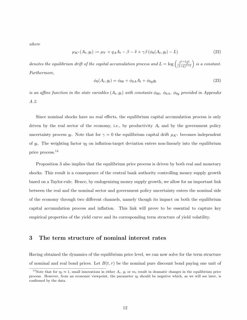
where
µK∗(At, gt) := µY + qAAt − β − δ + γβ (φ0(At, gt)− L) (22)
denotes the equilibrium drift of the capital accumulation process and L = log(
β1+ξξξ
(1+ξ)1+ξ
)is a constant.
Furthermore,
φ0(At, gt) = φ00 + φ0AAt + φ0ggt (23)
is an affine function in the state variables (At, gt) with constants φ00, φ0A, φ0g provided in Appendix
A.2.
Since nominal shocks have no real effects, the equilibrium capital accumulation process is only
driven by the real sector of the economy, i.e., by productivity At and by the government policy
uncertainty process gt. Note that for γ = 0 the equilibrium capital drift µK∗ becomes independent
of gt. The weighting factor η2 on inflation-target deviation enters non-linearly into the equilibrium
price process.14
Proposition 3 also implies that the equilibrium price process is driven by both real and monetary
shocks. This result is a consequence of the central bank authority controlling money supply growth
based on a Taylor-rule. Hence, by endogenizing money supply growth, we allow for an important link
between the real and the nominal sector and government policy uncertainty enters the nominal side
of the economy through two different channels, namely though its impact on both the equilibrium
capital accumulation process and inflation. This link will prove to be essential to capture key
empirical properties of the yield curve and its corresponding term structure of yield volatility.
3 The term structure of nominal interest rates
Having obtained the dynamics of the equilibrium price level, we can now solve for the term structure
of nominal and real bond prices. Let B(t, τ) be the nominal pure discount bond paying one unit of
14Note that for η2 ≈ 1, small innovations in either At, gt or mt result in dramatic changes in the equilibrium priceprocess. However, from an economic viewpoint, the parameter η2 should be negative which, as we will see later, isconfirmed by the data.
12
currency in t+ τ periods. The price of the nominal bond must satisfy the following Euler equation
B(t, τ) = e−βτEt
[UC(C∗t+τ ,M
d∗t+τ )
UC(C∗t ,Md∗t )
p∗tp∗t+τ
]= e−βτEt
[exp− log
(K∗t+τ
)
exp− log (K∗t )p∗tp∗t+τ
], (24)
which states that in equilibrium the investor should be indifferent between consuming one more unit
of currency now or investing one unit of currency in the t+ τ period nominal discount bond.
Proposition 4 (Equilibrium Nominal Term Structure of Interest Rates). Under time-separable
CRRA utility as in Equation (2), the nominal discount bond B(t, τ) with maturity τ is given by
B(t, τ) = exp −b0(τ)− bA(τ)At − bg(τ)gt − bm(τ)mt (25)
where
bA(τ) = CA1− e−κAτ
κA, (26)
−b′g(τ) = Z0g(τ) + Z1g(τ)bg(τ) + Z2gb2g(τ) , (27)
bm(τ) =−Z1m +Hm Cot
(12
(−Hmτ − Tan
(2√Z0mZ2mHm
)))2Z2m
, Hm = 4Z0mZ2m − Z21m, (28)
b0(τ) =
∫ τ
0C0(u)du (29)
and the constant parameters Z0m, Z2i, i ∈ g,m and Z0g(τ), Z1g(τ), C0(τ) are time-to-maturity
functions that only depend on the structural model parameters of the economy and are defined in
Appendix A.3.
The nominal term structure of interest rates in Proposition 4 belongs to the general affine class of
term structure models of discount bond prices introduced by Duffie & Kan (1996). Using Equation
(25), we obtain the time t yield curve Y (t, τ) with maturity τ as
Y (t, τ) := −1
τlog (B(t, τ)) =
b0(τ)
τ+bA(τ)
τAt +
bg(τ)
τgt +
bm(τ)
τmt (30)
The affine yield model in Equation (30) is driven by three factors. As noted, e.g., by Litterman &
Scheinkman (1991), such a three factor structure model of the term structure is able to reproduce
most if not all empirically relevant shapes of the yield curve, such as upward sloping, inverted or
hump shapes. The affine property in the factor loadings implies linearity of the local variance as in
Vasicek (1977), Cox et al. (1985), and others.
13
Analyzing the expressions for the constant and time-varying parameters Z·,·, Z0g(τ), and C0(τ)
given in Appendix A.3, we make the following three observations. First, the target growth rates for
output k and inflation π, the depreciation rate δ, and output µY and money supply growth rate µM
solely affect the intercept of the yield curve but not its slope. In contrast, their weighting factors η1
and η2 affect both the intercept and the slope of the yield curve. Moreover, they do so in a non-linear
way.
Second, the parameter λ has a key impact not only on the level of the term structure but also
on its slope. The parameter λ affects the level of yields, since both CA = CA(λ) and Cg = Cg(λ)
enter the expression for b0(τ) and are functions of λ. This dependence in turn implies that λ also
affects the slope of the term structure through bA(τ) and bg(τ). Furthermore, λ also determines the
long run level of productivity At. To see this, recall that the trend growth rate of the productivity
process At is not only dependent on the long run level of productivity θA but also on the long run
level government policy θg.15 Suppose that θg > 0 and λ < 0, and θA +
λθgκA
< 0, the term bA(τ)τ At,
provided that bA(τ) > 0, will be positive with high probability and therefore will lead to a declining
yield curve for any maturity.
Third, the subjective discount factor β and the degree of transaction service money provides ξ
also impact the slope of the yield curve through the factor loadings bA(τ) and bg(τ) whenever γ 6= 0.
Hence, if the representative agent would have log-utility, β and ξ would only exhibit a level effect.
In the following section we explore the impact of government and monetary policy uncertainty on
the nominal term structure of interest rates in more detail.
3.1 Fitting the model to the data
To fit the model to the term structure data we proceed as follows. We estimate a subset of parameters
using maximum likelihood estimation (MLE) and calibrate the remaining parameters to the nominal
yield and its corresponding volatility curve simultaneously. We estimate the parameters of the policy
uncertainty variables gt and mt using (exact) maximum likelihood estimation.16 Table 1 summarizes
15In particular, we have E[At] = θA +λθgκA
(see Equation (8) in Proposition 1).16Since for the Feller diffusion the transition density is known in closed-form (non-central chi-squared), the transition
density does not need to be approximated via quasi maximum likelihood techniques.
14
the results.
GPU MPU
κg θg σg κm θm σm
Estimate 0.203 0.931 0.326 0.418 0.935 0.285Stand. Error (0.05) (0.104) (0.021) (0.062) (0.043) (0.022)
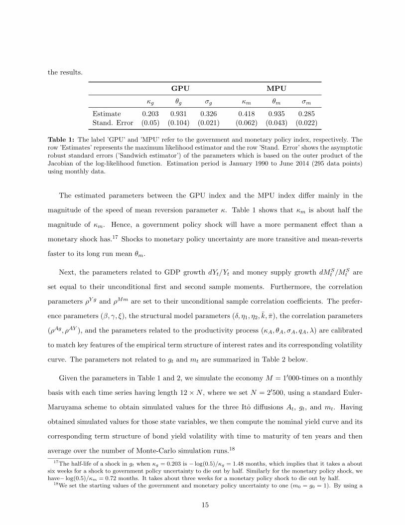
Table 1: The label ’GPU’ and ’MPU’ refer to the government and monetary policy index, respectively. Therow ’Estimates’ represents the maximum likelihood estimator and the row ’Stand. Error’ shows the asymptoticrobust standard errors (’Sandwich estimator’) of the parameters which is based on the outer product of theJacobian of the log-likelihood function. Estimation period is January 1990 to June 2014 (295 data points)using monthly data.
The estimated parameters between the GPU index and the MPU index differ mainly in the
magnitude of the speed of mean reversion parameter κ. Table 1 shows that κm is about half the
magnitude of κm. Hence, a government policy shock will have a more permanent effect than a
monetary shock has.17 Shocks to monetary policy uncertainty are more transitive and mean-reverts
faster to its long run mean θm.
Next, the parameters related to GDP growth dYt/Yt and money supply growth dMSt /M
St are
set equal to their unconditional first and second sample moments. Furthermore, the correlation
parameters ρY g and ρMm are set to their unconditional sample correlation coefficients. The prefer-
ence parameters (β, γ, ξ), the structural model parameters (δ, η1, η2, k, π), the correlation parameters
(ρAg, ρAY ), and the parameters related to the productivity process (κA, θA, σA, qA, λ) are calibrated
to match key features of the empirical term structure of interest rates and its corresponding volatility
curve. The parameters not related to gt and mt are summarized in Table 2 below.
Given the parameters in Table 1 and 2, we simulate the economy M = 1′000-times on a monthly
basis with each time series having length 12×N , where we set N = 2′500, using a standard Euler-
Maruyama scheme to obtain simulated values for the three Ito diffusions At, gt, and mt. Having
obtained simulated values for those state variables, we then compute the nominal yield curve and its
corresponding term structure of bond yield volatility with time to maturity of ten years and then
average over the number of Monte-Carlo simulation runs.18
17The half-life of a shock in gt when κg = 0.203 is − log(0.5)/κg = 1.48 months, which implies that it takes a aboutsix weeks for a shock to government policy uncertainty to die out by half. Similarly for the monetary policy shock, wehave− log(0.5)/κm = 0.72 months. It takes about three weeks for a monetary policy shock to die out by half.
18We set the starting values of the government and monetary policy uncertainty to one (m0 = g0 = 1). By using a
15
Model Parameters
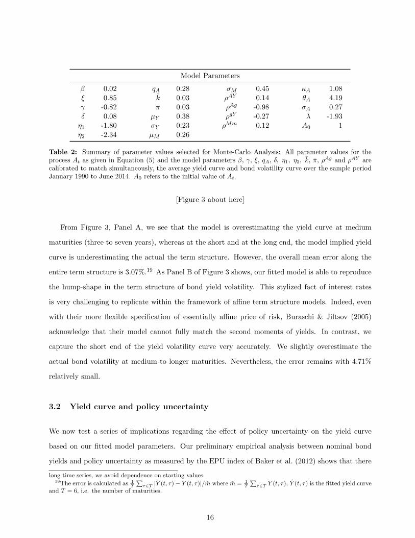
β 0.02 qA 0.28 σM 0.45 κA 1.08ξ 0.85 k 0.03 ρAY 0.14 θA 4.19γ -0.82 π 0.03 ρAg -0.98 σA 0.27δ 0.08 µY 0.38 ρgY -0.27 λ -1.93η1 -1.80 σY 0.23 ρMm 0.12 A0 1η2 -2.34 µM 0.26
Table 2: Summary of parameter values selected for Monte-Carlo Analysis: All parameter values for theprocess At as given in Equation (5) and the model parameters β, γ, ξ, qA, δ, η1, η2, k, π, ρAg and ρAY arecalibrated to match simultaneously, the average yield curve and bond volatility curve over the sample periodJanuary 1990 to June 2014. A0 refers to the initial value of At.
[Figure 3 about here]
From Figure 3, Panel A, we see that the model is overestimating the yield curve at medium
maturities (three to seven years), whereas at the short and at the long end, the model implied yield
curve is underestimating the actual the term structure. However, the overall mean error along the
entire term structure is 3.07%.19 As Panel B of Figure 3 shows, our fitted model is able to reproduce
the hump-shape in the term structure of bond yield volatility. This stylized fact of interest rates
is very challenging to replicate within the framework of affine term structure models. Indeed, even
with their more flexible specification of essentially affine price of risk, Buraschi & Jiltsov (2005)
acknowledge that their model cannot fully match the second moments of yields. In contrast, we
capture the short end of the yield volatility curve very accurately. We slightly overestimate the
actual bond volatility at medium to longer maturities. Nevertheless, the error remains with 4.71%
relatively small.
3.2 Yield curve and policy uncertainty
We now test a series of implications regarding the effect of policy uncertainty on the yield curve
based on our fitted model parameters. Our preliminary empirical analysis between nominal bond
yields and policy uncertainty as measured by the EPU index of Baker et al. (2012) shows that there
long time series, we avoid dependence on starting values.19The error is calculated as 1
T
∑τ∈T |Y (t, τ)− Y (t, τ)|/m where m = 1
T
∑τ∈T Y (t, τ), Y (t, τ) is the fitted yield curve
and T = 6, i.e. the number of maturities.
16

is significant negative correlation between economic policy uncertainty and movements in the yield
curve. Splitting the index into government and monetary policy uncertainty shows that the GPU
index maintains high negative correlation whereas the MPU index seems to have no correlation with
nominal yields at any maturity. Using our affine yield model, we can compute the model-implied
correlation in a straightforward way. More specifically, we can show that a higher level (gt or mt) in
either fiscal or monetary policy uncertainty will lead to a downward shift in yields.
Proposition 5 (Model-implied correlation and impact of policy uncertainty on the yield curve). 1.
Nominal yields are negatively correlated with either fiscal (gt) or monetary (mt) policy uncer-
tainty, i.e.
% [Y (t, τ), gt] ≤ 0, % [Y (t, τ),mt] ≤ 0, ∀τ ≥ 0
and the effect is stronger for fiscal as opposed to monetary policy uncertainty, in other words
|% [Y (t, τ), gt] | > |% [Y (t, τ),mt] |
2. Nominal yields yields are decreasing in both fiscal (gt) and monetary (mt) policy uncertainty
∂Y (t, τ)
∂gt=bg(τ)
τ< 0,
∂Y (t, τ)
∂mt=bm(τ)
τ< 0, ∀τ ≥ 0. (31)
and this effect is again stronger for fiscal as opposed to monetary policy uncertainty, i.e.,∣∣∣∣bg(τ)
τ
∣∣∣∣ > ∣∣∣∣bm(τ)
τ
∣∣∣∣ , ∀τ ≥ 0. (32)
The results in Proposition 5 above are in line with the empirical observations. The reason why the
model implied correlation is negative for any maturity can be directly deduced from the covariance
between Y (t, τ) and gt which is,
C[Y (t, τ), gt] =bA(τ)
τ
θgσg(2κgλρ
AgσA + λσg)
2κg(κA + κg)+bg(τ)
τ
θgσ2g
2κg. (33)
Given the fitted parameters in Table 1 and 2, the factor loading bA(τ) is always positive whereas
bg(τ) is negative, which implies that the first and second term in Equation (33) will be negative.
In this setting, we obtain a model-implied average (along maturity τ) correlation of -0.2934 which
is comparable to the empirical sample correlation between nominal yields and the GPU (-0.40).
Likewise, since bm(τ) ≤ 0 we obtain C(Y (t, τ),mt) = θmσ2m
2κm
bm(τ)τ ≤ 0, ∀τ ≥ 0. Comparing this model
17

correlation coefficient of -0.021 to its empirical counterpart (-0.011), we see that the model is able
to match both sample correlation coefficients.
3.3 Equilibrium nominal short rate and bond excess returns
We now discuss how the short end of the term structure of interest rates and the bond risk premium
are affected by government and monetary policy uncertainty.
Proposition 6 (Equilibrium nominal short rate and bond risk premium). With time-separable
CRRA utility, we have the following first order asymptotic results:
1. The nominal short rate Rt is given by
Rt =(µY − β − δ − k)η1 + β + µM − η2(µY + π − δ)
1− η2+ γ
β(η1 − η2)(L− φ00)
1− η2−
σ2M
(η2 − 1)2mt
− (qA + γβφ0A)
(η1 − η2
η2 − 1
)At −
((η1 − η2)2σ2
Y
(η2 − 1)2+ γ
βφ0g(η1 − η2)
η2 − 1
)gt (34)
2. The nominal price of fiscal risk λN,gt as well as the market price of monetary risk λN,mt are
λN,gt =η2 − η1
η2 − 1σY√gt, λN,mt =
σMη2 − 1
√mt. (35)
3. The bond risk premia RP (t, τ) per unit of time is given by
RP (t, τ) :=1
dtEt[dB(t, τ)
B(t, τ)−Rtdt
]= λN,Yt
[bA(τ)ρAY σA + bg(τ)ρgY σg
]√gt + λN,Mt bm(τ)ρMmσm
√mt (36)
= ΛN,gt + ΛN,mt (37)
where ΛN,gt = λN,Yt
[bA(τ)ρAY σA + bg(τ)ρgY σg
]√gt and ΛN,mt = λN,Mt bm(τ)ρMmσm
√mt are
the factor loadings of government and monetary policy uncertainty, respectively.
The nominal short rate and the nominal market price of risk are all influenced by both the real
and nominal sector of the economy, which is a direct consequence of the Taylor rule in Assumption
4. In the special case when money supply is entirely decoupled from the real sector (η1 = η2 = 0),
the nominal short rate reduces to Rt = µM + β − σ2Mmt and λN,Yt = 0 so that the real side does
18

not affect the nominal short rate and output risk is no longer a nominal risk factor. We get the
same result when η1 = η2 = η, i.e., when the central bank reacts to deviations from its nominal
and real targets equally. Then, the nominal short rate is also an affine function of mt and the risk
premium does not depend on gt. In both cases, the nominal short rate becomes independent of the
risk aversion parameter γ.
In the general case, Rt depends on the money supply control variables η1 and η2 in a non-linear
way. This suggests that relatively small fluctuations in either productivity At, monetary or govern-
ment policy uncertainty may lead to drastic movements in the nominal short rate. Furthermore, risk
aversion affects Rt through different channels. First, it affects its level through the second term in
Equation (34). If risk aversion increases, i.e., if γ decreases, the short rate becomes smaller since
β(η1−η2)(L−φ00)η2−1 > 0. Secondly, the risk aversion coefficient γ loads on both real sector variables At
and gt. Therefore, risk aversion also impacts the slope and curvature of the term structure. To
what extent risk aversion changes slope and curvature depends on the magnitude of the estimated
parameter values.
When η1 6= 0 and η2 6= 0, the nominal price of risk decomposes into two state-dependent market
prices of risks λN,Yt and λN,Mt , which are driven by government and monetary policy risk, respec-
tively.20 Furthermore, the sign of those market prices of risk is determined by η1 and η2, the
parameters controlling the intensity of adjustments to the long run real output growth target k and
inflation target π and therefore can become negative depending on the values of η1 and η2.
[Figure 4 about here]
For the bond risk premium in Equation (37), we plot in Figure 4, Panel A, the loadings of the
government policy uncertainty factor gt and the monetary policy uncertainty factor mt. Under our
estimated parameters, both government and monetary policy uncertainty load positively on the risk
premium. Monetary policy uncertainty has a larger impact at the short end of the curve, but flattens
out at longer maturities and eventually becomes dominated by government policy uncertainty. Hence,
20The results in Proposition 6 reveal that equilibrium relations such as the expected bond excess premium andinterest rate volatility as well as the forward term premium, i.e., violation of the expectation hypothesis, will be drivenby government and monetary policy uncertainty whenever η1 6= 0 and η2 6= 0.
19

our model predicts that the dominant factor at the short end is monetary policy uncertainty, while
the dominant role at the long end of the bond risk premia curve is played by the government policy
uncertainty factor.
3.4 Bond yield volatility
Many empirical studies find that long run bond yields exhibit higher volatility than implied by
the expectation hypothesis. Already Shiller (1979) shows that long term bond yields exhibit excess
volatility relative to their model-implied values. From Piazzesi & Schneider (2006) we know that their
representative agent-based model explains a smaller fraction of observed volatility of the long-end
yields than of the short-end yields. Xiong & Yan (2010) argue that excess bond volatility might be due
to differences in beliefs about the long run level of inflation. They show that a higher belief dispersion
leads to volatility amplification which allows them to account not only for the empirically observed
high bond yield volatility, but also for the hump-shape of the term structure of bond volatility.21 To
explore the key determinants that allow to reproduce the hump-shape in bond volatility, we need to
derive the model-implied unconditional variance of nominal yields. It turns out that the variance is
a linear combination of the variances of monetary and government policy uncertainty, the variance
of productivity, and the covariance of productivity and government policy uncertainty.
Corollary 1 (Term Structure of Nominal Bond Yield Variance). Let Y (t, τ) denote the current time
t yield with maturity τ . Then the unconditional term structure of bond yield variance is given by
V[Y (t, τ)] =b2A(τ)
τ2V[At] +
b2g(τ)
τ2V[gt] +
b2m(τ)
τ2V[mt] + 2
bA(τ)bg(τ)
τ2C[At, gt] (38)
where V[mt] = θmσ2m
2κmand the expressions for V[At], C[At, gt], and V[gt] are given in Proposition 1.
To explore the key determinants in generating the hump-shape in bond yield variance, Figure 4
plots the different components contributing to the bond yield variance in Equation (38).
[Figure 4 about here]
21Closely related to the ’excess volatility puzzle’ phenomenon are also the findings of Gurkaynak et al. (2005b). Theydocument that bond yields exhibit excess sensitivity to macroeconomic announcements.
20

The contribution of both the factor loadings bg(τ) and the cross term bA(τ)bg(τ) are hump shaped,
which causes the term structure of yield variance to exhibit a similar pattern. The government policy
factor gt exhibits a hump shape that peaks around the two year maturity. The covariance term
C(At, gt) is also contributing significantly to the hump. Its magnitude is determined by two factors,
by the correlation between government policy uncertainty and productivity (ρAg < 0) and by the
impact of government policy uncertainty on productivity (λ < 0). The impact of the production
variance V[At] as well as of monetary policy uncertainty is monotonically decreasing in τ . The latter
factor has only little impact. From Corollary 1 and Figure 4 we can deduce the following:
Proposition 7 (Policy Uncertainty and the term structure of bond yield volatility).
Government gt and monetary mt policy uncertainty raise the level of bond yield volatility.
However, the effect is much stronger for fiscal as opposed to monetary policy uncertainty, i.e.
b2g(τ)
τ2V[gt] >
b2g(τ)
τ2V[mt] (39)
The function F g(τ) =b2g(τ)
τ2V[gt] is hump-shaped across maturities. This implies that the effect
of government policy uncertainty is highest for about 2 years maturity according to Figure 4.
The first result in Proposition 7 is straight-forward. Since clearlyb2g(τ)
τ2V[gt] > 0,
(b2m(τ)τ2
V[mt] > 0)
and C(At, gt) > 0 adding the government (monetary) policy uncertainty factor raises the level of
volatility. The second statement above is far less obvious to see, as it crucially depends on the
parameter specifications of the model. Therefore, in Panels A through F of Figure 5, we explore in
more detail the parameters responsible for generating the hump shape.
[Figure 5 about here]
As Panel A illustrates, the term structure of bond yield volatility exhibits a fundamentally dif-
ferent shape whenever λ is negative or when λ is set to zero, in which case government policy
uncertainty does not affect the drift of productivity. Not only is the level of the term structure
significantly higher whenever λ < 0 than compared to the case when λ = 0 but also, bond yield
volatility becomes hump-shaped in time to maturity. Panels B and C show that the speed of mean
21

reversion level κg and volatility σg have a similar effect on bond volatility. A more persistent and a
highly volatile uncertainty process generate not only to an upward shift of the bond volatility term
structure, but also a hump shape.22 Similar to Panel B, we observe in Panel D that a more perma-
nent shock in productivity (decrease in κA) also accentuates the hump shape. In contrast, increasing
production volatility σA shifts the volatility term structure upward such that it eventually becomes
monotonically decreasing (Panel E). This follows because the factorb2A(τ)
τ2V(At) increases proportion-
ally in σ2A and since
b2A(τ)
τ2is monotonically decreasing. Finally, Panel F shows that bond volatility
is highly sensitive to changes in either η1 or η2. When the central bank becomes less responsive
to deviations of the long term real target k, the level of bond volatility decreases substantially. In
contrast, if the central bank becomes less responsive to deviations of the long term nominal target
π, bond volatility increases significantly.23
4 Empirical analysis
Our theoretical model gives rise to several theoretical predictions. In the subsequent empirical
analysis, we examine the following four testable hypotheses.
Hypothesis 1 (H1): Our first prediction can be deduced directly from Proposition 5, which
implies that nominal yields fall when either government or monetary policy uncertainty increases
and vice versa. From Proposition 5, this effect is mainly driven by government policy uncertainty
(see Equation (31)).
Hypothesis 2 (H2): Higher (lower) fiscal or monetary policy uncertainty increases (decreases)
nominal yield volatility (see Equation (39) in Proposition 7). This effect is again mainly driven by
government policy uncertainty.
22The long run mean of government policy uncertainty θg increases yield dispersion proportionally, since ∂V(Y (t,τ)∂θg
> 0.
Hence, the long term mean does not contribute to a hump shape.23Without providing the corresponding plots, we remark that whenever both η1 and η2 are both reduced, there will
be a parallel downward shift in the level of bond yield volatility. Furthermore, the impact of risk aversion on the termstructure of bond volatilities is less pronounced and leads to an almost parallel downward shift of the term structure.
22
Hypothesis 3 (H3): From the second result in Proposition 7, the hump shape of the term structure
of bond yield volatility is mainly driven by government policy uncertainty and not by monetary policy
uncertainty.
Hypothesis 4 (H4): From Equation (37), bond risk premia are affected by both monetary and
government policy uncertainty.
To investigate the joint effect of government and monetary policy uncertainty on the yield curve,
its term structure of volatility, and on risk premia, we use as a proxy for both types of policy
uncertainties, the economic policy uncertainty (EPU) index developed by Baker et al. (2012). Thus,
in our model this index would be approximately equivalent to setting EPUt ≈ gt + mt. In what
follows, we will empirically test the above hypotheses by regressing nominal yields and yield volatility
on the EPU index and our time series of government and monetary policy as well as a set of control
variables.
4.1 Data
We obtain monthly Treasury Bill yields with maturity one, two, three, five, seven, and ten years from
the Federal Reserve Board ranging from January 1990 until July 2014, from which we bootstrap the
zero-coupon yield curve treating the treasury yields as par yields. From Datastream, we collect
monthly data on a total of 2 macro variables, which we aggregate into a real business cycle activity
factor and an inflation factor.24 As a measure for real activity we use industrial production (IP). As
an inflation factor, we use the consumer price index (CPI). We then compute monthly log-growth
rates over one year for each of the macro control variables.
As an alternative to the EPU, we proxy for (policy) uncertainty using the VIX index. As a
measure for economic condition we include the Chicago Fed National Activity Index (CFNAI), which
we obtain from the FRED database (St. Louis Fed).25 We also use treasury bond implied volatility
24Similar control variables have also been used by Ang & Piazzesi (2003), Evans & Marshall (2007), Ludvigson &Ng (2009) or Joslin, Priebisch & Singleton (2014) in their study of the economic determinants of the term structure ofnominal interest rates.
25The reason why we include the CFNAI regressor is to test whether either monetary or government policy uncertaintyhas predictive power after controlling for the state the economy is in. This is because it is reasonable to assume thatuncertainty about the government’s future policy choice is in general larger in weaker economic conditions.
23
(TIV) based on weighted average of one-month options on treasury bonds with maturity of two, five,
ten, and 30 years as a proxy for bond market volatility.
In addition we collect two time series, which we refer to as Financial Variables’ (FV). They
include the monthly log growth rate of the S&P composite dividend yield index (DY), which has
been shown to have forecasting power by Fama & French (1989), and the term spread measured as
the ten-year yield less the federal funds rate (TS).
4.2 Construction of government and monetary policy uncertainty index
The economic policy uncertainty (EPU) index developed by Baker et al. (2012) has been recently used
by a number of studies.26 The EPU index is constructed from three main components, namely a news
impact part which is based on news paper discussing economic policy uncertainty, a component that
summarizes reports by the Congressional Budget Office (CBO) that compile lists of temporary federal
tax code provisions, and a third component called ‘economic forecaster disagreement’, which draws
on the Federal Reserve Bank of Philadelphia’s Survey of Professional Forecasters and summarizes
data on consumer price forecast dispersion and predictions for purchases of goods and services by
state, local and federal government.27
For our setting, we need to decompose the EPU index into uncertainty related to government
and monetary policy. To disentangle the two types of uncertainties, we use the ‘categorical EPU
data’, which contains time-series on uncertainty related to government and monetary policy as well
as further categorical variables.28 For our measure of government policy uncertainty, we extract the
time-series ‘fiscal policy’, ‘taxes’, and ‘government spending’. Furthermore, we argue that disagree-
ment about temporary federal tax code provisions and forecast variation in local state and federal
purchases of goods and services are sources of government policy uncertainty, whereas disagreement
26For instance, Pastor & Veronesi (2013) show that government policy uncertainty carries a risk premium, and thatstocks are more volatile and more correlated in times of high uncertainty. Brogaard & Detzel (2012) use the sameindex and find that economic policy uncertainty forecast future market excess returns. Similarly, Gulen & Ion (2012)show that policy-related uncertainty is negatively correlated with firm and industry level investment. When policyuncertainty increases firm’s tend to reduce their investment.
27As Kelly et al. (2013) argue, it is difficult isolate exogenous variation in political uncertainty as it likely depends onvarious factors such as overall macro uncertainty. Therefore, the EPU index may not only capture government relateduncertainty, but can be interpreted as a broader measure of uncertainty about economic fundamentals.
28This data is also available from http://www.policyuncertainty.com/.
24
about future inflation (CPI disagreement) can be related to monetary uncertainty.
Therefore, in order to construct our index of ‘government policy uncertainty’ labeled as ‘GPU’ we
include the time series ‘fiscal policy’, ’Taxes’, ’Government’, ‘FedStateLocal Ex disagreement’ and
‘Tax expiration’. We place half of the weight to the time series ‘fiscal policy’ and the other half is
equally distributed among the time series ’Taxes’, ’Government’, ’FedStateLocal Ex disagreement’
and ’Tax expiration’.29 Our measure of ‘monetary policy’ uncertainty, which we abbreviate by
‘MPU’, consists of the time series ‘monetary policy uncertainty’ and ‘CPI disagreement’ of which
each obtain weight 1/2.
4.3 Policy uncertainty and the yield curve
To investigate the relationship between the yield curve and the EPU index, we make the following
regression,
Y (t, τ) = β0 + β1PUt + εt, PUt ∈ EPUt, GPUt,MPUt, (40)
where PUt denotes either the EPU, GPU, or MPU index at time t, and εt is the regression error
term.30
According to hypothesis H1, we expect the coefficient in Equation (40) to be negative for all
the three uncertainty indexes. Additionally, we run the same regression as in Equation (40) above,
just replacing the PUt index with the VIX index. Since the VIX index is a generally accepted
measure of overall economic uncertainty and positively correlated with the EPU index,31 we expect
the regression coefficient to be negative as well. We also regress Y (t, τ) on both the VIX and the
EPU index, and on the VIX together with the GPU and MPU indices. By doing so, we can identify
those variables that exhibit greater predictive power.
In Table 3 we summarize the results for the EPU index.32 The first row labeled ‘EPU’ shows that
29We divided the time series ‘Tax expiration’ by a factor of ten, because its impact would otherwise pull the index upsubstantially at the end of the time series. Furthermore, as tax laws are only altered infrequently, the ‘Tax expiration’remains constant over several months up to two years. Its unscaled inclusion would lead to an underestimation inpolicy uncertainty variation.
30To address potential concerns about robustness of our results, we compute following Newey & West (1994) standarderrors with five lags to account for heteroskedasticity and autocorrelation (HAC) in residuals.
31For our sample, the correlation coefficient between VIX and EPU is 0.45.32For all the regressions tables that follow the intercept estimate β0 and corresponding HAC errors are not displayed.
25
τ 1Y 2Y 3Y 5Y 7Y 10Y
EPU EPU -3.70*** -3.68*** -3.51*** -3.02*** -2.61*** -2.16***tEPU (-7.08) (-6.95) (-6.61) (-5.67) (-4.95) (-4.19)R2adj 0.29 0.29 0.28 0.24 0.21 0.17
VIX VIX -0.04 -0.05* -0.05* -0.05* -0.04* -0.04*tV IX (-1.50) (-1.67) (-1.76) (-1.86) (-1.78) (-1.91)R2adj 0.02 0.02 0.02 0.02 0.02 0.03
EPU & VIX EPU -4.07*** -4.00*** -3.78*** -3.19*** -2.75*** -2.13***tEPU (-8.26) (-7.77) (-7.17) (-5.76) (-4.80) (-3.75)VIX 0.04 0.03 0.03 0.02 0.01 0.01tV IX (1.62) (1.37) (1.17) (0.75) (0.58) (0.15)R2adj 0.30 0.30 0.29 0.24 0.21 0.16
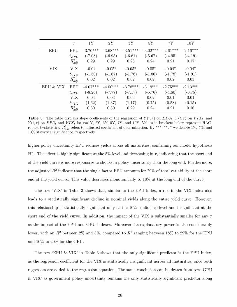
Table 3: The table displays slope coefficients of the regression of Y (t, τ) on EPUt, Y (t, τ) on V IXt, andY (t, τ) on EPUt and V IXt for τ=1Y, 2Y, 3Y, 5Y, 7Y, and 10Y. Values in brackets below represent HAC-robust t−statistics. R2
adj refers to adjusted coefficient of determination. By ***, **, * we denote 1%, 5%, and10% statistical significance, respectively.
higher policy uncertainty EPU reduces yields across all maturities, confirming our model hypothesis
H1. The effect is highly significant at the 5% level and decreasing in τ , indicating that the short end
of the yield curve is more responsive to shocks in policy uncertainty than the long end. Furthermore,
the adjusted R2 indicate that the single factor EPU accounts for 29% of total variability at the short
end of the yield curve. This value decreases monotonically to 18% at the long end of the curve.
The row ‘VIX’ in Table 3 shows that, similar to the EPU index, a rise in the VIX index also
leads to a statistically significant decline in nominal yields along the entire yield curve. However,
this relationship is statistically significant only at the 10% confidence level and insignificant at the
short end of the yield curve. In addition, the impact of the VIX is substantially smaller for any τ
as the impact of the EPU and GPU indexes. Moreover, its explanatory power is also considerably
lower, with an R2 between 2% and 3%, compared to R2 ranging between 18% to 29% for the EPU
and 10% to 20% for the GPU.
The row ‘EPU & VIX’ in Table 3 shows that the only significant predictor is the EPU index,
as the regression coefficient for the VIX is statistically insignificant across all maturities, once both
regressors are added to the regression equation. The same conclusion can be drawn from row ‘GPU
& VIX’ as government policy uncertainty remains the only statistically significant predictor along
26

the entire term structure. Lastly, row ‘MPU & VIX’ shows that the MPU index has no predictive
power for any τ .
To check for the robustness of our results, we add different controls to the regression equation.
We add the economic condition (EC) controls ‘CFNAI’ and ‘VIX’. Furthermore, we also include the
financial variables (FV) factor and macro controls (MC) as discussed in Section 4.1.
τ 1Y 2Y 3Y 5Y 7Y 10Y
EC EPU -4.14*** -4.05*** -3.83*** -3.24*** -2.78*** -2.17***tEPU (-9.51) (-8.79) (-7.95) (-6.15) (-5.10) (-4.03)R2adj 0.30 0.30 0.28 0.24 0.21 0.16
EC+FV EPU -2.56*** -2.82*** -2.87*** -2.72*** -2.48*** -2.09***tEPU (-4.07) (-4.27) (-4.23) (-3.91) (-3.62) (-3.22)R2adj 0.47 0.40 0.35 0.26 0.22 0.17
EC+FV+MC EPU -2.75** -3.02** -3.07** -2.91** -2.66** -2.28**tEPU (-5.60) (-5.81) (-5.75) (-5.47) (-5.14) (-4.73)R2adj 0.62 0.56 0.52 0.47 0.44 0.42
Table 4: The table reports slope coefficients of the regression, Y (t, τ) on EPUt and EC controls (EC), Y (t, τ)on EPUt and EC, FV variables (EC+FV), Y (t, τ) on EPUt and Y (t, τ) on EPUt, and EC, FV, MC controls(Full Reg.) for τ = 1Y, 2Y, 3Y, 5Y, 7Y and 10Y. Values in brackets below represent HAC-robust t−statistics.R2adj refers to adjusted coefficient of determination. By ***, **, * we denote 1%, 5%, and 10% statistical
significance, respectively.
Table 4 shows that the EPU regression coefficient remains significant for any maturity and across
all regressions. However, compared to Table 3, its impact is considerably reduced (primarily at the
short end), especially when we include the financial variables (FV). The reason for this decline is
because those regressors exhibit strong positive correlation with the EPU index. Not surprisingly,
their estimated impact on contemporaneous yield changes is also negative. Their average is -4.62
(DY), and -0.16 (TS). Whereas the R2adj essentially stays the same after adding the CFNAI control
(row ’EC’), it increases considerably, although mainly at the short-end of the yield curve, after
adding the financial factors (see row ‘EC+FV’). Lastly, as the row labeled ‘EC,FV+MC’ shows, that
whereas adding macro controls to the regression equation does not impact the statistical significance
and magnitude of the EPU index, it considerably increases the amount of explained variation as the
R2adj increases substationally across every maturity.33
33This increase in R2adj is predominantly driven by inflation as it has a statistically significant, very large and positive
27
[Figure 6 about here]
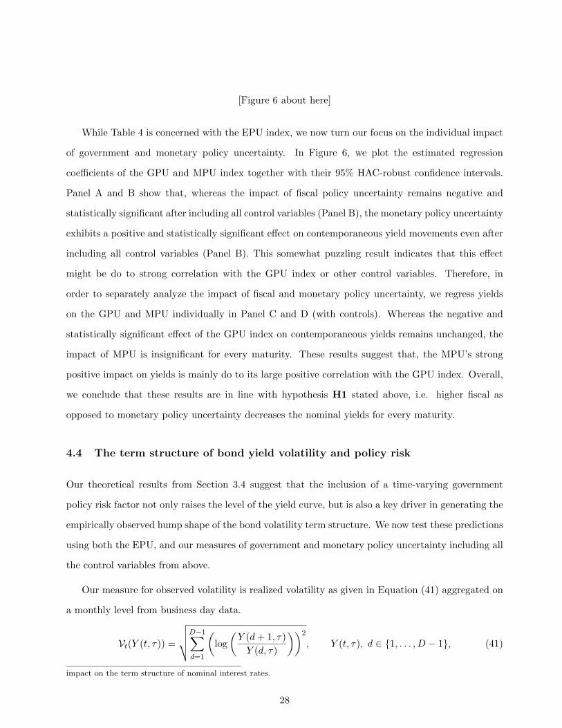
While Table 4 is concerned with the EPU index, we now turn our focus on the individual impact
of government and monetary policy uncertainty. In Figure 6, we plot the estimated regression
coefficients of the GPU and MPU index together with their 95% HAC-robust confidence intervals.
Panel A and B show that, whereas the impact of fiscal policy uncertainty remains negative and
statistically significant after including all control variables (Panel B), the monetary policy uncertainty
exhibits a positive and statistically significant effect on contemporaneous yield movements even after
including all control variables (Panel B). This somewhat puzzling result indicates that this effect
might be do to strong correlation with the GPU index or other control variables. Therefore, in
order to separately analyze the impact of fiscal and monetary policy uncertainty, we regress yields
on the GPU and MPU individually in Panel C and D (with controls). Whereas the negative and
statistically significant effect of the GPU index on contemporaneous yields remains unchanged, the
impact of MPU is insignificant for every maturity. These results suggest that, the MPU’s strong
positive impact on yields is mainly do to its large positive correlation with the GPU index. Overall,
we conclude that these results are in line with hypothesis H1 stated above, i.e. higher fiscal as
opposed to monetary policy uncertainty decreases the nominal yields for every maturity.
4.4 The term structure of bond yield volatility and policy risk
Our theoretical results from Section 3.4 suggest that the inclusion of a time-varying government
policy risk factor not only raises the level of the yield curve, but is also a key driver in generating the
empirically observed hump shape of the bond volatility term structure. We now test these predictions
using both the EPU, and our measures of government and monetary policy uncertainty including all
the control variables from above.
Our measure for observed volatility is realized volatility as given in Equation (41) aggregated on
a monthly level from business day data.
Vt(Y (t, τ)) =
√√√√D−1∑d=1
(log
(Y (d+ 1, τ)
Y (d, τ)
))2
, Y (t, τ), d ∈ 1, . . . , D − 1, (41)
impact on the term structure of nominal interest rates.
28
where D denotes the number of daily observations (about 20 business days per month) and τ=1Y, 2Y,
3Y, 5Y, 7Y and 10Y to construct a time series of monthly realized bond yield volatility. In addition
to our control variables from the previous sections, we also include treasury implied volatility (TIV)
to proxy for fixed-income implied volatility.34
Vt[Y (t, τ)] = β0 + β1PUt + contt + εt, (42)
where PUt denotes either the EPU, GPU, or MPU index at time t, contt summarizes all the control
variables and εt is the regression error term. From our hypothesis H2, we expect the sign of the
regression coefficient in (42) of the EPU and the GPU index to be positive for all maturities.35
Furthermore, from hypothesis H3 we expect that economic or government policy uncertainty have a
hump-shaped effect on the term structure of bond yield volatility. Thus, we should observe that the
estimated regression coefficients peaks around the two year maturity as the realized bond volatility
curve in Figure 3 does.
τ 1 2 3 5 7 10
Simple EPU 0.192*** 0.194*** 0.166*** 0.121*** 0.091*** 0.063***tEPU (7.18) (9.72) (8.88) (8.86) (7.66) (7.01)R2adj 0.37 0.43 0.44 0.43 0.40 0.37
EC EPU 0.192*** 0.188*** 0.156*** 0.111*** 0.079*** 0.051***tEPU (6.39) (9.37) (8.73) (8.60) (7.46) (6.67)R2adj 0.39 0.44 0.45 0.45 0.43 0.43
EC +FV & TIV EPU 0.135*** 0.135*** 0.118*** 0.087*** 0.064*** 0.042***tEPU (4.08) (5.41) (4.99) (4.91) (4.18) (3.70)R2adj 0.44 0.50 0.50 0.48 0.45 0.44
Full Regression EPU 0.146*** 0.145*** 0.125*** 0.095*** 0.071*** 0.04***tEPU (4.27) (6.24) (5.76) (6.62) (5.90) (5.29)R2adj 0.47 0.56 0.57 0.57 0.57 0.56
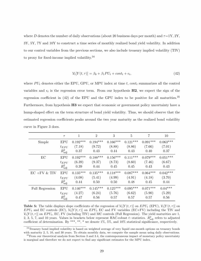
Table 5: The table displays slope coefficients of the regression of Vt[Y (t, τ)] on EPUt (EPU), Vt[Y (t, τ)] onEPUt and EC controls (EC), Vt[Y (t, τ)] on EPUt EC and FV variables (EC+FV) including the TIV andVt[Y (t, τ)] on EPUt, EC, FV (including TIV) and MC controls (Full Regression). The yield maturities are 1,2, 3, 5, 7, and 10 years. Values in brackets below represent HAC-robust t−statistics. R2
adj refers to adjustedcoefficient of determination. By ***, **, * we denote 1%, 5%, and 10% statistical significance, respectively.
34Treasury bond implied volatility is based on weighted average of very liquid one-month options on treasury bondswith maturity 2, 5, 10, and 30 years. To obtain monthly data, we compute the sample mean using daily observations.
35From our theoretical analysis from Section 3 and 3.4, the contemporaneous impact of monetary policy uncertaintyis marginal and therefore we do not expect to find any significant estimates for the MPU index.
29
We report the results of the regression in Equation (42) in Table 5. We find our hypothesis H2
concerning the EPU confirmed. Higher economic policy uncertainty increases bond volatility for any
maturity. Once we include the financial control variables, the impact of the EPU index is reduced
for any maturity and the explanatory power increases from an average R2adj = 0.40 to R2
adj = 0.47.
This observation suggests, similar to the results in Table 4, that financial factors are also important
predictors of bond variance. Analyzing in more detail, we see from row ’Full Regression’ that there
is only a moderate increase in predictive power once we also include our macro controls.
Concerning hypothesis H3, although the impact of economic policy is highly statistically signif-
icant, it gradually declines along the entire term structure. Hence, the EPU index is not able to
generate a hump in the volatility term structure. Therefore, if we would use the EPU as our proxy
for government uncertainty, this result in conflict with our hypothesis H3. However, since in the
EPU index government and monetary uncertainty factors are intermingled, we need to analyze the
impact of the government and monetary policy uncertainty index separately.
[Figure 7 about here]
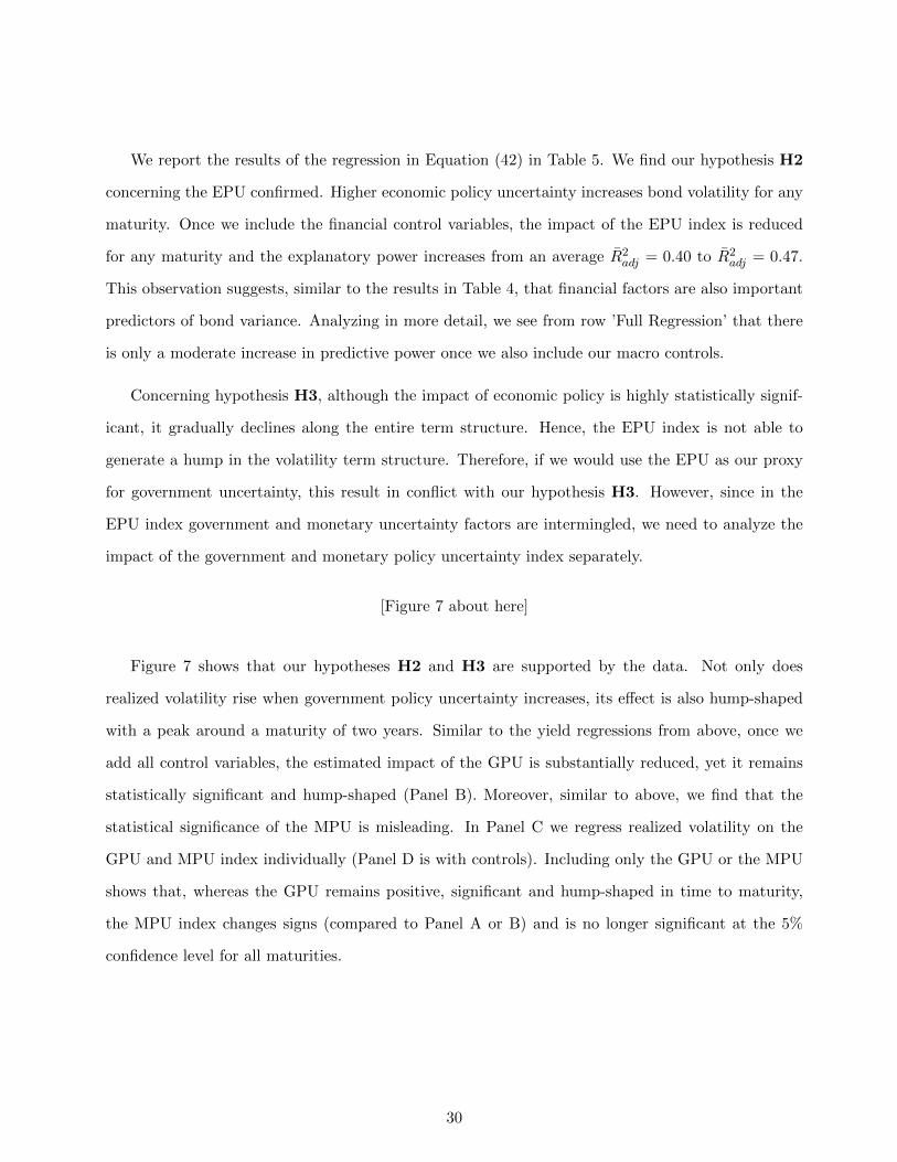
Figure 7 shows that our hypotheses H2 and H3 are supported by the data. Not only does
realized volatility rise when government policy uncertainty increases, its effect is also hump-shaped
with a peak around a maturity of two years. Similar to the yield regressions from above, once we
add all control variables, the estimated impact of the GPU is substantially reduced, yet it remains
statistically significant and hump-shaped (Panel B). Moreover, similar to above, we find that the
statistical significance of the MPU is misleading. In Panel C we regress realized volatility on the
GPU and MPU index individually (Panel D is with controls). Including only the GPU or the MPU
shows that, whereas the GPU remains positive, significant and hump-shaped in time to maturity,
the MPU index changes signs (compared to Panel A or B) and is no longer significant at the 5%
confidence level for all maturities.
30
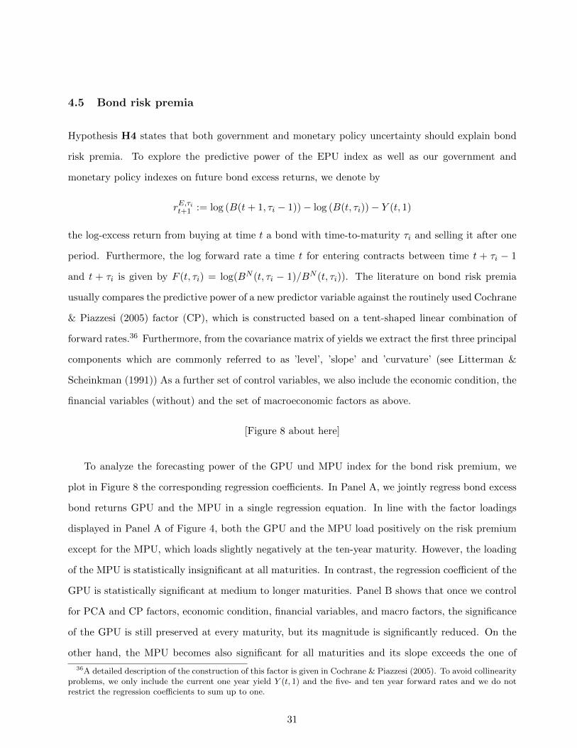
4.5 Bond risk premia
Hypothesis H4 states that both government and monetary policy uncertainty should explain bond
risk premia. To explore the predictive power of the EPU index as well as our government and
monetary policy indexes on future bond excess returns, we denote by
rE,τit+1 := log (B(t+ 1, τi − 1))− log (B(t, τi))− Y (t, 1)
the log-excess return from buying at time t a bond with time-to-maturity τi and selling it after one
period. Furthermore, the log forward rate a time t for entering contracts between time t + τi − 1
and t + τi is given by F (t, τi) = log(BN (t, τi − 1)/BN (t, τi)). The literature on bond risk premia
usually compares the predictive power of a new predictor variable against the routinely used Cochrane
& Piazzesi (2005) factor (CP), which is constructed based on a tent-shaped linear combination of
forward rates.36 Furthermore, from the covariance matrix of yields we extract the first three principal
components which are commonly referred to as ’level’, ’slope’ and ’curvature’ (see Litterman &
Scheinkman (1991)) As a further set of control variables, we also include the economic condition, the
financial variables (without) and the set of macroeconomic factors as above.
[Figure 8 about here]
To analyze the forecasting power of the GPU und MPU index for the bond risk premium, we
plot in Figure 8 the corresponding regression coefficients. In Panel A, we jointly regress bond excess
bond returns GPU and the MPU in a single regression equation. In line with the factor loadings
displayed in Panel A of Figure 4, both the GPU and the MPU load positively on the risk premium
except for the MPU, which loads slightly negatively at the ten-year maturity. However, the loading
of the MPU is statistically insignificant at all maturities. In contrast, the regression coefficient of the
GPU is statistically significant at medium to longer maturities. Panel B shows that once we control
for PCA and CP factors, economic condition, financial variables, and macro factors, the significance
of the GPU is still preserved at every maturity, but its magnitude is significantly reduced. On the
other hand, the MPU becomes also significant for all maturities and its slope exceeds the one of
36A detailed description of the construction of this factor is given in Cochrane & Piazzesi (2005). To avoid collinearityproblems, we only include the current one year yield Y (t, 1) and the five- and ten year forward rates and we do notrestrict the regression coefficients to sum up to one.
31
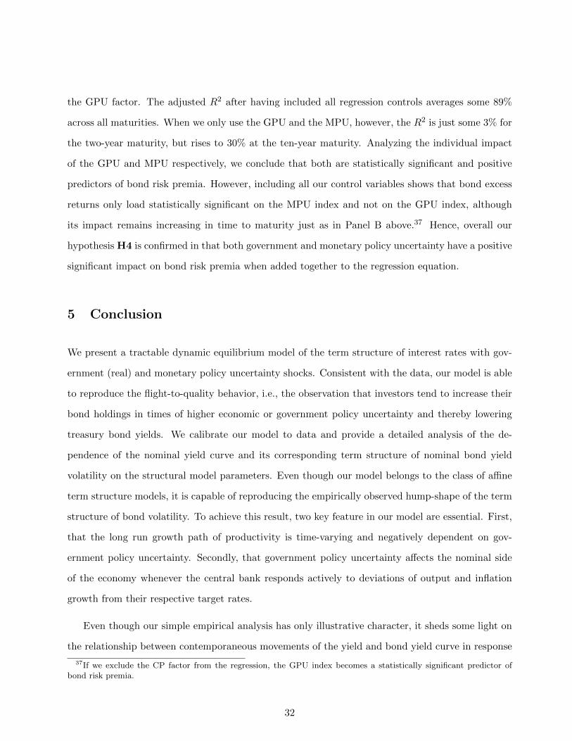
the GPU factor. The adjusted R2 after having included all regression controls averages some 89%
across all maturities. When we only use the GPU and the MPU, however, the R2 is just some 3% for
the two-year maturity, but rises to 30% at the ten-year maturity. Analyzing the individual impact
of the GPU and MPU respectively, we conclude that both are statistically significant and positive
predictors of bond risk premia. However, including all our control variables shows that bond excess
returns only load statistically significant on the MPU index and not on the GPU index, although
its impact remains increasing in time to maturity just as in Panel B above.37 Hence, overall our
hypothesis H4 is confirmed in that both government and monetary policy uncertainty have a positive
significant impact on bond risk premia when added together to the regression equation.
5 Conclusion
We present a tractable dynamic equilibrium model of the term structure of interest rates with gov-
ernment (real) and monetary policy uncertainty shocks. Consistent with the data, our model is able
to reproduce the flight-to-quality behavior, i.e., the observation that investors tend to increase their
bond holdings in times of higher economic or government policy uncertainty and thereby lowering
treasury bond yields. We calibrate our model to data and provide a detailed analysis of the de-
pendence of the nominal yield curve and its corresponding term structure of nominal bond yield
volatility on the structural model parameters. Even though our model belongs to the class of affine
term structure models, it is capable of reproducing the empirically observed hump-shape of the term
structure of bond volatility. To achieve this result, two key feature in our model are essential. First,
that the long run growth path of productivity is time-varying and negatively dependent on gov-
ernment policy uncertainty. Secondly, that government policy uncertainty affects the nominal side
of the economy whenever the central bank responds actively to deviations of output and inflation
growth from their respective target rates.
Even though our simple empirical analysis has only illustrative character, it sheds some light on
the relationship between contemporaneous movements of the yield and bond yield curve in response
37If we exclude the CP factor from the regression, the GPU index becomes a statistically significant predictor ofbond risk premia.
32

to shocks in government and monetary policy uncertainty. Our empirical results support our model-
implied predictions that, first, increased policy uncertainty leads to an increased demand in bonds
and therefore reducing their yields and, second, that higher economic policy uncertainty not only
raises bond volatility but is also a key driver of generating the empirically observed hump-shaped
structure of the bond yield volatility curve. Furthermore, by decomposing the EPU index into
its components, we identify government policy uncertainty as the main culprit for the negative
relationship between policy uncertainty and nominal yields and for the empirically observed high and
often hump-shaped term structure of bond yield volatility. The explanatory power of the monetary
policy uncertainty index for contemporaneous yields and bond volatility movements is mixed at
best and mostly insignificant. However, monetary policy uncertainty is not irrelevant for the term
structure of yields. We find it to be a key predictor for bond risk premia at any maturity, while
government policy shocks lose some of their statistical significance once all controls are added to the
regression equation.
33

Jan00 Jan10
Panel A: Term Structure and Policy Uncertainty
Avg. yieldsEPUMPUGPU
Jan00 Jan10
Panel B: Volatility and Policy Uncertainty
Avg. vol.EPUMPUGPU
Figure 1: US Treasury bond yields (Panel A) and realized yield volatility (Panel B) with maturity τ = 1Y,2Y, 3Y, 5Y, 7Y and 10Y and the economic policy uncertainty (EPU) index as constructed by Baker et al.(2012) plus the government (GPU) and monetary policy (MPU) index. Sample period ranges from January1995 until June 2014. All indexes are scaled to match the scale of the Treasury bond yields and volatilities.
Months20 40 60 80 100 120
Impu
lse
resp
onse
-0.2
-0.15
-0.1
-0.05
0
0.05
Panel A: Response of short rate to GPU shock
Months20 40 60 80 100 120
Impu
lse
resp
onse
-0.2
-0.15
-0.1
-0.05
0
0.05
Panel B: Response of GPU to short rate shock
Figure 2: The figure plots the impulse response functions of a shock to the GPU on the short rate (PanelA) and a shock to the short rate on the GPU (Panel B). The short rate is approximated by the three-monthT-bill rate. The impulse response functions are based on a VAR model including the GPU, MPU, and thethree-month T-bill rate. The data sample spans the period from January 1990 to June 2014. The shaded arecorresponds to the 95% confidence interval.,
34
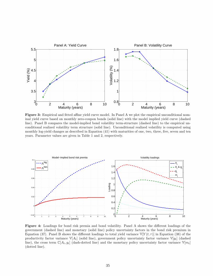
0 2 4 6 8 103
3.5
4
4.5
5
5.5Panel A: Yield Curve
Maturity (years)
Yie
ld (
%)
0 2 4 6 8 100.8
1
1.2
1.4
1.6
1.8Panel B: Volatility Curve
Vol
atili
ty (
%)
Maturity (years)
Figure 3: Empirical and fitted affine yield curve model. In Panel A we plot the empirical unconditional nom-inal yield curve based on monthly zero-coupon bonds (solid line) with the model implied yield curve (dashedline). Panel B compares the model-implied bond volatility term-structure (dashed line) to the empirical un-conditional realized volatility term structure (solid line). Unconditional realized volatility is computed usingmonthly log-yield changes as described in Equation (41) with maturities of one, two, three, five, seven and tenyears. Parameter values are given in Table 1 and 2, respectively.
0 1 2 3 4 5 6 7 8 9 10−0.02
0
0.02
0.04
0.06
0.08
0.1
Maturity (years)
Model−implied bond risk premia
ΛNg
ΛNm
0 2 4 6 8 100
0.2
0.4
0.6
0.8
1
1.2
1.4
1.6
Volatility loadings
Maturity (years)
Load
ing
At
At & g
t
gt
mt
Figure 4: Loadings for bond risk premia and bond volatility. Panel A shows the different loadings of thegovernment (dashed line) and monetary (solid line) policy uncertainty factors in the bond risk premium inEquation (37). Panel B shows the different loadings to total yield variance V[Y (t, τ)] in Equation (38) of theproductivity factor variance V[At] (solid line), government policy uncertainty factor variance V[gt] (dashedline), the cross term C[At, gt] (dash-dotted line) and the monetary policy uncertainty factor variance V[mt](dotted line).
35
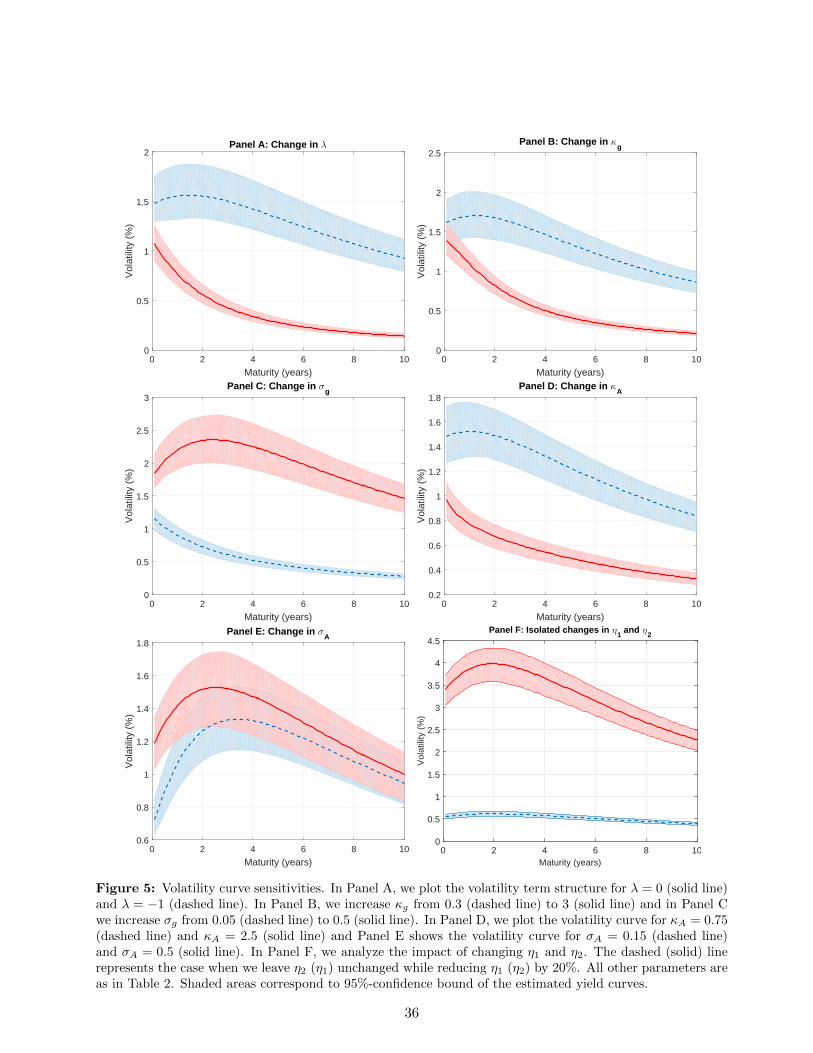
0 2 4 6 8 10
Maturity (years)
0
0.5
1
1.5
2
Vol
atili
ty (
%)
Panel A: Change in λ
0 2 4 6 8 10
Maturity (years)
0
0.5
1
1.5
2
2.5
Vol
atili
ty (
%)
Panel B: Change in κg
0 2 4 6 8 10
Maturity (years)
0
0.5
1
1.5
2
2.5
3
Vol
atili
ty (
%)
Panel C: Change in σg
0 2 4 6 8 10
Maturity (years)
0.2
0.4
0.6
0.8
1
1.2
1.4
1.6
1.8
Vol
atili
ty (
%)
Panel D: Change in κA
0 2 4 6 8 10
Maturity (years)
0.6
0.8
1
1.2
1.4
1.6
1.8
Vol
atili
ty (
%)
Panel E: Change in σA
Maturity (years)0 2 4 6 8 10
Vol
atili
ty (
%)
0
0.5
1
1.5
2
2.5
3
3.5
4
4.5Panel F: Isolated changes in η
1 and η
2
Figure 5: Volatility curve sensitivities. In Panel A, we plot the volatility term structure for λ = 0 (solid line)and λ = −1 (dashed line). In Panel B, we increase κg from 0.3 (dashed line) to 3 (solid line) and in Panel Cwe increase σg from 0.05 (dashed line) to 0.5 (solid line). In Panel D, we plot the volatility curve for κA = 0.75(dashed line) and κA = 2.5 (solid line) and Panel E shows the volatility curve for σA = 0.15 (dashed line)and σA = 0.5 (solid line). In Panel F, we analyze the impact of changing η1 and η2. The dashed (solid) linerepresents the case when we leave η2 (η1) unchanged while reducing η1 (η2) by 20%. All other parameters areas in Table 2. Shaded areas correspond to 95%-confidence bound of the estimated yield curves.
36
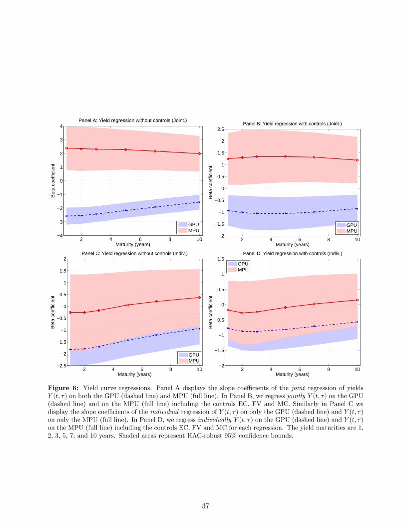
2 4 6 8 10−4
−3
−2
−1
0
1
2
3
4
Maturity (years)
Bet
a co
effic
ient
Panel A: Yield regression without controls (Joint.)
GPUMPU
2 4 6 8 10−2
−1.5
−1
−0.5
0
0.5
1
1.5
2
2.5
Maturity (years)
Bet
a co
effic
ient
Panel B: Yield regression with controls (Joint.)
GPUMPU
2 4 6 8 10−2.5
−2
−1.5
−1
−0.5
0
0.5
1
1.5
2
Maturity (years)
Bet
a co
effic
ient
Panel C: Yield regression without controls (Indiv.)
GPUMPU
2 4 6 8 10−2
−1.5
−1
−0.5
0
0.5
1
1.5
Maturity (years)
Bet
a co
effic
ient
Panel D: Yield regression with controls (Indiv.)
GPUMPU
Figure 6: Yield curve regressions. Panel A displays the slope coefficients of the joint regression of yieldsY (t, τ) on both the GPU (dashed line) and MPU (full line). In Panel B, we regress jointly Y (t, τ) on the GPU(dashed line) and on the MPU (full line) including the controls EC, FV and MC. Similarly in Panel C wedisplay the slope coefficients of the individual regression of Y (t, τ) on only the GPU (dashed line) and Y (t, τ)on only the MPU (full line). In Panel D, we regress individually Y (t, τ) on the GPU (dashed line) and Y (t, τ)on the MPU (full line) including the controls EC, FV and MC for each regression. The yield maturities are 1,2, 3, 5, 7, and 10 years. Shaded areas represent HAC-robust 95% confidence bounds.
37
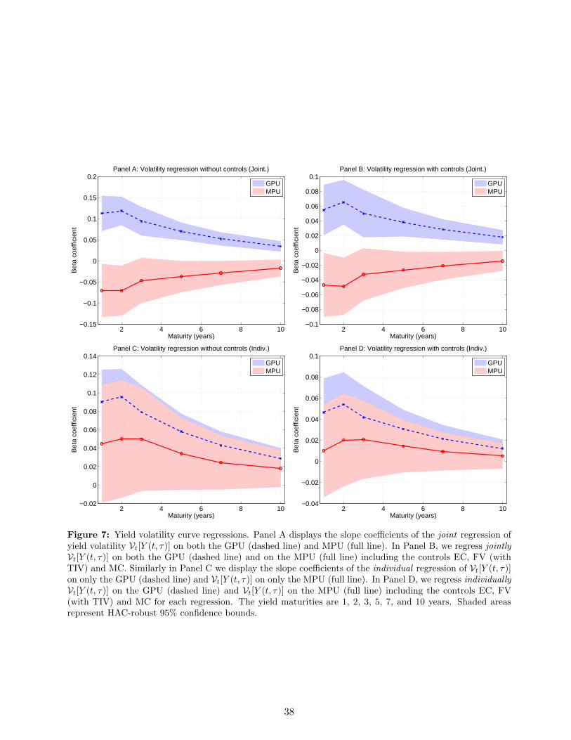
2 4 6 8 10−0.15
−0.1
−0.05
0
0.05
0.1
0.15
0.2
Maturity (years)
Bet
a co
effic
ient
Panel A: Volatility regression without controls (Joint.)
GPUMPU
2 4 6 8 10−0.1
−0.08
−0.06
−0.04
−0.02
0
0.02
0.04
0.06
0.08
0.1
Maturity (years)
Bet
a co
effic
ient
Panel B: Volatility regression with controls (Joint.)
GPUMPU
2 4 6 8 10−0.02
0
0.02
0.04
0.06
0.08
0.1
0.12
0.14
Maturity (years)
Bet
a co
effic
ient
Panel C: Volatility regression without controls (Indiv.)
GPUMPU
2 4 6 8 10−0.04
−0.02
0
0.02
0.04
0.06
0.08
0.1
Maturity (years)
Bet
a co
effic
ient
Panel D: Volatility regression with controls (Indiv.)
GPUMPU
Figure 7: Yield volatility curve regressions. Panel A displays the slope coefficients of the joint regression ofyield volatility Vt[Y (t, τ)] on both the GPU (dashed line) and MPU (full line). In Panel B, we regress jointlyVt[Y (t, τ)] on both the GPU (dashed line) and on the MPU (full line) including the controls EC, FV (withTIV) and MC. Similarly in Panel C we display the slope coefficients of the individual regression of Vt[Y (t, τ)]on only the GPU (dashed line) and Vt[Y (t, τ)] on only the MPU (full line). In Panel D, we regress individuallyVt[Y (t, τ)] on the GPU (dashed line) and Vt[Y (t, τ)] on the MPU (full line) including the controls EC, FV(with TIV) and MC for each regression. The yield maturities are 1, 2, 3, 5, 7, and 10 years. Shaded areasrepresent HAC-robust 95% confidence bounds.
38

2 3 4 5 6 7 8 9 10−4
−3
−2
−1
0
1
2
3
4
5
6
Maturity (years)
Bet
a co
effic
ient
Panel A: Bond risk premia regression without controls (Joint.)
GPUMPU
2 3 4 5 6 7 8 9 10−0.5
0
0.5
1
1.5
2
2.5
3
Maturity (years)
Bet
a co
effic
ient
Panel B: Bond risk premia regression with controls (Joint.)
GPUMPU
2 3 4 5 6 7 8 9 10−1
0
1
2
3
4
5
6
Maturity (years)
Bet
a co
effic
ient
Panel C: Bond risk premia regression without controls (Indiv.)
GPUMPU
2 3 4 5 6 7 8 9 10−0.5
0
0.5
1
1.5
2
2.5
3
3.5
Maturity (years)
Bet
a co
effic
ient
Panel D: Bond risk premia regression with controls (Indiv.)
GPUMPU
Figure 8: Bond risk premium regressions. Panel A displays the slope coefficients of the joint regression ofthe monthly excess returns rE,τit+1 on both the GPU (dashed line) and MPU (full line). In Panel B, we regress
jointly rE,τit+1 on both the GPU (dashed line) and on the MPU (full line) including the controls CP, PCA,EC, FV and MC for each regression. Similarly in Panel C we display the slope coefficients of the individualregression of the monthly excess returns rE,τit+1 on the GPU (dashed line) and the monthly excess returns rE,τit+1
on the MPU (full line). In Panel D, we regress individually the monthly excess returns rE,τit+1 on the GPU
(dashed line) and the monthly excess returns rE,τit+1 on the MPU (full line) including the controls CP, PCA, EC,FV and MC for each regression. The yield maturities are 1, 2, 3, 5, 7, and 10 years. Shaded areas representHAC-robust 95% confidence bounds.
39
A Proofs
A.1 Proof of Proposition 1
Proof. We start by deriving an n-th order recursive moment formula for the expectation of the
government policy uncertainty process gt with dynamics
dgt = κg (θg − gt) dt+ σg√gtdW
gt (A.1)
To compute its moments, let f(g) = gn where n ∈ N, then an application of Ito’s lemma and using
Equation (A.1) gives
dgnt = ngn−1t dgt +
1
2n(n− 1)gn−2
t σ2ggtdt (A.2)
=(−nκggnt + gn−1
t (nκgθg +n
2(n− 1)σ2
g))dt+ ngn−1
t σg√gtdW
gt
Integrating from t to T , taking expectations on both sides, using Fubini’s theorem and the law of
iterated expectation, differentiating with respect to T gives
ψ′t(T ) = Υ0(T ) + Υ1(T )ψt(T ) (A.3)
Υ0(T ) = Et[gn−1t+τ
] (nκgθg +
n
2(n− 1)σ2
g
)(A.4)
Υ1(T ) = −nκg (A.5)
Conditional on κg > 0, the solution to Equation (A.3) is
ψt(t+ τ) = eψ1τgnt +
∫ t+τ
tΥ0(t+ τ − u)eΥ1(t+τ−u)du (A.6)
Then the first moment satisfies
ψ′g(t, T ) :=
Et[gT ]
dT= κg(θg − Et[gT ]) (A.7)
ψg(t, t) := gt > 0 (A.8)
where Equation (A.8) represents the initial condition. The solution this fist order linear differential
equation in (A.7) can be represented as
ψg(t, T ) := Et[gT ] = θg + (gt − θg)e−κgτ (A.9)
40

and similarly, using Equation (A.9) one obtains that the second moment is given by
ψg2(t, T ) := Et[g2T ] = g2
t e−2κgτ +
(e−κgτ − e−2κgτ
)(2θgκg + σ2
g)
2κggt +
θg(2θgκg + σ2g) (1− e−κgτ )
2
2κg
ψg2(t, t) := g2t > 0
from which one can immediately deduce that the variance of gt is
Vt[gT ] = E[g2T ]− E[gT ]2 =
(2gt(e−κgτ − e−2κgτ
)+ θg (1− e−κgτ )
2)σ2g
2κg(A.10)
and its unconditional variance is
V[gt] =θgσ
2g
2κg(A.11)
Along the same line of argumentation, integrating Equation (5), applying Fubini’s theorem and the
law of iterated expectations we obtain that the conditional expected value of At satisfies
ψ′A(t, T ) :=
Et[AT ]
dT= κA (θA − ψA(t, T )) + λψg(t, T )
ψA(t, t) = At ∈ R (A.12)
where Equation (A.12) represents the initial condition for the process At. Using the expression for
ψg(t, T ) in Equation (A.9), the solution can be obtained using standard methods. Passing to the
limit, i.e., T →∞, gives the stationary expectation of At in Proposition 1. Next, in order to derive
the second moment of the productivity process At, we have to first derive the an expression for the
product expectation ψAg(t, T ) := Et [At+τgt+τ ]. An application of Ito’s formula to Atgt results in
the following dynamics
d (Atgt) =[(κAθA + ρAgσAσg
)gt + κAθAAt − (κA + κg)Atgt + λg2
t
]dt+ σAg
3/2t dWA
t + σgg3/2t dW g
t
Then, as above, integrating from t to T = t + τ , applying Fubini’s theorem and taking time t
conditional expectation shows that ψAg(t, T ) satisfies
ψ′Ag(t, T ) :=
Et[AT gT ]
dT=(κAθA + ρAgσAσg
)ψg(t, T ) + κAθAψA(t, T )− (κA + κg)ψAg(t, T ) + λψg2(t, T )
ψAg(t, t) = Atgt (A.13)
where Equation (A.13) represents the initial condition. Solving this first order differential equa-
tion with time-dependent functions ψg(t, T ), ψg2(t, T ) and ψA(t, T ) gives the conditional covariance
41
expression. Having obtained explicit conditional moments for At, gt and Atgt, the stationary co-
variance expression immediately follows from letting T → ∞, i.e. limT→∞ = Ct(At+τ , gt+τ ) =
Et[At+τ , gt+τ ]− Et[At+τ ]Et[gt+τ ]. Finally, by similar arguments as above and an application of Ito’s
formula to A2t we obtain that the second moment of At satisfies
ψ′
A2(t, T ) :=Et[A2
T ]
dT= 2κA (θA − ψA(t, T )) + 2λψAg(t, T ) + σ2
Aψg(t, T )ψg2(t, T )
ψA2(t, t) = A2t (A.14)
Solving this ordinary first order differential equation with time-dependent coefficients gives the ex-
pression for the conditional expectation of At. From Vt(At+τ ) = E[A2t+τ ] − E[At+τ ]2 and letting
T →∞ we immediately obtain the stationary variance expression for At.
A.2 Proof of Proposition 3
The optimal consumption and investment problem is
maxCs,Md
s
Et[∫ ∞
te−βsU(Cs,M
ds )dt
], (A.15)
where U(Ct,Mdt ) = 1
γ
((Ct(M
dt )ξ)γ − 1
)subject to the capital constraint in Equation (12). To
simplify notation, let Xt = (At, gt) such that the value function is given by
V = V (t,Kt, Xt) = maxCs,Md
s t≤s<∞Et[∫ ∞
te−βsU(Cs,M
ds )ds
]. (A.16)
In equilibrium, there exists a value function V (t,Kt, Xt) and control variables Ct,Mdt satisfying
the HJB equation
−∂V (t,Kt, Xt)
∂t= maxCt,Md
t
U(Ct,M
dt ) +AV (t,Kt, Xt)
. (A.17)
42
By standard time-homogeneity arguments for infinite horizon problems we have that
eβtV (t,Kt, Xt) = maxCs,Md
s t≤s<∞Et[∫ ∞
te−β(s−t)U(Cs,M
ds )ds
]= maxCt+u,Md
t+ut≤u<∞Et[∫ ∞
te−βuU(Ct+u,M
dt+u)du
]= maxCu,Md
u0≤u<∞E0
[∫ ∞0
e−βuU(Cu,Mdu)du
]≡ H(Kt, Xt), (A.18)
where the third equality follows because the optimal robust control is Markov and H(Kt, Xt) is
independent of time. Therefore, we conjecture that the value function has the following form
V (t,Kt, Xt) = a(t)H(Kt, Xt) =e−βt
βH(Kt, Xt) =
e−βt
βγ
((eφ(Xt)Kξ
t
)γ− 1), (A.19)
where φ : R2 → R is CN -differentiable function of the state vector Xt that needs to be determined in
equilibrium. Inserting (A.19) into the HJB equation in (A.17), the first order conditions are given
by
C∗t =Kt
(KQt e
φ(Xt))−γ
βQ
βQ(KQt e
φ(Xt))γ(− (γ−1)β
11−γ Q
11−γK
1−γQγ−1t e
γφ(Xt)1−γ
ξ
) 1−γγξ+γ−1
−ξKt
γγ−1
(A.20)
Md∗t =
(1− γ)β1
1−γQ1
1−γK1−γQγ−1
t eγφ(Xt)1−γ
ξ
1−γ
γξ+γ−1
, (A.21)
with Q = 1 + ξ. In general, the function φ(Xt) cannot be obtained in closed form. However, we can
obtain an asymptotic expansion to g(Xt) with respect to the risk aversion parameter γ. Assuming a
power series expression for φ(Xt) in γ as follows
φ(Xt) = φ0(Xt) + γφ1(Xt) +O(γ2),
where φ0(X, t) is obtained from the logarithmic utility case, we can then solve the HJB problem in
Equation (A.17) for γ 6= 0 in closed form. To do so, we solve first the HJB problem in the case where
utility of the representative agent is logarithmic.
43
A.2.1 Log-utility case
Note that for γ → 0 the utility reduces to
limγ→0
U(Ct,Mdt ) = log(Ct) + ξ log
(Mdt
). (A.22)
The optimal consumption and investment problem is38
maxCt,Md
t
E0
[∫ ∞0
e−βt[log(Ct) + ξ log
(Mdt
)]dt
], (A.23)
subject to the capital constraint in Equation (12). In equilibrium, there exists a value function
V log(t,Kt, Xt) = a(t)H log(Kt, Xt) and control variables Ct,Mdt satisfying the HJB equation
−∂(a(t)H log(Kt, Xt)
)∂t
= a(t)
(maxCt,Md
t
U log(Ct,M
dt ) +AH log(Kt, Xt)
). (A.24)
We consider the following linear conjecture for the value function V log(·)
a(t)H log(Kt, Xt) =e−βt
β[Q log(Kt) + g0(Xt)] , (A.25)
and where the function g(Xt) is affine in the state variables, i.e.,
φ(Xt) = φ00 + φ0AAt + φ0ggt. (A.26)
Applying the generator to Equation (A.25), using the productivity, the government policy, and
equilibrium capital accumulation dynamics in Equation (5), (6) and (20), we obtain
AV log =∂V log
∂t+∂V log
∂KµK +
∂V log
∂AµA +
∂V log
∂gµg +
1
2
∂2V log
∂K2σ2K
= Q
[µY + qAAt −
(CtKt
+Mdt
Kt
)− 1
2σ2Y gt
](A.27)
+ (κA (θA −At) + λgt)φ0A + κg (θg − gt)φ0g. (A.28)
The first order optimality conditions for consumption and money holdings are
e−βt
Ct− Q
β
e−βt
Kt= 0⇐⇒ C∗t =
βKt
Q, (A.29)
e−βtξ
Mdt
− Q
β
e−βt
Kt= 0⇐⇒Md∗
t =βξKt
Q. (A.30)
38The proof of this proposition is similar to the one presented in Buraschi & Jiltsov (2005).
44
Substituting the optimal controls C∗t and Md∗t into Equation (A.24) and matching coefficients of
log(Kt), At, gt and the constant terms, we obtain
Q = 1 + ξ (A.31)
and
φ00 =(1 + ξ)
(−θgκgσ2
Y (β + κA) + 2µY (β + κA)(β + κg) + 2θgκgλqA)
2β(β + κA)(β + κg)(A.32)
− (1 + ξ)(β(β + δ) + κA(β + δ − θAqA))
β(β + κA)+ L,
φ0A =(1 + ξ)qA(κA + β)
, φ0g =(1 + ξ)
(2λqAβ+κA
− σ2Y
)2(κg + β)
, (A.33)
where L is defined as
L = log
(β1+ξξξ
(1 + ξ)1+ξ
). (A.34)
The coefficients are all uniquely determined, state-independent and also independent of Kt. Substi-
tuting the expressions back into the HJB equations verifies that the guess was correct.
A.2.2 Perturbed solution
To derive an asymptotic approximation to the function φ(Xt), where the expansion taken with
respect to the risk aversion parameter γ, let V = V (t,Kt, Xt) denote the value function as given in
Equation (A.16). Utility is now given by the following non-separable preferences
U(Ct,Mdt ) =
1
γ
((Ct(M
dt )ξ)γ− 1). (A.35)
From the HJB equation in (A.17), the optimal consumption C∗t and money demand Md∗t policy
holdings are given by39
C∗t =(Mdt
)−ξQ(Mdt
)−ξ (KQt e
φ(Xt))γ
βKt
1
γ−1
, (A.36)
Md∗t =
(QC−γt KγQ−1
t eγφ(Xt)
βξ
) 1γξ−1
. (A.37)
39Inserting Equation (A.36) into (A.37) gives the optimal money demand in Equation (A.21) from which the optimalconsumption in Equation (A.20) can easily be deduced.
45
Inserting optimal money demand (A.37) into the first order condition of consumption (A.36), using
the power series representation of g(Xt) as given in Equation (18) and perturbing the resulting
expression around the log-utility case (and analogously for optimal money demand), substituting
Q = 1 + ξ from Equation (A.31), the perturbed optimal consumption and money holdings are given
by
C∗,Pt =βKt
(1 + ξ)
[1 + γ
(log
(β1+ξξξ
(1 + ξ)1+ξ
)− φ0(Xt)
)]+O(γ2), (A.38)
Md∗,Pt =
βξKt
(1 + ξ)
[1 + γ
(log
(β1+ξξξ
(1 + ξ)1+ξ
)− φ0(Xt)
)]+O(γ2). (A.39)
There are a number of important conclusions that can be drawn from the optimal perturbed solutions
in Equations (A.38) and (A.39). First, both equations only depend on φ0(Xt) and do not depend on
φ1(Xt) which implies that solving the consumption-investment problem with log-utility is sufficient to
fully characterize the optimal perturbed consumption and money holdings up to first order. Secondly,
C∗,Pt and Md∗,Pt are affine functions not only of capital Kt but also of the state vector Xt. This
property of the solution will not only render the equilibrium path process of Kt affine, but also
implies that optimal inflation dp∗t /p∗t remain affine in the state variables. Next, substituting C∗,Pt
and Md∗,Pt into Equation (13) immediately gives the equilibrium capital process K∗t in Equation
(20). To show the equilibrium price dynamics in (21), we apply Ito’s lemma to the money market
clearing condition MSt = p∗tM
d∗t and obtain40
dMSt = M∗dt dp∗t + p∗tdM
d∗t + Ct
(dp∗t , dM
∗dt
). (A.40)
Then using the optimal controls C∗t and Md∗t and inserting the money market clearing condition
from Equation (A.40) yields
dp∗tp∗t
=dMS
t
MSt
− dK∗tK∗t− Ct
(dp∗tp∗t
dK∗tK∗t
). (A.41)
Inserting the money supply rule of Equation (14) and the equilibrium capital accumulation process
into (A.41) gives the equilibrium price process as in Equation (21). To verify that the guess for the
value function V (·) was correct, we substitute the equilibrium values back into the HJB problem in
Equation (A.17).
40Assuming that at t = 0 markets are cleared. Hence, p∗0Md∗0 = MS
0 .
46
A.3 Proof of Proposition 4
To simplify notation, let κ∗t = log(K∗t ) +βt. The using the equilibrium capital accumulation process
implies that κ∗t satisfies
dκ∗t =
(µy + qAAt − δ −
1
2σ2Y gt + βγ (g0(Xt)− L)
)dt+ σY
√gtdW
Yt . (A.42)
The Euler condition in Equation (24) can then be expressed as
B(t, τ) = e−βτEt
[UC(C∗t+τ ,M
d∗t+τ )
UC(C∗t ,Md∗t )
p∗tp∗t+τ
]= e−βτEt
[K∗tK∗t+τ
p∗tp∗t+τ
]= e−βτEt
[exp− log
(K∗t+τ
)
exp− log (K∗t )p∗tp∗t+τ
]
= Et
[exp−
(log(K∗t+τ
)+ β(t+ τ)
)
exp− (log (K∗t ) + βt)p∗tp∗t+τ
]= Et
[exp−κ∗t+τexp−κ∗t
p∗tp∗t+τ
]. (A.43)
To solve the problem in Equation (A.43) we follow Ulrich (2013) and Buraschi & Jiltsov (2005) and
define
f = f(κ∗t , p∗t , At, gt,mt, τ) = Et
[e−κ
∗t+τ
p∗t+τ
]. (A.44)
Then, conjecturing a log-linear guess for f(·) of the form
f(κ∗t , p∗t , At, gt,mt, τ) =
e−κ∗t
p∗texp −b0(τ)− bA(τ)At − bg(τ)gt − bm(τ)mt . (A.45)
If our log-linear guess in Equation (A.45) solves the stochastic problem in (A.44) then it is also the
solution to the following PDE
−∂f(·, τ)
∂τ= Af(·, τ), f(·, 0) =
e−κ∗t
p∗t. (A.46)
The left-hand side of Equation (A.46) is given by
∂f(·, τ)
∂τ=[−b′0(τ)− b′A(τ)At − b
′g(τ)gt − b
′m(τ)mt
]f(·, τ). (A.47)
Setting Θ = κ∗t , p∗t , At, gt,mt, an application of Ito’s lemma to the right-hand side of (A.46) gives
Af(κ∗t , p∗t , At, gt,mt, τ) =
∑i∈Θ
∂f
∂ΘiµΘidt+
1
2
∑i∈Θ
∂2f
∂Θi2d〈Θi,Θi〉t +
∑i,j∈Θi 6=j
∂2f
∂ΘiΘjd〈Θi,Θj〉t. (A.48)
47

Writing out the expression above, recalling that ρgm = ρAg = ρMA = ρMg = 0 and substituting the
dynamics of κ∗t , p∗t , At, gt, and mt, we get
Af =∂f
∂κ∗
(µK∗ (At, gt)−
1
2σ2Y gt
)+∂f
∂p∗tp∗t
[µM − η1k − η2π
1− η2+η1 − 1
1− η2µK∗ (At, gt)− gt
(η1 − 1)σ2Y
1− η2
]+∂f
∂A(κA(θA −At) + λgt) +
∂f
∂gκg(θg − gt) +
∂f
∂mκm(θm −mt)
+1
2
[∂2f
∂κ∗2σ2Y gt +
∂2f
∂p∗2p∗2t
[gt
(η1 − 1
1− η2
)2
σ2Y +mt
σ2M
(1− η2)2
]
+∂2f
∂A2σ2Agt +
∂2f
∂g2σ2ggt +
∂2f
∂m2σ2mmt
]+
∂2f
∂κ∗∂p∗p∗tσ
2Y gt
η2 − 1
1− η2+
∂2f
∂κ∗∂AσAσY ρ
AY gt +∂2f
∂κ∗∂gσgσY ρ
gY gt
+∂2f
∂p∗∂Ap∗tη1 − 1
1− η2σAσY gtρ
AY +∂2f
∂p∗∂gp∗tη1 − 1
1− η2σgσY gtρ
gY .
Computing the derivatives and separating variables one obtains the following system of first order
asymptotic (Riccati) ODE’s:
0 = −CA + κAbA(τ) + b′A(τ), (A.49)
0 = Z0g(τ) + bg(τ)Z1g(τ) + Z2gb2g(τ) + b
′g(τ), (A.50)
0 = Z0m + bm(τ)Z1m + Z2mb2m(τ) + b
′m(τ), (A.51)
0 = −b′0(τ) + C0(τ) (A.52)
48
subject to bA(0) = bg(0) = bm(0) = b0(0) = 0 and where
CA = (qA + γβφ0A)
(η1 − η2
1− η2
), (A.53)
Z0g(τ) =(q2A + 2γβφ0A
)(η1 − η2
1− η2
)2 (1− e−κAτ )2σ2A
2κ2A
+(η1 − η2)2σ2
Y
(η2 − 1)2+ γ
βφ0g(η1 − η2)
η2 − 1
− bA(τ)
((η2 − 1)λ+ (η1 − η2)ρAY σAσY
η2 − 1
), (A.54)
Z1g(τ) = κg + bA(τ)ρAgσAσg +(η2 − η1)ρgY σgσY
η2 − 1, (A.55)
Z2g = σ2g/2, Hg(τ) =
√4Z0g(τ)Z2g − Z2
1g, (A.56)
Z0m =σ2M
(η2 − 1)2, Z1m = κm +
ρMmσmσM1− η2
, Z2m =σ2m
2, Hm =
√4Z0mZ2m − Z2
1m, (A.57)
C0(τ) =(µY − β − δ − k)η1 + β + µM − η2(µY + π − δ)
1− η2
+∑
i∈A,g,m
bi(τ)θiκi + γβ(η1 − η2)(L− φ00)
η2 − 1. (A.58)
For the existence of a solution to the bond pricing PDE that excludes arbitrage opportunities, requires
that the Riccati equations in (A.50) and (A.51) above, satisfy the following periodicity condition
4Z0g(τ)Z2g − Z21g(τ) < 0, 4Z0mZ2m − Z2
1m < 0, ∀ τ ≥ 0. (A.59)
This condition essentially rules out singularities of the solution of the Riccati equation above, i.e.,
for τ ≥ 0, the function bi(τ), i ∈ g,m is continuous in τ .
A.4 Proof of Proposition 5
The unconditional correlation coefficient of the nominal yield curve Y (t, τ) and gt is given by
% [Y (t, τ), gt] =C [Y (t, τ), gt]√V[Y (t, τ)]V[gt]
Using the affine expression in Equation (30) and the results from Proposition 1, the unconditional
covariance is
C[Y (t, τ), gt] =bA(τ)
τC[At, gt] +
bg(τ)
τV[gt] =
bA(τ)
τ
θgσg(2κgλρ
AgσA + λσg)
2κg(κA + κg)+bg(τ)
τ
θgσ2g
2κg,
49

where the unconditional variance of term structure is V[Y (t, τ)] =b2A(τ)
τ2V[At]+
b2g(τ)
τ2V[gt]+
b2m(τ)τ2
V[mt]+
2 bA(τ)τ
bg(τ)τ C [At, gt]. Along the same line of argumentation, we have that
C(Y (t, τ),mt) =θmσ
2m
2κm
bm(τ)
τ(A.60)
and since bm(τ) ≤ 0, τ ≥ 0 the result follows immediately.
A.5 Proof of Proposition 6
In this section we derive the first order asymptotic nominal short rate and the market prices of real
and nominal risks when the investor has CRRA utility. The nominal short rate is defined as the
following limit
Rt := limτ→0
Y (t, τ) = limτ→0−1
τ(log(B(t, τ))) . (A.61)
To prove Equation (34) we make repeated use of Bernoulli’s rule. For instance, to compute limτ→0b0(τ)τ
we set f(τ) :=∫ τ
0 C0(u)du and g(τ) = τ . Then, using Leibniz’ integral rule we obtain
limτ→0
f(τ)
g(τ)= lim
τ→0
f′(τ)
g′(τ)
= limτ→0
C0(τ) =(µY − β − δ − k)η1 + β + µM − η2(µY + π − δ)
1− η2+ γ
β(η1 − η2)(L− φ00)
η2 − 1,
Similarly we have
limτ→0
bA(τ)
τ= CA,
limτ→0
bg(τ)
τ= −Z0g(0) = −
((η1 − η2)2σ2
Y
(η2 − 1)2+ γ
βφ0g(η1 − η2)
η2 − 1
),
limτ→0
bm(τ)
τ= −Z0m = −
σ2M
(η2 − 1)2, (A.62)
which gives the expression for the short rate in Equation (34). Next, in order to derive the bond
excess return, we apply Ito’s rule to the closed-form bond price formula in Equation (25) and obtain
the following dynamics
dB(t, τ)
B(t, τ)=∂B(t, τ)
∂tdt+
∑i∈Θ
∂B(t, τ)
∂ΘidΘi
t +1
2
∑i∈Θ
∂2B(t, τ)
∂Θi2d〈Θi,Θi〉t, (A.63)
50
where Θ = A, g,m. Taking time t conditional expectation on both sides and using Equation (A.50)
and (A.51) from above, we obtain that the expected infinitesimal bond risk premia is given by
RP (t, τ) :=1
dtEt[dB(t, τ)
B(t, τ)−Rtdt
]=η2 − η1
η2 − 1σY[bA(τ)ρAY σA + σgbg(τ)ρgY
]gt + bm(τ)
σMσmρMm
η2 − 1mt,
(A.64)
which is after defining the nominal market price of risks the expression in Equation (37). The results
for the log-utility agent can be easily derived by simply setting γ = 0 in Proposition (6). However,
for verifying our results and to explain why we defined the market prices of government λN,Yt and
monetary policy risk λN,Mt as above, we derive both the nominal short rate, the market prices of risk
and the term premium from a different angle using the stochastic discount factor approach. Recall
that the real short rate can be obtained directly from the real stochastic discount factor which we
denote by ζRt . Its dynamics take the general form
dζRt = µ(ζR, t)dt+ σ(ζR, t)′dWt, (A.65)
where µ(·, ·) and σ(·, ·) are Ft-measurable bounded scalar drift and vector diffusion processes and
Wt = (W Yt ,W
Mt ). In our setup, ζRt = e−ρtUC(X∗t ) from which, after an application of Ito’s lemma
we finddζRtζRt
= −(µY + qAAt − δ − σ2
Y gt)dt− σy
√gtdW
Yt , (A.66)
from which we can read off the real short rate as rt = −µ(ζR, t) and the market price of the real
productivity innovation risk by λR,·t = σY√gt. Following Veronesi & Jared (2000) or Piazzesi &
Schneider (2006), the dynamics of the nominal stochastic discount factor ζNt are given by
−dζNt
ζNt=
µM + β(1− η1)− η1k − η2π − (η1 − η2)(δ − µY )
η2 − 1+qA(η1 − η2)
1− η2At
−(η1 − η2)2σ2
Y
(η2 − 1)2gt −
σ2M
(η2 − 1)2mt
dt+
(η1 − η2)σY1− η2
√gtdW
Yt +
σM1− η2
√mtdW
Mt , (A.67)
from which we deduce that Rt = −µ(ζN , t). Similarly we have that the nominal market prices of
risk is given by λN,·t = −σ(ζN , t). Next, in order to determine the term premium on nominal bond
yields under log-utility, we make use of the closed-form solution of the nominal bond price as given
in Proposition 4, and the nominal short rate together with the associated market prices λN,Yt and
λN,Mt as in Proposition 6. An application of Ito’s lemma to Equation (25) shows that the risk-neutral
51
dynamics of the bond price equals to
dB(t, τ)
B(t, τ)= Rtdt− bA(τ)σA
√gtdW
At − bg(τ)σg
√gtdW
gt − bm(τ)σm
√mtdW
mt , (A.68)
where W it , i ∈ A, g,m are Ft-measurable Brownian innovation processes under the risk neutral
measure Q. According to Proposition 4, only government and nominal monetary policy risk are
priced. We can decompose the Brownian innovations WAt , W
gt and Wm
t into two orthogonal com-
plements as follows
dWAt = ρAY dW Y
t +
√1− ρAY 2dWA
t , dW Yt dW
At = 0,
dW gt = ρY gdW Y
t +
√1− ρY g2dW g
t , dW Yt dW
gt = 0
dWmt = ρMmdWM
t +
√1− ρMm2dWm
t , dWMt dW Y
t = 0. (A.69)
Hence, substituting the decomposed Brownian motions into Equation (A.68), the bond price dynam-
ics are then given by
dB(t, τ)
B(t, τ)= Rtdt− bA(τ)σA
√gt
(ρAY dW Y
t +
√1− ρAY 2dWA
t
)− bg(τ)σg
√gt
(ρY gdW Y
t +
√1− ρY g2dW g
t
)− bm(τ)σm
√mt
(ρMmdWM
t +
√1− ρMm2dWm
t
).
Next, in order to express the bond under the physical measure P we apply Girsanov’s theorem to
perform a measure change from Q to P as follows. We set the change of the drift equal to the market
price of risk, in other words we have dW Yt = λN,Yt dt + dW Y
t and dWMt = λN,Mt dt + dWM
t . Then,
given the correlation structure of the factors we obtain that the equilibrium term premium under
the physical measure P is given by
1
dtEt[dB(t, τ)
B(t, τ)−Rtdt
]= λN,Yt
[bA(τ)ρAY σA + σgbg(τ)ρgY
]√gt − bm(τ)λN,Mt
√mt. (A.70)
52

B Supplementary Tables
EPU GPU MPU 1Y 2Y 3Y 5Y 7Y 10Y
EPU 1 0.857 0.657 -0.544 -0.542 -0.533 -0.500 -0.468 -0.425GPU 1 0.572 -0.450 -0.444 -0.435 -0.401 -0.369 -0.324MPU 1 -0.036 -0.037 -0.026 0.006 0.029 0.0561Y 1 0.993 0.982 0.952 0.927 0.8962Y 1 0.997 0.979 0.961 0.9363Y 1 0.991 0.979 0.9585Y 1 0.997 0.9877Y 1 0.99610Y 1.000
Table 6: Sample correlation matrix of EPU, GPU and MPU index with nominal yields with τ= 1Y, 2Y, 3Y,5Y, 7Y and 10Y using data from January 1990 until June 2014.
EPU GPU MPU 1Y 2Y 3Y 5Y 7Y 10Y
EPU 1 0.8573 0.6573 0.6272 0.6611 0.664 0.6533 0.6254 0.6048GPU 1 0.5724 0.4898 0.527 0.5211 0.5218 0.495 0.462MPU 1 0.1081 0.1236 0.1451 0.1309 0.1175 0.12431Y 1 0.9406 0.9214 0.8784 0.8497 0.82612Y 1 0.9887 0.9644 0.9381 0.90673Y 1 0.9815 0.9595 0.93355Y 1 0.9935 0.97287Y 1 0.987710Y 1
Table 7: Sample correlation matrix of EPU, GPU and MPU index with realized volatility as in Equation(41) with τ= 1Y, 2Y, 3Y, 5Y, 7Y and 10Y using data from January 1990 until June 2014.
τ 1Y 2Y 3Y 5Y 7Y 10Y
Full regression GPU 0.051 0.0558 0.05* 0.042** 0.032* 0.022**tGPU (2.89) (5.36) (5.37) (8.22) (8.03) (7.46)R2adj 0.69 0.81 0.80 0.83 0.83 0.83
Full Regression MPU 0.011 -0.012 0.011* 0.01** 0.007* 0.05**tMPU (1.11) (1.49) (1.67) (1.961) (1.91) (1.961)R2adj 0.65 0.76 0.75 0.76 0.76 0.77
Table 8: Summary of regression results: Table displays the slope coefficients of the regression of Vt[Y (t, τ)]on MPUt and GPUt individually, plus the economic condition controls (EC), the financial variables (FV)plus macro factors (RA and IF) for τ=1Y, 2Y, 3Y, 5Y, 7Y, and 10Y. Values in brackets below representHAC-robust t−statistics. R2
adj refers to adjusted coefficient of determination. By ***, **, * we denote 1%,5%, and 10% statistical significance, respectively.
53
References
Ang, A. & Piazzesi, M. (2003), ‘A no-arbitrage vector autoregression of term structure dynamics
with macroeconomic and latent variables’, Journal of Monetary Economics 50, 745–787.
Baker, S., Bloom, N. & Davis, S. J. (2012), ‘Measuring economic policy uncertainty’, Manuscript
Stanford University .
Balduzzi, P., Elton, E. & Green, T. (2001), ‘Economic news and bond prices: evidence from the u.s.
treasury market.’, Journal of Financial and Quantitative Analysis 36, 523–543.
Bansal, R. & Shaliastovich, I. (2013), ‘A Long-Run Risks Explanation of Predictability Puzzles in
Bond and Currency Markets’, Review of Financial Studies 26(1), 1–33.
URL: http://ideas.repec.org/a/oup/rfinst/v26y2013i1p1-33.html
Bansal, R. & Yaron, A. (2004), ‘Risks for the long run: A potential resolution of asset pricing
puzzles’, The Journal of Finance 59, 1481–1509.
Bauer, M. D. & Rudebusch, G. D. (2015), ‘Resolving the spanning puzzle in macro-finance term
structure models’.
Bekaert, G., Engstrom, E. & Xing, Y. (2009), ‘Risk, uncertainty, and asset prices’, Journal of
Financial Economics 91(1), 59–82.
Bekaert, G., Harvey, C. R., Lundblad, C. T. & Siegel, S. (2014), ‘Political risk spreads’, Journal of
International Business Studies 45(4), 471–493.
Belo, F., Gala, V. & Li, J. (2013), ‘Government spending, political cycles and the cross section of
stock returns’, Journal of Financial Economics 107, 305–324.
Bialkowski, J., Gottschalk, K. & Wisnieski, T. (2008), ‘Stock market volatility around national
elections’, Journal of Banking and Finance 32, 1941–1953.
Bloom, N. (2009), ‘The impact of uncertainty shocks’, Econometrica 77(3), 623–685.
Bond, P. & Goldstein, I. (2012), ‘Government intervention and information aggregation by prices’,
Working Paper .
54
Boutchkova, M. K., Doshi, H., Durnev, A. & Molchanov, A. (2012), ‘Precarious politics and return
volatility’, The Review of Financial Studies 25, 1111–1154.
Brogaard, J. & Detzel, A. (2012), ‘The asset pricing implications of government economic policy
uncertainty’, Working Paper .
Buraschi, A., Carnelli, A. & Whelan, P. (2014), ‘Monetary policy and treasury risk premia’, Working
Paper .
Buraschi, A. & Jiltsov, A. (2005), ‘Inflation risk premia and the expectation hypothesis’, Journal of
Financial Economics 75, 429–490.
Buraschi, A. & Jiltsov, A. (2007), ‘Habit formation and macroeconomic models of the term structure
of interest rates’, The Journal of Finance 6, 3009–30063.
Campbell, J. Y. & Shiller, R. J. (1991), ‘Yield spreads and interest rate movements: A bird’s eye
view’, Review of Economic Studies 58, 495–514.
Cochrane, J. & Piazzesi, M. (2005), ‘Bond risk premia’, American Economic Review 95, 138–160.
Cox, J., Iingersoll, J. & Ross, S. (1985), ‘A theory of the term structure of interest rates’, Econo-
metrica 53, 385–408.
David, A. & Veronesi, P. (2014), ‘Investors’ and central bank’s uncertainty embedded in index
options’, Review of Financial Studies 27(6), 1661–1716.
de Goeij, P. & Marquering, W. (2006), ‘Macroeconomic announcements and asymmetric volatility
in bond returns’, Journal of Banking and Finance 30(10), 2659–2680.
Duffie, D. & Kan, R. (1996), ‘A yield factor model of interest rates’, Mathematical Finance 6, 379–
406.
Durnev, A. (2010), ‘The real effects of political uncertainty: Elections and investment sensitivity to
stock prices’, Working Paper University of Iowa.
Evans, C. & Marshall, D. (2007), ‘Economic determinants of the nominal treasury yield curve’,
Journal of Monetary Economics 54, 1986–2003.
55

Fama, E. & French, K. (1989), ‘Business conditions and expected returns on stocks and bonds’,
Journal of Financial Economics 25, 23–49.
Fisher, S. & Modigliani, F. (1978), ‘Towards an understanding of the real effects and costs of infla-
tion’, Weltwirtschaftliches Archiv 114, 810–832.
Fleming, M. & Piazzesi, M. (2005), ‘Monetary policy tick-by-tick’, Working Paper .
Gallmeyer, M. F., Hollifield, B., Palomino, F. & Zin, S. E. (2007), Arbitrage-free bond pricing with
dynamic macroeconomic models, Working Paper 13245, National Bureau of Economic Research.
URL: http://www.nber.org/papers/w13245
Gurkaynak, R. S., Sack, B. & Swanson, E. (2005a), ‘Do actions speak louder than words? the
response of asset prices to monetary policy actions and statements’, International Journal of
Central Banking pp. 55–93.
Gurkaynak, R. S., Sack, B. & Swanson, E. (2005b), ‘The sensitivity of long-term interest rates to
economic news: Evidence and implications for macroeconomic models’, The American Economic
Review 95, 425–426.
Gulen, H. & Ion, M. (2012), ‘Policy uncertainty and corporate investment’, Working Paper .
Hansen, L. P., Heaton, J. C. & Li, N. (2008), ‘Consumption strikes back? measuring long?run risk’,
Journal of Political Economy 116(2), pp. 260–302.
Huang, T., Wu, F., Yu, J. & Zhang, B. (2015), ‘International political risk and government bond
pricing’, Journal of Banking and Finance 55, 393–405.
Joslin, S., Priebisch, M. & Singleton, K. (2014), ‘Risk premiums in dynamic term structure models
with unspanned macro risks’, The Journal of Finance 69, 1197–1233.
Joslin, S., Priebsch, M. & Singleton, K. J. (2014), ‘Risk Premiums in Dynamic Term Structure
Models with Unspanned Macro Risks’, Journal of Finance 69(3), 1197–1233.
URL: http://ideas.repec.org/a/bla/jfinan/v69y2014i3p1197-1233.html
56

Julio, J. & Yook, Y. (2012), ‘Political uncertainty and corporate investment cycles’, Journal of
Finance 67, 45–83.
Kelly, B., Pastor, L. & Veronesi, P. (2013), ‘The price of political uncertainty: Theory and evidence
from the option market’, Working Paper .
Kogan, L. & Uppal, R. (2001), Risk aversion and optimal portfolio policies in partial and general
equilibrium economies, Working paper, Sloan School of Management, MIT.
Kuttner, K. N. (2001), ‘Monetary policy surprises and interest rates: Evidence from the fed funds
futures market’, Journal of Monetary Economics 47, 523–544.
Litterman, R. B. & Scheinkman, J. (1991), ‘Common factors affecting bond returns’, The Journal
of Fixed Income 1, 54–61.
Ludvigson, S. & Ng, S. (2009), ‘Macro factors in bond risk premia’, Review of Financial Studies
22, 5027–5067.
Newey, W. & West, K. (1994), ‘Automatic lag selection in covariance estimation’, Review of Economic
Studies 61, 631–653.
Øksendal, B. (2003), Stochastic differential equations, Springer.
Pastor, L. & Veronesi, P. (2012), ‘Uncertainty about government policy and stock prices’, Journal
of Finance 4, 1219–1264.
Pastor, L. & Veronesi, P. (2013), ‘Political uncertainty and risk premia’, Journal of Financial Eco-
nomics 110, 520–545.
Pennacchi, G. (1991), ‘Identifying the dynamics of real interest rates and inflation evidence using
survey data’, The Review of Financial Studies 4, 53–86.
Piazzesi, M. (2005), ‘Bond yields and the federal reserve’, Journal of Political Economy 112, 311–344.
Piazzesi, M. & Schneider, M. (2006), ‘Equilibrium yield curves’, NBER Working Paper Series .
57
Pindyck, R. & Solimano, A. (1993), ‘Economic instability and aggregate investment’, NBER Working
Paper Series .
Rodrik, D. (1991), ‘Policy uncertainty and private investment in developing countries’, Journal of
Development Economics 36, 229–242.
Shiller, R. (1979), ‘The volatility of long-term interest rates and expectations models of the term
structure’, Journal of Political Economy 87, 1190–1219.
Ulrich, M. (2013), ‘Inflation ambiguity and the term structure of u.s. government bonds’, Journal of
Monetary Economics 60, 295–309.
Vasicek, O. (1977), ‘An equilibrium characterization of the term structure’, Journal of Financial
Economics 5, 177–188.
Veronesi, P. & Jared, F. (2000), ‘Short and long horizon term and inflation risk premia in the us
term structure’, Working Paper .
Wachter, J. A. (2006), ‘A consumption-based model of the term structure of interest rates’, Journal
of Financial economics 79(2), 365–399.
Wright, J. (2012), ‘What does monetary policy do to long-term interest rates at the zero lower
bound?’, The Economic Journal 122, 447–66.
Xiong, W. & Yan, H. (2010), ‘Heterogenous expectations and bond markets’, Review of Financial
Studies 23, 1433–1466.
58
Recommended