Earnings Announcements are Full of Surprises
Michael W. Brandta
Runeet Kishoreb
Pedro Santa-Clarac
Mohan Venkatachalamd
This version: January 22, 2008
Abstract
We study the drift in returns of portfolios formed on the basis of the stock price reaction around earnings announcements. The Earnings Announcement Return (EAR) captures the market reaction to unexpected information contained in the company’s earnings release. Besides the actual earnings news, this includes unexpected information about sales, margins, investment, and other less tangible information communicated around the earnings announcement. A strategy that buys and sells companies sorted on EAR produces an average abnormal return of 7.55% per year, 1.3% more than a strategy based on the traditional measure of earnings surprise, SUE. The post earnings announcement drift for EAR strategy is stronger than post earnings announcement drift for SUE. More importantly, unlike SUE, the EAR strategy returns do not show a reversal after 3 quarters. The EAR and SUE strategies appear to be independent of each other. A strategy that exploits both pieces of information generates abnormal returns of about 12.5% on an annual basis.
a Fuqua School of Business, Duke University, and NBER. (919) 660-1948, [email protected]. b Fuqua School of Business, Duke University, (919) 660-2942, [email protected]. c Anderson School of Business, UCLA, and NBER, (310) 206-6077, [email protected]. d Fuqua School of Business, Duke University, (919) 660-7859, [email protected]. We are grateful for financial support from the Fuqua School of Business, Duke University and Anderson School of Business, UCLA. We appreciate helpful comments from Qi Chen, Richard Mendenhall, Cathy Schrand and Richard Sloan.
1
Earnings Announcements are Full of Surprises
1. Introduction
Since Ball and Brown (1968), a number of studies have documented the post-earnings
announcement drift phenomenon where stock prices tend to drift upward (downward) after the
earnings announcement if the earnings are unexpectedly positive (negative). This drift
constitutes a violation of stock market efficiency and attempts to explain this phenomenon as an
artifact of omitted risk factors, mismeasured returns, or research design flaws have been only
partially successful. Thus, post earnings announcement drift continues to pose a significant
challenge to financial theorists (Brennan 1991; Fama 1998).
Our paper deepens the puzzle. Research up to now has primarily attempted to measure
the surprise in the announced earnings number. This surprise is the difference between the
realized earnings and an estimate of the investors’ expectation of earnings, either from a time
series model of earnings or from analyst forecasts. After standardizing this surprise by a
measure of earnings uncertainty, this measure is typically referred to as Standardized
Unexpected Earnings (SUE). We focus instead on the stock return around the time of the
announcement in excess of the return of a portfolio of firms with similar risk exposures and refer
to it as the Earnings Announcement Return, or EAR. When measured in a short window around
the announcement, the EAR is mainly driven by the unexpected information contained in the
announcement. Importantly, the EAR captures the surprise in all aspects of the company’s
earnings announcement, and not just the surprise in earnings. Besides earnings, firms disclose
sales and margins, and often release other forward-looking information in the form of press
releases, conference calls, or private communications around the earnings announcement date, all
of which will be impounded into stock prices at that time. As an additional advantage, EAR

2
does not suffer from estimation errors like SUE which requires an estimate of the market’s
unobservable expectation of earnings.
We define firms with extreme positive EAR (i.e., firms in the highest quintile of
unexpected returns) at the earnings announcement date as “good-news” firms and firms with
extreme negative EAR (i.e., firms in the lowest quintile of unexpected returns) as “bad-news”
firms. We find that returns tend to drift upward (downward) for good-news (bad-news) firms
over the subsequent four quarters. A trading strategy taking long positions in good-news stocks
and short positions in bad-news stocks produces an annual abnormal return of 7.5%. This return
is better than the 6.2% obtained in a similar trading strategy based on the traditional SUE
measure. Though the difference in returns is not large, it suggests that market participants under-
react to all the information in the earnings announcement and not just to the surprise in the
earnings number.
At first blush, the similar returns obtained for the EAR and SUE strategy might lead a
reader to conclude that these two strategies are not independent in that each of the strategies may
subsume the other. It turns out that it is not the case. We find that significant abnormal returns
obtain for the EAR strategy even after controlling for the SUE strategy, and vice-versa.
Therefore, investors under-react to both the earnings and the other information in the
announcement, and one effect does not subsume the other. In other words, the two strategies are
largely independent. A trading strategy that combines the two signals significantly improves the
magnitude of abnormal returns to 12.5% per year.
Furthermore, the pattern of returns generated by the EAR and SUE strategies is quite
different. While both the SUE strategy and EAR strategy cumulative abnormal returns increase
monotonically across the four quarters subsequent to portfolio formation, the SUE strategy

3
registers a decline in the fourth quarter. This is partly due to the reversal in SUE strategy stock
returns surrounding the earnings announcement date four quarters after the portfolio formation
(see Bernard and Thomas 1990). Another important distinction between the EAR and SUE
strategies is that the abnormal returns from the EAR strategy have increased over time, while the
abnormal returns from the SUE strategy have dropped since 1996. This is consistent with
Francis, Schipper and Vincent (2002) who document the increasing concurrent disclosures of
other information during earnings announcements over the last decade. It is, of course, also
consistent with the SUE effect being exploited by savvy investors who, by their actions, have
arbitraged away a significant portion of the anomaly.
The cumulative abnormal returns across time for both the SUE and EAR strategy appear
to be drifting. We interpret this finding as suggesting that earnings and non-earnings surprises
are confirmed continuously throughout the next quarters and, as this happens, stock prices drift
upward or downward depending on the sign of the initial surprise. This is consistent with
findings in Soffer and Lys (1999) that investors appear to discern more information about future
earnings as time progresses and new information arrives. It appears investors follow a similar
inference process for valuation factors unrelated to earnings as well.
Foster, Olsen and Shevlin (1984) and Chan, Jegadeesh and Lakonishok (1996) also use
announcement day abnormal returns. However, our paper is different from these two papers in
several respects. Foster et al. (1984) use a slightly different measure of announcement day
returns in that they scale the returns by the standard deviation of returns to be consistent with the
SUE measure. Using this measure they are unable to document any subsequent return patterns.
Chan et al. (1996) use a measure similar to ours but the focus of their paper is quite different.
Their objective was to understand price momentum and its relation to post earnings
4
announcement drift and they used earnings announcement returns as a proxy for earnings
surprises. In contrast, we argue that the earnings announcement return is not merely a proxy for
the earnings surprise; rather it combines two important and distinct pieces of information
surrounding the earnings release, i.e., earnings and non-earnings information. Furthermore,
Chan et al. (1996) do not analyze the subsequent return patterns based on SUE and EAR
measures, which is the focus of our paper. Finally, we report how the return patters emerge
when combining the SUE and EAR measures.
Our paper offers three contributions to the extant literature. First, we add to the literature
on drifts by documenting that the market under-reaction to information at the earnings
announcement date extends beyond the earnings news. Second, we contribute to the literature
that examines the valuation implications of non-financial information. While prior research
consistently documents an association between non-financial information and stock prices it is
often unclear whether market participants correctly value this piece of information. The
evidence presented here adds to the growing body of work that suggests this is not the case
(Rajgopal, Shevlin and Venkatachalam 2003, Gu 2005). Third, we shed light on an anomaly that
is more pervasive and generates greater abnormal returns than the post earnings announcement
drift anomaly. It is intriguing that such a visible piece of information, the announcement return,
can lead to predictable returns in the future. While the post earnings announcement drift can be
at least partially explained by the lack of understanding of the time-series properties of earnings,
it is unclear what might explain the drift following the announcement return.
The rest of the paper is organized as follows. In section 2, we discuss related research.
Section 3 describes the sample while section 4 presents the empirical methodology and findings.
5
We present some concluding remarks in section 5.
2. Related research
Ball and Brown (1968) discovered the post earnings announcement drift over three
decades ago but it still remains a puzzle as the drift persists even after years of research and
public dissemination of the anomaly. An extensive body of literature has attempted to explain
the drift as compensation for some risk factor or due to methodological flaws, but such
endeavors have been largely unsuccessful (see Bernard, Thomas and Whalen 1997 for a
discussion).
Bernard and Thomas (1990) and Ball and Bartov (1996), among others, show that
investors’ apparent inability to fully process the time-series properties of earnings is a plausible
explanation for the drift. That is, investors fail to fully recognize the serial correlation in
quarterly earnings shocks, and, as such, systematically misestimate future expected earnings.
Consequently, when subsequent quarterly earnings are announced, stock prices respond to a
component of the earnings that is a surprise even though it should have been predictable based
on the past time series of earnings.
Prior research has predominantly focused on the earnings surprise and very little attention
has been directed towards other non-earnings information (both financial and non-financial in
nature) that is concurrently released around the earnings announcement date. Firms provide
considerable information in press releases both elaborating on the earnings report as well as
providing other forward looking information. For example, firms provide expanded information
about components of earnings such as sales and operating margin or report forward looking
information such as order backlog data. In addition, earnings-related conference calls that are
6
typically held within a few hours of the earnings announcement have become increasingly
common. These conference calls represent an important voluntary disclosure mechanism for
firms to disseminate valuable information to analysts and investors. Moreover, analysts obtain
soft information about future firm performance in private discussions with the firm management
(Hutton 2005).1 Thus, market participants become aware of significant pieces of new
information in addition to earnings at the earnings announcement date. For example, Francis et
al. (2002) examine press releases for a sample of firms during the period 1980-1999 and find a
considerable increase in the length of the press releases (measured by the number of words) as
well as the number of items disclosed. They also document that this increase in concurrent
disclosures helps explain the increase in the absolute market reaction to earnings announcements.
It is therefore reasonable to argue that the market returns surrounding the earnings release
reflects both earnings and non-earnings information released on the announcement. More
importantly, it appears that the proportion of market reaction attributable to non-earnings
information is on the rise.
The lack of explanatory power of unexpected earnings for the returns around the
announcement documented by the accounting literature (see Lev 1989 for a review) is also
consistent with the arguments above. Recent research by Liu and Thomas (2000) shows that a
significant portion of the market reaction surrounding earnings announcements is attributable to
other information released around the announcement date rather than the earnings information
itself. Thus, a natural question to examine is whether market participants correctly impound into
share prices the other information that is concurrently disclosed at the earnings release.
1 The promulgation of Regulation FD in Aug 2000 by the SEC curbed the practice of selective disclosure of material information. While critics claimed that this regulation might result in less disclosures, recent research by Bushee et al. (2004) finds otherwise.
7
Recent research that examines whether market participants are able to correctly value the
future earnings implications of nonfinancial information finds conflicting results. For example,
Rajgopal, Shevlin and Venkatachalam (2003) find that investors overestimate the valuation
implications of order backlogs that are disclosed in the financial statements. That is, investors
place a higher weight on order backlog than that implied by the association between order
backlog and future earnings. A trading strategy that takes a long (short) position in the lowest
(highest) decile of order backlog generates significant future abnormal returns. In contrast, Gu
(2005) finds that changes in patent citations have positive implication for future earnings but
investors generally treat them as if they contained no relevant information. In other words,
investors underweight the value implications of changes in patent citation. Deng, Lev and Narin
(1999) document a similar underweighting of patent counts and level of patent citations. Thus,
there is no consistent evidence of investor over or under reaction to non-financial information.
Furthermore, none of these studies examine the short-run pricing implications of other
information disclosed surrounding earnings announcements. Also, these papers focus on a single
non-financial indicator such as order backlog, patent count, or patent impact, and hence limit the
generalizability of their findings to a broader set of information. Our paper extends this literature
by examining whether market participants under or over react to a broader set of concurrent
disclosures at earnings announcements.
In a paper most directly related to ours, Chan et al. (1996) use the stock returns
surrounding the earnings announcement as an alternative measure (to standardized unexpected
earnings) of the post earnings announcement drift phenomenon to study its relationship with
price momentum. Using both measures they document that the post earnings announcement drift
still persists even after controlling for price momentum. Unlike Chan et al. (1996) we treat these
8
measures as capturing different elements of the information around earnings announcement.
Thus, our paper extends their work by examining whether the subsequent return patterns
attributable to the two alternative measures are different. In particular, we are interested in the
interactions between these two measures to gain a better understanding of the subsequent returns
attributable to surprises in earnings and non-earnings news.
3. Data and methodology
Our data spans January 1987 to December 2004. Our sample consists of firms reported
on COMPUSTAT Industrial Quarterly and CRSP databases and for which we can calculate size
and book-to-market ratios. We do not include financials (NAICS 2-digit code 52) and utilities
(NAICS 2-digit code 22) in our sample.2 We also exclude firms with CRSP daily price less than
$5 on the trading day prior to the earnings announcement date (COMPUSTAT Data RDQE). The
Standardized Unexpected Earnings, SUE, for a firm in a given quarter is constructed by dividing
the earnings surprise by the standard deviation of earnings surprises:
qi
qiqiqi
XEXSUE
,
,,,
)(σ−
= , (1)
where qiX , (COMPUSTAT Data 8) is the actual earnings number for firm i in quarter q, )( ,qiXE
the expected earnings counterpart and qi,σ the standard deviation of earnings surprises over the
last eight quarters.
Following previous research (e.g., Bernard and Thomas 1990), a seasonal random walk
with drift model is used to estimate expected earnings. More specifically:
2 Including these firms does not alter our inferences. In particular, a combined SUE and EAR strategy that includes utilities and financial firms results in an abnormal return of 12.1% over a 240 day trading window comparable to the 12.48% return obtained without including these firms (see Table 3).

9
qiqiqi XXE ,4,, )( μ+= − (2)
8
8
14,,
,
∑=
−−− −= n
nqinqi
qi
XXμ . (3)
In Section 4.4, we show that our main findings are robust to the use of consensus analyst
forecasts from I/B/E/S as an alternative measure of earnings expectation.
We use an alternative and arguably broader measure of the surprise in an earnings
announcement, that we term the Earnings Announcement Return, EAR. EAR is the abnormal
return for firm i in quarter q recorded over a three-day window centered on the announcement
date:
∏∏+
−=
+
−=
+−+=1
1
1
1,, )1()1(
t
tjj
t
tjjiqi FFREAR , (4)
where jFF is the return on the benchmark size and book-to-market Fama-French portfolio to
which stock i belongs. Following Fama and French (1992), we form six portfolios based on the
intersection of two size-based cutoffs and three book-to-market based cutoffs. jiR , is the return
on stock i on date j surrounding the earnings announcement in quarter q.
For every quarter, we form portfolios as follows:
a) We calculate SUE and EAR for all the stocks in the COMPUSTAT Industrial Quarterly files
as described in equations (1) through (4).
b) We calculate quintile breakpoints by ranking SUE or EAR observations from quarter q-1
rather than quarter q. This mitigates potential look-ahead bias associated with ranking
observations based on quarter q realizations of SUE and EAR. That is, because the return
accumulation starts a day after the earnings announcement in quarter q, it is not practically

10
feasible to ascertain whether a firm falls in the extreme positive or negative surprises
quintiles until all firms announce their earnings for quarter q.
c) We form 5 portfolios based on SUE, 5 portfolios based on EAR, and 25 portfolios (two-way
SUE × EAR independent sort) and examine abnormal returns to each of those portfolios in
subsequent periods.
Each quarter, we also analyze cumulative post announcement returns for both EAR and SUE
strategies. Returns start cumulating a day after the earnings announcement window ends and
cumulate up to n days after the earnings announcement date. For example, if t is the earnings
announcement date for a stock, returns are cumulated from t+2 through t+n trading days. This
cumulative return is the n day cumulative return for the given stock. The n day cumulative
abnormal returns are calculated using
)1()1(2 2
,, ∏ ∏+
+=
+
+=
+−+=nt
tj
nt
tjjjini FFRABR (5)
4. Empirical results
The fundamental hypothesis of our paper is that pieces of information in addition to
earnings arrive around the earnings announcement date and that a significant portion of the
market reaction around the announcement date is attributable to non-earnings information. To
investigate this hypothesis, we first examine the distribution of returns around the earnings
announcement date across different quintiles of both EAR and SUE, independently of each other.
The abnormal returns to a strategy based on perfect foresight of extreme good news and bad
news in earnings (i.e., perfect foresight of SUE) is 3.41% (see Panel A of Table 1). In contrast,
the average abnormal return to a strategy based on perfect foresight of good news and bad news
as measured through the abnormal returns at earnings announcement (i.e., perfect foresight of

11
EAR) is 19.13%. This latter result might at first appear obvious – the return on a strategy based
on a sort on returns themselves – but we present it for two reasons: i) to document the upper
bound of abnormal returns obtainable around earnings announcements, and ii) to ascertain the
proportions of earnings and non-earnings news inherent in the market reaction surrounding the
earnings announcement. It is interesting that only a small fraction (about 18%) of the
announcement window returns is attributable to perfect foresight of earnings information. This
is consistent with the hypothesis that other material pieces of information contribute a significant
amount to the abnormal returns obtained around earnings announcements.3
To buttress our findings, we examine abnormal returns to a perfect foresight of future
SUE (EAR) across different quintiles of EAR (SUE). Specifically, we consider two-dimensional
trading strategies where we sort stocks independently based on perfect foresight of EAR and
SUE respectively, and focus on the interactions resulting from these independent sorts. Panels B
and C of Table 1 presents results from the independent sorts of EAR and SUE. Panel B presents
the fraction of firms in each of the cells across the independent sorts while Panel C presents
abnormal returns across the 25 SUE-EAR portfolio combinations. Results presented in Panel B
indicate that, on average, only a quarter of the firms in the highest (lowest) SUE category also
fall in the highest (lowest) EAR category. This further reinforces our earlier finding that the
earnings surprise represented by SUE is not sufficient to capture abnormal stock returns around
the earnings announcement date. In fact, a substantial proportion of firms (14% to 15%) within
each SUE category experience extreme announcement returns in exactly the opposite direction of
the earnings surprise. In other words, despite a huge positive (negative) earnings shock, these
3 The low returns are not attributable to a poor model of investor expectations of earnings because, as we show later, using analyst forecasts, the returns only improve marginally from 2.99% to 3.11% (see Livnat and Mendenhall 2006).
12
stocks still grossly underperformed (outperformed) as suggested by their very low (high)
earnings announcement returns.
The results in Panel C, Table 1 indicate that the announcement window abnormal returns
across different SUE quintiles are evenly distributed. In contrast, there is a wide distribution in
announcement day abnormal returns in each of the SUE quintiles. Furthermore, notice that the
average abnormal return to the portfolio in the lowest EAR quintile but with extremely high
SUES (i.e., the top right corner cell return of –8.53%) is almost as low as the average return to
the portfolio in the lowest EAR/lowest SUE quintile cells (i.e., top left corner cell has -9.78%
abnormal return). This suggests that the signals from earnings and non-earnings information
released at the earnings announcement date are not necessarily convergent.
4.1 Examination of basic SUE and EAR strategies
In this section we examine returns to SUE and EAR strategies independently to provide a
direct comparison between the two anomalies. That is, we examine future abnormal returns
across the five quintiles of SUE and EAR separately. We examine cumulative abnormal returns
in increments of 30 and 60 trading days commencing with the day after portfolio formation.
Portfolios are formed the day after the earnings announcement date.
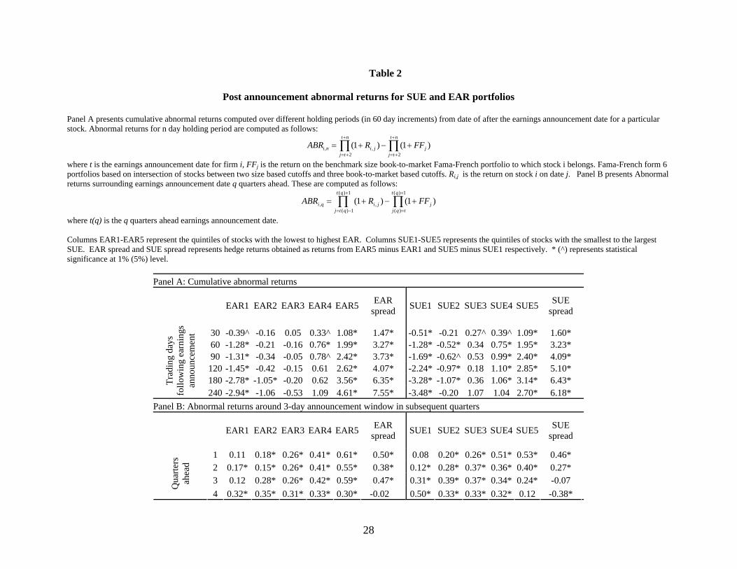
The results presented in Table 2 Panel A show that the cumulative abnormal return to the
highest quintile SUE portfolio is significantly positive over extended holding periods after the
earnings announcement. Similarly, the lowest quintile SUE portfolio earns significantly negative
cumulative abnormal returns. Thus, a long position in the high SUE stocks (quintile 5) and a
short position in the low SUE stocks (quintile 1) yields an average abnormal return of about
3.23% over the 60 trading days subsequent to the earnings announcement. The returns are much
higher (about 5.10%) when the equity positions are held for 120 trading days. After 180 trading
13
days, the SUE strategy becomes weak and shows signs of a reversal. These findings are
consistent with those reported by Bernard and Thomas (1989) and Jegadeesh and Livnat (2005).
Turning to the returns from EAR portfolios, a similar pattern is observed. For example,
firms in the highest (lowest) quintile of EAR stocks earn significant positive (negative) returns
over extended periods following the earnings announcement. A strategy of buying (selling) high
(low) EAR stocks results in an average abnormal return of 3.27% and 4.07% for the 60 and 120
day holding periods following the earnings announcement, respectively. However, there is no
return reversal after 180 trading days.
In the short run, it appears that both trading strategies generate comparable abnormal
returns on average, with the EAR strategy being slightly inferior. As we increase the holding
period, the SUE trading strategy generates 6.18% returns over 240 trading days following the
earnings announcement. For the same holding period, the EAR strategy earns 7.55%,
respectively. Therefore, over increasingly longer holding periods, the returns to both strategies
first appear to converge and then diverge. After one year following the earnings announcement,
the EAR strategy generates slightly higher abnormal returns on average than the SUE strategy.
While both strategies appear to produce similar abnormal returns on average, this does
not automatically imply that either of these strategies subsumes the other. An examination of
abnormal returns in the three day earnings announcement window in the subsequent 4 quarters
provides the first clue on the independent nature of the two strategies (see Table 2, Panel B).
Consistent with prior research, we find that a significant portion of the subsequent abnormal
returns to the SUE strategy occurs around earnings announcement dates. The three-day
announcement window stock returns surrounding subsequent quarterly earnings announcements
based on a strategy that takes a long position in extreme positive SUE stocks and a short position
14
in extreme negative SUE stocks generates 0.46%, 0.27%, -0.07% and -0.38% abnormal returns
in the four subsequent quarters, respectively. This indicates that part of the market reactions
around earnings announcements is predictable based on current period earnings surprises.
However, the predictive ability is monotonically declining over time and becomes less
significant, economically and statistically, in the four quarters subsequent to portfolio formation.
The return pattern observed for the EAR strategy, reported in Panel B of Table 2, is markedly
different. The 3 day window abnormal returns around subsequent earnings announcement dates
do not seem to monotonically decrease and reverse. The magnitude of EAR strategy (EAR5-
EAR1) abnormal returns around subsequent announcement dates remains almost stable and
becomes statistically insignificant by the fourth quarter. The EAR strategy generates one quarter
ahead and three quarter ahead 3-day announcement window abnormal returns equal to 0.5%,
0.38% and 0.47% respectively. Overall, the findings indicate that the two strategies based on
SUE and EAR are likely to be independent although they appear to generate similar cumulative
long run abnormal returns. Thus, market participants fail to reflect fully the information
contained in both earnings and non-earnings news conveyed at the time of earnings release.
4.2 Examination of a joint SUE and EAR strategy
The evidence in Table 2 suggests that EAR and SUE based abnormal returns are
potentially two independent phenomena, and it is plausible to expect each to not be subsumed by
the other. In this section, we examine to what extent these two strategies overlap with and differ
from each other. To accomplish this, we focus on the interactions of returns from the
independent sorts of EAR and SUE strategies. First, we conduct tests to assess whether the EAR
strategy is viable after holding SUE constant and vice versa. Such an analysis provides

15
information about how each of the strategies performs across different portfolios of the other (see
Reinganum 1981, Jaffe et al. 1989).
Table 3 presents the cumulative abnormal returns to each of the portfolios across several
holding periods in 30 trading day and 90 trading day increments. As before, we focus our
attention on 30, 60, 90, 120, 180, and 240 day holding periods. As is evident from the results
across all the holding periods, each strategy makes money independent of the other strategy.
That is, holding the SUE (EAR) quintile constant, the EAR (SUE) strategies make consistent
returns. For example, in the 60 day holding period the returns to the SUE strategy are 2.35%,
2.24%, 2.26%, 2.87%, and 4.79% across EAR quintiles 1 through 5. Similarly, the EAR
strategy generates returns of 1.53%, 2.17%, 2.30%, 3.40%, and 3.97%, respectively, across
quintiles 1 to 5 of SUE. As the holding periods increase to 180 and 240 trading days, the returns
to each of the strategies increase considerably, but what is noteworthy is that each of the
strategies performs consistently across all the quintiles of the other strategy.
To provide additional evidence on the independent nature of these two strategies we
conduct a nonoverlap hedge test as in Desai et al. (2005). The basic idea behind the nonoverlap
test is to assess the extent to which the EAR or the SUE strategy are able to generate returns after
eliminating convergent extreme groups, i.e., eliminating firms in the lowest EAR and SUE
portfolios (i.e., top left corner cell) and similarly firms in the highest EAR and SUE portfolios
(i.e., bottom right corner cell). That is, when examining the extreme quintiles of the independent
EAR strategy, we eliminate firms in the extreme quintile of the SUE strategy, and vice versa. In
this way, we can ensure that the two strategies are independent if they generate returns even after
eliminating firms that generate returns for the other strategy. Panel B of Table 3 presents the
findings of the nonoverlap hedge tests. Across all the holding periods, we find that both the
16
EAR and SUE strategies generate significant abnormal returns even after removing firms in the
extreme quintiles of the intersection of EAR and SUE portfolios. For example, for the 60 day
holding period, the EAR strategy earns a hedge return of 2.01%, whereas the SUE strategy earns
a hedge return of 2.1%. This demonstrates that the two strategies are largely independent.
Next, we consider whether we can exploit the two strategies to generate even greater
abnormal returns than can be obtained by each of the individual strategies alone. If the SUE and
EAR strategies are indeed distinct mispricing phenomena, then we should be able exploit both
elements of mispricing to create a combined strategy that would yield significantly higher
abnormal returns. Given that market participants appear to under-react to both earnings and non-
earnings information, ex ante we predict that by taking trading positions on the extreme cells in
the diagonal, i.e., firms in the extreme quintiles of both EAR and SUE (top left corner and
bottom right corner cells), we should earn larger abnormal returns than those obtained using the
individual strategies. Results presented in Table 3 are consistent with the prediction. For
example, in the 60 day holding period we can obtain a return of 6.32% by taking a long position
in the high SUE/high EAR portfolio (return of 4.12%) and a short position in the low SUE/low
EAR portfolio (return of -2.20%). This return is almost double that obtained for either strategy
on its own (see Table 2, Panel A).
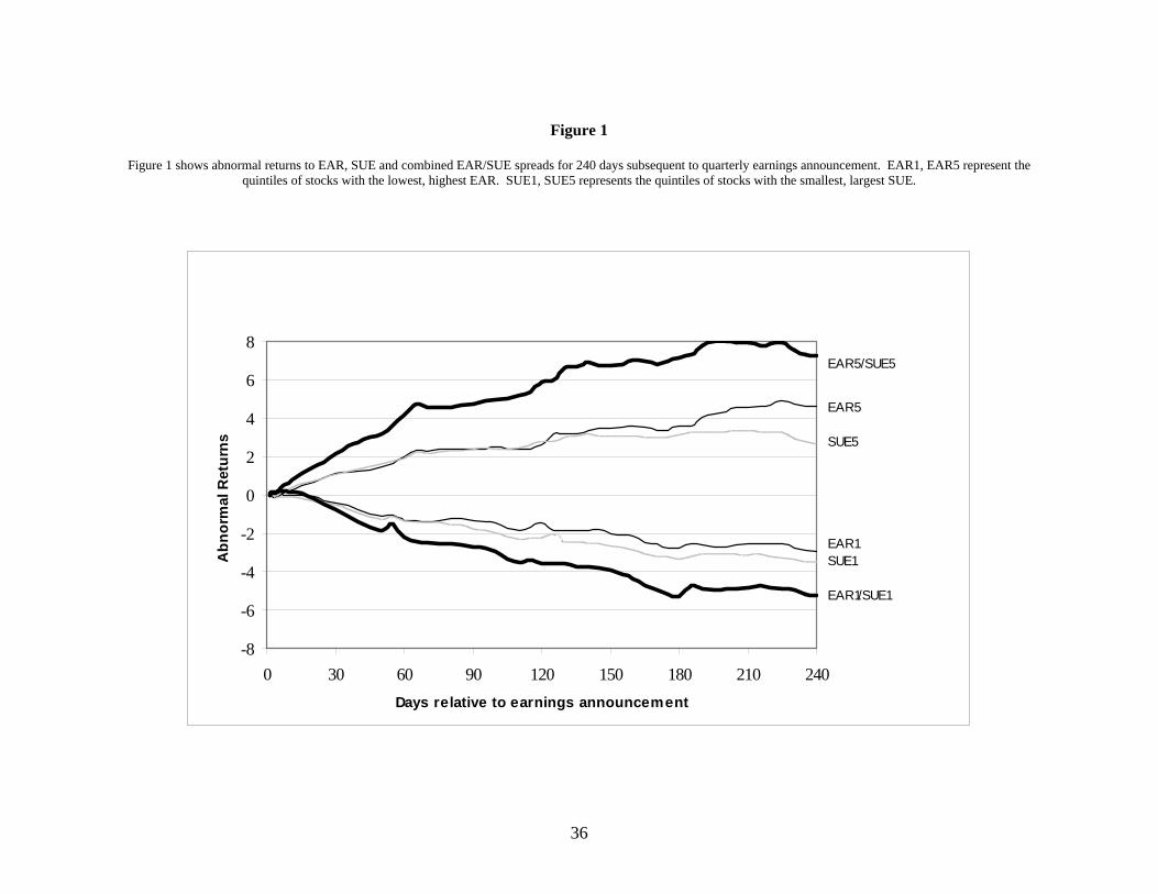
The returns obtained for the joint strategy are further illustrated in Figure 1, which plots
cumulative abnormal returns over 240 trading days starting with the day after the earnings
announcement. Six cumulative return series are plotted in this figure. First, we plot the return
pattern for extreme deciles of SUE (SUE1, SUE5) and EAR (EAR1, EAR5). Next, we plot the
returns for the joint strategies (EAR5/SUE5, EAR1/SUE1). Notice that the returns to the joint
high SUE/ high EAR portfolios are significantly higher than the returns earned on either the
17
highest SUE or EAR portfolios alone. Similarly, portfolios that contain firms with the lowest
SUE and the lowest announcement day stock returns experience significantly more negative
returns on average than those experienced by firms in the lowest SUE or the lowest EAR
quintiles separately. Thus, Figure 1 further highlights the superior returns obtained for the joint
SUE/EAR strategy.
We now consider two-by-two independent sorts of returns to EAR and SUE quintile
portfolios surrounding subsequent earnings announcements. The results, presented in Table 4,
provide further evidence on the independence of SUE and EAR. With the exception of the
SUE4 quintile for one and three-quarter ahead announcements, for any SUE quintile, returns to
the EAR strategy (i.e., EAR5 - EAR1) generates strong positive returns. Similarly, the SUE
strategy generates strong positive returns one quarter ahead, across all the EAR quintiles. The
return reversal pattern surrounding the fourth quarter subsequent to the portfolio formation is
present only for the SUE strategy across all the EAR quintiles with the exception of EAR4. The
return patterns are sufficiently different across quarters and different between the EAR and SUE
strategies, that we can conclude that the two strategies operate independent of each other.
4.3 EAR and SUE profitability through time
Table 5 examines the EAR and SUE strategies over two sub-samples, 1987 through 1995
and 1996 through 2004, to examine the time-series stability of the two anomalies. Panel A
reports the average abnormal returns over the three days surrounding the initial announcement
and Panel B reports the average abnormal three-day returns for the subsequent four
announcements. This sub-sample analysis highlights two striking differences between the two
strategies. Looking first at Panel A, we notice that the contemporaneous (i.e., perfect foresight)
return spread for the EAR sort increased from 16.47% to 21.68%, about a 30% rise from the first
18
to the second sub-sample. In contrast, the contemporaneous return spread for the SUE sort
decreased 3.62% to 3.25%, about a 10% relative drop. The increase in the contemporaneous
return spread for the EAR sort implies that stock prices have become more sensitive to the
information released in quarterly announcements (see Maydew and Landsman 2002). The
considerable drop in the contemporaneous return spread for the SUE sort implies further that this
increased sensitivity is not attributed to information about earnings. In fact, stock prices seem to
have become less sensitive to earnings-related information. This observation is consistent with
the findings of Lev and Zarowin (1999) and Ryan and Zarowin (2003).
Turning to Panel B of Table 5, we observe the same sub-sample pattern for the average
abnormal returns surrounding the next four earnings announcements. For example, the one-
quarter ahead average abnormal return from the EAR strategy increases by 13 basis points, from
0.44% in the 1987-1995 period to 0.57% in the 1996-2004 period. This is an increase upwards of
about 30%. The corresponding average abnormal returns from the SUE strategy, in contrast,
falls from 0,48% to 0.45%. Finally, it is interesting to note that the increase in the average
abnormal returns for the EAR strategy from the first sub-sample to the second is consistently
strong for three quarters subsequent to the earnings announcement. On the other hand, for SUE,
from the first sub-sample to the second, the magnitude of returns around subsequent earnings
announcement dates decreases for all four subsequent earnings announcement dates. In sum, the
EAR effect has grown stronger over the years whereas the SUE effect has weakened.
4.4. Robustness checks
4.4.1. EAR vs. price momentum
Sorting on announcement day returns is clearly related to sorting on past cumulative
returns, which is the basis of the price momentum anomaly documented by Chan et al (1996),
19
among others. It is therefore natural to examine how, if at all, and to what extent the EAR
anomaly is related to price momentum. Chan et al (1996) already shed some light on this issue,
by showing that price momentum is not driven entirely by past and future announcement day
returns. Their analysis does not reveal, however, whether the converse is also true – whether the
EAR anomaly is simply a restatement of price momentum.
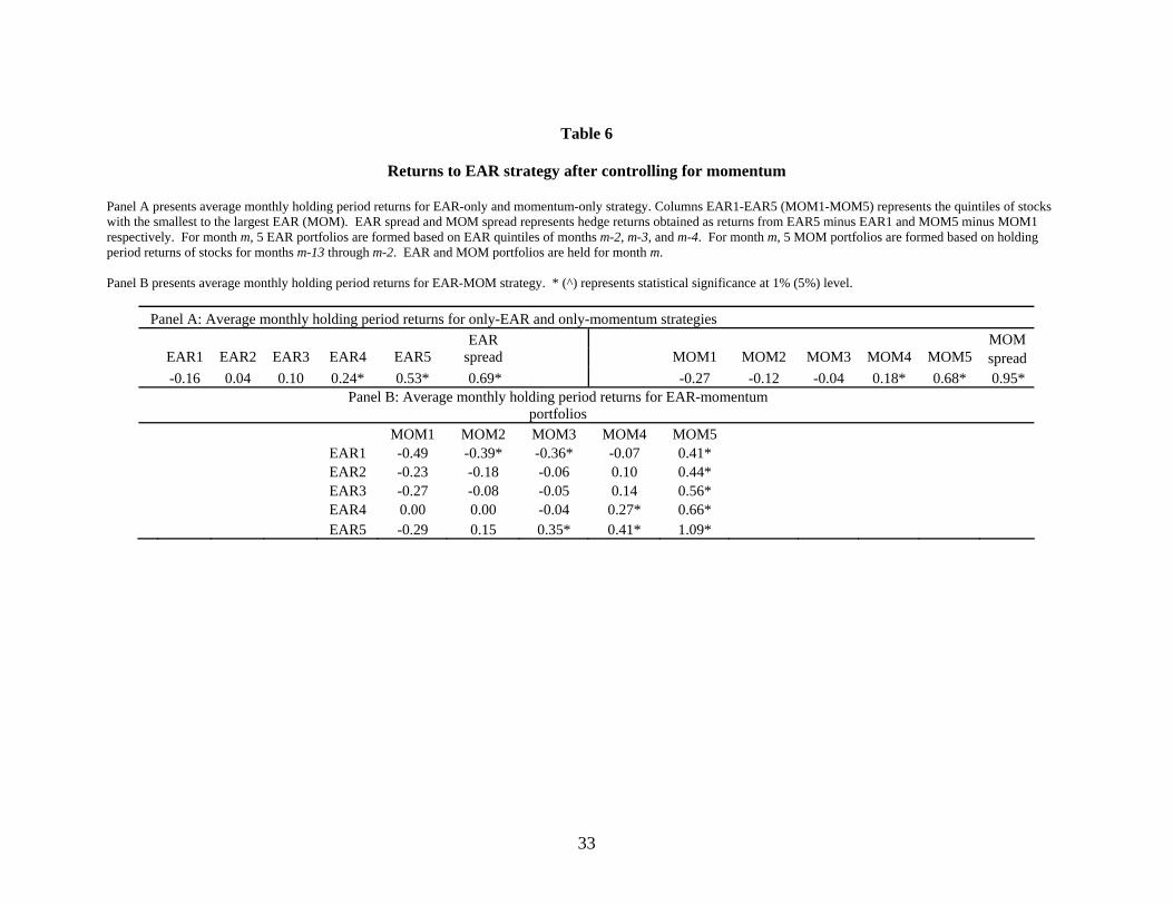
Table 6 shows that the EAR and the price momentum strategies are largely independent
of each other. Each month, stocks are given EAR and MOMENTUM ranks. For month m, five
EAR ranks (EAR1 through EAR5) are allocated based on quintiles of 3-day abnormal returns
around earnings announcements during months m-2 through m-4. Similarly, five MOMENTUM
ranks (MOM1 through MOM5) are given based on holding period returns for all stocks in the
CRSP universe from m-13 to m-2. We find that the EAR strategy produces abnormal returns
after controlling for MOMENTUM and vice-versa. Panel A shows the average monthly returns
using univariate sorts and Panel B presents results for bivariate sorts.
Panel A of the table shows that in the monthly implementation, the momentum sort
results in a significantly higher average hedge return – an annualized 11.4% versus 8.28% for the
EAR sort. Panel B of Table 2 shows an EAR strategy return of 7.55% for 240 trading days
(roughly equivalent to one year). This difference is, however, largely driven by the fact that we
impose on the EAR variable the standard monthly implementation of the momentum strategy.
Rather than hold all good- and bad-news positions through the subsequent four earnings
announcements, we resort the portfolio every month. From Figure 1, we see that the gradient for
the EAR strategy (or, the rate at which EAR return increases with time), is steepest for the first
60 trading days. Therefore, by rebalancing each month, the EAR portfolio captures the part of
the EAR return curve with steepest ascent. Of course, we could have alternatively imposed on

20
the momentum variable the future announcement day implementation of the EAR strategy (i.e.,
sort stocks in event time as opposed to calendar time and then hold them for four quarters), but
we already know from Chen et al (1996) that the returns to momentum are only partially related
to future announcement day returns. We therefore interpret our analysis in Table 6 as
conservatively stacking the deck in favor of the momentum sort.
Before we look at the returns from double sorting, we examine the composition of the
extreme EAR and Momentum portfolios in the single sort. In unreported results, we find that the
overlap is only marginally greater than that reported for the EAR and SUE portfolios. For
example, on average less than 35% of the stocks are common to the highest EAR and highest
momentum portfolios. This further suggests that the two anomalies are quite distinct.
Panel B presents the average monthly returns from independent double-sorting on the
EAR and the momentum variables. The EAR sort produces a 20 to 70 basis point spread in each
of the momentum quintiles. The momentum sort is also profitable in each of the EAR quintiles,
but especially so in the EAR5 quintile (firms with extremely good news in the last quarterly
announcement as measured through the announcement day returns) where it yields an average
annualized return of 16.6%. Again, the fact that the momentum strategy is profitable when
controlling for EAR is not surprising given the results of Chen et al (1996) and the fact that the
implementation favors momentum. The important observation is that the converse is also largely
true – the EAR strategy is profitable even when controlling for momentum. We therefore
conclude that the EAR anomaly is not a mere manifestation of the price momentum anomaly.
4.4.2. EAR and SUE for large firms
It is well known that small firms are more opaque than large ones (Imhoff 1992; Lang
and Lundholm 1993). Furthermore, the more opaque a firm’s operational and/or financial
21
condition is, the more should the firm’s stock price react to the quarterly release of information
by management (Collins, Kothari and Rayburn 1987). It may therefore be quite possible that the
extreme portfolios of the EAR sort contain predominantly small firms. This would raise
questions about the economic relevance of our result, since it is obviously difficult to exploit
small-firm anomalies in a meaningful scale. If the EAR anomaly is limited to small firms, it may
be explained by standard limits-to-arbitrage arguments.
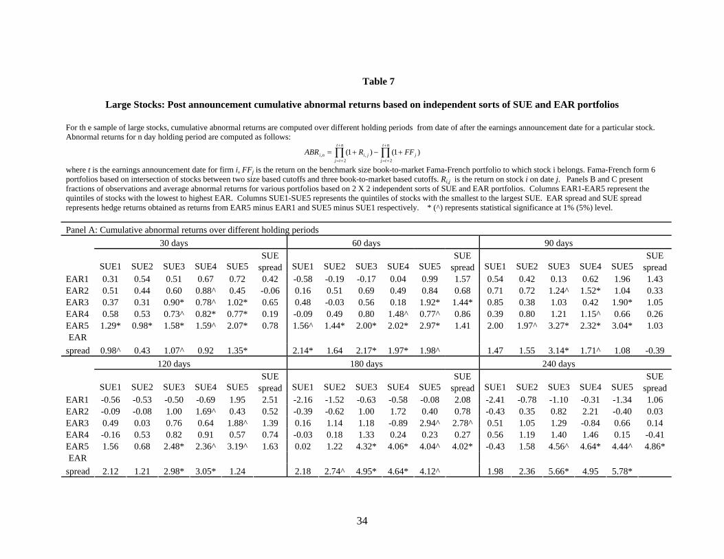
Table 7 duplicates our main Table 3 using only the top 1,000 largest firms in the CRSP
universe. There are two striking results that emerge from this table. First, it is clear that the
profitability of the EAR sort is considerably reduced, yet far from eliminated, in this large-cap
universe. For example, for holding periods of 30, 60, 90, 120, 180, and 240 trading days, EAR5-
EAR1 is statistically significant and positive for at least three SUE quintiles. For holding periods
of 120 and 90 trading days, EAR5-EAR1 is positive and statistically significant for two SUE
quintiles. While the reduction in the abnormal return is consistent with our argument about the
opacity of small firms, the EAR sort still produces economically meaningful abnormal returns in
the large-cap universe.
The second important result is that the SUE sort is much more sensitive to the elimination
of small firms than the EAR sort. In particular, in most of the cases (different horizons and EAR
quintiles) the SUE spread return is statistically insignificant. This shows clearly that a
significant portion of the abnormal returns of the SUE strategy is attributable to mispricing of
small firms (Bernard and Thomas 1990).
4.4.3. EAR and SUE with analyst forecasts
Are insignificant SUE strategy abnormal returns the result of a misspecified model of
expected earnings? It could be that a seasonal random walk with drift model of earnings

22
expectations is not what the market actually uses on an aggregate basis and hence the SUE
measure constructed for the analysis above may be unable to capture the true earnings surprises
perceived by investors. Consistent with this argument, Livnat and Mendenhall (2006) and
Battalio and Mendenhall (2005) document that the post earnings announcement drift is
significantly larger when defining earnings surprise based on analyst forecasts rather than a time-
series expectation model. Therefore, we ascertain the sensitivity of our findings by using IBES
consensus analyst forecasts as an alternative measure of earnings expectations.
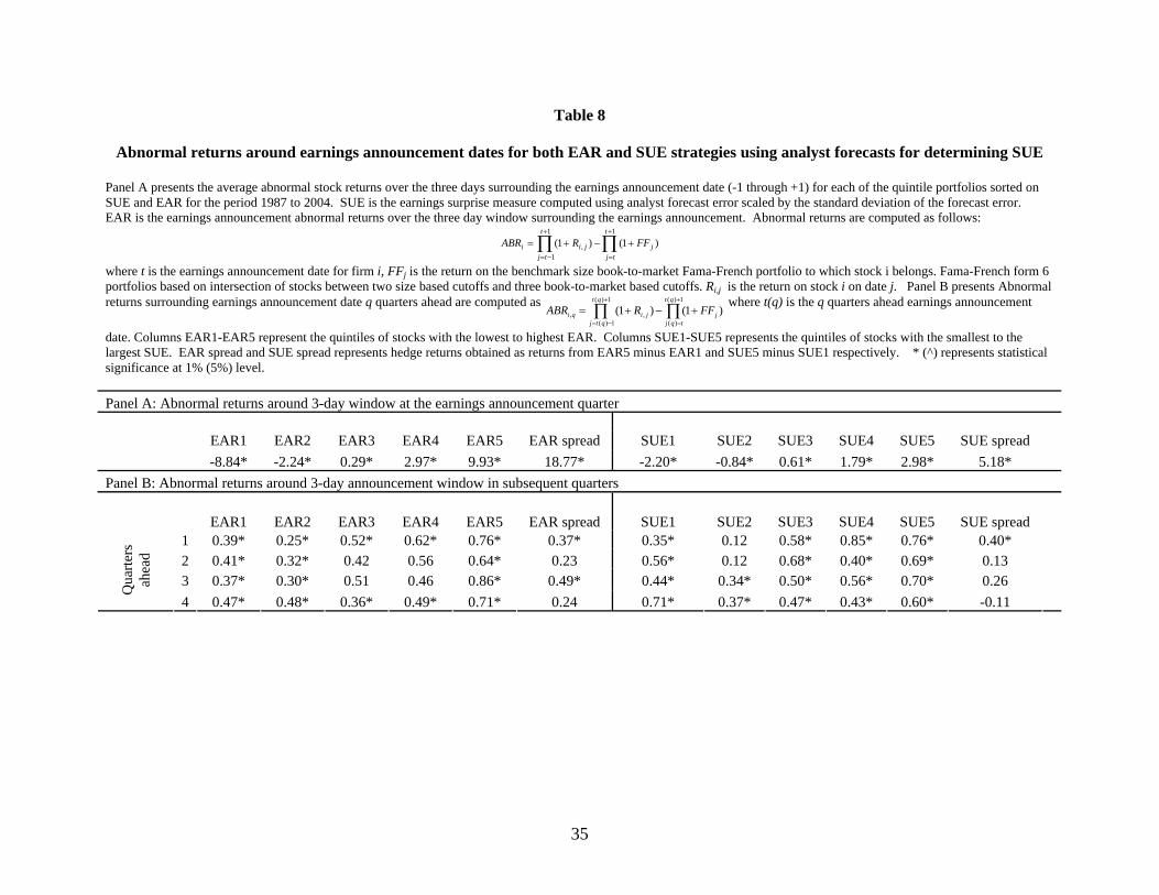
Panel A of Table 8 shows the three-day announcement window returns of EAR and SUE
sorted portfolio with SUE now calculated using IBES mean consensus estimates for expected
earnings. This panel is directly comparable to Panel A of Table 1, except the sample is smaller
due to limited IBES coverage. Comparing the SUE spread return of 5.18% to the corresponding
value of 3.41% from Table 1, suggests that a better measure of earnings surprise using IBES
forecasts helps in a significant improvement in announcement day returns. The results do
confirm the findings of Doyle, Lundholm and Soliman (2005) that using IBES forecasts instead
of a seasonal random walk with drift model for expected earnings improves considerably the
performance of the SUE strategy (see also Livnat and Mendenhall (2006)). However, the return
difference is not significantly different for the EAR sort (18.77% in Table 8 vs 19.13% in Table
3) indicating that the reduced sample size due to the IBES coverage can not explain the improved
returns for the SUE sort.
Panel B of Table 8 reports the abnormal returns of the EAR and SUE sorted portfolios
around the subsequent four earnings announcements, analogous to Panel B of Table 2.
Qualitatively, the results for abnormal returns around subsequent announcement dates using
analyst forecasts remain the same as compared to the results using seasonally random walk with
23
drift. In terms of statistical significance, however, only the strategy for the first subsequent
quarter demonstrates statistically significant returns. For the IBES sample, we see statistically
significant EAR strategy returns for the first and third quarter subsequent to the earnings
announcement. Overall, Table 8 confirms that the EAR measure captures something more
fundamental than mismeasurement of the market’s earnings forecasts.
5. Conclusion
We unearth a new dimension to the post earnings announcement drift anomaly. We
document that, in addition to under reacting to the earnings surprise revealed at the time of
earnings release, the market seems to under react to other information contained in the
announcement. Consistent with existing literature, we find that the portion of the announcement
date abnormal returns attributable to the earnings surprise is dwarfed by the other relevant
information in the announcement. In particular, for at least 40% of stocks with positive
(negative) earnings surprises, investors earn negative (positive) abnormal returns around
earnings announcements.
Return patterns observed for the SUE and EAR strategies are different in many respects.
First, we find that a long-short strategy based on an EAR sort generates significant abnormal
returns over one year horizon. These returns are larger than the returns of the SUE strategy.
These abnormal returns obtain even after controlling for the SUE strategy. Second, the
announcement window EAR returns for subsequent quarters do not seem to decline
monotonically. They remain significant up to the third quarter following portfolio formation.
Furthermore, unlike the return reversal in the 4th quarter for SUE strategy, we do not find any
reversal for the EAR strategy. Third, while the returns to the SUE strategy appear to have waned
24
over the years, the returns to the EAR strategy have, in fact, increased over time. Finally, for
large stocks, the post earnings announcement drift for the EAR effect is much stronger than for
the SUE effect.
The abnormal returns obtained for the EAR strategy are robust to several additional
sensitivity tests. The EAR strategy is neither subsumed by nor subsumes the price momentum
strategy. It is also robust to restricting the universe of stocks to large caps only. Using analyst
forecasts for earnings expectations does not change our results in any way.
Our findings are intriguing in that we are able to generate predictable abnormal returns
using a conspicuous piece of information, the earnings announcement returns. They indicate a
systematic under reaction to both earnings and non-earnings information that is disseminated
around earnings announcements. This adds a new dimension to the long-standing post-earnings
announcement drift anomaly.

25
References
Ball, R., and E. Bartov. 1996. How Naive is the Stock Market's Use of Earnings Information?, Journal of Accounting and Economics 21: 319-337.
Ball, R., and P. Brown. 1968. An Empirical Evaluation of Accounting Numbers, Journal of
Accounting Research 6: 159-178. Battalio, R.H., and R. R. Mendenhall, 2005. Earnings expectations, investor trade size, and
anomalous returns around earnings announcements, Journal of Financial Economics 77: 289-319.
Bernard, V. L., and J. Thomas. 1989. Post-Earnings Announcement Drift: Delayed Price
Response or Risk Premium, Journal of Accounting Research 27: 1-35. Chan, L. K.C., N. Jegadeesh, and J. Lakonishok. 1996 Momentum Strategies, Journal of
Finance 51: 1681–1713. Chordia, Tarun, and L. Shivakumar. Earnings and Price Momentum, forthcoming Journal of
Financial Economics. Doyle, J.T., R.J. Lundholm, and M.T. Soliman. 2005. The Extreme Future Stock Returns
Following Extreme Earnings Surprises. Working Paper, Stanford University. Fama, E. 1998. Market Efficiency, Long-term Returns and Behavioral Finance, Journal of
Financial Economics 49: 283-306. Fama, E., and K. R. French. 1992. The Cross-section of Expected Stock Returns, Journal of
Finance 47: 427-465. Fama, E., and K. R. French. 1993. Common Risk Factors in the Returns on Stocks and Bonds,
Journal of Financial Economics 33: 3-56. Fama, E., and K. R. French. 1996. Multifactor Explanations of Asset Pricing Anomalies, Journal
of Finance 51: 55–84. Foster, G., C. Olsen, and T. Shevlin. 1984. Earnings Releases, Anomalies, and the Behavior of
Security Returns, The Accounting Review: 574-603. Francis, J., K. Schipper, and L. Vincent. 2002. Expanded Disclosures and the Increased
Usefulness of Earnings Announcements, The Accounting Review 77: 515-546. Gu. 2005. Innovation, Future Earnings, and Market Efficiency, Journal of Accounting, Auditing
& Finance 20: 385-418.

26
Hutton 2005. Determinants of Managerial Earnings Guidance Prior to Regulation Fair Disclosure and Bias in Analysts’ Earnings Forecasts, Contemporary Accounting Research 22:867-914.
Imhoff, E.A. 1992. The Relation between Perceived Accounting Quality and Economic
Characteristics of the Firm, Journal of Accounting and Public Policy 11: 97-118. Jegadeesh, N. 1990. Evidence of Predictable Behavior in Security Returns, Journal of Finance
45: 881-898. Jegadeesh, N., and J. Livnat. 2004. Revenue Surprises and Stock Returns, Working Paper. Jegadeesh, N., and S. Titman. 1993. Returns to Buying Winners and Selling Losers: Implications
for Stock Market Efficiency, Journal of Finance 48: 65–91. Jegadeesh, N., and S. Titman. 2001. Profitability of Momentum Strategies: An Evaluation of
Alternative Explanations, Journal of Finance 56: 699-720. Lang, M., and R. Lundholm. 1993. Cross-sectional Determinants of Analyst Ratings of
Corporate Disclosures, Journal of Accounting Research 31: 246-271. Lev, B. 1989. On the Usefulness of Earnings and Earnings Research: Lessons and Directions
from Two Decades of Empirical Research, Journal of Accounting Research 27: 153-192 Lev, B., and P. Zarowin. 1999. The Boundaries of Financial Reporting and How to extend
them, Journal of Accounting Research 37: 353-385. Liu, J., and Thomas, J. 2000. Stock Returns and Accounting Earnings, Journal of Accounting
Research 38: 71-101 Livnat, J., and R.R. Mendenhall. 2006. Comparing the Post-Earnings Announcement Drift for
Surprises Calculated from Analyst and Time-Series Forecasts, Journal of Accounting Research 44: 177-204.
Maydew, E.L., and W.R. Landsman. 2002. Has the information content of quarterly earnings
announcements declined in the past three decades?, Journal of Accounting Research 40: 797-808.
Rajgopal, S., T. Shevlin, and M. Venkatachalam. 2003. Does the Stock Market Fully Appreciate
the Implications of Leading Indicators for Future Earnings? Evidence from Order Backlog, Review of Accounting Studies 8: 461-492.
Ryan, S., and P. Zarowin. 2003. Why Has the Contemporaneous Linear Returns-Earnings
Relation Declined?, Journal of Accounting Research 78: 523-553.

27
Table 1
Abnormal returns around earnings announcement dates
Panel A presents the average abnormal stock returns over the three days surrounding the earnings announcement date (-1 through +1) for each of the quintile portfolios sorted on SUE and EAR for the period 1987 to 2004. SUE is the earnings surprise measure computed as the seasonally differenced quarterly earnings scaled by the standard deviation of the forecast error. EAR is the earnings announcement abnormal returns over the three day window surrounding the earnings announcement. Abnormal returns are computed as follows:
)1()1(1
1
1
,∏ ∏+
−=
+
=
+−+=t
tj
t
tjjjii FFRABR
where t is the earnings announcement date for firm i, FFj is the return on the benchmark size book-to-market Fama-French portfolio to which stock i belongs. Fama-French form 6 portfolios based on intersection of stocks between two size based cutoffs and three book-to-market based cutoffs. Ri,j is the return on stock i on date j. Panels B and C present fractions of observations and average abnormal returns for various portfolios based on 2 X 2 independent sorts of SUE and EAR portfolios. Columns EAR1-EAR5 represent the quintiles of stocks with the lowest to highest EAR. Columns SUE1-SUE5 represent the quintiles of stocks with the smallest to the largest SUE. EAR spread and SUE spread represents hedge returns obtained as EAR5 – EAR1 and SUE5 – SUE1 respectively. * (^) represents statistical significance at 1% (5%) level.
Panel A: Abnormal returns around 3-day announcement window SUE
EAR1 EAR2 EAR3 EAR4 EAR5 EAR spread SUE1 SUE2 SUE3 SUE4 SUE5
spread -8.99* -2.38* 0.10* 2.74* 10.14* 19.13* -1.40* -0.40* 0.30* 1.09* 2.01* 3.41*
Panel B: Fraction of firms in each quintile Panel C: Abnormal returns around 3-day announcement window SUE spread
SUE1 SUE2 SUE3 SUE4 SUE5 SUE1 SUE2 SUE3 SUE4 SUE5 (SUE5 – SUE1)
EAR1 0.28 0.22 0.19 0.16 0.15 EAR1 -9.78* -8.88* -8.60* -8.64* -8.53* 1.24* EAR2 0.22 0.22 0.20 0.19 0.17 EAR2 -2.41* -2.38* -2.38* -2.36* -2.36* 0.05* EAR3 0.19 0.21 0.21 0.20 0.19 EAR3 0.08^ 0.09^ 0.09* 0.11* 0.12* 0.04* EAR4 0.17 0.19 0.20 0.21 0.23 EAR4 2.69* 2.73* 2.74* 2.76* 2.79* 0.10*
EAR
Qui
ntile
s
EAR5 0.14 0.16 0.19 0.23 0.28 EAR5 9.75* 9.65* 9.66* 10.14* 10.92* 1.17*
EAR Spread (EAR5 – EAR1)
19.53* 18.53* 18.26* 18.77* 19.46*
28
Table 2
Post announcement abnormal returns for SUE and EAR portfolios
Panel A presents cumulative abnormal returns computed over different holding periods (in 60 day increments) from date of after the earnings announcement date for a particular stock. Abnormal returns for n day holding period are computed as follows:
)1()1(2 2
,, ∏ ∏+
+=
+
+=
+−+=nt
tj
nt
tjjjini FFRABR
where t is the earnings announcement date for firm i, FFj is the return on the benchmark size book-to-market Fama-French portfolio to which stock i belongs. Fama-French form 6 portfolios based on intersection of stocks between two size based cutoffs and three book-to-market based cutoffs. Ri,j is the return on stock i on date j. Panel B presents Abnormal returns surrounding earnings announcement date q quarters ahead. These are computed as follows:
)1()1(1)(
1)(
1)(
)(,, ∏ ∏
+
−=
+
=
+−+=qt
qtj
qt
tqjjjiqi FFRABR
where t(q) is the q quarters ahead earnings announcement date. Columns EAR1-EAR5 represent the quintiles of stocks with the lowest to highest EAR. Columns SUE1-SUE5 represents the quintiles of stocks with the smallest to the largest SUE. EAR spread and SUE spread represents hedge returns obtained as returns from EAR5 minus EAR1 and SUE5 minus SUE1 respectively. * (^) represents statistical significance at 1% (5%) level.
Panel A: Cumulative abnormal returns
EAR1 EAR2 EAR3 EAR4 EAR5 EAR
spread SUE1 SUE2 SUE3 SUE4 SUE5 SUE spread
30 -0.39^ -0.16 0.05 0.33^ 1.08* 1.47* -0.51* -0.21 0.27^ 0.39^ 1.09* 1.60* 60 -1.28* -0.21 -0.16 0.76* 1.99* 3.27* -1.28* -0.52* 0.34 0.75* 1.95* 3.23* 90 -1.31* -0.34 -0.05 0.78^ 2.42* 3.73* -1.69* -0.62^ 0.53 0.99* 2.40* 4.09*
120 -1.45* -0.42 -0.15 0.61 2.62* 4.07* -2.24* -0.97* 0.18 1.10* 2.85* 5.10* 180 -2.78* -1.05* -0.20 0.62 3.56* 6.35* -3.28* -1.07* 0.36 1.06* 3.14* 6.43* Tr
adin
g da
ys
follo
win
g ea
rnin
gs
anno
unce
men
t
240 -2.94* -1.06 -0.53 1.09 4.61* 7.55* -3.48* -0.20 1.07 1.04 2.70* 6.18* Panel B: Abnormal returns around 3-day announcement window in subsequent quarters
EAR1 EAR2 EAR3 EAR4 EAR5 EAR
spread SUE1 SUE2 SUE3 SUE4 SUE5 SUE spread
1 0.11 0.18* 0.26* 0.41* 0.61* 0.50* 0.08 0.20* 0.26* 0.51* 0.53* 0.46* 2 0.17* 0.15* 0.26* 0.41* 0.55* 0.38* 0.12* 0.28* 0.37* 0.36* 0.40* 0.27* 3 0.12 0.28* 0.26* 0.42* 0.59* 0.47* 0.31* 0.39* 0.37* 0.34* 0.24* -0.07
Qua
rters
ah
ead
4 0.32* 0.35* 0.31* 0.33* 0.30* -0.02 0.50* 0.33* 0.33* 0.32* 0.12 -0.38*

29
Table 3
Post announcement cumulative abnormal returns based on independent sorts of SUE and EAR portfolios
Cumulative abnormal returns are computed over different holding periods from date of after the earnings announcement date for a particular stock. Abnormal returns for n day holding period are computed as follows:
)1()1(2 2
,, ∏ ∏+
+=
+
+=
+−+=nt
tj
nt
tjjjini FFRABR
where t is the earnings announcement date for firm i, FFj is the return on the benchmark size book-to-market Fama-French portfolio to which stock i belongs. Fama-French form 6 portfolios based on intersection of stocks between two size based cutoffs and three book-to-market based cutoffs. Ri,j is the return on stock i on date j. Panels B and C present fractions of observations and average abnormal returns for various portfolios based on 2 X 2 independent sorts of SUE and EAR portfolios. Columns EAR1-EAR5 represent the quintiles of stocks with the lowest to highest EAR. Columns SUE1-SUE5 represents the quintiles of stocks with the smallest to the largest SUE. EAR spread and SUE spread represents hedge returns obtained as returns from EAR5 minus EAR1 and SUE5 minus SUE1 respectively. * (^) represents statistical significance at 1% (5%) level.
Panel A: Cumulative abnormal returns over different holding periods 30 days 60 days 90 days
SUE SUE SUE SUE1 SUE2 SUE3 SUE4 SUE5spread
SUE1 SUE2 SUE3 SUE4 SUE5 spread
SUE1 SUE2 SUE3 SUE4 SUE5spread
EAR1 -0.75* -0.50* -0.05 -0.19 -0.05 0.70 -2.20* -1.56* -0.57 -1.28* 0.15 2.35* -2.68* -1.79* -0.55 -0.57 0.41 3.09*EAR2 -0.83* -0.25 -0.02 0.03 0.46* 1.29* -1.42* -0.46 0.09 0.12 0.81 2.24* -1.71* -0.81* 0.49 -0.24 1.11* 2.83*EAR3 -0.46* -0.40 0.08 0.15 0.90* 1.36* -0.98 -1.02 0.00 0.39 1.28* 2.26* -1.53* -0.89* 0.07 0.56 1.72* 3.26*EAR4 -0.40 -0.17 0.20 0.62* 1.18* 1.57* -0.94* -0.03* 0.28 1.66* 1.94* 2.87* -1.13* -0.16 0.29 1.95* 2.40* 3.53*EAR5 0.01 0.14 1.02* 1.07* 2.16* 2.15* -0.67 0.62 1.72* 2.14* 4.12* 4.79* -0.86 0.76 2.39* 2.71* 4.76* 5.62*
EAR spread 0.76^ 0.64^ 1.06* 1.26* 2.21* 1.53* 2.17* 2.30* 3.40* 3.97* 1.82* 2.54* 2.95* 3.28* 4.35*
120 days 180 days 240 days SUE SUE SUE
SUE1 SUE2 SUE3 SUE4 SUE5spread
SUE1 SUE2 SUE3 SUE4 SUE5 spread
SUE1 SUE2 SUE3 SUE4 SUE5spread
EAR1 -3.60* -2.24* -1.01 -0.81 1.22 4.82* -5.28* -3.11* -1.55 -1.17 -0.83 4.45* -5.24* -1.40 -2.35* -1.51 -1.77 3.47*EAR2 -2.01* -0.82 0.13 0.25 0.98 2.99* -2.90* -1.78* 0.04 -0.99 1.32 4.22* -3.25* -1.77* 1.03 -1.30 0.49 3.74*EAR3 -2.13* -1.18* -0.01 0.86 1.93* 4.06* -2.68* -0.85 -0.31 0.85 2.39* 5.07* -3.36* -0.72 0.17 0.04 1.74* 5.10*EAR4 -1.78* -0.35 0.21 1.83* 2.39* 4.17* -2.55* -0.50 0.61 1.67* 3.04* 5.59* -2.60* 0.59 0.80 2.87* 2.87* 5.47*EAR5 -0.96 0.25 1.87* 2.90* 5.84* 6.80* -1.63 1.35 3.14* 4.15* 7.15* 8.79* -1.87 3.02* 6.05* 4.66* 7.24* 9.11*
EAR spread 2.64* 2.49* 2.88* 3.71* 4.62* 3.65* 4.46* 4.69* 5.31* 7.99* 3.37* 4.42* 8.39* 6.17* 9.01*

30
Table 3 Continued
Panel B: Hedge returns over different holding periods after eliminating portfolios in the (SUE1,EAR1) and (SUE5, EAR5) cells
EAR spread SUE spread 30 0.92* 1.14* 60 2.01* 2.10* 90 2.29* 2.86*
120 1.98* 3.47* 180 4.01* 4.10* Tr
adin
g da
ys
follo
win
g ea
rnin
gs
anno
unce
men
t
240 5.50* 3.80*

31
Table 4
Abnormal returns around subsequent quarterly earnings announcements based on independent sorts of SUE and EAR portfolios Abnormal returns surrounding earnings announcement date q quarters ahead are computed as follows:
)1()1(1)(
1)(
1)(
)(,, ∏ ∏
+
−=
+
=
+−+=qt
qtj
qt
tqjjjiqi FFRABR
where t(q) is the q quarters ahead earnings announcement date, FFj is the return on the benchmark size book-to-market Fama-French portfolio to which stock i belongs. Fama-French form 6 portfolios based on intersection of stocks between two size based cutoffs and three book-to-market based cutoffs. Ri,j is the return on stock i on date j. Quintile portfolios sorted on SUE and EAR for the period 1987 to 2004 are formed based on SUE and EAR in the current quarter. SUE is the earnings surprise measure computed as the seasonally differenced quarterly earnings scaled by the standard deviation of the forecast error. EAR is the earnings announcement abnormal returns over the three day window surrounding the earnings announcement. * (^) represents statistical significance at 1% (5%) level. 1 quarter ahead 2 quarters ahead
SUE SUE SUE1 SUE2 SUE3 SUE4 SUE5 spread
SUE1 SUE2 SUE3 SUE4 SUE5 spread
EAR1 -0.09 -0.08 0.06 0.46* 0.42* 0.51 * -0.01 0.22* 0.32* 0.11 0.23 0.25 EAR2 0.07 0.06 0.24* 0.18 0.38* 0.31^ 0.08 0.10 0.31^ 0.08 0.22 0.14 EAR3 0.01 0.23* 0.20^ 0.43* 0.38* 0.36^ 0.17 0.22^ 0.35^ 0.30* 0.29* 0.12 EAR4 0.19 0.41* 0.24* 0.67* 0.46* 0.28^ 0.24* 0.46* 0.45* 0.44* 0.39* 0.15 EAR5 0.24 0.41* 0.57* 0.73* 0.84* 0.61* 0.19 0.48* 0.47* 0.68* 0.65* 0.46*
EAR spread 0.33^ 0.50* 0.50* 0.28 0.44^ 0.21 0.25 0.17 0.55* 0.40^
3 quarters ahead 4 quarters ahead SUE SUE
SUE1 SUE2 SUE3 SUE4 SUE5 spread
SUE1 SUE2 SUE3 SUE4 SUE5 spread
EAR1 0.14 0.05 0.11 0.15 0.05 -0.11 0.49* 0.19 0.38* 0.31 0.04 -0.45* EAR2 0.25* 0.38* 0.32* 0.22 0.26^ 0.02 0.61* 0.32* 0.32* 0.29^ 0.11 -0.51* EAR3 0.32* 0.33* 0.33* 0.15 0.10 -0.21 0.59* 0.26^ 0.32^ 0.24* 0.16 -0.43* EAR4 0.46* 0.53* 0.46* 0.53* 0.06 -0.40* 0.32* 0.44* 0.22* 0.41* 0.25* -0.07 EAR5 0.59* 0.73* 0.71* 0.59* 0.50* -0.06 0.45* 0.54* 0.35* 0.29* 0.08 -0.36^
EAR spread 0.41^ 0.71* 0.58* 0.43^ 0.47^ -0.05 0.35 -0.04 -0.02 0.04

32
Table 5
Abnormal returns around earnings announcement dates for both EAR and SUE strategies across two sub-periods (1987-1995:1996-2004)
Panel A presents the average abnormal stock returns over the three days surrounding the earnings announcement date (-1 through +1) for each of the quintile portfolios sorted on SUE and EAR for two subperiods between 1987 and 2004. SUE is the earnings surprise measure computed using analyst forecast error scaled by the standard deviation of the forecast error. EAR is the earnings announcement abnormal returns over the three day window surrounding the earnings announcement. Abnormal returns are computed as follows: )1()1(
1
1
1
,∏ ∏+
−=
+
=
+−+=t
tj
t
tjjjii FFRABR where t is the earnings announcement date for firm i, FFj is the return on the benchmark size book-to-market Fama-French portfolio to
which stock i belongs. Fama-French form 6 portfolios based on intersection of stocks between two size based cutoffs and three book-to-market based cutoffs. Ri,j is the return on stock i on date j. Panel B presents Abnormal returns surrounding earnings announcement date q quarters ahead are computed as
)1()1(1)(
1)(
1)(
)(,, ∏ ∏
+
−=
+
=
+−+=qt
qtj
qt
tqjjjiqi FFRABR
where t(q) is
the q quarters ahead earnings announcement date. Columns EAR1-EAR5 represent the quintiles of stocks with the lowest to highest EAR. Columns SUE1-SUE5 represents the quintiles of stocks with the smallest to the largest SUE. EAR spread and SUE spread represents hedge returns obtained as returns from EAR5 minus EAR1 and SUE5 minus SUE1 respectively. * (^) represents statistical significance at 1% (5%) level. Panel A: Abnormal returns around 3-day window at the earnings announcement quarter
SUE Sub period
EAR1 EAR2 EAR3 EAR4 EAR5 EAR spread SUE1 SUE2 SUE3 SUE4 SUE5
spread 1987-1995 -7.76* -2.18* -0.01 2.30* 8.71* 16.47* -1.58* -0.57* 0.17 1.02* 2.04* 3.62* 1996-2004 -10.10* -2.52* 0.23* 3.19* 11.58* 21.68* -1.21* -0.26* 0.43 1.22* 2.04* 3.25* Panel B: Abnormal returns around 3-day announcement window in subsequent quarters
Sub SUE period
Quarters ahead EAR1 EAR2 EAR3 EAR4 EAR5 EAR spread SUE1 SUE2 SUE3 SUE4 SUE5
spread 1 -0.02 0.01 0.23* 0.31* 0.42* 0.44* -0.06 0.04 0.14* 0.44* 0.42* 0.48* 2 0.10 0.08 0.15* 0.24* 0.39* 0.29* 0.01 0.08 0.25* 0.23* 0.35* 0.34* 3 -0.01 0.18* 0.14* 0.31* 0.50* 0.51* 0.28* 0.22* 0.24* 0.23* 0.13* -0.15
1987
-199
5
4 0.25* 0.25* 0.23* 0.21* 0.13* -0.13 0.43* 0.17* 0.31* 0.17* -0.03 -0.46* 1 0.25 0.36* 0.29* 0.51* 0.81* 0.57* 0.22* 0.35 0.40* 0.58* 0.67* 0.45* 2 0.25* 0.24* 0.37* 0.59* 0.73* 0.48* 0.26* 0.48* 0.51 0.49* 0.47* 0.21* 3 0.27 0.39* 0.40* 0.54* 0.69* 0.42* 0.34* 0.56* 0.52* 0.47* 0.36* 0.02
1996
-200
4
4 0.40* 0.47* 0.39* 0.47* 0.48* 0.08 0.59* 0.49 0.35* 0.48* 0.29* -0.30*
33
Table 6
Returns to EAR strategy after controlling for momentum
Panel A presents average monthly holding period returns for EAR-only and momentum-only strategy. Columns EAR1-EAR5 (MOM1-MOM5) represents the quintiles of stocks with the smallest to the largest EAR (MOM). EAR spread and MOM spread represents hedge returns obtained as returns from EAR5 minus EAR1 and MOM5 minus MOM1 respectively. For month m, 5 EAR portfolios are formed based on EAR quintiles of months m-2, m-3, and m-4. For month m, 5 MOM portfolios are formed based on holding period returns of stocks for months m-13 through m-2. EAR and MOM portfolios are held for month m. Panel B presents average monthly holding period returns for EAR-MOM strategy. * (^) represents statistical significance at 1% (5%) level.
Panel A: Average monthly holding period returns for only-EAR and only-momentum strategies MOM
EAR1 EAR2 EAR3 EAR4 EAR5 EAR
spread MOM1 MOM2 MOM3 MOM4 MOM5 spread -0.16 0.04 0.10 0.24* 0.53* 0.69* -0.27 -0.12 -0.04 0.18* 0.68* 0.95*
Panel B: Average monthly holding period returns for EAR-momentum
portfolios MOM1 MOM2 MOM3 MOM4 MOM5 EAR1 -0.49 -0.39* -0.36* -0.07 0.41* EAR2 -0.23 -0.18 -0.06 0.10 0.44* EAR3 -0.27 -0.08 -0.05 0.14 0.56* EAR4 0.00 0.00 -0.04 0.27* 0.66* EAR5 -0.29 0.15 0.35* 0.41* 1.09*
34
Table 7
Large Stocks: Post announcement cumulative abnormal returns based on independent sorts of SUE and EAR portfolios For th e sample of large stocks, cumulative abnormal returns are computed over different holding periods from date of after the earnings announcement date for a particular stock. Abnormal returns for n day holding period are computed as follows:
)1()1(2 2
,, ∏ ∏+
+=
+
+=
+−+=nt
tj
nt
tjjjini FFRABR
where t is the earnings announcement date for firm i, FFj is the return on the benchmark size book-to-market Fama-French portfolio to which stock i belongs. Fama-French form 6 portfolios based on intersection of stocks between two size based cutoffs and three book-to-market based cutoffs. Ri,j is the return on stock i on date j. Panels B and C present fractions of observations and average abnormal returns for various portfolios based on 2 X 2 independent sorts of SUE and EAR portfolios. Columns EAR1-EAR5 represent the quintiles of stocks with the lowest to highest EAR. Columns SUE1-SUE5 represents the quintiles of stocks with the smallest to the largest SUE. EAR spread and SUE spread represents hedge returns obtained as returns from EAR5 minus EAR1 and SUE5 minus SUE1 respectively. * (^) represents statistical significance at 1% (5%) level. Panel A: Cumulative abnormal returns over different holding periods
30 days 60 days 90 days SUE SUE SUE
SUE1 SUE2 SUE3 SUE4 SUE5 spread SUE1 SUE2 SUE3 SUE4 SUE5 spread SUE1 SUE2 SUE3 SUE4 SUE5 spread EAR1 0.31 0.54 0.51 0.67 0.72 0.42 -0.58 -0.19 -0.17 0.04 0.99 1.57 0.54 0.42 0.13 0.62 1.96 1.43 EAR2 0.51 0.44 0.60 0.88^ 0.45 -0.06 0.16 0.51 0.69 0.49 0.84 0.68 0.71 0.72 1.24^ 1.52* 1.04 0.33 EAR3 0.37 0.31 0.90* 0.78^ 1.02* 0.65 0.48 -0.03 0.56 0.18 1.92* 1.44* 0.85 0.38 1.03 0.42 1.90* 1.05 EAR4 0.58 0.53 0.73^ 0.82* 0.77* 0.19 -0.09 0.49 0.80 1.48^ 0.77^ 0.86 0.39 0.80 1.21 1.15^ 0.66 0.26 EAR5 1.29* 0.98* 1.58* 1.59^ 2.07* 0.78 1.56^ 1.44* 2.00* 2.02* 2.97* 1.41 2.00 1.97^ 3.27* 2.32* 3.04* 1.03 EAR
spread 0.98^ 0.43 1.07^ 0.92 1.35* 2.14* 1.64 2.17* 1.97* 1.98^ 1.47 1.55 3.14* 1.71^ 1.08 -0.39 120 days 180 days 240 days
SUE SUE SUE SUE1 SUE2 SUE3 SUE4 SUE5 spread SUE1 SUE2 SUE3 SUE4 SUE5 spread SUE1 SUE2 SUE3 SUE4 SUE5 spread EAR1 -0.56 -0.53 -0.50 -0.69 1.95 2.51 -2.16 -1.52 -0.63 -0.58 -0.08 2.08 -2.41 -0.78 -1.10 -0.31 -1.34 1.06 EAR2 -0.09 -0.08 1.00 1.69^ 0.43 0.52 -0.39 -0.62 1.00 1.72 0.40 0.78 -0.43 0.35 0.82 2.21 -0.40 0.03 EAR3 0.49 0.03 0.76 0.64 1.88^ 1.39 0.16 1.14 1.18 -0.89 2.94^ 2.78^ 0.51 1.05 1.29 -0.84 0.66 0.14 EAR4 -0.16 0.53 0.82 0.91 0.57 0.74 -0.03 0.18 1.33 0.24 0.23 0.27 0.56 1.19 1.40 1.46 0.15 -0.41 EAR5 1.56 0.68 2.48* 2.36^ 3.19^ 1.63 0.02 1.22 4.32* 4.06* 4.04^ 4.02* -0.43 1.58 4.56^ 4.64* 4.44^ 4.86* EAR
spread 2.12 1.21 2.98* 3.05* 1.24 2.18 2.74^ 4.95* 4.64* 4.12^ 1.98 2.36 5.66* 4.95 5.78*
35
Table 8
Abnormal returns around earnings announcement dates for both EAR and SUE strategies using analyst forecasts for determining SUE
Panel A presents the average abnormal stock returns over the three days surrounding the earnings announcement date (-1 through +1) for each of the quintile portfolios sorted on SUE and EAR for the period 1987 to 2004. SUE is the earnings surprise measure computed using analyst forecast error scaled by the standard deviation of the forecast error. EAR is the earnings announcement abnormal returns over the three day window surrounding the earnings announcement. Abnormal returns are computed as follows:
)1()1(1
1
1
,∏ ∏+
−=
+
=
+−+=t
tj
t
tjjjii FFRABR
where t is the earnings announcement date for firm i, FFj is the return on the benchmark size book-to-market Fama-French portfolio to which stock i belongs. Fama-French form 6 portfolios based on intersection of stocks between two size based cutoffs and three book-to-market based cutoffs. Ri,j is the return on stock i on date j. Panel B presents Abnormal returns surrounding earnings announcement date q quarters ahead are computed as
)1()1(1)(
1)(
1)(
)(,, ∏ ∏
+
−=
+
=
+−+=qt
qtj
qt
tqjjjiqi FFRABR
where t(q) is the q quarters ahead earnings announcement
date. Columns EAR1-EAR5 represent the quintiles of stocks with the lowest to highest EAR. Columns SUE1-SUE5 represents the quintiles of stocks with the smallest to the largest SUE. EAR spread and SUE spread represents hedge returns obtained as returns from EAR5 minus EAR1 and SUE5 minus SUE1 respectively. * (^) represents statistical significance at 1% (5%) level. Panel A: Abnormal returns around 3-day window at the earnings announcement quarter
EAR1 EAR2 EAR3 EAR4 EAR5 EAR spread SUE1 SUE2 SUE3 SUE4 SUE5 SUE spread -8.84* -2.24* 0.29* 2.97* 9.93* 18.77* -2.20* -0.84* 0.61* 1.79* 2.98* 5.18* Panel B: Abnormal returns around 3-day announcement window in subsequent quarters
EAR1 EAR2 EAR3 EAR4 EAR5 EAR spread SUE1 SUE2 SUE3 SUE4 SUE5 SUE spread 1 0.39* 0.25* 0.52* 0.62* 0.76* 0.37* 0.35* 0.12 0.58* 0.85* 0.76* 0.40* 2 0.41* 0.32* 0.42 0.56 0.64* 0.23 0.56* 0.12 0.68* 0.40* 0.69* 0.13 3 0.37* 0.30* 0.51 0.46 0.86* 0.49* 0.44* 0.34* 0.50* 0.56* 0.70* 0.26
Qua
rters
ah
ead
4 0.47* 0.48* 0.36* 0.49* 0.71* 0.24 0.71* 0.37* 0.47* 0.43* 0.60* -0.11
36
Figure 1
Figure 1 shows abnormal returns to EAR, SUE and combined EAR/SUE spreads for 240 days subsequent to quarterly earnings announcement. EAR1, EAR5 represent the quintiles of stocks with the lowest, highest EAR. SUE1, SUE5 represents the quintiles of stocks with the smallest, largest SUE.
-8
-6
-4
-2
0
2
4
6
8
0 30 60 90 120 150 180 210 240Days relative to earnings announcement
Abn
orm
al R
etur
ns
EAR5/SUE5
EAR1/SUE1
EAR5
SUE5
EAR1SUE1
Recommended