Dynamic Network Analysis & Real-time Traffic Management for Philadelphia Metropolitan Area
FINAL REPORT
September 30, 2016
By Zhen (Sean) Qian
Carnegie Mellon University
CONTRACT # CMUIGA2012 WORK ORDER #004
DEPARTMENT OF TRANSPORTATION
COMMONWEALTH OF PENNSYLVANIA

Technical Report Documentation Page
1. Report No.
FHWA-PA-2016-014-CMU WO 04
2. Government Accession No.
3. Recipient’s Catalog No.
4. Title and Subtitle
Dynamic Network Analysis & Real-time Traffic Management for Philadelphia Metropolitan Area
5. Report Date
September 30, 2016 6. Performing Organization Code
7. Author(s)
Zhen (Sean) Qian (ORCID: 0000-0001-8716-8989)
8. Performing Organization Report No.
WO-004
9. Performing Organization Name and Address
Carnegie Mellon University 5000 Forbes Avenue Pittsburg, PA 15213
10. Work Unit No. (TRAIS)
11. Contract or Grant No.
CMUIGA2012 - CMU WO 04
12. Sponsoring Agency Name and Address
The Pennsylvania Department of Transportation Bureau of Planning and Research Commonwealth Keystone Building 400 North Street, 6th Floor Harrisburg, PA 17120-0064
13. Type of Report and Period Covered
Final Report (10/2/15 to 9/30/16) 14. Sponsoring Agency Code
15. Supplementary Notes
Emmanuel Anastasiadis, technical advisor 16. Abstract
This project developed a general regional network model to estimate/predict time-varying traffic evolution on all highways and major arterials in the Philadelphia Metropolitan Region. A real-time Dynamic Traffic Assignment (DTA) algorithm was developed to real-time update the underlying flow propagation by reading real-time incident reports and real-time speed measurements. In addition to predicting next-hour network flow, we intend to intervene the network flow by optimizing the routing messages fed to dynamic message signs (DMS). Real-time DTA is essentially solved with, in part, optimal traffic routing only at limited DMS locations. The proposed model is implemented as an internet web application, a website built to visualize the control strategies and animate the predicted flow evolutions. All the user interactions with the real-time traffic management model are based on the browser. A case study was conducted for assessing the dynamic traffic impact of road closures on I-95 in the Philadelphia Region and generating optimal detouring messages. 17. Key Words
Dynamic traffic assignment, real-time traffic control, dynamic message sign, system optimal, web application
18. Distribution Statement
No restrictions. This document is available from the National Technical Information Service, Springfield, VA 22161
19. Security Classif. (of this report)
Unclassified
20. Security Classif. (of this page)
Unclassified
21. No. of Pages
71
22. Price
Form DOT F 1700.7 (8-72) Reproduction of completed page authorize
Acknowledgement
This research is initiated by the Pennsylvania Department of Transportation
(PennDOT), and funded by PennDOT, Federal Highway Administration
(FHWA) and Carnegie Mellon University’s Technologies for Safe and
Efficient Transportation (T-SET). T-SET is a National University
Transportation Center for Safety sponsored by the US Department of
Transportation. We would like to thank Emmanuel Anastasiadis, the technical
advisor from PennDOT, and James Paral from FHWA, for their valuable
comments and help in facilitating this research. We would also like to thank
the support of the Bureau of Planning and Research, Research Division at
PennDOT.
Disclaimer
The contents of this report reflect the views of the authors who are responsible
for the facts and the accuracy of the data presented herein. The contents do not
necessarily reflect the official views or policies of the Federal Highway
Administration (FHWA), U.S. Department of Transportation, or the
Commonwealth of Pennsylvania at the time of publication. This report does
not constitute a standard, specification or regulation.
Contents
Executive Summary .............................................................................................. 1
Abbreviations ........................................................................................................ 2
1 Introduction ........................................................................................................ 3
2. Model review .................................................................................................... 5
2.1 Route choice model ..................................................................................... 5
2.2 Flow evolution model ................................................................................. 6
2.3 Off-line DTA............................................................................................... 6
2.4 On-line DTA ............................................................................................... 6
3. Data summary ................................................................................................... 9
3.1 Network topological data ............................................................................ 9
3.2 History O-D............................................................................................... 10
3.3 Traffic counts ............................................................................................ 10
3.4 Traffic speed ............................................................................................. 10
3.5 Dynamic message sign (DMS) ................................................................. 12
4. Data preparation .............................................................................................. 13
4.1 Network description .................................................................................. 13
4.2 O-D connectors ......................................................................................... 14
4.3 Flow counts ............................................................................................... 15
4.4 Traffic speed ............................................................................................. 16
4.5 Dynamic origin-destination estimation (DODE) ...................................... 16
4.5.1 Methodology ...................................................................................... 17
4.5.2 Morning peak ..................................................................................... 17
4.5.3 Afternoon peak ................................................................................... 18
5. Off-line DTA for Philadelphia Metropolitan Region ..................................... 19
5.1 Methodology ............................................................................................. 19
5.2 Morning peak ............................................................................................ 19
5.3 Afternoon peak .......................................................................................... 20
5.4 Scenarios settings ...................................................................................... 21
5.5 Morning peak network performance ......................................................... 22
5.5.1 Overall performance .......................................................................... 23
5.5.2 Emissions ........................................................................................... 24
5.5.3 Delay on selected road segments ....................................................... 25
5.5.4 Change in travel time between ODs .................................................. 27
5.6 Afternoon peak network performance ...................................................... 28
5.6.1 Overall performance .......................................................................... 28
5.6.2 Emissions ........................................................................................... 29
5.6.3 Delay on road segments ..................................................................... 30
5.6.4 Change of travel time between O-Ds ................................................. 32
5.7 Conclusions ............................................................................................... 32
6. Real-time DTA for Philadelphia Metropolitan Region .................................. 33
6.1 Network settings ....................................................................................... 33
6.1.1 Dynamic network loading .................................................................. 33
6.1.2 Real-time traffic speed measurements ............................................... 34
6.1.3 Path set generation ............................................................................. 34
6.2 DMS based real-time network flow model ............................................... 34
6.2.1 Overview ............................................................................................ 35
6.2.2 Traffic state estimation for the current stage ..................................... 36
6.2.3 Traffic state optimization for future stages ........................................ 37
6.2.4 Feedback learning of compliance rate ............................................... 38
6.2.5 DMS message generation .................................................................. 38
6.2.6 Traffic states prediction for future stages .......................................... 39
6.3 Browser-based implementation ................................................................ 39
6.4 Evaluation ................................................................................................. 44
6.4.1 Estimation/Prediction accuracy ......................................................... 44
6.4.2 Control effectiveness ......................................................................... 47
6.4.3 Real-time message generation ........................................................... 48
6.5 Conclusion ................................................................................................ 49
7. Discussions ...................................................................................................... 50
7.1 Extension with ATMS .............................................................................. 50
7.2 Limitation of the proposed model ............................................................. 50
8. Summary ......................................................................................................... 51
References ........................................................................................................... 52
Appendix A. Travel time change in different scenarios for AM peak (minutes)
............................................................................................................................. 55
Appendix B. Travel time change in different scenarios for PM peak (minutes) 61
Appendix C. User manual of the web application .............................................. 67
C.1 Basic operation ......................................................................................... 67
C.2 Animation ................................................................................................. 67
C.3 Incident report .......................................................................................... 68
C.4 Density/Speed switch ............................................................................... 69
C.5 DMS message ........................................................................................... 70
List of Figures
Figure 1 DVRPC Regional Map (retrieved from DVRPC website) .................... 9
Figure 2 Screenshot of DVRPC network ............................................................ 10
Figure 3 Partitions of TMCs in the modeling region .......................................... 11
Figure 4 Before consolidation ............................................................................. 14
Figure 5 After consolidation ............................................................................... 14
Figure 6 Network visualization in simulation software ...................................... 15
Figure 7 Speed and counts data measurements in the regional network ............ 16
Figure 8 Estimated vs. measured link flows in LPFE for AM peak ................... 17
Figure 9 Estimated vs. measured link flows in LPFE for PM peak ................... 18
Figure 10 Simulated traffic characteristics vs. observed traffic characteristics for
morning ............................................................................................................... 20
Figure 11 Local speed distributions at 7 am around I-76 ................................... 20
Figure 12 Simulated traffic characteristics vs. observed traffic characteristics for
afternoon ............................................................................................................. 21
Figure 13 Local speed distributions at 6 pm around I-76 ................................... 21
Figure 14 Road closure in map and in model ..................................................... 22
Figure 15 Simulation profile for morning peak baseline .................................... 23
Figure 16 Chosen roads for analyzing travel time change ................................. 25
Figure 17 Selected OD pairs in Philadelphia Metropolitan Region ................... 27
Figure 18 Simulation profile for morning peak baseline .................................... 28
Figure 19 Overview of real-time traffic management framework...................... 35
Figure 20 Structure of implemented web application ......................................... 40
Figure 21 Example of map splitting ................................................................... 41
Figure 22 View the animation ............................................................................. 41
Figure 23 Report capacity drop ........................................................................... 42
Figure 24 View DMS information ...................................................................... 43
Figure 25 Simulated speed and estimation accuracy .......................................... 44
Figure 26 Dynamic message signs along the I-95 corridor in Philadelphia ....... 44
Figure 27 Estimated vs. observed traffic speeds in 4 iterations ......................... 46
Figure 28 Predicted vs. observed traffic speeds in 4 iterations .......................... 47
Figure 29 Box plot for total travel time of all links in 4 iterations ..................... 48

Figure 30 Overview of the web interface ........................................................... 67
Figure 31 Link property and incident report ....................................................... 68
Figure 32 Example of link parameter updates .................................................... 69
Figure 33 Road speed of predicted traffic .......................................................... 70
Figure 34 Example of DMS popup ..................................................................... 71
List of Tables
Table 1 Partition of TMCs .................................................................................. 11
Table 2 Sample data of travel speed ................................................................... 11
Table 3 Scenario settings .................................................................................... 22
Table 4 Total network performance for four scenarios from 5:00am to 10:00am
............................................................................................................................. 23
Table 5 Total network performance for four scenarios from 5:00am to 10:00am
............................................................................................................................. 24
Table 6 Travel time change of selected road segments for four scenarios from
5:00am to 10:00am .............................................................................................. 26
Table 7 Travel time change of selected ODs for four scenarios from 5:00am to
10:00am (minutes) .............................................................................................. 28
Table 8 Total network performance for four scenarios from 15:00pm to
20:00pm............................................................................................................... 29
Table 9 Total network performance for four scenarios from 15:00pm to
20:00pm............................................................................................................... 30
Table 10 Travel time change of selected road segments for four scenarios from
15:00pm to 20:00pm ........................................................................................... 30
Table 11 Generated messages on selected DMSs in 4 iterations ....................... 49
1
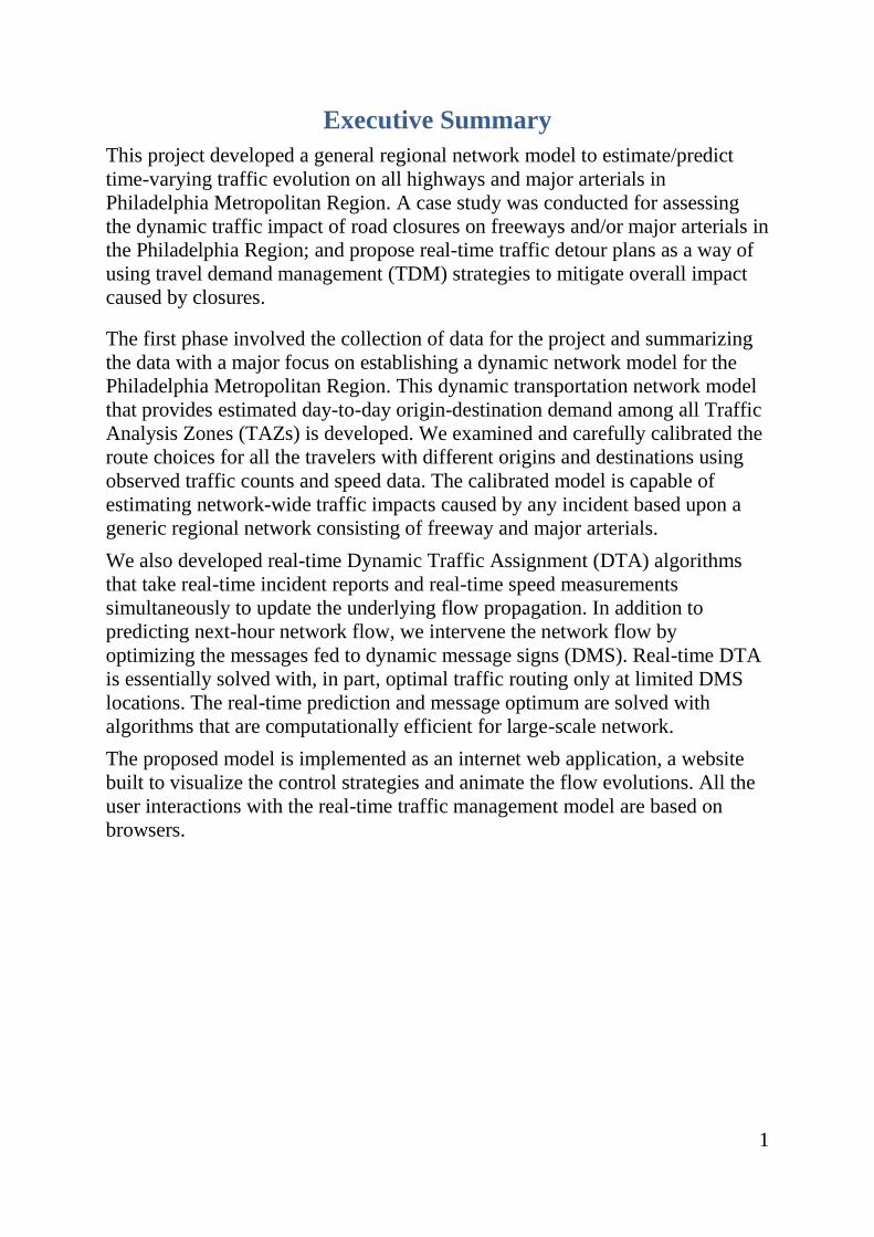
Executive Summary
This project developed a general regional network model to estimate/predict
time-varying traffic evolution on all highways and major arterials in
Philadelphia Metropolitan Region. A case study was conducted for assessing
the dynamic traffic impact of road closures on freeways and/or major arterials in
the Philadelphia Region; and propose real-time traffic detour plans as a way of
using travel demand management (TDM) strategies to mitigate overall impact
caused by closures.
The first phase involved the collection of data for the project and summarizing
the data with a major focus on establishing a dynamic network model for the
Philadelphia Metropolitan Region. This dynamic transportation network model
that provides estimated day-to-day origin-destination demand among all Traffic
Analysis Zones (TAZs) is developed. We examined and carefully calibrated the
route choices for all the travelers with different origins and destinations using
observed traffic counts and speed data. The calibrated model is capable of
estimating network-wide traffic impacts caused by any incident based upon a
generic regional network consisting of freeway and major arterials.
We also developed real-time Dynamic Traffic Assignment (DTA) algorithms
that take real-time incident reports and real-time speed measurements
simultaneously to update the underlying flow propagation. In addition to
predicting next-hour network flow, we intervene the network flow by
optimizing the messages fed to dynamic message signs (DMS). Real-time DTA
is essentially solved with, in part, optimal traffic routing only at limited DMS
locations. The real-time prediction and message optimum are solved with
algorithms that are computationally efficient for large-scale network.
The proposed model is implemented as an internet web application, a website
built to visualize the control strategies and animate the flow evolutions. All the
user interactions with the real-time traffic management model are based on
browsers.
2
Abbreviations
API: Application Programming Interface
BUE: Boston User Equilibrium
CTM: Cell Transmission Model
DODE: Dynamic Origin-Destination Estimation
DTA: Dynamic Traffic Assignment
DMS: Dynamic Message Signs
DVRPC: Delaware Valley Regional Planning Commission
LPFE: Logit Path Flow Estimator
O-D: Origin-Destination
PUE: Predictive User Equilibrium
RMSE: Root Mean Square Error
TAZ: Traffic Analysis Zones
TDM: Travel Demand Management
TMC: Traffic Message Channel
UE: User Equilibrium
VHT: Vehicle Hours Traveled
VMT: Vehicle Miles Traveled
3
1 Introduction
Non-recurrent traffic congestion caused by roadway construction work, planned
events, and unplanned traffic incidents can create massive traffic tie-ups and can
have equally large economic and environmental regional impacts. More
roadway rehabilitation/reconstruction work has been conducted over the recent
years on heavily travelled urban corridors which are already “capacity-hungry”.
With the availability of various traffic data to identify congestion (real-time and
historically archived), how to minimize incident-induced disruption to
commuting traffic and its impact to the environment presents a big challenge to
public agencies. While planned and unplanned incidents require careful
evaluation of alternative construction plans and corresponding traffic
management plans, guidelines to develop efficient traffic demand management
strategies are often lacking. Consequently, there is a real need to study planned
and unplanned traffic incidents to learn valuable lessons to prepare public
agencies to deal more effectively with large routine highway maintenance,
reconstruction, big sports events, catastrophic vehicle crash and emergency
situations.
The Philadelphia Metropolitan Region is traffic data rich compared to other
metropolitan areas in the U.S. Various data sets in the Philadelphia region,
including traditional traffic sensors (loops, cameras, etc.) and cutting-edge
sensors (Bluetooth, GPS probe, parking, etc.), are available and have been
archived for a decade. The rich data sets allow us to learn travelers’ behavior
more accurately and develop an in-depth understanding of non-recurrent traffic
in large-scale networks, which is usually influenced by abnormal disruptions
(such as incidents, events, weather, etc.).
Therefore we want to develop a general regional network model to
estimate/predict time-varying traffic evolution on all highways and major
arterials in Philadelphia Metropolitan Region. We accomplish this by
conducting a case study for I-95 closures, assessing the dynamic traffic impact
of the closures on both freeways and major arterials in the Philadelphia Region;
and propose real-time traffic detour plans as a way of using travel demand
management (TDM) strategies to mitigate overall impact caused by closures.
The purposes of the project are:
Develop a generic regional network model to estimate/predict time-
varying traffic evolution on all highways and major arterials in
Philadelphia Metropolitan Region. The model estimates origin-
destination demands within the region and captures travel behavior of
those travelers (in particular their time-varying route choices).
Conduct a case study for Center City bridge closures: assess the dynamic
traffic impact of Center City Bridge closures on both freeways and major
4
arterials in the Philadelphia Region; propose real-time traffic detour plans
as a way of travel demand management (TDM) to mitigate overall impact
caused by closures. The traffic detour plans include optimized traffic
signal timing on major intersections and on-site detour strategies through
Dynamic Message Signs (DMS).
Conduct a second case study for hypothetical I-95 closures: assess traffic
impact of I-95 closures in Downtown Philadelphia and prepare traffic
detour plans.
The remainder of this report is organized as follows.
Section 2 briefly reviews the cutting-edge off-line and on-line dynamic
traffic network models.
Section 3 summarizes and describes the road network files and date we
obtained.
Section 4 describes the procedures of constructing the network and pre-
processing the traffic data.
Section 5 presents the model details of the off-line dynamic traffic
assignment model on Philadelphia Metropolitan Region.
Section 6 presents the model details of the on-line dynamic traffic
assignment model on Philadelphia Metropolitan Region.
5
2. Model review
As an emerging technology in transportation area, Dynamic Traffic Assignment
(DTA) plays a vital role for real-time traffic management and planning. DTA
consists of various kinds of sub-models such as dynamic routing, traffic flow
evolution theory, travel behavior model and economic models (Peeta &
Ziliaskopoulos 2001). There are two main components in the DTA families, off-
line DTA and on-line DTA. Off-line DTA collects the data before learning the
travelers’ behavior and simulating traffic. While the on-line DTA model
collects the real time data as the simulation goes. It uses the real-time data to
correct the estimation of demand and behavior on the fly, and there is usually
more challenging. The off-line DTA model is usually used for traffic
planning/operation, whereas the on-line DTA model is used for real-time traffic
prediction and management.
In this section, we build both off-line DTA model and real-time DTA for the
Philadelphia Metropolitan Region and analyze the traffic impact of road
closures. To familiarize readers the development of DTA models, we present a
brief literature review on some important issues on simulation-based DTA
models and discuss several cutting-edge on-line and off-line DTA models.
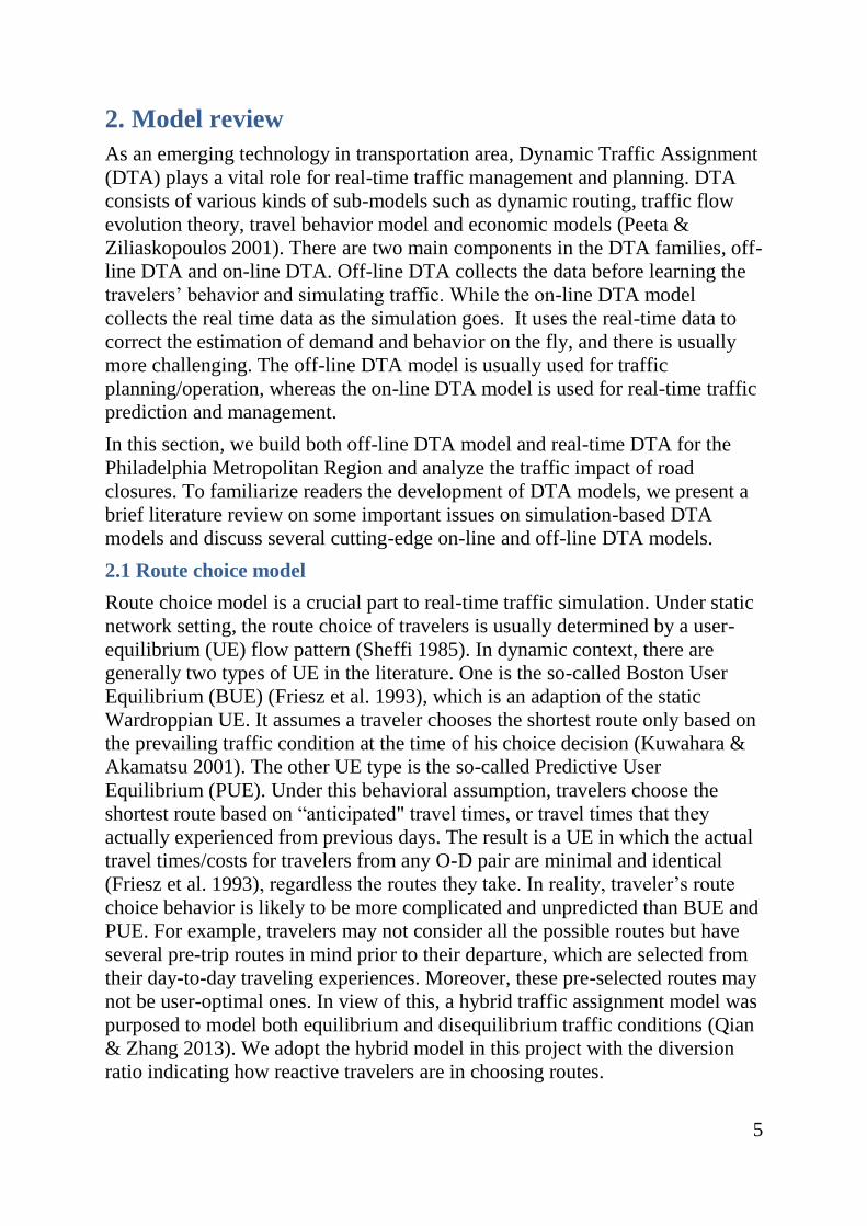
2.1 Route choice model
Route choice model is a crucial part to real-time traffic simulation. Under static
network setting, the route choice of travelers is usually determined by a user-
equilibrium (UE) flow pattern (Sheffi 1985). In dynamic context, there are
generally two types of UE in the literature. One is the so-called Boston User
Equilibrium (BUE) (Friesz et al. 1993), which is an adaption of the static
Wardroppian UE. It assumes a traveler chooses the shortest route only based on
the prevailing traffic condition at the time of his choice decision (Kuwahara &
Akamatsu 2001). The other UE type is the so-called Predictive User
Equilibrium (PUE). Under this behavioral assumption, travelers choose the
shortest route based on “anticipated" travel times, or travel times that they
actually experienced from previous days. The result is a UE in which the actual
travel times/costs for travelers from any O-D pair are minimal and identical
(Friesz et al. 1993), regardless the routes they take. In reality, traveler’s route
choice behavior is likely to be more complicated and unpredicted than BUE and
PUE. For example, travelers may not consider all the possible routes but have
several pre-trip routes in mind prior to their departure, which are selected from
their day-to-day traveling experiences. Moreover, these pre-selected routes may
not be user-optimal ones. In view of this, a hybrid traffic assignment model was
purposed to model both equilibrium and disequilibrium traffic conditions (Qian
& Zhang 2013). We adopt the hybrid model in this project with the diversion
ratio indicating how reactive travelers are in choosing routes.
6
2.2 Flow evolution model
The flow evolution models describe the dynamic relationship between vehicle
density, speed and volume for one road segment. Three models are most
adopted by various mesoscopic traffic simulation tools: Point Queue (PQ) (Jin
2015), Spatial Queue (SQ) (Balmer et al. 2004; Breuer 2001) and Cell
Transmission Model (CTM) (Daganzo 1995; Daganzo 1999). Though
mathematically and practically simple, PQ and SQ are considered to
underestimate the network congestion during the simulation (Zhang et al. 2013).
CTM as a finite element approximation to the partial differential equation of
fluid evolution is proved to best simulate the flow propagation on road segments.
A vital issue exists for all dynamic flow evolution models, which is the
unrealistic “gridlock” caused by improper routing behavior and misbehave of
flow evolution models (Mahmassani et al. 2013).
In this project, we adopt CTM to simulate the flow propagation on links, and the
unrealistic gridlock condition is eliminated by calibrating behavior model
parameters and network dynamic features.
2.3 Off-line DTA
Off-line DTA models have been thoroughly studied in recent years. According
to the simulation resolution, there are three types: macroscopic, microscopic and
mesoscopic DTA models. Mesoscopic model is considered to have great
potentials for large-scale network simulation with satisfactory precisions. Two
pioneers of mesoscopic off-line DTA are DNASMART (Jayakrishnan et al.
1994) and DYNAMIT (Ben-akiva et al. 1998). Both softwares utilize density-
speed relationship function to calculate the position of vehicle and simulation
the flow propagation, so they do not need to keep track of all vehicles. This
simplification significantly reduces the computational complexity.
For all off-line DTA models, an important issue is the trade-off between the
simulation accuracy and running time. If a high accuracy is needed, then the
running time will be almost implausible for large scale networks. Therefore, we
need to tune the best simulation resolution as a compromise between
computational efficiency and accuracy.
2.4 On-line DTA
While emerging Advanced Traveler Information Systems/Advanced Traffic
Management Systems (ATIS/ATMS) technologies (Mahmassani 1998; Ben-
Akiva et al. 1991), which search for routing policies for travelers to achieve
real-time network-wise optimum, require the DTA models take on-line data
feeds and update management strategies in real time. DTA models that can take
real-time data feeds is known as on-line DTA or real-time DTA. Researches of
real-time DTA arise accordingly from different disciplines. After two decades’
development, real-time DTA models formulate various control mechanisms
7
which take different kinds of data feeds (travel time, traffic flow), adopt various
controls (ramp metering, signal timing, VMS, routing) and achieve different
objectives (user equilibrium, system optimal).
The idea of real-time DTA originates from the field of optimal control, which
assumes the observations of network are complete and travel demands and
supplies are pre-determined. Studies (Papageorgiou 1990) build a node based
DTA model and control the splitting rate to achieve system optimal or user
equilibrium, linearization regulation of the original non-linear DTA model is
also developed to handle the large scale network. They also develop
METANET as a traffic routing and control framework. Similar real-time DTA
problem is also settled by adjusting point diversion using linearization (Kachroo
& Özbay 1998). Instead of open-loop framework, (Kachroo & Özbay 2005)
further formulate a H∞ closed-loop feed-back control mechanism on splitting
rate. Many other studies also attempt to dynamically control traffic by ramp
metering (Zhang et al. 2001), signal timing (Mirchandani & Head 2001; Yang
& Yagar 1995), routing guidance (Jahn et al. 2005) and dynamic message sign
(DMS) (Shi et al. 2009; Mammar et al. 1996). Among them (Papageorgiou
1995) provides an integrated framework to control traffic flows using all above
methods.
In real world, only partial network conditions can be observed and travel
demands and supplies are usually unknown. Current/future traffic conditions are
estimated/predicted and then reactive/predictive control are applied (Doan &
Ziliaskopoulos n.d.). There are literature (Van Arem et al. 1993; Wang &
Papageorgiou 2005) focusing on calibrating the supply parameters such as road
capacity. Techniques such as ARMA (Hashemi & Abdelghany 2015), Kalman
Filter (Wang & Papageorgiou 2005; Antoniou 2004) are also adopted in various
models to predict future traffic conditions. Recently an approach called ``rolling
horizon" is adopted to tackle network-wise general real-time traffic problem
based on simulation software such as DYNASMART (Peeta & Mahmassani
1995; Samaranayake et al. 2015), DynaMIT (Ben-Akiva & Bierlaire 2001),
DynusT (Chiu & Mirchandani 2008). The methods estimate current traffic
conditions and predict future conditions in each time interval (Zhou &
Mahmassani 2007; Mahmassani 2001; Antoniou 2004), then the control policies
are determined by the estimated/predicted traffic condition (Li et al. 2015; Du et
al. 2014).
Some of real-time DTA models are also implemented in commercial software
such as PTV Optima1 and Aimsun2. Both softwares are able to provide real time
1 http://vision-traffic.ptvgroup.com/en-uk/products/ptv-optima/
2 https://www.aimsun.com/

8
information and provide forecasts on traffic conditions of entire networks.
Aimsun has already built an Integrated Corridor Management (ICM) system
within the I-15 corridor in San Diego County. The whole ICM system is fully
automatic and equipped with various combinations of strategies such traveler
information platform, traffic management and transit management.
In this project, we develop a framework that takes the real time vehicle speed
data feed as inputs and update the real-time O-D demand, as well as routing
behavior. The predicted travel time along with routing guidance
recommendation will be disseminated to the travelers by Variable Message
Signs (VMS) and radio broadcasts. The model will be specially tailored for
applications to the Philadelphia Metropolitan Region.
9
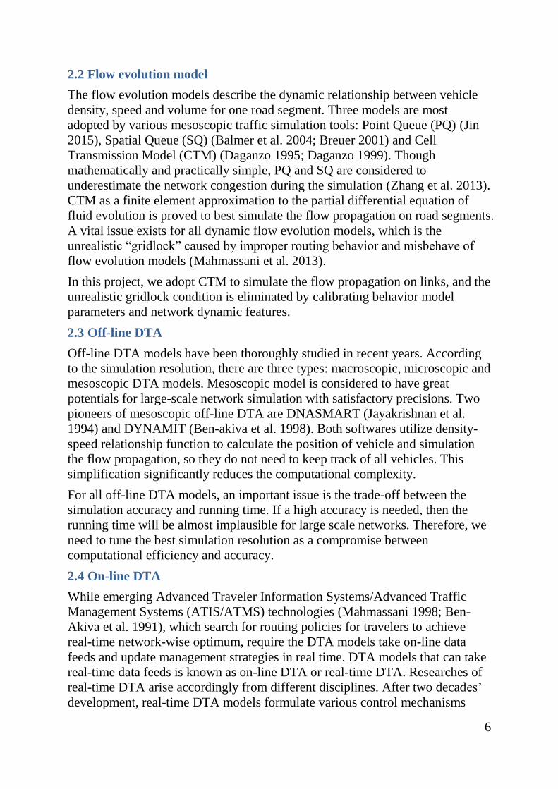
3. Data summary
Figure 1 DVRPC Regional Map (retrieved from DVRPC website)
Data from nine counties in the Delaware Valley Regional Planning Commission
(DVRPC) region were collected for this project. Figure 13 shows the
geographical boundaries of the DVRPC region. Data obtained includes network
topological data, historical O-D, traffic counts and traffic speeds. Since they
were collected from different sources, we briefly discuss the format and
contents for each data.
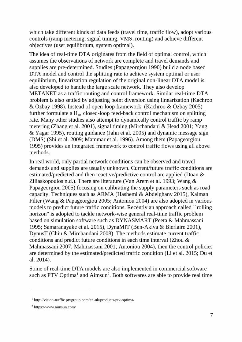
3.1 Network topological data
The nine-county network was obtained from DVRPC in the format of PTV
Visum. The file contains 3,399 traffic analysis zones (TAZ), 90,083 junctions
and 255,992 road segments. The network includes Bucks, Chester, Delaware,
Montgomery and Philadelphia counties in Pennsylvania; and Burlington,
Camden, Gloucester and Mercer counties in New Jersey. Figure 2 is a
screenshot of the obtained network, and the colors represent different road
levels. The road segments have attributes such as street names, street levels
(highway, major arterials, minor streets, alleys, etc.), number of lanes, and
speed limit.
Together with the network file, the regional travel planning model (TIM2.1)
from DVRPC was also contained in the same data file. The static traffic
assignment model may help build our dynamic analytic model.
3 http://www.dvrpc.org/img/homepage/DVRPC_Regional_Map.png, retrieved on 28th Oct 2015.
10
Figure 2 Screenshot of DVRPC network
3.2 History O-D
The historical O-D demand data was also obtained from DVRPC in the format
of VISUM. The O-D matrix is represented by a 3399 × 3399 matrix and in
float precision. DVRPC also provided a main O-D pairs profile, which contains
10,000 main O-Ds. O-D connectors are also contained in the TIM2.1 model, the
total number of O-D connectors is 11,553,201.
3.3 Traffic counts
DVRPC provided us with 15-minute interval traffic volume counts data from 3rd
Jan 2013 to 15th Oct 2015. The data file has 568,524 rows; each row indicates
the count of a 15-minute period on a certain day collected by a loop detector on
various roadway segments. There are in all 3,565 different detectors, each
detector has the information of its geographic location (latitude and longitude),
and road name. However, the dates when those measurements were collected
vary throughout the year.
3.4 Traffic speed
Travel speed data provided by INRIX were obtained from the Regional
Integrated Transportation Information System (RITIS). The data set includes
13,104 Traffic Management Channels (TMCs) for the nine counties of DVRPC.
The data includes speed, travel time, historic average speed and reference speed
(namely 85% quantile of all observed probe vehicle speeds, used as the free-
flow speed). All data are averaged into 15 minute intervals to meet the needs of
our dynamic analytic model.
11
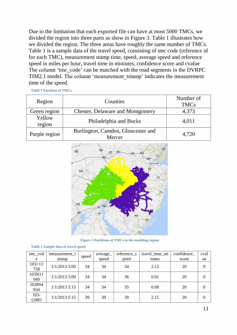
Due to the limitation that each exported file can have at most 5000 TMCs, we
divided the region into three parts as show in Figure 3. Table 1 illustrates how
we divided the region. The three areas have roughly the same number of TMCs.
Table 1 is a sample data of the travel speed, consisting of tmc code (reference id
for each TMC), measurement stamp time, speed, average speed and reference
speed in miles per hour, travel time in miniutes, confidence score and cvalue
The column ‘tmc_code’ can be matched with the road segments in the DVRPC
TIM2.1 model. The column ‘measurement_tstamp’ indicates the measurement
time of the speed.
Table 1 Partition of TMCs
Region Counties Number of
TMCs
Green region Chester, Delaware and Montgomery 4,373
Yellow
region Philadelphia and Bucks 4,011
Purple region Burlington, Camden, Gloucester and
Mercer 4,720
Figure 3 Partitions of TMCs in the modeling region
Table 2 Sample data of travel speed
tmc_cod
e
measurement_t
stamp speed
average_
speed
reference_s
peed
travel_time_mi
nutes
confidence_
score
cval
ue
103+13
758 1/1/2013 5:00 34 34 34 2.12 20 0
103N11
940 1/1/2013 5:00 34 34 36 0.01 20 0
103P04
934 1/1/2013 5:15 34 34 35 0.08 20 0
103-
12881 1/1/2013 5:15 39 39 39 2.15 20 0

12
3.5 Dynamic message sign (DMS)
All the information about dynamic message signs on Philadelphia Metropolitan
Region is provided by DVRPC. A brief description of the location of DMS and
the coordinates are given in the file. The file also specifies the suggest detour
link the DMSs.
13
4. Data preparation
Network description files and traffic data sets for the nine counties of Delaware
Valley Regional Planning Commission (DVRPC) region were collected for this
project. The network description files are trimmed, consolidated and further
coded into our state-of-art traffic simulation tools, and the traffic data sets are
processed, smoothed and matched to each road segments.
4.1 Network description
The network for Philadelphia Metropolitan Area is from the Delaware Valley
Regional Planning Commission (DVRPC) in the format of PTV Visum. The file
contains 3,399 traffic analysis zones (TAZ), 90,083 junctions and 255,992 road
segments. The network includes Bucks, Chester, Delaware, Montgomery and
Philadelphia counties in Pennsylvania; and Burlington, Camden, Gloucester and
Mercer counties in New Jersey. Figure 4 is a screenshot of the obtained network,
and the colors represent different road levels. The road segments have attributes
such as street names, street levels (highway, major arterials, minor streets,
alleys, etc.), number of lanes, and speed limits.
A network consolidation was conducted to trim the original network. The
following steps were carried out to conduct the consolidation before the
simulation:
We consolidated the network according to the road levels. The entire
network was divided into 3 parts, for those areas far away from
Philadelphia County, we retain the highways; for those areas neighbored
with Philadelphia County, we retain the highways and major arterials;
and we retain all the roads inside the Philadelphia County.
The network was then trimmed such that no “isolated" nodes and links
exist. “Isolated" nodes are those who have only one forward link and one
backward link, and the head node of the forward link is exactly the tail
node of the backward link. Further, “isolated" links are the forward links
and backward links of “isolated" nodes. The absence of such nodes and
links does not affect the dynamic network analysis, but allows for a more
precise estimation of network performance indicators.
We consolidated neighboring links with small lengths and the same speed
limit. This process substantially reduced the network scale. More
importantly, this was desirable to achieve more accuracy for the
mesoscopic traffic flow models.
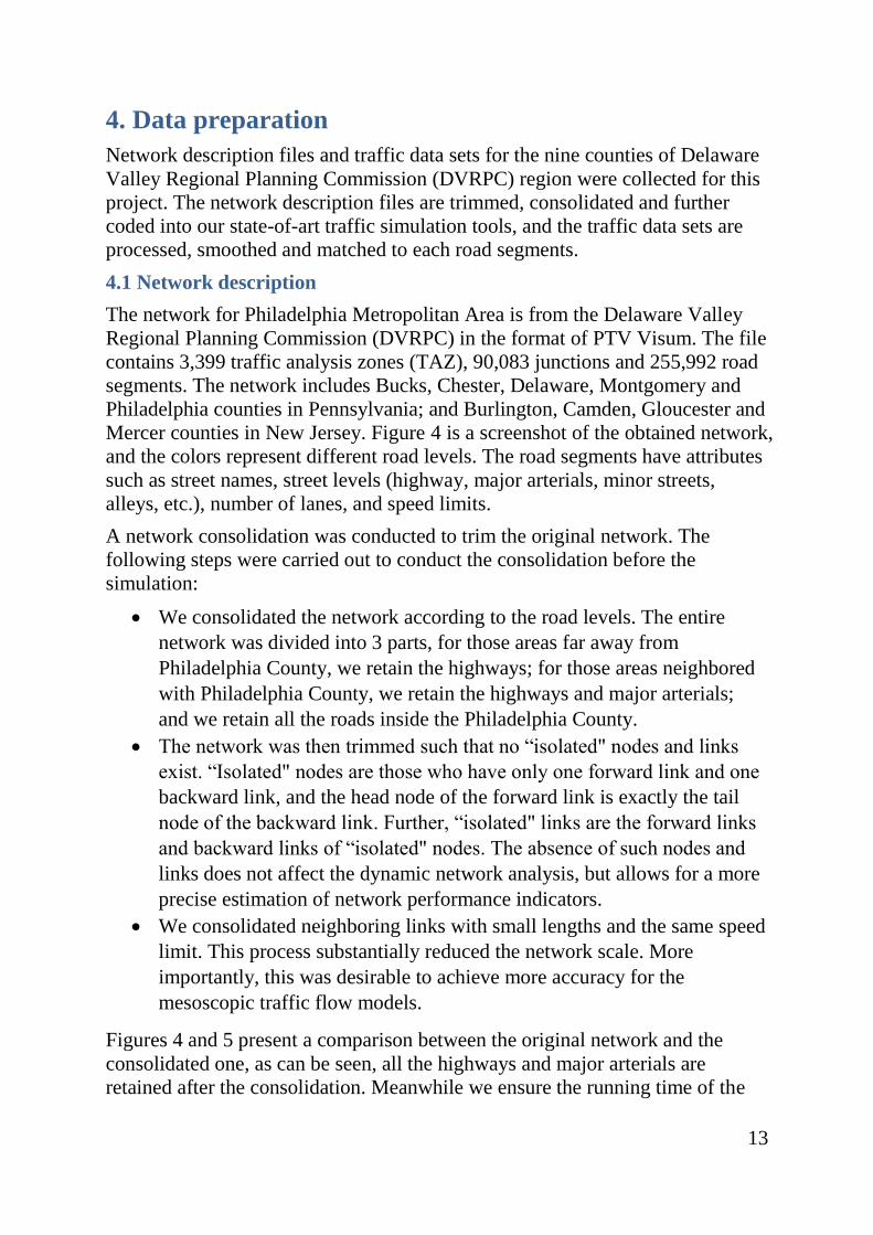
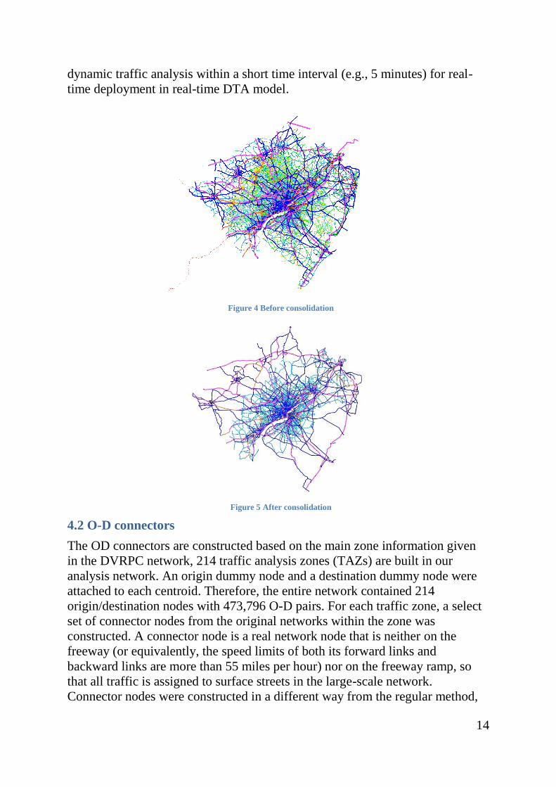
Figures 4 and 5 present a comparison between the original network and the
consolidated one, as can be seen, all the highways and major arterials are
retained after the consolidation. Meanwhile we ensure the running time of the
14
dynamic traffic analysis within a short time interval (e.g., 5 minutes) for real-
time deployment in real-time DTA model.
Figure 4 Before consolidation
Figure 5 After consolidation
4.2 O-D connectors
The OD connectors are constructed based on the main zone information given
in the DVRPC network, 214 traffic analysis zones (TAZs) are built in our
analysis network. An origin dummy node and a destination dummy node were
attached to each centroid. Therefore, the entire network contained 214
origin/destination nodes with 473,796 O-D pairs. For each traffic zone, a select
set of connector nodes from the original networks within the zone was
constructed. A connector node is a real network node that is neither on the
freeway (or equivalently, the speed limits of both its forward links and
backward links are more than 55 miles per hour) nor on the freeway ramp, so
that all traffic is assigned to surface streets in the large-scale network.
Connector nodes were constructed in a different way from the regular method,
15
because trips are most likely to start and end on local streets. In addition, we
made three or four connections between real network nodes (in the selection set)
and those dummy nodes, rather than those centroids directly. This method
ensures through traffic will never unrealistically use connectors to reduce travel
time.
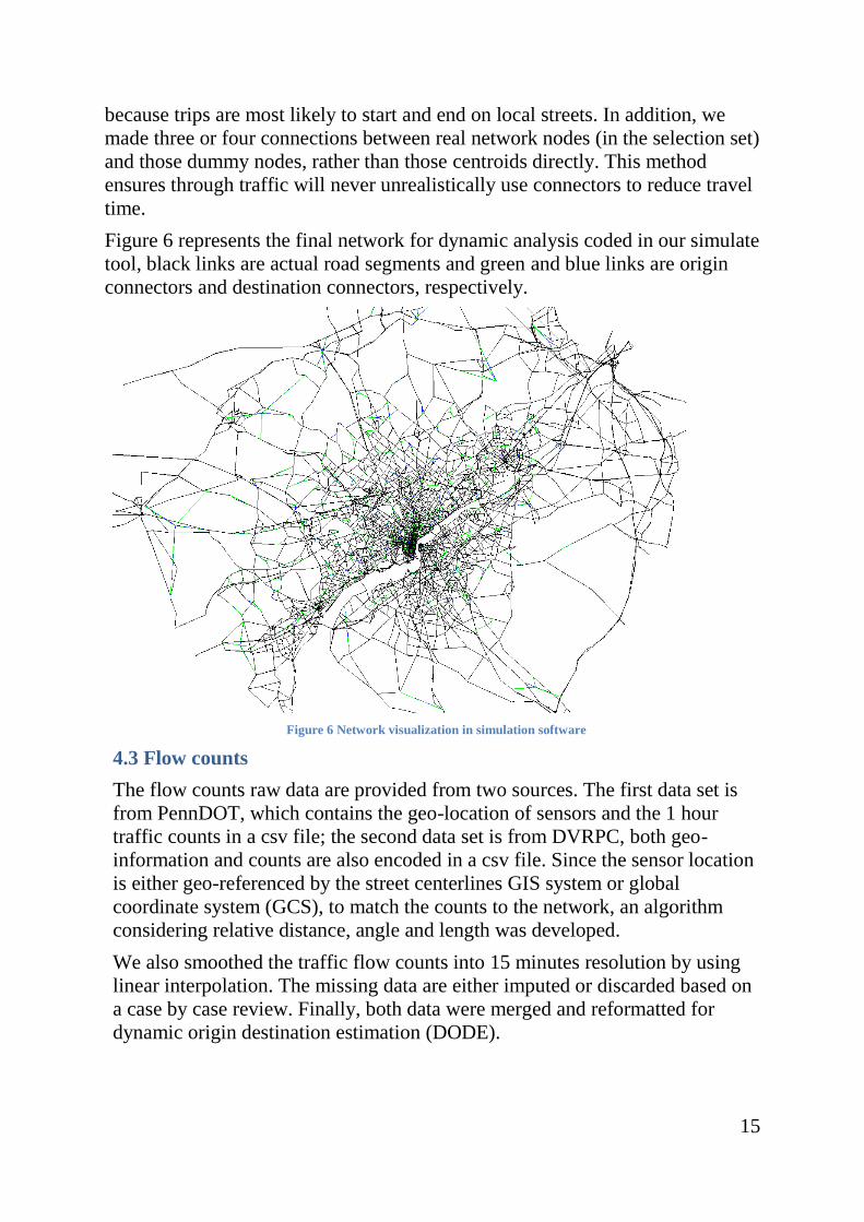
Figure 6 represents the final network for dynamic analysis coded in our simulate
tool, black links are actual road segments and green and blue links are origin
connectors and destination connectors, respectively.
Figure 6 Network visualization in simulation software
4.3 Flow counts
The flow counts raw data are provided from two sources. The first data set is
from PennDOT, which contains the geo-location of sensors and the 1 hour
traffic counts in a csv file; the second data set is from DVRPC, both geo-
information and counts are also encoded in a csv file. Since the sensor location
is either geo-referenced by the street centerlines GIS system or global
coordinate system (GCS), to match the counts to the network, an algorithm
considering relative distance, angle and length was developed.
We also smoothed the traffic flow counts into 15 minutes resolution by using
linear interpolation. The missing data are either imputed or discarded based on
a case by case review. Finally, both data were merged and reformatted for
dynamic origin destination estimation (DODE).
16
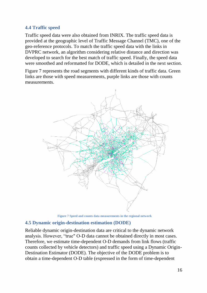
4.4 Traffic speed
Traffic speed data were also obtained from INRIX. The traffic speed data is
provided at the geographic level of Traffic Message Channel (TMC), one of the
geo-reference protocols. To match the traffic speed data with the links in
DVPRC network, an algorithm considering relative distance and direction was
developed to search for the best match of traffic speed. Finally, the speed data
were smoothed and reformatted for DODE, which is detailed in the next section.
Figure 7 represents the road segments with different kinds of traffic data. Green
links are those with speed measurements, purple links are those with counts
measurements.
Figure 7 Speed and counts data measurements in the regional network
4.5 Dynamic origin-destination estimation (DODE)
Reliable dynamic origin-destination data are critical to the dynamic network
analysis. However, “true" O-D data cannot be obtained directly in most cases.
Therefore, we estimate time-dependent O-D demands from link flows (traffic
counts collected by vehicle detectors) and traffic speed using a Dynamic Origin-
Destination Estimator (DODE). The objective of the DODE problem is to
obtain a time-dependent O-D table (expressed in the form of time-dependent
17
path flows) that, once loaded onto the network, will reproduce observed link
traffic counts and other observations as closely as possible.
4.5.1 Methodology
We adopt Logit Path Flow Estimator (LPFE) to derive path flows (hence an
estimation of O-D demands). LPFE borrows the ideas of stochastic traffic
assignment models which recognize that travelers are unlikely to get perfect
information about network conditions. Therefore it is considered to be able to
model individuals' route choice behaviors more realistically.
In this project, the complete observations of traffic flows and speeds are
obtained (under healthy conditions) from 1992 road segments. We estimated
time-dependent O-D demands in 15 minute interval based on flow count data.
We verified the accuracy of the estimated O-D demands by comparing the
estimated link flow (based on estimated O-D demands) to the observed link ow
(input).
The O-D demands for both AM peak and PM peak are estimated separately by
using data inputs from different time of day. The total number of travel demand
in PM is significantly higher than in AM, therefore we can conjecture that the
network will get more congested during the PM peak.
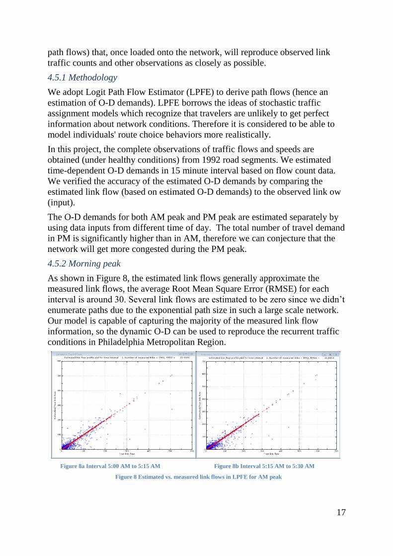
4.5.2 Morning peak
As shown in Figure 8, the estimated link flows generally approximate the
measured link flows, the average Root Mean Square Error (RMSE) for each
interval is around 30. Several link flows are estimated to be zero since we didn’t
enumerate paths due to the exponential path size in such a large scale network.
Our model is capable of capturing the majority of the measured link flow
information, so the dynamic O-D can be used to reproduce the recurrent traffic
conditions in Philadelphia Metropolitan Region.
Figure 8a Interval 5:00 AM to 5:15 AM Figure 8b Interval 5:15 AM to 5:30 AM
Figure 8 Estimated vs. measured link flows in LPFE for AM peak
18
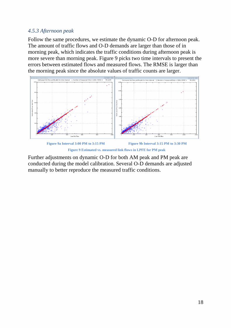
4.5.3 Afternoon peak
Follow the same procedures, we estimate the dynamic O-D for afternoon peak.
The amount of traffic flows and O-D demands are larger than those of in
morning peak, which indicates the traffic conditions during afternoon peak is
more severe than morning peak. Figure 9 picks two time intervals to present the
errors between estimated flows and measured flows. The RMSE is larger than
the morning peak since the absolute values of traffic counts are larger.
Figure 9a Interval 3:00 PM to 3:15 PM Figure 9b Interval 3:15 PM to 3:30 PM
Figure 9 Estimated vs. measured link flows in LPFE for PM peak
Further adjustments on dynamic O-D for both AM peak and PM peak are
conducted during the model calibration. Several O-D demands are adjusted
manually to better reproduce the measured traffic conditions.
19
5. Off-line DTA for Philadelphia Metropolitan Region
The regional network, together with construction/road closure plans of I-95
corridor, is coded into the dynamic network model. Baseline travel demand is
estimated in the first place using the integrated traffic data (counts, INRIX data)
on typical weekdays without the presence of large incidents. Under the actual I-
95 corridor construction/road closure plans, the change of traffic conditions can
be estimated by simulating traffic in the calibrated dynamic network.
Two time windows are analyzed for the Philadelphia Metropolitan Region: the
AM peak and PM peak. AM peak represents the time horizon from 5AM to
10AM in the morning, and PM peak represents 3PM to 8PM in the afternoon.
The overall traffic impact for each scenario without deploying any real-time
traffic management strategies can be measured by time-of-day traffic evolution
in the region, as well as performance metrics, such as total traffic delay, average
travel time, emissions, energy use, vehicle-miles travelled, etc.
Detailed information for each road segment is also available after applying the
model. The most impacted highways and arterials under each scenario are
identified, along with possible explanations and suggestions. Travel times
between selected origin-designation pairs in each scenario are also compared to
gain for insights and prediction power.
5.1 Methodology
A mesoscopic network simulation framework is used to evaluate the network
under different settings. Before the simulation can be done, we need to calibrate
the model with the observed data. We tune the properties of road segments such
that the simulation results are consistent with the obtained speed/counts data in
those measured locations.
Additionally, it is possible that the simulation terminates unsuccessfully because
sometimes the network loading produces “grid-lock", a notorious condition
defined as the inability of vehicles to move. This is a common issue in
mesoscopic network simulation and will lead the simulation to fail.
By trial-and-error, we calibrated the parameters of link properties and routing
behavior such that the simulations can succeed without a gridlock and
meanwhile produce traffic conditions as close as possible to the observed data.
In the remaining part of this section, the simulation results on the calibrated
network will be presented. After the calibration work, we see that the simulation
model yields good results.
5.2 Morning peak
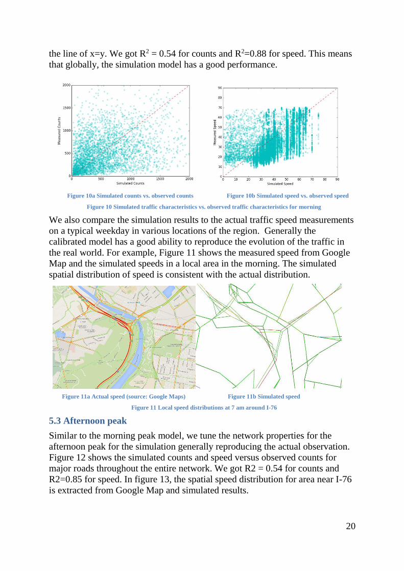
Figure 10 shows the simulated counts and speed versus observed counts for
major roads throughout the entire network. Ideally, the scatter should be around
20
the line of x=y. We got R2 = 0.54 for counts and R2=0.88 for speed. This means
that globally, the simulation model has a good performance.
Figure 10a Simulated counts vs. observed counts Figure 10b Simulated speed vs. observed speed
Figure 10 Simulated traffic characteristics vs. observed traffic characteristics for morning
We also compare the simulation results to the actual traffic speed measurements
on a typical weekday in various locations of the region. Generally the
calibrated model has a good ability to reproduce the evolution of the traffic in
the real world. For example, Figure 11 shows the measured speed from Google
Map and the simulated speeds in a local area in the morning. The simulated
spatial distribution of speed is consistent with the actual distribution.
Figure 11a Actual speed (source: Google Maps) Figure 11b Simulated speed
Figure 11 Local speed distributions at 7 am around I-76
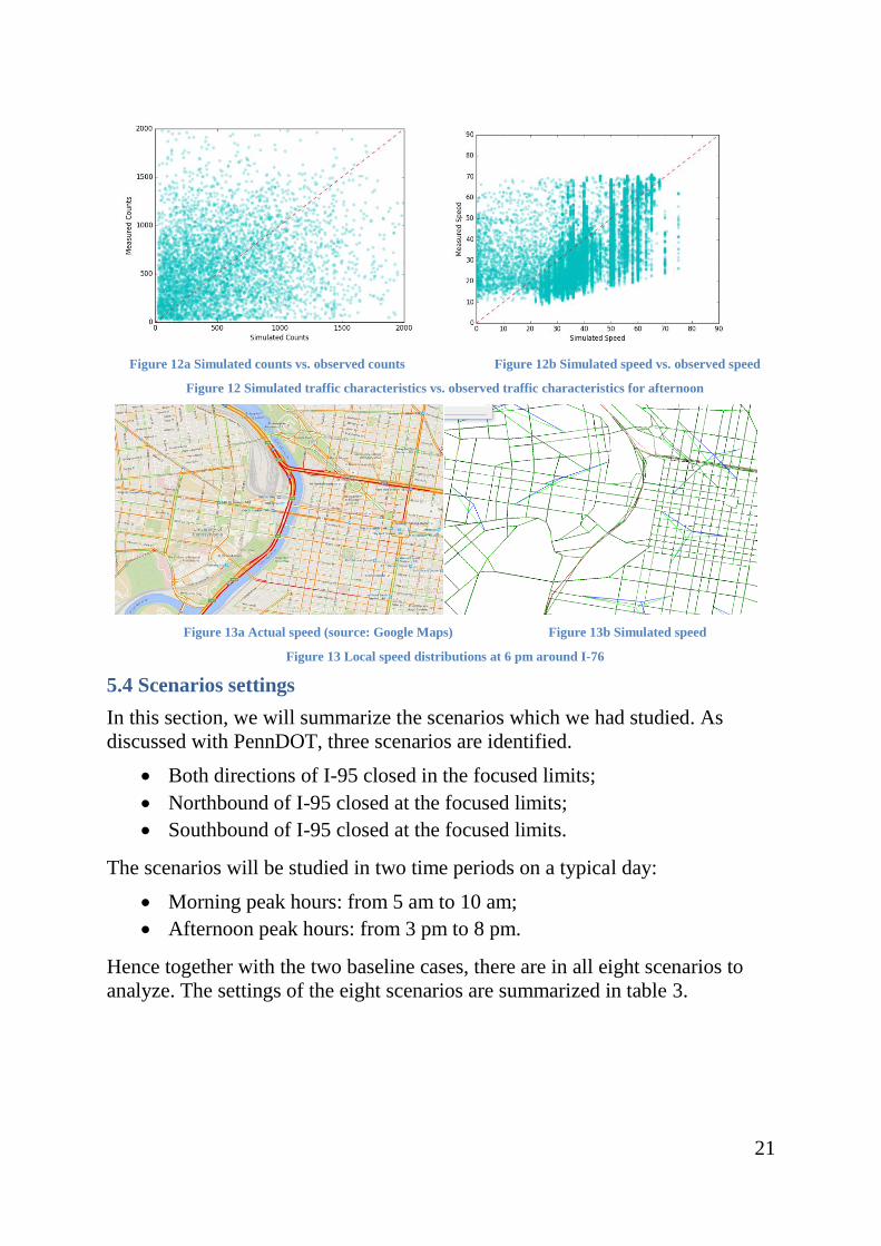
5.3 Afternoon peak
Similar to the morning peak model, we tune the network properties for the
afternoon peak for the simulation generally reproducing the actual observation.
Figure 12 shows the simulated counts and speed versus observed counts for
major roads throughout the entire network. We got R2 = 0.54 for counts and
R2=0.85 for speed. In figure 13, the spatial speed distribution for area near I-76
is extracted from Google Map and simulated results.
21
Figure 12a Simulated counts vs. observed counts Figure 12b Simulated speed vs. observed speed
Figure 12 Simulated traffic characteristics vs. observed traffic characteristics for afternoon
Figure 13a Actual speed (source: Google Maps) Figure 13b Simulated speed
Figure 13 Local speed distributions at 6 pm around I-76
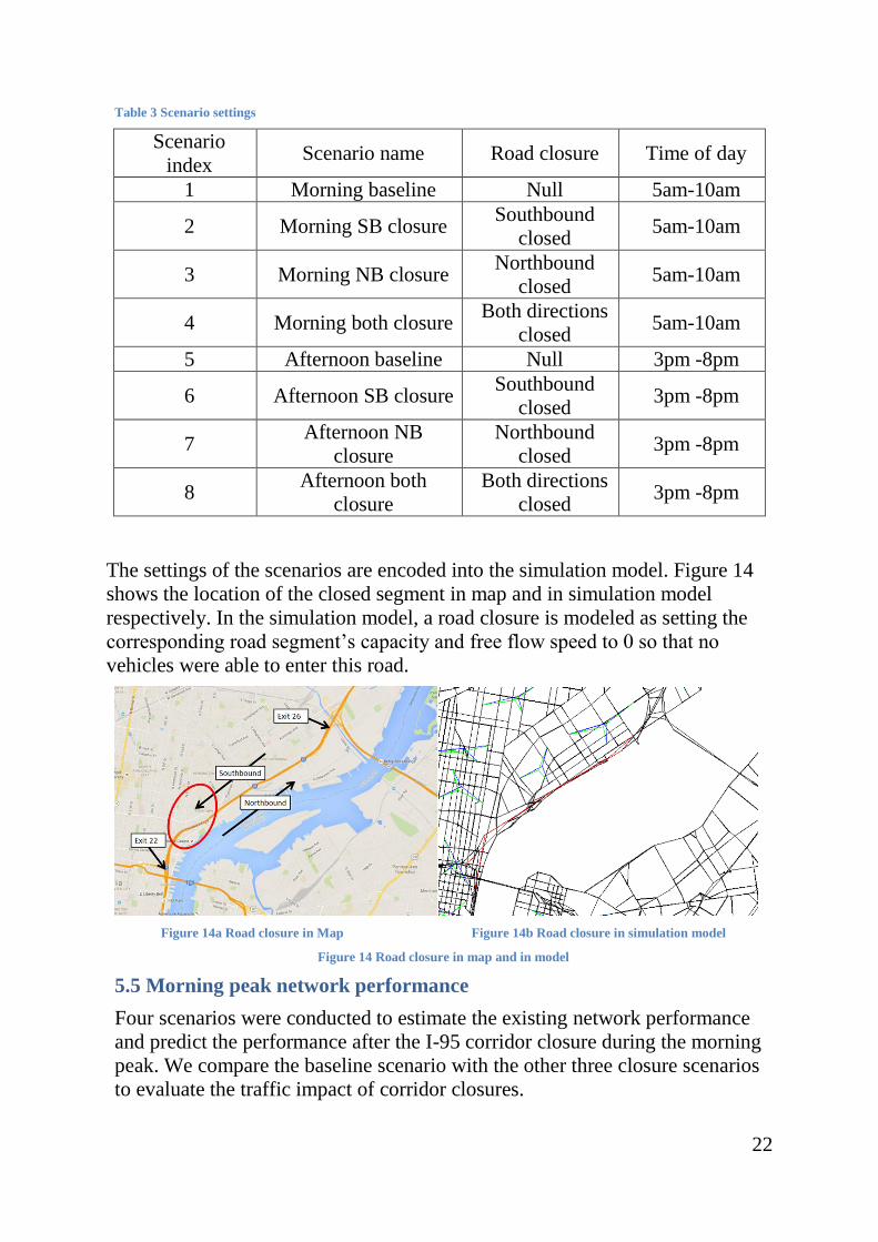
5.4 Scenarios settings
In this section, we will summarize the scenarios which we had studied. As
discussed with PennDOT, three scenarios are identified.
Both directions of I-95 closed in the focused limits;
Northbound of I-95 closed at the focused limits;
Southbound of I-95 closed at the focused limits.
The scenarios will be studied in two time periods on a typical day:
Morning peak hours: from 5 am to 10 am;
Afternoon peak hours: from 3 pm to 8 pm.
Hence together with the two baseline cases, there are in all eight scenarios to
analyze. The settings of the eight scenarios are summarized in table 3.
22
Table 3 Scenario settings
Scenario
index Scenario name Road closure Time of day
1 Morning baseline Null 5am-10am
2 Morning SB closure Southbound
closed 5am-10am
3 Morning NB closure Northbound
closed 5am-10am
4 Morning both closure Both directions
closed 5am-10am
5 Afternoon baseline Null 3pm -8pm
6 Afternoon SB closure Southbound
closed 3pm -8pm
7 Afternoon NB
closure
Northbound
closed 3pm -8pm
8 Afternoon both
closure
Both directions
closed 3pm -8pm
The settings of the scenarios are encoded into the simulation model. Figure 14
shows the location of the closed segment in map and in simulation model
respectively. In the simulation model, a road closure is modeled as setting the
corresponding road segment’s capacity and free flow speed to 0 so that no
vehicles were able to enter this road.
Figure 14a Road closure in Map Figure 14b Road closure in simulation model
Figure 14 Road closure in map and in model
5.5 Morning peak network performance
Four scenarios were conducted to estimate the existing network performance
and predict the performance after the I-95 corridor closure during the morning
peak. We compare the baseline scenario with the other three closure scenarios
to evaluate the traffic impact of corridor closures.
23
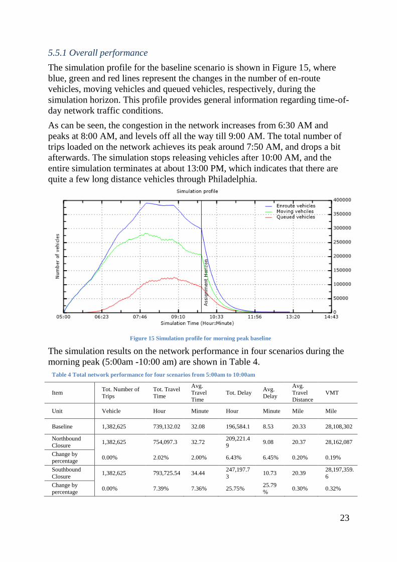
5.5.1 Overall performance
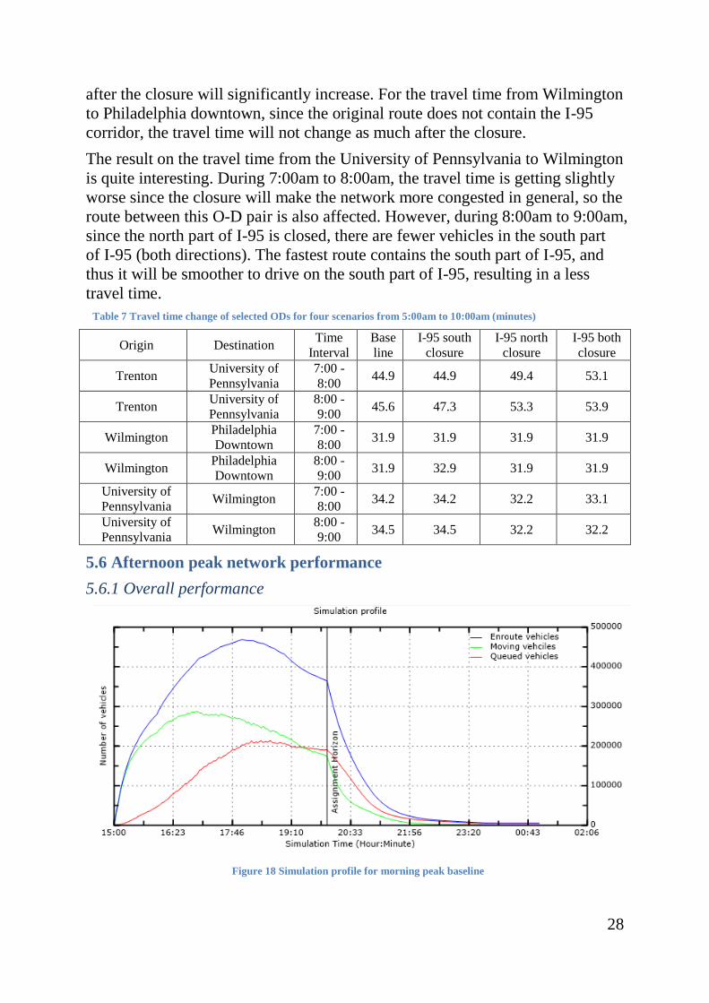
The simulation profile for the baseline scenario is shown in Figure 15, where
blue, green and red lines represent the changes in the number of en-route
vehicles, moving vehicles and queued vehicles, respectively, during the
simulation horizon. This profile provides general information regarding time-of-
day network traffic conditions.
As can be seen, the congestion in the network increases from 6:30 AM and
peaks at 8:00 AM, and levels off all the way till 9:00 AM. The total number of
trips loaded on the network achieves its peak around 7:50 AM, and drops a bit
afterwards. The simulation stops releasing vehicles after 10:00 AM, and the
entire simulation terminates at about 13:00 PM, which indicates that there are
quite a few long distance vehicles through Philadelphia.
Figure 15 Simulation profile for morning peak baseline
The simulation results on the network performance in four scenarios during the
morning peak (5:00am -10:00 am) are shown in Table 4.
Table 4 Total network performance for four scenarios from 5:00am to 10:00am
Item Tot. Number of
Trips
Tot. Travel
Time
Avg.
Travel
Time
Tot. Delay Avg.
Delay
Avg.
Travel
Distance
VMT
Unit Vehicle Hour Minute Hour Minute Mile Mile
Baseline 1,382,625 739,132.02 32.08 196,584.1 8.53 20.33 28,108,302
Northbound
Closure 1,382,625 754,097.3 32.72
209,221.4
9 9.08 20.37 28,162,087
Change by
percentage 0.00% 2.02% 2.00% 6.43% 6.45% 0.20% 0.19%
Southbound
Closure 1,382,625 793,725.54 34.44
247,197.7
3 10.73 20.39
28,197,359.
6
Change by
percentage 0.00% 7.39% 7.36% 25.75%
25.79
% 0.30% 0.32%
24
Both Closure 1,382,625 806,418.82 35 258,457.3
3 11.22 20.48 28,206,580
Change by
percentage 0.00% 9.10% 9.10% 31.47%
31.54
% 0.74% 0.35%
Generally, the network becomes more congested after the corridor closure. The
total number of trips remains the same, because we assume the traffic demands
are mainly composed of commuters who do not cancel trips in the morning peak.
The Vehicle-Mile-Traveled (VMT) and average travel distance will increase
since travelers may detour to a slightly longer route.
The average travel time and total travel time (namely Vehicle-Hour-Traveled,
VHT) will increase as well in each closure scenario. The main reason is that the
vehicles used to use I-95 will detour to other highways or corridors, which make
those roads become more congested. As a result, the overall performance of the
network is more congested. Increasing more vehicles on those roads will lead to
a worse road performance, which leads to a longer travel time. In the morning
peak, since the number of vehicles on I-95 southbound is larger than that of
northbound, the southbound closure is more congested than the northbound
closure scenario. The scenario of both southbound and northbound closures is
the most congested case.
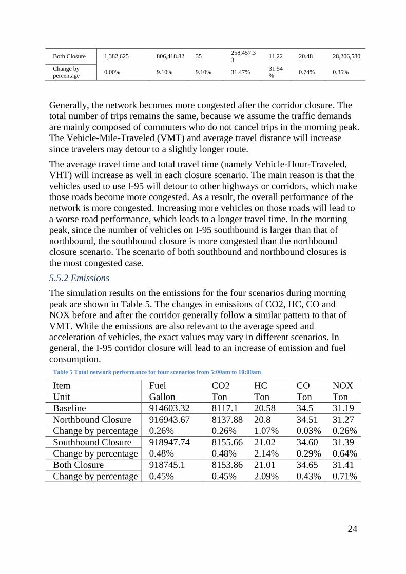
5.5.2 Emissions
The simulation results on the emissions for the four scenarios during morning
peak are shown in Table 5. The changes in emissions of CO2, HC, CO and
NOX before and after the corridor generally follow a similar pattern to that of
VMT. While the emissions are also relevant to the average speed and
acceleration of vehicles, the exact values may vary in different scenarios. In
general, the I-95 corridor closure will lead to an increase of emission and fuel
consumption.
Table 5 Total network performance for four scenarios from 5:00am to 10:00am
Item Fuel CO2 HC CO NOX
Unit Gallon Ton Ton Ton Ton
Baseline 914603.32 8117.1 20.58 34.5 31.19
Northbound Closure 916943.67 8137.88 20.8 34.51 31.27
Change by percentage 0.26% 0.26% 1.07% 0.03% 0.26%
Southbound Closure 918947.74 8155.66 21.02 34.60 31.39
Change by percentage 0.48% 0.48% 2.14% 0.29% 0.64%
Both Closure 918745.1 8153.86 21.01 34.65 31.41
Change by percentage 0.45% 0.45% 2.09% 0.43% 0.71%
25
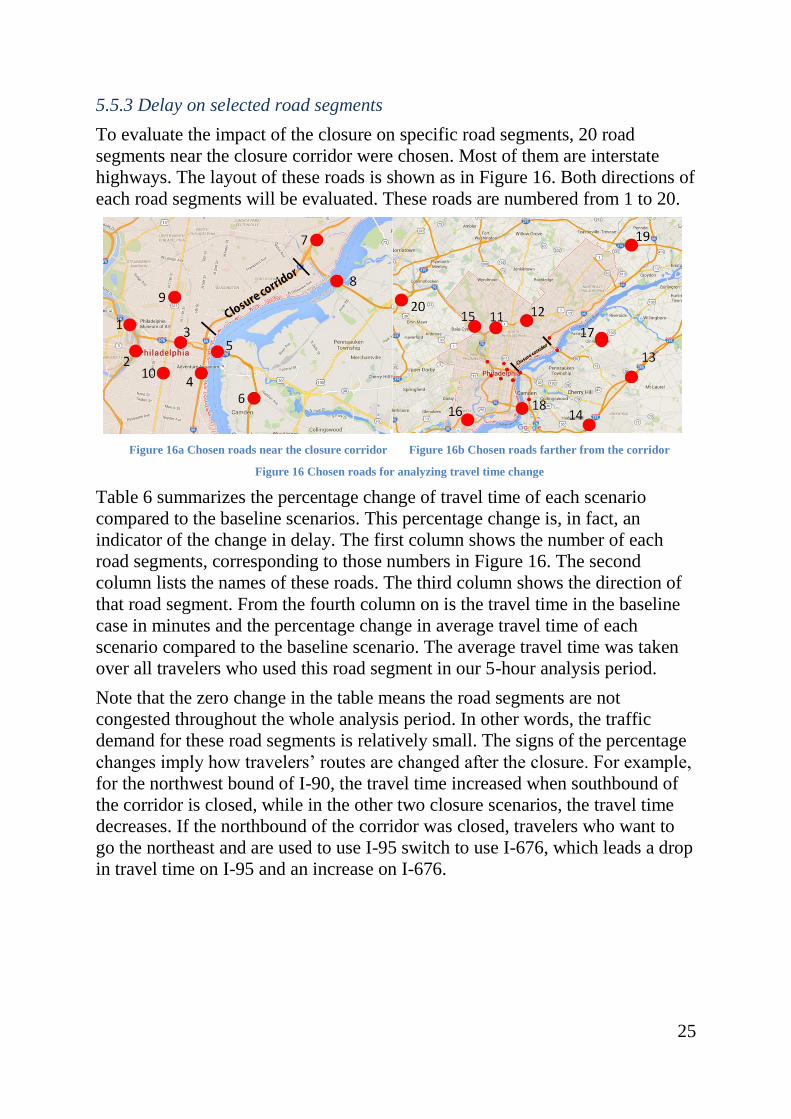
5.5.3 Delay on selected road segments
To evaluate the impact of the closure on specific road segments, 20 road
segments near the closure corridor were chosen. Most of them are interstate
highways. The layout of these roads is shown as in Figure 16. Both directions of
each road segments will be evaluated. These roads are numbered from 1 to 20.
Figure 16a Chosen roads near the closure corridor Figure 16b Chosen roads farther from the corridor
Figure 16 Chosen roads for analyzing travel time change
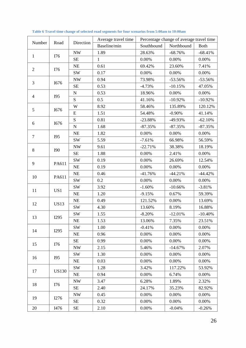
Table 6 summarizes the percentage change of travel time of each scenario
compared to the baseline scenarios. This percentage change is, in fact, an
indicator of the change in delay. The first column shows the number of each
road segments, corresponding to those numbers in Figure 16. The second
column lists the names of these roads. The third column shows the direction of
that road segment. From the fourth column on is the travel time in the baseline
case in minutes and the percentage change in average travel time of each
scenario compared to the baseline scenario. The average travel time was taken
over all travelers who used this road segment in our 5-hour analysis period.
Note that the zero change in the table means the road segments are not
congested throughout the whole analysis period. In other words, the traffic
demand for these road segments is relatively small. The signs of the percentage
changes imply how travelers’ routes are changed after the closure. For example,
for the northwest bound of I-90, the travel time increased when southbound of
the corridor is closed, while in the other two closure scenarios, the travel time
decreases. If the northbound of the corridor was closed, travelers who want to
go the northeast and are used to use I-95 switch to use I-676, which leads a drop
in travel time on I-95 and an increase on I-676.
26
Table 6 Travel time change of selected road segments for four scenarios from 5:00am to 10:00am
Number Road Direction Average travel time Percentage change of average travel time
Baseline/min Southbound Northbound Both
1 I76 NW 1.89 28.63% -68.76% -68.41%
SE 1 0.00% 0.00% 0.00%
2 I76 NE 0.61 69.42% 23.60% 7.41%
SW 0.17 0.00% 0.00% 0.00%
3 I676 NW 0.94 73.98% -53.56% -53.56%
SE 0.53 -4.73% -10.15% 47.05%
4 I95 N 0.53 18.96% 0.00% 0.00%
S 0.5 41.16% -10.92% -10.92%
5 I676 W 8.92 58.46% 135.89% 120.12%
E 1.51 54.48% -0.90% 41.14%
6 I676 S 0.81 -23.88% -49.93% -62.10%
N 1.68 -87.35% -87.35% -87.35%
7 I95 NE 1.82 0.00% 0.00% 0.00%
SW 5.59 -7.61% 66.98% 56.59%
8 I90 NW 9.61 -22.71% 38.38% 18.19%
SE 1.88 0.00% 2.41% 0.00%
9 PA611 SW 0.19 0.00% 26.69% 12.54%
NE 0.19 0.00% 0.00% 0.00%
10 PA611 NE 0.46 -41.76% -44.21% -44.42%
SW 0.2 0.00% 0.00% 0.00%
11 US1 SW 3.92 -1.60% -10.66% -3.81%
NE 1.20 -9.15% 0.67% 59.39%
12 US13 NE 0.49 121.52% 0.00% 13.69%
SW 4.30 13.60% 8.19% 16.88%
13 I295 SW 1.55 -8.20% -12.01% -10.40%
NE 1.53 13.06% 7.35% 23.51%
14 I295 SW 1.00 -0.41% 0.00% 0.00%
NE 0.96 0.00% 0.00% 0.00%
15 I76 SE 0.99 0.00% 0.00% 0.00%
NW 2.15 5.46% -14.67% 2.07%
16 I95 SW 1.30 0.00% 0.00% 0.00%
NE 0.03 0.00% 0.00% 0.00%
17 US130 SW 1.28 3.42% 117.22% 53.92%
NE 0.94 0.00% 6.74% 0.00%
18 I76 NW 3.47 6.28% 1.89% 2.32%
SE 2.40 24.17% 35.23% 82.92%
19 I276 NW 0.45 0.00% 0.00% 0.00%
SE 0.32 0.00% 0.00% 0.00%
20 I476 SE 2.10 0.00% -0.04% -0.26%
27
NW 2.09 0.00% 4.85% 0.00%
We see that I-76 Southbound (Road segment No. 1 and No. 2) was not impacted
by the closure. Northbound of road segment No. 9 (part of PA611) and
southbound of road No.10 (part of PA611) were not affected much either.
The road segment that is impacted most is the westbound of I-676 (road
segment No.5). Due to the I-95 closure, travelers who drive to downtown from
the north and are used to use I-95 now need to detour through I-676. Those
travelers may also switch to I-76 (Road segment No.18) for detours, which
increased its travel time as well.
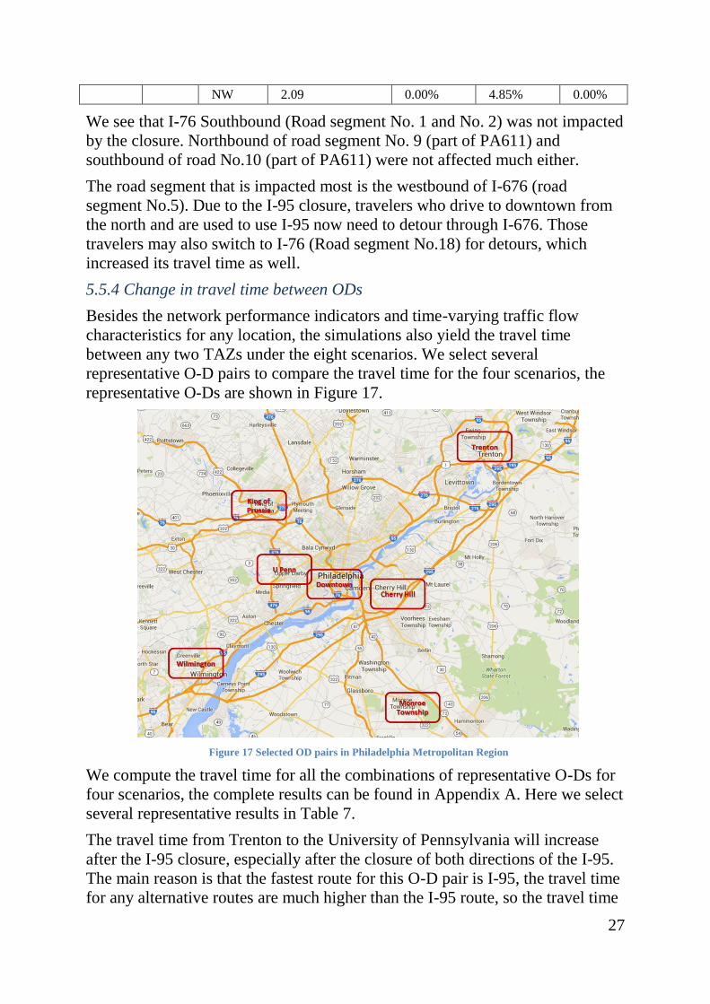
5.5.4 Change in travel time between ODs
Besides the network performance indicators and time-varying traffic flow
characteristics for any location, the simulations also yield the travel time
between any two TAZs under the eight scenarios. We select several
representative O-D pairs to compare the travel time for the four scenarios, the
representative O-Ds are shown in Figure 17.
Figure 17 Selected OD pairs in Philadelphia Metropolitan Region
We compute the travel time for all the combinations of representative O-Ds for
four scenarios, the complete results can be found in Appendix A. Here we select
several representative results in Table 7.
The travel time from Trenton to the University of Pennsylvania will increase
after the I-95 closure, especially after the closure of both directions of the I-95.
The main reason is that the fastest route for this O-D pair is I-95, the travel time
for any alternative routes are much higher than the I-95 route, so the travel time
28
after the closure will significantly increase. For the travel time from Wilmington
to Philadelphia downtown, since the original route does not contain the I-95
corridor, the travel time will not change as much after the closure.
The result on the travel time from the University of Pennsylvania to Wilmington
is quite interesting. During 7:00am to 8:00am, the travel time is getting slightly
worse since the closure will make the network more congested in general, so the
route between this O-D pair is also affected. However, during 8:00am to 9:00am,
since the north part of I-95 is closed, there are fewer vehicles in the south part
of I-95 (both directions). The fastest route contains the south part of I-95, and
thus it will be smoother to drive on the south part of I-95, resulting in a less
travel time.
Table 7 Travel time change of selected ODs for four scenarios from 5:00am to 10:00am (minutes)
Origin Destination Time
Interval
Base
line
I-95 south
closure
I-95 north
closure
I-95 both
closure
Trenton University of
Pennsylvania
7:00 -
8:00 44.9 44.9 49.4 53.1
Trenton University of
Pennsylvania
8:00 -
9:00 45.6 47.3 53.3 53.9
Wilmington Philadelphia
Downtown
7:00 -
8:00 31.9 31.9 31.9 31.9
Wilmington Philadelphia
Downtown
8:00 -
9:00 31.9 32.9 31.9 31.9
University of
Pennsylvania Wilmington
7:00 -
8:00 34.2 34.2 32.2 33.1
University of
Pennsylvania Wilmington
8:00 -
9:00 34.5 34.5 32.2 32.2
5.6 Afternoon peak network performance
5.6.1 Overall performance
Figure 18 Simulation profile for morning peak baseline
29
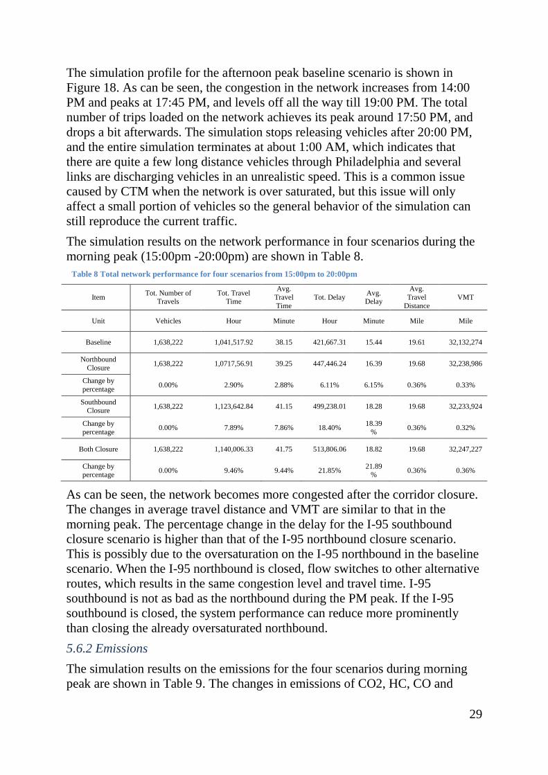
The simulation profile for the afternoon peak baseline scenario is shown in
Figure 18. As can be seen, the congestion in the network increases from 14:00
PM and peaks at 17:45 PM, and levels off all the way till 19:00 PM. The total
number of trips loaded on the network achieves its peak around 17:50 PM, and
drops a bit afterwards. The simulation stops releasing vehicles after 20:00 PM,
and the entire simulation terminates at about 1:00 AM, which indicates that
there are quite a few long distance vehicles through Philadelphia and several
links are discharging vehicles in an unrealistic speed. This is a common issue
caused by CTM when the network is over saturated, but this issue will only
affect a small portion of vehicles so the general behavior of the simulation can
still reproduce the current traffic.
The simulation results on the network performance in four scenarios during the
morning peak (15:00pm -20:00pm) are shown in Table 8.
Table 8 Total network performance for four scenarios from 15:00pm to 20:00pm
Item Tot. Number of
Travels Tot. Travel
Time
Avg.
Travel
Time
Tot. Delay Avg. Delay
Avg.
Travel
Distance
VMT
Unit Vehicles Hour Minute Hour Minute Mile Mile
Baseline 1,638,222 1,041,517.92 38.15 421,667.31 15.44 19.61 32,132,274
Northbound
Closure 1,638,222 1,0717,56.91 39.25 447,446.24 16.39 19.68 32,238,986
Change by
percentage 0.00% 2.90% 2.88% 6.11% 6.15% 0.36% 0.33%
Southbound Closure
1,638,222 1,123,642.84 41.15 499,238.01 18.28 19.68 32,233,924
Change by
percentage 0.00% 7.89% 7.86% 18.40%
18.39
% 0.36% 0.32%
Both Closure 1,638,222 1,140,006.33 41.75 513,806.06 18.82 19.68 32,247,227
Change by percentage
0.00% 9.46% 9.44% 21.85% 21.89
% 0.36% 0.36%
As can be seen, the network becomes more congested after the corridor closure.
The changes in average travel distance and VMT are similar to that in the
morning peak. The percentage change in the delay for the I-95 southbound
closure scenario is higher than that of the I-95 northbound closure scenario.
This is possibly due to the oversaturation on the I-95 northbound in the baseline
scenario. When the I-95 northbound is closed, flow switches to other alternative
routes, which results in the same congestion level and travel time. I-95
southbound is not as bad as the northbound during the PM peak. If the I-95
southbound is closed, the system performance can reduce more prominently
than closing the already oversaturated northbound.
5.6.2 Emissions
The simulation results on the emissions for the four scenarios during morning
peak are shown in Table 9. The changes in emissions of CO2, HC, CO and
30
NOX before and after the corridor generally follow a similar pattern to that of in
AM peak.
Table 9 Total network performance for four scenarios from 15:00pm to 20:00pm
Item Fuel CO2 HC CO NOX
Unit Gallon Ton Ton Ton Ton
Baseline 1047483.49 9296.42 23.82 39.55 35.8
Northbound Closure 1051571.08 9332.69 24.14 39.63 35.96
Change by percentage 0.39% 0.39% 1.34% 0.20% 0.45%
Southbound Closure 1052208.63 9338.35 24.33 39.63 36.01
Change by percentage 0.45% 0.45% 2.14% 0.20% 0.59%
Both Closure 1053393.72 9348.87 24.54 39.7 36.11
Change by percentage 0.56% 0.56% 3.02% 0.38% 0.87%
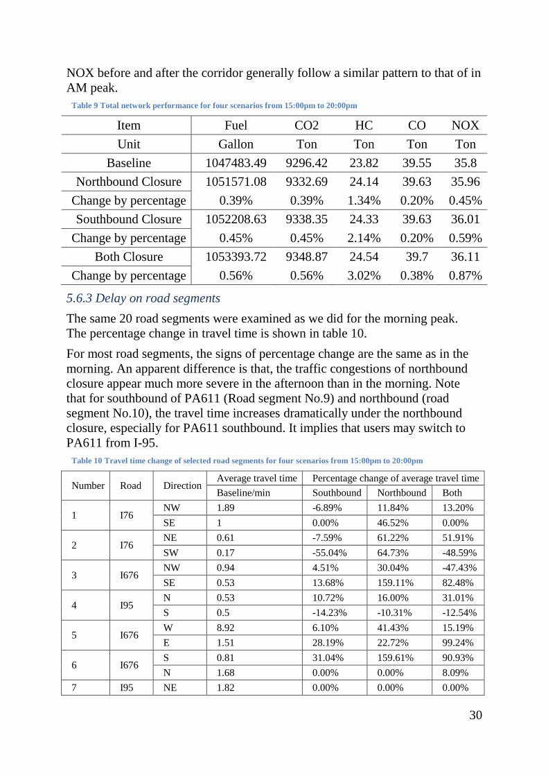
5.6.3 Delay on road segments
The same 20 road segments were examined as we did for the morning peak.
The percentage change in travel time is shown in table 10.
For most road segments, the signs of percentage change are the same as in the
morning. An apparent difference is that, the traffic congestions of northbound
closure appear much more severe in the afternoon than in the morning. Note
that for southbound of PA611 (Road segment No.9) and northbound (road
segment No.10), the travel time increases dramatically under the northbound
closure, especially for PA611 southbound. It implies that users may switch to
PA611 from I-95.
Table 10 Travel time change of selected road segments for four scenarios from 15:00pm to 20:00pm
Number Road Direction Average travel time Percentage change of average travel time
Baseline/min Southbound Northbound Both
1 I76 NW 1.89 -6.89% 11.84% 13.20%
SE 1 0.00% 46.52% 0.00%
2 I76 NE 0.61 -7.59% 61.22% 51.91%
SW 0.17 -55.04% 64.73% -48.59%
3 I676 NW 0.94 4.51% 30.04% -47.43%
SE 0.53 13.68% 159.11% 82.48%
4 I95 N 0.53 10.72% 16.00% 31.01%
S 0.5 -14.23% -10.31% -12.54%
5 I676 W 8.92 6.10% 41.43% 15.19%
E 1.51 28.19% 22.72% 99.24%
6 I676 S 0.81 31.04% 159.61% 90.93%
N 1.68 0.00% 0.00% 8.09%
7 I95 NE 1.82 0.00% 0.00% 0.00%
31
SW 5.59 82.10% 5.13% 84.97%
8 I90 NW 9.61 63.27% 15.87% 53.81%
SE 1.88 1.84% 0.00% 0.00%
9 PA611 SW 0.19 22.06% 196.61% 66.27%
NE 0.19 0.00% 0.00% 50.04%
10 PA611 NE 0.46 -17.68% 103.56% 1.64%
SW 0.2 0.00% 5.69% 28.49%
11 US1 SW 16.90 -1.60% -21.91% -16.62%
NE 2.09 -9.15% 128.26% 246.52%
12 US13 NE 0.49 121.52% 93.39% 158.16%
SW 13.80 13.60% -31.73% -2.45%
13 I295 SW 3.46 -8.20% 10.57% -2.55%
NE 3.16 13.06% -2.49% -42.55%
14 I295 SW 1.00 -0.41% 5.66% 7.30%
NE 0.96 0.00% 0.00% 0.00%
15 I76 SE 0.99 0.00% 197.27% 225.33%
NW 4.00 5.46% -5.88% -3.76%
16 I95 SW 1.30 0.00% 0.00% 0.00%
NE 1.50 0.00% 0.00% 0.00%
17 US130 SW 1.29 3.42% -1.35% 16.63%
NE 0.94 0.00% 0.00% 0.00%
18 I76 NW 7.37 6.28% 17.54% 19.41%
SE 3.72 24.17% 34.14% 98.66%
19 I276 NW 0.45 0.00% 0.00% 0.00%
SE 0.32 0.00% 0.00% 0.00%
20 I476 SE 2.10 0.00% 0.00% 0.00%
NW 2.09 0.00% 0.00% 0.00%
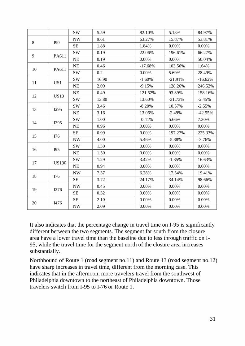
It also indicates that the percentage change in travel time on I-95 is significantly
different between the two segments. The segment far south from the closure
area have a lower travel time than the baseline due to less through traffic on I-
95, while the travel time for the segment north of the closure area increases
substantially.
Northbound of Route 1 (road segment no.11) and Route 13 (road segment no.12)
have sharp increases in travel time, different from the morning case. This
indicates that in the afternoon, more travelers travel from the southwest of
Philadelphia downtown to the northeast of Philadelphia downtown. Those
travelers switch from I-95 to I-76 or Route 1.
32
5.6.4 Change of travel time between O-Ds
We also computed the travel time for all the combinations of representative O-
Ds in Figure 12 for four scenarios during the PM peak, the complete results can
be found in Appendix B.
The general findings for the travel time change is that: if the chosen route before
I-95 closure contains I-95, then the travel time for that O-D pair will
significantly increase after the closure unless there exist alternative detour
routes that are comparable to I-95. For those O-D pairs that do not contain I-95
but are along the detour routes of I-95, then their travel time is slightly
influenced by the closure. For those travelers along the O-D pairs located on the
south of I-95, the closure may even benefit them due to the reduced volume on
I-95 south of downtown.
5.7 Conclusions
In off-line DTA modeling of this project, we conducted a dynamic network
analysis for Philadelphia Metropolitan Area and studied the traffic impact of the
I-95 corridor closure for both morning and afternoon peaks.
We utilize the network description files provided by DVPRC, archived traffic
flow data by PennDOT and DVPRC, and traffic speed data from INRIX to
validate the off-line dynamic traffic assignment model. We use the calibrated
model to predict and evaluate the traffic impact of I-95 corridor closures.
System performance, traffic delay on critical road segments and travel time
between selected O-Ds are compared and analyzed, which help better
understand the network conditions with and without I-95 closures.
In this part, we only calibrated the baseline scenario and predict the traffic
conditions for different I-95 closure scenarios for both AM and PM peaks, but
no management and operational strategies are made to reduce the traffic
congestion caused by the I-95 closure. In next section, we will design a
methodology to simulate the traffic on the real time basis. An on-site detour
strategy through Dynamic Message Signs (DMS) will be proposed to suggest
efficient detour routes, optimal traffic diversion ratios and text displays for
DMS.
33
6. Real-time DTA for Philadelphia Metropolitan Region
In this section we develop a regional dynamic network model that simulates
millions of trips in the Philadelphia metropolitan region and captures those
travelers’ travel behavior on real-time basis. It can be applied directly to predict
traffic impact of planned and unplanned incidents, and provide real-time
decision making for traffic operations.
The model takes incident reports and traffic speeds as real-time data feeds, and
O-D demands as the historical data feeds. The management strategy is adjusted
in the real time to achieve overall best performance for the entire network. The
model contains a closed-loop feedback learning mechanism, the
estimation/prediction accuracy will improve as the model runs.
In the case study, the model is developed to control all the dynamic message
signs (DMS) on I-95 corridor. On-site detour strategies through DMS will be
proposed to suggest efficient detour routes, optimal traffic diversion ratios and
texts for DMS. The real-time optimal compliance rates for each detour route can
be updated as time progresses by analyzing real-time traffic data (INRIX and/or
counts) and provided to PennDOT Transportation Management Center on the
real-time basis.
The model is implemented as an internet web application, a website built to
visualize the control strategies and animate the flow evolutions. All the user
interactions with the real-time traffic management model are based on browser.
6.1 Network settings
In this section we discuss the preparations especially for building the real-time
traffic management framework.
6.1.1 Dynamic network loading
Dynamic network loading (DNL) model is an essential component in real-time
DTA model. DNL models take time-dependent O-D demand and travelers'
behavior parameters as input and simulate the network conditions with a high
spatial-temporal resolution. The traffic flow, travel time of every links and
trajectory of every vehicle can be recorded during the simulation. We denote the
simulation process as:
St+1 = DNL(q, p, St)
Where St is the traffic state of the whole network on time t, q is the O-D
demand vector and p is the route choice probability of each route. After the
DNL for one interval, we have the network condition on time t + 1, denoted as
St+1.
Two major components in DNL models are link flow evolution models and
node flow evolution models. The link flow evolution models describe the
34
dynamic relationship between vehicle density, speed and volume for one road
segment. Cell transmission model (CTM), as a finite element approximation to
the partial differential equation of fluid evolution, is proved to best simulate the
flow propagation on road segments. This project adopts CTM to simulate the
flow propagation on links. Node flow evolution models depict the traffic flow
propagation (merge and diverge) on junctions. A simple node model (Jin &
Zhang 2003) that satisfies the “fairness” condition is adopted. The adopted
node model is proved to have high-throughput and is computationally efficient.
The DNL model is implemented under C++. The dependency management is
due to CMake.
6.1.2 Real-time traffic speed measurements
Traffic speed data were obtained from INRIX4. The traffic speed data is
provided at the geographic level of Traffic Message Channel (TMC), one of the
geo-reference protocols. To match the TMC units with links in the road network,
an algorithm considering relative distance and direction was developed to
search for the best match for each TMC.
Traffic speed data cover most of the corridors and major roads in Philadelphia
Metropolitan Region. The data set includes 13,104 TMCs for the nine counties
of DVRPC. The data includes speed, travel time, historic average speed and
reference speed (namely 85% quantile of all observed probe vehicle speeds,
used as the free-flow speed).
INRIX provides an API to let users request the real-time traffic speed data feeds
nation-wide. We implemented a crawler to continuously retrieves, processes,
summarizes the real-time traffic speed and reports the results to the traffic
management server.
6.1.3 Path set generation
The paths for each O-D pair are pre-determined before the real-time traffic
management. To generate paths for one O-D pair, we execute the shortest path
algorithm from origin to destination under different traffic conditions: light,
heavy and congested. The path set contains paths for all different pairs of O-D.
For DVPRC network, totally 189,065 paths are generated for 473,796 O-D pairs.
6.2 DMS based real-time network flow model
In this section we present the proposed real-time traffic management model. We
first overview its structure and define each component in the model, then we
formulate and interpret each component separately. The solution algorithm to
each proposed component is also provided.
4 INRIX, http://www.inrix.com
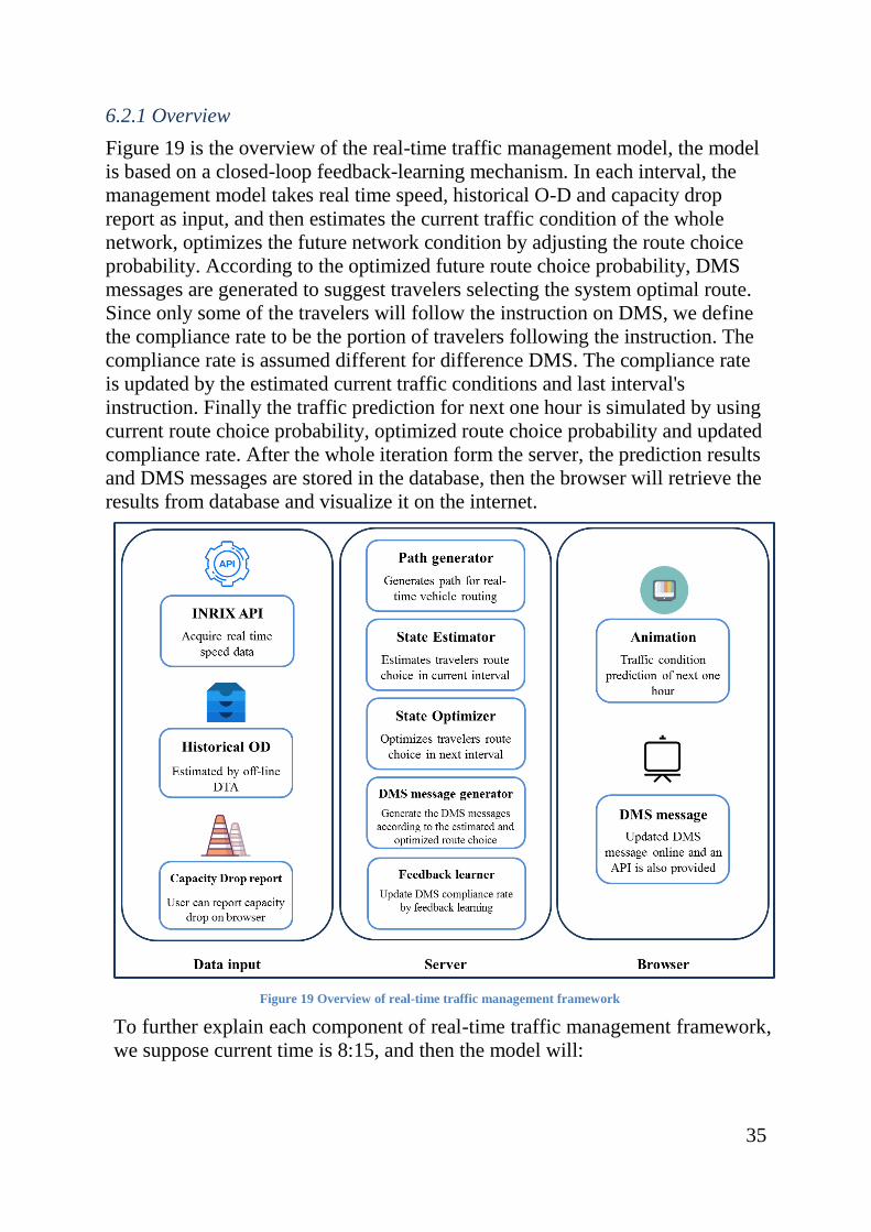
35
6.2.1 Overview
Figure 19 is the overview of the real-time traffic management model, the model
is based on a closed-loop feedback-learning mechanism. In each interval, the
management model takes real time speed, historical O-D and capacity drop
report as input, and then estimates the current traffic condition of the whole
network, optimizes the future network condition by adjusting the route choice
probability. According to the optimized future route choice probability, DMS
messages are generated to suggest travelers selecting the system optimal route.
Since only some of the travelers will follow the instruction on DMS, we define
the compliance rate to be the portion of travelers following the instruction. The
compliance rate is assumed different for difference DMS. The compliance rate
is updated by the estimated current traffic conditions and last interval's
instruction. Finally the traffic prediction for next one hour is simulated by using
current route choice probability, optimized route choice probability and updated
compliance rate. After the whole iteration form the server, the prediction results
and DMS messages are stored in the database, then the browser will retrieve the
results from database and visualize it on the internet.
Figure 19 Overview of real-time traffic management framework
To further explain each component of real-time traffic management framework,
we suppose current time is 8:15, and then the model will:
36
Acquire data: acquire the real-time traffic speed and incident reports in
[8:00, 8:15]
Estimate Previous: estimate the route choice probability in [8:00, 8:15]
Compliance rate update: update the DMS compliance rate calculated in
[7:45, 8:00]
Optimize Next interval: optimize the route choice probability in [8:15,
8:30]
Generate DMS Message: based on the optimized and estimated route
choice, generate DMS message for [8:15, 8:30]
Predict Future: Predict traffic state in next one hour using updated
compliance rate
Next interval: Wait until current time is 8:30, go back to acquire data
In the following sections, we discuss each component in detail, we
assume the current interval is t + 1.
6.2.2 Traffic state estimation for the current stage
In the current traffic state estimation component, we want to find the current
travelers' route choice probability that makes DNL model better reproduce the
observed traffic speed. So the formulation is to minimize the errors between
observed traffic speed tao and simulated traffic speed ta. ta is obtained from the
simulated network condition St+1, the function Ta(⋅) is the travel time retrieval
function to get travel time on link a from simulated network conditions. The
overall formulation for estimating current traffic state is as follows.
The first constraint in the formulation requires the sum of route choice
probability for one O-D pair is 1, r represents the origin, s represents destination
and k represents path. The second constraint requires all route choice
probabilities are non-negative. The third constraint indicates that the current
traffic condition St+1 is simulated from traffic state of last interval with demand
q and route choice probability. Different route choice probability will result in
different link travel time ta. The whole formulation searches for the best p
which approximates the observed link travel time tao best.
37
After solving the above formulation, the solved route choice probabilities
represent travelers' behavior in current interval. By running the DNL model
with route choice probability p and O-D demand q, current traffic conditions on
every link can be retrieved.
Since DNL(q, p, St) is a simulation process, which can't be analytically
decomposed, above formulation is a hard non-linear optimization problem.
Analytically calculating the derivative of the objective function is impossible,
the numerical derivative can still be calculated (Qian et al. 2012). Qian
proposed the method to numerically calculate the derivative of path flow, by
chain rule the derivative of route choice probability can also be obtained. The
chain rule is formulated as follows:
6.2.3 Traffic state optimization for future stages
In the sub-problem of optimizing future traffic state, we search for the best route
choice probability for all O-D pairs such that the total travel time in the whole
network is minimum. The optimization is formulated as follows:
The first two constraints are the same as those in the former formulation, the
third constraint indicates we use the estimated current state St+1 as input and
simulate the future interval St+2. Ta and Xa are link travel time and link flow
retrieval function, respectively. The formulation above searches for the best
route choice probability p such that the total network travel time on interval t+2
is minimized.
After solving the above formulation, the solved route choice probability
represents the best route choice probability for the next interval. However, since
we cannot directly control travelers' route choice, we can only use DMS
messages to suggest the best route for travelers. If the compliance rate is high,
the network approaches more to the system optimal.
38
Similar with former formulation, the numerical derivative of the objective
function can be calculated from the simulation (Qian et al. 2012). Though
objective function is different, the solution algorithm is almost the same.
6.2.4 Feedback learning of compliance rate
The feedback learning of compliance rate is based on the estimated route choice
calculated in interval t, detour instruction generated in interval t and estimated
route choice calculated in interval t+1. Both route choice probability represent
the estimated current traffic state, but the former is the results for interval t and
latter is the results for interval t+1. We denote the former as pt and latter as pt+1.
So the new compliance rate can be calculated by comparing pt, pt+1 and detour
link adetour. Define I(⋅) is an indicator function, the compliance rate for DMS d,
cd can be calculated as:
A method of successive averaging (MSA) mechanism can be adopted to update
the compliance rate in each interval.
According to the definition of compliance rate, it represents the portion of
travelers that follow the DMS instruction. If all travelers follow the instruction,
then prsk = 0 if adetour is not in path frs
k . The feedback learning sub-problem can
be done after the current state estimation sub-problem, it is independent with the
future traffic state optimization sub-problem.
6.2.5 DMS message generation
The generation of DMS message is based on the estimated route choice
probability pest and optimized route choice probabilitypopt. For link a, if the
optimized link flow is smaller than the estimated route flow, then it means some
travelers shouldn't take link a, therefore a detour is suggested.
Our model is based on such criterion to decide whether travelers are supposed
to take the detour on certain links. After calculated the detour link (or decide not
to detour), the message generation rule is as follows:
If the congestion is ahead and the travelers on the highways are
supposed to take the detour, the message will be “CONGESTION
AHEAD, XX MINUTES TO NEXT EXIT, TAKE NEXT EXIT”, paired
with a disclaimer message for traffic engineers, “if taking exits is
suggested, it should be paired with DMS on the arterials guiding
drivers”.
39
If the congestion is ahead but the travelers on the highways should still
take the highway, the message will be “CONGESTION AHEAD, XX
MINUTES TO NEXT EXIT”.
If there is no congestion ahead, the message will be “DRIVE WITH
CARE”.
The above rule is only for demonstration purpose, a detailed generation rule can
be easily extended from current framework. Note the DMS message generation
process is independent with feedback learning of compliance rate process, and
solving these two sub-problems can be in any order or not necessarily sequential.
Note if we display “CONGESTION AHEAD, XX MINUTES TO NEXT
EXIT”, we’re not suggesting a detour to travelers. We just provide the
information to let them choose whether to take next exit or not. However,
“CONGESTION AHEAD, TAKE NEXT EXIT” message is suggesting
travelers taking next exit.
This tool that generates optimal DMS can be fed to ATMS for displaying and
coordinating DMS. However, it also requires ATMS to set up proper messages
for DMS on those alternative detour routes. Alternative routes at certain
locations (or freeway exits) can be predetermined. When congestion is detected
and detour from freeway is suggested due to incidents, the ATMS can automate
the DMS texts on those predetermined alternative routes to guide travelers. This
tool will work best under the coordination with ATMS, which should be further
investigated.
6.2.6 Traffic states prediction for future stages
We predict the traffic conditions for the next hour, the prediction is based on the
DMS message, current traffic conditions and compliance rate. Since we have
already decided the DMS messages and also updated the compliance rate,
predicted route choice probability ppre can be calculated from current route
choice probability pest. Then by running the DNL model using the predicted
route choice probability ppre, traffic evolution for next one hour can be
calculated.
6.3 Browser-based implementation
In this section we present a browser-based implementation of the proposed real-
time traffic management model. On the back-end, a server keeps updating the
real-time traffic conditions and predicting the future traffic conditions, and on
the front-end users can visualize the DMS messages and the animation of
predicted network flow evolution through a web browser.
The web application can be visited using the following link:
http://bruno.heinz.cmu.edu/traffic/congestion_online/
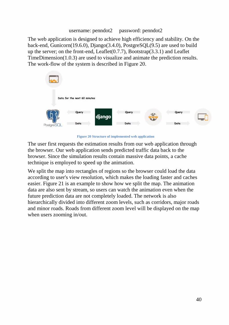
40
username: penndot2 password: penndot2
The web application is designed to achieve high efficiency and stability. On the
back-end, Gunicorn(19.6.0), Django(3.4.0), PostgreSQL(9.5) are used to build
up the server; on the front-end, Leaflet(0.7.7), Bootstrap(3.3.1) and Leaflet
TimeDimension(1.0.3) are used to visualize and animate the prediction results.
The work-flow of the system is described in Figure 20.
Figure 20 Structure of implemented web application
The user first requests the estimation results from our web application through
the browser. Our web application sends predicted traffic data back to the
browser. Since the simulation results contain massive data points, a cache
technique is employed to speed up the animation.
We split the map into rectangles of regions so the browser could load the data
according to user's view resolution, which makes the loading faster and caches
easier. Figure 21 is an example to show how we split the map. The animation
data are also sent by stream, so users can watch the animation even when the
future prediction data are not completely loaded. The network is also
hierarchically divided into different zoom levels, such as corridors, major roads
and minor roads. Roads from different zoom level will be displayed on the map
when users zooming in/out.
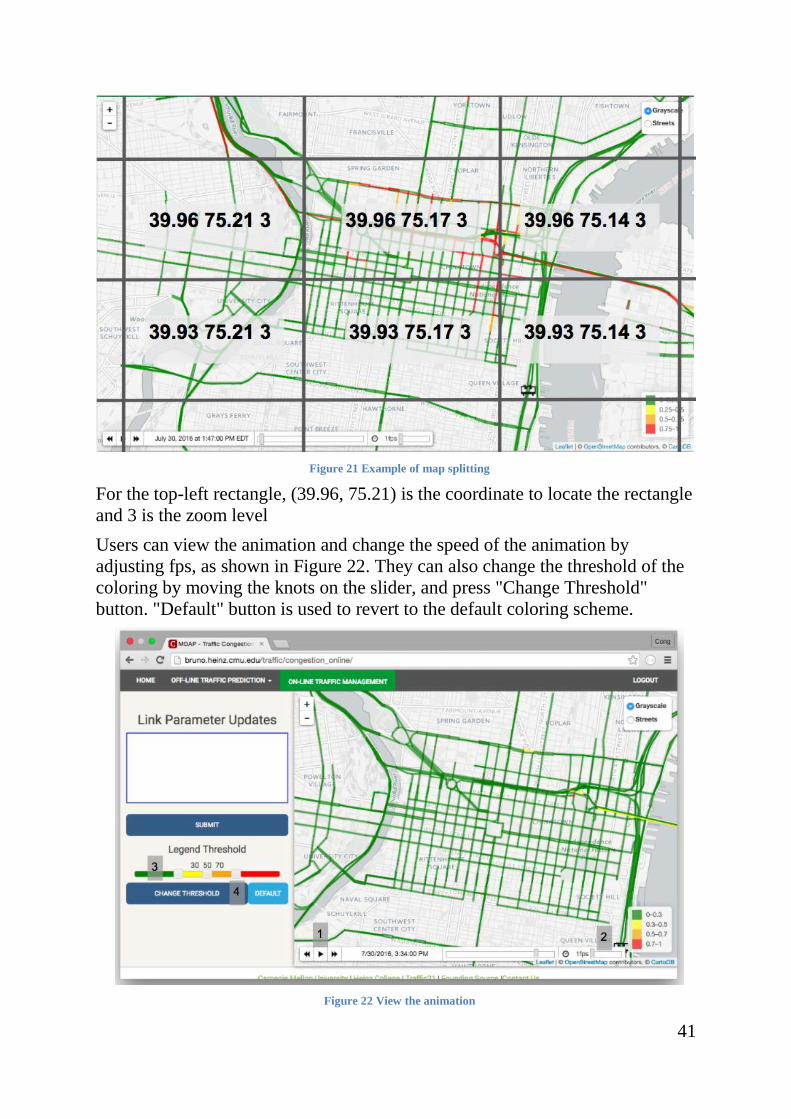
41
Figure 21 Example of map splitting
For the top-left rectangle, (39.96, 75.21) is the coordinate to locate the rectangle
and 3 is the zoom level
Users can view the animation and change the speed of the animation by
adjusting fps, as shown in Figure 22. They can also change the threshold of the
coloring by moving the knots on the slider, and press "Change Threshold"
button. "Default" button is used to revert to the default coloring scheme.
Figure 22 View the animation
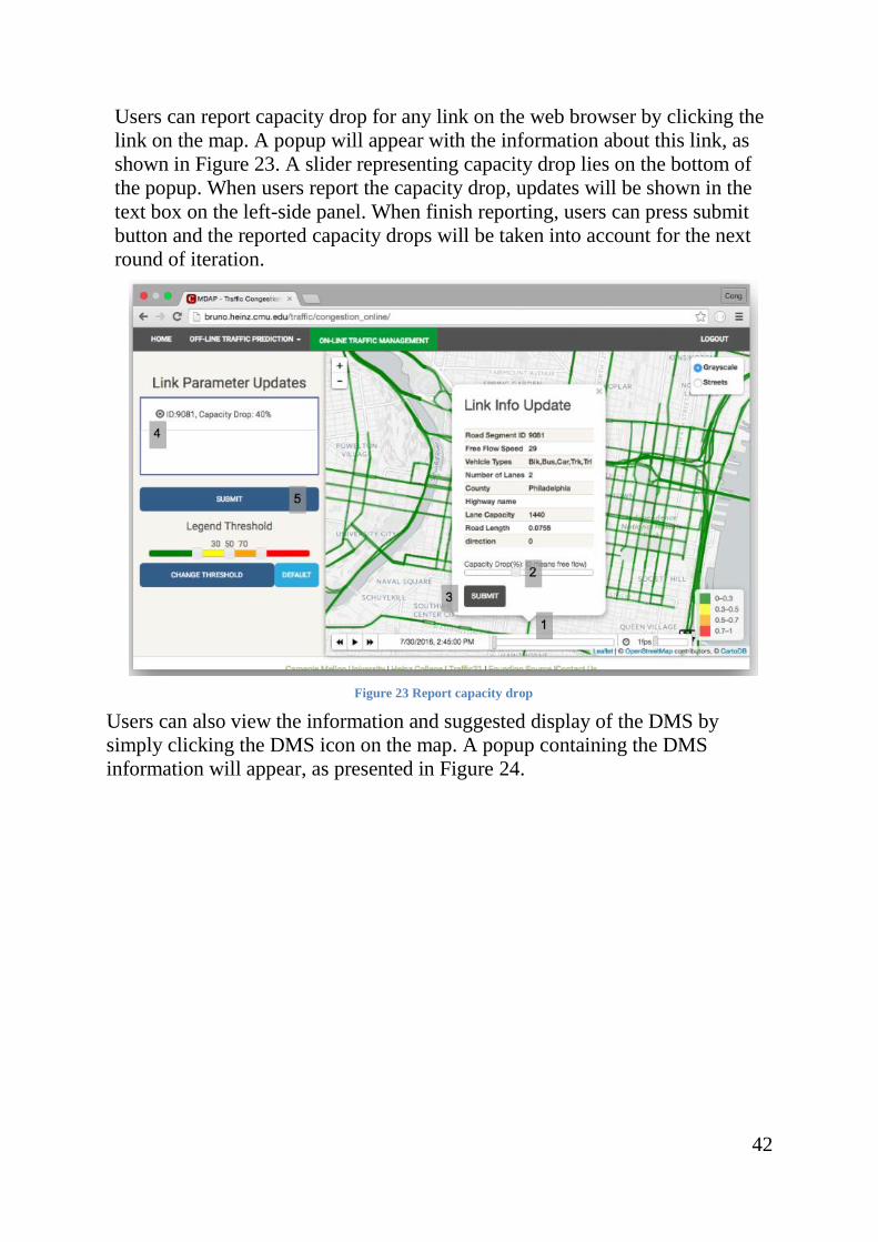
42
Users can report capacity drop for any link on the web browser by clicking the
link on the map. A popup will appear with the information about this link, as
shown in Figure 23. A slider representing capacity drop lies on the bottom of
the popup. When users report the capacity drop, updates will be shown in the
text box on the left-side panel. When finish reporting, users can press submit
button and the reported capacity drops will be taken into account for the next
round of iteration.
Figure 23 Report capacity drop
Users can also view the information and suggested display of the DMS by
simply clicking the DMS icon on the map. A popup containing the DMS
information will appear, as presented in Figure 24.
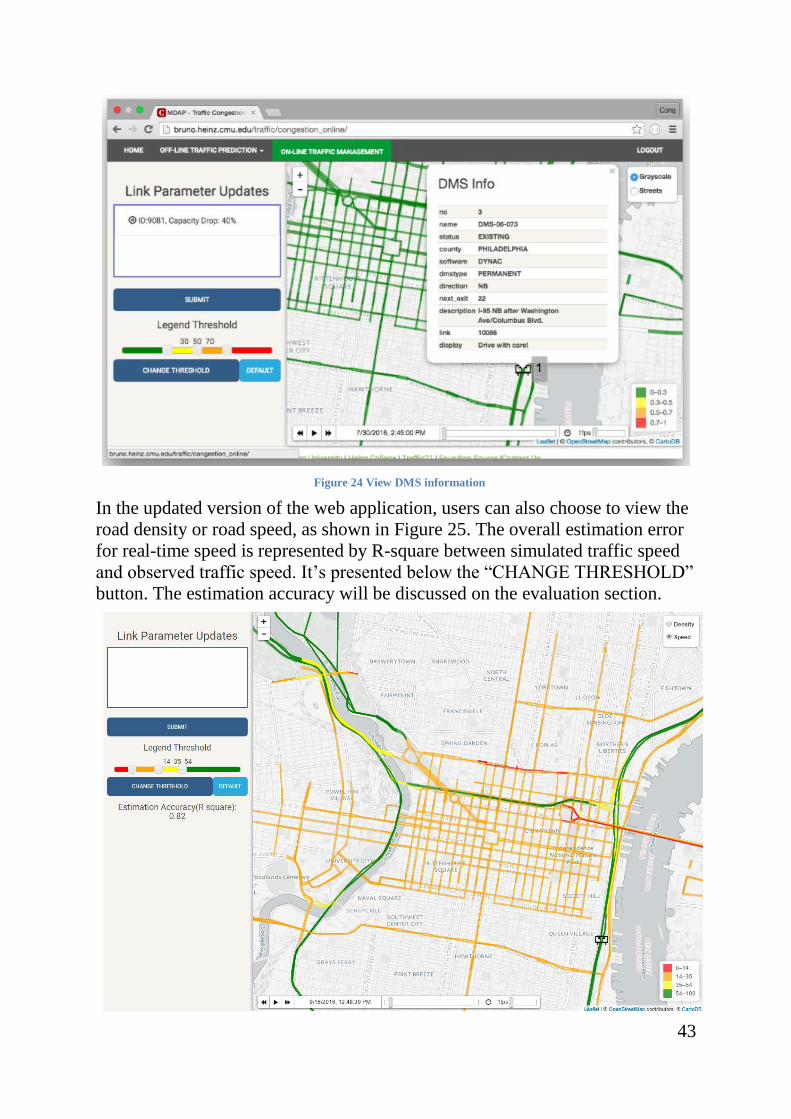
43
Figure 24 View DMS information
In the updated version of the web application, users can also choose to view the
road density or road speed, as shown in Figure 25. The overall estimation error
for real-time speed is represented by R-square between simulated traffic speed
and observed traffic speed. It’s presented below the “CHANGE THRESHOLD”
button. The estimation accuracy will be discussed on the evaluation section.
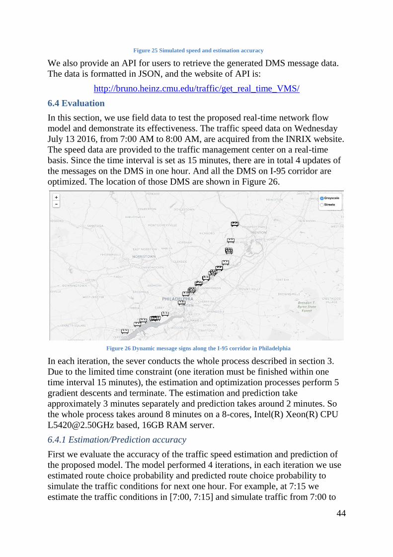
44
Figure 25 Simulated speed and estimation accuracy
We also provide an API for users to retrieve the generated DMS message data.
The data is formatted in JSON, and the website of API is:
http://bruno.heinz.cmu.edu/traffic/get_real_time_VMS/
6.4 Evaluation
In this section, we use field data to test the proposed real-time network flow
model and demonstrate its effectiveness. The traffic speed data on Wednesday
July 13 2016, from 7:00 AM to 8:00 AM, are acquired from the INRIX website.
The speed data are provided to the traffic management center on a real-time
basis. Since the time interval is set as 15 minutes, there are in total 4 updates of
the messages on the DMS in one hour. And all the DMS on I-95 corridor are
optimized. The location of those DMS are shown in Figure 26.
Figure 26 Dynamic message signs along the I-95 corridor in Philadelphia
In each iteration, the sever conducts the whole process described in section 3.
Due to the limited time constraint (one iteration must be finished within one
time interval 15 minutes), the estimation and optimization processes perform 5
gradient descents and terminate. The estimation and prediction take
approximately 3 minutes separately and prediction takes around 2 minutes. So
the whole process takes around 8 minutes on a 8-cores, Intel(R) Xeon(R) CPU
[email protected] based, 16GB RAM server.
6.4.1 Estimation/Prediction accuracy
First we evaluate the accuracy of the traffic speed estimation and prediction of
the proposed model. The model performed 4 iterations, in each iteration we use
estimated route choice probability and predicted route choice probability to
simulate the traffic conditions for next one hour. For example, at 7:15 we
estimate the traffic conditions in [7:00, 7:15] and simulate traffic from 7:00 to
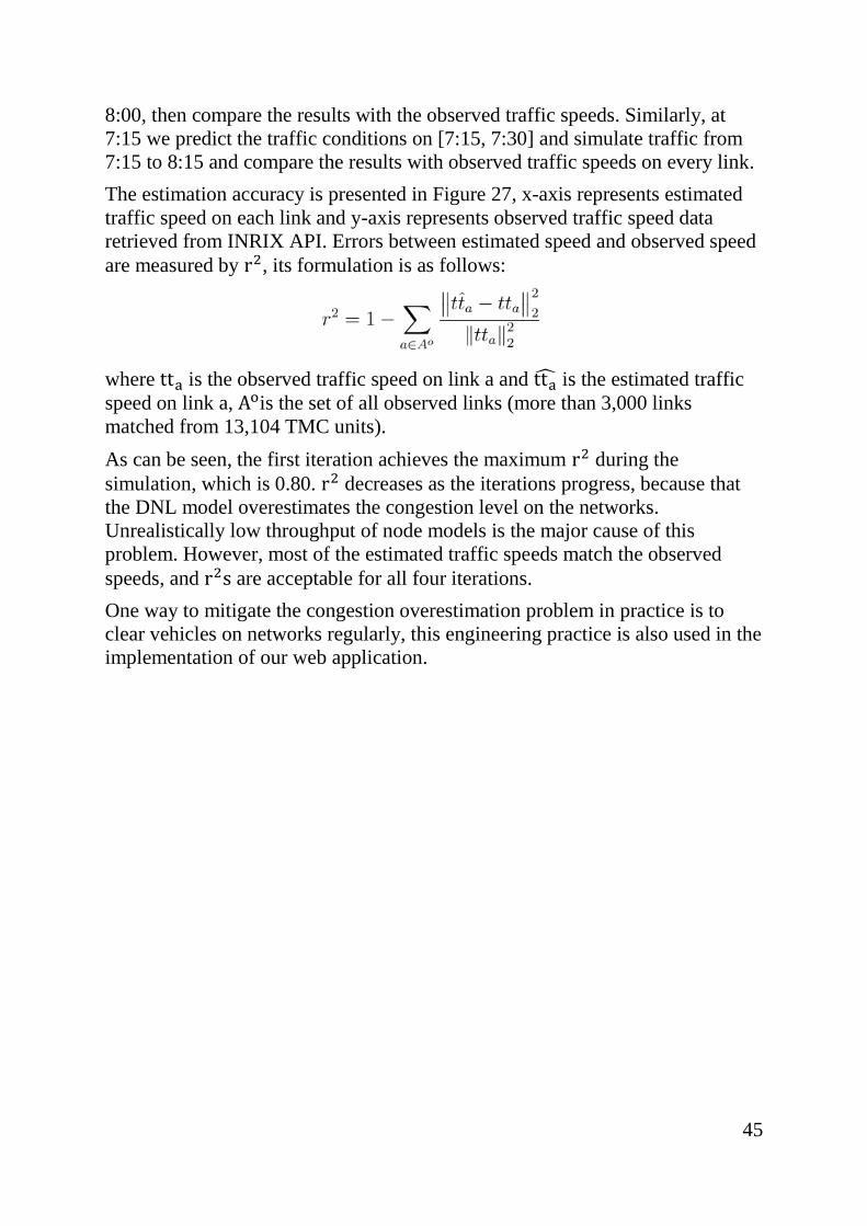
45
8:00, then compare the results with the observed traffic speeds. Similarly, at
7:15 we predict the traffic conditions on [7:15, 7:30] and simulate traffic from
7:15 to 8:15 and compare the results with observed traffic speeds on every link.
The estimation accuracy is presented in Figure 27, x-axis represents estimated
traffic speed on each link and y-axis represents observed traffic speed data
retrieved from INRIX API. Errors between estimated speed and observed speed
are measured by r2, its formulation is as follows:
where tta is the observed traffic speed on link a and tta is the estimated traffic
speed on link a, Aois the set of all observed links (more than 3,000 links
matched from 13,104 TMC units).
As can be seen, the first iteration achieves the maximum r2 during the
simulation, which is 0.80. r2 decreases as the iterations progress, because that
the DNL model overestimates the congestion level on the networks.
Unrealistically low throughput of node models is the major cause of this
problem. However, most of the estimated traffic speeds match the observed
speeds, and r2s are acceptable for all four iterations.
One way to mitigate the congestion overestimation problem in practice is to
clear vehicles on networks regularly, this engineering practice is also used in the
implementation of our web application.
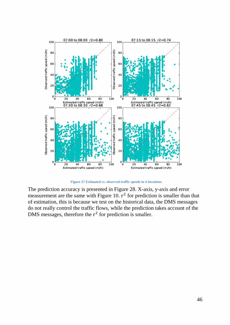
46
Figure 27 Estimated vs. observed traffic speeds in 4 iterations
The prediction accuracy is presented in Figure 28. X-axis, y-axis and error
measurement are the same with Figure 10. r2 for prediction is smaller than that
of estimation, this is because we test on the historical data, the DMS messages
do not really control the traffic flows, while the prediction takes account of the
DMS messages, therefore the r2 for prediction is smaller.
47
Figure 28 Predicted vs. observed traffic speeds in 4 iterations
6.4.2 Control effectiveness
To measure the impacts of DMS messages on the overall network performance,
we inspect the total travel time on every link, the total travel time on link a is
denoted as:
where Tota is the total travel time on link a, xa is the traffic flow on link a and
ta is the travel time on link a. The box plots for total travel time of all links on 4
iterations are shown in Figure 29 separately. As can be seen, the boxes for
different traffic conditions are on similar level, which indicates that the control
of DMS on I-95 has small influence on the overall network performance. This is
because the network we use is large so the controls on single corridor do not
have significant impacts on the overall network. However, the intervened traffic
still yields a lower total travel time. If we have more controls over the network
flow, the effectiveness of the control would be anticipated to increase.
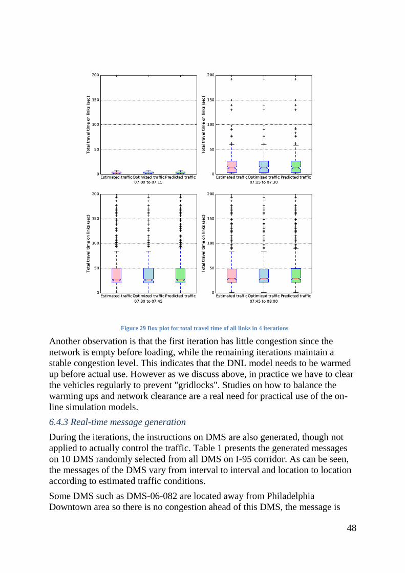
48
Figure 29 Box plot for total travel time of all links in 4 iterations
Another observation is that the first iteration has little congestion since the
network is empty before loading, while the remaining iterations maintain a
stable congestion level. This indicates that the DNL model needs to be warmed
up before actual use. However as we discuss above, in practice we have to clear
the vehicles regularly to prevent "gridlocks". Studies on how to balance the
warming ups and network clearance are a real need for practical use of the on-
line simulation models.
6.4.3 Real-time message generation
During the iterations, the instructions on DMS are also generated, though not
applied to actually control the traffic. Table 1 presents the generated messages
on 10 DMS randomly selected from all DMS on I-95 corridor. As can be seen,
the messages of the DMS vary from interval to interval and location to location
according to estimated traffic conditions.
Some DMS such as DMS-06-082 are located away from Philadelphia
Downtown area so there is no congestion ahead of this DMS, the message is
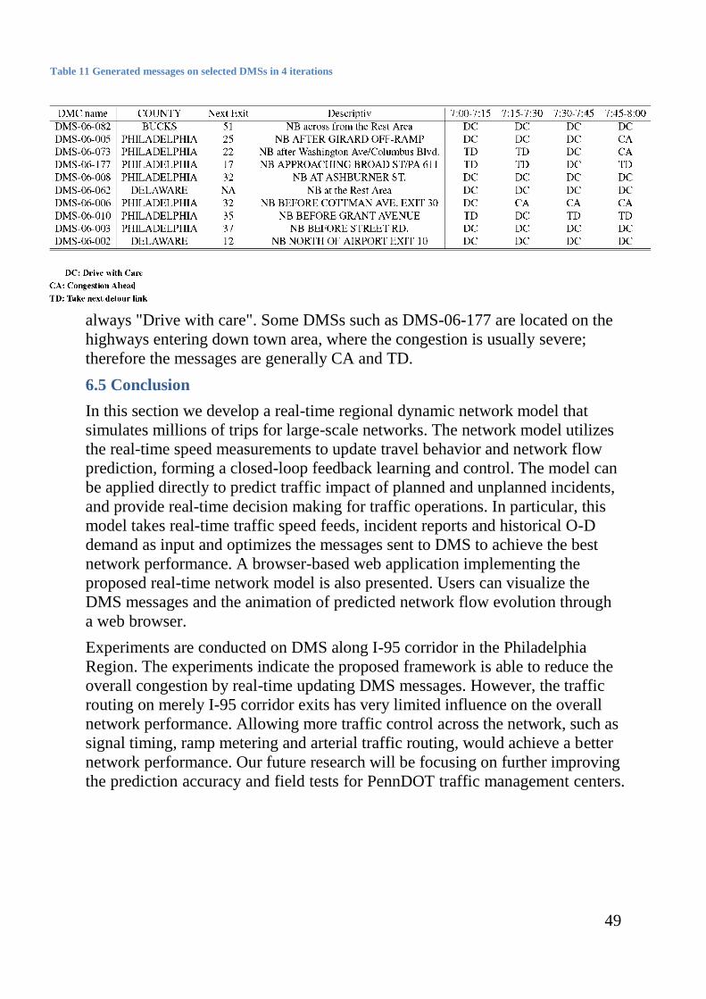
49
always "Drive with care". Some DMSs such as DMS-06-177 are located on the
highways entering down town area, where the congestion is usually severe;
therefore the messages are generally CA and TD.
6.5 Conclusion
In this section we develop a real-time regional dynamic network model that
simulates millions of trips for large-scale networks. The network model utilizes
the real-time speed measurements to update travel behavior and network flow
prediction, forming a closed-loop feedback learning and control. The model can
be applied directly to predict traffic impact of planned and unplanned incidents,
and provide real-time decision making for traffic operations. In particular, this
model takes real-time traffic speed feeds, incident reports and historical O-D
demand as input and optimizes the messages sent to DMS to achieve the best
network performance. A browser-based web application implementing the
proposed real-time network model is also presented. Users can visualize the
DMS messages and the animation of predicted network flow evolution through
a web browser.
Experiments are conducted on DMS along I-95 corridor in the Philadelphia
Region. The experiments indicate the proposed framework is able to reduce the
overall congestion by real-time updating DMS messages. However, the traffic
routing on merely I-95 corridor exits has very limited influence on the overall
network performance. Allowing more traffic control across the network, such as
signal timing, ramp metering and arterial traffic routing, would achieve a better
network performance. Our future research will be focusing on further improving
the prediction accuracy and field tests for PennDOT traffic management centers.
Table 11 Generated messages on selected DMSs in 4 iterations
50
7. Discussions
In this section we present how our models can be tied with ATMS model and
what are the limitations of the propose model.
7.1 Extension with ATMS
In the proposed method, we pre-determine the detour route before the real-time
control. Our method evaluates the congestion level of detour route and optimal
route on the real-time basis and provides suggestions to travelers through DMS.
With ATMS, the detour route at certain locations can be determined on a real-
time basis. For example, when congestion is detected due to incidents on certain
road, the ATMS can automate our model not to select that road, and generate
texts to divert people on those alternative routes (e.g., Exit X, take street A).
Also, since the control is based on DMS message, only aggregated control can
be applied on I-95 corridor. Travelers to different destination receive the same
control message, control on individuals is impossible. But if our model is tied
with ATMS, the model can be tailored to provide different suggestion for
travelers with different destinations.
Besides, ATMS can also be an input to our proposed model. For example,
weather information, accident information and major events have significant
impact to the prediction accuracy. If ATMS can provide such information to our
real-time control model, the control policy is expected to be more precise.
7.2 Limitation of the proposed model
One major limitation of the proposed model is due to the restricted performance
of the estimation/optimization algorithms through entire road networks.
Although state-of-art algorithm is employed in this project, the convergence of
the estimation/optimization algorithm is still not guaranteed. The main reason
for the limited performance on network results from the convoluted relationship
between network variables.
Another limitation is due to the computational complexity of the traffic
simulation process. To achieve an accurate simulation result, more
computational time is usually required for the model. Since our model runs on a
real-time basis, the computational time is strictly constrained. In the future
extension, multi-thread/process algorithm can be developed to enhance the
simulation accuracy.
51
8. Summary
This project developed a general regional network model to estimate/predict
time-varying traffic evolution on all highways and major arterials in
Philadelphia Metropolitan Region. A case study was conducted for Center City
bridge closures: assess the dynamic traffic impact of Center City bridge closures
on both freeways and major arterials in the Philadelphia Region; propose real-
time traffic detour plans as a way of using travel demand management (TDM)
strategies to mitigate overall impact caused by closures.
We first collect data we need for the project and summarize the data. Then we
focus on establishing a dynamic network model for the Philadelphia
Metropolitan Region. A dynamic transportation network model that provides
estimated day-to-day origin-destination demand among all Traffic Analysis
Zones (TAZs) is developed. We examine and carefully calibrate the route
choices for all the travelers with different origins and destinations using
observed traffic counts and speed data. The calibrated model is capable of
estimating network-wide traffic impact caused by any incident based upon a
generic regional network consisting of freeway and major arterials.
We also developed a real-time DTA algorithm that take real-time incident
reports and real-time speed measurements simultaneously to update the
underlying flow propagation. In addition to predicting next-hour network flow,
we intend to intervene the network flow by optimizing the messages fed to
dynamic message signs (DMS). Real-time DTA is essentially solved with, in
part, optimal traffic routing only at limited DMS locations. The real-time
prediction and message optimum are solved with algorithms that are
computationally efficient for large-scale network.
This project contributes to the methodology foundation of a real-time traffic
control system in three aspects. First, we develop real-time DTA algorithms that
take real-time incident reports and real-time speed measurements
simultaneously to update the underlying flow propagation. Second, in addition
to predicting next-hour network flow, we intend to intervene the network flow
by optimizing the messages fed to dynamic message signs (DMS). Real-time
DTA is essentially solved with, in part, optimal traffic routing only at limited
DMS locations. Third, the real-time prediction and message optimum are solved
with algorithms that are computationally efficient for large-scale network.
The proposed model is implemented as an internet web application, a website
built to visualize the control strategies and animate the flow evolutions. All the
user interactions with the real-time traffic management model are based on
browser.
52
References
Antoniou, C., 2004. On-line calibration for dynamic traffic assignment. , (1995), p.153.
Available at: http://18.7.29.232/handle/1721.1/28639.
Van Arem, B., Van Der Vlist, M.J.M. & Smulders, S.A., 1993. Application of an On-line
Procedure for Estimating Capacity under Prevailing Roadway and Traffic Conditions.
IEE Vehicle Navigation & Information Systems Conference, VNIS ’93, pp.169–173.
Balmer, M., Nagel, K. & Raney, B., 2004. Large-Scale Multi-Agent Simulations for
Transportation Applications. Journal of Intelligent Transportation Systems, 8(4),
pp.205–221. Available at:
http://www.informaworld.com/openurl?genre=article&doi=10.1080/1547245049052389
2&magic=crossref||D404A21C5BB053405B1A640AFFD44AE3.
Ben-akiva, M. et al., 1998. DynaMIT: a simulation-based system for traffic prediction.
DACCORD Short Term Forecasting Workshop, pp.1–12.
Ben-Akiva, M. & Bierlaire, M., 2001. Network state estimation and prediction for real-time
traffic management. Networks and Spatial …, 1(3–4), pp.293–318. Available at:
http://link.springer.com/article/10.1023/A:1012883811652.
Ben-Akiva, M., De Palma, A. & Kaysi, I., 1991. Dynamic network models and driver
information systems. Transportation Research Part A: General, 25(5), pp.251–266.
Breuer, L., 2001. Spatial Queues. PhD Thesis, p.134. Available at: papers://a95032f2-422b-
4b2a-927a-da2e44727e65/Paper/p10862.
Chiu, Y.C. & Mirchandani, P.B., 2008. Online behavior-robust feedback information routing
strategy for mass evacuation. IEEE Transactions on Intelligent Transportation Systems,
9(2), pp.264–274.
Daganzo, C., 1999. The lagged cell-transmission model. Proceedings of the fourteenth
International Symposium on Transportation and Traffic Theory, pp.147–171. Available
at: http://citeseerx.ist.psu.edu/viewdoc/summary?doi=10.1.1.40.8310.
Daganzo, C.F., 1995. The cell transmission model, part II: Network traffic. Transportation
Research Part B: Methodological, 29(2), pp.79–93. Available at:
http://www.sciencedirect.com/science/article/pii/019126159400022R.
Doan, D.L. & Ziliaskopoulos, A., On-Line Monitoring System for Real-Time. , (99), pp.142–
149.
Du, L., Han, L. & Li, X.Y., 2014. Distributed coordinated in-vehicle online routing using
mixed-strategy congestion game. Transportation Research Part B: Methodological, 67,
pp.1–17. Available at: http://dx.doi.org/10.1016/j.trb.2014.05.003.
Friesz, T.L. et al., 1993. A Variational Inequality Formulation of the Dynamic Network User
Equilibrium Problem. Operations Research, 41(1), pp.179–191.
Hashemi, H. & Abdelghany, K., 2015. Real-Time Traffic Network State Prediction for
Proactive Traffic Management. Transportation Research Record: Journal of the
Transportation Research Board, 2491, pp.22–31. Available at:
http://trrjournalonline.trb.org/doi/10.3141/2491-03.
Jahn, O. et al., 2005. System-Optimal Routing of Traffic Flows with User Constraints in
Networks with Congestion. Operations Research, 53(4), pp.600–616.
Jayakrishnan, R., Mahmassani, H.S. & Hu, T.-Y., 1994. An evaluation tool for advanced
traffic information and management systems in urban networks. Transportation
Research Part C: Emerging Technologies, 2(3), pp.129–147. Available at:
http://www.sciencedirect.com/science/article/pii/0968090X94900051.
Jin, W.L., 2015. Point queue models: A unified approach. Transportation Research Part B:
Methodological, 77, pp.1–16.
Jin, W.L. & Zhang, H.M., 2003. On the distribution schemes for determining flows through a
53
merge. Transportation Research Part B: Methodological, 37(6), pp.521–540.
Kachroo, P. & Özbay, K., 2005. Feedback control solutions to network level user-equilibrium
real-time Dynamic Traffic Assignment problems. Networks and Spatial Economics, 5(3),
pp.243–260.
Kachroo, P. & Özbay, K., 1998. Solution to the user equilibrium dynamic traffic routing
problem using feedback linearization. Transportation Research Part B: Methodological,
32(5), pp.343–360. Available at:
http://www.sciencedirect.com/science/article/pii/S0191261597000313.
Kuwahara, M. & Akamatsu, T., 2001. Dynamic user optimal assignment with physical
queues for a many-to-many OD pattern. Transportation Research Part B:
Methodological, 35(5), pp.461–479.
Li, P., Mirchandani, P. & Zhou, X., 2015. Solving simultaneous route guidance and traffic
signal optimization problem using space-phase-time hypernetwork. Transportation
Research Part B: Methodological, 81(P1), pp.103–130.
Mahmassani, H., 2001. Dynamic Network Traffic Assignment and Simulation Methodology
for Advanced System Management Applications. Networks and Spatial Economics, 1(3–
4), pp.267–292. Available at: http://dx.doi.org/10.1023/A:1012831808926.
Mahmassani, H.S., 1998. Dynamic Traffic Simulation and Assignment : Models , Algorithms
and Application to ATIS / ATMS Evaluation and Operation.
Mahmassani, H.S., Saberi, M. & Zockaie, A., 2013. Urban network gridlock: Theory,
characteristics, and dynamics. Transportation Research Part C: Emerging Technologies,
36, pp.480–497. Available at: http://dx.doi.org/10.1016/j.sbspro.2013.05.007.
Mammar, S. et al., 1996. Automatic control of variable message signs in aalborg.
Transportation Research Part C: Emerging Technologies, 4(3 PART C), pp.131–150.
Mirchandani, P. & Head, L., 2001. A real-time traffic signal control system: Architecture,
algorithms, and analysis. Transportation Research Part C: Emerging Technologies, 9(6),
pp.415–432.
Papageorgiou, M., 1995. An integrated control approach for traffic corridors. Transportation
Research Part C, 3(1), pp.19–30.
Papageorgiou, M., 1990. Dynamic modeling, assignment, and route guidance in traffic
networks. Transportation Research Part B, 24(6), pp.471–495.
Peeta, S. & Mahmassani, H.S., 1995. Multiple user classes real-time traffic assignment for
online operations: A rolling horizon solution framework. Transportation Research Part
C, 3(2), pp.83–98.
Peeta, S. & Ziliaskopoulos, a. K., 2001. Foundations of dynamic traffic assignment: The past,
the present and the future. Networks and Spatial Economics, pp.233–265. Available at:
http://link.springer.com/article/10.1023/A:1012827724856.
Qian, Z.S., Shen, W. & Zhang, H.M., 2012. System-optimal dynamic traffic assignment with
and without queue spillback: Its path-based formulation and solution via approximate
path marginal cost. Transportation Research Part B: Methodological, 46(7), pp.874–
893. Available at: http://dx.doi.org/10.1016/j.trb.2012.02.008.
Qian, Z.S. & Zhang, H.M., 2013. A Hybrid Route Choice Model for Dynamic Traffic
Assignment. Networks and Spatial Economics, 13(2), pp.183–203.
Samaranayake, S. et al., 2015. Discrete-time system optimal dynamic traffic assignment (SO-
DTA) with partial control for horizontal queuing networks. Proceedings of the American
Control Conference, 2015–July, pp.663–670.
Sheffi, Y., 1985. Urban transportation networks,
Shi, W. et al., 2009. Variable message sign and dynamic regional traffic guidance. IEEE
Intelligent Transportation Systems Magazine, 1(3), pp.15–21.
Wang, Y. & Papageorgiou, M., 2005. Real-time freeway traffic state estimation based on

54
extended Kalman filter: A general approach. Transportation Research Part B:
Methodological, 39(2), pp.141–167.
Yang, H. & Yagar, S., 1995. Traffic assignment and signal control in saturated road networks.
Transportation Research Part A, 29(2), pp.125–139.
Zhang, H.M., Nie, Y. (Marco) & Qian, Z. (Sean), 2013. Modelling network flow with and
without link interactions: the cases of point queue, spatial queue and cell transmission
model. Transportmetrica B: Transport Dynamics, 1(1), pp.33–51. Available at:
http://www.tandfonline.com/doi/abs/10.1080/21680566.2013.785921\nhttp://www.tandf
online.com/doi/abs/10.1080/21680566.2013.785921#.U3xkavmSzTo.
Zhang, M. et al., 2001. Evaluation of On-ramp Control Algorithms. , (September), p.121.
Zhou, X. & Mahmassani, H.S., 2007. A structural state space model for real-time traffic
origin-destination demand estimation and prediction in a day-to-day learning framework.
Transportation Research Part B: Methodological, 41(8), pp.823–840.
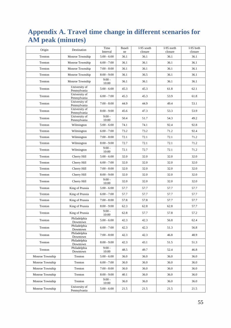
55
Appendix A. Travel time change in different scenarios for
AM peak (minutes)
Origin Destination Time
Interval
Baseli
ne
I-95 south
closure
I-95 north
closure
I-95 both
closure
Trenton Monroe Township 5:00 - 6:00 36.1 36.1 36.1 36.1
Trenton Monroe Township 6:00 - 7:00 36.1 36.1 36.1 36.1
Trenton Monroe Township 7:00 - 8:00 36.1 36.1 36.1 36.1
Trenton Monroe Township 8:00 - 9:00 36.1 36.5 36.1 36.1
Trenton Monroe Township 9:00 -
10:00 36.1 36.1 36.1 36.1
Trenton University of Pennsylvania
5:00 - 6:00 45.3 45.3 61.8 62.1
Trenton University of
Pennsylvania 6:00 - 7:00 45.3 45.3 53.9 61.8
Trenton University of Pennsylvania
7:00 - 8:00 44.9 44.9 49.4 53.1
Trenton University of
Pennsylvania 8:00 - 9:00 45.6 47.3 53.3 53.9
Trenton University of Pennsylvania
9:00 - 10:00
50.4 51.7 54.3 49.2
Trenton Wilmington 5:00 - 6:00 74.1 74.1 92.4 92.8
Trenton Wilmington 6:00 - 7:00 73.2 73.2 71.2 92.4
Trenton Wilmington 7:00 - 8:00 72.1 72.1 72.1 71.2
Trenton Wilmington 8:00 - 9:00 72.7 72.1 72.1 71.2
Trenton Wilmington 9:00 -
10:00 72.1 72.7 72.1 71.2
Trenton Cherry Hill 5:00 - 6:00 32.0 32.0 32.0 32.0
Trenton Cherry Hill 6:00 - 7:00 32.0 32.0 32.0 32.0
Trenton Cherry Hill 7:00 - 8:00 32.0 32.0 32.0 32.0
Trenton Cherry Hill 8:00 - 9:00 32.0 32.0 32.0 32.0
Trenton Cherry Hill 9:00 -
10:00 32.0 32.0 32.0 32.0
Trenton King of Prussia 5:00 - 6:00 57.7 57.7 57.7 57.7
Trenton King of Prussia 6:00 - 7:00 57.7 57.7 57.7 57.7
Trenton King of Prussia 7:00 - 8:00 57.8 57.8 57.7 57.7
Trenton King of Prussia 8:00 - 9:00 62.3 62.8 62.8 57.7
Trenton King of Prussia 9:00 -
10:00 62.8 57.7 57.8 57.2
Trenton Philadelphia Downtown
5:00 - 6:00 42.3 42.3 56.8 62.4
Trenton Philadelphia
Downtown 6:00 - 7:00 42.3 42.3 51.3 56.8
Trenton Philadelphia Downtown
7:00 - 8:00 42.3 42.3 46.8 48.9
Trenton Philadelphia
Downtown 8:00 - 9:00 42.3 43.1 51.5 51.3
Trenton Philadelphia Downtown
9:00 - 10:00
48.5 49.7 52.4 46.8
Monroe Township Trenton 5:00 - 6:00 36.0 36.0 36.0 36.0
Monroe Township Trenton 6:00 - 7:00 36.0 36.0 36.0 36.0
Monroe Township Trenton 7:00 - 8:00 36.0 36.0 36.0 36.0
Monroe Township Trenton 8:00 - 9:00 40.1 36.0 36.0 36.0
Monroe Township Trenton 9:00 - 10:00
36.0 36.0 36.0 36.0
Monroe Township University of
Pennsylvania 5:00 - 6:00 21.5 21.5 21.5 21.5
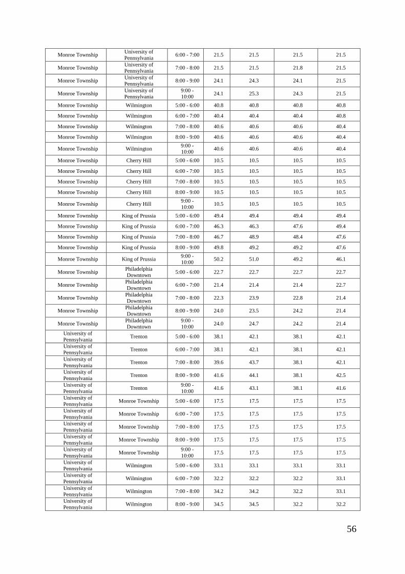
56
Monroe Township University of
Pennsylvania 6:00 - 7:00 21.5 21.5 21.5 21.5
Monroe Township University of Pennsylvania
7:00 - 8:00 21.5 21.5 21.8 21.5
Monroe Township University of
Pennsylvania 8:00 - 9:00 24.1 24.3 24.1 21.5
Monroe Township University of Pennsylvania
9:00 - 10:00
24.1 25.3 24.3 21.5
Monroe Township Wilmington 5:00 - 6:00 40.8 40.8 40.8 40.8
Monroe Township Wilmington 6:00 - 7:00 40.4 40.4 40.4 40.8
Monroe Township Wilmington 7:00 - 8:00 40.6 40.6 40.6 40.4
Monroe Township Wilmington 8:00 - 9:00 40.6 40.6 40.6 40.4
Monroe Township Wilmington 9:00 - 10:00
40.6 40.6 40.6 40.4
Monroe Township Cherry Hill 5:00 - 6:00 10.5 10.5 10.5 10.5
Monroe Township Cherry Hill 6:00 - 7:00 10.5 10.5 10.5 10.5
Monroe Township Cherry Hill 7:00 - 8:00 10.5 10.5 10.5 10.5
Monroe Township Cherry Hill 8:00 - 9:00 10.5 10.5 10.5 10.5
Monroe Township Cherry Hill 9:00 -
10:00 10.5 10.5 10.5 10.5
Monroe Township King of Prussia 5:00 - 6:00 49.4 49.4 49.4 49.4
Monroe Township King of Prussia 6:00 - 7:00 46.3 46.3 47.6 49.4
Monroe Township King of Prussia 7:00 - 8:00 46.7 48.9 48.4 47.6
Monroe Township King of Prussia 8:00 - 9:00 49.8 49.2 49.2 47.6
Monroe Township King of Prussia 9:00 -
10:00 50.2 51.0 49.2 46.1
Monroe Township Philadelphia Downtown
5:00 - 6:00 22.7 22.7 22.7 22.7
Monroe Township Philadelphia
Downtown 6:00 - 7:00 21.4 21.4 21.4 22.7
Monroe Township Philadelphia Downtown
7:00 - 8:00 22.3 23.9 22.8 21.4
Monroe Township Philadelphia
Downtown 8:00 - 9:00 24.0 23.5 24.2 21.4
Monroe Township Philadelphia Downtown
9:00 - 10:00
24.0 24.7 24.2 21.4
University of
Pennsylvania Trenton 5:00 - 6:00 38.1 42.1 38.1 42.1
University of
Pennsylvania Trenton 6:00 - 7:00 38.1 42.1 38.1 42.1
University of
Pennsylvania Trenton 7:00 - 8:00 39.6 43.7 38.1 42.1
University of
Pennsylvania Trenton 8:00 - 9:00 41.6 44.1 38.1 42.5
University of
Pennsylvania Trenton
9:00 -
10:00 41.6 43.1 38.1 41.6
University of
Pennsylvania Monroe Township 5:00 - 6:00 17.5 17.5 17.5 17.5
University of
Pennsylvania Monroe Township 6:00 - 7:00 17.5 17.5 17.5 17.5
University of
Pennsylvania Monroe Township 7:00 - 8:00 17.5 17.5 17.5 17.5
University of
Pennsylvania Monroe Township 8:00 - 9:00 17.5 17.5 17.5 17.5
University of
Pennsylvania Monroe Township
9:00 -
10:00 17.5 17.5 17.5 17.5
University of
Pennsylvania Wilmington 5:00 - 6:00 33.1 33.1 33.1 33.1
University of
Pennsylvania Wilmington 6:00 - 7:00 32.2 32.2 32.2 33.1
University of
Pennsylvania Wilmington 7:00 - 8:00 34.2 34.2 32.2 33.1
University of
Pennsylvania Wilmington 8:00 - 9:00 34.5 34.5 32.2 32.2
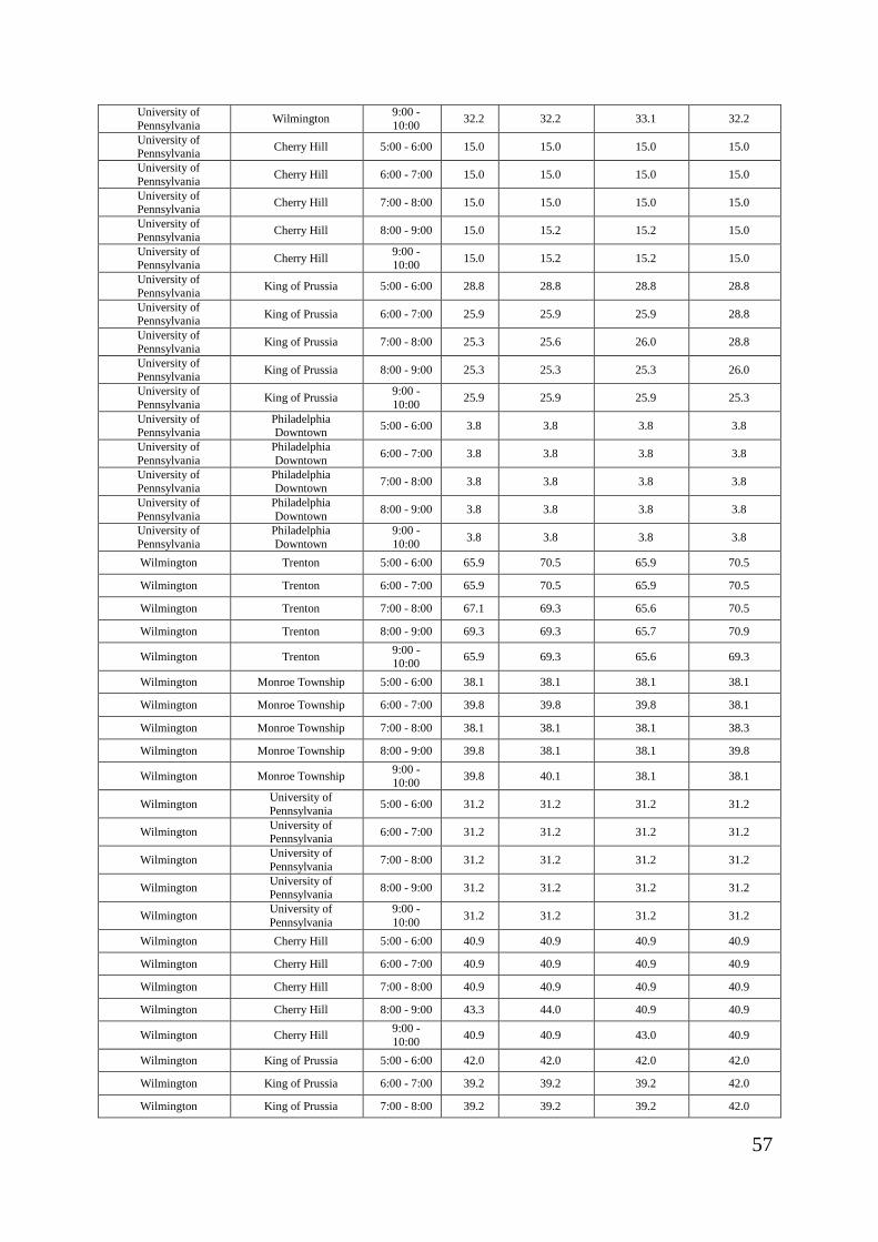
57
University of
Pennsylvania Wilmington
9:00 -
10:00 32.2 32.2 33.1 32.2
University of Pennsylvania
Cherry Hill 5:00 - 6:00 15.0 15.0 15.0 15.0
University of
Pennsylvania Cherry Hill 6:00 - 7:00 15.0 15.0 15.0 15.0
University of Pennsylvania
Cherry Hill 7:00 - 8:00 15.0 15.0 15.0 15.0
University of
Pennsylvania Cherry Hill 8:00 - 9:00 15.0 15.2 15.2 15.0
University of Pennsylvania
Cherry Hill 9:00 - 10:00
15.0 15.2 15.2 15.0
University of
Pennsylvania King of Prussia 5:00 - 6:00 28.8 28.8 28.8 28.8
University of Pennsylvania
King of Prussia 6:00 - 7:00 25.9 25.9 25.9 28.8
University of
Pennsylvania King of Prussia 7:00 - 8:00 25.3 25.6 26.0 28.8
University of Pennsylvania
King of Prussia 8:00 - 9:00 25.3 25.3 25.3 26.0
University of
Pennsylvania King of Prussia
9:00 -
10:00 25.9 25.9 25.9 25.3
University of Pennsylvania
Philadelphia Downtown
5:00 - 6:00 3.8 3.8 3.8 3.8
University of
Pennsylvania
Philadelphia
Downtown 6:00 - 7:00 3.8 3.8 3.8 3.8
University of
Pennsylvania
Philadelphia
Downtown 7:00 - 8:00 3.8 3.8 3.8 3.8
University of
Pennsylvania
Philadelphia
Downtown 8:00 - 9:00 3.8 3.8 3.8 3.8
University of
Pennsylvania
Philadelphia
Downtown
9:00 -
10:00 3.8 3.8 3.8 3.8
Wilmington Trenton 5:00 - 6:00 65.9 70.5 65.9 70.5
Wilmington Trenton 6:00 - 7:00 65.9 70.5 65.9 70.5
Wilmington Trenton 7:00 - 8:00 67.1 69.3 65.6 70.5
Wilmington Trenton 8:00 - 9:00 69.3 69.3 65.7 70.9
Wilmington Trenton 9:00 - 10:00
65.9 69.3 65.6 69.3
Wilmington Monroe Township 5:00 - 6:00 38.1 38.1 38.1 38.1
Wilmington Monroe Township 6:00 - 7:00 39.8 39.8 39.8 38.1
Wilmington Monroe Township 7:00 - 8:00 38.1 38.1 38.1 38.3
Wilmington Monroe Township 8:00 - 9:00 39.8 38.1 38.1 39.8
Wilmington Monroe Township 9:00 - 10:00
39.8 40.1 38.1 38.1
Wilmington University of
Pennsylvania 5:00 - 6:00 31.2 31.2 31.2 31.2
Wilmington University of Pennsylvania
6:00 - 7:00 31.2 31.2 31.2 31.2
Wilmington University of
Pennsylvania 7:00 - 8:00 31.2 31.2 31.2 31.2
Wilmington University of Pennsylvania
8:00 - 9:00 31.2 31.2 31.2 31.2
Wilmington University of
Pennsylvania
9:00 -
10:00 31.2 31.2 31.2 31.2
Wilmington Cherry Hill 5:00 - 6:00 40.9 40.9 40.9 40.9
Wilmington Cherry Hill 6:00 - 7:00 40.9 40.9 40.9 40.9
Wilmington Cherry Hill 7:00 - 8:00 40.9 40.9 40.9 40.9
Wilmington Cherry Hill 8:00 - 9:00 43.3 44.0 40.9 40.9
Wilmington Cherry Hill 9:00 -
10:00 40.9 40.9 43.0 40.9
Wilmington King of Prussia 5:00 - 6:00 42.0 42.0 42.0 42.0
Wilmington King of Prussia 6:00 - 7:00 39.2 39.2 39.2 42.0
Wilmington King of Prussia 7:00 - 8:00 39.2 39.2 39.2 42.0
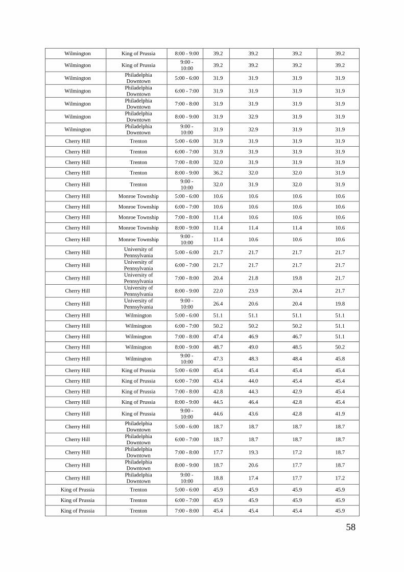
58
Wilmington King of Prussia 8:00 - 9:00 39.2 39.2 39.2 39.2
Wilmington King of Prussia 9:00 -
10:00 39.2 39.2 39.2 39.2
Wilmington Philadelphia Downtown
5:00 - 6:00 31.9 31.9 31.9 31.9
Wilmington Philadelphia
Downtown 6:00 - 7:00 31.9 31.9 31.9 31.9
Wilmington Philadelphia Downtown
7:00 - 8:00 31.9 31.9 31.9 31.9
Wilmington Philadelphia
Downtown 8:00 - 9:00 31.9 32.9 31.9 31.9
Wilmington Philadelphia Downtown
9:00 - 10:00
31.9 32.9 31.9 31.9
Cherry Hill Trenton 5:00 - 6:00 31.9 31.9 31.9 31.9
Cherry Hill Trenton 6:00 - 7:00 31.9 31.9 31.9 31.9
Cherry Hill Trenton 7:00 - 8:00 32.0 31.9 31.9 31.9
Cherry Hill Trenton 8:00 - 9:00 36.2 32.0 32.0 31.9
Cherry Hill Trenton 9:00 -
10:00 32.0 31.9 32.0 31.9
Cherry Hill Monroe Township 5:00 - 6:00 10.6 10.6 10.6 10.6
Cherry Hill Monroe Township 6:00 - 7:00 10.6 10.6 10.6 10.6
Cherry Hill Monroe Township 7:00 - 8:00 11.4 10.6 10.6 10.6
Cherry Hill Monroe Township 8:00 - 9:00 11.4 11.4 11.4 10.6
Cherry Hill Monroe Township 9:00 -
10:00 11.4 10.6 10.6 10.6
Cherry Hill University of Pennsylvania
5:00 - 6:00 21.7 21.7 21.7 21.7
Cherry Hill University of
Pennsylvania 6:00 - 7:00 21.7 21.7 21.7 21.7
Cherry Hill University of Pennsylvania
7:00 - 8:00 20.4 21.8 19.8 21.7
Cherry Hill University of
Pennsylvania 8:00 - 9:00 22.0 23.9 20.4 21.7
Cherry Hill University of Pennsylvania
9:00 - 10:00
26.4 20.6 20.4 19.8
Cherry Hill Wilmington 5:00 - 6:00 51.1 51.1 51.1 51.1
Cherry Hill Wilmington 6:00 - 7:00 50.2 50.2 50.2 51.1
Cherry Hill Wilmington 7:00 - 8:00 47.4 46.9 46.7 51.1
Cherry Hill Wilmington 8:00 - 9:00 48.7 49.0 48.5 50.2
Cherry Hill Wilmington 9:00 - 10:00
47.3 48.3 48.4 45.8
Cherry Hill King of Prussia 5:00 - 6:00 45.4 45.4 45.4 45.4
Cherry Hill King of Prussia 6:00 - 7:00 43.4 44.0 45.4 45.4
Cherry Hill King of Prussia 7:00 - 8:00 42.8 44.3 42.9 45.4
Cherry Hill King of Prussia 8:00 - 9:00 44.5 46.4 42.8 45.4
Cherry Hill King of Prussia 9:00 - 10:00
44.6 43.6 42.8 41.9
Cherry Hill Philadelphia
Downtown 5:00 - 6:00 18.7 18.7 18.7 18.7
Cherry Hill Philadelphia Downtown
6:00 - 7:00 18.7 18.7 18.7 18.7
Cherry Hill Philadelphia
Downtown 7:00 - 8:00 17.7 19.3 17.2 18.7
Cherry Hill Philadelphia Downtown
8:00 - 9:00 18.7 20.6 17.7 18.7
Cherry Hill Philadelphia
Downtown
9:00 -
10:00 18.8 17.4 17.7 17.2
King of Prussia Trenton 5:00 - 6:00 45.9 45.9 45.9 45.9
King of Prussia Trenton 6:00 - 7:00 45.9 45.9 45.9 45.9
King of Prussia Trenton 7:00 - 8:00 45.4 45.4 45.4 45.9
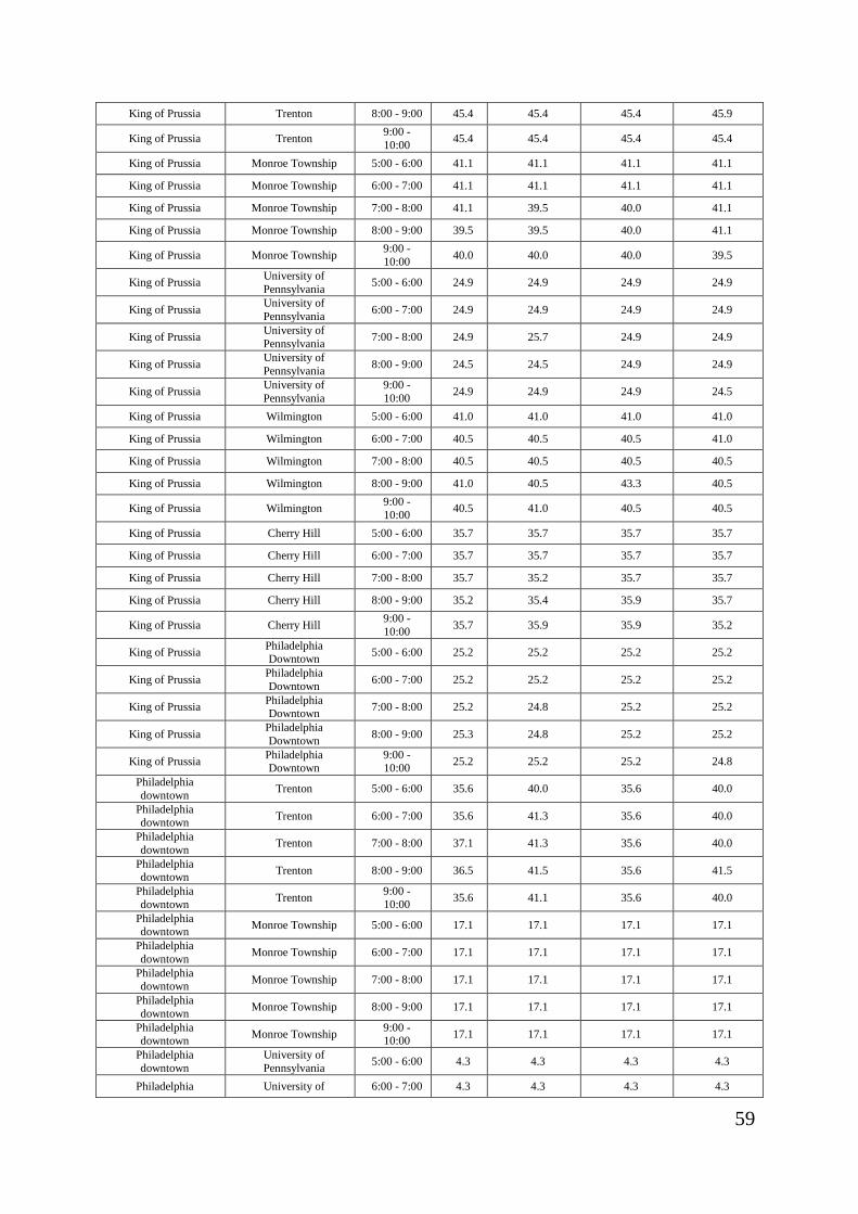
59
King of Prussia Trenton 8:00 - 9:00 45.4 45.4 45.4 45.9
King of Prussia Trenton 9:00 -
10:00 45.4 45.4 45.4 45.4
King of Prussia Monroe Township 5:00 - 6:00 41.1 41.1 41.1 41.1
King of Prussia Monroe Township 6:00 - 7:00 41.1 41.1 41.1 41.1
King of Prussia Monroe Township 7:00 - 8:00 41.1 39.5 40.0 41.1
King of Prussia Monroe Township 8:00 - 9:00 39.5 39.5 40.0 41.1
King of Prussia Monroe Township 9:00 -
10:00 40.0 40.0 40.0 39.5
King of Prussia University of
Pennsylvania 5:00 - 6:00 24.9 24.9 24.9 24.9
King of Prussia University of
Pennsylvania 6:00 - 7:00 24.9 24.9 24.9 24.9
King of Prussia University of
Pennsylvania 7:00 - 8:00 24.9 25.7 24.9 24.9
King of Prussia University of
Pennsylvania 8:00 - 9:00 24.5 24.5 24.9 24.9
King of Prussia University of
Pennsylvania
9:00 -
10:00 24.9 24.9 24.9 24.5
King of Prussia Wilmington 5:00 - 6:00 41.0 41.0 41.0 41.0
King of Prussia Wilmington 6:00 - 7:00 40.5 40.5 40.5 41.0
King of Prussia Wilmington 7:00 - 8:00 40.5 40.5 40.5 40.5
King of Prussia Wilmington 8:00 - 9:00 41.0 40.5 43.3 40.5
King of Prussia Wilmington 9:00 -
10:00 40.5 41.0 40.5 40.5
King of Prussia Cherry Hill 5:00 - 6:00 35.7 35.7 35.7 35.7
King of Prussia Cherry Hill 6:00 - 7:00 35.7 35.7 35.7 35.7
King of Prussia Cherry Hill 7:00 - 8:00 35.7 35.2 35.7 35.7
King of Prussia Cherry Hill 8:00 - 9:00 35.2 35.4 35.9 35.7
King of Prussia Cherry Hill 9:00 -
10:00 35.7 35.9 35.9 35.2
King of Prussia Philadelphia Downtown
5:00 - 6:00 25.2 25.2 25.2 25.2
King of Prussia Philadelphia
Downtown 6:00 - 7:00 25.2 25.2 25.2 25.2
King of Prussia Philadelphia Downtown
7:00 - 8:00 25.2 24.8 25.2 25.2
King of Prussia Philadelphia
Downtown 8:00 - 9:00 25.3 24.8 25.2 25.2
King of Prussia Philadelphia Downtown
9:00 - 10:00
25.2 25.2 25.2 24.8
Philadelphia
downtown Trenton 5:00 - 6:00 35.6 40.0 35.6 40.0
Philadelphia downtown
Trenton 6:00 - 7:00 35.6 41.3 35.6 40.0
Philadelphia
downtown Trenton 7:00 - 8:00 37.1 41.3 35.6 40.0
Philadelphia downtown
Trenton 8:00 - 9:00 36.5 41.5 35.6 41.5
Philadelphia
downtown Trenton
9:00 -
10:00 35.6 41.1 35.6 40.0
Philadelphia downtown
Monroe Township 5:00 - 6:00 17.1 17.1 17.1 17.1
Philadelphia
downtown Monroe Township 6:00 - 7:00 17.1 17.1 17.1 17.1
Philadelphia downtown
Monroe Township 7:00 - 8:00 17.1 17.1 17.1 17.1
Philadelphia
downtown Monroe Township 8:00 - 9:00 17.1 17.1 17.1 17.1
Philadelphia downtown
Monroe Township 9:00 - 10:00
17.1 17.1 17.1 17.1
Philadelphia
downtown
University of
Pennsylvania 5:00 - 6:00 4.3 4.3 4.3 4.3
Philadelphia University of 6:00 - 7:00 4.3 4.3 4.3 4.3
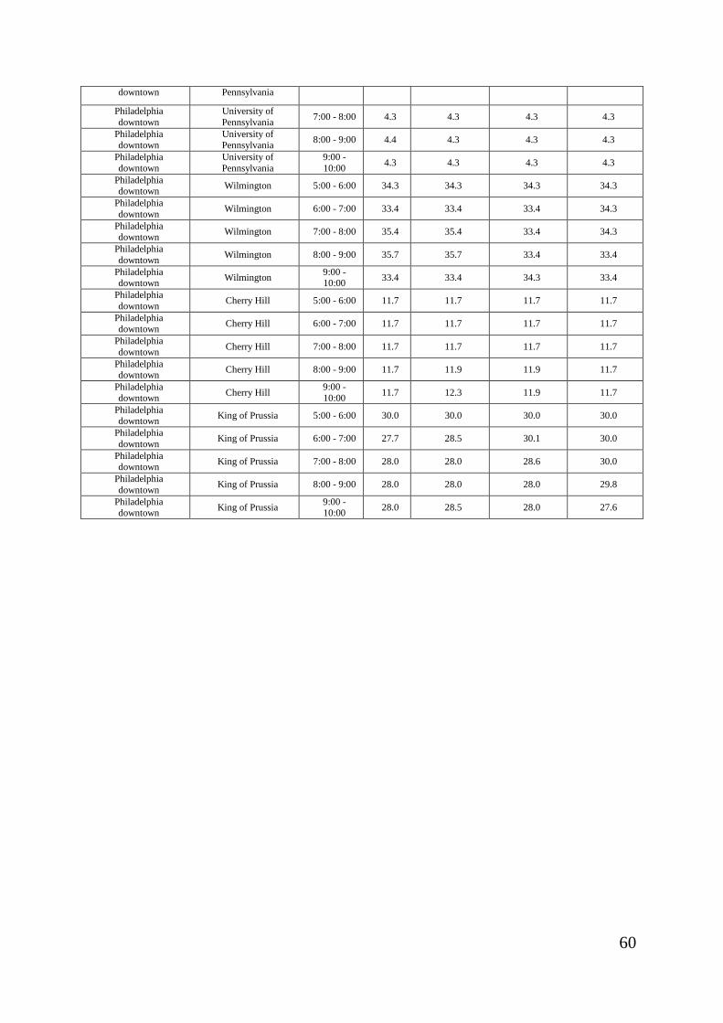
60
downtown Pennsylvania
Philadelphia
downtown
University of
Pennsylvania 7:00 - 8:00 4.3 4.3 4.3 4.3
Philadelphia downtown
University of Pennsylvania
8:00 - 9:00 4.4 4.3 4.3 4.3
Philadelphia
downtown
University of
Pennsylvania
9:00 -
10:00 4.3 4.3 4.3 4.3
Philadelphia downtown
Wilmington 5:00 - 6:00 34.3 34.3 34.3 34.3
Philadelphia
downtown Wilmington 6:00 - 7:00 33.4 33.4 33.4 34.3
Philadelphia downtown
Wilmington 7:00 - 8:00 35.4 35.4 33.4 34.3
Philadelphia
downtown Wilmington 8:00 - 9:00 35.7 35.7 33.4 33.4
Philadelphia downtown
Wilmington 9:00 - 10:00
33.4 33.4 34.3 33.4
Philadelphia
downtown Cherry Hill 5:00 - 6:00 11.7 11.7 11.7 11.7
Philadelphia downtown
Cherry Hill 6:00 - 7:00 11.7 11.7 11.7 11.7
Philadelphia
downtown Cherry Hill 7:00 - 8:00 11.7 11.7 11.7 11.7
Philadelphia downtown
Cherry Hill 8:00 - 9:00 11.7 11.9 11.9 11.7
Philadelphia
downtown Cherry Hill
9:00 -
10:00 11.7 12.3 11.9 11.7
Philadelphia downtown
King of Prussia 5:00 - 6:00 30.0 30.0 30.0 30.0
Philadelphia
downtown King of Prussia 6:00 - 7:00 27.7 28.5 30.1 30.0
Philadelphia downtown
King of Prussia 7:00 - 8:00 28.0 28.0 28.6 30.0
Philadelphia
downtown King of Prussia 8:00 - 9:00 28.0 28.0 28.0 29.8
Philadelphia downtown
King of Prussia 9:00 - 10:00
28.0 28.5 28.0 27.6
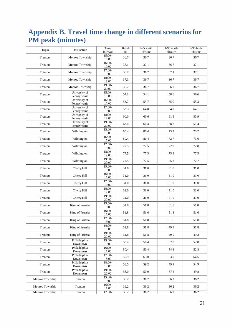
61
Appendix B. Travel time change in different scenarios for
PM peak (minutes)
Origin Destination Time
Interval
Baseli
ne
I-95 south
closure
I-95 north
closure
I-95 both
closure
Trenton Monroe Township 15:00-16:00
36.7 36.7 36.7 36.7
Trenton Monroe Township 16:00-
17:00 37.1 37.1 36.7 37.1
Trenton Monroe Township 17:00-18:00
36.7 36.7 37.1 37.1
Trenton Monroe Township 18:00-
19:00 37.1 36.7 36.7 36.7
Trenton Monroe Township 19:00-20:00
36.7 36.7 36.7 36.7
Trenton University of
Pennsylvania
15:00-
16:00 54.1 54.1 58.6 58.6
Trenton University of Pennsylvania
16:00-17:00
53.7 53.7 65.0 55.3
Trenton University of
Pennsylvania
17:00-
18:00 53.3 64.8 54.9 64.1
Trenton University of Pennsylvania
18:00-19:00
60.0 60.6 51.5 55.9
Trenton University of
Pennsylvania
19:00-
20:00 63.4 60.3 58.8 51.4
Trenton Wilmington 15:00-
16:00 80.4 80.4 73.2 73.2
Trenton Wilmington 16:00-
17:00 80.4 80.4 72.7 73.6
Trenton Wilmington 17:00-
18:00 77.5 77.5 72.8 72.8
Trenton Wilmington 18:00-
19:00 77.5 77.5 75.2 77.5
Trenton Wilmington 19:00-
20:00 77.5 77.5 75.2 72.7
Trenton Cherry Hill 15:00-
16:00 31.0 31.0 31.0 31.0
Trenton Cherry Hill 16:00-
17:00 31.0 31.0 31.0 31.0
Trenton Cherry Hill 17:00-
18:00 31.0 31.0 31.0 31.0
Trenton Cherry Hill 18:00-
19:00 31.0 31.0 31.0 31.0
Trenton Cherry Hill 19:00-
20:00 31.0 31.0 31.0 31.0
Trenton King of Prussia 15:00-
16:00 51.8 51.8 51.8 51.8
Trenton King of Prussia 16:00-
17:00 51.8 51.6 51.8 51.6
Trenton King of Prussia 17:00-
18:00 51.8 51.8 51.6 51.8
Trenton King of Prussia 18:00-19:00
51.8 51.8 49.5 51.8
Trenton King of Prussia 19:00-
20:00 51.8 51.8 49.5 49.3
Trenton Philadelphia Downtown
15:00-16:00
50.4 50.4 52.8 52.8
Trenton Philadelphia
Downtown
16:00-
17:00 50.4 50.4 54.6 52.8
Trenton Philadelphia
Downtown
17:00-
18:00 50.9 63.0 53.0 64.5
Trenton Philadelphia
Downtown
18:00-
19:00 58.5 59.2 49.9 54.9
Trenton Philadelphia Downtown
19:00-20:00
58.0 50.9 57.2 49.8
Monroe Township Trenton 15:00-
16:00 36.2 36.2 36.2 36.2
Monroe Township Trenton 16:00-17:00
36.2 36.2 36.2 36.2
Monroe Township Trenton 17:00- 36.2 36.2 36.2 36.2
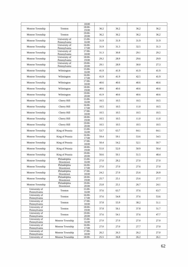
62
18:00
Monroe Township Trenton 18:00-
19:00 36.2 36.2 36.2 36.2
Monroe Township Trenton 19:00-
20:00 36.2 36.2 36.2 36.2
Monroe Township University of
Pennsylvania
15:00-
16:00 31.9 31.9 31.9 31.9
Monroe Township University of
Pennsylvania
16:00-
17:00 31.9 31.3 32.5 31.3
Monroe Township University of
Pennsylvania
17:00-
18:00 31.3 30.8 29.1 29.2
Monroe Township University of
Pennsylvania
18:00-
19:00 29.2 28.9 29.6 29.9
Monroe Township University of
Pennsylvania
19:00-
20:00 29.1 28.9 30.0 27.3
Monroe Township Wilmington 15:00-
16:00 41.9 41.9 41.9 41.9
Monroe Township Wilmington 16:00-
17:00 41.9 41.9 42.5 41.9
Monroe Township Wilmington 17:00-
18:00 40.6 40.6 40.6 40.6
Monroe Township Wilmington 18:00-
19:00 40.6 40.6 40.6 40.6
Monroe Township Wilmington 19:00-
20:00 41.9 40.6 40.6 40.6
Monroe Township Cherry Hill 15:00-16:00
10.5 10.5 10.5 10.5
Monroe Township Cherry Hill 16:00-
17:00 10.5 10.5 11.0 10.5
Monroe Township Cherry Hill 17:00-18:00
10.5 10.5 10.5 10.5
Monroe Township Cherry Hill 18:00-
19:00 10.5 10.5 11.0 11.0
Monroe Township Cherry Hill 19:00-20:00
10.5 10.5 10.5 10.5
Monroe Township King of Prussia 15:00-
16:00 53.7 63.7 64.1 64.1
Monroe Township King of Prussia 16:00-17:00
59.4 59.1 53.6 54.5
Monroe Township King of Prussia 17:00-
18:00 50.4 54.2 52.1 50.7
Monroe Township King of Prussia 18:00-
19:00 51.0 52.0 50.9 50.4
Monroe Township King of Prussia 19:00-
20:00 50.6 50.1 51.5 48.4
Monroe Township Philadelphia Downtown
15:00-16:00
27.0 28.2 27.0 27.0
Monroe Township Philadelphia
Downtown
16:00-
17:00 27.0 27.0 27.6 27.0
Monroe Township Philadelphia Downtown
17:00-18:00
24.2 27.0 25.6 26.8
Monroe Township Philadelphia
Downtown
18:00-
19:00 25.7 25.1 25.6 27.7
Monroe Township Philadelphia Downtown
19:00-20:00
25.8 25.1 26.7 24.1
University of
Pennsylvania Trenton
15:00-
16:00 37.6 63.7 37.6 63.7
University of Pennsylvania
Trenton 16:00-17:00
37.6 54.8 37.6 53.6
University of
Pennsylvania Trenton
17:00-
18:00 37.8 55.9 38.2 51.1
University of
Pennsylvania Trenton
18:00-
19:00 37.8 56.1 37.8 51.7
University of
Pennsylvania Trenton
19:00-
20:00 37.6 54.1 37.6 47.7
University of Pennsylvania
Monroe Township 15:00-16:00
27.0 27.0 27.0 27.0
University of
Pennsylvania Monroe Township
16:00-
17:00 27.0 27.0 27.7 27.0
University of Pennsylvania
Monroe Township 17:00-18:00
26.2 26.3 26.2 27.0
University of Monroe Township 18:00- 25.5 26.8 26.2 26.1
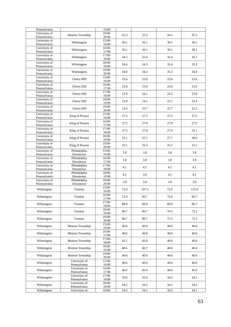
63
Pennsylvania 19:00
University of
Pennsylvania Monroe Township
19:00-
20:00 25.3 25.3 26.1 25.3
University of
Pennsylvania Wilmington
15:00-
16:00 36.1 36.1 36.1 36.1
University of
Pennsylvania Wilmington
16:00-
17:00 36.1 36.1 36.1 36.1
University of
Pennsylvania Wilmington
17:00-
18:00 34.3 35.4 35.4 36.1
University of
Pennsylvania Wilmington
18:00-
19:00 34.4 34.3 35.4 35.3
University of
Pennsylvania Wilmington
19:00-
20:00 34.0 34.2 35.3 34.0
University of
Pennsylvania Cherry Hill
15:00-
16:00 23.6 23.6 23.6 23.6
University of
Pennsylvania Cherry Hill
16:00-
17:00 23.6 23.6 23.6 23.6
University of
Pennsylvania Cherry Hill
17:00-
18:00 23.8 24.1 24.2 23.8
University of
Pennsylvania Cherry Hill
18:00-
19:00 23.8 24.1 23.1 23.4
University of
Pennsylvania Cherry Hill
19:00-
20:00 23.6 23.7 22.7 22.2
University of
Pennsylvania King of Prussia
15:00-
16:00 27.5 27.5 27.5 27.5
University of Pennsylvania
King of Prussia 16:00-17:00
27.5 27.8 27.8 27.5
University of
Pennsylvania King of Prussia
17:00-
18:00 27.5 27.8 27.9 25.1
University of Pennsylvania
King of Prussia 18:00-19:00
25.1 25.1 27.7 28.0
University of
Pennsylvania King of Prussia
19:00-
20:00 25.1 25.3 25.1 25.1
University of Pennsylvania
Philadelphia Downtown
15:00-16:00
3.8 3.8 3.8 3.8
University of
Pennsylvania
Philadelphia
Downtown
16:00-
17:00 3.8 3.8 3.8 3.8
University of Pennsylvania
Philadelphia Downtown
17:00-18:00
4.1 4.1 4.1 4.1
University of
Pennsylvania
Philadelphia
Downtown
18:00-
19:00 4.1 3.8 4.1 4.1
University of
Pennsylvania
Philadelphia
Downtown
19:00-
20:00 3.8 3.8 3.8 3.8
Wilmington Trenton 15:00-
16:00 72.0 107.3 72.0 115.9
Wilmington Trenton 16:00-17:00
72.0 86.7 72.0 86.7
Wilmington Trenton 17:00-
18:00 89.9 89.9 89.9 86.7
Wilmington Trenton 18:00-19:00
86.7 86.7 70.3 72.2
Wilmington Trenton 19:00-
20:00 86.7 86.7 72.2 72.2
Wilmington Monroe Township 15:00-16:00
40.6 40.6 40.6 40.6
Wilmington Monroe Township 16:00-
17:00 40.6 40.8 40.6 40.6
Wilmington Monroe Township 17:00-18:00
42.1 42.0 40.6 40.6
Wilmington Monroe Township 18:00-
19:00 40.6 40.7 40.6 40.6
Wilmington Monroe Township 19:00-
20:00 40.6 40.6 40.6 40.6
Wilmington University of
Pennsylvania
15:00-
16:00 46.6 46.6 46.6 46.6
Wilmington University of Pennsylvania
16:00-17:00
46.6 45.9 46.6 45.9
Wilmington University of
Pennsylvania
17:00-
18:00 35.6 35.6 34.2 34.2
Wilmington University of Pennsylvania
18:00-19:00
34.2 34.2 34.1 34.2
Wilmington University of 19:00- 34.2 34.2 34.2 34.1
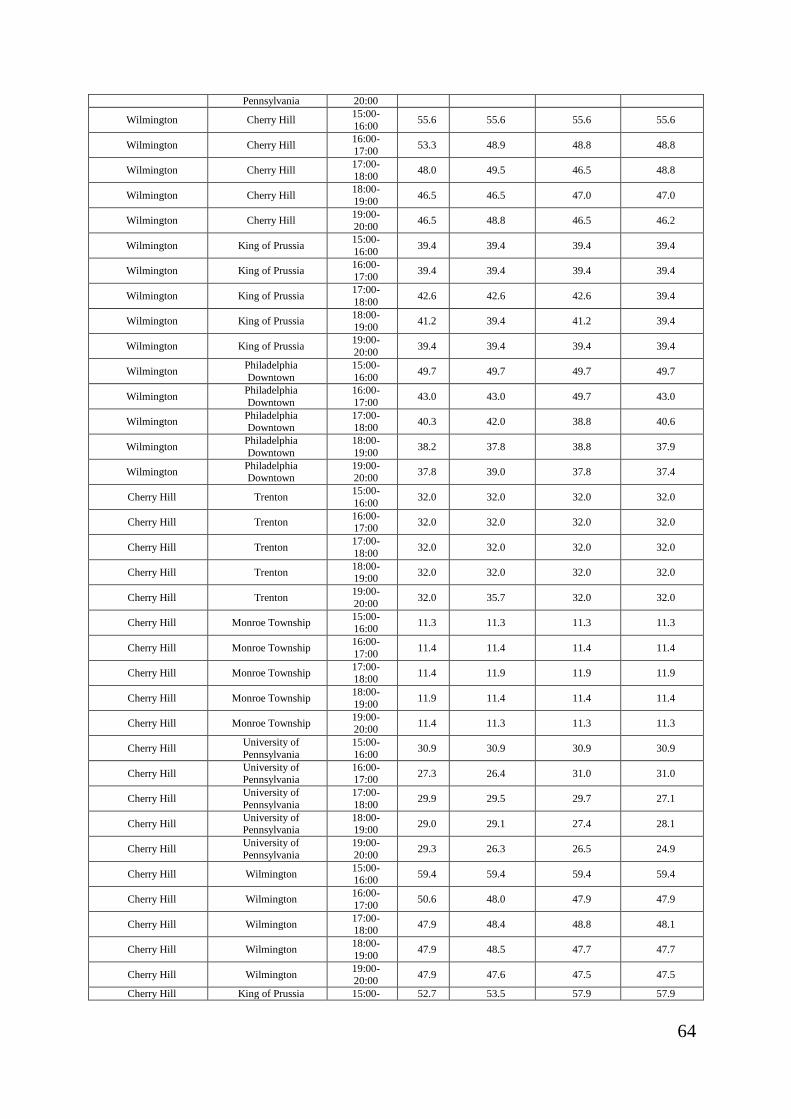
64
Pennsylvania 20:00
Wilmington Cherry Hill 15:00-
16:00 55.6 55.6 55.6 55.6
Wilmington Cherry Hill 16:00-
17:00 53.3 48.9 48.8 48.8
Wilmington Cherry Hill 17:00-
18:00 48.0 49.5 46.5 48.8
Wilmington Cherry Hill 18:00-
19:00 46.5 46.5 47.0 47.0
Wilmington Cherry Hill 19:00-
20:00 46.5 48.8 46.5 46.2
Wilmington King of Prussia 15:00-
16:00 39.4 39.4 39.4 39.4
Wilmington King of Prussia 16:00-
17:00 39.4 39.4 39.4 39.4
Wilmington King of Prussia 17:00-
18:00 42.6 42.6 42.6 39.4
Wilmington King of Prussia 18:00-
19:00 41.2 39.4 41.2 39.4
Wilmington King of Prussia 19:00-
20:00 39.4 39.4 39.4 39.4
Wilmington Philadelphia
Downtown
15:00-
16:00 49.7 49.7 49.7 49.7
Wilmington Philadelphia
Downtown
16:00-
17:00 43.0 43.0 49.7 43.0
Wilmington Philadelphia Downtown
17:00-18:00
40.3 42.0 38.8 40.6
Wilmington Philadelphia
Downtown
18:00-
19:00 38.2 37.8 38.8 37.9
Wilmington Philadelphia Downtown
19:00-20:00
37.8 39.0 37.8 37.4
Cherry Hill Trenton 15:00-
16:00 32.0 32.0 32.0 32.0
Cherry Hill Trenton 16:00-17:00
32.0 32.0 32.0 32.0
Cherry Hill Trenton 17:00-
18:00 32.0 32.0 32.0 32.0
Cherry Hill Trenton 18:00-19:00
32.0 32.0 32.0 32.0
Cherry Hill Trenton 19:00-
20:00 32.0 35.7 32.0 32.0
Cherry Hill Monroe Township 15:00-
16:00 11.3 11.3 11.3 11.3
Cherry Hill Monroe Township 16:00-
17:00 11.4 11.4 11.4 11.4
Cherry Hill Monroe Township 17:00-18:00
11.4 11.9 11.9 11.9
Cherry Hill Monroe Township 18:00-
19:00 11.9 11.4 11.4 11.4
Cherry Hill Monroe Township 19:00-20:00
11.4 11.3 11.3 11.3
Cherry Hill University of
Pennsylvania
15:00-
16:00 30.9 30.9 30.9 30.9
Cherry Hill University of Pennsylvania
16:00-17:00
27.3 26.4 31.0 31.0
Cherry Hill University of
Pennsylvania
17:00-
18:00 29.9 29.5 29.7 27.1
Cherry Hill University of Pennsylvania
18:00-19:00
29.0 29.1 27.4 28.1
Cherry Hill University of
Pennsylvania
19:00-
20:00 29.3 26.3 26.5 24.9
Cherry Hill Wilmington 15:00-
16:00 59.4 59.4 59.4 59.4
Cherry Hill Wilmington 16:00-
17:00 50.6 48.0 47.9 47.9
Cherry Hill Wilmington 17:00-18:00
47.9 48.4 48.8 48.1
Cherry Hill Wilmington 18:00-
19:00 47.9 48.5 47.7 47.7
Cherry Hill Wilmington 19:00-20:00
47.9 47.6 47.5 47.5
Cherry Hill King of Prussia 15:00- 52.7 53.5 57.9 57.9
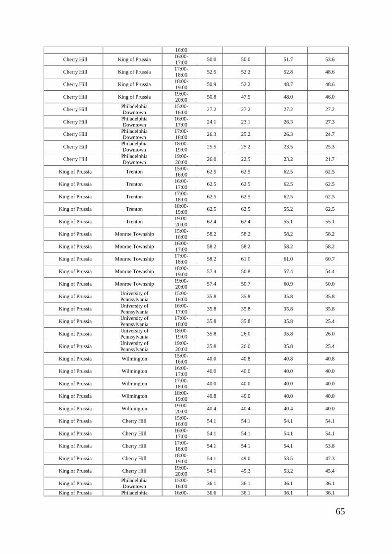
65
16:00
Cherry Hill King of Prussia 16:00-
17:00 50.0 50.0 51.7 53.6
Cherry Hill King of Prussia 17:00-
18:00 52.5 52.2 52.8 48.6
Cherry Hill King of Prussia 18:00-
19:00 50.9 52.2 48.7 48.6
Cherry Hill King of Prussia 19:00-
20:00 50.8 47.5 48.0 46.0
Cherry Hill Philadelphia
Downtown
15:00-
16:00 27.2 27.2 27.2 27.2
Cherry Hill Philadelphia
Downtown
16:00-
17:00 24.1 23.1 26.3 27.3
Cherry Hill Philadelphia
Downtown
17:00-
18:00 26.3 25.2 26.3 24.7
Cherry Hill Philadelphia
Downtown
18:00-
19:00 25.5 25.2 23.5 25.3
Cherry Hill Philadelphia
Downtown
19:00-
20:00 26.0 22.5 23.2 21.7
King of Prussia Trenton 15:00-
16:00 62.5 62.5 62.5 62.5
King of Prussia Trenton 16:00-
17:00 62.5 62.5 62.5 62.5
King of Prussia Trenton 17:00-
18:00 62.5 62.5 62.5 62.5
King of Prussia Trenton 18:00-19:00
62.5 62.5 55.2 62.5
King of Prussia Trenton 19:00-
20:00 62.4 62.4 55.1 55.1
King of Prussia Monroe Township 15:00-16:00
58.2 58.2 58.2 58.2
King of Prussia Monroe Township 16:00-
17:00 58.2 58.2 58.2 58.2
King of Prussia Monroe Township 17:00-18:00
58.2 61.0 61.0 60.7
King of Prussia Monroe Township 18:00-
19:00 57.4 50.8 57.4 54.4
King of Prussia Monroe Township 19:00-20:00
57.4 50.7 60.9 50.0
King of Prussia University of
Pennsylvania
15:00-
16:00 35.8 35.8 35.8 35.8
King of Prussia University of
Pennsylvania
16:00-
17:00 35.8 35.8 35.8 35.8
King of Prussia University of
Pennsylvania
17:00-
18:00 35.8 35.8 35.8 25.4
King of Prussia University of Pennsylvania
18:00-19:00
35.8 26.0 35.8 26.0
King of Prussia University of
Pennsylvania
19:00-
20:00 35.8 26.0 35.8 25.4
King of Prussia Wilmington 15:00-16:00
40.0 40.8 40.8 40.8
King of Prussia Wilmington 16:00-
17:00 40.0 40.0 40.0 40.0
King of Prussia Wilmington 17:00-18:00
40.0 40.0 40.0 40.0
King of Prussia Wilmington 18:00-
19:00 40.8 40.0 40.0 40.0
King of Prussia Wilmington 19:00-20:00
40.4 40.4 40.4 40.0
King of Prussia Cherry Hill 15:00-
16:00 54.1 54.1 54.1 54.1
King of Prussia Cherry Hill 16:00-
17:00 54.1 54.1 54.1 54.1
King of Prussia Cherry Hill 17:00-
18:00 54.1 54.1 54.1 53.8
King of Prussia Cherry Hill 18:00-19:00
54.1 49.0 53.5 47.3
King of Prussia Cherry Hill 19:00-
20:00 54.1 49.3 53.2 45.4
King of Prussia Philadelphia Downtown
15:00-16:00
36.1 36.1 36.1 36.1
King of Prussia Philadelphia 16:00- 36.6 36.1 36.1 36.1
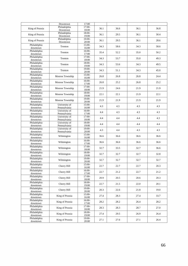
66
Downtown 17:00
King of Prussia Philadelphia
Downtown
17:00-
18:00 36.1 36.6 36.1 36.8
King of Prussia Philadelphia
Downtown
18:00-
19:00 36.1 29.5 36.1 30.4
King of Prussia Philadelphia
Downtown
19:00-
20:00 36.1 29.5 36.1 28.6
Philadelphia
downtown Trenton
15:00-
16:00 34.3 58.6 34.3 58.6
Philadelphia
downtown Trenton
16:00-
17:00 35.4 52.2 35.0 50.2
Philadelphia
downtown Trenton
17:00-
18:00 34.3 53.7 35.0 49.3
Philadelphia
downtown Trenton
18:00-
19:00 34.3 53.6 34.3 49.5
Philadelphia
downtown Trenton
19:00-
20:00 34.3 51.1 34.3 45.0
Philadelphia
downtown Monroe Township
15:00-
16:00 26.8 26.8 26.8 24.4
Philadelphia
downtown Monroe Township
16:00-
17:00 26.8 25.2 26.8 25.2
Philadelphia
downtown Monroe Township
17:00-
18:00 21.9 24.6 21.9 21.9
Philadelphia
downtown Monroe Township
18:00-
19:00 22.1 22.1 21.9 22.1
Philadelphia downtown
Monroe Township 19:00-20:00
21.9 21.9 21.9 21.9
Philadelphia
downtown
University of
Pennsylvania
15:00-
16:00 4.3 4.3 4.3 4.3
Philadelphia downtown
University of Pennsylvania
16:00-17:00
4.4 4.3 4.3 4.3
Philadelphia
downtown
University of
Pennsylvania
17:00-
18:00 4.4 4.4 4.4 4.3
Philadelphia downtown
University of Pennsylvania
18:00-19:00
4.4 4.4 4.4 4.4
Philadelphia
downtown
University of
Pennsylvania
19:00-
20:00 4.3 4.4 4.3 4.3
Philadelphia downtown
Wilmington 15:00-16:00
36.6 36.6 36.6 36.6
Philadelphia
downtown Wilmington
16:00-
17:00 36.6 36.6 36.6 36.6
Philadelphia
downtown Wilmington
17:00-
18:00 32.7 33.5 32.7 36.6
Philadelphia
downtown Wilmington
18:00-
19:00 32.7 32.7 32.7 32.8
Philadelphia downtown
Wilmington 19:00-20:00
32.7 32.7 32.7 32.7
Philadelphia
downtown Cherry Hill
15:00-
16:00 22.7 22.7 22.7 20.3
Philadelphia downtown
Cherry Hill 16:00-17:00
22.7 21.2 22.7 21.2
Philadelphia
downtown Cherry Hill
17:00-
18:00 20.9 20.5 20.6 20.3
Philadelphia downtown
Cherry Hill 18:00-19:00
22.7 21.5 22.0 20.1
Philadelphia
downtown Cherry Hill
19:00-
20:00 20.3 22.6 21.8 19.0
Philadelphia downtown
King of Prussia 15:00-16:00
27.4 28.3 27.4 33.7
Philadelphia
downtown King of Prussia
16:00-
17:00 28.2 28.2 26.4 28.2
Philadelphia
downtown King of Prussia
17:00-
18:00 28.3 28.3 28.7 27.0
Philadelphia
downtown King of Prussia
18:00-
19:00 27.4 29.5 26.9 26.4
Philadelphia downtown
King of Prussia 19:00-20:00
27.1 27.6 27.1 26.4
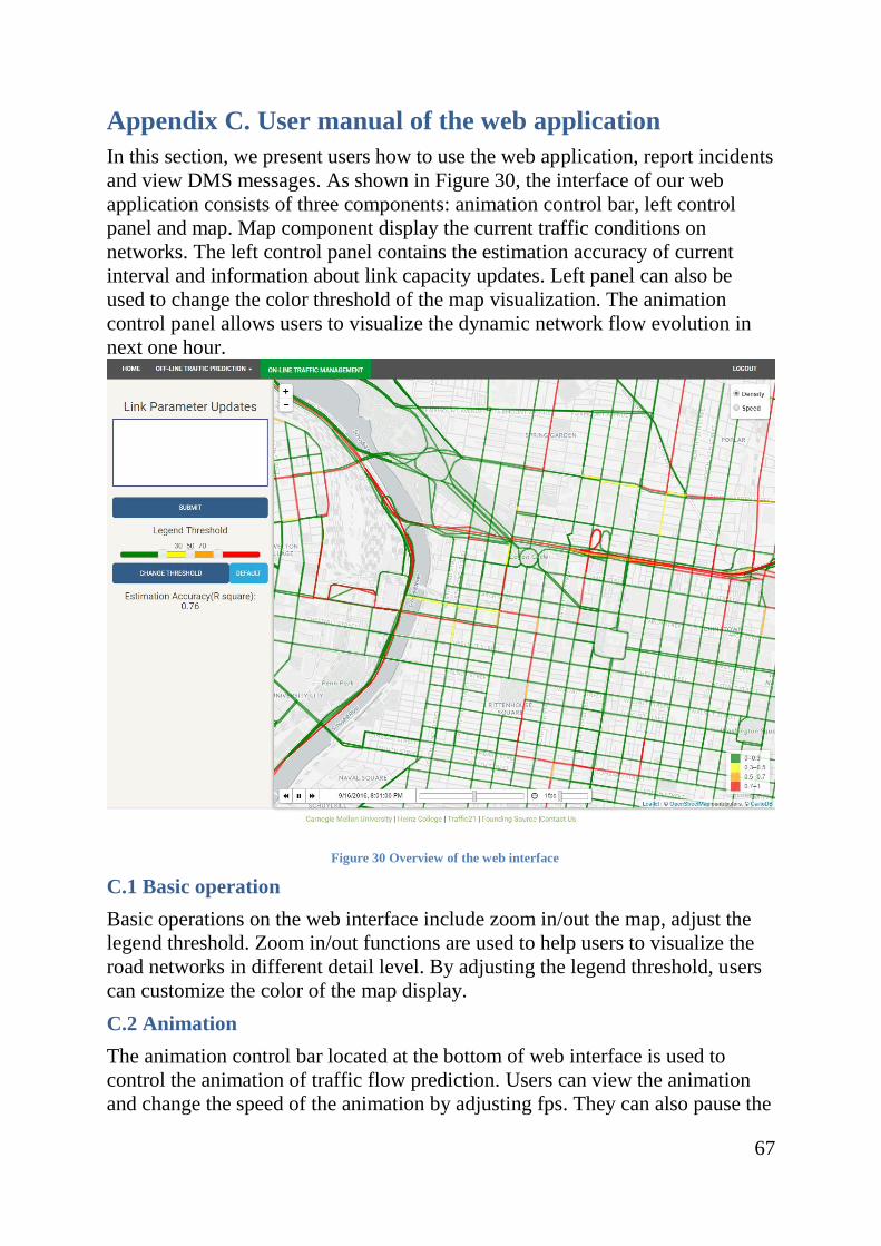
67
Appendix C. User manual of the web application
In this section, we present users how to use the web application, report incidents
and view DMS messages. As shown in Figure 30, the interface of our web
application consists of three components: animation control bar, left control
panel and map. Map component display the current traffic conditions on
networks. The left control panel contains the estimation accuracy of current
interval and information about link capacity updates. Left panel can also be
used to change the color threshold of the map visualization. The animation
control panel allows users to visualize the dynamic network flow evolution in
next one hour.
Figure 30 Overview of the web interface
C.1 Basic operation
Basic operations on the web interface include zoom in/out the map, adjust the
legend threshold. Zoom in/out functions are used to help users to visualize the
road networks in different detail level. By adjusting the legend threshold, users
can customize the color of the map display.
C.2 Animation
The animation control bar located at the bottom of web interface is used to
control the animation of traffic flow prediction. Users can view the animation
and change the speed of the animation by adjusting fps. They can also pause the
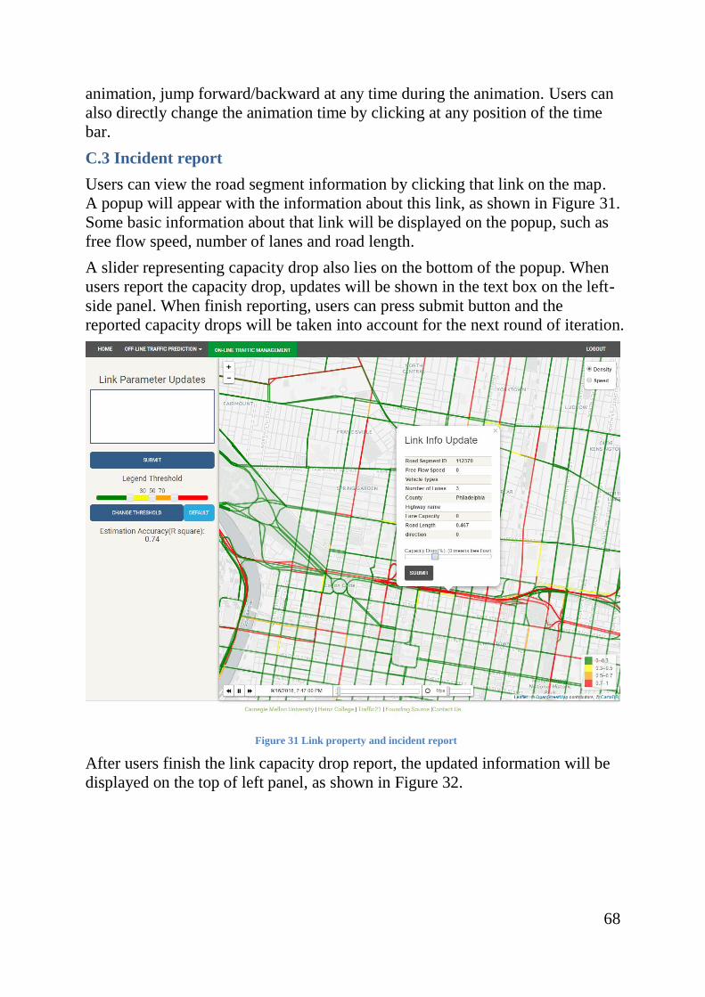
68
animation, jump forward/backward at any time during the animation. Users can
also directly change the animation time by clicking at any position of the time
bar.
C.3 Incident report
Users can view the road segment information by clicking that link on the map.
A popup will appear with the information about this link, as shown in Figure 31.
Some basic information about that link will be displayed on the popup, such as
free flow speed, number of lanes and road length.
A slider representing capacity drop also lies on the bottom of the popup. When
users report the capacity drop, updates will be shown in the text box on the left-
side panel. When finish reporting, users can press submit button and the
reported capacity drops will be taken into account for the next round of iteration.
Figure 31 Link property and incident report
After users finish the link capacity drop report, the updated information will be
displayed on the top of left panel, as shown in Figure 32.
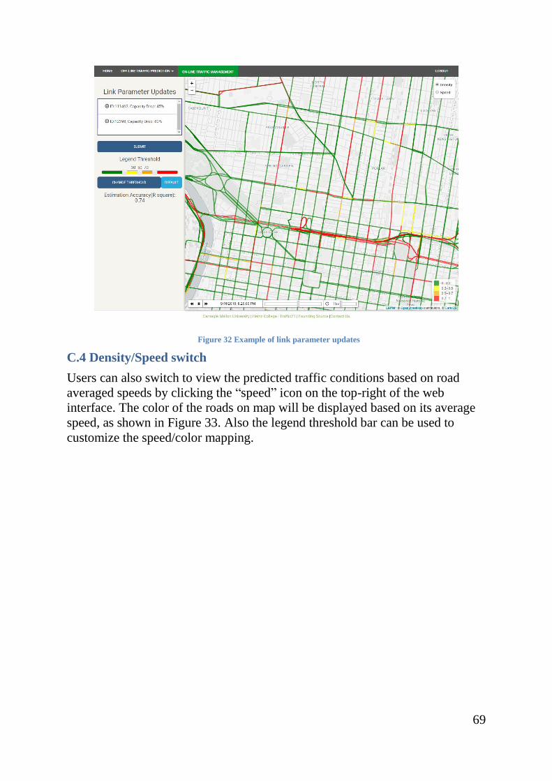
69
Figure 32 Example of link parameter updates
C.4 Density/Speed switch
Users can also switch to view the predicted traffic conditions based on road
averaged speeds by clicking the “speed” icon on the top-right of the web
interface. The color of the roads on map will be displayed based on its average
speed, as shown in Figure 33. Also the legend threshold bar can be used to
customize the speed/color mapping.
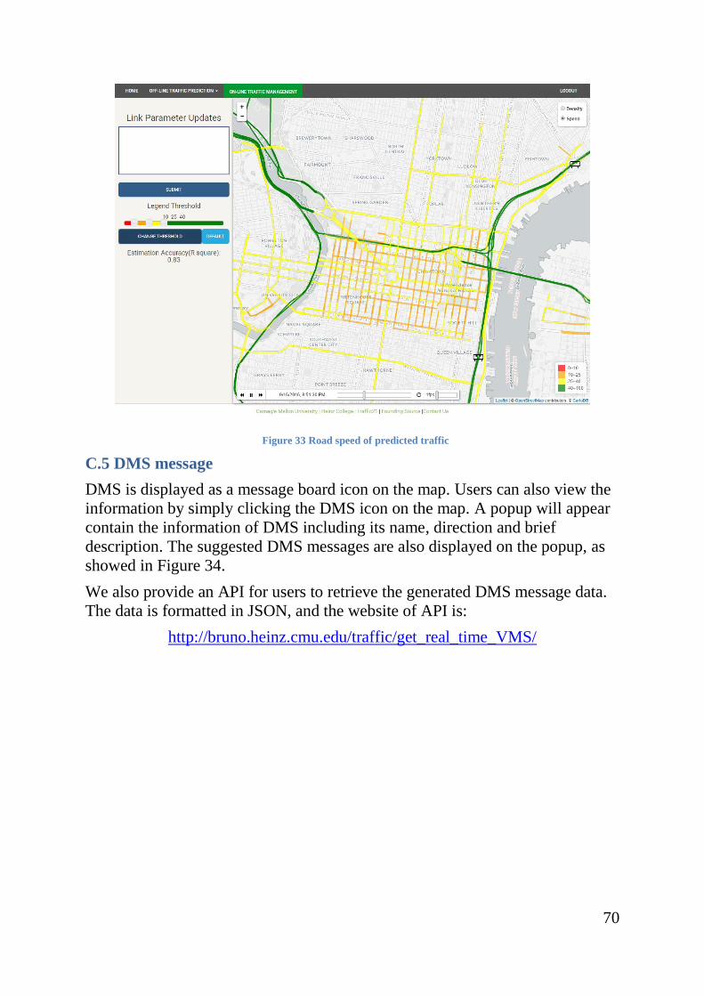
70
Figure 33 Road speed of predicted traffic
C.5 DMS message
DMS is displayed as a message board icon on the map. Users can also view the
information by simply clicking the DMS icon on the map. A popup will appear
contain the information of DMS including its name, direction and brief
description. The suggested DMS messages are also displayed on the popup, as
showed in Figure 34.
We also provide an API for users to retrieve the generated DMS message data.
The data is formatted in JSON, and the website of API is:
http://bruno.heinz.cmu.edu/traffic/get_real_time_VMS/
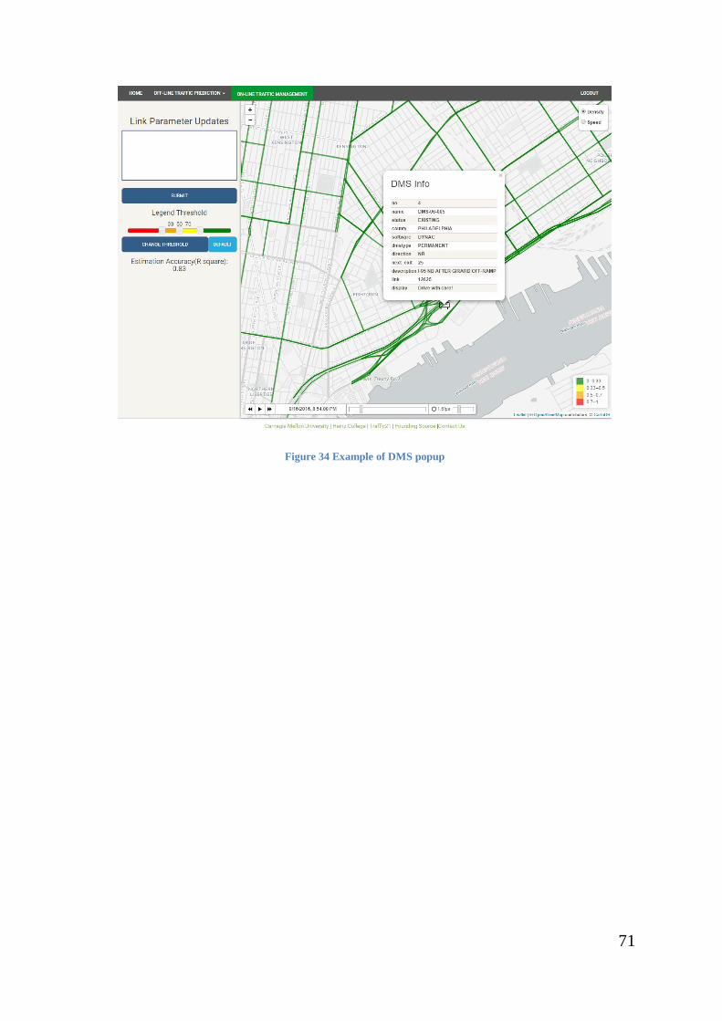
71
Figure 34 Example of DMS popup
Recommended