Computers and Structures 82 (2004) 1719–1736
www.elsevier.com/locate/compstruc
Dynamic FE analysis of South Memnon Colossusincluding 3D soil–foundation–structure interaction
Sara Casciati *, Ronaldo I. Borja
Department of Civil and Environmental Engineering, Stanford University, Stanford, CA 94305-4020, USA
Received 9 July 2003; accepted 10 February 2004
Available online 15 June 2004
Abstract
A full three-dimensional dynamic soil–foundation–structure interaction (SFSI) analysis of a famous landmark in
Luxor, Egypt, the South Memnon Colossus, is performed to investigate the response of this historical monument to
seismic excitation. The analysis is carried out using the finite element (FE) method in time domain. The statue com-
prising the upper structure is modeled using 3D brick finite elements constructed from a photogrammetric represen-
tation that captures important details of the surface and allows the identification of probable zones of stress
concentration. The modeling also takes into account the presence of a surface of discontinuity between the upper part
of the statue and its fractured base. FE models of the foundation and the surrounding soil deposit are constructed and
coupled with the statue model to analyze the seismic response of the entire system incorporating dynamic SFSI effects.
These studies are useful for future conservation efforts of this historical landmark, and more specifically for designing
possible retrofit measures for the fractured base to prevent potential collapse of the monument from overturning during
an earthquake.
� 2004 Elsevier Ltd. All rights reserved.
Keywords: Soil–foundation–structure interaction; Multi-body deformable contact; Non-linear dynamic finite element analysis
1. Introduction
The Memnon Colossi are two huge statues (18 m)
built in Thebes by the pharaoh Amenothep III (18th
Dynasty) to guard the entrance of an ancient mortuary
temple on the eastern side of the river Nile, now known
as the city of Luxor (Fig. 1). The statues resemble the
pharaoh sitting on his throne in regal position with his
hands on his knees; his wife, Tiyi, and his mother,
Moutemouisa, stand at the sides of the throne in smaller
scales. They were called the Colossi of Memnon in
Greek times, when they decided that the statues repre-
* Corresponding author. Address: Department of Structural
Mechanics, University of Pavia, Via Ferrata 1, Pavia 27100,
Italy. Tel.: +39-0382-505458; fax: +39-0382-528422.
E-mail address: [email protected] (S. Casciati).
0045-7949/$ - see front matter � 2004 Elsevier Ltd. All rights reserv
doi:10.1016/j.compstruc.2004.02.026
sented their hero, Memnon. He was a king of Ethiopia
and son of the the dawn god Eos, who died in the hands
of Achilles. After an earthquake in 27 B.C., one of the
statues on the northern side produced a musical sound
under certain weather conditions. Egyptians thought
this sound came from the gods, and Greeks thought it
was Memnon’s voice. Unfortunately, two centuries later
(199 A.D.) the Roman emperor Settimio Severo repaired
the damaged statue, and since then the sound has never
been heard again. The earthquake and several floods
have since wiped out most of the other ruins of the
temple, and now only these monuments and the soil
remain.
The interest in the south statue arises from its origi-
nal and unaltered but severely damaged state. In par-
ticular, the blocks comprising the base of the statue are
severely fractured and must be fastened together or the
entire structure could topple during an earthquake.
ed.

Fig. 2. Model by Verdel and co-workers showing the monu-
ment represented by three parallelepipeds.
Fig. 1. South (left) and North (right) Memnon Colossi in
Luxor, Egypt.
1720 S. Casciati, R.I. Borja / Computers and Structures 82 (2004) 1719–1736
Remedial measures have been proposed to fix the
problem, including stitching the blocks together by
shape memory alloy devices in the form of wires.
However, planning a good retrofit operation requires
careful and accurate modeling of the seismic response of
the structure. We believe that with the advances in
computational methods it is now possible to predict with
reasonable accuracy the seismic demands on this geo-
metrically complex monument. Specifically, computer
modeling and simulations are very useful tools for
identifying regions of stress concentration where only
non-invasive techniques are allowed. Accurate quantifi-
cation of stresses are also useful for understanding the
direction of crack propagation and for quantifying the
seismic demands on whatever new materials may be
introduced in the retrofit program.
The only computational modeling known to the au-
thors of the seismic response of the South Memnon
Colossus was the FE analysis by Verdel and co-workers
[1–3]. The statue was represented by three parallelepi-
peds, one representing the base and two representing
the upper structure, resulting in an overestimation of
the volume of the statue by about 30% (Fig. 2). The
underlying foundation was represented by elastic layers
of silt and limestone 6 and 24.5 m in thickness, respec-
tively. The analysis utilized a vertical plane of symmetry
between the two statues so that only one statue had to be
analyzed. Strictly speaking, the assummed symmetry
limits the validity of the model to seismic motions par-
allel to the plane of symmetry, which serves as a
reflecting boundary and therefore is incapable of trans-
mitting seismic waves. To incorporate the effect of
contact separation and frictional sliding on the base, El
Shabrawi and Verdel [3] carried out a 2D discontinuous
modeling by dividing the structue into four blocks and
using the distinct element method to handle the inter-
action between adjacent blocks. Apart from the coarse
FE discretization of the statue, a main shortcoming of
the Verdel model is the lack of a seismic hazard analysis
that resulted in gross oversimplification of the input
seismic excitation.
The objective of this paper is to present a modeling
technique for analyzing the seismic response of the
South Memnon Colossus including the accompanying
dynamic soil–foundation–structure interaction, or SFSI.
The scope of the present studies is limited to the seismic
response of the unaltered structure alone and does not
include the assessment of any proposed stabilization
measure. The analysis is based on a detailed finite ele-
ment (FE) modeling of the statue based on photo-
grammetric survey data made available by the German
Cultural Center, which is working at the site for rescue
and restoration of the remains of the destroyed temple.
The mass of the upper part of the Colossus cannot be
estimated with good accuracy unless the volume defini-
tion is refined, and hence a significant portion of the
paper addresses the relevant issues pertaining to 3D
solid mesh generation for an accurate rendering and
surface definition of the statue.
The monument was built by pulling the statue on its
base so that the entire structure is actually made up of
two bodies in contact on a surface. The presence of the
contact surface helps in the energy dissipation during
an earthquake, but it also alters the structural response
and thus it must be included in the FE model. In these
studies, a numerical procedure for the simulation of
contact behavior is used to capture the opening condi-
tion and frictional sliding that may take place during the
course of the solution. The opening condition depends
on the relative movement of the objects, while the fric-
tion condition depends on the contact force and the
friction coefficient of the contact surface. This creates
non-linearity in the FE solution, and thus we resort to a
time-domain FE analysis with Newton iteration to ad-
vance the solution incrementally in time.

S. Casciati, R.I. Borja / Computers and Structures 82 (2004) 1719–1736 1721
An Egyptian agency, Sabry and Sabry (see Ref. [4]),
carried out a geotechnical investigation at the site, and
wrote a soils report in Arabic. Diagrams with English
legends suggest that boreholes were drilled in close
proximity to the two statues. Penetration tests published
in the soils report reveal a soils profile consisting of an
alluvium layer of clayey silt and silty clay approximately
6 m thick, underlain by a deposit of compacted lime-
stone. The site is subject to regular flooding, and thus
the soil could potentially undergo liquefaction during
very strong earthquakes. However, the seismicity in the
Luxor area suggests that very strong earthquakes en-
ough to liquefy the underlying soil deposit are highly
unlikely at the site, and thus in this study we simply
assume that the soil deposit will not liquefy. Neverthe-
less, we still bracket the soils response by the two ex-
treme cases of drained and undrained loading
conditions to better understand the possible effect of the
presence of fluids in the soil on the overall structural
response.
A significant part of the studies addresses the aspect
of dynamic SFSI. Conventional analysis applies the
seismic excitation at the base of the structure, but
current understanding suggests that this may not be
accurate in cases where the structure rests on a com-
pressible soil or where the properties of the foundation
may alter the response of the structure (such as the
presence of cracks). An accurate, though more compu-
tationally demanding, approach would be to analyze
the entire system as a whole, which includes modeling
the structure, foundation, and the surrounding soil,
and then predicting the response of the entire system [5].
In this paper, we pursue this latter more refined ap-
proach using a 3D FE modeling technique proposed
specifically by Borja and co-workers [6–9] to capture
SFSI effects. The next section discusses an earthquake
source model that generates a seismic excitation that is
then used as input into the SFSI model.
2. Earthquake source model for Luxor
Egypt is part of the North-African plate which, his-
torically, has been moving north-east. Said [10] sug-
gested that Egypt can be divided into four major
tectonic regions: the Craton Nubian-Arabian Shield, the
Stable Shelf, the Unstable Shelf, and the Suez-Red Sea
regions. The city of Luxor is geologically part of the
Stable Shelf characterized by alluvium deposits at the
sides of the river Nile, and surrounded by Oligocene,
Eocene, and Miocene areas covered by sand deposits.
Underneath the Memnon Colossi are silt layers of low
shear strength about 6 m thick resting on a compacted
limestone of the Shelf.
Egypt is one of very few regions in which evidence of
seismic activities had been documented over the past five
thousand years. However, due to the concentration of
the population around the sides of the river Nile, there is
a lack of documentation in the western and eastern parts
of the desert, and all of the information are concentrated
on seismic events in the Nile valley. Instrumentation
and data acquisition in Egypt began in 1899 with the
establishment of the Observatory of Helwan. In 1982,
after the Assuan earthquake, a radio telemetric network
was inaugurated to monitor the micro-seismic activities
in the artificial lake of Nasser. Until very recently, the
earthquake-recording network in Egypt relied on the
data collected from only four standard seismograph
stations. No acceleration recording devices were present
until 1997, with the exception of 15 seismic high-gain
instruments that were installed around the High Dam
after the 1981 Kalabsha earthquake to monitor the
seismic activity within the area. The recent project of
installing a national network for earthquake monitoring
is still ongoing. Furthermore, the faulting structure is
not quite identified. The major faults have yet to be
mapped and their detailed characteristics have not yet
been determined.
Based on the available seismic and tectonic infor-
mation, and according to the seismic hazard studies
found in the literature [4], Egypt is classified as a region
of moderate seismicity with high return periods. In
particular, the recent Egyptian records report only per-
ceptible earthquakes, which did not cause substantial
damage. With the assistance of seismologist Marcellini,
we have therefore selected a reference earthquake for the
site of Luxor of magnitude 5.5 at a distance of 100 km
and developed an input ground motion for the present
study.
The computation of the representative ground mo-
tion to be used as input for the dynamic analyses of a
structure at a particular site can be approached by sev-
eral methods, whose nature can range from fully prob-
abilistic to fully deterministic [11]. The choice of the
approach depends in general on two factors: the avail-
able data and the type of problem to be solved. In the
case of Egypt, the amount of available data is not suf-
ficient to feed a deterministic model, and the uncertainty
and variability related to a sparse and poor strong mo-
tion database do not guarantee the reliability of a
probabilistic approach. Furthermore, the lack of accel-
eration–time history records does not allow the match of
an existing earthquake with a target parameter. Hence,
the simulation of realistic artificial ground motions at
the given site is the main issue to be solved. For this
purpose, an intermediate approach, which uses some
deterministic information about the seismic source and
seismic wave propagation together with stochastic pro-
cedures, is adopted.
The hybrid stochastic approach, such as the one
proposed by Boore [12], is an intermediate method
that takes into account both the stochastic nature of

1722 S. Casciati, R.I. Borja / Computers and Structures 82 (2004) 1719–1736
high-frequency ground motions and the physical prop-
erties of the source and the travel path. The first task is
achieved by considering a time sequence of band-limited
random Gaussian white noise, while the second is ob-
tained by assuming a physically based model such as the
one proposed by Brune [13] for the source spectrum and
the travel path. This method can capture important
characteristics of actual ground motions. In particular,
the frequency content of the ground motion depends on
the earthquake magnitude, accounting for the fact that
large earthquakes produce larger and longer-period
ground motions than do smaller earthquakes. The fre-
quency content of an earthquake also changes with
distance; as seismic waves travel away from a fault, their
higher-frequency components are scattered and ab-
sorbed more rapidly than their lower-frequency com-
ponents. As a result, the shifting of the peak of the
Fourier amplitude spectrum to lower frequencies (or
higher periods) occurs, i.e., the predominant period in-
creases with increasing distance. This is taken into ac-
count by applying a travel path operator to the source
spectrum. Since the proposed method is based on the
mechanics of source rupture and wave propagation, it
offers significant advantages over purely empirical
methods for magnitudes and distances for which few or
no data are available.
In particular, the Boore approach consists of simu-
lating a sequence of values in time to generate a sta-
tionary Gaussian White–Noise with limited spectral
density function. To achieve a non-stationary process, a
time dependent modulating function, wðtÞ, is then ap-
plied. Finally, the Fourier spectrum of the resulting
signal is multiplied by the source spectrum, Sðf Þ, pro-posed by Brune [14]. Three filters are applied to this
spectrum to account for the geometric attenuation, the
entire attenuation path, and the decay of the spectral
acceleration at high frequencies, respectively.
In the present study, we apply a modified Boore
method as follows. The acceleration time history, which
has been simulated using a Filtered White–Noise, is
made non-stationary in amplitude by means of the
modulation function
wðtÞ ¼ atbe�ctHðtÞ; ð1Þ
where wðtÞ is the modulation function proposed by
Saragoni and Hart [15], and HðtÞ is the Heaviside
function. The coefficients a, b, and c are chosen so that
the temporal sequence is normalized, and they refer to
the duration of the motion Td ¼ 1=fc, where fc is the
corner frequency in the displacement Fourier amplitude
spectrum. The Fourier amplitude spectrum of the
resulting signal is then multiplied by the spectrum,
Aðf ;RÞ, defined by
Aðf ; rÞ ¼ Sðf Þ 1Re�kpf e�pR=bQ; ð2Þ
where Sðf Þ is the far field spectrum; k accounts for the
inelastic attenuation; Q is the quality factor and ac-
counts for the mechanism of diffusion of the secondary
waves (it is inversely proportional to the damping ratio
of the rock); R is the hypocentral distance and 1=Rmodels the geometric spreading; and b is the shear wave
velocity.
The spectrum at the seismic source is derived from
the Brune model as
Sðf Þ ¼ FshR#;uiP4pqb3
M0
ð2pf Þ2
1þ ðf =fcÞ2; ð3Þ
where Fs is an amplification factor for the free-surface
effect, which implies a zero shear discontinuity (for the
case where only shear waves are considered, Fs ¼ 2);
hR#;ui � 0:55 depends on the radiation pattern;
P ¼ 1=ffiffiffi2
paccounts for partitioning the energy into two
horizontal components; M0 is the seismic moment,
which, under the assumption of planar rupture, is given
by M0 ¼ lUA, where l is the strength of the material
along the fault, or the modulus of rigidity; A is the
rupture area; U is the average amount of slip; and q is
the average mass density of the medium. The spectra for
different earthquakes are functions of the seismic mo-
ment M0 and the corner frequency fc, which can be ex-
pressed as
fc ¼ 4:9� 106bDrM0
� �1=3
; ð4Þ
where b is in km/s, M0 is in dyne cm, and Dr is the stress
drop in bars.
Note that the predicted Fourier spectra vary with
magnitude. As a result, the strong influence of the
magnitude on both the amplitude and the frequency
content of the motion is well reflected. As the magnitude
increases, the amplitude and the bandwidth of the
resulting signal increase and the corner frequency de-
creases, implying that more low frequency (long period)
motion will occur. This is in agreement with the fact that
larger earthquakes produce larger and longer-period
ground motions compared to smaller earthquakes.
The above procedure has been implemented into a
FORTRAN code by Marcellini et al. [16] for seismic
simulation of high-frequency ground motion. The input
values are summarized in Table 1. A shear wave velocity
b ¼ 3:2 km/s and a mass density q ¼ 2:7 q/cm3 are
reasonable for a Cratonic zone (Stable Shield). For the
quality factor a frequency dependent attenuation is
adopted in the form Q ¼ qf n, with q ¼ 100 and n ¼ 0:8.The parameter k is highly dependent on the local geo-
logic conditions and can vary from 0.1 to 0.01 depending
on the soil type. Since the computed input motion refers
to the shaking expected at the bedrock, the parameter kis fixed at 0.01, which is a common value for hard rock.
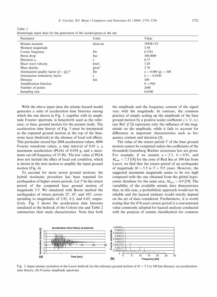
Table 1
Seismologic input data for the generation of the accelerogram at the site
Parameter Units Value
Seismic moment dyne cm 1995E+25
Moment magnitude 5.50
Corner frequency Hz 0.5781
Stress drop bar 100.0000
Duration td s 6.73
Shear wave velocity km/s 3.20
Mass density g/cm3 2.70
Attenuation quality factor Q ¼ Q0f n Hz n ¼ 0:800 Q0 ¼ 100
Attenuation inelasticity factor s k ¼ �0:0100
Distance km 100
Amplification function 0fiNO
Number of points 2048
Sampling rate 0.0100
S. Casciati, R.I. Borja / Computers and Structures 82 (2004) 1719–1736 1723
With the above input data the seismic hazard model
generates a suite of acceleration–time histories among
which the one shown in Fig. 3, together with its ampli-
tude Fourier spectrum, is henceforth used as the refer-
ence, or base, ground motion for the present study. The
acceleration–time history of Fig. 3 must be interpreted
as the expected ground motion at the top of the lime-
stone layer (bedrock) in the absence of local soil effects.
This particular record has 2048 acceleration values, 4096
Fourier transform values, a time interval of 0.01 s, a
maximum acceleration (PGA) of 0.034 g, and a maxi-
mum cut-off frequency of 25 Hz. The low value of PGA
does not include the effect of local soil condition, which
is shown in the next section to amplify the input ground
motion (Fig. 4).
To account for more severe ground motions, the
hybrid stochastic procedure has been repeated for
earthquakes of higher return periods. Let T be the return
period of the computed base ground motion of
magnitude 5.5. We simulated with Boore method the
earthquakes of return periods 2T , 4T , and 10T , corre-sponding to magnitudes of 5.85, 6.2, and 6.65, respec-
tively. Fig. 5 shows the acceleration time histories
simulated at the bedrock of the Colossi site and Table 2
summarizes their main characteristics. Note that both
Acceleration time history at bedrock
-4-3-2-101234
0 5 10 15 20 25
Time [sec]
Acc
eler
atio
n [c
m/s
ec2]
(a) (
Fig. 3. Input seismic excitation at the Luxor bedrock for the reference
time history; (b) Fourier amplitude spectrum.
the amplitude and the frequency content of the signal
vary with the magnitude. In contrast, the common
practice of simply scaling up the amplitude of the base
ground motion by a positive scalar coefficient k 2 ½1;1Þ(see Ref. [17]) represents only the influence of the mag-
nitude on the amplitude, while it fails to account for
differences in important characteristics such as fre-
quency content and duration [5].
The value of the return period T of the base ground
motion cannot be computed unless the coefficients of the
(bounded) Gutenberg–Richter recurrence law are given.
For example, if we assume a ¼ 2:3, b ¼ 0:91, and
Mmax ¼ 7:5 [18] for the zone of Red Sea at 100 km from
Luxor, we find that the return period of an earthquake
of magnitude M ¼ 5:5 is T ¼ 515 years. However, the
suggested maximum magnitude seems to be too high
compared with the one obtained from the global hypo-
center database for the same area, Mmax ¼ 4:9 [19]. The
variability of the available seismic data demonstrates
that, in this case, a probabilistic approach would not be
reliable and the hazard estimate would strictly depend
on the set of data considered. Furthermore, it is worth
noting that the 474-years return period is a conventional
value commonly adopted for hazard analyses conducted
with the purpose of seismic classification for common
00.00005
0.00010.00015
0.00020.00025
0.00030.00035
0.00040.00045
0 5 10 15 20 25 30Frequency [Hz]
Four
ier a
mpl
itude
b)
ground motion of M ¼ 5:5 at 100 km distance: (a) acceleration–

Fig. 5. Soil column model.
Acceleration time histories at bedrock
-4-3-2-101234
0 5 10 15 20 25
Time [sec]
Acc
eler
atio
n [c
m/s
ec2]
1T
Acceleration time histories at bedrock
-6
-4
-2
0
2
4
6
0 10 20 30 40 50
Time [sec]
Acc
eler
atio
n [c
m/s
ec2]
2T
Acceleration time histories at bedrock
-10
-5
0
5
10
0 10 20 30 40 50
Time [sec]
Acc
eler
atio
n [c
m/s
ec2]
4T
Acceleration time histories at bedrock
-15
-10
-5
0
5
10
15
0 10 20 30 40 50
Time [sec]
Acc
eler
atio
n [c
m/s
ec2]
10T
(a) (c)
(b) (d)
Fig. 4. Input seismic excitation at the Luxor bedrock for different return periods: (a) T ; (b) 2T ; (c) 4T and (d) 10T .
1724 S. Casciati, R.I. Borja / Computers and Structures 82 (2004) 1719–1736
buildings. In the case of an important structure, such as
a very ancient historical monument, a higher return
period is considered.
3. Local site response
The method described in the preceding section models
the reference ground motion for Luxor at the bedrock of
compacted limestone without taking into account the
local soil conditions. However, as seismic waves travel
Table 2
Acceleration–time histories at the bedrock
Return period Magnitude PGA [cm/s2]
T 5.5 3.307992
2T 5.85 5.084917
4T 6.2 )8.70287610T 6.65 12.340370
away from the source they reflect and refract on the
boundaries between geologic materials, and by the time
they reach the ground surface they propagate nearly in
the vertical direction. Hence, it is customary to analyze
the local site response using one-dimensional ground
response models. The term ‘1D response’ is not quite
precise as the word ‘dimension’ simply pertains to the
direction of wave propagation (vertical), but the body
waves still could have all three components of motion.
Several 1D site response models are available in the lit-
erature, including those based on an equivalent linear
analysis (e.g., SHAKE [20]) and those based on a fully
non-linear analysis (e.g., SPECTRA [6–9]). In the ab-
sence of precise information on the soil condition at the
site, we shall model the local site response in Luxor using
an equivalent linear analysis procedure, and specifically
using the computer program SHAKE91 [21].
SHAKE91 uses a vertical column model representing
the entire thickness of the soil deposit, in our case the 6
m-thick silt layer at the Collosi site. For a homogeneous
linearly elastic soil deposit, so-called transfer functions
in analytical form are available relating the input ground
motion at the base to the output ground motion at the
surface, and in this case it is not necessary to discretize
the soil layer. However, soils do experience some form of
Time [s] Number of points
3.81 2048
4.21 4096
6.53 4096
6.91 4096

S. Casciati, R.I. Borja / Computers and Structures 82 (2004) 1719–1736 1725
stiffness degradation depending upon the amount of
deformation, and thus the soil layer is commonly dis-
cretized into smaller segments so that the local degra-
dation effect can be captured accurately. For the silt
deposit at the site, we have divided the soil layer into six
sublayers as shown in Fig. 5. In view of keeping the same
vertical discretization for the 3D FE model of the soil
deposit, the upper two sublayers are 0.85 m thick
resulting in the statue being embedded 1.7 m into the
ground. The remaining four sublayers are 1.075 m thick
to achieve the total thickness of 6 m for the silt layer.
The properties of the silt layer at the Collosi site are
as follows: total mass density q ¼ 1400 kg/m3, unde-
graded Young’s modulus E ¼ 5 MPa, and Poisson’s
ratio m ¼ 0:33 [4]. The elastic shear modulus is then
determined as G ¼ 1:88 MPa, and the expected shear
wave velocity is estimated as vs ¼ 37 m/s. The value of
Poisson’s ratio, m ¼ 0:33, corresponds to a fully drained
condition. The Collosi site is located on the eastern side
of the river Nile where seasonal fluctuation of the
ground water table is common. Under a high water table
the silt could undergo undrained deformation and the
elastic Poisson’s ratio could reach a value close to 0.5.
Under this condition, G ¼ 1:67 MPa (for the same E)and vs ¼ 35 m/s. These values are not much different
from the drained case, and thus, provided the ground
motion is not strong enough to cause liquefaction, the
drainage condition is expected to have little effect on the
shear wave propagation. The very low values of G and vsfor the silt are characteristic of alluvial deposits, but they
could have also been influenced by soil disturbance
during testing (we have made no attempt to modify these
values to account for soil disturbance effects). In con-
trast, the limestone deposit is much stiffer, with a
Young’s modulus of E ¼ 12 GPa, an elastic Poisson’s
ratio of m ¼ 0:21, and a total mass density of q ¼ 2400
kg/m3 [4].
As the soil deforms in shear its overall shear stiffness
degrades and the hysteresis loop grows wider, resulting
0
0.2
0.4
0.6
0.8
1
Shear Strain (%)
G/G
max
0
5
10
15
20
25
30
Dam
ping
Rat
io (%
)
Shear ModulusDamping Ratio
0.
0.
0.
0.
0
G/G
max
(b)(a)
Fig. 6. Assumed modulus reduction and damping ratio curves for: (a
Idriss (1990), and Schnabel et al. (1972)].
in a softer response and increased damping. The dy-
namic soil properties are thus commonly expressed in
the form of shear modulus reduction G=Gmax and
damping ratio n curves, plotted as functions of the shear
strain. Unfortunately, such curves are not available for
the silt layer at the Collosi site. In this study we assume
the modulus reduction and damping ratio curves for
clay as described in [22,23] to represent the dynamic
properties of the silt layer, and those for rock as de-
scribed in [20] to represent the dynamic properties of the
limestone layer. These curves are shown in Fig. 6. Note
that the curves shown in Fig. 6 must be interpreted as
‘bands’ for purposes of statistical analysis [7], since
geotechnical data typically exhibit scattering due to ex-
pected variations in the soil properties and local condi-
tions. Thus, results of our site response analyses must
not be interpreted as blind predictions but only as rep-
resentative of those expected at the site.
Fig. 7 shows the amplification function (modulus of
the transfer function) for the base ground motion of
return period T ðM ¼ 5:5Þ, and the resulting accelera-
tion–time history of the output ground motion at the
surface assuming undrained condition for the silty layer.
The local soil condition has amplified the ground mo-
tion, specifically the PGA, by more than two times. The
peak amplification factor decreases with increasing
natural frequencies. The greatest amplification factor
occurs approximately at the lowest natural frequency
(also known as fundamental frequency), which depends
on the thickness of the soil deposit H and the shear wave
velocity vs. For the silt layer, this fundamental frequency
is estimated to be about x0 ¼ pvs=2H � 9 rad/s, or a
characteristic site period of about T0 ¼ 2p=x0 ¼ 0:7 s.
Downhole accelerograms were also generated by
SHAKE91 at the nodes of the soil column model to
better understand the nature of site amplification and
for subsequent use in the SFSI analysis.
The ground response analysis has been repeated
for the earthquakes of higher return periods and the
0
2
4
6
8
1
.0001 0.001 0.01 0.1 1Shear Strain (%)
00.5
11.5
2
2.5
3
3.5
4
4.55
Dam
ping
Rat
io (%
)
Shear ModulusDamping Ratio
) silt layer and for (b) limestone layer [After Sun et al. (1988),

0
5
10
15
20
25
0 5 10 15 20 25 30
Frequency [Hz]
Am
plifi
catio
n ra
tioLocal soil conditions amplification effect
-10
-5
0
5
10
0 10 20 30 40 50
Time [sec]
Acc
eler
atio
n [c
m/s
ec2]
Free FieldBedrock
(a) (b)
Fig. 7. Output ground motion at free surface for the reference ground motion of M ¼ 5:5 at 100 km distance: (a) amplification
function and (b) acceleration–time history.
Local soil conditions amplification effect, 1T
-10
-5
0
5
10
0 10 20 30 40 50
Time [sec]
Acc
eler
atio
n [c
m/s
ec2]
Free FieldBedrock
Local soil conditions amplification effect, 2T
-15
-10
-5
0
5
10
15
0 10 20 30 40 50
Time [sec]
Acc
eler
atio
n [c
m/s
ec2]
Free fieldBedrock
Local soil condition amplification effect, 10 T
-30
-20
-10
0
10
20
30
0 10 20 30 40 50
Time [sec]
Acc
eler
atio
n [c
m/s
ec2]
Free fieldBedrock
Local soil condition amplification effect, 4T
-20-15-10-505
1015
0 10 20 30 40 50
Time [sec]
Acc
eler
atio
n [c
m/s
ec2]
Free FieldBedrock
(a) (c)
(b) (d)
Fig. 8. Output ground motion at free surface for different return periods: (a) T ; (b) 2T ; (c) 4T and (d) 10T .
Table 3
Acceleration–time histories at free surface
Return period Magnitude PGA [cm/s2] Time [s] Amplification factor
T 5.5 8.428747 3.99 2.547995
2T 5.85 12.634280 6.51 2.484658
4T 6.2 )14.243150 6.14 1.636603
10T 6.65 )25.718880 6.29 )2.084126
1726 S. Casciati, R.I. Borja / Computers and Structures 82 (2004) 1719–1736
resulting acceleration–time histories at free surface are
summarized in Fig. 8. Table 3 shows how the frequency
content of the input ground motion influences the
amplification factor of its PGA value. In particular, the
maximum PGA amplification factor (2.55) occurs for
the input ground motion of lowest magnitude, while the
minimum (1.64) corresponds to the input ground motion
of return period 4T . Also note that the negative values of
acceleration become predominant for increasing return
periods. As a consequence of the local site condition, the
time at which the PGA value occurs has shifted; the
predominant period increases for the earthquakes of
lower return periods, T and 2T , while it decreases for theearthquakes of higher return periods, 4T and 10T .

S. Casciati, R.I. Borja / Computers and Structures 82 (2004) 1719–1736 1727
4. SFSI model and method of analysis
The results generated by the analysis of Section 3 are
free-field motions that would arise in the absence of the
structure. The actual motion at the base of the structure
may not necessarily be the same as the free-field motion
at the same soil level since it is known that the presence
of the structure contaminates the free-field motion. A
complete analysis must then include the SFSI effect,
where the letter ‘F’ has been explicitly inserted in the
acronym since the foundation, or base, interacts with
both the soil and the statue through their contact sur-
faces.
There are two commonly used methods of SFSI
analysis: multistep methods and direct methods [5].
Multistep methods use the principle of superposition to
combine the effects of kinematic and inertial interaction,
and are limited to the analysis of linear or equivalent
linear systems. Direct methods model the entire soil–
foundation–structure system in a single step and are
more robust than multistep methods, although they are
also more computationally demanding. Because of the
non-linearities arising from modeling the frictional links
at the base, we shall utilize the direct method of SFSI
analysis in this study.
Fig. 9 shows four views of the 3D finite element mesh
used to model the South Memnon Colossus including its
fractured base as well as the surrounding soil medium
(the North Colossus is not included in the model). De-
Fig. 9. Four views of the FE model for SFSI analysis: (a) front
tails of the statue itself are shown in the isometric view
of Fig. 10 and are discussed separately in the next sec-
tion. The structure is mounted on a flat soil region 6 m-
thick and supported by the limestone layer, herein
considered as the bedrock. Vertical walls on the sides of
the soil region form an elliptical boundary around the
structure. The soil region is discretized into six hori-
zontal sublayers such that the thicknesses of the sub-
layers are the same as those of the corresponding vertical
segments of the soil column model of Section 3. Essen-
tially, this is done to allow the specification of the pre-
viously calculated nodal free-field motions as essential
(or Dirichlet) boundary conditions around the soil re-
gion, as elaborated further below. Each horizontal slab
is then discretized further into elements across its
thickness, forming 3D brick finite elements whose
centroids are denoted by the symbol ‘·’ in Figs. 9 and
10. The limestone layer is not included in the FE model.
Each of the six horizontal soil slabs was assigned
values of the shear modulus G and damping ratio nconsistent with the effective shear strain level calculated
by SHAKE91 at each vertical segment of the soil col-
umn model. For example, the effective shear strain in
layer n is calculated by SHAKE91 as cn;eff ¼ Rccn;max,
where cn;max is the maximum shear strain in the com-
puted shear strain–time history for layer n, and
Rc � ðM � 1Þ=10 is a ratio that depends on the magni-
tude M of the earthquake. The nth soil slab in the 3D
mesh is then assigned values of G and n corresponding to
view; (b) isometric view; (c) plan view and (d) side view.

Fig. 10. Photogrammetric survey of the Southern Memnon Colossus: (a) front view; (b) lateral view and (c) isometric view of the FE
model.
Table 4
Degradation of the material properties of the soil deposit computed by SHAKE91 for the undrained condition
Accelerogram Equivalent
linear soil
properties
Layer
1 2 3 4 5 6
T G [MPa] 1.69 1.66 1.64 1.62 1.61 1.60
n 0.009 0.013 0.018 0.021 0.024 0.025
2T G [MPa] 1.66 1.62 1.60 1.59 1.58 1.53
n 0.012 0.021 0.025 0.027 0.030 0.036
4T G [MPa] 1.66 1.61 1.58 1.55 1.52 1.50
n 0.013 0.024 0.029 0.033 0.038 0.041
10T G [MPa] 1.63 1.54 1.49 1.46 1.40 1.36
n 0.021 0.035 0.043 0.047 0.056 0.062
1728 S. Casciati, R.I. Borja / Computers and Structures 82 (2004) 1719–1736
the effective shear strain level cn;eff . Table 4 shows the
values computed by SHAKE91 for the input ground
motions of different return periods assuming an un-
drained condition (Poisson’s ratio m close to 0.5). The
drained condition leads to a lesser degradation of the
shear modulus G, suggesting less damaging effects
compared to the undrained case.
We recall that SHAKE91 is an equivalent linear
analysis model, and even though it iterates to calculate
the effective strain level the converged solution is still
based on linear analysis. Our goal is to use the calculated
converged elastic soil properties to characterize the 3D
soil region. Thus, if the structure is removed and free-
field motions are applied on the boundaries of the 3D
soil model, then free-field motions will also be created in
the interior of the soil region. Therefore, in the presence
of the structure any computed deviation from the free-
field motion may be attributed directly to SFSI effects.
The FE method accepts the specification of the free-
field motion either in the form of a Dirichlet boundary
condition (displacement, velocity, acceleration) or in the
form of a natural (or Neumann) boundary condition
(equivalent nodal forces or surface tractions), but not
both. We have a well-defined limestone bedrock, and so
we have specified the free-field motion on the base of the
soil layer as a Dirichlet boundary condition. On the
vertical side walls of the soil region the free-field motion
may be applied either as a Neumann boundary condi-
tion in combination with the use of non-reflecting
boundaries [5] to absorb outgoing waves, or simply as a
Dirichlet boundary condition. The latter approach is
simpler and reasonably accurate provided the soil region
is large enough and the soil boundaries are far enough
from the structure. In this study we prescribe the free-
field motion as essential boundary conditions and
investigate the extent of the FE discretization on the
acuracy of the calculated SFSI responses following the
procedure described in Ref. [9].
Since the statue was pulled to the top of its base, the
foundation–structure system is essentially made up of

S. Casciati, R.I. Borja / Computers and Structures 82 (2004) 1719–1736 1729
two bodies in contact. The presence of a contact can serve
as a non-linear damper and thus must be included in the
modeling of SFSI. For purposes of specifying the contact,
we have assumed the sandstone blocks to be parts of
distinct deformable bodies and the contacting surfaces to
have a friction coefficient of l ¼ 0:5, which is typical for
sandstone [24–26]. In addition, we have also assumed the
base to interact with the surrounding soil, whose elements
form another deformable contact body. The contact
algorithm ensures that adjacent bodies do not overlap,
that there is no interaction between two non-contacting
bodies, and that if the bodies are in contact then the zones
of contact are governed by the laws of friction.
5. Procedure for 3D solid mesh generation
A photogrammetric representation of the statues has
been provided by the German Cultural Center, which is
currently working at the site for the rescue and resto-
ration of the remains of the destroyed temple. Fig. 10
shows front and lateral views of the South Memnon
Colossus images. The survey, which takes the form of an
image of JPG type in raster form, is not recent but is
sufficiently accurate. Polylines are superimposed to each
level line manually assigning the supporting points,
which can be achieved with the software Autocad14
simply by clicking on the mouse. A geo-reference of the
images, which pertains to the identification of common
points between two planar pictures representing the
front and lateral views of the statue, was necessary for
an accurate rendering of the 3D images of the solid.
The FE modeling of the structure was carried out
using the computer code MARC [27], which runs on
SUN workstations SUN Ultra1 and SUN-Blade 1000
under Solaris OS. The selected finite elements are iso-
parametric eight-noded bricks with tri-linear interpola-
tion functions. Initially, the coarse 3D FE mesh
proposed by Verdel [1,2] consisting of three parallel-
epipeds for the statue was reproduced in MARC. Then,
using the photogrammetric surveys, we developed a
more refined 3D FE mesh resembling the actual shape of
the statue. This was achieved by importing the afore-
mentioned photogrammetric information in the form of
polylines into the program MARC and centering the
image within the Verdel model. Then the nodes of the
external surface of the Verdel model were manually
brought to coincide with the points of the polylines
through the graphic interface MENTAT. This caused
some elements in the Verdel model to be removed and
many interior elements to be distorted. The resulting
refined mesh for the structure is composed of 1144 nodes
and 757 elements (in comparison, the original Verdel
description had 1330 nodes and 936 elements).
Severe element distortions could produce ill-condi-
tioning in the mathematical model. For example, some
Gauss integration points could fall outside the elements,
and some elements could be so distorted as to have as-
pect ratios well beyond the limits allowed for optimal
performance. The program automatically detects this
problem and allows the user to manually adjust the
nodes to correct the elements with severe geometric
distortions. It must be noted that for routine SFSI
analysis governed by masses and stiffnesses alone, the
need for such a very refined mesh for the structure may
not be that important. However, we are presently deal-
ing with a delicate and geometrically complex structure
that requires special attention to details. Consider, for
example, the fact that the statue’s weight was originally
estimated at 1070 metric tons by the coarser Verdel
model; our more refined rendering estimates the weight
of the statue to be 762 metric tons, for a difference of
almost 30%. Furthermore, we have identified the ab-
sence of material on the posterior part of the base which
could produce stress concentrations and instability
problems, but not captured by the coarser Verdel model.
Obviously, it also would be very difficult to predict the
stresses inside the statue itself if the FE mesh was not
properly refined. The final 3D FE mesh, including the
structure and the underlying soil deposit and shown in
Fig. 9, is composed of 3908 nodes, 2977 elements, and
9696 equations.
As for the material properties of the sandstone that
make up the Collosus, the material is assumed to be
isotropic linear elastic with a Young’s modulus ofeE ¼ 20 GPa, a Poisson’s ratio em ¼ 0:2, and a mass
density of eq ¼ 1800 kg/m3 [4]. A modal analysis of the
statue alone using these material properties produces the
first five frequencies of 12.8, 13.9, 34.7, 38.2, and 47.0 Hz
for the structure.
6. Non-linear transient dynamic analyses
Dynamic time-domain FE analyses were carried out
by applying the calculated free-field motions all along
the Dirichlet boundaries of the soil region. Starting from
a stationary initial condition (zero velocity), we pre-
scribed on the Dirichlet boundaries the free-field nodal
displacement–time histories obtained by twice integrat-
ing the acceleration–time histories computed by
SHAKE91. The remaining Neumann boundaries were
considered traction-free, including the horizontal
ground surface and the exposed surface of the monu-
ment. The shaking was applied along the shorter side of
the base (lateral or transverse direction with respect to
the statue).
The non-linearity in the analyses arises from the
contact and friction problems. Contact problems are
characterized by two important phenomena: gap open-
ing/closing and friction. The gap describes the contact
(gap closed) and separation (gap open) conditions of

1730 S. Casciati, R.I. Borja / Computers and Structures 82 (2004) 1719–1736
two objects (structures). Friction influences the interface
relations of the objects after they are in contact. The gap
condition is dependent on the movement (displacement)
of the objects, and friction is dependent on the contact
force as well as on the coefficient of Coulomb friction at
contact surfaces. The analysis involving gap and friction
was carried out incrementally. Iterations were done in
each load–time increment to stabilize the gap-friction
behavior. To advance the solution incrementally in time,
we employed a full Newton–Rapson iteration algorithm
based on a relative displacement tolerance of 0.1.
For time integration the second-order accurate
Newmark-beta algorithm with parameters c ¼ 1=2 and
b ¼ 1=4 was selected. For linear problems, this method
is unconditionally stable and exhibits no numerical
damping. However, instability can develop in the pres-
ence of non-linearities, which can be circumvented by
Fig. 11. Comparison of horizontal ground surface accelerations with
ratio¼ 0.499.
Fig. 12. Comparison of horizontal ground surface accelerations wi
(Poisson’s ratio¼ 0.499): (a) T ; (b) 2T ; (c) 4T and (d) 10T .
reducing the time step and/or adding (stiffness) damping.
To properly assign the time step, we first decided on the
frequencies that are important to the response of the
structure. In general, the time step should not exceed
10% of the period of the highest relevant frequency in
the structure, otherwise, large phase errors will occur.
The phenomenon usually associated with a time step
that is too large is strong oscillatory accelerations lead-
ing to numerical instability. To circumvent this problem
we have repeated the analysis with significantly different
time steps (1/5 and 1/10 of the original) and compared
the responses. After several trials, we fixed the time step
at Dt ¼ 0:01 s.
Damping represents the dissipation of energy in the
structural system. For the direct integration method, the
Rayleigh damping model was used in the analysis.
The global damping matrix was calculated as a linear
and without SFSI: (a) Poisson’s ratio¼ 0.33 and (b) Poisson’s
th and without SFSI for different earthquake return periods

Table 5
Acceleration–time histories near the base of the structure
Return period Magnitude PGA [cm/s2] Time [s] Amplification factor
T 5.5 16.694 9.5 1.975264
2T 5.85 25.425 8.68 2.012382
4T 6.2 )20.803 8.33 1.460562
10T 6.65 )38.166 12.1 1.483968
Soil surface nodes acceleration time histories
-20-15-10-505
101520
0 5 10 15 20 25
Time [sec]
Acc
eler
atio
n [c
m/s
ec2]
Soil surface nodes acceleration time histories
-15
-10
-5
0
5
10
15
0 5 10 15 20 25
Time [sec]
Acc
eler
atio
n [c
m/s
ec2]
Soil surface nodes acceleration time histories
-10
-5
0
5
10
0 5 10 15 20 25
Time [sec]A
ccel
erat
ion
[cm
/sec
2]
Soil surface nodes acceleration time histories
-8-6-4-202468
10
0 5 10 15 20 25
Time [sec]
Acc
eler
atio
n [c
m/s
ec2]
Distance:0m
Distance:4m
Distance:6m
Distance:10m
(a) (c)
(d)(b)
Fig. 13. Comparison of horizontal ground surface accelerations time histories at varying distances from the Colossus, for the ac-
celerogram of return period T : (a) 0 m; (b) 4 m; (c) 6 m and (d) 10 m away from the structure.
Table 6
Acceleration–time histories at varying distances from the
structure, for return period T
Distance [m] PGA [cm/s2] Time [s] Amplification
factor
0 16.694 9.5 2.162208
4 12.198 8.81 1.584156
6 8.129 8.81 1.055714
10 7.7 4.09 1
S. Casciati, R.I. Borja / Computers and Structures 82 (2004) 1719–1736 1731
combination of the element mass and stiffness matrices
through the equation
C ¼Xn
i¼1
aiM i
�þ bi
�þ ci
Dtp
�K i
�; ð5Þ
where C is the global damping matrix; n is the number
of elements in the mesh; M i is the mass matrix of the ithelement; K i is stiffness matrix; ai is the mass damping
coefficient; bi is the stiffness damping coefficient; ci is thenumerical damping coefficient; and Dt is the time
increment. The stiffness damping coefficients bi were
estimated from an empirical relationship with the
damping ratios ni as summarized in Table 4 for the soil
deposit. For the sandstone, bi was assumed to be about
2%. The mass matrix damping coefficient ai was kept
constant at 0.001.
The element stiffness matrix was formed using the
standard eight-point Gaussian integration rule, appro-
priate for eight-noded trilinear brick elements. Element
quantities such as stresses and strains were calculated at
each integration point. For the nearly incompressible
behavior the B-bar approach was used [28].
7. Results and discussions
To reduce the total number of possible combinations
of parameters, we first investigated the effect of drainage
condition in the silt layer. As mentioned earlier, this
entails using two values of Poisson’s ratio: m ¼ 0:33 for

Soil - Base Bottom Contact (nodes 2819-1531)
0
50
100
150
200
250
300
0 10 20 30 40
Time [sec]
Cum
ulat
ive
Plas
tic S
lip
[mm
]
1T2T4T10T
Soil - Base Bottom Contact (nodes 2928-1551)
0
50
100
150
200
250
300
0 10 20 30 40
Time [sec]
Cum
ulat
ive
Plas
tic S
lip
[mm
]
1T2T4T10T
Soil - Base Bottom Contact (nodes 2832-1980)
020406080
100120140
0 10 20 30 40
Time [sec]C
umul
ativ
e Pl
astic
Slip
[m
m]
1T2T4T10T
Soil - Base Bottom Contact (nodes 2795-1960)
020406080
100120140
0 10 20 30 40
Time [sec]
Cum
ulat
ive
Plas
tic S
lip
[mm
]
1T2T4T10T
Fig. 14. Cumulative plastic slip at the contact nodes between the statue and the base for different earthquake amplitudes.
Fig. 15. Cumulative plastic slip at the contact nodes between the base and the soil for different earthquake amplitudes.
1732 S. Casciati, R.I. Borja / Computers and Structures 82 (2004) 1719–1736
the drained case, and m ¼ 0:499 for the undrained case.
Applying the ground motion in the transverse direction
with respect to the statue, we compare in Fig. 11 the
effects of Poisson’s ratio on the horizontal ground sur-
face accelerations. To elucidate the comparison further,
the figure shows both the surface free-field motion and
the surface ground motion near the base of the statue.
The latter is expected to contain SFSI effects, which is
evident from the comparison of the two surface ground
motions. Note that the case where m ¼ 0:499 results in
stronger ground shaking. This is due in part to the fact
that for a fixed Young’s modulus E the elastic shear
modulus G decreases as the Poisson’s ratio m increases to0.5. However, introducing incompressible soil elements

Fig. 16. Von Mises stress distribution in the statue for accelerogram 10T .
S. Casciati, R.I. Borja / Computers and Structures 82 (2004) 1719–1736 1733
also enhances the sidesway mode but reduces the con-
tribution of the vertical and rocking modes (they be-
come higher frequency modes due to the increased bulk
stiffness), thus amplifying the horizontal ground motion.
For this reason, we shall focus the analysis on the more
critical case of undrained deformation, and hence use
m ¼ 0:499 for the soil deposit throughout.
Fig. 12 compares the free field motion and the surface
ground motion near the base of the statue for earth-
quakes of different return periods. The maximum
absolute values of acceleration increase in the proximity
of the statue. The amplification factors of the PGA of
the free field motions are summarized in Table 5. The
PGA is amplified by a factor of about two for the ac-
celerograms of return periods T and 2T , and by a factor
of about 1.5 for the accelerograms of return periods 4Tand 10T . Note that the maximum absolute value of
ground motion acceleration corresponding to a return
period 2T is higher than the one corresponding to a
return period of 4T near the base of the statue. Also the
predominant period of the ground motions increases in
the vicinity of the structure.
Next, we investigate the extent of discretized zone on
the propagation of scattered waves induced by SFSI
effects. Fig. 13 and Table 6 show the surface ground
motions at points 0, 4, 6, and 10 m away from the side of
the base of the statue, for the accelerograms of return
period T . The maximum absolute values of acceleration
and the corresponding predominant periods decrease
with increasing distance from the statue. The surface
ground motion with SFSI approaches the free field
ground motion near the vertical side boundaries of the
soil, as expected.
To better understand the influence of ground shaking
on the interaction between the individual components of
the soil–foundation–structure system, we show in Figs.
14 and 15 the cumulative plastic slip at the bottom of the
base relative to the underlying foundation soil, and the
cumulative plastic slip of the bottom of the statue rela-
tive to its base, respectively, as functions of time and
earthquake amplitude. These plastic slips represent the
cumulative slips at the contact nodes obtained by sum-
ming the absolute values of the incremental plastic slips
experienced throughout the duration of the analysis.
Note that the cumulative plastic slip is not the final
distance that one block moves relative to the adjacent
block. If at the nth time increment Dt the incremental
plastic slip between the two contact nodes is di ¼ kDd ik,then the cumulative plastic slip is
Pdi. In other words,
even if the two blocks returned to their original positions
the cumulative plastic slip would still be greater than
zero because it represents the total excursion or distance

1734 S. Casciati, R.I. Borja / Computers and Structures 82 (2004) 1719–1736
that the two blocks have traveled relative to each other.
Thus, the cumulative plastic slips monotonically in-
crease with time.
The cumulative plastic slip values were sampled at
the contact nodes located at the corners of the base
bottom and statue bottom, respectively, where the
stresses are expected to be high. Note that the cumula-
tive plastic slips reach higher values at the contact nodes
in the rear end of the structure, which supports most of
the weight of the statue. The cumulative slip curves
corresponding to earthquakes with return periods 2Tand 4T are quite similar to each other, while the ones
corresponding to return periods of T and 10T represent
lower and upper bounds to the cumulative slips,
respectively. In general, the plastic slips computed at the
contact between the bottom of the base and the under-
lying soil are greater than those computed at the contact
between the bottom of the statue and the top of the base.
Fig. 17. Details of the Von Mises stress distribution for accelerogram 1
bottom and (d) soil foundation top.
Finally, Figs. 16 and 17 identify the probable zones
of stress concentration in the statue, the supporting
base, and the underlying soil foundation during the
period of most intense ground shaking for an earth-
quake of return period 10T . The figures plot the con-
tours of Von Mises stresses (defined asffiffiffiffiffiffiffiffi3=2
pksk, where s
is the deviatoric component of the Cauchy stress tensor
r and the symbol k � k denotes a tensor norm), a stress
measure commonly used to describe the level of shearing
in a continuum. As shown in the figures the Von Mises
stress values are higher at the contact between the top of
the base and the bottom of the statue than at the contact
between the bottom of the base and the underlying
foundation soil, even though the cumulative plastic slips
are lower for the former than for the latter. Represen-
tations such as these are useful for designing possible
retrofit measures for the monument since they identify
regions where the stress demands are likely to be high.
0T , at various locations: (a) statue bottom; (b) base top; (c) base

S. Casciati, R.I. Borja / Computers and Structures 82 (2004) 1719–1736 1735
8. Summary and conclusions
We have presented a methodology for non-linear
dynamic SFSI analysis of an important landmark, the
South Memnon Colossus in Luxor, Egypt, as it responds
to artificially generated earthquakes of different return
periods. The methodology involves a consistent frame-
work for seismic hazard analysis applicable to important
structures located in developing countries where data are
scarce if not completely lacking. Apart from our inter-
ests in quantifying the seismic response of this particular
structure for educational purposes as well as for inves-
tigating possible retrofit measures for the fractured
foundation base, we have carried out these detailed
studies in an attempt to combine, in a systematic fash-
ion, different aspects of earthquake engineering analysis
with available analytical and computational modeling
tools. The modeling included the use of a hybrid sto-
chastic approach for generating synthetic earthquakes of
different return periods based on the seismicity of the
region, the analysis of the local site response based on
available soils data, and the modeling of the SFSI effects
using three-dimensional time-domain non-linear FE
analysis. The studies demonstrate how different solution
methodologies may be used in tandem to analyze com-
plex earthquake engineering problems.
Acknowledgements
Financial support for this research was provided in
part by National Science Foundation under contract no.
CMS-02-01317 through the direction of Dr. Clifford S.
Astill. Funding for the first author was provided by a
research assistantship from the John A. Blume Earth-
quake Engineering Center. The authors are grateful to
Dr. Alberto Marcellini of University of Pavia for assis-
tance with the generation of the earthquake source
model for Luxor; to Drs. David Pollard and Atilla
Aydin of Stanford University for providing some insight
into the mechanical properties of fault zones; and to an
anonymous reviewer for his/her constructive review.
References
[1] Verdel T. G�eotechnique et monuments historiques,
m�ethodes de mod�elisation appliqu�ees �a des cas �egyptiens
[in French]. Phd thesis, INPL-Ecole des Mines, Nancy,
France; 1993.
[2] Verdel T. Stability of the Colossus of Memnon: prelimin-
ary geotechnical study. Nancy, France: Ecoles des Mines;
1991.
[3] El Shabrawi A, Verdel T. The seismic risk on ancient
masonry structures by the use of the distinct element
method. Unrefereed paper; 1993.
[4] Casciati S. Analisi di pericolosit�a, fragilit�a sismica ed
ipotesi di adeguamento per uno dei colossi di Memmone
[in Italian]. Msd thesis, Department of Structural Mechan-
ics, University of Pavia, Italy 2001.
[5] Kramer SL. Geotechnical earthquake engineering. Engle-
wood-Cliffs, NJ: Prentice-Hall; 1996.
[6] Borja RI, Duvernay BG, Lin CH. Ground response in
lotung: total stress analysis and parametric studies. J
Geotechn Geoenviron Eng ASCE 2002;128:54–63.
[7] Borja RI, Lin CH, Sama KM, Masada GM. Modelling
non-linear ground response of non-liquefiable soils. Earth-
quake Eng Struct Dyn 2000;29:63–83.
[8] Borja RI, Chao HY, Mont�ans FJ, Lin CH. Nonlinear
ground response at Lotung LSST site. J Geotechn Geoen-
viron Eng ASCE 1999;125:187–97.
[9] Borja RI, Chao HY, Mont�ans FJ, Lin CH. SSI effects on
ground motion at Lotung LSST site. J Geotechn Geoen-
viron Eng ASCE 1999;125:760–70.
[10] Said R. The geology of Egypt. Brookfield, Rotterdam:
A.A. Balkema; 1990.
[11] Casciati F, Casciati S, Marcellini A. PGA and structural
dynamics input motion at a given site. J Earthquake Eng
Eng Vibrat 2003;2:25–33.
[12] Boore D. Stochastic simulation of high-frequency
ground motions based on seismological model of the
radiated spectra. Bull Seismol Soc Am 1983;73:1865–
94.
[13] Brune J. Tectonic stress and the spectra of seismic shear
waves from earthquakes. J Geophys Res 1970;75:4997–
5009.
[14] Brune J. Correction. J Geophys Res 1971;76:5002.
[15] Saragoni R, Hart G. Simulation of artificial earthquakes.
Earthquake Eng Struct Dyn 1974;2:249–67.
[16] Marcellini A, Daminelli R, Franceschina G, Pagani M.
Regional and local seismic hazard assessment. Soil Dyn
Earthquake Eng 2001;21:415–29.
[17] Vamvatsikos D, Cornell CA. Incremental dynamic analy-
sis. Earthquake Eng Struct Dyn 2002;31:491–514.
[18] Riad S, Yousef M. Earthquake hazard assessment in the
southern part of the western desert of Egypt. Report
submitted to the National Authority for Remote Sens-
ing and Space Sciences. Center of Studies and Research
for the South Valley Development Assuit University;
1999.
[19] US Geological Survey. Global hypocenter data base––
version 3. United States Geological Survey, National
Earthquake Information Center; 1994.
[20] Schnabel PB, Lysmer J, Seed, HB. SHAKE––a computer
program for earthquake response analysis of horizontally
layered sites. EERC Report No. 72-12, Earthquake Engi-
neering Research Center, University of California at
Berkeley, CA; December 1972.
[21] Idriss I, Sun JI. SHAKE91––a computer program for
conducting equivalent linear seismic response analyses of
horizontally layered soil deposits. Center for Geotechnical
Modeling, University of California at Davis, CA; Novem-
ber 1992.
[22] Sun JI, Golesorkhi R, Seed HB. Dynamic moduli and
damping ratios for cohesive soils. Report No. UCB/
EERC-88/15, Earthquake Engineering Research Center,
University of California at Berkeley, CA; 1988.

1736 S. Casciati, R.I. Borja / Computers and Structures 82 (2004) 1719–1736
[23] Idriss I. Response of soft soil sites during earthquakes. In:
Proceedings of the Memorial Symposium to Honor Pro-
fessor Harry Bolton Seed, Berkeley, CA, vol. II; May 1990.
[24] Barton N. Review of a new shear-strength criterion for
rock joints. Eng Geol 1973;7:287–332.
[25] Byerlee J. Friction of rocks. Pure Appl Geophys 1978;116:
615–26.
[26] Dieterich JH, Kilgore BD. Direct observation of frictional
contacts: new insights for state-dependent properties. Pure
Appl Geophys 1994;143:283–302.
[27] MARC vol. A: Theory and user information, version 7.3;
August 1998.
[28] Hughes TJR. The finite element method. Englewood-Cliffs,
NJ: Prentice-Hall; 1987.
Recommended