Durham Research Online

Deposited in DRO:

07 April 2008

Version of attached �le:

Accepted Version

Peer-review status of attached �le:

Peer-reviewed

Citation for published item:

Woodro�e, S. A. and Horton, B. P. (2005) 'Holocene sea-level changes in the Indo-Paci�c.', Journal of Asianearth sciences., 25 (1). pp. 29-43.

Further information on publisher's website:

http://dx.doi.org/10.1016/j.jseaes.2004.01.009

Publisher's copyright statement:

Additional information:

Use policy

The full-text may be used and/or reproduced, and given to third parties in any format or medium, without prior permission or charge, forpersonal research or study, educational, or not-for-pro�t purposes provided that:

• a full bibliographic reference is made to the original source

• a link is made to the metadata record in DRO

• the full-text is not changed in any way

The full-text must not be sold in any format or medium without the formal permission of the copyright holders.

Please consult the full DRO policy for further details.

Durham University Library, Stockton Road, Durham DH1 3LY, United KingdomTel : +44 (0)191 334 3042 | Fax : +44 (0)191 334 2971

http://dro-test.dur.ac.uk

1

1

Holocene sea-level changes in the Indo-Pacific

S. A. WOODROFFE*. Environmental Research Centre, Department of Geography, University of

Durham, South Road, Durham, DH1 3LE, UK. Tel: 0191 334 1860 Fax: 0191 334 1801. E-mail:

s.a.woodroffe@durham.ac.uk.

B. P. HORTON. Environmental Research Centre, Department of Geography, University of

Durham, South Road, Durham, DH1 3LE, UK.

* - Correspondent

Abstract

Holocene sea-level reconstructions exist from many locations in the Indo-Pacific region. Despite

being a large geographical region, the nature of Holocene sea-level change is broadly similar in all

locations. Differences do exist however, in the timing and magnitude of the Mid-Holocene High

Stand (MHHS) and the nature of late Holocene sea level fall across the region. When the Indo-

Pacific is subdivided into smaller regions, these discrepancies do not disappear, and in some

cases the discrepancies are large within a single coastline.

It is clear from this analysis that the fundamental criteria to produce accurate local relative sea-

level curves are hardly ever met. There are serious problems associated with the correct

interpretation of sea-level indicators and their relationship to mean sea level, and with the quality of

age determinations. A consistent methodology throughout the Indo-Pacific for the analysis of sea

level data is lacking. Future sea-level analysis from far field locations must involve the application

of a consistent methodology in order to allow meaningful comparison between studies. This

should help to resolve the ongoing debate about the magnitude and timing of the Mid-Holocene

High Stand, and the nature of late Holocene sea-level fall across the region.

2

2

1. Introduction

Oscillations between glacial and interglacial climate conditions during the Quaternary have been

characterized by the transfer of immense volumes of water between ice sheets and the oceans

(e.g., Broecker and Denton, 1989; Alley and Clark, 1999; McManus et al., 1999; Lambeck et al.,

2002). Since the latest of these oscillations, the Last Glacial Maximum (between about 30,000 and

19,000 years ago), approximately 50 x106 km3 of ice has melted from the land-based ice sheets,

raising global sea level in regions distant from the major glaciation centres (far-field locations) by

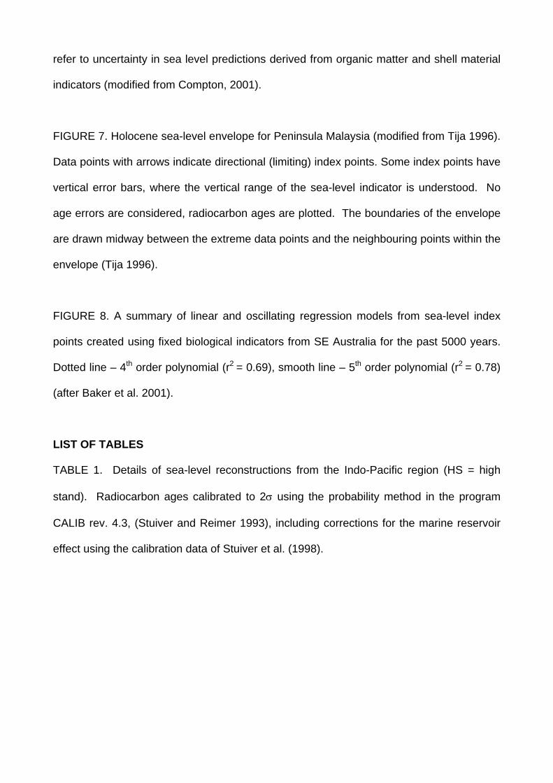
about 130 metres (Fig 1) (e.g. Lambeck et al., 2002). In contrast, relative sea levels have dropped

by many hundreds of metres in regions once covered by the major ice sheets (near- and

intermediate-field locations) as a consequence of the isostatic ‘rebound' of the solid Earth following

the melting of land-based ice (Shennan and Horton, 2002). Such rapid changes in sea level are

part of a complex pattern of interactions among the oceans, ice sheets and solid earth, all of which

have different response timescales. Geographical variability in Holocene sea-level change is well

illustrated by Pirazzoli’s (1991) atlas of sea-level curves and by geophysical model predictions

(e.g., Clark et al., 1978; Peltier, 2002; Shennan, et al., 2002; Lambeck et al., 2003; Mitrovicia,

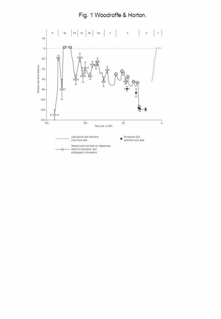
2003). Clark et al. (1978) identified six different sea-level patterns which reflect a range of sea-

level histories recorded at coasts which have emerged, submerged, or are in transitional areas and

record a combination of both uplift and subsidence (Fig 2). Although much contemporary research

(e.g., Shennan and Horton, 2002) to test such theoretically derived models has focused on data

sets from near- and intermediate-field locations (Zones I –II), it is widely recognised that ‘far-field

locations’ (Zones III – VI) provide the best possible estimate of the ‘eustatic function’ (Clark et al.,

1978; Yokoyama et al., 2000; Peltier, 2002). Consequently, model derived reconstructions are

increasingly recognising the importance of these areas to constrain and test their earth-ice models

(eg. Fleming et al. 1998).

2. Past sea-level changes

At their simplest changes in relative sea level (RSL) are a product of changes in oceanic and crustal

variables. A change in relative sea level at any time or location is dependent upon a combination of

sea surface level changes, any isostatic or tectonic changes, and local coastal processes.

The ocean, or eustatic level is influenced by three main groups of factors; the water volume in the

oceans; the volume of the ocean basins; and the distribution of the water. The water in the ocean

and the volume of glacial ice on land are in balance; when one increases the other decreases.

This is known as glacial eustasy (first proposed by Suess, 1888). The ocean volume is also

modulated by a number of other factors, such as the addition of juvenile water, storage of water in

3

3

sediments, variations in the main hydrologic cycle changing continental lake volumes, cloudiness,

and the evaporation/precipitation balance. A factor of high significance is the steric

expansion/contraction of the water column. These changes are driven by temperature and, to a

lesser degree, salinity. Steric changes are advocated as one of the most important factors in future

sea-level estimates (e.g., Houghton, 2001). The basins of the oceans may change their level by

crustal movements so that they increase and decrease in total volume. This is tectono-eustasy. In

reality, this is merely deformation of the hypsographic curve, and is a slow process, which may

only change sea level by 0.06 mm yr-1 (Mörner, 1996).

The ocean water level also changes as the result of the global distribution of oceanic water. This is

known as geoidal eustasy (Mörner, 1976). The earth is not spherical, but broadly flattened at the

poles and bulging at the equator and the ocean surface does not parallel that of the earth. Present

geodetic sea level varies with respect to the earths centre by as much as 180 m. The geoid relief

does not remain stable with time; it deforms vertically as well as horizontally. During the Last

Glacial Maximum, the weight of continental ice sheets caused downward deformation of the crust,

forcing sublithospheric flow away from the centres of load. A low latitude gravitational anomaly

developed creating a high in the oceanic geoid. During the last glacial deglaciation, the continents

viscoelastically rebounded causing the gravity anomaly to decay and the oceanic geoid to migrate

from lower to higher latitudes. This geoidal process is called equatorial ocean syphoning

(Mitrovica and Peltier, 1991). The relative sea level (RSL) effects of equatorial ocean syphoning

are only seen in the late Holocene (last 3000 years), where in low latitudes oceanic islands such

as the Cocos Keeling Islands have experienced a fall in RSL (Woodroffe and McLean 1990).

Global glacial isostatic adjustment is the process whereby the Earth's shape and gravitational field

are modified in response to the large scale changes in surface mass load that have occurred due

to the glaciation and deglaciation of the planetary surface (according to Archimedes principle). As

shown by Daly (1934), the development of an ice sheet will result in subsidence beneath the ice

mass (glacio isostasy), when deeper material flows away and a peripheral bulge is built around the

ice margin. When the ice sheet melts, unloading occurs, resulting in uplift beneath the melted ice

at rates which may locally reach 50 to 100 mm yr-1 (Pirazzoli, 2000); the marginal rim will

consequently tend to subside and move towards the centre of the vanishing load. Furthermore,

during deglaciation meltwater from the ice sheets produces a considerable load (of the order of

100 t m2 for a sea-level rise of 100 m (Lambeck et al. 2002)) on the ocean floors so that the sea

floor subsides (hydro-isostasy). Interest in studying the response of the planet to these Quaternary

glacial cycles derives primarily from the fact that the geological, geophysical and astronomical data

which record them are of such high quality. Furthermore, these data are almost uniquely capable

of providing firm constraints upon the viscoelastic properties of the "solid" interior of the earth and

4

4

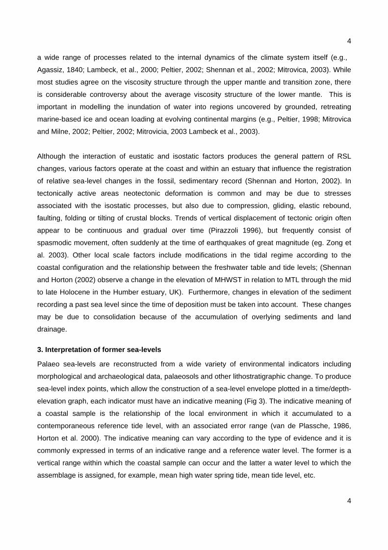
a wide range of processes related to the internal dynamics of the climate system itself (e.g.,

Agassiz, 1840; Lambeck, et al., 2000; Peltier, 2002; Shennan et al., 2002; Mitrovica, 2003). While

most studies agree on the viscosity structure through the upper mantle and transition zone, there

is considerable controversy about the average viscosity structure of the lower mantle. This is

important in modelling the inundation of water into regions uncovered by grounded, retreating

marine-based ice and ocean loading at evolving continental margins (e.g., Peltier, 1998; Mitrovica

and Milne, 2002; Peltier, 2002; Mitrovicia, 2003 Lambeck et al., 2003).

Although the interaction of eustatic and isostatic factors produces the general pattern of RSL

changes, various factors operate at the coast and within an estuary that influence the registration

of relative sea-level changes in the fossil, sedimentary record (Shennan and Horton, 2002). In

tectonically active areas neotectonic deformation is common and may be due to stresses

associated with the isostatic processes, but also due to compression, gliding, elastic rebound,

faulting, folding or tilting of crustal blocks. Trends of vertical displacement of tectonic origin often

appear to be continuous and gradual over time (Pirazzoli 1996), but frequently consist of

spasmodic movement, often suddenly at the time of earthquakes of great magnitude (eg. Zong et

al. 2003). Other local scale factors include modifications in the tidal regime according to the

coastal configuration and the relationship between the freshwater table and tide levels; (Shennan

and Horton (2002) observe a change in the elevation of MHWST in relation to MTL through the mid

to late Holocene in the Humber estuary, UK). Furthermore, changes in elevation of the sediment

recording a past sea level since the time of deposition must be taken into account. These changes

may be due to consolidation because of the accumulation of overlying sediments and land

drainage.

3. Interpretation of former sea-levels

Palaeo sea-levels are reconstructed from a wide variety of environmental indicators including

morphological and archaeological data, palaeosols and other lithostratigraphic change. To produce

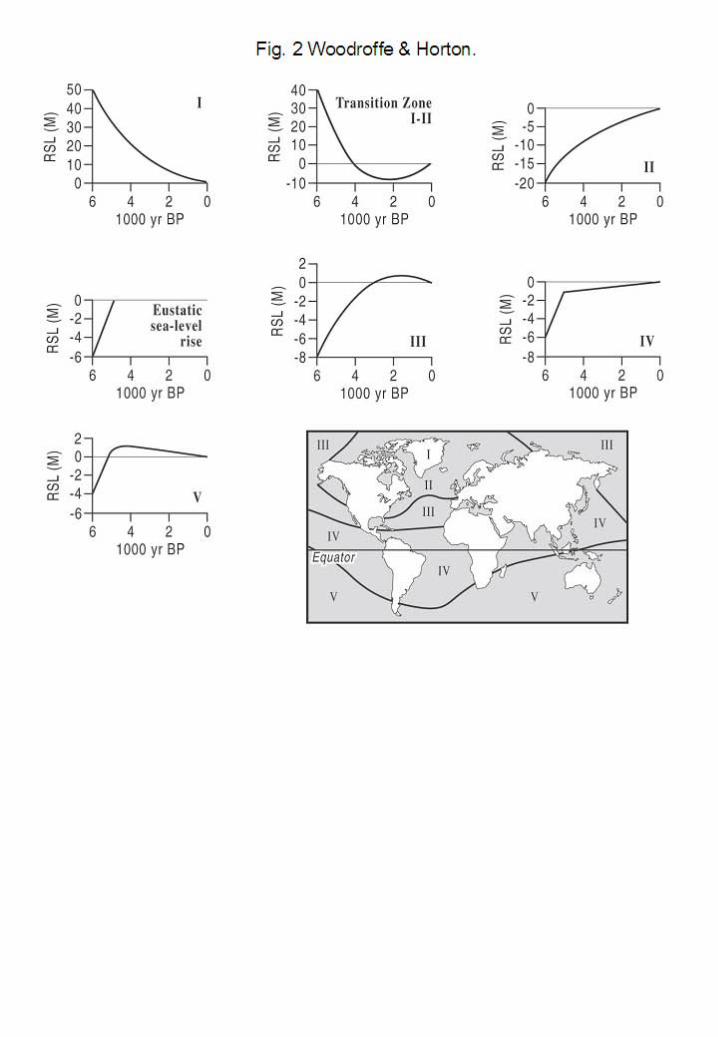
sea-level index points, which allow the construction of a sea-level envelope plotted in a time/depth-

elevation graph, each indicator must have an indicative meaning (Fig 3). The indicative meaning of

a coastal sample is the relationship of the local environment in which it accumulated to a

contemporaneous reference tide level, with an associated error range (van de Plassche, 1986,

Horton et al. 2000). The indicative meaning can vary according to the type of evidence and it is

commonly expressed in terms of an indicative range and a reference water level. The former is a

vertical range within which the coastal sample can occur and the latter a water level to which the

assemblage is assigned, for example, mean high water spring tide, mean tide level, etc.

5

5

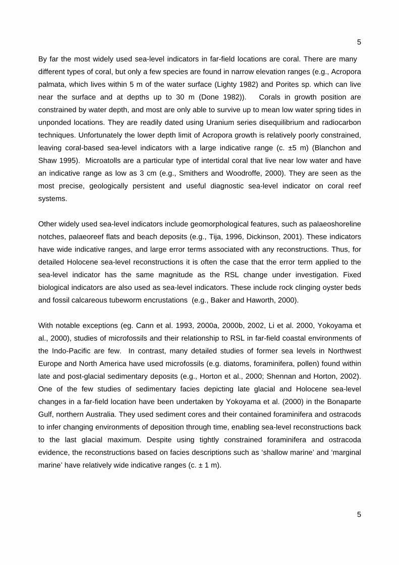
By far the most widely used sea-level indicators in far-field locations are coral. There are many

different types of coral, but only a few species are found in narrow elevation ranges (e.g., Acropora

palmata, which lives within 5 m of the water surface (Lighty 1982) and Porites sp. which can live

near the surface and at depths up to 30 m (Done 1982)). Corals in growth position are

constrained by water depth, and most are only able to survive up to mean low water spring tides in

unponded locations. They are readily dated using Uranium series disequilibrium and radiocarbon

techniques. Unfortunately the lower depth limit of Acropora growth is relatively poorly constrained,

leaving coral-based sea-level indicators with a large indicative range (c. ±5 m) (Blanchon and

Shaw 1995). Microatolls are a particular type of intertidal coral that live near low water and have

an indicative range as low as 3 cm (e.g., Smithers and Woodroffe, 2000). They are seen as the

most precise, geologically persistent and useful diagnostic sea-level indicator on coral reef

systems.

Other widely used sea-level indicators include geomorphological features, such as palaeoshoreline

notches, palaeoreef flats and beach deposits (e.g., Tija, 1996, Dickinson, 2001). These indicators

have wide indicative ranges, and large error terms associated with any reconstructions. Thus, for

detailed Holocene sea-level reconstructions it is often the case that the error term applied to the

sea-level indicator has the same magnitude as the RSL change under investigation. Fixed

biological indicators are also used as sea-level indicators. These include rock clinging oyster beds

and fossil calcareous tubeworm encrustations (e.g., Baker and Haworth, 2000).

With notable exceptions (eg. Cann et al. 1993, 2000a, 2000b, 2002, Li et al. 2000, Yokoyama et

al., 2000), studies of microfossils and their relationship to RSL in far-field coastal environments of

the Indo-Pacific are few. In contrast, many detailed studies of former sea levels in Northwest

Europe and North America have used microfossils (e.g. diatoms, foraminifera, pollen) found within

late and post-glacial sedimentary deposits (e.g., Horton et al., 2000; Shennan and Horton, 2002).

One of the few studies of sedimentary facies depicting late glacial and Holocene sea-level

changes in a far-field location have been undertaken by Yokoyama et al. (2000) in the Bonaparte

Gulf, northern Australia. They used sediment cores and their contained foraminifera and ostracods

to infer changing environments of deposition through time, enabling sea-level reconstructions back

to the last glacial maximum. Despite using tightly constrained foraminifera and ostracoda

evidence, the reconstructions based on facies descriptions such as ‘shallow marine’ and ‘marginal

marine’ have relatively wide indicative ranges (c. ± 1 m).

6

6

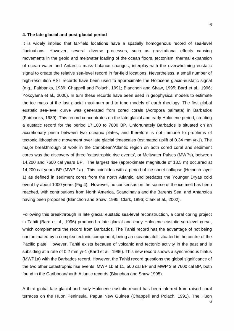
4. The late glacial and post-glacial period

It is widely implied that far-field locations have a spatially homogenous record of sea-level

fluctuations. However, several diverse processes, such as gravitational effects causing

movements in the geoid and meltwater loading of the ocean floors, tectonism, thermal expansion

of ocean water and Antarctic mass balance changes, interplay with the overwhelming eustatic

signal to create the relative sea-level record in far-field locations. Nevertheless, a small number of

high-resolution RSL records have been used to approximate the Holocene glacio-eustatic signal

(e.g., Fairbanks, 1989; Chappell and Polach, 1991; Blanchon and Shaw, 1995; Bard et al., 1996;

Yokoyama et al., 2000). In turn these records have been used in geophysical models to estimate

the ice mass at the last glacial maximum and to tune models of earth rheology. The first global

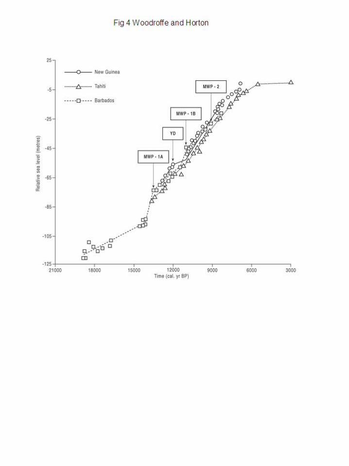
eustatic sea-level curve was generated from cored corals (Acropora palmata) in Barbados

(Fairbanks, 1989). This record concentrates on the late glacial and early Holocene period, creating

a eustatic record for the period 17,100 to 7800 BP. Unfortunately Barbados is situated on an

accretionary prism between two oceanic plates, and therefore is not immune to problems of

tectonic lithospheric movement over late glacial timescales (estimated uplift of 0.34 mm yr-1). The

major breakthrough of work in the Caribbean/Atlantic region on both cored coral and sediment

cores was the discovery of three ‘catastrophic rise events’, or Meltwater Pulses (MWPs), between

14,200 and 7600 cal years BP. The largest rise (approximate magnitude of 13.5 m) occurred at

14,200 cal years BP (MWP 1a). This coincides with a period of ice sheet collapse (Heinrich layer

1) as defined in sediment cores from the north Atlantic, and predates the Younger Dryas cold

event by about 1000 years (Fig 4). However, no consensus on the source of the ice melt has been

reached, with contributions from North America, Scandinavia and the Barents Sea, and Antarctica

having been proposed (Blanchon and Shaw, 1995; Clark, 1996; Clark et al., 2002).

Following this breakthrough in late glacial eustatic sea-level reconstruction, a coral coring project

in Tahiti (Bard et al., 1996) produced a late glacial and early Holocene eustatic sea-level curve,

which complements the record from Barbados. The Tahiti record has the advantage of not being

contaminated by a complex tectonic component, being an oceanic atoll situated in the centre of the

Pacific plate. However, Tahiti exists because of volcanic and tectonic activity in the past and is

subsiding at a rate of 0.2 mm yr-1 (Bard et al., 1996). This new record shows a synchronous hiatus

(MWP1a) with the Barbados record. However, the Tahiti record questions the global significance of

the two other catastrophic rise events, MWP 1b at 11, 500 cal BP and MWP 2 at 7600 cal BP, both

found in the Caribbean/north Atlantic records (Blanchon and Shaw 1995).

A third global late glacial and early Holocene eustatic record has been inferred from raised coral

terraces on the Huon Peninsula, Papua New Guinea (Chappell and Polach, 1991). The Huon

7

7

Peninsula is tectonically active, being close to the edge of the Philippine plate, and is

experiencing uplift at a rate of ~1.9 mm yr-1. By decoupling the tectonic and eustatic elements of

RSL history in the area, a global eustatic sea-level curve has been developed. However, aseismic

uplift on the Huon Peninsula is episodic, dominated by isolated, metre scale events with 1000 year

reoccurrence intervals, which contaminates the record with a complex tectonic component.

The nature of mid to late Holocene global eustatic sea-level change is less well documented.

Indeed Nunn (1998) refers to the last millennium as a ‘1000-year hiatus’ in sea-level research of

the Pacific (Long, 2000). Emphasis switches from aiming to produce a globally valid eustatic sea-

level curve to understanding local and regional influences on RSL reconstructions. Therefore, for

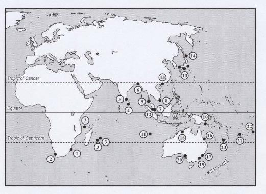
the purposes of this review we have split the Indo-Pacific into six sub-regions; Southwest Indian

Ocean, Northern Indian Ocean, Southeast Asia, Northern Asia, Australia and Pacific Ocean (Fig 5

and Table 1).

4.1 Southwest Indian Ocean

The southwest Indian Ocean includes the continental coastline of southeast Africa, the micro

continent of Madagascar, and several oceanic atolls including Mayotte, Reunion, Mauritius and the

Seychelles. Field observations in these locations have utilized a range of geomorphological and

biological indicators including beachrock, oyster beds, coral reefs and marine shells to reconstruct

mid to late Holocene changes in RSL (e.g., Ramsay, 1995; Colonna et al., 1996; Camoin et al.,

1997; Compton, 2001; Ramsay and Cooper, 2002). The southwest Indian Ocean is tectonically

stable, being situated towards the centre of the African plate and, therefore, observations from

these locations should yield important information regarding glacio-eustasy and hydro-isostasy.

Studies of Holocene sea-level change in South Africa have relied mainly on radiocarbon dating of

fossil beachrock. Beachrock is a reliable sea-level indicator, assuming that the skeletal carbonate

content is entirely contemporary. It forms today at the freshwater/saltwater interface at 0.1 - 0.2 m

below mean sea level (Ramsay and Cooper, 2002). Ramsay (1995) produced a 9000 year record

showing early Holocene RSL rise to a mid-Holocene high stand of +3.5 m at 4650 14C yrs BP with

RSL subsequently falling below present levels, but also shows a secondary high stand at 1610 14C

yrs BP (+ 1.5 m) before mean sea level is attained at 900 14C yrs BP. The sea-level observations

are taken from a 180 km long stretch of coastline in eastern South Africa, thus reflecting regional

RSL influences. However, the sea-level index points are not corrected for their indicative meaning.

For example, some index points from the early Holocene use dated wood, which should be treated

as limiting points, that is RSL must have been at or below the level at which they are found,

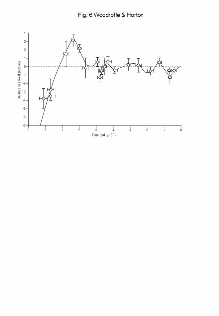
however they are included in the curve as standard index points. A second investigation in South

Africa has concentrated on a saltmarsh lagoon on the southwest coast (Compton, 2001). This

8

8

lagoon is situated on the Atlantic coast, where tectonic activity has occurred through the

Holocene, and the RSL history reflects more Atlantic rather than Indian Ocean processes. The

RSL record, derived from radiocarbon dated saltmarsh peats, agrees with Ramsay’s two mid-late

Holocene high stands theory, and uses potentially more precise indicators (Fig 6). However, the

indicative meaning of each indicator is not explicitly stated and all late Holocene sea-level

fluctuations after the initial mid-Holocene peak of +3 m are within the elevation ranges of the

indicators.

Holocene sea-level changes on the oceanic atolls of Mauritius, Reunion and Mayotte have been

investigated to infer reef development histories and eustatic sea-level rise (e.g., Colonna et al.,

1996; Camoin et al., 1997). Drilled Acropora coral cores from the fringing reefs of all 3 islands

demonstrate a continuous rise in eustatic sea level through the early and mid Holocene, stabilizing

to current levels at 3000 14C yrs BP. There is no evidence of two Holocene high stands in these

locations. However, on the microcontinent of Madagascar, in situ coral colonies have been dated

between 3000 and 2000 14C yrs BP, 0.3 - 2.5 m above RSL, and at Farqhar Atoll in the Seychelles,

coral limestones have been dated at 3640 14C yrs BP at +2 m (Camoin et al., 1997). This apparent

diversity in the record may be due to the nature of these small oceanic atolls, which are affected by

late-Holocene hydro-isostasy, causing them to react to eustatic sea-level change in the same way

as the ocean floor. That is, they subside with the ocean floor, whereas sublithospheric flow below

the sea floor is drawn to larger atolls and land masses (e.g., Seychelles, Madagascar, Africa)

(Grossman et al., 1997). Larger land masses record a drop in RSL through the late Holocene

while small oceanic atolls experience continued sea-level rise.

4.2 Northern Indian Ocean

The northern Indian Ocean region includes studies from the east coast of India, Bangladesh and

Sri Lanka (Katupotha and Fujiwara, 1988; Islam and Tooley, 1999; Banjeree, 2000). The Indian

sub-continent is situated on the Indian plate, which in its centre is tectonically stable. Techniques

used to reconstruct former sea levels here include dating coral and marine shells, beach ridges

and sedimentary sequences and their contained microfossils. Banjeree (2000) studied regional

RSL change on the east Indian coastline, utilizing beach ridges and exposed Porites coral colonies

to indicate two mid-late Holocene high stands, the first peaking at 3 m above current mean sea-

level at 7300 cal yrs BP, followed by a c. 2 m RSL fall, and a second pulse of minor RSL rise

culminating at +3 m between 4300 and 2500 cal yrs BP. This study analyses evidence from sites

covering over 150 km of coastline and, therefore, has a regional focus. The indicative meanings of

these records are not explicitly taken into consideration when creating sea-level index points, and

the contemporary reference level to which all fossil deposits are calibrated is low tide level rather

9

9

than mean sea level, which precludes correlation with other studies unless the index points are

re-calibrated.

Field data from Bangladesh using multi-proxy lithostratigraphical and biostratigraphical techniques

(Islam and Tooley, 1999) shows a continuously rising RSL record through the Holocene. The field

site in Bangladesh is situated on low-lying deltaic deposits, which are susceptible to long term

subsidence, release of sediment and water from the catchment and anthropogenic activities.

4.3 Southeast Asia This diverse region includes studies from the Strait of Malacca, Indonesia (Geyh and Kudrass;

1979), Malay-Thai Peninsula (Tija, 1996), Phuket, southeast Thailand (Scoffin and Le Tissier,

1998), Sunda Shelf (Hanebuth et al., 2001) and the Huon Peninsula, Papua New Guinea

(Chappell and Polach 1991). The Indonesian archipelago and its surrounding microcontinents

(Papua New Guinea, Borneo, Peninsula Malaysia) have been subject to intense tectonic

processes over the Holocene period. The region is a collision zone between the Eurasian, Indian,

Philippine and Pacific plates and includes the active subduction zone and island arc of the Java

trench, which covers a large part of southern Indonesia.

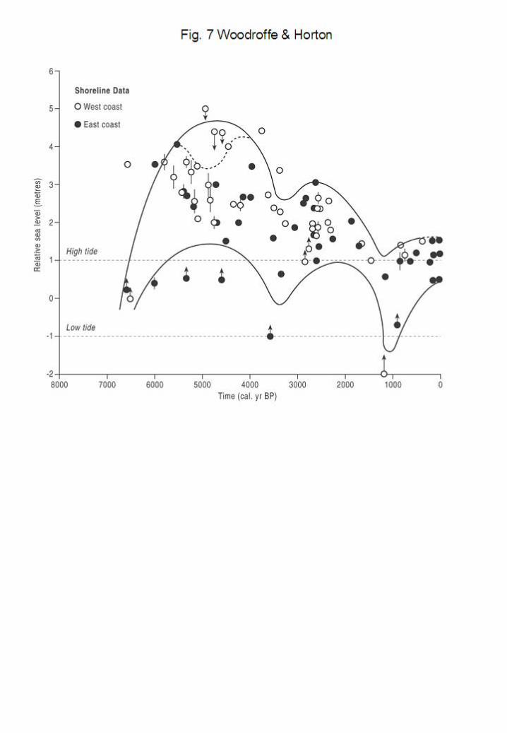
Holocene sea-level reconstructions in southeast Asia are limited and fragmentary. Tija (1996)

studied abrasion platforms, sea-level notches and oyster beds in Peninsula Malaysia and

produced over 130 radiocarbon-dated indicators. The sea-level curve, which proposes two

Holocene high stands at 5000 and 2800 14C yrs BP, does not take into account the broad

altitudinal range of the indicators, and the second high stand could easily be accounted for by error

terms in the general RSL drop after 5000 BP (Fig 7). Tija’s (1996) sea-level reconstruction for

Thailand, based mainly on peat, marine shells and mangrove wood, indicates potentially three

mid/late Holocene high stands at 6000, 4000 and 2700 14C yrs BP, which he attributes to sea level

lowering in a series of short periods of regression and transgression. Over 100 indicators were

taken from around the Peninsula Coast, therefore reflecting regional rather than local influences;

however it is hard to reconcile this model of sea-level history with the scattered evidence that is

presented. Scoffin and Le Tissier (1998) studied intertidal reef-flat corals (microatolls) for mid/late

Holocene high stands at Phuket, Southern Thailand. The evidence here suggests a single

Holocene high stand with a constant rate of RSL fall since 6000 cal yrs BP, and thus, contradicts

conclusions drawn by Tija (1996). However it should be noted that Scoffin and Le Tissier’s (1998)

research is from only one site with eleven dated samples.

Geyh and Kudrass (1979) conducted a study in the Strait of Malacca, Indonesia, which resulted in

33 directional (limiting) index points from 14C dated fossil mangrove deposits. These index points,

10

10

which are not given an indicative meaning, imply that Holocene sea level rose from below –12.8

m to ~1.2 m above present between 8000 and 6000 14C yrs BP, and between 5000 and 4000 14C

yrs BP rose to its highest recorded level in southeast Asia, at ~5.8 m above present (but this is a

limiting index point, uncorrected for indicative meaning). The data does not show whether the late

Holocene lowering of sea level was a steady or oscillatory process.

The Cocos Keeling Islands are a mid-oceanic atoll situated approximately 600km southwest of

Jakarta, Indonesia in the Indian Ocean. Their RSL history is recorded in massive coral and

microatolls. The microfossil record produces a detailed late Holocene RSL history showing a

single Holocene high stand after 3000 14C yrs BP of at least 0.5 m (Woodroffe and McLean, 1990).

4.4 Northern Asia

The areas grouped under this heading include Japan and southeast China, bordering the South

China Sea. Japan is forms part of a tectonically active island arc, which makes regional sea-level

comparisons difficult due to local and regional crustal flexure and warping. Nakada et al. (1991)

undertook RSL reconstructions from Osaka and Tokyo using previously published data and

showed a significant spatial dependence to the amplitude of the mid-Holocene high stand. Fixed

biological indicators (oyster beds) have been used at one site on the South China Sea coast to

infer the amplitude and timing of the mid-Holocene high stand; no greater than 2 m above modern

sea level at 5140 14C yrs BP (Yim and Huang, 2002). Further research using fixed biological

indicators is needed from other locations of the coastline in order to constrain the amplitude of the

mid-Holocene high stand and to better understand the effect of monsoon forcing on the RSL

record.

4.5 Australia Australia is a tectonically stable continent far from plate margins, situated at the centre of the

Australian-Indian plate, and as such should preserve a sea level record dominated by eustatic

processes. Fixed biological indicators such as tubeworms, oyster beds, barnacles and corals have

been used extensively along the east coast of Australia to infer Holocene sea-level movements

(e.g., Beaman et al., 1994, Baker and Haworth, 2000, Baker et al., 2001), and foraminifera have

been used to infer relative estuarine/lagoonal and oceanic influences through the Holocene in the

estuaries of South Australia (Cann et al. 1993, 2000a, 2000b, 2002). In the Northern Spencer Gulf

the highest Holocene sea levels occurred at 7000 cal years BP, followed by continuous RSL fall

through the late Holocene (Cann et al. 2000a). Studies from north New South Wales show a late

Holocene high stand at +1.7 m at 3810 cal yrs BP (Baker et al., 2001). However, evidence for the

11

11

mid-Holocene high stand in northeast Australia is much earlier, at 1.65 m above RSL between

5660-4040 14C yrs BP in Cleveland Bay, central Great Barrier Reef (Beaman et al., 1994).

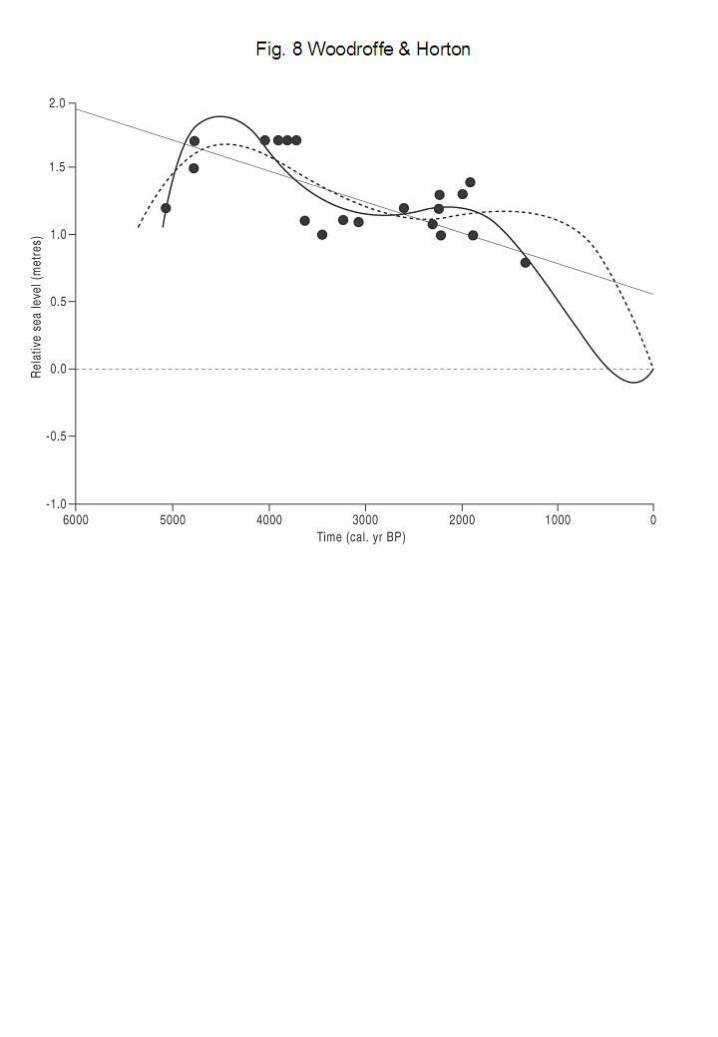
The eastern coast of Australia is affected by differential crustal flexure over late Holocene

timescales due to differences in the width of continental shelf and its impact on hydro-isostatic

adjustment (Flood and Frankel, 1989; Baker et al., 2001). This affects the timing of the mid-

Holocene high stand along the eastern Australian coast. Fig 8 illustrates that by fitting a

polynomial trendline through sea-level index points created from fixed biological indicators (Baker

et al. 2001) it is possible to draw the conclusion that two mid/late-Holocene high stands have

occurred in this region, if age and altitude errors in the reconstructions are not taken into account.

However there is little justification for choosing an episodic late Holocene sea level trend using

mathematical modelling which does not incorporate the range of potential values for each

age/altitude index point.

Larcombe et al. (1995) and Larcombe and Carter (1998) present evidence for an episodic early

Holocene marine transgression across the central Great Barrier Reef shelf. The most contentious

aspect is the evidence for a stillstand at –10 m at 8500 14C years BP, followed by a rapid fall in

RSL to –17 m at 8200 14C years BP, and then a rapid rise in RSL to –5 m by 7800 14C years BP.

The database used to infer this sea-level trend incorporates evidence from a wide range of studies

over a period of 25 years, by different researchers using different proxy indicators. The database

makes no attempt to reclassify indicators for the inferred sea-level position at the time the indicator

was lain down. Indicators from a wide geographical area (4 degrees of latitude) are included in a

single reconstruction, which would infer that differential crustal movement has not occurred over

this wide area during the Holocene. Evidence from other studies (Hopley 1975, Chappell et al.

1983) show that up to 3 m of differential movement has occurred along this coastline over the past

6000 years.

4.6 Pacific Ocean

The Holocene RSL history of the Pacific Ocean basin is of prime importance for furthering our

understanding of geoidal-eustasy, in particular Equatorial Ocean syphoning. A plethora of studies

have emerged in recent years from the oceanic atolls of the Pacific, most noticeably the Tahiti

coral record (Bard et al., 1996), and studies from Fiji, Kiribati, French Polynesia, Hawaii, Tonga,

Marshall Islands and others (e.g., Grossman et al., 1998, Nunn and Peltier 2001). The vast

majority of sea-level index points from the Pacific use massive coral species (Acropora and

Porites), coral microatolls or beachrock as indicators, which each have their own limitations. In

addition many, if not all, of the oceanic atolls of the Pacific are subject to tectonic movements over

12

12

Holocene and even longer timescales. Many studies assume stability over the Holocene,

whereas in fact slow, constant subsidence may be occurring. Mid/late Holocene sea-level records

from the Pacific have been interpreted as evidence for a migrating geoid, through evidence of

greater emergence in the central ocean basin interior during the mid/late Holocene, and most

significant and recent RSL fall in the central equatorial Pacific (Mitrovica and Peltier, 1991, Nunn

and Peltier, 2001). In addition sea-level observations indicate that oceanic atolls less than 10 km in

diameter are affected by hydro isostasy (Grossman et al., 1997).

5. Discussion

This review has illustrated the geographical variability of RSL reconstructions, and the variable

quality of reconstructions across the Indo-Pacific region. It has also shown that evidence for the

mid-Holocene high stand is variable in both magnitude and timing across the Indo-Pacific. In

several locations limited evidence points towards a second, smaller magnitude high stand in the

late Holocene (Table 1).

Field observations of mid-Holocene high stands provide essential constraints to geophysical

models because model predictions of these high stands depend upon three large-scale, high

amplitude, globally applicable mechanisms: ocean syphoning caused mainly by gravitational

effects due to the collapse of peripheral forebulges, continental levering associated with local

ocean loading, and on-going melting of global ice since the time of the high stand (magnitude and

source). The first two mechanisms occur throughout the deglaciation process, with the mid-

Holocene high stand marking a point in time when the eustatic signal reduces in magnitude so that

these solid earth processes become apparent in the RSL record. Syphoning and continental

levering are dependant on the viscosity structure and, thus, contribute to the sensitivity of different

models. Since syphoning produces a more geographically uniform sea-level fall than the

continental levering effect, the latter is likely to account for most of the site dependent variations of

predicted high stands. Differences between sea-level observations and predicted high stand

amplitudes are used to estimate the final mechanism; on-going melting of global ice since the time

of the high stand (Mitrovica and Peltier 1991, Peltier, 2002, Mitrovica and Milne 2002). If the

observations are measured precisely, they may provide constraints on where the meltwater came

from (northern or southern hemisphere), or at least the relative magnitudes.

Grossman et al. (1997) propose that a second, short-lived marine transgression in low and mid

latitudes in the late Holocene may be due to the migration of the geoid. The behaviour of the

migrating geoid might be as a series of oscillating waves flowing from its maximum position in the

central ocean basin interior (the central equitorial Pacific), rather than as migration as a single

peak. Low and mid latitudes might experience a slight, short-lived transgression and regression

13

13

due to the interplay between geoidal eustasy and hydro isostasy during the late Holocene period

when glacio-eustasy has ceased. In addition, Grossman et al. (1997) suggest that the geoidal

anomoly may decay in the Pacific towards the Asian continent, directing a second transgression to

this area only. This would fit with the evidence, which suggests that two Holocene high stands are

only witnessed in areas of the Indo Pacific far from the central equitorial Pacific. However this may

just be a coincidence considering the poor quality of the empirical data.

This review of far field locations has raised the issue that the fundamental criteria to produce an

accurate Holocene sea-level curve are hardly ever met. The accuracy or significance of each curve

depends upon the number of sea level index points, the correct interpretation of its relation to the

corresponding mean sea level, and the quality of age determinations. There are serious problems

associated with the correct interpretation of the elevational relationship of the sea-level indicators

to mean sea level. Different types of indicators have different degrees of precision, but this is often

not acknowledged. Coral microatolls in some settings have a much higher degree of precision than

other species such as Porites or Acropora, which have wide elevational ranges, but each study is

considered accurate to the same level. Elevation error ranges are rarely included on sea-level

curves. The indicative meaning and reference water level of each indicator is sometimes

accounted for, sometimes not. Different workers assign different indicative meanings to the same

indicator. It is common to use low tide level as a common datum rather than mean tide level, but

this is not often stated in reports, precluding regional correlation of different studies.

The second serious form of error regards age determinations, in particular the calibration of

radiocarbon dates, a necessary process because the assumption that the specific activity of the 14C in the atmospheric carbon dioxide has been constant is invalid. The 14C activity in the

atmosphere and other reservoirs, and thus in the initial activity of the samples dated, has varied

over time (e.g., Stuiver et al., 1998). A calibration dataset is necessary to convert conventional

radiocarbon ages (14C yr) into calibrated years (cal yr). However, many researchers do not

calibrate their radiocarbon dates, or fail to state in their publications whether they have or not. If

ages are calibrated, different researchers use different calibration programs, which use alternative

calibration terms and produce different results. Similar uncertainties are found with the application

of the Marine Reservoir Effect. Radiocarbon ages of samples formed in the ocean, such as shells,

fish, marine mammals etc., are generally several hundred years older than their terrestrial

counterparts. This apparent age difference is due to the large carbon reservoir of the oceans. A

correction is necessary in order to compare marine and terrestrial samples, but because of

complexities in ocean circulation the actual correction varies with location.

14

14

6. Conclusion

Thus, further sea-level analysis from far field locations must involve the application of the

consistent methodology to the reconstruction of sea-level history, which was first formalised during

International Geological Correlation Programme (IGCP) Project 61. This operated in the period

1979-1983, and has been a component of all subsequent IGCP Projects, especially Projects 200,

274, 367 and 437 (e.g., van de Plassche, 1986; Shennan and Horton, 2002), however this review

has shown serious failings in its application. A new generation of sea-level records from far field

locations will improve our understanding of the driving mechanisms behind Holocene sea-level

change and coastal evolution over a range of spatial and temporal scales. This sea-level data

could be meaningfully compared with the emerging high-precision palaeoenvironmental records

from the ice sheets (cores), the oceans (e.g., corals, high-resolution sediment cores) and other

terrestrial archives (e.g., peat bogs and loess sequences). Therefore, exploration of the

implications of sea-level records for an understanding of existing terrestrial and oceanic records of

Holocene environmental change, including the leads and lags associated with oceanic and

terrestrial records (e.g., Visser et al., 2003) could occur. This provides an improved scientific

background against which the role of humans as agents of coastal change can be appreciated.

7. Acknowledgements This research was carried out while in receipt of a Natural Environment Research Council award

(NER/S/C/2002/10581). Special acknowledgements are given to Operation Wallacea, and to S.

Smithers and D. Smith for their valuable comments on the original version of this paper. The

authors thank the cartography department at the Department of Geography, University of Durham

for producing the figures, and to all members of the Environmental Research Centre, University of

Durham for their help and advice. This paper is a contribution to IGCP project 437.

References

Agassiz, L., 1840. Etudes sur les glaciers, privately published, Neuchtel.

Alley, R.B., Clark, P.U., 1999. The deglaciation of the northern hemisphere: a

global perspective. Annual Review of Earth and Planetary Science 27, 149-

182.

Baker, R.G.V., Haworth, R.J., 2000. Smooth or oscillating late Holocene sea-

level curve? Evidence from cross-regional statistical regressions of fixed

biological indicators. Marine Geology 163, 353-365.

Baker, R.G.V., Haworth, R.J., Flood, P.G., 2001. Inter-tidal fixed indicators of

former Holocene sea-levels in Australia: a summary of sites and a review of

methods and models. Quaternary International 83-85, 257-273.

Banjeree, P.K., 2000. Holocene and Late Pleistocene relative sea level

fluctuations along the east coast of India. Marine Geology 167, 243-260.

Bard, E., Hamelin, B., Arnold, M., Montaggioni, L., Cabioch, G., Faure, G.,

Rougerie, F.,1996. Deglacial sea-level record from Tahiti corals and the timing

of global meltwater discharge. Nature 382, 241-244.

Beaman, R., Larcombe, P., Carter, R.M., 1994. New evidence for the

Holocene sea-level high from the inner shelf, Central Great Barrier Reef,

Australia. Journal of Sedimentary Research A64 (4), 881-885.

Blanchon, P., Shaw, J., 1995. Reef drowning during the last deglaciation:

Evidence for catastrophic sea-level rise and ice-sheet collapse. Geology, 23

(1), 4-8.

Broecker, W.S., Denton, G.H., 1989. The role of ocean-atmosphere

reorganizations in glacial cycles. Geochimica et Cosmochimica Acta 53,

2465-2501.

Camoin, G.F., Colonna, M., Montaggioni, L.F., Casanova, J., Faure, G.,

Thomassin, B.A., 1997. Holocene sea level changes and reef development in

the southwestern Indian Ocean. Coral Reefs 16, 247-259.

Cann, J. H., Belperio, A. P., Gostin, V. A., Rice, R. L. 1993. Contemporary

benthic foraminifera in Gulf St. Vincent, South Australia, and a refined Late

Pleistocene sea-level history. Australian Journal of Earth Sciences 40, 197-

211.

Cann, J. H., Belperio, A. P., Murray-Wallace, C. V. 2000a. Late Quaternary

palaeosealevels and palaeoenvironments inferred from foraminifera, northern

Spencer Gulf, South Australia. Journal of Foraminiferal Research, 30, 29-53.

Cann, J. H., Bourman, R. P., Barnett, E. J. 2000b. Holocene foraminifera as

indicators of relative estuarine-lagoonal and oceanic influences in estuarine

sediments of the River Murray, South Australia. Quaternary Research, 53,

378-391.

Cann, J. H., Harvey, N., Barnett, E. J., Belperio, A. P., Bourman, R. P. 2002.

Foraminiferal biofacies ecosuccession and Holocene sealevels, Port Pirie,

South Australia. Marine Micropalaeontology, 44, 31-55.

Chappell, J., Chivas, A., Wallensky, E., Polach, H. A., Aharon, P., 1983.

Holocene palaeo-environmental changes, central to north Great Barrier Reef

inner zone. BMR Journal of Australian Geology and Geophysics 8, 223-235.

Chappell, J., Polach, H., 1991. Postglacial sea-level rise from a coral record at

Huon Peninsula, Papua New Guinea. Nature 349, 147-149.

Clark, J.A., Farrell, W.E, Peltier, W.R., 1978. Global changes in post glacial

sea level: a numerical calculation. Quaternary Research 9, 265-287.

Clark, P.U., Alley, R.B., Keigwin, L.D., Licciardi, J.M., Johnsen, S.J., Wang,

H.X., 1996. Origin of the first global meltwater pulse following the last glacial

maximum. Paleoceanography 11, 563-577.

Clark, P.U., Mitrovica, J.X., Milne, G.A., Tamisiea, M.E., 2002. Sea-level

fingerprinting as a direct test for the source of global meltwater pulse IA.

Science 295, 2438-2441.

Colonna, M., Casanova, J., Dullo, W.C., Camoin, G., 1996. Sea-level changes

and d180 record for the past 34,000 yr from Mayotte Reef, Indian Ocean.

Quaternary Research 46, 335-339.

Compton, J.S., 2001. Holocene sea-level fluctuations inferred from the

evolution of depositional environments of the southern Langebaan Lagoon

salt marsh, South Africa. The Holocene 11(4), 395-405.

Daly, R.A., 1934. The Changing world of the ice age. Yale University Press,

New Haven.

Dickinson, W.R., 2001. Paleoshoreline record of relative Holocene sea levels

on Pacific islands. Earth Science Reviews 55, 191-234.

Done, T. J., 1982. Patterns in the distribution of coral communities across the

central Great Barrier Reef shelf. Coral Reefs, 1, 95-108.

Fairbanks, R.G., 1989. A 17,000-year glacio-eustatic sea level record:

influence of glacial melting rates on the Younger Dryas event and deep-ocean

circulation. Nature 342, 639-642.

Fleming, K., Yokoyama, Y., Lambeck, K., Chappell, J., Johnston, P., Zwartz,

D., 1998. Refining the eustatic sea-level curve since the Last Glacial

Maximum using far- and intermediate-field sites. Earth and Planetary Science

Letters, 163(1-4), 327-342.

Flood, P.G., Frankel, E. 1989. Late Holocene higher sea level indicators from

eastern Australia. Marine Geology 90, 193-195.

Geyh, M. A., Kudrass, H-R. 1979. Sea-level changes during the late

Pleistocene and Holocene in the Strait of Malacca. Nature 278, 441-443.

Grossman, E.E., Fletcher III, C.H., Richmond, B.M., 1998. The Holocene sea-

level high stand in the equatorial Pacific: analysis of the insular paleosea-level

database. Coral Reefs 17, 309-327.

Hanebuth, T., Stattegger, K., Grootes, P.M., 2000. Rapid flooding of the

Sunda Shelf: a Late-Glacial sea-level record. Science 288, 1033-1035.

Hopley, D., 1975. Contrasting evidence for Holocene sea levels with special

reference to the Bowen-Whitsunday area of Queensland. In Douglas, I.,

Hobbs, J. E., and Pigram, J. J. (Eds) Geographical Essays in Honour of

Gilbert J. Butland, Department of Geography, University of New England,

Armidale, 51-84.

Horton, B.P., Edwards, R.J., Lloyd, J.M., 2000. Implications of a microfossil

transfer function in Holocene sea level studies. In: Shennan, I and Andrews,

J. (Eds.) Holocene land-ocean interaction and environmental change around

the North Sea. Geological Society, London. Special Publications 166, 275-

298.

Houghton, J.T., Ding, Y., Griggs, D.J., Noguer, M., van der Linden, P.J.,

Xiaosu, D. 2001. Contribution of Working Group I to the third Assessment

Report of the Intergovernmental Panel on Climate Change (IPCC), Cambridge

University Press.

Islam, M.S., Tooley, M.J. 1999. Coastal and sea-level changes during the

Holocene in Bangladesh. Quaternary International 55, 61-75.

Katupotha, J., Fujiwara, K., 1988. Holocene sea level change on the

Southwest and South coasts of Sri Lanka. Palaeogeography,

Palaeoclimatology, Palaeoecology, 68, 189-203.

Lambeck, K., Chappell, J., 2001. Sea level change through the last glacial

cycle. Science 292, 679-686.

Lambeck , K., Esat, T.M., Potter, E-K., 2002. Links between climate and sea

levels for the past three million years. Nature 419, 199-206.

Lambeck, K., Purcell, A., Johnston, P., Nakada, M., Yokoyama, Y., 2003.

Water-load definition in the glacio-hydro-isostatic sea-level equation.

Quaternary Science Reviews 22 (2-4), 309-318.

Larcombe, P., Carter, R.M., Dye, J., Gagan, M. K., Johnson, D.P. 1995. New

evidence for episodic post-glacial sea level rise, central Great Barrier Reef,

Australia. Marine Geology, 127, 1-44.

Larcombe, P., Carter, R.M. 1998. Sequence architecture during the Holocene

transgression : an example from the Great Barrier Reef shelf, Australia.

Sedimentary Geology, 117, 97-121.

Li, L., Gallagher, S., Finlayson, B. 2000. Foraminiferal response to Holocene

environmental changes of a tidal estuary in Victoria, southeastern Australia.

Marine Micropalaeontology, 38, 229-246.

Lighty, R. G., Macintyre, I. G., Stuckenrath, R. 1982. Acropora palmata reef

framework: a reliable indicator of sea level in the Western Atlantic for the past

10,000 years. Coral Reefs, 1, 125-130.

Long, A.J., 2000. Late Holocene sea-level change and climate. Progress in

Physical Geography 24, 415-423.

McManus, J.F., Oppo, D.W. Cullen, J.L., 1999. A 0.5-million-year record of

millennial-scale climate variability in the North Atlantic. Science 283, 971-975.

Mitrovica, J.X., 2003. Recent controversies in predicting post-glacial sea-level

change. Quaternary Science Reviews 22 (2-4), 127-133.

Mitrovica, J.X., Milne, G.A., 2002. On post-glacial sea level 1: General theory.

Geophysical Journal International 133, 1-19.

Mitrovica, J.X., Peltier, W.R., 1991. On postglacial geoid subsidence over the

equitorial oceans. Journal of Geophysical Research 96 (B12), 20053-20071.

Mörner, N.-A., 1976. Eustasy and geoid changes. Journal of Geology 84, 123-

151.

Mörner, N.-A., 1996. Rapid changes in coastal sea level. Journal of Coastal

Research 12, 797-800.

Nakada, M., Yonekura, N., Lambeck, K., 1991. Late Pleistocene and

Holocene sea-level changes in Japan: implications for tectonic histories and

mantle rheology. Palaeogeography, Palaeoclimatology, Palaeoecology 85,

107-122.

Nunn, P.D., 1998. Sea-Level changes over the past 1000 years in the Pacific.

Journal of Coastal Research 14, 23-30.

Nunn, P.D., Peltier, W.R., 2001. Far-field test of the ICE-4G model of global

isostatic response to deglaciation using empirical and theoretical Holocene

sea-level reconstructions for the Fiji Islands, Southwestern Pacific.

Quaternary Research 55, 203-214.

Peltier, W.R., 1998. Postglacial variations in the level of the sea: implications

for climate dynamics and solid-Earth geophysics. Reviews of Geophysics 36 ,

603–689.

Peltier, W.R., 2002. On eustatic sea level history: Last Glacial Maximum to

Holocene. Quaternary Science Reviews 21, 377-396.

van de Plassche, O., (Ed.) 1986. Sea-level research: a manual for the

collection and evaluation of data. Geobooks, Norwich.

Pirazzoli, P.A., 1991. World atlas of Holocene sea-level changes. Elsevier,

Amsterdam, Oceanography Series, vol. 58.

Pirazzoli, P.A., 1996. Sea-level changes: the last 20 000 years. Wiley,

Chichester.

Ramsay, P.J., 1995. 9000 years of sea-level change along the southern

African coastline. Quaternary International 31, 71-75.

Ramsay, P.J., Cooper, J.A.G., 2002. Late Quaternary sea-level change in

South Africa. Quaternary Research 57, 82-90.

Sawai, Y., Nasu, H., Yasuda, Y., 2002. Fluctuations in relative sea-level

during the past 3000 yr in the Onnetoh estuary, Hokkaido, northern Japan.

Journal of Quaternary Science, 17, 607-622.

Scoffin, T.P., Le Tissier, M.D.A., 1998. Late Holocene sea level and reef-flat

progradation, Phuket, South Thailand. Coral Reefs 17, 273-276.

Shennan, I., Horton, B.P., 2002. Holocene land and sea-level changes in

Great Britain. Journal of Quaternary Science 17, 511-526.

Shennan, I., Peltier, W.R., Drummond, R. and Horton, B.P. 2002. Global to

local scale parameters determining relative sea-level changes and the post-

glacial isostatic adjustment of Great Britain. Quaternary Science Reviews, 21,

397-408.

Smithers, S.G., Woodroffe, C.D., 2000. Microatolls as sea-level indicators on

a mid-ocean atoll. Marine Geology 168, 61-78.

Stuiver, M., Reimer, P. J. 1993. Extended 14C database and revised CALIB

radiocarbon calibration program. Radiocarbon, 35, 215-230.

Stuiver, M., Reimer, P.J., Bard, E., Beck, J.W., Burr, G.S., Hughen, K.S.,

Kromer, B., McCormac, F.G., van der Plicht, J., Spurk, M., 1998. INTCAL98

Radiocarbon Age Calibration, 24,000-0 cal BP. Radiocarbon 40, 1041-1083.

Stuiver, M., Reimer, P.J., Braziunas, T.F. ,1998. High precision radiocarbon

age calibration for terrestrial and marine samples Radiocarbon 40, 1127-

1151.

Suess, E., 1888. Das Anlitz der Erde, II: Die Meere der Erde. Wien.

Tija, H.D., 1996. Sea-level changes in the tectonically stable Malay-Thai

Peninsula. Quaternary International 31, 95-101.

Visser, K., Thunell, R., Stott, L., 2003. Magnitude and timing of temperature

change in the Indo-Pacific warm pool during deglaciation. Nature 421, 152 -

155

Woodroffe, C.D., McLean, R., 1990. Microatolls and recent sea-level change

on coral atolls. Nature 344, 531-534.

Yim, W.W.-S., Huang, G., 2002. Middle Holocene higher sea-level indicators

from the South China coast. Marine Geology 182(3-4), 225-230.

Yokoyama, Y., Lambeck, K., De Deckker, P., Johnston, P., Fifield, L.K., 2000.

Timing of the Last Glacial Maximum from observed sea-level minima. Nature

406, 713-716.

Zong, Y., Shennan, I., Combellick, R. A., Hamilton, S. L., Rutherford, M. M.,

2003. Microfossil evidence for land movements associated with the AD 1964

Alaska earthquake. The Holocene, 13, 7-20.

LIST OF FIGURES

FIGURE 1. The relative sea-level curve for the last glacial cycle for Huon Peninsula

(Lambeck and Chappell, 2001) supplemented with observations from Bonaparte Gulf,

Australia (Yokoyama et al., 2000). Error bars define the upper and lower limits (modified

from Lambeck et al., 2002).

FIGURE 2. Sea-level zones and typical relative sea-level curves deduced for each zone

by Clark et al. (1978) under the assumption that no eustatic change has occurred since 5

ka BP.

FIGURE 3. Schematic diagram of the Indicative Meaning illustrating the how the Indicative

Range (IR) and Reference Water Level (RWL) are derived from Mean Tide Level (MTL)

(not drawn to scale).

FIGURE 4. Sea-level history reconstructed for long drill cores from Tahiti (triangles),

Barbados (squares) and Papua New Guinea (dots). All radiocarbon dates have been

corrected to calendar years and all data points have been appropriately corrected for

uplift/subsidence.

FIGURE 5. Location of sea-level reconstructions in the Indo-Pacific region. Numbers refer

to locations in Table 1.

FIGURE 6. Holocene sea-level fluctuations inferred from sea-level index points from the

southern Langebaan Lagoon salt marsh, South Africa. Horizontal error bars refer to

analytical uncertainty in radiocarbon age calibration (2σ range), and vertical error bars

refer to uncertainty in sea level predictions derived from organic matter and shell material

indicators (modified from Compton, 2001).

FIGURE 7. Holocene sea-level envelope for Peninsula Malaysia (modified from Tija 1996).

Data points with arrows indicate directional (limiting) index points. Some index points have

vertical error bars, where the vertical range of the sea-level indicator is understood. No

age errors are considered, radiocarbon ages are plotted. The boundaries of the envelope

are drawn midway between the extreme data points and the neighbouring points within the

envelope (Tija 1996).

FIGURE 8. A summary of linear and oscillating regression models from sea-level index

points created using fixed biological indicators from SE Australia for the past 5000 years.

Dotted line – 4th order polynomial (r2 = 0.69), smooth line – 5th order polynomial (r2 = 0.78)

(after Baker et al. 2001).

LIST OF TABLES

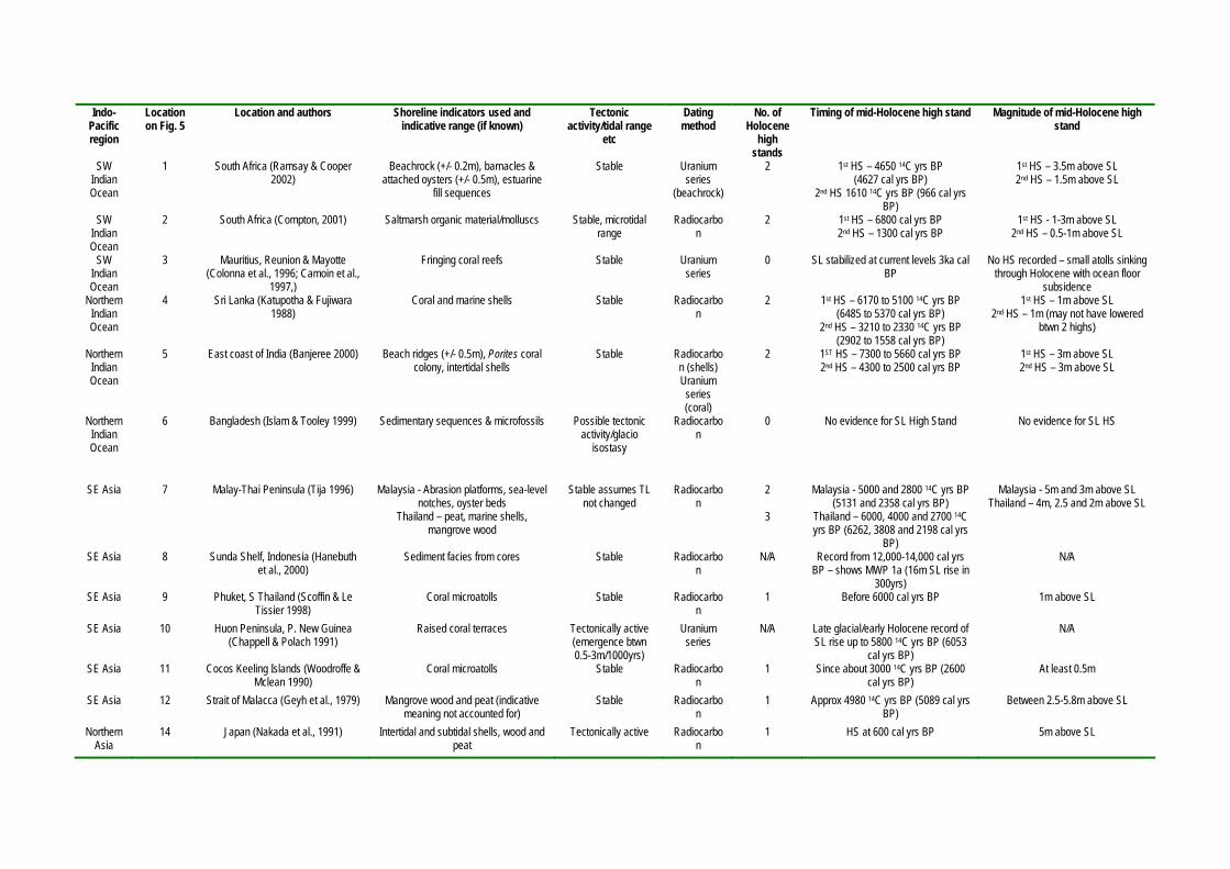
TABLE 1. Details of sea-level reconstructions from the Indo-Pacific region (HS = high

stand). Radiocarbon ages calibrated to 2σ using the probability method in the program

CALIB rev. 4.3, (Stuiver and Reimer 1993), including corrections for the marine reservoir

effect using the calibration data of Stuiver et al. (1998).

Indo-

Pacific region

Location on Fig. 5

Location and authors Shoreline indicators used and indicative range (if known)

Tectonic activity/tidal range

etc

Dating method

No. of Holocene

high stands

Timing of mid-Holocene high stand Magnitude of mid-Holocene high stand

SW Indian Ocean

1 South Africa (Ramsay & Cooper 2002)

Beachrock (+/- 0.2m), barnacles & attached oysters (+/- 0.5m), estuarine

fill sequences

Stable

Uraniumseries

(beachrock)

2 1st HS – 4650 14C yrs BP (4627 cal yrs BP)

2nd HS 1610 14C yrs BP (966 cal yrs BP)

1st HS – 3.5m above SL 2nd HS – 1.5m above SL

SW Indian Ocean

2 South Africa (Compton, 2001) Saltmarsh organic material/molluscs

Stable, microtidal range

Radiocarbon

2 1st HS – 6800 cal yrs BP 2nd HS – 1300 cal yrs BP

1st HS - 1-3m above SL 2nd HS – 0.5-1m above SL

SW Indian Ocean

3 Mauritius, Reunion & Mayotte (Colonna et al., 1996; Camoin et al.,

1997,)

Fringing coral reefs Stable Uranium series

0 SL stabilized at current levels 3ka cal BP

No HS recorded – small atolls sinking through Holocene with ocean floor

subsidence Northern

Indian Ocean

4 Sri Lanka (Katupotha & Fujiwara 1988)

Coral and marine shells Stable Radiocarbon

2 1st HS – 6170 to 5100 14C yrs BP (6485 to 5370 cal yrs BP)

2nd HS – 3210 to 2330 14C yrs BP (2902 to 1558 cal yrs BP)

1st HS – 1m above SL 2nd HS – 1m (may not have lowered

btwn 2 highs)

Northern Indian Ocean

5 East coast of India (Banjeree 2000) Beach ridges (+/- 0.5m), Porites coral colony, intertidal shells

Stable Radiocarbon (shells) Uranium

series (coral)

2 1ST HS – 7300 to 5660 cal yrs BP 2nd HS – 4300 to 2500 cal yrs BP

1st HS – 3m above SL 2nd HS – 3m above SL

Northern Indian Ocean

6 Bangladesh (Islam & Tooley 1999) Sedimentary sequences & microfossils Possible tectonic activity/glacio

isostasy

Radiocarbon

0 No evidence for SL High Stand No evidence for SL HS

SE Asia 7 Malay-Thai Peninsula (Tija 1996) Malaysia - Abrasion platforms, sea-level notches, oyster beds

Thailand – peat, marine shells, mangrove wood

Stable assumes TL not changed

Radiocarbon

2

3

Malaysia - 5000 and 2800 14C yrs BP (5131 and 2358 cal yrs BP)

Thailand – 6000, 4000 and 2700 14C yrs BP (6262, 3808 and 2198 cal yrs

BP)

Malaysia - 5m and 3m above SL Thailand – 4m, 2.5 and 2m above SL

SE Asia 8 Sunda Shelf, Indonesia (Hanebuth et al., 2000)

Sediment facies from cores Stable Radiocarbon

N/A Record from 12,000-14,000 cal yrs BP – shows MWP 1a (16m SL rise in

300yrs)

N/A

SE Asia 9 Phuket, S Thailand (Scoffin & Le Tissier 1998)

Coral microatolls Stable Radiocarbon

1 Before 6000 cal yrs BP 1m above SL

SE Asia 10 Huon Peninsula, P. New Guinea (Chappell & Polach 1991)

Raised coral terraces Tectonically active (emergence btwn 0.5-3m/1000yrs)

Uranium series

N/A Late glacial/early Holocene record of SL rise up to 5800 14C yrs BP (6053

cal yrs BP)

N/A

SE Asia 11 Cocos Keeling Islands (Woodroffe & Mclean 1990)

Coral microatolls Stable Radiocarbon

1 Since about 3000 14C yrs BP (2600 cal yrs BP)

At least 0.5m

SE Asia 12 Strait of Malacca (Geyh et al., 1979) Mangrove wood and peat (indicative meaning not accounted for)

Stable Radiocarbon

1 Approx 4980 14C yrs BP (5089 cal yrs BP)

Between 2.5-5.8m above SL

Northern Asia

14 Japan (Nakada et al., 1991) Intertidal and subtidal shells, wood and peat

Tectonically active Radiocarbon

1 HS at 600 cal yrs BP 5m above SL

Northern Asia

15 Japan (Sawai et al. 2002) Sedimentary sequences and microfossils

Tectonically active Radiocarbon

N/A 3 falls in RSL since 3000 cal yrs BP N/A

Northern Asia

16 Southeast China (Yim & Huang, 2002)

Fixed biological indicators (oyster beds) Local monsoon activity

Radiocarbon

1

5140 14C yrs BP (5371 cal yrs BP) No more than 2m above SL

Australia 17 Central Great Barrier Reef, Australia (Beaman et al., 1994; Larcombe et

al., 1995; Larcombe and Carter, 1998)

Oyster beds Stable, some differential flexing of shelf over past 6000

yrs

Radiocarbon

1 Between 5660 and 4040 14C yrs BP (6000 and 4053 cal yrs BP)

1.65m above SL

Australia 18 Eastern Australia (Flood & Frankel 1989)

Intertidal tube worms Stable Radiocarbon

1 Some time before and after 3420 14C yrs BP (3274 cal yrs BP)

At least 1m above SL

Australia 19 Bonaparte Gulf, NE Australia (Yokoyama et al., 2000)

Sedimentary facies and their contained microfossils

Stable Radiocarbon

N/A LGM and early late glacial record N/A

Australia 20 New South Wales (Baker et al., 2001)

Fixed biological indicators (tubeworms, barnacles, oysters)

Stable Radiocarbon

1 Around 3900 cal yrs BP At least 1m above SL

Pacific 21 Fiji (Nunn & Peltier 2001) Coral (Porites) microatolls and intertidal shells from raised beaches

Hotspot activity over Holocene timescales

(subsidence)

Radiocarbon

1 or 2 1st HS – 5650 to 3200 14C yrs BP (6021 to 2939 cal yrs BP)

2nd HS – 6100 to 4550 and 3590 to 2800 14C yrs BP (6477 to 4678 and

3422 to 2485 cal yrs BP)

1st HS – 1.35 to 1.5m above SL 2nd HS – (i) 0.75-1.85m, (ii) 0.90-

2.46m above SL

Pacific 22 Taihiti (Bard et al., 1996) Coral (Acropora) Slight subsidence(~0.2mm/yr)

Uranium series

N/A Record from 14,000-5000 cal yrs BP, shows MWP 1A

N/A

Pacific 23 W Central Equitorial Pacific (Grossman et al., 1998)

Coral, microatolls, beachrock, molluscs, peat

Hotspot activity over Holocene

Radiocarbon

1 4ka 14C yrs BP (3942 cal yrs BP) 1-2m above SL