Dornbusch Model
Some weaknesses of preceding models:
Monetary Model: exchange rates are far more volatile than monetaryvariables (and prices) than implied by dataM-F Model: with fixed prices policy conclusions are valid only in shortrun,
Dornbusch (1976) hybrid:
Short run properties of Keynesian modelsLong run properties of Monetary Model
Ozan Hatipoglu (Department of Economics) Open Economy Macroeconomics Spring 2017 159 / 196
Dornbusch Model
Some weaknesses of preceding models:
Monetary Model: exchange rates are far more volatile than monetaryvariables (and prices) than implied by data
M-F Model: with fixed prices policy conclusions are valid only in shortrun,
Dornbusch (1976) hybrid:
Short run properties of Keynesian modelsLong run properties of Monetary Model
Ozan Hatipoglu (Department of Economics) Open Economy Macroeconomics Spring 2017 159 / 196
Dornbusch Model
Some weaknesses of preceding models:
Monetary Model: exchange rates are far more volatile than monetaryvariables (and prices) than implied by dataM-F Model: with fixed prices policy conclusions are valid only in shortrun,
Dornbusch (1976) hybrid:
Short run properties of Keynesian modelsLong run properties of Monetary Model
Ozan Hatipoglu (Department of Economics) Open Economy Macroeconomics Spring 2017 159 / 196
Dornbusch Model
Some weaknesses of preceding models:
Monetary Model: exchange rates are far more volatile than monetaryvariables (and prices) than implied by dataM-F Model: with fixed prices policy conclusions are valid only in shortrun,
Dornbusch (1976) hybrid:
Short run properties of Keynesian models
Long run properties of Monetary Model
Ozan Hatipoglu (Department of Economics) Open Economy Macroeconomics Spring 2017 159 / 196
Dornbusch Model
Some weaknesses of preceding models:
Monetary Model: exchange rates are far more volatile than monetaryvariables (and prices) than implied by dataM-F Model: with fixed prices policy conclusions are valid only in shortrun,
Dornbusch (1976) hybrid:
Short run properties of Keynesian modelsLong run properties of Monetary Model
Ozan Hatipoglu (Department of Economics) Open Economy Macroeconomics Spring 2017 159 / 196
Dornbusch Model
Empirical observation: financial markets adjust to shocks far morerapidly than goods markets. Exchange rates fluctuations more violentthan could be explained by movements in relative real money suppliesor real incomes that are rather sluggish.
Consequence for modeling: in the short run, financial markets have tooveradjust in order to compensate for sluggish goods markets. Forexample exchange rates overshoot.
Why? With prices fixed in the short run, and any change in thenominal money is a change in real money supply and requires theinterest rate to adjust to clear the money market, because output isalso fixed in the very SR. (Liquidity Effect).
Ozan Hatipoglu (Department of Economics) Open Economy Macroeconomics Spring 2017 160 / 196
Dornbusch Model
However, deviations from the world interest rate is only temporary(UIRP holds). as product prices adjust, real money stock reversesitself, in fact the whole process goes into reverse.
In the long run, prices adjust fully, returning all real variables to theirpre-shock levels, but leaving the nominal exchange rate at the newequilibrium level predicted by the simple Monetary Model
Overshooting can also refer to the response to a real disturbance suchas an ’oil shock’.
Exchange rate expectations are not static. If exchange rates below itslong run equilibrium value it will up towards it. It will converge fasterthe further away (to LR equilibrium value) it is at any moment.Dornbusch model further offers a specific way of determiningexchange rate expectations as explained below.
Ozan Hatipoglu (Department of Economics) Open Economy Macroeconomics Spring 2017 161 / 196
Dornbusch Model Assumptions
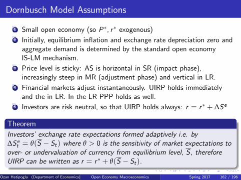
1 Small open economy (so P∗, r ∗ exogenous)
2 Initially, equilibrium inflation and exchange rate depreciation zero andaggregate demand is determined by the standard open economyIS-LM mechanism.
3 Price level is sticky: AS is horizontal in SR (impact phase),increasingly steep in MR (adjustment phase) and vertical in LR.
4 Financial markets adjust instantaneously. UIRP holds immediatelyand the in LR. In the LR PPP holds as well.
5 Investors are risk neutral, so that UIRP holds always: r = r ∗ + ∆Se
Theorem
Investors’ exchange rate expectations formed adaptively i.e. by∆Se
t = θ(S − St) where θ > 0 is the sensitivity of market expectations toover- or undervaluation of currency from equilibrium level, S , thereforeUIRP can be written as r = r ∗ + θ(S − St).
Ozan Hatipoglu (Department of Economics) Open Economy Macroeconomics Spring 2017 162 / 196
Dornbusch Model Assumptions
1 Small open economy (so P∗, r ∗ exogenous)
2 Initially, equilibrium inflation and exchange rate depreciation zero andaggregate demand is determined by the standard open economyIS-LM mechanism.
3 Price level is sticky: AS is horizontal in SR (impact phase),increasingly steep in MR (adjustment phase) and vertical in LR.
4 Financial markets adjust instantaneously. UIRP holds immediatelyand the in LR. In the LR PPP holds as well.
5 Investors are risk neutral, so that UIRP holds always: r = r ∗ + ∆Se
Theorem
Investors’ exchange rate expectations formed adaptively i.e. by∆Se
t = θ(S − St) where θ > 0 is the sensitivity of market expectations toover- or undervaluation of currency from equilibrium level, S , thereforeUIRP can be written as r = r ∗ + θ(S − St).
Ozan Hatipoglu (Department of Economics) Open Economy Macroeconomics Spring 2017 162 / 196
Dornbusch Model: Expectations
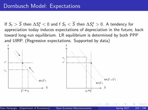
If St > S then ∆Set < 0 and f St < S then ∆Se
t > 0. A tendency forappreciation today induces expectations of depreciation in the future, backtoward long-run equilibrium. LR equilibrium is determined by both PPPand UIRP. (Regressive expectations. Supported by data)
r*
0S
S
r
1S
r1
1S
S
r
1S
r1
0( )RP S
1 0( )RP S S>1( )RP S
r*
Ozan Hatipoglu (Department of Economics) Open Economy Macroeconomics Spring 2017 163 / 196
Dornbusch Model
r
S
r0 A
r
y0y
IS(G0,Q0)
P
S0
SA
P
y0y
y0P0
0( )RP S
0S
0 0( / )LM M P
*0 0 /Q SP P=
AS(LR)
AS(SR)
*0 0 0 0( , , )AD G M S P
Ozan Hatipoglu (Department of Economics) Open Economy Macroeconomics Spring 2017 164 / 196
Dornbusch Model: Monetary Expansion
!"
#"
"!$""%
!"
&$"&"
'#()$*"+$,"
-"
#"
.
-"
&$"&"
/0$"1234"
&$"-$"
0( )RP S
0S
*0 0 /Q SP P=
%#(56,"
%#(#6,"
"!7"""!7""
"!$""
1( )RP S
1S
0S
1S
-7"
."
8
%
8
'#()$*"+7,"
&7"
&7"
1S
1S
%#(#6,"
%9()$":$*"#7"-$;,"
%9()$":$*"#<=!
7"-$;,"
%9()$":$*"#<=!
$-$;,"
5:"(:$>-$,"
5:"(:7>-$,"
Ozan Hatipoglu (Department of Economics) Open Economy Macroeconomics Spring 2017 165 / 196
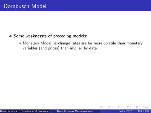
Dornbusch Model: Monetary Expansion Long Run Effects
Long Run effects:
AS is vertical which means that in LR there is no change in eq. realincome y0 and P ↑ such that to acommodate the increase in moneysupply such that we have eq in both money ( an increase in moneydemand to match the increase in money supply) and goods markets(an increase in interest rates r starting from the initial lower rates thatresult from an increase in Ms).In LR PPP holds, i.e. Q = SP∗/P, since prices are higher therefore S↑ in the long run. RP curve shifts rightWe have current account equilibrium due to instantaneous adjustmentof CPA and PPP.IS and LM are in original positions
Ozan Hatipoglu (Department of Economics) Open Economy Macroeconomics Spring 2017 166 / 196
Dornbusch Model: Monetary Expansion Long Run Effects
Long Run effects:
AS is vertical which means that in LR there is no change in eq. realincome y0 and P ↑ such that to acommodate the increase in moneysupply such that we have eq in both money ( an increase in moneydemand to match the increase in money supply) and goods markets(an increase in interest rates r starting from the initial lower rates thatresult from an increase in Ms).
In LR PPP holds, i.e. Q = SP∗/P, since prices are higher therefore S↑ in the long run. RP curve shifts rightWe have current account equilibrium due to instantaneous adjustmentof CPA and PPP.IS and LM are in original positions
Ozan Hatipoglu (Department of Economics) Open Economy Macroeconomics Spring 2017 166 / 196
Dornbusch Model: Monetary Expansion Long Run Effects
Long Run effects:
AS is vertical which means that in LR there is no change in eq. realincome y0 and P ↑ such that to acommodate the increase in moneysupply such that we have eq in both money ( an increase in moneydemand to match the increase in money supply) and goods markets(an increase in interest rates r starting from the initial lower rates thatresult from an increase in Ms).In LR PPP holds, i.e. Q = SP∗/P, since prices are higher therefore S↑ in the long run. RP curve shifts right
We have current account equilibrium due to instantaneous adjustmentof CPA and PPP.IS and LM are in original positions
Ozan Hatipoglu (Department of Economics) Open Economy Macroeconomics Spring 2017 166 / 196
Dornbusch Model: Monetary Expansion Long Run Effects
Long Run effects:
AS is vertical which means that in LR there is no change in eq. realincome y0 and P ↑ such that to acommodate the increase in moneysupply such that we have eq in both money ( an increase in moneydemand to match the increase in money supply) and goods markets(an increase in interest rates r starting from the initial lower rates thatresult from an increase in Ms).In LR PPP holds, i.e. Q = SP∗/P, since prices are higher therefore S↑ in the long run. RP curve shifts rightWe have current account equilibrium due to instantaneous adjustmentof CPA and PPP.
IS and LM are in original positions
Ozan Hatipoglu (Department of Economics) Open Economy Macroeconomics Spring 2017 166 / 196
Dornbusch Model: Monetary Expansion Long Run Effects
Long Run effects:
AS is vertical which means that in LR there is no change in eq. realincome y0 and P ↑ such that to acommodate the increase in moneysupply such that we have eq in both money ( an increase in moneydemand to match the increase in money supply) and goods markets(an increase in interest rates r starting from the initial lower rates thatresult from an increase in Ms).In LR PPP holds, i.e. Q = SP∗/P, since prices are higher therefore S↑ in the long run. RP curve shifts rightWe have current account equilibrium due to instantaneous adjustmentof CPA and PPP.IS and LM are in original positions
Ozan Hatipoglu (Department of Economics) Open Economy Macroeconomics Spring 2017 166 / 196
Dornbusch Model: Monetary Expansion Impact Effects
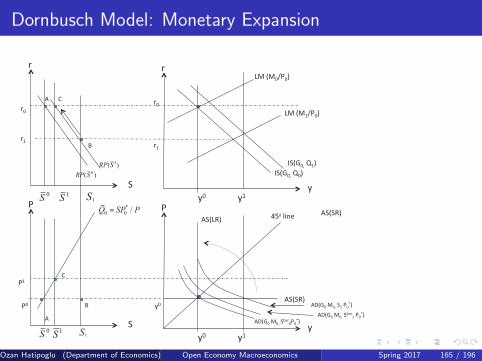
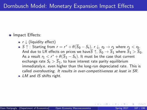
Impact Effects:
r ↓ (liquidity effect)S ↑ : Starting from r = r∗ + θ(S0 − St), r ↓, r0 → r1 where r1 < r0.And due to LR effects on prices we haveS ↑, S0 → S1 where S1 > S0.As a result r1 < r∗ + θ(S1 − St). It must be the case that currentexchange rate St > S1, to have interest rate parity equilibriumimmediately.e. even higher than the long-run depreciated rate. This iscalled overshooting. It results in over-competitiveness at least in SR.LM and IS shifts right.
Ozan Hatipoglu (Department of Economics) Open Economy Macroeconomics Spring 2017 167 / 196
Dornbusch Model: Monetary Expansion Impact Effects
Impact Effects:
r ↓ (liquidity effect)
S ↑ : Starting from r = r∗ + θ(S0 − St), r ↓, r0 → r1 where r1 < r0.And due to LR effects on prices we haveS ↑, S0 → S1 where S1 > S0.As a result r1 < r∗ + θ(S1 − St). It must be the case that currentexchange rate St > S1, to have interest rate parity equilibriumimmediately.e. even higher than the long-run depreciated rate. This iscalled overshooting. It results in over-competitiveness at least in SR.LM and IS shifts right.
Ozan Hatipoglu (Department of Economics) Open Economy Macroeconomics Spring 2017 167 / 196
Dornbusch Model: Monetary Expansion Impact Effects
Impact Effects:
r ↓ (liquidity effect)S ↑ : Starting from r = r∗ + θ(S0 − St), r ↓, r0 → r1 where r1 < r0.And due to LR effects on prices we haveS ↑, S0 → S1 where S1 > S0.As a result r1 < r∗ + θ(S1 − St). It must be the case that currentexchange rate St > S1, to have interest rate parity equilibriumimmediately.e. even higher than the long-run depreciated rate. This iscalled overshooting. It results in over-competitiveness at least in SR.
LM and IS shifts right.
Ozan Hatipoglu (Department of Economics) Open Economy Macroeconomics Spring 2017 167 / 196
Dornbusch Model: Monetary Expansion Impact Effects
Impact Effects:
r ↓ (liquidity effect)S ↑ : Starting from r = r∗ + θ(S0 − St), r ↓, r0 → r1 where r1 < r0.And due to LR effects on prices we haveS ↑, S0 → S1 where S1 > S0.As a result r1 < r∗ + θ(S1 − St). It must be the case that currentexchange rate St > S1, to have interest rate parity equilibriumimmediately.e. even higher than the long-run depreciated rate. This iscalled overshooting. It results in over-competitiveness at least in SR.LM and IS shifts right.
Ozan Hatipoglu (Department of Economics) Open Economy Macroeconomics Spring 2017 167 / 196
Dornbusch Model: Monetary Expansion Adjustment Effects
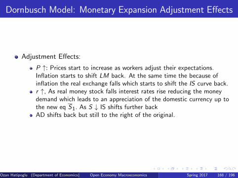
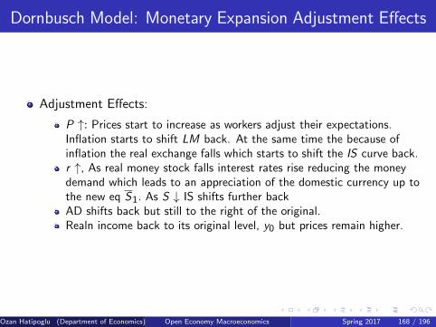
Adjustment Effects:
P ↑: Prices start to increase as workers adjust their expectations.Inflation starts to shift LM back. At the same time the because ofinflation the real exchange falls which starts to shift the IS curve back.r ↑, As real money stock falls interest rates rise reducing the moneydemand which leads to an appreciation of the domestic currency up tothe new eq S1. As S ↓ IS shifts further backAD shifts back but still to the right of the original.Realn income back to its original level, y0 but prices remain higher.
Ozan Hatipoglu (Department of Economics) Open Economy Macroeconomics Spring 2017 168 / 196
Dornbusch Model: Monetary Expansion Adjustment Effects
Adjustment Effects:
P ↑: Prices start to increase as workers adjust their expectations.Inflation starts to shift LM back. At the same time the because ofinflation the real exchange falls which starts to shift the IS curve back.
r ↑, As real money stock falls interest rates rise reducing the moneydemand which leads to an appreciation of the domestic currency up tothe new eq S1. As S ↓ IS shifts further backAD shifts back but still to the right of the original.Realn income back to its original level, y0 but prices remain higher.
Ozan Hatipoglu (Department of Economics) Open Economy Macroeconomics Spring 2017 168 / 196
Dornbusch Model: Monetary Expansion Adjustment Effects
Adjustment Effects:
P ↑: Prices start to increase as workers adjust their expectations.Inflation starts to shift LM back. At the same time the because ofinflation the real exchange falls which starts to shift the IS curve back.r ↑, As real money stock falls interest rates rise reducing the moneydemand which leads to an appreciation of the domestic currency up tothe new eq S1. As S ↓ IS shifts further back
AD shifts back but still to the right of the original.Realn income back to its original level, y0 but prices remain higher.
Ozan Hatipoglu (Department of Economics) Open Economy Macroeconomics Spring 2017 168 / 196
Dornbusch Model: Monetary Expansion Adjustment Effects
Adjustment Effects:
P ↑: Prices start to increase as workers adjust their expectations.Inflation starts to shift LM back. At the same time the because ofinflation the real exchange falls which starts to shift the IS curve back.r ↑, As real money stock falls interest rates rise reducing the moneydemand which leads to an appreciation of the domestic currency up tothe new eq S1. As S ↓ IS shifts further backAD shifts back but still to the right of the original.
Realn income back to its original level, y0 but prices remain higher.
Ozan Hatipoglu (Department of Economics) Open Economy Macroeconomics Spring 2017 168 / 196
Dornbusch Model: Monetary Expansion Adjustment Effects
Adjustment Effects:
P ↑: Prices start to increase as workers adjust their expectations.Inflation starts to shift LM back. At the same time the because ofinflation the real exchange falls which starts to shift the IS curve back.r ↑, As real money stock falls interest rates rise reducing the moneydemand which leads to an appreciation of the domestic currency up tothe new eq S1. As S ↓ IS shifts further backAD shifts back but still to the right of the original.Realn income back to its original level, y0 but prices remain higher.
Ozan Hatipoglu (Department of Economics) Open Economy Macroeconomics Spring 2017 168 / 196
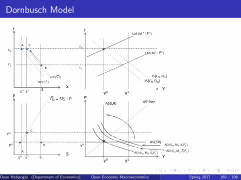
Dornbusch Model
r
S
r0
A
r
y0y
IS(G0,Q0)
P
S
B
P
y0y
450 line
y0P0
0( )RP S
0S
0 0( / )LM M P
*0 0 /Q SP P=
AS(LR)
AS(SR)
*0 0 0 0( , , )AD G M S P
1 0( / )LM M P
r1 r1
r0
1( )RP S
1S
0S
1S
P1
B
C
A
C
IS(G0,Q1)
y1
y1
*0 0 1 0( , , )AD G M S P
1S
1S
*0 0 1 0( , , )AD G M S P
Ozan Hatipoglu (Department of Economics) Open Economy Macroeconomics Spring 2017 169 / 196
Dornbusch Model: A Solution Algorithm
1. Determine the LR equilibrium S after the policy shock. Determinethe price level and real income in the LR ( Final Phase)
2. Using Dornbusch specification determine today’s exchange ratesand expected depreciation. Find the effects on IS, LM, AD , P.(Impact Phase)
3. Find out how variables above adjust as AS becomes vertical.(Adjustment Phase)
Ozan Hatipoglu (Department of Economics) Open Economy Macroeconomics Spring 2017 170 / 196
Recommended