DOCUMENT RESUME
ED 212 682 TM 820 254
AUTHOR Burkheimer, Graham J.; Jaffe, JayTITLE Highly Able Students Who Did Not Go To College.
Contractor Report.INSTITUTION Research Triangle Inst., Durham, N.C. Center for
Educational Research and Evaluation.SPONS AGENCY National Center for Educational Statistics (ED),
Washington, D.C.REPORT NO NCES-82-217PUB DATE Aug 81CONTRACT 0E-0-73-6666NOTE 76p.AVAILABLE FROM Superintendent of Documents, U.S. Government Printing
Office, Washington, DC 20402.
EDRS PRICE MF01/PC04 Plus Postage.DESCRIPTORS *Academic Ability; Academic Aspiration; *College
Attendance; Comparative Analysis; Higher Education;*High School Graduates; *Noncollege Bound Students;Secondary Education; Student Characteristics
IDENTIFIERS *National Longitudinal Study High School Class1972
ABSTRACTThe data collected from the in-school and three
follow-up surveys of the National Longitudinal Study of the HighSchool Class of 1972 have been merged and processed. Results arebeing presented in a series of reports designed to highlight selectedfindings in educational, career, and occupational development. Thisreport focuses on students who were in the top quarter of theirgraduating class in academic ability but who had not entered collegefour and one-half years after high school graduation. In particular,the report presents information about the potential reasons fornonattendance and the current activity states of these highly ablestudents. For comparison purposes, results are also presented forthose of other ability levels. Study findings indicate that theeffects on and of college attendance are basically similar for allability levels. Where differences exist, they are quantitative ratherthan qualitative, suggesting that similar factors affect and areaffected by college attendance but that they operate and are operatedupon to a different extent for the highly able student.(Author/GIC)
************************************************************************ Reproductions supplied by EDRS are the best that can be made *
* from the original document. *
***********************************************************************
(4
;$.
I.4
Highly Able Students Who Did Not Go ToCollege
Center for Educational Research and Evaluation
Graham J. BurkheimerJay Jaffe
Andrew J. KolstadProject OfficerNational Center for Education Statistics
August 1981
Prepared for the National Center for EducationStatistics under contract OE-0-73-6666 with theU.S. Department of Fducation. Contractors under-taking such projects are encouraged to expressfreely their professional judgment. This repo :t.therefore. does not necessarily represent position.,on policies of the Government. and no officialendorsement >tmid he inferred. This report isreleased as received from the contractor.
NCES 82.217
For sale by the Superintendent of Documents, U.S. Government Printing OfficeWashington, D.C. 20402
FOREWORD
The National Longitudinal Study of the High School Class of 1972, a
survey initiated by and conducted for the National Center for Education Sta-
tistics (NCES), began in spring 1972 with over 1,000 in-school group admin-
istrations of survey forms to a sample of approximately 18,000 seniors. In
the several follow-up surveys, the sample included almost 5,000 additional
students from sample schools that were unable to participate in the base-year
survey.
The data collected from the in-school and three follow-up surveys have
been merged and processed. Results are being presented in a series of reports
designed to highlight selected findings in educational, career, and occupa-
tional development. This report focuses on students who were in the top
quarter of their graduating class in academic ability but who had not entered
coll!ge four and one-half years after high school graduation. In particular,
the report presents information about the potential reasons for nonattendance
and the current activity states of these highly able students. For comparison
purposes, results are also presented for those of other ability levels.
David Sweet, Director C. Dennis Carroll, ChiefDivision of Multilevel Education Longitudinal Studies BranchStatistics NCES
NCES
iii
ACKNOWLEDGEMENTS
The authors wish to thank all those people who have contributed to the
writing of this report. In particular, acknowledgement is due to Mr. William
B. Fetters of the National Center for Education Statistics, who was the prin-
cipal NCES staff member responsible for supervising the preparation of the
report and whose many valuable suggestions were a major force in shaping the
final report. Acknowledgements are also due to Dr. Andrew Kolstad, current
NCES Project Officer, Dr. Bruce K. Eckland of the University of North Carolina
at Chapel Hill, and Dr. J. R. Levinsohn, former NLS Project Director at the
Research Triangle Institute for their considerable input and assistance.
Dr. George Dunteman of RTI, as well as Dr. John Riccobono, NLS Fourth
Follow-up Project Director, reviewed earlier drafts of the present report and
changes thereto. Special thanks also are due to Ms. Cecille Stafford,
Ms. Linda Hoffman, Ms. Gail Bisplinghoff, Ms. Pam Mikels and Ms. Barbara
Elliott for their assistance is the preparation of the manuscript.
A final word of acknowledgement and an expression of gratitude is due to
the mny persans in the Federal government and at RTI who assisted in planning
and implementing the National Longitudinal Study of the High School Class of
1972; to the more than 20,000 young adults who took the time and effort to
provide comprehensive, detailed information about their lives; and to the
participating high schools that made it possible to initiate the study in
1972.
v
ABSTRACT
Recent surveys indicate that a large proportion (more than one in five)
of students in the top ability quartile of the high school graduating class do
not attend college. Due to the implications of this talent loss, at both the
individual and national level, this study was initiated in an attempt to
identify factors related to college attendance by able students and to see how
highly able students who did not attend college fare in the world of work.
For comparison, low and middle ability groups also were considered.
In modeling college attendance, five major constructs were considered:
individual and family background factors, high school academic credentials,
educational expectations, life values, and early marriage. The five con-
structs jointly accounted for only about one-third of the variation in college
attendance of high ability (or other ability level) students. Of the con-
structs, only the life values variable set (as measured by three fairly weak
scales) failed to show a unique relationship to college attendance at any
ability level. For the remaining constructs, the factors related to college
attendance for highly able students were generally similar to and direction-
ally consistent with those for other ability groups. Some differential rela-
tionships were observed among the three ability levels, but they typically
reflected only a difference in the extent to which a factor was associated
with college attendance.
Low educational expectation was the strongest unique predictor of college
nonentry among high ability students; this factor alone accounted for roughly
30 percent of the variation in college going. Educational expectation was
also the strongest predictor of college going at other ability levels, but was
markedly less predictive for low ability students than for the high or middle
ability groups. Early marriage also was strongly related to not attending
college, and the effect was about twice as large for the highly able as for
other ability levels.
As a group, the academic credential variable., also were quite predictive
of college going; of the four variables in this set, only number of high
school science courses showed no unique relationship at any ability level.
Lower high school class rank and fewer high school math courses characterized
the highly able noncollege group, and these relationships did not differ
statistically from those for other ability groups. A nonacademic high school
vii
program was a strong unique predictor of college nonentry for middle and low
ability students, but no such direct effect was observed for the highly able.
When considering indirect effects, however, high school program was also
predictive for the high ability group.
Among the background factors, race/ethnicity was consistently nonpre-
dictive of college entry regardless of ability level. Sex was predictive only
for the highly able. When other variables were controlled, highly able males
were less likely to attend college than females; however, when indirect
effects were considered, the female advantage in attendance was reversed.
Lower socioeconomic status also signaled a decreased likelihood of attending
college for the highly able, but the effect was over twice as great for the
middle ability group than for either of the extreme ability groups (high or
low).
In examining other life outcomes as potential consequences of ability and
college attendance, family formation indices and job outcomes four ano a half
years after high school graduation were considered. Results indicate some
group differences, but the differences were related more strongly to college
attendance than to ability. Only one major difference in family formation
existed between highly able students who did not go to college and noncollege
groups of less ability; the highly able were less likely to have become
parents. Family formation indices did show clearcut and fairly intuitive
differences as a function of college entry (highly able students not attending
college had married at about twice the rate and had become parents at about
five times the rate of their college-going counterparts), but such differences
are obviously timebound.
The examination of job outcomes indicated few differences as a function
of either college attendance or ability level; however, these results should
be considered inconclusive, since the time point examined represents a very
early point in the career of these young people, particularly those who at-
tended college (in fact, many were still in college and thus unrepresented in
the job outcome analyses). The major difference within the noncollege group
was that those of high ability were more likely than those of middle or low
ability to have aspired to (as high school seniors) and to have attained (by
October 1976) a professional or technical career; however, at all ability
levels college goers were much more likely than nongoers to have both aspired
to and attained such careers. Those highly able students who had not attended
viii 7

college defined themselves out of the work force at about twice the rate of
those who had attended, but did not differ in this respect from noncollege
groups of lower ability. Of those in the work force, employment rates did not
differ as a function of college going or ability, and there were no systematic
differences between the college and noncollege groups or among ability levels
in hours worked, earnings, or job satisfaction.
ix
8

CONTENTS
Foreword iii
Acknowledgements v
Abstract vii
I. Introduction1
A. Background and Purpose of the Study 1
B. Data Source 2
C. Weighting and Significance Testing 3
D. An Overview of the Report 5
II. Reasons for College Nonattendance 5
A. Conceptualization 6
B. Measurement Specifications 7
C. Comparisons of the College and Noncollege Groups 10
D. Simultaneous Prediction of College Attendance 14
E. Modeling College Attendance 23
III Activities in 1976 27
A. Family Formation 27
B. Job Attainment 30
C. Job Satisfaction 36
IV. Summary and Discussion 38
A. Potential Determinants of College Attendance 38
B. Consequences of College Nonattendance 40
References 43
Appendix A. Supplementary Tables 45
xi 9
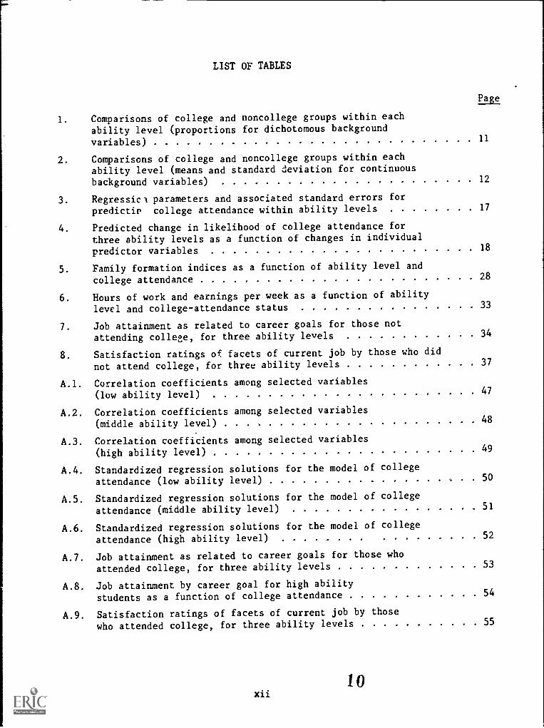
LIST OF TABLES
Page
1. Comparisons of college and noncollege groups within eachability level (proportions for dichotomous backgroundvariables) 11
2. Comparisons of college and noncollege groups within eachability level (means and standard deviation for continuousbackground variables) 12
3. Regressicl parameters and associated standard errors forpredictir college attendance within ability levels 17
4. Predicted change in likelihood of college attendance forthree ability levels as a function of changes in individual
predictor variables 18
5. Family formation indices as a function of ability level and
college attendance 28
6. Hours of work and earnings per week as a function of ability
level and college-attendance status 33
7. Job attainment as related to career goals for those not
attending college, for three ability levels 34
8. Satisfaction ratings of facets of current job by those who did
not attend college, for three ability levels 37
A.1 Correlation coefficients among selected variables
(low ability level) 47
A.2. Correlation coefficients among selected variables
(middle ability level) 48
A.3. Correlation coefficients among selected variables
(high ability level) 49
A.4. Standardized regression solutions for the model of college
attendance (low ability level) 50
A.S. Standardized regression solutions for the model of college
attendance (middle ability level) 51
A.6. Standardized regression solutions for the model of college
attendance (high ability level) 52
A.7. Job attainment as related to career goals for those who
attended college, for three ability levels 53
A.8. Job attainment by career goal for high abilitystudents as a function of college attendance 54
A.9. Satisfaction ratings of facets of current job by those
who attended college, for three ability levels 55
10xii
LIST OF FIGURES
Page
1. A general model of college attendance 8
2. Path analytic solution of the model for college attendance 25
J. Employment status by ability category and college attendance. 31
i
11
I. INTRODUCTION
A. Background and Purpose of the Study
Educational and occupational development of young people has always been
an important concern to educators and policymakers. A number of studies have
been conducted over the years to identify factors that are related to young
people's entry into higher education and their .lbsequent educational and
occupational attainment (e.g., Astir,, 1965; Bailey and Collins, 1977; Bowers,
et al., 1977; College Entrance Examination Board, 1974; Thomas et al., 1977).
These studies have been particularly concerned with the equality of educa-
tional opportunities for women, ethnic minorities, and students of low socio-
economic status (SES). Social pressures, government assistance, and the
efforts cf individual institutions have been directed toward making college
more available to less advantaged youths, and several recent studies have
shown that differences in access to higher education have been narrowing
between men and women, as well as among SES and ethnic groups (cf., Peng, et
al., 1977).
Recent studies also have shown repeatedly that a large proportion of
highly able students do not go to college (Peng, 1977). For example, over 22
percent of the 1972 high school class (about 20 percent of the men and 25
percent of the women) who were in the top ability quartile did not attend
college during the four and one-half years after high school graduation. In
terms of personal development and subsequent use of their talents, and in
terms of enhancing the development of our nation's manpower resources, ad-
vanced technologies, skills, and knowledge, it would seem desirable for those
able students to enter college and complete a higher education degree.
Studies have shown, in fact, that the proportion of highly able young men
entering college has declined, although there has been an increase in the rate
of college entry among able women in the lowest SES quartile (Peng, 1977).
Thus, it seems appropriate to ask why so many able students do no go to
college. Is it because of the lack of financial support or inadequate aca-
demic preparation? Is it because of the lack of motivation for higher edu-
cation as a result of factors such as a tight labor market for college grad-
uat-s or a career choice that does not require a college eduction? Are the
factors related to college attendance among able students the same as those
12
for students of other ability levels? It also seems appropriate to ask what
eventually happens to the highly able students who do not go to college. Do
they find ways to put their talents to social and personal use? How different
are they, with respect to early career attainment and family life, from those
of other ability levels who did not attend college and from highly able
students who entered college?
This report is intended to address these questions. Answers to the set
of questions concerning college attendance could help to reveal barriers to
higher education among able students. Answers to the questions of early
career attainment could help in evaluating the extent to which an able
student's talent is lost if he does not attend college, and could also yield
some evidence regarding the value of a college education. It should be noted
that, while the first set of questions can be adequately addressed with the
current data, the second set of questions (particularly those involving the
college-going group) can be addressed fully only with data that cover a longer
period of time. Nonetheless, the present study can provide preliminary sug-
gestions of early career attainment and family life.
B. Data Source
The data for this study were drawn from the National Longitudinal Study
of the High School Class of 1972 (NLS). Sponsored by the National Center for
Education Statistics, the NLS is a long-term educational research program.
Its mission is to discover what happens to young people after they leave high
school, as measured by their subsequent educational and vocational activities,
plans, aspirations, and attitudes, and to relate this information to their
prior personal and educational experiences.
The full-scale study began in the spring of 1972. A national probability
sample of over 19,000 seniors from 1,061 public, private, and church-affili-
ated high schools was selected, and over 18,000 of those seniors participated
in the base-year survey. Each student was asked to complete a student ques-
tionnaire and a 69-minute test battery. Background information for each
student plus information about the schoui's programs, resources, and grading
system also was collected from school records. In addition, school counselors
were asked to complete a special questionnaire designed to provide data about
their training and experience.
13
The first follow-up survey was conducted from October 1973 to April 1974.
Added to the base-year sample were about 4,450 students of the class of 1972
from 249 additional high schools that had been unable to participate earlier.
Some 21,350 young people completed a First Follow-Up Questionnaire. A second
follow-up survey was conducted from October 1974 to April 1975, and 20,872
young people completed the survey questionnaire. The third follow-up survey
was conducted from October 1976 to April 1977, and 20,092 persons completed
the survey questionnaire.
Although the primary focus of this study is on highly able students,
analyses have considered students of other ability levels for the purpose of
comparison. Of the total NLS base-year participants with available test
scores, 4,052 were in the top quarter, 7,000 in the middle two quarters, and
4,788 in the bottom quarter of general academic ability.1/
C. Weighting and Significance Testing
The NLS data base results from a highly stratified, multistage cluster
sample. Each case must therefore be weighted by the inverse of its proba-
bility of selection to obtain unbiased estimates of population parameters.
The percentages, means, and sL..ndard deviations presented in this report are
all based upon properly weighted estimates. The standard errors of sample
statistics from this complex design are larger than those obtained in a random
sample. For example, standard errors of proportions can be approximated as a
function of the estimated proportion, the sample size, and the estimated
design effect (i.e., the ratio of the sampling variance of the statistic for
this sample to the sampling variance of the statistic for a simple random
sample of the same size). Approximate standard error of proportions in this
report can be obtained by the following equation,
1/
The academic ability index was derived from a standardized composite offour base-year test scores: Vocabulary, Reading, Letter Groups, and Mathe-matics. The cutting points for defining quartiles were based on a weightedestimate of the test score composite mean and standard deviation, and theassumption that the weighted frequency distribution was normal. Because lowSES students were oversampled and SES is correlated with ability, more than 25percent of the unweighted number of sample members actually fell into the lowquartile of the ability composite.
3
14
S.E.(p) = P(1 -P) Dn
where p is the proportion, D is the design effect, and n is the actual sample
size. AlLlogous expressions exist for standard errors of means, expressed in
terms of standard deviations, n, and D (see Kish, 1957; Kish and Frankel,
1970). The general design effect for proportions in this study is estimated
to be approximately 1.35; thus, the usual standard errors should be multiplied
by F175, about 7.16.
To contrast two subpopulation proportions, d = p1 - p2, the standard
error of the difference is approximated by taking the square root of the sum
of the squares of the standard errors for p1 and p2. This approximation does
not account for the subtraction of the covariance term for p1 and p2 in the
estimation formula; however, in comparing two subclasses of students, the
covariance term tends to be positive because of the positive correlation
introduced by the sample clusters of 18 students per school. Since the effect
of such a positive correlation would be to reduce the standard error of the
difference, the suggested approximation typically will be conservative.
It should be noted that the significance tests of proportions and propor-
tion differences employed in this report are based on the normal approximation
to the binominal distribution, which is based on assumptions that may not hold
for small sample sizes or extreme proportions. Further, while standard errors
for means, proportions, and differences in means and proportions did account
for the general design effect (see above), exact standard errors (incorpor-
ating effects of stratification and clustering for the specific statistic
under consideration) were not computed. As such, it is appropriate, as a
general rule, to interpret reported standard errors as somewhat nonconser-
vative. For regression solutions, design effects were not incorporated in
analysis; consequently, reported standard errors for various regression and
correlation parameter estimates are even more likely to be nonconservative.
Because of the large sample sizes, the number of statistics reported, and the
suspected nonconservative nature of standard errors, a .01 level of Type I
error probability is used throughout as the criterion for statistical signif-
icance.
15
D. An Overview of the Report
The remainder of this report is organized into three sections. Sec-tion II focuses on the question of why many highly able students did not go tocollege. The presentation includes a conceptualization of the problem, spec-ifications of measurement, and the results of three approaches to analysis.Section III examines the current activities of highly able individuals, with afocus on their job attainment, job satisfaction, and family formation. Themajor findings are summarized and discussed in Section IV. Supplementaryresults, included in Appendix A, are appropriately referenced in the text.
5
16
II. REASONS FOR COLLEGE NONATTENDANCE
A. Conceptualization
As indicated earlier, a substantial proportion of highly able students of
the class of 1972 did not go to college; about 22 percent of students who were
in the top quarter of academic ability had not attended college in the four
and one-half years following high school graduation. A logical extension of
investigation is to inquire why such able students did not go to college.
General factors influencing college nonattendance such as low socioeconomic
status and inadequate academic credentials, as determined from the entire NLS
data base (see Peng, Bailey, and Eckland, 1977) may be equally applicable to
the subset of highly able students. On the other hand, the factors associated
with college attendance in the highly able group may differ, qualitatively or
quantitatively, from those operating at other abi'ity levels. To investigate
these issues, several sets of analyses were conducted using three ability
groups: (1) students in the top quarter of general academic ability (i.e.,
highly able students); (2) students in the middle two quarters; and (3) stu-
dents in the bottom quarter.-2/
Regardless of ability level, entry into college is assumed to be a com-
plex process, involving a number of such interrelated individual factors as
academic credentials for college, social and economic deprivation, and moti-
vation or interest.2/ A fair number of the highly able young people simply
may have never obtained the academic credentials for attending college due to
factors such as failure to enroll in a college preparatory curriculum in high
school or having a low class rank. In addition to credential inadequacy, it
is possible that many of those not attending might have had more social or
economic handicaps than their counterparts who attended college. It is also
likely that many highly able students simply did not aspire to college; some
might have been oriented toward occupational success in areas for which they
1/ This quartile classification was derived from an ability composite computed
from base-year test data (cf., Dunternan, Peng and Holt, 1974; Levinsohn et
al., 1978, Appendix 0).
2/ Other contextual factors could be considered such as formal and informal
counseling on college entrance and available financial aid, or entry require-
ments of specific colleges to which application may have been made. While
such factors were not examined directly, they are probably reflected to vary-ing extents in the variables considered.
17
believed that a college education would not increase their opportunities.
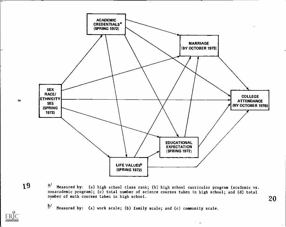
Of course, these factors may be interrelated, and such relationships need
to be explicated. One model attempting to describe these interrelationships
is presented in Figure 1. The ordering of the variables is dictated by a
hypothesized causal structure linking one variable with another or by temporal
considerations. The longitudinal nature of the data base is a strong feature
of the study, since the temporal sequence of variables allows a more defensi-
ble explanation of process variables that affect college entry.
The model assumes that college attendance of highly able students, and
other students as well, is a result of the direct or indirect "influence" or
"effect" of social background (sex, race/ethnicity, SES), academic creden-
tials, life values, educational aspirations, and marital status. Some of
these influences are also assumed to be mediated through other variables.
B. Measurement Specifications
Variables involved in the model are specified as follows:
(1) Sex: Female was assigned a value of 1; and male, 0.
(2) Race/ethnicity: Majority white was assigned a value of 1; and all
minorities, 0.
(3) Socioeconomic Status (SES): SES was based upon a composite of base-
year data on father's education, mother's education, parental in-
come, father's occupation, and a household items index. Factor
analysis, in wnich missing components were imputed as the mean of
the subpopulation of which the respondent was a member (defined
according to cross-classification of race/ethnicity, high school
program, and aptitude), revealed a coy on factor with approximately
equal loading for each of the five components. As a result of the
suggested equal component weighting, avail.: (nonimputed) stan-
dardized components were averaged to form an score, when at
least two nonimputed components were available. A high s re indi-
cates a high SES (see Dunteman, et al., 1974).
(4) Academic Credentials: The variables used as measures were:
(a) High School Class Rank: Student percentile rank obtained from
the school record information.
(b) High School Curriculum Program: Based on student questionnaire
information, students in college preparatory (academic) pro-
grams were assigned a value of 1, and those in general voca-
tional or technical programs were assigned a value of 0.
7
18
19
SEXRACE/
ETHNICITYSES
(SPRING1972)
ACADEMICCREDENTIALS(SPRING 1972)
,11111,11MARRIAGE
(BY OCTOBER 1973)
LIFE VALUESb(SPRING 1972)
EDUCATIONALEXPECTATION(SPRING 1972)
COLLEGEATTENDANCE
(BY OCTOBER 1976)
a/Measured by: (a) high school class rank; (b) high school curricular program (academic vs.
nonacademic program); (c) total number of science courses taken in high school; and (d) totalnumber of math courses taken in high school.
12/ Measured by: (a) work scale; (b) family scale; and (c) community scale.
20
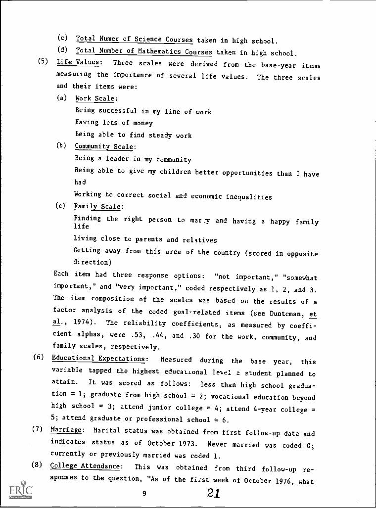
(c) Total Numer of Science Courses taken in high school.
(d) Total Number of Mathematics Courses taken in high school.
(5) Life Values: Three scales were derived from the base-year items
measuring the importance of several life values. The three scales
and their items were:
(a) Work Scale:
Being successful in my line of work
Having lets of money
Being able to find steady work
(b) Community Scale:
Being a leader in my community
Being able to give my children better opportunities than I havehad
Working to correct social and economic inequalities
(c) Family Scale:
Finding the right person to marry and having a happy familylife
Living close to parents and relatives
Getting away from this area of the country (scored in opposite
direction)
Each item had three response options: "not important," "somewhat
important," and "very important," coded respectively as 1, 2, and 3.
The item composition of the scales was based on the results of a
factor analysis of the coded goal-related items (see Dunteman, etal., 1974). The reliability coefficients, as measured by coeffi-cient alphas, were .53, .44, and .30 for the work, community, andfamily scales, respectively.
(6) Educational Expectations: Measured during the base year, this
variable tapped the highest educational level a student planned to
attain. It was scored as follows: less than high school gradua-
tion = 1; graduate from high school = 2; vocational education beyondhigh school = 3; attend junior college = 4; attend 4-year college =
5; attend graduate or professional school = 6.
(7) Marriage: Marital status was obtained from first follow-up data andindicates status as of October 1973. Never married was coded 0;
currently or previously married was coded 1.
(8) College Attendance: This was obtained from third follow-up re-
sponses to the question; "As of the first week of October 1976, what
9 21
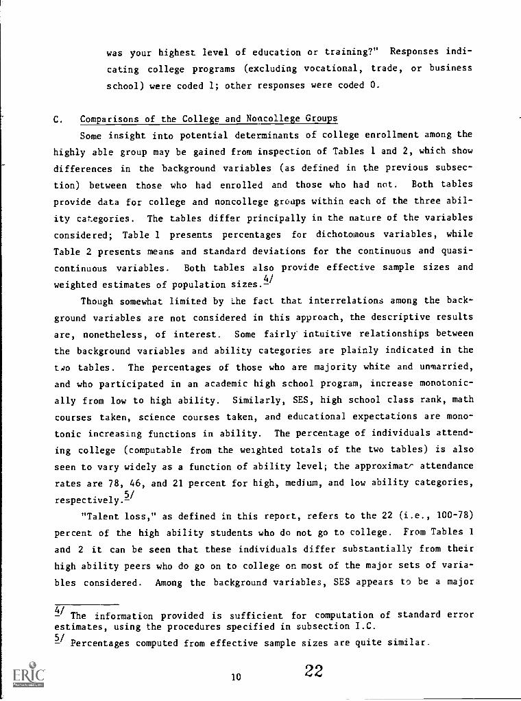
was your highest level of education or training?" Responses indi-
cating college programs (excluding vocational, trade, or business
school) were coded 1; other responses were coded 0.
C. Comparisons of the College and Noncollege Groups
Some insight into potential determinants of college enrollment among the
highly able group may be gained from inspection of Tables 1 and 2, which show
differences in the background variables (as defined in the previous subsec-
tion) between those who had enrolled and those who had not. Both tables
provide data for college and noncollege groups within each of the three abil-
ity categories. The tables differ principally in the nature of the variables
considered; Table 1 presents percentages for dichotomous variables, while
Table 2 presents means and standard deviations for the continuous and quasi-
continuous variables. Both tables also provide effective sample sizes and
weighted estimates of population sizes.4/
Though somewhat limited by :.he fact that interrelations among the back-
ground variables are not considered in this approach, the descriptive results
are, nonetheless, of interest. Some fairly' intuitive relationships between
the background variables and ability categories are plainly indicated in the
two tables. The percentages of those who are majority white and unmarried,
and who participated in an academic high school program, increase monotonic-
ally from low to high ability. Similarly, SES, high school class rank, math
courses taken, science courses taken, and educational expectations are mono-
tonic increasing functions in ability. The percentage of individuals attend-
ing college (computable from the weighted totals of the two tables) is also
seen to vary widely as a function of ability level; the approximate attendance
rates are 78, 46, and 21 percent for high, medium, and low ability categories,
respectively.
"Talent loss," as defined in this report, refers to the 22 (i.e., 100-78)
percent of the high ability students who do not go to college. From Tables 1
and 2 it can be seen that these individuals differ substantially from their
high ability peers who do go on to college on most of the major sets of varia-
bles considered. Among the background variables, SES appears to be a major
/The information provided is sufficient for computation of standard error
estimates, using the procedures specified in subsection I.C.
Percentages computed from effective sample sizes are quite similar.
10 22
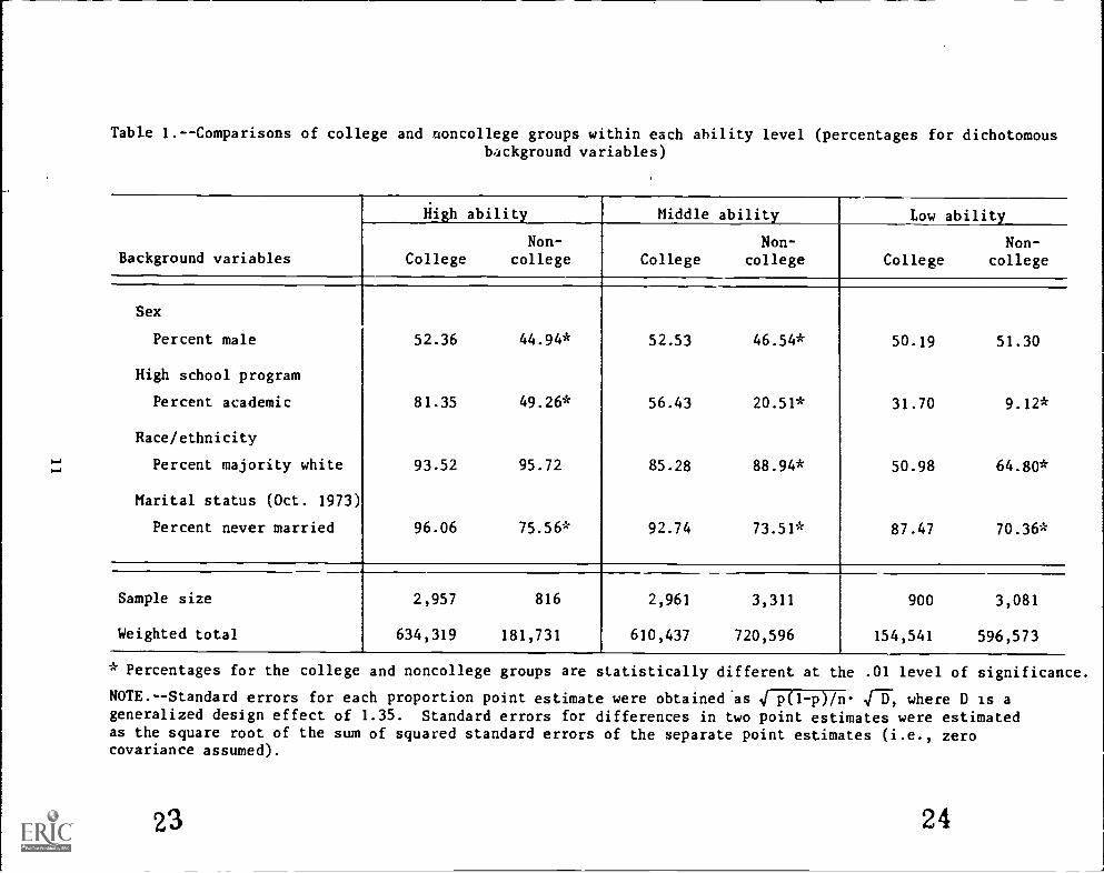
Table 1.--Comparisons of college and uoncollege groups within each ability level (percentages for dichotomousbackground variables)
Background variables
High ability Middle ability Low ability
CollegeNon-
college CollegeNon-
collegeNon-
College college
Sex
Percent male 52.36 44.94* 52.53 46.54* 50.19 51.30
High school program
Percent academic 81.35 49.26* 56.43 20.51* 31.70 9.12*
Race/ethnicity
Percent majority white 93.52 95.72 85.28 88.94* 50.98 64.80*
Marital status (Oct. 1973)
Percent never married 96.06 75.56* 92.74 73.51* 87.47 70.36*
Sample size 2,957 816 2,961 3,311 900 3,081
Weighted total 634,319 181,731 610,437 720,596 154,541 596,573
* Percentages for the college and noncollege groups are statistically different at the .01 level of significance.
NOTE.--Standard errors for each proportion point estimate were obtained'as 4 p(1-p)/n [1, where D is ageneralized design effect of 1.35. Standard errors for differences in two point estimates were estimatedas the square root of the sum of squared standard errors of the separate point estimates (i.e., zerocovariance assumed).
23 24
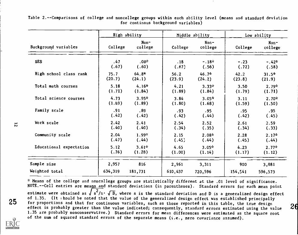
Table 2.--Comparisons of college and noncollege groups within each ability level (means and standard deviationfor continous background variables)
High ability Middle ability Low ability
Non-Non- Non-BackgrouRd variables College college College college College college
SES .47 .00* .18 -.18* -.23 -.42*(.67) (.60) (.67) (.56) (.72) (.58)
High school class rank 75.7 64.8* 56.2 46.7* 42.2 31.5*(20.7) (24.1) (23.9) (24.2) (23.8) (21.9)
Total math courses 5.18 4.16* 4.21 3.33* 3.50 2.79*(1.71) (1.84) (1.89) (1.84) (1.79) (1.71)
Total science courses 4.73 3.95* 3.84 3.05* 3.11 2.70*(1.159) (1.89) (1.80) (1.68) (1.59) (1.50)
Family scale .91 .89 .93 .95 .95 .95(.42) (.42) (.42) (.44) (.42) (.45)
Work scale 2.42 2.41 2.54 2.52 2.61 2.59(.40) (.40) (.34) (.35) (.34) (.33)
Community scale 2.04 1.99* 2.15 2.08* 2.28 2.17*(.47) (.44) (.45, (.44) (.45) (.44)
Educational expectation 5.12 3.61* 4.65 3.05* 4.23 2.77*(.76) (1.28) (1.00) (1.14) (1.17) (1.12)
Sample size 2,957 816 2,961 3,311 900 3,081
Weighted total 634,319 181,731 610,437 720,596 154,541 596,573
* Means of the college and noncollege groups are statistically different at the .01 level of significance.NOTE.--Cell entries are means and standard deviations (in parentheses). Standard errors for each mean point
estimate were obtained as s2/n 4-6, where s is the standard deviation and D is a generalized design effect
of 1.35. (It :hould be noted that the value of the generalized design effect was established principallyfor proportions and that for continuous variables, such as those reported in this table, the true designeffect is probably greater than the value indicated; consequently, standard errors estimated using the value1.35 are probably nonconservative.) Standard errors for mean differences were estimated as the square rootof the sum of squared standard errors of the separate means (i.e., zero covariance assumed).
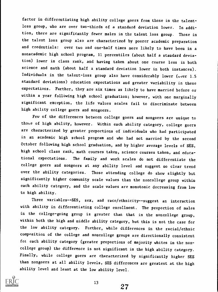
factor in differentiating high ability college goers from those in the talent-
loss group, who are over two-thirds of a standard deviation lower. In addi-
tion, there are significantly fewer males in the talent loss group. Those in
the talent loss group also are characterized by poorer academic preparation
and credentials: over two and one-half times more likely to have been in a
nonacademic high school program, 11 percentiles (about half a standard devia-
tion) lower in class rank, and having taken about one course less in both
science and math (about half a standard deviation lower in both instances).
Individuals in the talent-loss group also have considerably lower (over 1.5
standard deviations) education expectations and greater variability in these
expectations. Further, they are six times as likely to have married before or
within a year following high school graduation; however, with one marginally
significant exception, the life values scales fail to discriminate between
high ability college goers and nongoers.
Few of the differences between college goers and nongoers are unique to
those of high ability, however. Within each ability category, college goers
are characterized by greater proportions of individuals who had participated
in an academic high school program and who had not married by the second
October following high school graduation, and by higher average levels of SES,
high school class rank, math courses taken, science courses taken, and educa-
tional expectations. The family and work scales do not differentiate the
college goers and nongoers at any ability level and suggest no clear trend
over the ability categories. Those attending college do show slightly but
significantly higher community scale values than the noncollege group within
each ability category, and the scale values are monotonic decreasing from low
to high ability.
Three variables--SES, sex, and race/ethnicity--suggest an interaction
with ability in differentiating college enrollment. The proportion of males
in the college-going group is greater than that in the noncollege group,
within both the high and middle ability category, but this is not the case for
the low ability category. Further, while differences in the racial/ethnic
composition of the college and noncollege groups are directionally consistent
foi each ability category (greater proportions of majority whites in the non-
college group) the difference is not significant in the high ability category.
Finally, while college goers are characterized by significantly higher SES
than nongoers at all ability levels, SES differences are greatest at the high
ability level and least at the low ability level.
13
27
On balance, these descriptive results suggest that, in general, similar
factors are associated with college going regardless of ability level, al-
though not necessarily to the same extent, even though these factors also vary
with ability. Compared to college goers, those who had not gone to college
have poorer academic credentials, hiLher rates of early marriage, lower educa-
tional expectations, and lower soci3economic status (in the latter case an
interaction with ability level is suggested). With the exception of the
community scale, the life value scales do not appear to be associated with
college going or ability level. Sex and race/ethnicity, on the other hand,
are not consistently associated with college going in all ability categories.
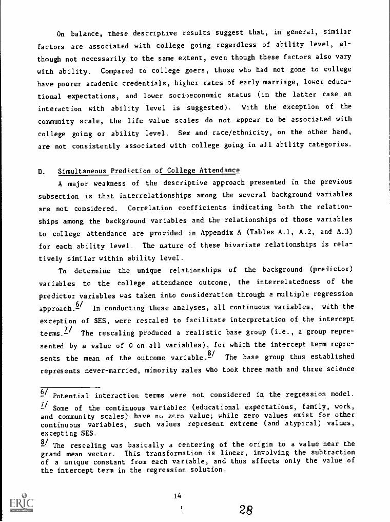
D. Simultaneous Prediction of College Attendance
A major weakness of the descriptive approach presented in the previous
subsection is that interrelationships among the several background variables
are not considered. Correlation coefficients indicating both the relation-
ships among the background variables and the relationships of those variables
to college attendance are provided in Appendix A (Tables A.1, A.2, and A.3)
for each ability level. The nature of these bivariate relationships is rela-
tively similar within ability level.
To determine the unique relationships of the background (predictor)
variables to the college attendance outcome, the interrelatedness of the
predictor variables was taken into consideration through a multiple regression
approach.-6/ In conducting these analyses, all continuous variables, with the
exception of SES, were rescaled to facilitate interpretation of the intercept
terms.1/ The rescaling produced a realistic base group (i.e., a group repre-
sented by a value of 0 on all variables), for which the intercept term repre-
sents the mean of the outcome variable.-11/ The base group thus established
represents never-married, minority males who took three math and three science
/ Potential interaction terms were not considered in the regression model.
/ Some of the continuous variables (educational expectations, family, work,
and community scales) have nu zcro value; while zero values exist for other
continuous variables, such values represent extreme (and atypical) values,
excepting SES.
8/ The rescaling was basically a centering of the origin to a value near the
grand mean vector. This transformation is linear, involving the subtraction
of a unique constant from each variable, and thus affects only the value of
the intercept term in the regression solution.
14
28
courses in a nonacademic high school program, who attained a high school class
rank of 50 percent, who expected to attend a junior college (unscaled value of
4), and who had composite scores of 0, 1, 2, and 2.5 on SES, family scale,
community scale, and work scale, respectively.
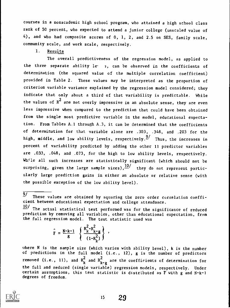
1. Results
The overall predictiveness of the regression model, as applied to
the three separate ability le. 3, can be observed in the coefficients of
determination (the squared value of the multiple correlation coefficient)
provided in Table 2. These values may be interpreted as the proportion of
criterion variable variance explained by the regression model considered; they
indicate that only about a third of that variability is predictable. While
the values of R2
are not overly impressive in an absolute sense, they are even
less impressive when compared to the prediction that could have been obtained
from the single most predictive variable in the model, educational expecta-
tion. From Tables A.1 through A.3, it can be determined that the coefficients
of determination for that variable alone are .303, .348, and .203 for the
high, middle, and low ability levels, respectively.2/ Thus, the increases in
percent of variability predicted by adding the other 11 predictor variables
are .033, .048, and .073, for the high to low ability levels, respectively.
While all such increases are statistically significant (which should not be
surprising, given the large sample sizes),10/
they do not represent partic-
ularly large prediction gains in either an absolute or relative sense (with
the possible exception of the low ability level).
9/These values are obtained by squaring the zero order correlation coeffi-
cient between educational expectation and college attendance.10/
The actual statistical test performed was for the significance of reducedprediction by removing all variables, other than educational expectation, fromthe full regression model. The test statistic used was
2 2
F =N-k-1 Rk-Rk-g
g 2(1-R )
where N is the sample size (which varies with ability level), k is the numberof predictions in the full model (i.e., 12), g is the number of predictors
2 2removed (i.e., 11), and Rk
and Rk-g
are the coefficients of determination for
the full and reduced (single variable) regression models, respectively. Undercertain assumptions, this test statistic is distributed as F with g and N-k-1degrees of freedom.
15 29
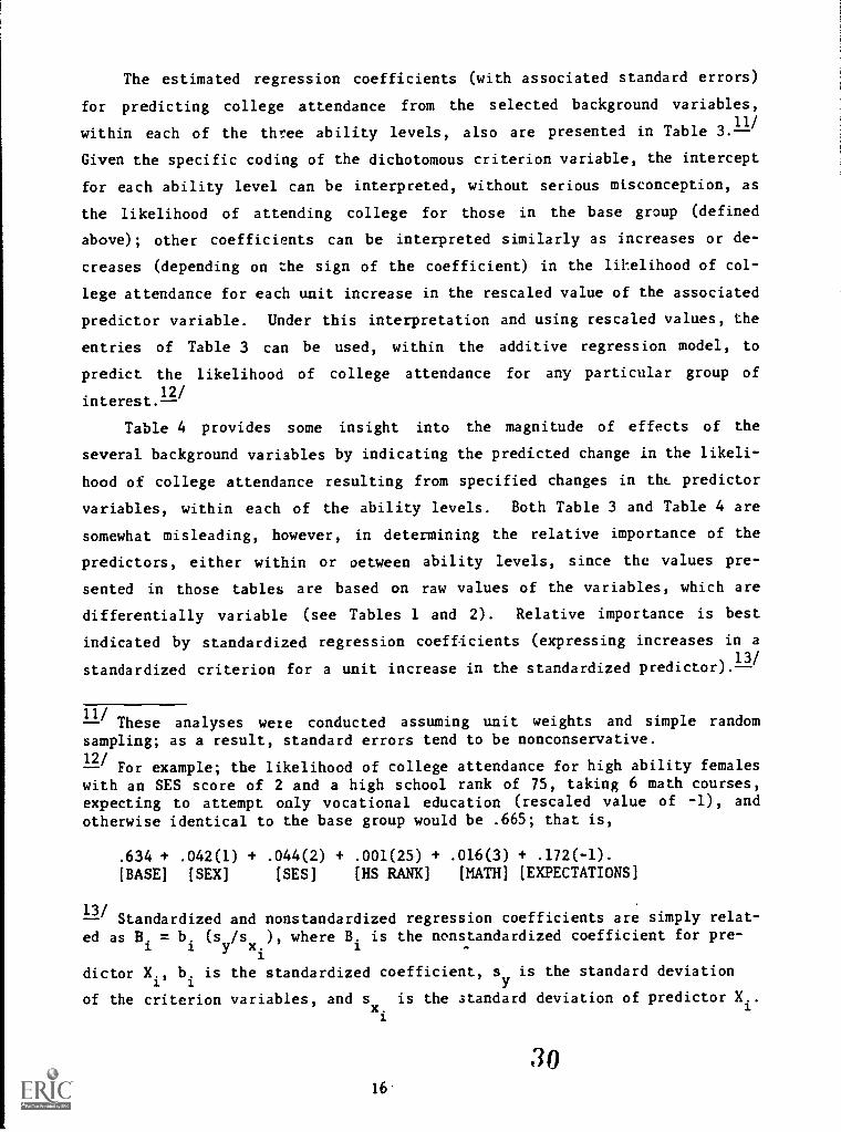
The estimated regression coefficients (with associated standard errors)
for predicting college attendance from the selected background variables,
within each of the three ability levels, also are presented in Table 3.11/
Given the specific coding of the dichotomous criterion variable, the intercept
for each ability level can be interpreted, without serious misconception, as
the likelihood of attending college for those in the base group (defined
above); other coefficients can be interpreted similarly as increases or de-
creases (depending on the sign of the coefficient) in the likelihood of col-
lege attendance for each unit increase in the rescaled value of the associated
predictor variable. Under this interpretation and using rescaled values, the
entries of Table 3 can be used, within the additive regression model, to
predict the likelihood of college attendance for any particular group of
interest.--12/
Table 4 provides some insight into the magnitude of effects of the
several background variables by indicating the predicted change in the likeli-
hood of college attendance resulting from specified changes in tilt. predictor
variables, within each of the ability levels. Both Table 3 and Table 4 are
somewhat misleading, however, in determining the relative importance of the
predictors, either within or oetween ability levels, since the values pre-
sented in those tables are based on raw values of the variables, which are
differentially variable (see Tables 1 and 2). Relative importance is best
indicated by standardized regression coefficients (expressing increases in a13
standardized criterion for a unit increase in the standardized predictor)./
11/ These analyses were conducted assuming unit weights and simple randomsampling; as a result, standard errors tend to be nonconservative.12/-- For example; the likelihood of college attendance for high ability femaleswith an SES score of 2 and a high school rank of 75, taking 6 math courses,expecting to attempt only vocational education (rescaled value of -1), andotherwise identical to the base group would be .665; that is,
.634 + .042(1) + .044(2) + .001(25) + .016(3) + .172(-1).[BASE] [SEX] [SES] [HS RANK] [MATH] [EXPECTATIONS]
13/Standardized and nonstandardized regression coefficients are simply relat-
ed as B.. = b.1
(sy/s
x), where B. is the nonstandardized coefficient for pre-
. 11
dictor X1 ., bi is the standardized coefficient, sy
is the standard deviation
of the criterion variables, and sx
is the standard deviation of predictor X... 1
1
3016
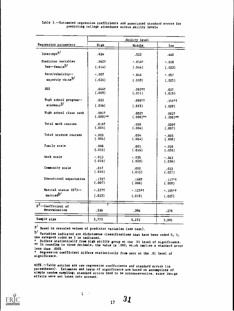
Table 3.--Estimated regression coefficients and associated standard errors forpredicting college attendance within ability levels
Ability level
Regression parameters High Middle Low
Intercept-a/
.634 .522 .440
Predictor variables .042t -.014* -.018
Sex--female-b/
(.014) (.014) (.023)
Race/ethnicity-- -.007 -.046 -.057
majority white-b/
(.026) (.019) (.025)
SES .044t .092*t .037(.009) (.011) (.019)
High school program-- .023 .0961,t .141*t
academic-b/
(.016) (.015) (.029)
High school class rank .001t .002t .002t(.000)** (.000)** (.300)**
Total math courses .016t .009 .020t(.004) (.004) (.007)
Total science courses -.005 .004 -.003(.004) (.004) (.008)
Family scale .006 .001 -.039(.015) (.0i6) (.026)
Work scale -.013 -.035 -.043(.016) (.020) (.036)
Community scale .017 .000 .033
(.014) (.015) (.027)
Educational expectation .172t .168t .117*t(.007) (.006) (.009)
Marital status 1973-- -.227t -.125*t -.105*t
married-b/
(.023) (.018) (.025)
R2--Coefficient of
I
determination .336 .396 .276
Sample size 3,773 6,272 3,981
'1/ Based on rescaled values of predictor variables (see text).
12/ Variables indicated are dichotomous classifications that have been coded 0, 1;the category coded as 1 is indicated.* Differs statistically from high ability group at the 01 level of significance.** In rounding to three decimals, the value is .000, wh,ch implies a standard errorless than .0005.t Regression coefficient differs statistically from zero at the .01 level ofsignificance.
NOTE.- -Table entries are raw regression coefficients and standard errors (inparentheses). Estimates and tests of significance are based on assumptions ofsimple random sampling; standard errors tend to be nonconservative, since designeffects were not taken into account.
17
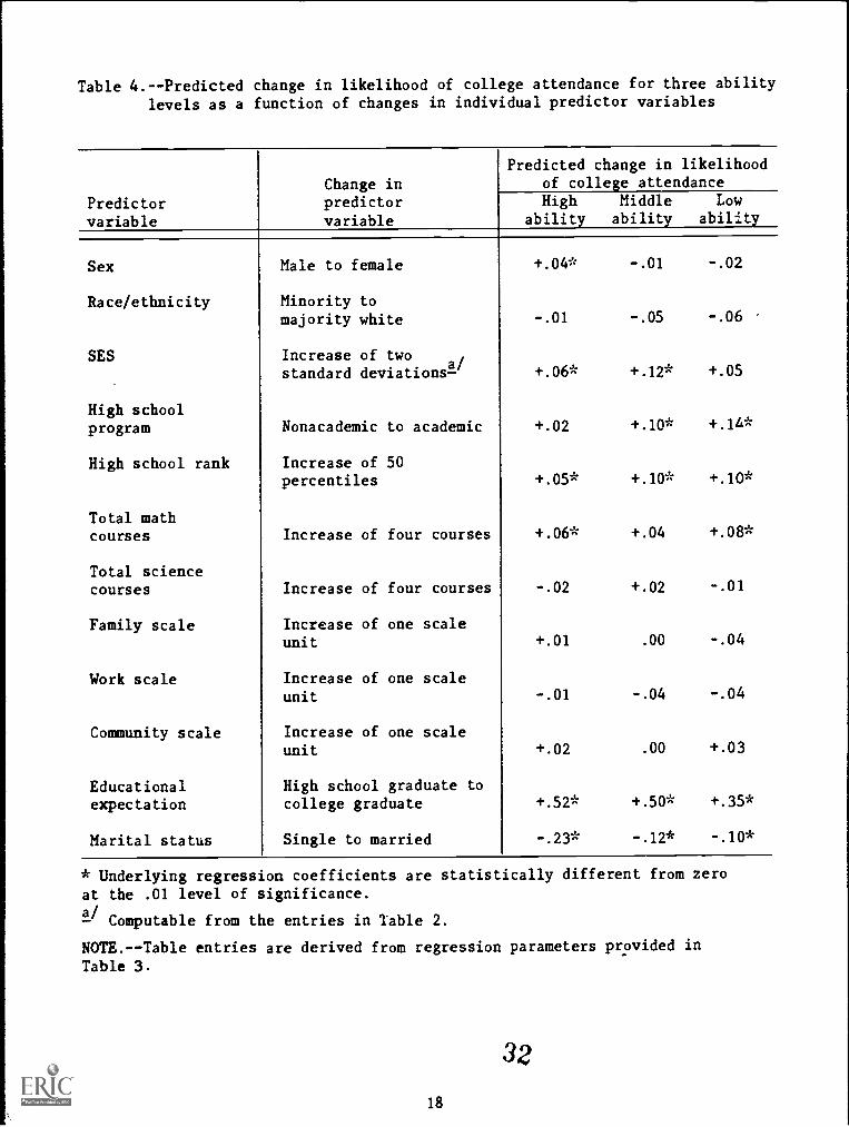
Table 4.--Predicted change in likelihood of college attendance for three abilitylevels as a function of changes in individual predictor variables
Predictorvariable
Change inpredictorvariable
Predicted change in likelihoodof college attendanceHigh
abilityMiddleability
Lowability
Sex Male to female +.04* -.01 -.02
Race/ethnicity Minority tomajority white -.01 -.05 -.06
SES Increase of twostandard deviations!
/+.06* +.12* +.05
High schoolprogram Nonacademic to academic +.02 +.10* +.1A*
High school rank Increase of 50percentiles +.05* +.10* +.10*
Total mathcourses Increase of four courses +.06* +.04 +.08*
Total sciencecourses Increase of four courses -.02 +.02 -.01
Family scale Increase of one scaleunit +.01 .00 -.04
Work scale Increase of one scaleunit -.01 -.04 -.04
Community scale Increase of one scaleunit +.02 .00 +.03
Educational High school graduate toexpectation college graduate +.52* +.50* +.35*
Marital status Single to married -.23* -.12* -.10*
* Underlying regression coefficients are statistically different from zeroat the .01 level of significance.a/
Computable from the entries in Table 2.
NOTE.--Table entries are derived from regression parameters provided inTable 3.
32
18
These standardized coefficients are presented in Appendix A (final column of
Tables A.4, A.5, and A.6).
Although the relative importance .1f predictors generally varies with
ability level, the most predictive variable in the full regression model
remains educational expectation, within each level. The only other predictors
that are among the five most predictive for each level are marital status and
high school rank. While the overall prediction of college attendance is
significant for each ability level, it can be seen from Table 3 that not all
of the individual regression coefficients differ significantly from 0 (signif-
icant coefficients are indicated by a dagger, t). While not strictly appro-
priate, ignoring such nonsignificant coefficients facilitates interpretation14/of results, particularly differences among the ability levels.-- Also, while
an overall test for homogeneity of regression was not conducted, pairwise
tests for significance of regression coefficient differences between the high
ability group and other levels were performed. Significant differences are
indicated in Table 3 by an asterisk (*).
The intercept terms, representing the means of the base group (see
above), reflect differences in the likelihood of college attendance as a
function of ability when the remaining factors are held at constant values.
15/Although standard errors are not reported for the intercept terms,-- the
increase in the intercept with increasing ability is fairly intuitive.
14/It should be recognized that the inability to reject nullity of a value is
not equivalent to the establishment of true nullity and that the individualnullity of each of several regression coefficients is not equivalent to thenullity of the several variables considered simultaneously. Moreover, if theassumption of nullity of the nonsignificant coefficients were accepted as aconstraint of the regression model, then the regression coefficients of theremaining terms would more than likely differ somewhat from the values givenin Table 3.15/
The post hoc rescaling of the predictor variables allows simple compu-tation of the intercept that would be obtained using the resealed values;however, computation of the exact standard error of the intercept involvescomplex expressions of the variance-covariance matrix. Since the rescalingclosely approximated a centering of all variables to a mean of zero, a non-conservative estimate of the standard error of the intercept is given by
js2(1-R
2)/n, where s
2is the variance of the criterion variable (comput-
able from the entries of Table 1), and R2 is the coefficient of determination(Table 3).
19
33
Among the background variables (sex, race/ethnicity, and socioeconomic
status), none shows consistent unique prediction of college attendance at all
ability levels; in fact, race/ethnicity is not predictive at any ability
level. Increasing SES predicts an increase in college attendance for the high
and middle ability levels, more so at the latter level; for those of low
ability, SES is not a statistically significant predictor, even though the
direction and magnitude of prediction is quite similar to that for the high
ability level. Sex is a significant predictor only for high ability students,
indicating a predicted increase in attendance for females.
Among the set of variables related to academic credentials, only number
of science courses fails to predict college attendance for any ability level.
High school rank, on the other hand, shows a consistent prediction of in-
creased college attendance for all ability levels. The remaining academic
credential variables are predictive in only two ability levels. Number of
math courses consistently predicts increased attendance for the high and low
ability students; being in an academic high school program is also associated
with increased attendance for middle and low ability students.
Of the three life values variables considered, none predicts college
attendance uniquely, but both educational expectation and marital status
predict attendance at all ability levels. Not surprisingly, higher expec-
tations are associated with increased attendance; however, the predicted
attendance increase for a given increase in expectations is not as great for
low ability students as for other ability levels. Early marriage depresses
the likelihood of college attendance at all ability levels, but the effect
among high ability students is approximately double that for other ability
levels.
2. Discussion
There are obvious similarities among ability levels in the unique
relationships of the predictor variables to college attendance (i.e., no
directionally inconsistent relationships; five consistently nonpredictive
vaiables [race/ethnicity, number of science courses, and the three life
values scales]; and one consistently predictive variable, high school rank).
Nonetheless, the regression solutions are sufficiently different within the
three ability groups to suggest differential effects of some predictor varia-
bles within the high abi.iity group.16/
16/No direct test for homogeneity of regression was performed, however.
20
34
There are a large number of plausible explanations for the regression
solutions and differences, not the least of which involve limitations of the
data and/or the particular regression model. There is little doubt that some
important personal determinants of college attendance (e.g., motivational
factors) are either not included in the set of variables considered or not
adequately reflected in the particular measures employed (e.g., the life value
variables, in particular). Further, the conceptual model and the regression
model adopted do not account for interactive effects of the variables; some
such interactions might be expected on an intuitive level or as a result of
prior research. As an example, interactive effects on college attendance by
sex, race/ethnicity, and SES are likely; also, interactive effects by high
school program and number (as well as type) of math and science courses taken
may be reasonably postulated. Finally, individual characteristics cannot be
considered as the only determinants of college attendance. Characteristics of
the institution(s) to which application is made (particularly selection cri-
teria) and the nature of high school counseling programs are also potential
determinants. There is certainly no reason to expect invariance of the re-
gression parameters for the variables considered if additional variables
(either individual or contextual) and/or interactions were included in the
regression model. Despite obvious limitations of interpretation, some of the
differential effects across ability levels do lend themselves to rational (al-
though not uniquely rational) explanation.
The greater likelihood of women attending college within the highly able
group, controlling for differences in other variables, is not paralleled at
other ability levels. Although this may reflect the fact that highly able
women are more aware of the changing role of women in society, or more able to
exercise options leading to careers demanding higher education, it is consid-
ered more likely that this effect results from higher motivation among highly
able women (possibly as a result of formal or informal school or home coun-
seling) and/or of increased recruiting/selecting of highly able women by
institutions of postsecondary education. The potential for interactions among
sex, race/ethnicity, and SES also exists. An alternate hypothesis of some
depress4ng effect on high ability men is possible, but considered unlikely.
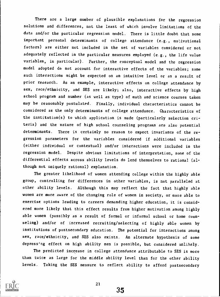
The predicted increase in college attendance attributable to SES is more
than twice as large for the middle ability level than for the other ability
levels. Taking the SES measure to reflect ability to afford postsecondary
21
35
education and also social class expectations, the differential prediction may
be related to the overall likelihood of attendance across the ability groups
(78, 46, and 21 percent, from high to low). Under these conditions it would
be reasonable for SES factors to come into play to a greater extent for the
middle ability students than for the high ability students (who likely receive
encouragement to apply to college and have greater likelihood of acceptance
because of their ability) or the low ability group (who may be discouraged
from applying to college and have lower likelihood of admission).
The increase in likelihood of college attendance attributable to an
academic high school background is inversely related to ability, greatest in
the low ability group and least in the high ability group. The high school
program in which an individual is placed is more than likely a joint function
of the individual's motivation for college and high school counseling prac-
tices. Thus, those who plan for college (with or without the help of coun-
selors) will probably be placed in an academic program. The actual incidence
of academic program background is also strongly related to ability. Two
factors may subsequently explain the differential prediction. First, low
ability students (and to a lesser extent middle ability students) may be
initially placed er subsequently transferred to a nonacademic program, with an
attendant lowering of motivation for college, at higher rates than low ability
students. Second, higher ability students may be encouraged more toward
application and accepted at higher rates than lower ability students, regard-
less of their high school curricular program.
Educational expectation is the most powerful predictor of college atten-
dance within all ability levels, but prediction is greater for high and middle
ability students. One of the most plausible explanations for such a differ-
ence is the potential for less realistic expectations within the low ability
group, in which only about one in five of the individuals had attended col-
lege.
While early marriage reduces the likelihood of attending college by more
than ten percentage points in both the low and middle ability groups, the
effect is approximately doubled for the high ability group. While it is
understandable that the additional responsibilities of marriage would depress
college-going rate, a rational explanation for the greater reduction in the
high ability group is elusive. One possible explanation for the magnitude of
differential prediction is an artifact related to the low base rate of early
3622
marriage (less than 9 percent) in the high ability group, with an associated
low variability of the marital status variable. Indeed, the discrepancies of
standardized regression coefficients (which account for differing variability
of the predictor variables) among the ability groups are less pronounced
though still directionally consistent (see Tables A.4 through A.6).
E. Modeling College Attendance
The multiple regression approach employed in the previous subsection pro-
vides an assessment of the simultaneous direct unique relationship of the pre-
dictor variables to the outcome of college attendance. Because of the nature
and extent of the covariation among the predictor variables, such relation-
ships may be expected to differ somewhat from the simple bivariate relation-
ships suggested in the results of Section II.0 and provided explicitly in the
zero order correlation coefficients (see Appendix A, Tables A.1 through A.3).
In general, the two sets of relationships are similar, but some notable excep-
tions exist. For example, the descriptive results suggest an overall advan-
tage in college attendance for high ability males over high ability females;
however, when compensating for other male-female differences in the high
ability group, the direct relationship indicates an advantage for females.
Such apparent incongruities can be investigated within a structural
model, which allows a more comprehensive examination of predictor-criterion
relationships. An additional investigation of the data was therefore under-
taken employing path analysis as applied to the model previously presented as17/
Figure 1.-- The posited model of college attendance specifies directional
relationships formulated on the basis of prior knowledge and theoretical18
considerations.--/
Given the model, the path analytic solution decomposes the
overall directional relationship of one variable to another into (1) an
indirect effect, which operates through intervening variables in the model,
and (2) a direct effect, which is unique and typically corresponds to the
direct relationship between the two variables as determined through a multiple
regression solution. To allow comparison with the zero order correlation
17/This is one of several structual equation analytic approaches; see, for
example, Kerlinger and Pedhazur (1973) or Duncan (1975).18/
Since path analytic results are model-dependent, the specification of themodel is of obvious importance.
23 37
coefficients (Tables A.1 through A.3), the analysis was conducted using stan-
dardized variables.
The path analytic solutions for the three ability level groups are pre-
sented in Appendix A (Tables A.4 through A.6). The solution for the high
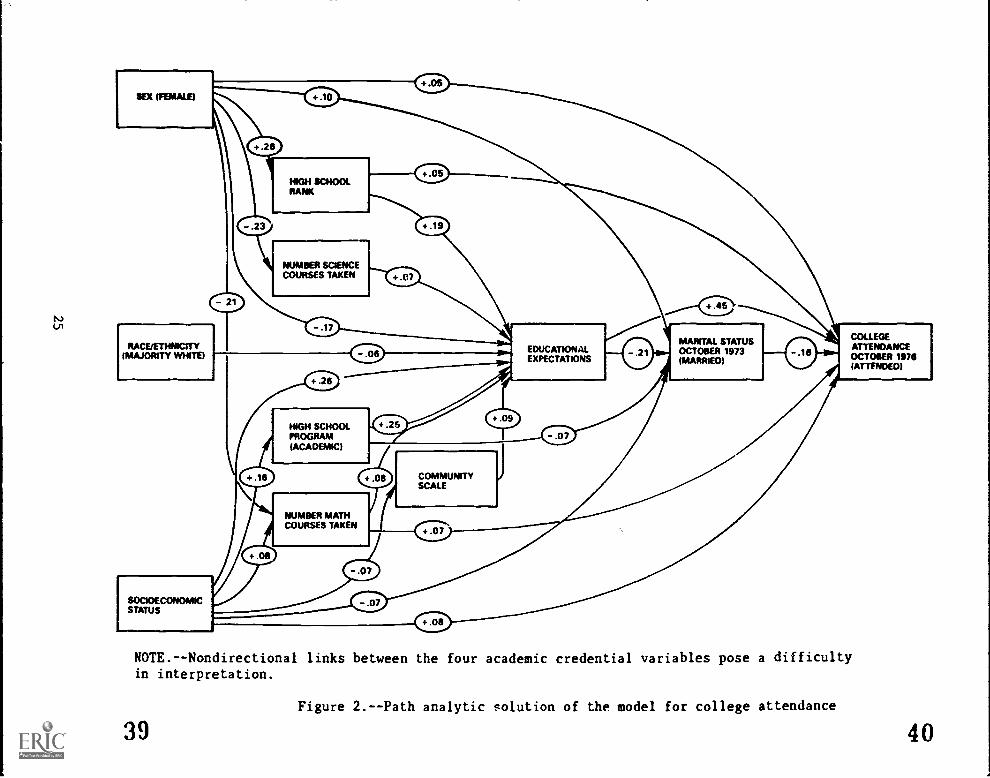
ability group is presented graphically in Figure 2. The figure expresses the
model by means of directional paths interrelating the set of variables corsid-
ered; the only paths presented are those which are associated with statis-
tically significant relationships and which ultimately link (directly or
indirectly) with the criterion variable, college attendance. A path coeffi-
cient is associated with each path shown; these are standardized coefficients
obtained in the various steps of the solution, (see Table A.6). The coeffi-
cient associated with the path leading directly from a variable of interest to
the criterion variable represents the direct effect (analogous to the multiple
regression coefficients given in the previous section, but in standardized
form); the sum of the products of coefficients associated with paths linking19
through intervening variables may be taken as the indirect effect.--/
For
example, the direct effect of educational expectations on college attendance
is .45 and the indirect effect is .03 (i.e., (-.21)(-.16)).
Perhaps the most salient aspect of Figure 2 is the major role played by
educational expectations not only in direct prediction but also in chanelling
the indirect effects of antecedent variables to the criterion variable. For
example, while high school academic program shows no direct relationship to
college attendance, the indirect effect is estimated at about .12, closely
approximating the overall effect of .19 indicated in the zero order corre-
lationlation (Table A.3).-- Also, the previously identified apparent anomaly of
the relationship of sex to college attendance is well explained by indirect
19/-- Strictly speaking this simple interpretation may be somewhat misleading,primarily as a result of the inclusion of four variables in the set repre-senting academic credentials (i.e., high school rank, number of sciencecourses taken, number of math courses taken, and high school course of study).Relationships within this set have not been specified as directional andeffectively have been assummed nondirectional. Thir introduces nondirectionallinks through which indirect effects can opelJte, and the potential operationof indirect effects through such nondirectional links provides an interpreta-tional difficulty.20/-- Nondirectional links between the four academic credential variables posesome problems in interpretation.
2.4
38
SEX
+.26
HIGH SCHOOLRANK
- .23
NUMBER SCIENCECOURSES TAKEN
RACE/ETHNICITY(MAJORITY WHITE)
- 21 .............--.45
SOCIOECONOMICSTATUS
EDUCATIONALEXPECTATIONS
MARITAL STATUSOCTOBER 1973(MARRIED)
HIGH SCHOOLPROGRAM(ACADEMIC)
+ .09
COMMUNITYSCALE
NUMBER MATHCOURSES TAKEN
.07
COLLEGEATTENDANCEOCTOBER 1976(ATTENDED)
NOTE.--Nondirectional links between the four academic credential variables pose a difficultyin interpretation.
Figure 2.--Path analytic solution of the model for college attendance
39 40
effects through expectations. While the direct effect of sex is +.05 (indi-
cating an advantage to females), the indirect effects through early marriage
(-.02) and those chanelled through expectation (-.07) offset the direct effect21
to an overall negative relationship (indicating an advantage to males).--/
The role played by educational expectation also points to a potential
misspecification of the model (or more precisely to the omission of an impor-
tant variable). While the measure of educational expectation was taken during
the senior year in high school (at a point in time following most of the
school activities contributing to the academic credential variables), it is
anticipated that these expectations reflect to a large degree previous expec-
tations (which could antedate the academic credential variables). To the
extent that that this is true, educational expectation is perhaps misplaced in
the directional flow of the model.
A comparison of the path analytic solution for high ability students with
those of other ability levels can be made by reference to Tables A.4 through
A.6. Direct effect differences have been discussed in the previous section;
however, some indirect differences also exist. Nonetheless, the patterns of
relationships among the ability level groups show considerably greater simi-
larity than difference.
21/-- Indirect effects operating through the academic credential variables thatare not chanelled through expectations are effectively zero.
26 41
III. ACTIVITIES IN 1976
A second series of analyses examined the current activities of individ-
uals as a function of college attendance and ability level, to compare life
outcomes for the talent loss group to those of other ability levels who did
not attend college and to suggest potential effects of nonattendance among
highly able (and other ability level) students. The constructs considered in
these analyses were those considered of major importance in subsequent life
objectives and addressable from available NLS data: family formation, job
attainment, and job satisfaction. These topics are treated separately in the
following subsections.
Results are provided for both the college and noncollegc groups; however,
it should be recognized that the results apply to a point in time that is
still relatively early in the adult life of the high school class of 1972 and
that neither occupational nor family patterns can be assumed to have stablized
for some groups (particularly among those who attended college). Moreover,
insufficient time had elapsed since high school graduation to allow individ-
uals to attain entry to professional careers requiring considerable postsec-
ondary training. Consequently, the more meaningful comparisons for most of
these analyses are those between ability levels within the noncollege group.
A. Family Formation
Table 5 presents three indices of family formation for the college and
noncollege groups within each ability level: (1) percent who had been married
by October 1976, (2) percent who were parents by October 1976, and (3) the
ratio of (2) to (1), which reflects the conditional parenthood rate among
those married0 Those in the talent loss group were somewhat less likely to
have married by October 1976 than those in noncullege groups at other ability
levels (although the difference is marginally nonsignificant in comparing to
the low ability level). Also, as might be expected, highly able people who
did not attend college were twice as likely as their college-attending coun-
terparts to have married within four and one-half years after high school.
22/Interpretation of the ratio as a conditional rate is not strictly appro-
priate, since it does. not account for unmarried parents.
27 4 2
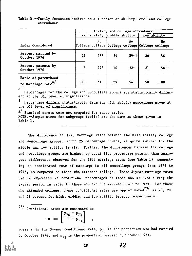
Table S.--Family formation indices as a function of ability level and collegeattendance
Index considered
Ability and college attendanceHigh ability Middle ability Low ability
NoCollege college
No
College collegeNo
College college
Percent married byOctober 1976
26 53* 34 59*t 36 58
Percent parents byOctober 1976
5 27* 10 32* 21 58*t
Ratio of parenthooda/
to marriage rate.19 .51 .29 .54 .58 1.00
Percentages for the college and noncollege groups are statistically differ-ent at the .01 level of significance.
Percentage differs statistically from the high ability noncollege group atthe .01 level of significance./
Standard errors were not computed for these ratios.NOTE.--Sample sizes for subgroups (cells) are the same as those given inTable 1.
The difference in 1976 marriage rates between the high ability college
and noncollege groups, about 25 percentage points, is quite similar for the
middle and low ability levels. Further, the differences between the college
and noncollege groups are higher, by about five percentage points, than analo-
gous differences observed for the 1973 marriage rates (see Table 1), suggest-
ing an accelerated rate of marriage in all noncollege groups from 1973 to
1976, as compared to those who attended college. These 3-year marriage rates
can be expressed as conditional percentages of those who married during the
3-year period in ratio to those who had not married prior to 1973. For those23
who attended college, these conditional rates are approximated--/
as 23, 29,
and 26 percent for high, middle, and low ability levels, respectively.
23/Conditional rates are estimated as
[P76 P73]r = 100 1 - p73
where r is the 3-year conditional rate, p76 is the proportion who had married
by October 1976, and p73 is the proportion married by October 1973.
28 43
Comparable conditional rates for those who did not attend college are about
twice as great (46, 51, and 40 percent). Differences in the 3-year marriage
rate between the college attendance groups are markedly greater than those
among ability levels within a college attendance category.
Differences in the incidence of parenthood are also indicated in Table 5.
Parenthood rates vary much more dramatically than marriage rates over ability
levels. Those in the talent loss group are much less likely (by a factor of
one-half) to have become parents by October 1976 than the low ability noncol-
lege group, and slightly less likely than the middle ability group. Even
among those who attended college the parenthood rate increases with decreasing
ability; however, those who did not attend college are much more likely to
have one or more children by 1976 than those who attended, regardless of
ability level.
Since parenthood r2tes are typically confounded with marriage rates,
conditional parenthood probabilities (ratios of parenthood rate to marriage
rate) were computed to facilitate interpretation. The conditional parenthood
probabilities shown in Table 5 decrease monotonically with increasing ability,
for both the college and noncollege groups; and, within each ability level,
are approximately *mice as large for those in the noncollege group. While the
conditional parenthood probabilities for the high ability level are less than
those for other ability levels, they do not differ greatly from those of the
middle ability level. Probabilities for both of these levels, however, differ
dramatically from those for low ability, which are approximately twice as
great for both those who attended college and those who did not.
While the 1976 family formation indices reflect to some extent the early
marriage (1973) rates presented previously (Table 1), they clearly point out a
strong relationship between college attendance and family formation. There
are, of course, real difficulties in combining the pursuit of higher education
with support of a family, and an explicit or implicit choice between one or
another of these alternatives quite likely underlies the findings of differ-
ences between college goers and nongoers at all ability levels. Differences
among ability levels probably reflect well-established relationships between
SES and ability on the Ole hand and SES and marriage patterns on the other,
but also may indicate that a more conscious or deliberate choice is exercised
by the highly able in beginning a family or pursuing higher education.
2944
B. Job Attainment
The measures of job attainment examined were employment status, earnings,
and fulfillment of career expectations. To provide more meaningful results,
persons who were fill- or part-time students in October 1976 were excluded
from these analyses. In interpreting the results, this exclusion should be
kept in mind.
1. Employment Status
Figure 3 depicts the employment status for those who had attended
college and those who had not for each ability level; the unemployed are
further categorized cn the basis of whether they were in (looking for work) or
out (not looking for work) of the labor force. The employment status distri-
butions for the talent loss group are quite similar to those of noncollege
groups of less ability. Likewise, the distributions for those who attended
college are quite similar (the apparent differences for the low ability group
are not statistically significant); however, differences between college and
noncollege groups within the three ability levels are more pronounced.
For all ability levels, the most obvious difference in employment status
between the college and noncollege group is in the "cut of labor force" compo-
nent. High ability students who had not attended college were absented from
the labor force at twice the rate of those who had attended; this ratio of 2
to 1 (as well as the actual percentages) is quite similar for middle ability
students. Among low ability students, the difference is directionally con-
sistent and significant but the ratio is lower. The college-noncollege dif-
ferences are consonant with the findings of the previous subsection that those
in the noncollege group were more likely to have married and to have become
parents by October 1976. As such, it could be expected that more of the
noncollege group would be engaged in full-time homemaking.
Of the percentages shown in Figure 3, the relative number of individuals
who are unemployed and looking for work is consistently greater in the college
group but is significantly different (and only marginally so) only within the
high ability group; the difference in the relative numbers employed is signif-
icant only within the middle ability group. Given the differences between the
college and noncollege groups in percentages out of the labor force, however,
interpretation of these differences can be misleading. Employment rates can
be interpreted more meaningfully by excluding those who are not in the work
4530
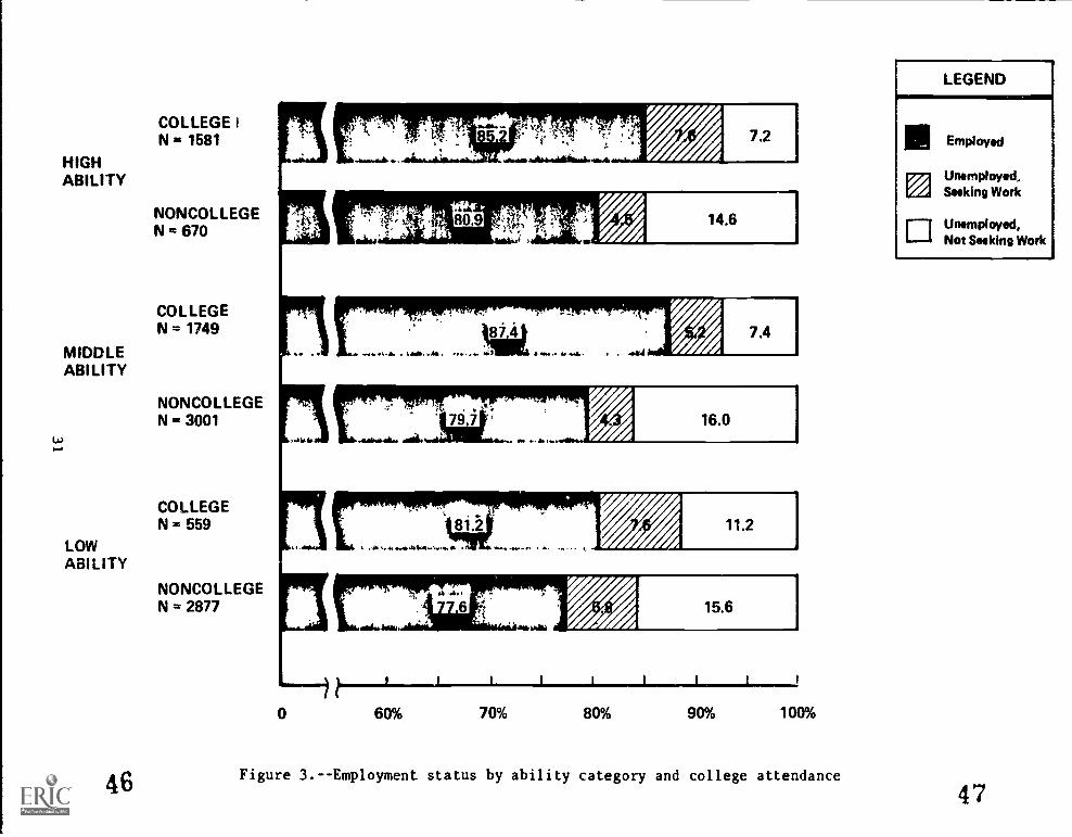
HIGHABILITY
MIDDLEABILITY
LOWABILITY
46
COLLEGE IN = 1581
NONCOLLEGEN = 670
COLLEGEN = 1749
NONCOLLEGEN = 3001
COLLEGEN = 559
NONCOLLEGEN = 2877
0 60% 70% 80% 90% 100%
Figure 3.--Employment status by ability category and college attendance
LEGEND
IIIEmployed
ra Unemployed,Seeking Work
Q UnemPloyed.Not Seeking Work
47
24/force. Such conditional rates indicate overall employment of about 93
percent (t 2 percent) in the six groups considered, suggesting no major dif-
ferences within or among ability levels.
2. Hours Worked and Earnings
For those who were employed (full-time or part-time), average hours
worked and earnings per week were computed; results are given in Table 6.
Hours worked per week averages slightly greater than 40 for all ability
levels, and does not differ markedly between college and noncollege groups.
Standard deviations for hours worked are likewise similar, suggesting no major
differences in the distributions of hours worked as a function of ability or
of college attendance. Given a fairly standard work week and the exclusion
from these analyses of those still in school, such a result is not particu-
larly surprising.
Average weekly earnings are also fairly consistent (ranging from about
$168 to $176 dollars) regardless of ability or college attendance. At first
glance, this result may seem somewhat counterintuitive; however, several
factors (including the time point considered and group definitions) could
contribute to this lack of difference. First, as mentioned previously, those
preparing for professional positions requiring longer schooling (and typically
representing higher earnings) were probably still in college. Further, those
who attended only trade or business school were included in the noncollege
group for purposes of this report. Also, those in the noncollege group were
likely to be substantially further along in their careers than those in the
college group. Those whu had completed a 4-year college program would be just
starting iu a job in October 1976, while those who began work on receipt of
their high school diploma could be about four and one-half years into a job.
Even those who had some college bqt left before completing their degrees or
those who graduated from 2-year programs would have had less time on the job
(by about a factor of one-half). Moreover, there are quite likely individuals
24/ Conditional employment rates can be obtained from the values in Figure 3
as
r = 100p/(1-1)*)]
where r is the conditional rate, p is the raw employment proportion fromFigure 3, and p* is the proportion of individuals not in the work force from
Figure 3.
32 48
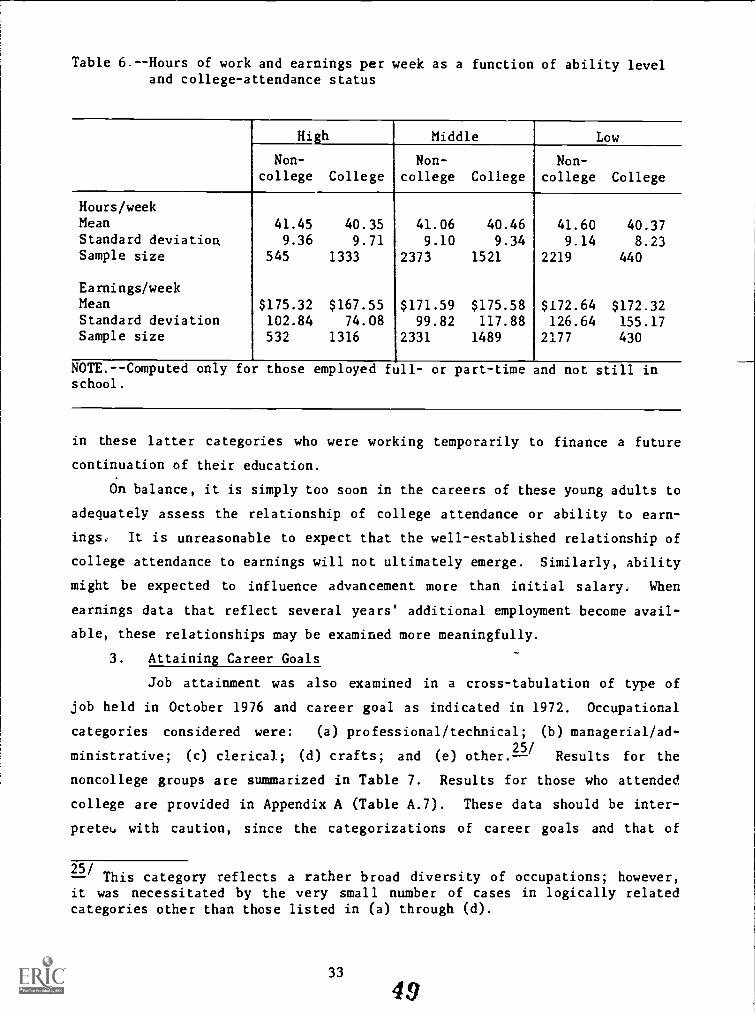
Table 6.--Hours of work and earnings per week as a function of ability leveland college-attendance status
High Middle Low
Non-college College
Non-college College
Non-college College
Hours/weekMean 41.45 40.35 41.06 40.46 41.60 40.37Standard deviation 9.36 9.71 9.10 9.34 9.14 8.23Sample size 545 1333 2373 1521 2219 440
Earnings/weekMean $175.32 $167.55 $171.59 $175.58 $172.64 $172.32Standard deviation 102.84 74.08 99.82 117.88 126.64 155.17Sample size 532 1316 2331 1489 2177 430
-- Computed only for those employed full- or part-time and not still inschool.
in these latter categories who were working temporarily to finance a future
continuation of their education.
On balance, it is simply too soon in the careers of these young adults to
adequately assess the relationship of college attendance or ability to earn-
ings. It is unreasonable to expect that the well-established relationship of
college attendance to earnings will not ultimately emerge. Similarly, ability
might be expected to influence advancement more than initial salary. When
earnings data that reflect several years' additional employment become avail-
able, these relationships may be examined more meaningfully.
3. Attaining Career Goals
Job attainment was also examined in a cross-tabulation of type of
job held in October 1976 and career goal as indicated in 1972. Occupational
categories considered were: (a) professional/technical; (b) managerial/ad-25/
ministrative; (c) clerical; (d) crafts; and (e) other. Results for the
noncollege groups are summarized in Table 7. Results for those who attended
college are provided in Appendix A (Table A.7). These data should be inter-
pretet with caution, since the categorizations of career goals and that of
25/This category reflects a rather broad diversity of occupations; however,
it was necessitated by the very small number of cases in logically relatedcategories other than those listed in (a) through (d).
33
46
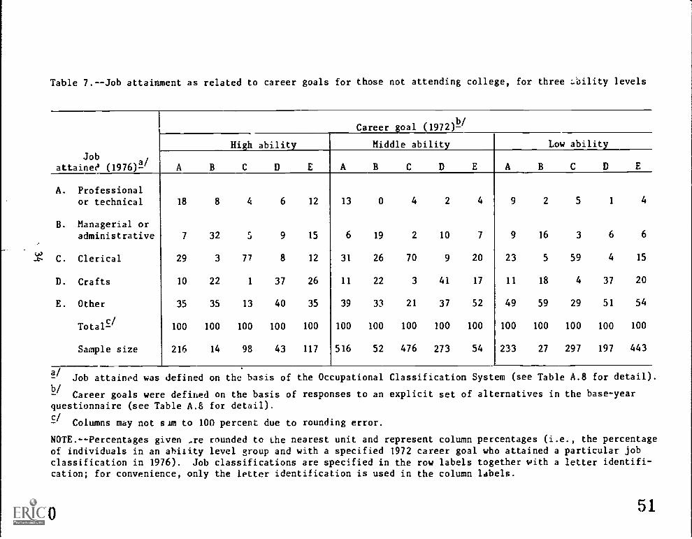
Table 7.--Job attainment as related to career goals for those not attending college, for three Lbility levels
Jobattained (1976)1
/
Career goal (1972)1
High ability Middle ability Low ability
C D E A B C D E A BC DEA. Professional
or technical 18 8 4 6 12 13 0 4 2 4 9 2 5 1 4
B. Managerial oradministrative 7 32 5 9 15 6 19 2 10 7 9 16 3 6 6
C. Clerical 29 3 77 8 12 31 26 70 9 20 23 5 59 4 15
D. Crafts 10 22 1 37 26 11 22 3 41 17 11 18 4 37 20
E. Other 35 35 13 40 35 39 33 21 37 52 49 59 29 51 54
Total.C./
100 100 100 100 100 100 100 100 100 100 100 100 100 100 100
Sample size 216 14 98 43 117 516 52 476 273 54 233 27 297 197 443
1/
Job attained was defined on the basis of the Occupational Classification System (see Table A.8 for detail).b/
Career goals were defined on the basis of responses to an explicit set of alternatives in the base-yearquestionnaire (see Table A.8 for detail)./
Columns may not sun to 100 percent due to rounding error.
NOTE.--Percentages given .re rounded to the nearest unit and represent column percentages (i.e., the percentageof individuals in an ability level group and with a specified 1972 career goal who attained a particular jobclassification in 1976). Job classifications are specified in the row labels together with a letter identifi-cation; for convenience, only the letter identification is used in the column labels.
50 51
type of job attained are differently based.26/
Moreover, because of the broad
categorization of careers, an individual who planned to become an engineer but
instead became a teacher would still fall in the same category (professional/
technical) as another who planned for and actually found work as an engineer.
Also, it is still early in the career of these individuals, and data are not
available to determine if respondents are actively planning to change jobs or
seek further training in the near future.
Even in light of these limitations, and additional limitations of small
sample sizes for some of the subgroups considered, it is fairly obvious from
Table 5 that relatively few of the noncollege group had attained the occupa-
tional goal they aspired to as seniors in high school. Excluding the "other"
category (which is in actuality only a residual classification), only among
those who aspired to clerical positions had a majority of individuals actually
realized their career goals. Although not explicit in Table 7, the talent
loss group aspired to professional/technical occupations at somewhat higher
rates (about 43 percent) than the middle ability noncollege group and at more
than twice the rate of the low ability noncollege group. Moreover, irrespec-
tive of career goal, noncollege individuals of high ability had attained
professional/technical positions at higher rates than those of lesser ability.
Among those attending college (Table A.7), much larger percentages of
individuals had aspired to professional/technical occupations within each of
the ability levels, and among those so aspiring, greater percentages (by
27factors of at least 2) had attained such positions.--
/As with the noncollege
group both aspiration for and attainment of professional/technical occupations
decrease with decreasing ability. An explicit comparision of college and
noncollege groups at the high ability level is also provided in Appendix A
(Table A.8).
26/- Respondents used an explicit set of categories to indicate career goals in1972, while job attained In 1976 was a categorization of job classificationaccording to the Occupational System used by the Bureau of the Census (seeLevirir.ohn et al., 1978, Appendix C).27/
Ignoring career goals and considering only job category attained by 1976,fully one-third of the highly able persons with prior college experience hadattained professional or skilled technical positions, while only 12 percent ofthose without college experience worked in such positions (see Table A.7).
3552
C. Job Satisfaction
Satisfaction ratings were obtained from NLS third follow-up respondents
on several facets of their job situations in October 1976. Ratings of the
three ability levels within the noncollege group are presented in Table 8.
Comparable ratings for those who attended college are given in Appendix A
(Table A.9). Individuals still in school were also excluded from these
analyses.
These results are, in general, rather sterile; for all job facets and all
ability levels, in both the college and noncollege groups the modal response
is mild satisfaction. Some differences exist in expressed satisfaction among
the various facets of current job (least satisfaction with opportunity for
promotion and greatest satisfaction with respect from others for being in the
line of work); however, the distributions of satisfaction ratings for a given
facet of the job are remarkably similar among the ability levels and between
the college and noncollege groups. College-educated individuals are more
likely than noncollege individuals to indicate the extremes of "very satis-
fied" or "very dissatisfied," but overall there is no appreciable difference
in job satisfaction between the two groups. While the lack of diversity of
response may reflect, to some extent, the relatively short time most individ-
uals have been working, it is believed that technical problems in the measure-
ment of satisfaction (e.g., response set, prepotency of categories, and halo
effect) present a more likely explanation.
5336
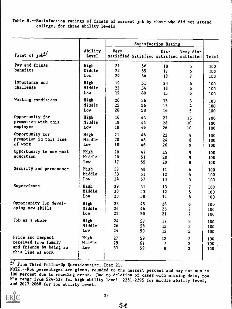
Table 8.--Satisfaction ratings of facets of current job by those who did not attendcollege, for three ability levels
a/jobFacet of obAbilityLevel
Satisfaction Rating
Very Dis- Very dis-satisfied Satisfied satisfied satisfied Total
Pay and fringe High 21 56 18 5 100benefits Middle 22 55 17 6 100
Low 20 54 19 7 100
Importance and High 19 51 23 6 100challenge Middle 22 54 18 6 100
Low 19 60 13 6 100
Working conditions High 26 56 15 3 100Middle 25 56 15 4 100Low 20 58 16 5 100
Opportunity for High 16 45 27 13 100promotion with this Middle 18 44 28 10 100employer Low 18 46 26 10 100
Opportunity for High 21 46 23 9 100promotion in this line Middle 20 48 24 8 100of work Low 18 46 26 9 100
Opportunity to use past High 20 47 25 9 100education Middle 20 51 20 9 100
Low 17 55 20 8 100
Security and permanence High 37 48 11 4 100Middle 33 51 12 4 100Low 24 57 13 5 100
Supervisors High 29 51 13 7 100Middle 30 53 12 5 100Low 23 58 12 6 100
Opportunity for devel- High 23 45 26 6 100oiling new skills Middle 24 46 23 7 100
Low 23 50 21 7 100
Job as a whole High 24 57 17 3 100Middle 26 58 13 3 100Low 24 59 12 5 100
Pride and respect High 27 59 12 2 100received from family Middle 29 61 7 2 100and friends by being inthis line of work
Low 31 59 8 2 100
! From Third Follow-Up Questionnaire, Item 21.NOTE.--Row percentages are given, rounded to the nearest percent and may not sum to100 percent due to rounding error. Due to deletion of cases with missing data, rowN's range from 524-537 for high ability level, 2261-2295 for middle ability level,and 2027-2068 for low ability level.
37
54
IV. SUMMARY AND DISCUSSION
This study has addressed two basic issues of talent loss among young
adults: (1) the determinants of college nonattendance by highly able students
and (2) some short-term consequences of nonattendance among these students as
compared to less able students who did not attend college. Of particular
concern was the determination of whether influences on and results of college
attendance were unique to highly able students or simply reflections of more
general influences applicable to those of other ability levels. In general,
otudy findings indicate that the effects on and of college attendance are
basically similar for all ability levels. Where differences exist, they are
quantitative rather than qualitative, suggesting that similar factors affect
and are affected by college attendance but that they operate and are operated
upon to a different extent for the highly able student.
A. Potential Determinants of College Attendance
Three approaches to analysis were undertaken in examining potential
determinants of college attendance: (1) descriptive comparison, indicating
univariate differences between the college and noncollege groups irrespective
of differences that exist on concomitant variables; (2) multiple regression
analysis, indicating the unique direct effects of each variable when consid-
ered simultaneously with other variables, and (3) path analysis, indicating
both the direct and indirect effects of variables, within a specified model of
college attendance. In total, these analyses present a comprehensive and
consistent set of results.
Although highly able students, as a group, entered college at a markedly
higher rate than less able students, the talent loss problem was significant;
more than one in five of those in the upper ability quartile of 1912 high
school graduates had not attended college by October 1976. The factors asso-
ciated wit% college attendance, however, were similar regardless of ability
level. Students tended to enter college in lower relative numbers if they
were of lower SES, had a less adequate high school background, and had lower
expectations for eventual educational attainment. Also, early marriage was
38 55
associated with college nonentry. Educational expectation was the most power-
ful predictor of college attendance at all ability levels; however, since
expectatioL was measured during the spring term of the senior year of high
school, it probably reflected, in at least some cases, knowledge of successful
college application and certainly reflected knowledge of nonapplication.
Among the academic credential variables, only number of high school science
courses failed to show a unique relationship to college attendance. Race/eth-
nicity and life values (as measured in this study) also were not uniquely
related to college attendance at any ability level.
Some notable differences in predicted college attendance were observed
among highly able students. When other factors were controlled, sex was
related to college attendance exclusively at the high ability level, indi-
cating that men were less likely to enter college than women. When indirect
effects were considered, however, this advantage to women was reversed.
Alternately, only among highly able students was there no direct unique rela-
tionship of an academic high school program to increased college attendance.
Considering indirect effects, however, an overall advantage in college atten-
dance to those in an academic high school program was observed for those in
the high ability group as well as for other ability levels. It is considered
likely that both of these differences were related to factors not measured in
this study; in the first case, to recently increased recruiting of highly able
women and, in the second case, to formal or informal counseling of highly able
students to attend college regardless of high school course of study.
Most of the differential unique prediction of college attendance among
ability levels was a matter of degree. Educational expectation was markedly
less predictive for low ability students, suggesting more realistic expecta-
tions for high ability students. The depressing unique effect of early mar-
riage on college attmdance was about twice as great among highly able stu-
dents than at other ability levels, possibly indicating the exercise of more
conscious or deliberate choices by those of high ability between beginning a
family or pursuing higher education. Also, the unique effect of SES on col-
lege attendance was twice as great for the middle ability group than for high
(or low)_ability students. This finding is not particularly surprising, since
one might expect SES influences (e.g., ability to fund a college education and
39 56
social class expectations) to come into play more dramatically for groups in
which college entry decisions are less predictable by ability alone.
There are several implications, suggesting further research on why highly
able students do not attend college, indicated by the findings of this study.
Clearly some high ability individuals do not expect to attend college, others
expect to attend but do not. The reasons for lack of expectation or for not
realizing expectations among the highly able deserve attention. It is likely
that the tight labor market for college graduates coupled with the high cost
of a college education may lead students -.0 believe that a college ed%cation
is not a good investment (Freeman and Holloman, 1975). There is also a strong
indication that these students see marriage and full-time student status as
incompatible. Both of these potential reasons represent areas that could be
addressed through appropriate counseling.
There are other areas suggesting a need for coordinated counseling of the
highly able high school. student. It seems likely that some of these students
do not obtain proper academic credentials for admission to the college of
their choice, which may reflect improper guidance. Educators would be well
advised to examine whether many of the able young people were wrongly advised
to enter a nonacademic track or were not adequately encouraged to take more
science and mathematics courses. Finally, the direct unique relationship
between SES and college attendance suggests that some highly able students may
not be attending college for financial reasons. Although need to work in
order to support the family is a persistent inhibitor of continued education,
the actual financing of education is facilitated by several programs for needy
students. Effective counseling should ensure that the able student is fully
aware of the many financial options that exist.
B. Consequences of College Nonattendance
The examination of the consequences of college nonattendance was less
revealing, probably due to the relatively early period in the adult life of
these young people (i.e., four and one-half years after high school gradua-
tion) at which the outcomes were measured. The few observed differences in
life outcome typically were more strongly related to college attendance than
to ability level.
Some rather intuitive relationships existed between college attendance
and family formation. Highly able students who did not attend college had
40
married at about twice the rate of their cohorts who attended college, a
relationship quite similar to that for other ability levels. Similarly,
parenthood rates were considerably greater in the noncollege group at all
ability levels, and such rates were inversely related to ability regardless of
college attendance.
Highly able students who did not attend college tended to define them-
selves out of the work force at greater rates than the college-going group
(but at similar rates to those of less ability who did not attend college), a
factor probably related to higher marriage rates in the noncollege group and
thus relatively more individuals describing themselves as full-time home-
makers. Considering only those in the work force, however, employment rates
did not differentiate the college and noncollege groups or the various ability
levels. The highly able students who had not attended college generally were
more likely than noncollege groups of lower ability to have aspired to and
attained professional or technical positions. Also, a larger proportion of
those with college experience were employed in professional or technical
positions. Other occupational outcomes (job satisfaction, attaining career
goals, hours worked, earnings) suggested few marked or systematic differences
between college and noncollege groups or among ability levels.
The findings regarding occupational outcomes obviously are restricted by
temporal factors. Those who did not attend college potentially had a much
greater time in the work force than the college-going group (those who com-
pleted a nonaccelerated 4-year college program would have been in the work
force only about half a year at the time of data collection). Additionally,
those still in college were excluded from analyses. While this provides a
more meaningful analysis, it also introduces a clear bias into the findings.
Those who were pursuing an occupation requirinc professional or graduate
school attendance (typically representing higher paid occupations) were quite
likely still in school and were not represented in the findings. Allowing
additional time for entry of these individuals into the work force, and for
advancement among those. who had entered at the time of this study, should
provide for results that more closely reflect the established advantages of a
college education and that are more likely to tap effects of ability in the
occupational setting.
41
58
REFERENCES
Astin, A. W. Who goes where to college? Chicago: Science Research Asso-
ciates, 1965.
Bailey, J. P., Jr., and Collins, E. Entry into postsecondary education.
Paper presented at the annual meeting of the American EducationalResearch Association, New York, 1977.
Bowers, W. J., Pierce, G. L., Blitch, C., and Carr, A. A 'cess to post-
secondary education. Boston, Mass.: Russell B. Stearns Center for
Applied Social Research, Northeastern University, 1977.
College Entrance Examination Board. Equality of educational opportunity:
Effects of poverty and minority status. New York: College Entrance
Examination Board, 1974.
Duncan, O. D. Introduction to structural equation models. New York:
Academic Press, 1975.
Dunteman, G. H., Peng, S. S., and Holt, M. M. National Longitudinal Study
of the High School Class of 1972: Composite score analyses--ability
index, SES index, some psychological and educational construct scales.Research Triangle Park, N.C.: Research Triangle Institute, 1974.
Freeman, P., and Hollomon, J. H. The declining value of college going.
Change, 1975, 7 (7), 24-31, 52.
Kerlinger, F. N., and Pedhazur, E. J. Multiple regression in behavioral
research. New York: Holt, Rinehart & Winston, 1973.
Kish, L. Confidence intervals for clustered samples. American Socio-
logical Review, 1957, 22, 154-165.
Kish, L., and Frankel, M. R. Balanced repeated replication for standard
errors. Journal of the American Statistical Association, 1970, 65,1071-1094.
Levinsohn, J. R., Henderson, L. B., Riccobono, J. A., and Moore, R. P.National Longitudinal Study: Base year, first, second, and third
follow-up data file users manual. Research Triangle Park, N.C.:
Research Triangle Institute, 1978.
National Center for Education Statistics. Withdrawal from institutions of
higher education. Washington, D.C.: U.S. Government Printing Office,
1977 (Report #NCES-77-264).
Peng, S. S. Trends in the entry to higher_education: 1961-1972.
Educational Researcher, 1977, 6 (1), 15-19.
Peng, S. S., Bailey, J. P., Jr., and Eckland, B. K. Access to higher
education: Results from the National Longitudinal Study of the High
School Class of 1972. Educational Researcher, 1977, 6 (11), 3-7.
43
59
REFERENCES(continued)
Peng, S. S., and Jaffe, J. A. Women who enter male-dominated fields of studyin higher education. Research Triangle Park, N.C.: Research TriangleInstitute, 1978.
Thomas, G. E., Alexander, K. L., and Eckland, B. K. Access to highereducation: How important are sex, social class and academic creden-tials for college access? Baltimore, Maryland: The Johns HopkinsUniversity, 1977.
60
44
Appendix A
Supplementary Tables
61
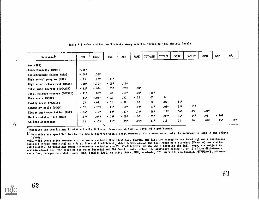
2,
Table A.1.--Correlation coefficients among selected variables (low ability level)
Variable!/
SEX RACE I SES HSP RANK I TOTMATH TOTSCI WORK FAMILY COMM EXP
Sex (SEX)
Race /ethnicity (RACE) -.06*
Socioeconomic status (SES) -.06* .36*
High school program (HSP) -.03 -.10* .11*
High school class rank (RANK) .20* -.10* -.05* .15*
Total math courses (TOTMATH) -.12* -.08* .05* .20* .08*
Total science courses (TOTSCI) -.11* -.05* .02 .19* .06* .45*
Work scale (WORK) -.14* -.08* -.02 .03 -.02 .03 .03
Family scale (FAMILY) .03 -.01 -.02 -.01 .03 -.02 -.03 .14*
Community scale (COMM) -.02 -.23* -.11* .10* .07* .07* .08* .27* .13*
Educational expectation (EXP) -.04* -.19* .12* .27* .19* .18* .14* .06* .03 .21*
Marital status 1973 (M73) .17* .04* -.08* -.09* -.00 -.09* -.05* -.04* .04* .03 -.16*
College attendance .01 -.13* .11* .25* .20* .17* .11 .01 .00 .09* .45*
N
I M73
-.16*
Indicates the coefficient is statistically different from zero at the .01 level of significance.
Variables are specified in the row labels together with a short mnemonic; for convenience, only the mnemonic is used in the column
labels.NOTE.--The correlation between a dichotomous variable (the first two, fourth, and last two listed in row labeling) and a continuous
variable (those remaining) is a Point Biserial Coefficient, which canr3t assume the full range of a standard (Pearson) correlation
coefficient. Correlations among dichotomous variables are Phi Coefficients, which, while assuming the full range, are subject to
certain anomalies. The signs of all Point Biserial and Phi Coefficients reflect the arbitrary coding (0 or 1) of the dichotomous
variables; categories coded 1 are: SEX, female; RACE, majority white; HSP, academic; M73, married; and COLLEGE ATTENDANCE, attended.
62
63
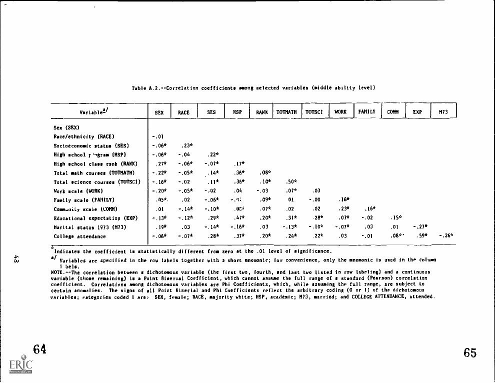
Table A.2.--Correlation coefficients among selected variables (middle ability level)
a/Variable- SEX RACE SES I HSP I RANK
.17*
.36* .08*
.36* .10*
.04 -.03
-.W. .09*
.0C1 .07*
.47* .20*
-.16* .03
.37* .20*
TOTHATH
.50*
.07*
01
.02
.31*
-.13*
.24*
TOTSCI
.03
-.00
.02
.28*
-.10*
.22*
WORK
.16*
.23*
.07*
-.07*
.03
I FAMILY I COMM
.15*
.01
.08**
EXP
-.27*
.59*
M73
-.26*
Sex (SEX)
Race/ethnicity (RACE)
Socioeconomic status (SES)
High school ultras (HSP)
High school class rank (RANK)
Total math courses (TOTMATII)
Total science courses (TOTSCI)
Work scale (WORK)
Family scale (FAMILY)
Comm.aiLy scale (COMM)
Educational expectation (EXP)
Marital status 1973 (M73)
College attendance
-.01
-.06*
-.06*
.27*
-,22*
-.16*
-.20*
.05*.
.01
-.13*
.19*
-.06*
.23*
-.04
-.06*
-.05*
-.02
-.05*
.02
-.14*
-.12*
.03
-.07*
.22*
-.07*
.14*
.11*
-.02
-.06*
-.10*
.29*
-.14*
.28*
.16*
-.02
.03
-.01
*Indicates the coefficient is statistically different from zero at the .01 level of significance.
a/Ou Variables are specified in the row labels together with a short mnemonic; for convenience, only the mnemonic is used in the column
I belsNOTE.--The correlation between a dichotomous variable (the first two, fourth, and last two listed in row labeling) and a continuousvariable (those remaining) is a Point Bisertal Coefficient, which cannot assume the full range of a standard (Pearson) correlationcoefficient. Correlations among dichotomous variables are Phi Coefficients, which, while assuming the full range, are subject tocertain anomalies. The signs of all Point Biserial and Phi Coefficients reflect the arbitrary coding (0 or I) of the dichotomous
variables; categories coded 1 are: SEX, female; RACE, majority white; HSP, academic; M73, married; and COLLEGE ATTENDANCE, attended.
64 65
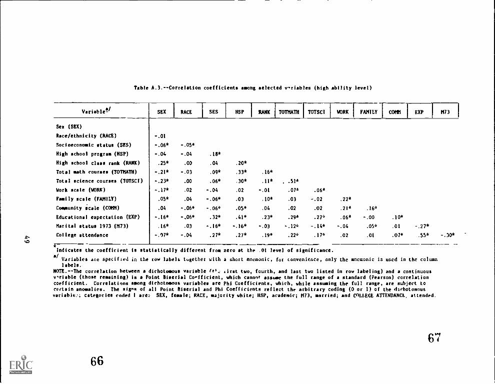
Table A.3.--Correlation coefficients among selected v-riables (high ability level)
a/Variable- SEX RACE SES HSP RANK TOTHATH TOTSCI WORK FAMILY COMM EXP I M73 I
Sex (SEX)
Race/ethnicity (RACE)
Socioeconomic status (SES)
High school program (HSP)
High school class rank (RANK)
Total math courses (TOTMATH)
Total science courses (TOTSCI)
Work scale (WORK)
Family scale (FAMILY)
Community scale (COMM)
Educational expectation (EXP)
Marital status 1973 (M73)
College attendance
-.01
-.06*
-.04
.25*
-.21*
-.23*
-.17*
.05*
.04
-.16*
.16*
-.17*
-.05*
-.04
.00
-.03
.00
.02
.04
-.06*
-,06*
.03
-.04
.18*
.04
.09*
.06*
-.04
-.06*
-.06*
.32*
-.16*
.27*
.20*
.33*
.30*
.02
.03
.05*
.41*
-.16*
.27*
.16*
.11*
-.01
.10*
.04
.23*
-.03
.19*
. .51*
.07*
.03
.02
.29*
-.12*
.22*
.06*
-.02
.02
.27*
-.14*
.17*
.22*
.21* .16*
.06* -.00 .10*
-.04 .05* .01 -.27*
.02 .01 .07* .55* -.30*
Indicates the coefficient is statistically different from zero at the .01 level of significance.a/
Variables are specified in the row labels together with a short mnemonic, for convenience, only the mnemonic is used in the columnlabels.
NOTE.--The correlation between a dichotomous variable .: drat two, fourth, and last two listed in row labeling) and a continuousvariable (those remaining) is a Point Biserial Coefficient, which cannot assume the full range of a standard (Pearson) correlationcoefficient. Correlations among dichotomous variables are Phi Coefficients, which, while assuming the full range, are subject tocertain anomalies. The signs of all Point Biserial and Phi Coefficients reflect the arbitrary coding (0 or I) of the dichotomousvariable.1; categories coded I are: SEX, female; RACE, majority white; HSP, academic; M73, married; and COLLEGE ATTENDANCE, attended.
66
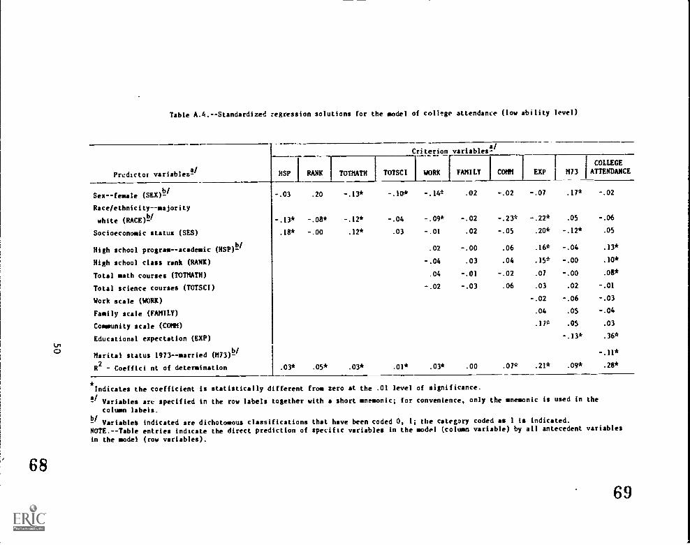
Table A.4.--Standardized regression solutions for the model of colltge attendance (low ability level)
Predictoi variablesa-/
Criteriona/
variables-
WORK FAMILY COMMi EXP H73
COLLEGE
ATTENDANCEHSP RANKI
TOTHATH TOTSCI
Sex--female (SEK)-b/
-.03 .20 -.13* -.10* -.14* .02 -.02 -.07 .17* -.02
Race/ethnicity--majority
white (RACE)-b/
-.13* -.08* -.12* -.04 -.09* -.02 -.23* -.22* .05 -.06
Socioeconomic status (SES) .18* -.00 .12* .03 -.01 .02 -.05 .20* -.12* .05
High school program--academic (HSP)-/ .02 -.00 .06 .16* -.04 .13*
High school class rank (RANK) -.04 .03 .04 .15* -.00 .10*
Total math courses (TOTHATH) .04 -.01 -.02 .07 -.00 .08*
Total science courses (TOTSCI) -.02 -.03 .06 .03 .02 -.01
Work scale (WORK) -.02 -.06 -.03
Family scale (FAMILY) .04 .05 -.04
Community scale (COMM) .17* .05 .03
Educational expectation (EXP) -.13* .36*
Marital status 1973--married (M73)-b/ -.11*
R2
- Coeffici nt of determination .03* .05* .03* .01* .03* .00 .07* .21* .09* .28*
*Indicates the coefficient is statistically different from zero at the .01 level of significance.
1/ Variables are specified in the row labels together with a short mnemonic; for convenience, only the mnemonic is used in the
column labels.b/- Variables indicated are dichotomous classifications that have been coded 0, 1; the category coded as 1 is indicated.NOTE.--Table entries indicate the direct prediction of specific variables in the model (column variable) by all antecedent variables
in the model (row variables).
69
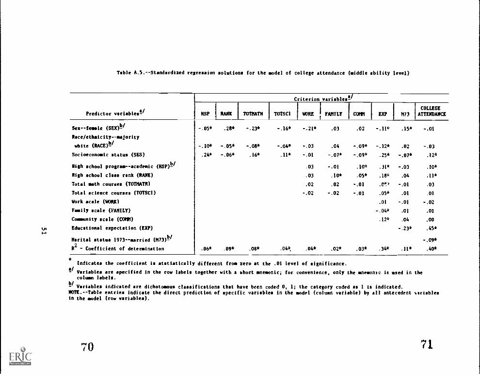
Table A.5.--Standardized repression solutions for the model of college attendance (middle ability level)
Predictor variables"-
Criterion variables"
IISP RANK TOTNATH TOTSCI WORK I FAMILYCOLLEGE
EXP I N73 I ATTENDANCE
Sex - -female (SEX)b/
Race/ethaicity--majority
white (RACE)l /
Socioeconomic status (SES)
High school programr- -academic (NSP)b-/
Nigh school class rank (RANK)
Total math courses (TOTNATN)
Total science courses (TOTSC1)
Work scale (WORK)
Family scale (FAMILY)
Community scale (CONN)
kn Educational expectation (EXP)&
Marital status 1973--married (M73)-b/
It
2- Coefficient of determination
-.05* .28* -.23* -.16* -.21* .03 .02
-.10* -.05* -.08* -.04* -.03 .04 -.09*
.24* -.06* .16* .11* -.01 -.07* -.09*
.03 -.01 .10*
.03 .10* .05*
.02 .02 -.01
-.02 -.02 -.01
.06* .09* .08* .04*. .04* .02* .03*
-.11* .15* -.01
-.12* .02 -.03
.25* -.07* .12*
.31* -.03 .10*
.18* .04 .11*
.C°:' -.01 .03
.05* .01 .01
.01 -.01 -.02
-.04* .01 .01
.12* .04 .00
-.23* .45*
-.09*
.34* .11* .40*
*Indicates the coefficient is statistically different from zero at the .01 level of significance.
Variables are specified in the row labels together with a short mnemonic; for convenience, only the mnemonic is used in thecolumn labels.
b/- Variables indicated are dichotomous classifications that have been coded 0, 1; the category coded as 1 is indicated.NOTE.--Table entries indicate the direct prediction of specific variables in the model (column variable) by all antecedent %triable,in the model (row variables).
70 71

Ln
72
Table A.6.--Standardized regression solutions for the model of college attendance (high ability level)
Predictor variablesa-/
Criterion variables!/
HSP RANK TOTMATI1 TOTSCI WORK FAMILY COMM EXP 1173
COLLEGEATTENDANCE
Sex--female (SEX)-b/
-.04 .26* -.21* -.23* -.18* .02 .05 -.17* .10* .05*
Race /ethnicity -- majority
white (RACE)-b/
-.04 ,01 -.04 .01 .01 .04 -.04 -.06* .03 -.00
Socioeconomic status (SES) .16* .04 .08* .04 -.06* -.07* -.07* .26* -.07* .08*
High school program -- academic (HSP)b/ -.01 .03 .03 .25* -.07* .02
High school class rank (RANK) .03 .06* .00 .19* .01 .05*
Total math courses (TOTHATH) .04 .05 .04 08* .01 .07*
Total science courses (TOTSCI) .01 -.06* -.00 .07* -.05 -.02
Work scale (WORK) .02 -.03 -.01
Family scale (FAMILY) -.03 .03 .01
Community scale (COMM) .09* .02 .02
Educational expectation (EXP) -.21* .45*
Marital status 1973--married (M73)-b/ -.16*
11
2- Coefficient of determination .03* .07* .05* .06* .04* .02* .01* .30* .11* .34*
Indicates the coefficient is statistically different from zero at the .01 level of significance.
Variables are specified in the row labels together with a short mnemonic; for convenience, only the mnemonic is used in the
column labels.
12/ Variables indicated are dichotomous classifications that have been coded 0, 1; the category coded as 1 is indicated.
NOTE.--Table entries indicate the direct prediction of specific variables in the model (column variable) by all antecedent variables
in the model (row variables).
73
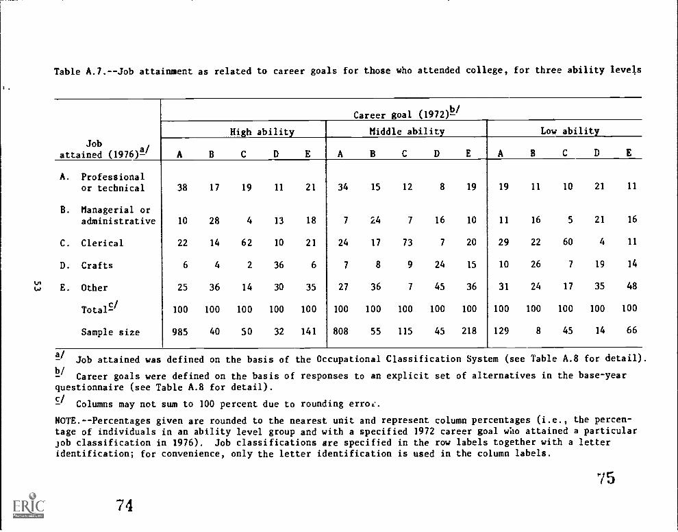
Table A.7.--Job attainment as related to career goals for those who attended college, for three ability levels
Jobattained (1976)x/
Career goal (1972)1
High ability Middle ability Low abilit Y
A B C DE A B C DE A B C D E
A. Professionalor technical 38 17 19 11 21 34 15 12 8 19 19 11 10 21 11
B. Managerial oradministrative 10 28 4 13 18 7 24 7 16 10 11 16 5 21 16
C. Clerical 22 14 62 10 21 24 17 73 7 20 29 22 60 4 11
D. Crafts 6 4 2 36 6 7 8 9 24 15 10 26 7 19 14
t.nw E. Other 25 36 14 30 35 27 36 7 45 36 31 24 17 35 48
Total!/ 100 100 100 100 100 100 100 100 100 100 100 100 100 100 100
Sample size 985 40 50 32 141 808 55 115 45 218 129 8 45 14 66
a/Job attained was defined on the basis of the Occupational Classification System (see Table A.8 for detail).
b/Career goals were defined on the basis of responses to an explicit set of alternatives in the base-year
questionnaire (see Table A.8 for detail)./
Columns may not sum to 100 percent due to rounding error.
NOTE.--Percentages given are rounded to the nearest unit and represent column percentages (i.e., the percen-tage of individuals in an ability level group and with a specified 1972 career goal Wilo attained a particularjob classification in 1976). Job classifications are specified in the row labels together with a letteridentification; for convenience, only the letter identification is used in the column labels.
"/5
74
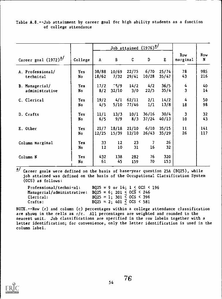
Table A.8.--Job attainment by career goal for high ability students as a functionof college attendance
Career goal (1972)A/
College
Job attained (1976)A/
Rowmarginal
RowNA
A. Professional/ Yes 38/88 10/69 22/75 6/70 25/74 78 985
technical No 18/62 7/32 29/41 10/28 35/47 43 216
B. Managerial/ Yes 17/2 73/9 14/2 4/2 36/5 4 40
administrative No 8/2 32/10 3/0 22/5 35/4 3 14
C. Clerical Yes 19/2 4/1 62/11 2/1 14/2 4 50No 4/5 5/10 77/46 1/1 13/8 18 98
D. Crafts Yes 11/1 13/3 10/1 36/16 30/4 3 32
No 6/5 9/9 8/3 37/24 40/13 10 43
E. Other Yes 21/7 18/18 21/10 6/10 35/15 11 141
No 12/25 15/39 12/10 26/43 35/29 26 117
Column marginal Yes 33 12 23 7 26
No 12 10 31 16 32
Column N Yes 432 138 282 76 320
No 61 45 159 70 153
A/ Career goals were defined on the basis of base-year question 25A (BQ25), whilejob attained was defined on the basis of the Occupational Classification System(OCS) as follows:
Professional / technical: BQ25 = 9 or 14; 1 < OCS < 196Managerial/administrative: BQ25 = 6; 201 < OCS < 246Clerical: BQ25 = 1; 301 < OCS < 396
Crafts: BQ25 = 2; 401 < OCS < 581
NOTE.--Row Cr) and column (c) percentages within a college attendance classificationare shown in the cells as r/c. All percentages are weighted and rounded to thenearest unit. Job classifications are specified in the row labels together with aletter identification; for convenience, only the letter identification is used in thecolumn label.
754
76
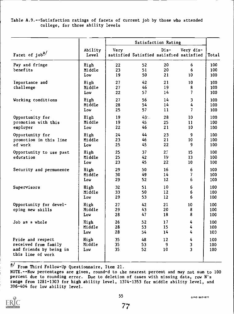
Table A.9.--Satisfaction ratings of facets of current job by those who attendedcollege, for three ability levels
Facet of joba/
Pay and fringebenefits
Importance andchallenge
Working conditions
Opportunity forpromotion with thisemployer
Opportunity forpromotion in this lineof work
Opportunity to use pasteducation
Security and permanence
Supervisors
Opportunity for devel-oping new skills
Job as a whole
Pride and respectreceived from familyaad friends by being inthis line of work
Satisfaction Rating
AbilityLevel
Very Dis- Very dis-satisfied Satisfied satisfied satisfied Total
High 22 52 20 6 100
Middle 23 51 20 6 100
Low 19 50 21 10 100
High 27 42 21 10 100
Middle 27 46 19 8 100
Low 22 57 14 7 100
High 27 56 14 3 100
Middle 28 54 14 4 100
Low 25 57 11 7 100
High 19 43-- 28 10 100
Middle 19 45 25 11 100
Low 22 46 21 10 100
High 24 44 23 9 100
Middle 23 46 21 10 100
Low 25 45 22 9 100
High 25 37 2: 15 100
Middle 25 42 19 13 100
Low 23 45 22 10 100
High 29 50 16 6 100
Middle 30 49 14 7 100
Low 29 52 12 6 100
High 32 51 10 6 100
Middle 33 50 12 6 100
Low 29 53 12 6 100
High 27 42 21 10 100
Middle 29 43 20 8 100
Low 28 47 18 8 100
High 26 52 17 4 100
Middle 28 53 15 4 100
Low 28 54 14 4 100
High 35 48 12 4 100Middle 35 53 9 3 100
Low 35 52 10 3 100
a/From Third Follow-Up Questionnaire, Item 21.
NOTE.--Row percentages are given, round^d to the nearest percent and may not sum to 100percent due to rounding error. Due to deletion of cases with missing data, row N'srange from 1281-1303 for high ability level, 1374-1353 for middle ability level, and396-404 for low ability level.
55
77GPO 87-071
Recommended