1
Do happiness indexes truly reveal happiness?
Measuring happiness using revealed
preferences from migration flows
Helena Marques
Universidad de las Islas Baleares
Spain
Gabriel Pino
Southern Illinois University
USA
J.D. Tena
Universita di Sassari, Italy and
Universidad Carlos III, Spain
2
Abstract
In this paper we attempt to establish a nexus between migration decisions and self-assessed
happiness, where migration is taken as a mechanism for revealing preferences. The happiness
literature has proposed both economic and non-economic determinants of happiness which
are very similar to the factors that may be thought of as determinants of migration: absolute
income, relative income, demographic and social characteristics, social development,
relationship with others and characteristics of the place where we live. To these we add
bilateral gravity variables, migration policies, and two survey-based happiness indexes. First,
these two indexes are negatively correlated to net migration flows. Second, almost all the
other explanatory variables are significant and as such survey-based happiness indexes fail to
account for them. Third, we show how an international happiness ranking changes by taking
into account those omitted factors. Finally, our migration-based ranking shows that, although
many countries “truthfully” reveal happiness levels, in fact 19 countries are net migration
senders even though they are self-proclaimed happy in surveys, whereas 23 countries are net
migration recipients, even though in surveys they are self-proclaimed unhappy. We identify
the sources of this mismatch and suggest where action could be taken to bring people’s self-
assessment of happiness in line with revealed preferences.
Keywords: happiness, subjective wellbeing, revealed preferences, migration, gravity models,
FEVD
JEL codes: F22,D03,C11,C23
3
1. Introduction
There is a general consensus among academics and politicians on the fact that GDP growth
does not fully capture the level of welfare in a country (see Fleurbaey (2009) for a recent
survey). Due to this limitation, worldwide happiness surveys are widely used both in academic
research and in the construction of worldwide happiness indexes (Kahneman and Krueger,
2006; Frey, 2008; Easterlin, 2010; MacKerron, 2012). However, most of these indicators are
based on answers to subjective questionnaires and their results are subject to a number of
caveats. First, happiness indexes can be seen as the outcome results to economic and social
policies, and so there are strong incentives by governments to manipulate them. As Frey
(2011) indicates, “What is important will be manipulated by the government”. Moreover, even
if national indexes of happiness are not manipulated by politicians, they are not fully reliable
as they are based on subjective appreciations by individuals that largely depend on their
cultural values and/or different types of cognitive bias.1
For this reason, a natural answer to this question should be based on the revealed preference
principle. However, although holding a referendum on every aspect that involves happiness
would result in prohibitively high transaction costs, it is still possible to analyze the factors that
influence “foot voting”, the most universal and primitive form of revealing preferences. In this
paper we take people’s actions, namely the decision to migrate to another country, as a
mechanism of preference revelation. Our starting hypothesis is that people will migrate if they
perceive that their level of happiness in the destination country will be higher than in the
origin country. On the aggregate, international migration flows will reveal an international
happiness ranking that will allow us to build a new happiness index based on revealed
preferences rather than on happiness surveys. We find the use of revealed preferences more
1 In many cases the answers to questionnaires are irrational for a number of reasons that even the
respondent is not aware of (see for example Tversky and Kahneman (1974)).
4
objective and therefore more reliable than people’s subjective assessment of their own
happiness.
The happiness literature has proposed both economic and non-economic determinants of
happiness which are very similar to the factors that may be thought of as determinants of
migration. Dolan et al (2008) classify those factors into: absolute income, relative income,
demographic and social characteristics, social development, time use, relationship with others
and characteristics of the place where we live. We take into account variables measuring these
various aspects, plus typical bilateral gravity variables (distance, common border, and common
language) and migration policies. This very large pool of (potentially relevant) variables is
included in a panel regression in addition to two typical happiness indexes originated from
survey data. In this way, we are able to show whether the migration decision is correlated with
this index. At the same time we are able to identify the additional factors that the index fails to
measure and consequently how an international happiness ranking changes by taking into
account those omitted factors.
The remainder of the paper is organized as follows: section 2 provides some background on
happiness indexes as usually taken from survey data and determinants of happiness usually
proposed by the happiness literature; section 3 presents the details on the empirical strategy,
which consists of estimating a gravity model of migration to reveal preferences, using the FEVD
panel estimation methodology of the migration gravity model; section 4 presents and
discusses the panel estimation results; section 5 proposes a happiness index based on
preferences revealed through migration. Finally, section 6 concludes.
5
2. Background on happiness indexes and determinants
The use of happiness indexes built from survey data to measure Subjective Wellbeing (SWB)
goes back to the 1970s (Easterlin, 1994).2 The typical survey question that has been repeated
over and over again is: “Are you happy?” (Easterlin, 2001). The answer to this question is
based on the individual’s own assessment and is therefore highly subjective. It is influenced by
moods, perceptions, and general beliefs, which are not comparable across individuals or
countries, and may even be endogenous to the state of happiness itself. As such the findings of
the behavioral economics research that uses happiness indexes based on data from this typical
survey question may not be the most reliable.
Most authors have been trying to circumvent this difficulty by incorporating in surveys more
sophisticated versions of Easterlin’s question. Roysamb et al. (2002), for example, used the
sum-score of four items: a) ``When you think about your life at present, would you say you are
mostly satisfied with your life, or mostly dissatisfied?''; b) ``Are you usually happy or
dejected?''; c) ``Do you mostly feel strong and fit or tired and worn out?''; d)``Over the last
month, have you suffered from nervousness, felt irritable, anxious, tense, or restless?'. This
formulation is an attempt to separate the cognitive aspect of happiness (general life
satisfaction) from the affective aspect (happy, strong, tired, nervous). In turn, Ferrer-i-
Carbonell (2005) used the question from the German Socio Economic Panel (GSEP): “How
happy are you at present with your life as a whole?”, whilst Mentzakis and Moro (2009) used
the question introduced in the British Household Panel Survey (BHPS): “How dissatisfied or
satisfied are you with your life overall?”. Finally, Pedersen y Schmidt (2011) use a question
2 Strictly, subjective well-being includes happiness (the emotional or affective component) and
satisfaction (the cognitive component). However, most authors, including Easterlin and Frey, use the
terms happiness and subjective well-being interchangeably.
6
regarding self-reported satisfaction with work or main activity taken from the European
Community Household Panel (ECHP).
If we move away from the individual’s subjective assessment of happiness and try to build an
objective measure we are faced with an open debate about the determinants of happiness.
For example, Krueger and Shakade (2008) mention that subjective wellbeing research has been
linked to such heterogeneous issues as studies of the tradeoff between inflation and
unemployment, the effect of cigarette taxes on welfare, German reunification, lottery
winnings, labor turnover, productivity or health. A very complete review of the economic
literature associated to human happiness can be found in Dolan et al. (2008). They sort out a
list of all possible factors affecting wellbeing into seven broad groups: (1) absolute and relative
income; (2) personal characteristics; (3) social development characteristics; (4) how we spend
our time; (5) attitudes and beliefs toward self/others life; (6) relationships; and (7) the wider
economic, social and political environment.
The idea that people with higher absolute income levels would report higher levels of
happiness has not been fully supported by the literature. Easterlin’s Paradox says that,
although this should apparently be so, the fact is that wants and aspirations also increase with
income (Easterlin, 1995). Since individuals report happiness levels relative to their aspirations,
the reported levels of happiness do not seem to increase with absolute income in empirical
studies. When panel data is used, a positive correlation between happiness and absolute
income appears in the between variation (cross-section dimension), but not in the within
variation (time-series dimension). At the macro level, this would mean that countries with
higher average income levels would appear in an international happiness ranking with higher
average happiness levels, but in one single country an increase in average income levels over
time would not increase the average happiness level (see Blanchflower and Oswald (2004) or
Pedersen and Schmidt (2011)).
7
Easterlin (2001) proposed a correction to solve the Paradox: happiness is more dependent on
relative than on absolute income. This happens because each individual compares her own
income to the average income of her reference group, that is, the socio-economic group with a
similar educational and/or professional level within which the individual maintains her social
relationships. Testing this proposal for German data, Ferrer-i-Carbonell (2005) finds that the
income of the reference group is about as important as the own income for individual
happiness. Individuals are happier the larger their income is in comparison to the average
income of their reference group. For British data, Mentzakis and Moro (2009) consider both
absolute and relative income, also finding the latter to be more relevant for happiness. At the
macro level, the concept of relative income is related to the level of income inequality within a
country and can be measured by an inequality measure such as the Gini index.
The second group of determinants of happiness suggested by Dolan et al. (2008) is formed by
personal characteristics such as age, gender, ethnicity, household size, number of kids,
education and marital status. Peiró (2006) finds that age, health and marital status are strongly
associated with happiness and satisfaction. In addition, Roysamb et al. (2002) find that women
are, on average, happier than men. Moreover, happiness tends to follow a U-curve with age,
reaching a minimum around 35-40 years old (see, for example, Blanchflower and Oswald
(2008), Mentzakis and Moro (2009), and Realo and Dobewall (2011)). Further, Pedersen and
Schmidt (2011) find that the level of and change in self-reported health has a strong impact on
satisfaction.
A third group concerns social development characteristics, which include education, health (or
life expectancy), sector of work (agriculture, manufacturing, services), unemployment. Peiró
(2006) finds that unemployment does not appear to be associated with happiness, although it
is clearly associated with satisfaction. This is because income is strongly associated with
satisfaction, but its association with happiness is weaker. These results point to happiness and
8
satisfaction as two distinct spheres of well-being. While the first would be relatively
independent of economic factors, the second would be strongly dependent on them.
Moreover, Pedersen and Schmidt (2011) find a strong negative impact on satisfaction from
being unemployed and a somewhat weaker impact from being inactive, supposedly because
the latter depends more on a deliberate choice by the individual.
Fourth, how we spend our time can be described by variables such as hours worked,
commuting, care for others, community involvement and volunteering, and religion activities.
At the macro level, a great deal of these behaviours is shaped by factors such as the dominant
religion in a country.
Fifth, the characteristics of relationships with others can be described with respect to marriage
and intimate relationships, family and friends. At the macro level, relationship attitudes can be
proxied by the percentage of married and single people in a country, importance given to
family and friends, population density or urban/rural location.
Finally, the wider economic, social and political environment is represented by a variety of
country characteristics such as inflation, welfare system and public insurance, economic
freedom, climate, natural environment, safety, political freedom and nature of policies. Among
these, a factor of concern in many countries is the phenomenon of terrorism, which has been
studied by Abadie (2006) and Abadie and Gardeazabal (2008). At the macro level, Peiró (2006)
examines the relationship between socio-economic conditions and happiness in 15 countries.
Finally, relevant sport events are incorporated to examine their possible impact on Happiness
as some recent literature suggests (see for example Kavetsos and Szymanski, 2010).
The purpose of this paper is to further contribute to the move towards an objective measure
of happiness. This is done using revealed preferences through migration choices and taking
9
into account the determinants of happiness described previously. The detailed explanation of
the empirical strategy followed in this paper is the object of the next section.
3. Empirical strategy
3.1. The revelation of preferences through migration
The aim of this paper is to provide an objective measure of happiness at the country level
using preferences revealed through migration flows. We conjecture that ceteris paribus
countries with higher happiness levels attract more migrants and thus migration flows should
contain information about country-level average happiness. The migration literature at the
country level has traditionally used gravity models to account for the determinants of
migration flows (see, for example, the recent work by Felbermayr and Toubal (2012), or
Hanson and McIntosh (2012)). Gravity models relate bilateral flows of trade, investment, or in
our case, migration, to the size of the partner countries and the inverse of the distance
between them. More generally, the gravity literature includes a number of variables capturing
factors that facilitate or hinder migration. Among them, our focus variables are those
somehow linked to subjective wellbeing and described in section 2.
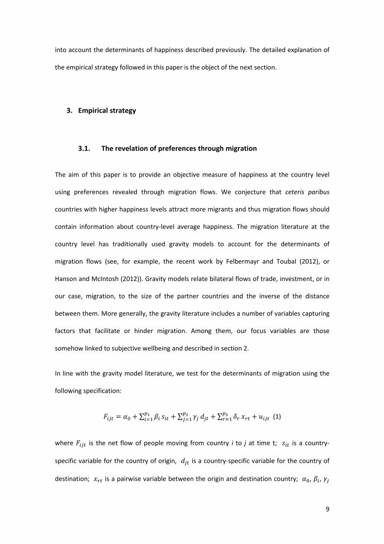
In line with the gravity model literature, we test for the determinants of migration using the
following specification:
���� � �� � ∑ ���� � ��� � ∑ ��
��� � ��� � ∑ ��
��� � ��� � ���� (1)
where ���� is the net flow of people moving from country i to j at time t; ��� is a country-
specific variable for the country of origin, ��� is a country-specific variable for the country of
destination; ��� is a pairwise variable between the origin and destination country; ��, �, ��
10
and �� are parameters of the model; and ���� is an iid error with zero mean and �� variance
for countries i and j at time t.
In particular, the pairwise variables in our model are the distance between each pair of
countries, and two dummy variables that take value 1 when the pair of countries shares a
common language and a common border respectively and zero otherwise.
In the course of data collection we were faced with a large number of missing values for the
explanatory variables and even for the dependent variables, particularly for very small
countries and for pairs of countries between which there are no migration flows. The problem
of missing data brings up the need to distinguish between a missing value and a zero flow,
which might introduce selection effects and force the use of a Tobit.3 Instead we decided in
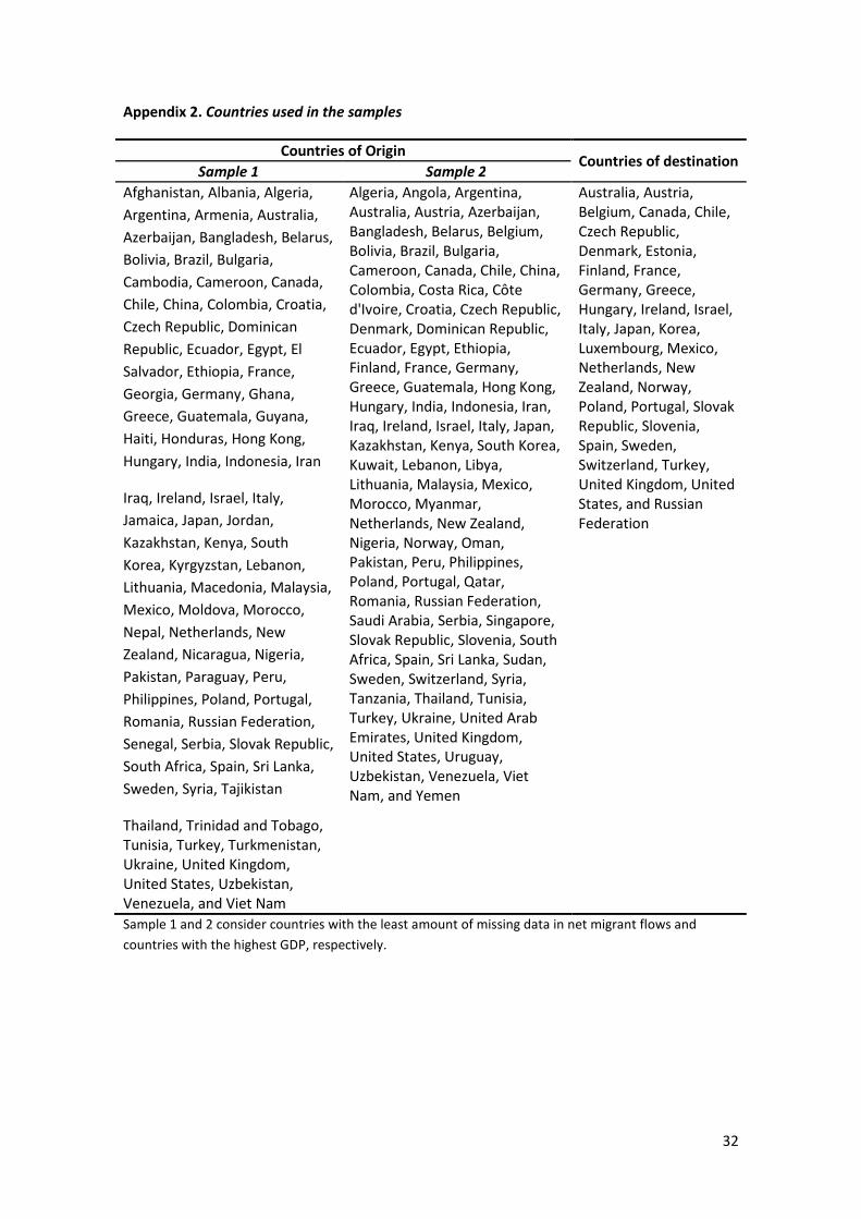
favour of considering two different samples: (i) Sample 1 includes countries with the least
number of missing values in the dependent variable (net migration flows); (ii) Sample 2
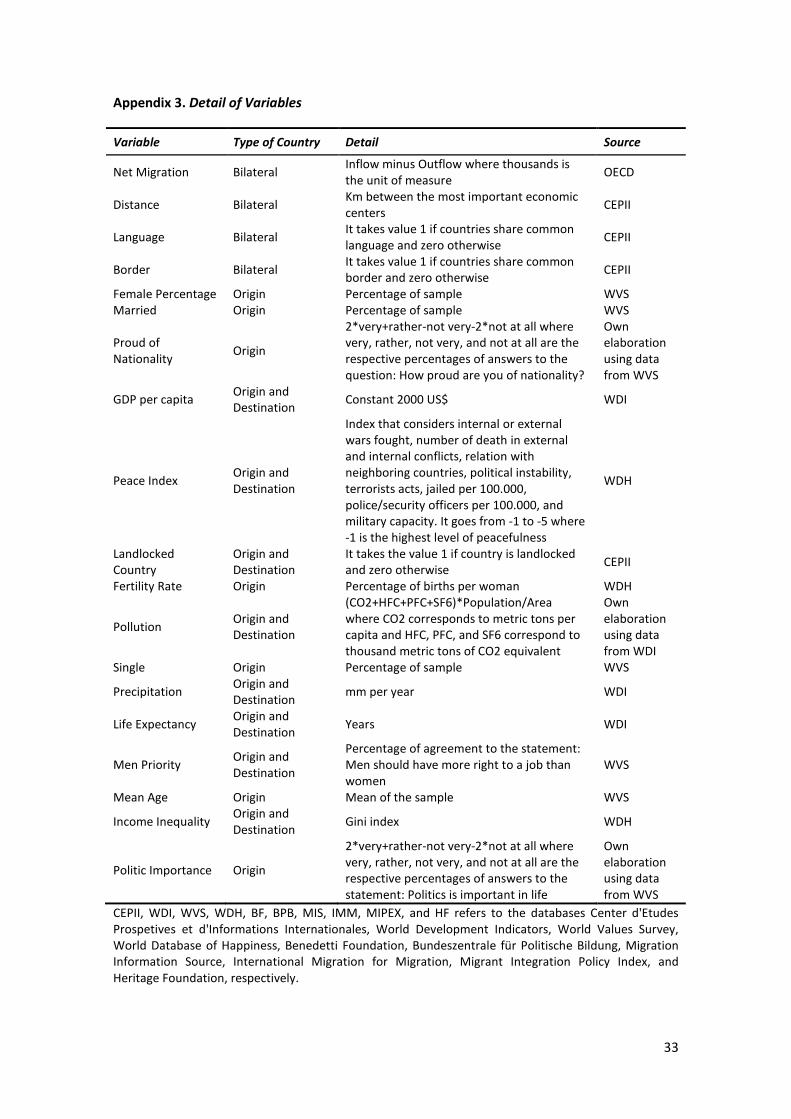
includes the larger countries as measured by GDP. The Appendixes explain in detail the
construction of the samples (Appendix 1), the countries included (Appendix 2) and the final
variables selected (Appendix 3), including the data sources.
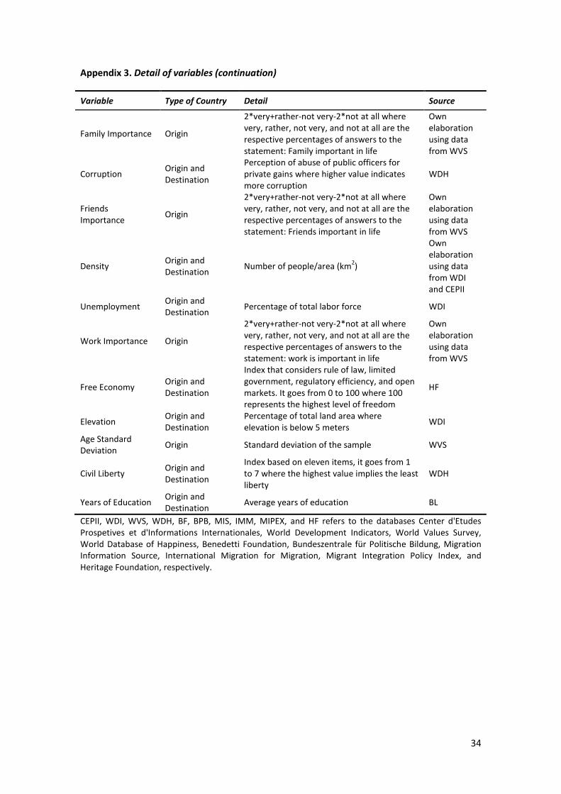
The country-specific variables for the countries of origin and destination have already been
described in section 2 and refer to a wide range of variables that can be thought to be
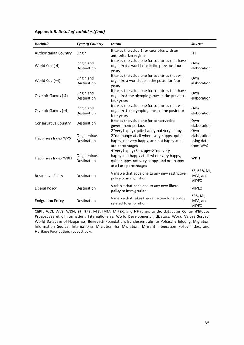
potential determinants of happiness, plus migration policies.4
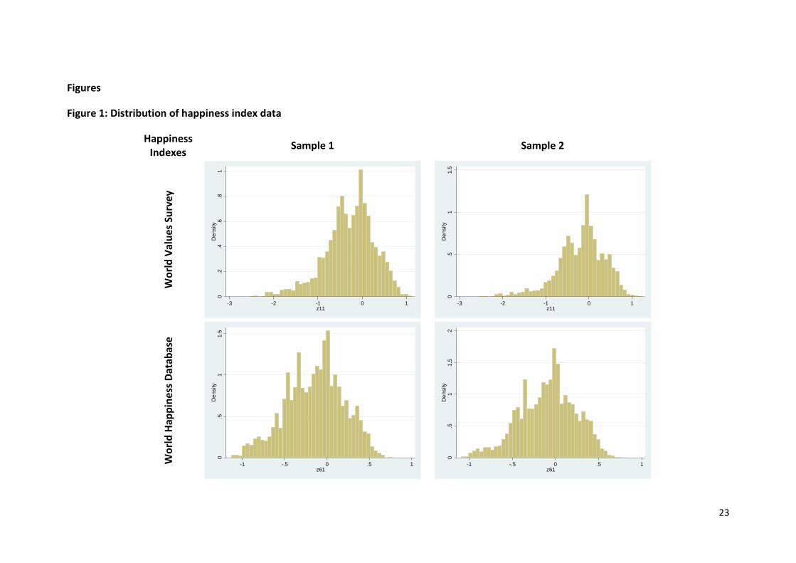
We also explicitly use as explanatory variables two traditional happiness indicators taken from
survey data. We selected two of the most widely cited: (i) Happiness Index 1 from the World
Values Survey (http://www.worldvaluessurvey.org/) carried out by the World Values Survey
3 The investigation of selection effects is still work in progress.
4 Migration policies have been widely used as explanatory variables of the migration decision (see,
among others, Marques (2010) and Egger and Nelson (2012)).
11
Association, a non-profit association based in Stockholm, Sweden; (ii) Happiness Index 2 from
the World Happiness Database (http://www1.eur.nl/fsw/happiness/) built by the Erasmus
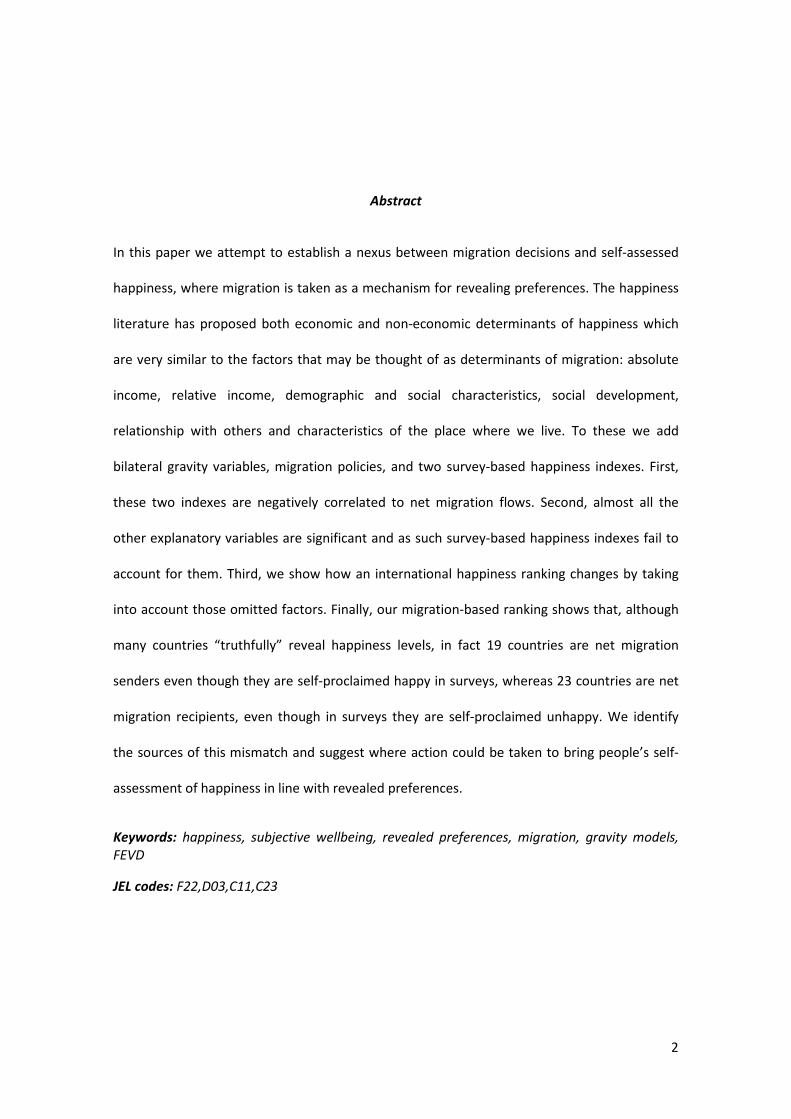
University Rotterdam. Their distribution reveals that most answers cluster around zero with a
tendency towards a slightly negative assessment of happiness: “not very happy” is the answer
chosen by many respondents (see Figure 1 for the histograms of these indexes).5 The
distribution of the two indexes is remarkably similar in both samples, with correlation
coefficients of 0.894 in Sample 1 and 0.888 in Sample 2. The inclusion of these two widely used
indexes in our regressions makes it possible to identify the relationship between the
traditional survey variables and our revealed preference measure (migration) and show the
impact of the additional explanatory variables. The significance of this impact demonstrates
the incompleteness of the traditional happiness indicator.
FIGURE 1 HERE
3.2. FEVD panel estimation
Since both data samples constitute a panel, we are able to exploit panel data features instead
of following the cross-section structure typical of the research that uses happiness indicators
from survey data. For example, the use of panel data allows us to exploit the time-series
dimension and make use of lagged variables to account for endogeneity, similarly to what
Mentzakis and Moro (2009) had done for self-assessed health and unemployment, although
these authors had used an ordinal SWB index. Indeed, whereas happiness indicators from
surveys are ordinal, our dependent variable is quantitative (cardinal) and, more importantly, it
5 The index provided by the World Values Survey is given by a weighted average of the percentage of
each answer calculated as 2*very happy + quite happy-not very happy-2*not at all happy. The index
provided by the World Happiness Database considers different answer possibilities to the question
“How happy would you say you are these days?”. The weighted average of the percentage of each
answer is calculated as very happy*4+happy*3+not very happy*2+not at all happy*1.
12
is objective instead of resulting from a subjective self-assessment. Thus we are able to create a
meaningful country ranking. Moreover, by using a panel structure we are able to account for
Easterlin’s Paradox, according to which cross-sectional variations in happiness may not be
matched by time-series variations due to the adjustment of expectations over time (Ferrer-i-
Carbonell and Frijters (2004)).
We start by taking into account the potential correlation between ����, the error component in
equation (1), and the different covariates in the model, by running the standard Hausman
(1978) test based on the difference between the random and fixed effect estimators. The null
hypothesis can be rejected at all the conventional levels for the two samples, which suggests
the convenience of considering a fixed effect model that provides unbiased estimation in this
case. Moreover, by using fixed effects we are able to account for all unobservable factors that
the traditional survey-based cross-section analysis is not able to account for.
However, a traditional fixed effect model eliminates time invariant variables such as distance,
common border and common language, whilst the estimation of the impact of these
covariates on migration is an important part of this analysis. This problem is circumvented by
using the fixed-effects vector decomposition (FEVD henceforth) proposed by Plümper and
Troeger (2007). Breusch et al. (2011) show that this model is just an IV estimator with a
particular set of instruments: the time-invariant variables and the time-variant variables
expressed in deviations with respect to its mean. This estimator is an alternative to the
Hausman and Taylor (1978) model (HT henceforth). The former can be also expressed as an IV
estimator that partitions both time-variant and time-invariant variables into exogenous and
endogenous variables. As explained by Breusch et al. (2011), a consistent estimator such as HT
will be preferable to the FEVD for sufficiently large sample size. However, for small sample size
with a small endogeneity problem, it might be preferable to include time-invariant
13
endogenous variables as instruments as FEVD does.6 Given that none of these procedures
dominate each other we considered both in our analysis for completeness. 7
4. Estimation results
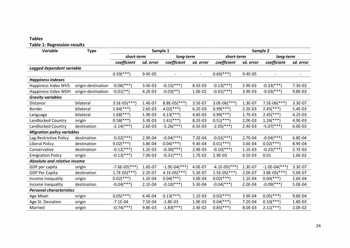
Since the Hausman test confirmed that FEVD should be preferred over HT, the estimation
results for FEVD regressions are presented in Table 1. The signs of the coefficients are robust
across the two samples for the majority of variables. The inclusion of the lagged dependent
variable reveals the significant persistence of the geography of migration flows over time,
which is a common result in the migration literature. Moreover, having a coefficient close to
0.5, suggests that there is no need to incorporate any correction for non-stationarity. Using the
coefficient of the lagged dependent variable, it is possible to obtain long-run coefficients and
their long-run significance for the remaining explanatory variables. The long-run results do not
differ qualitatively from those of the short-run, although the long-run impact amplifies that of
the short-run due to the positive sign of the lagged dependent variable coefficient. The
cumulative nature of this result confirms the high persistence and increasing impact of
migration determinants over time.
TABLE 1 HERE
The two survey-based happiness indexes mentioned in section 3 are negatively correlated to
migration flows. Simple correlation coefficients vary between -0.078 (Sample 2) and -0.043
(Sample 1) for the World Values Survey index and -0.057 (Sample 2) and -0.028 (Sample 1) for
6 The issue of endogeneity is further handled by introducing lagged values for some variables.
7 The HT results are available from the authors upon request. In any case, the signs of the HT coefficients
are the same as for FEVD, although their significance levels are consistently higher using FEVD, which is
also supported by the Hausman test.

14
the World Happiness Database index. These values do not change much after accounting for all
the other factors that impact on migration in Table 1 regressions. This result reveals that
subjective assessments of one’s own happiness are biased and clearly at odds with observed
actions in terms of country preferences revealed through migration. If this was not the case,
countries with a positive self-assessed happiness differential should be net recipients of
migrants. We obtain exactly the opposite result. Further to their biasedness, the main test of
the incompleteness of these happiness indexes is the significance of almost all additional
explanatory variables we consider: traditional gravity variables, migration policy variables, and
various other variables that influence happiness grouped around the broad groups described
in section 2.
In particular, all the traditional gravity model variables are significant at 1%. Migration depends
positively on distance as well as on common border and language. The positive impact of
distance on migration here simply translates the fact that the dependent variables are
migration flows from all corners of the world into OECD countries and more distant countries
supply more migrants. It is however a very small coefficient. Moreover, being a landlocked
country increases migration at origin and decreases it at destination. These are country-level
factors that are not considered in the two survey-based happiness indexes.
When the dependent variable is migration flows it is very important to control for migration
policies. In the destination countries, liberal policies are expected to facilitate and therefore
increase migration flows, whereas restrictive policies should have the opposite effect. Out of
the four variables that measure policies towards migration in the destination countries, three
15
have the expected sign in both samples.8 The emigration policy dummy only applies to Mexico
and Russia and for this reason the sign of its coefficient changes with the sample.9
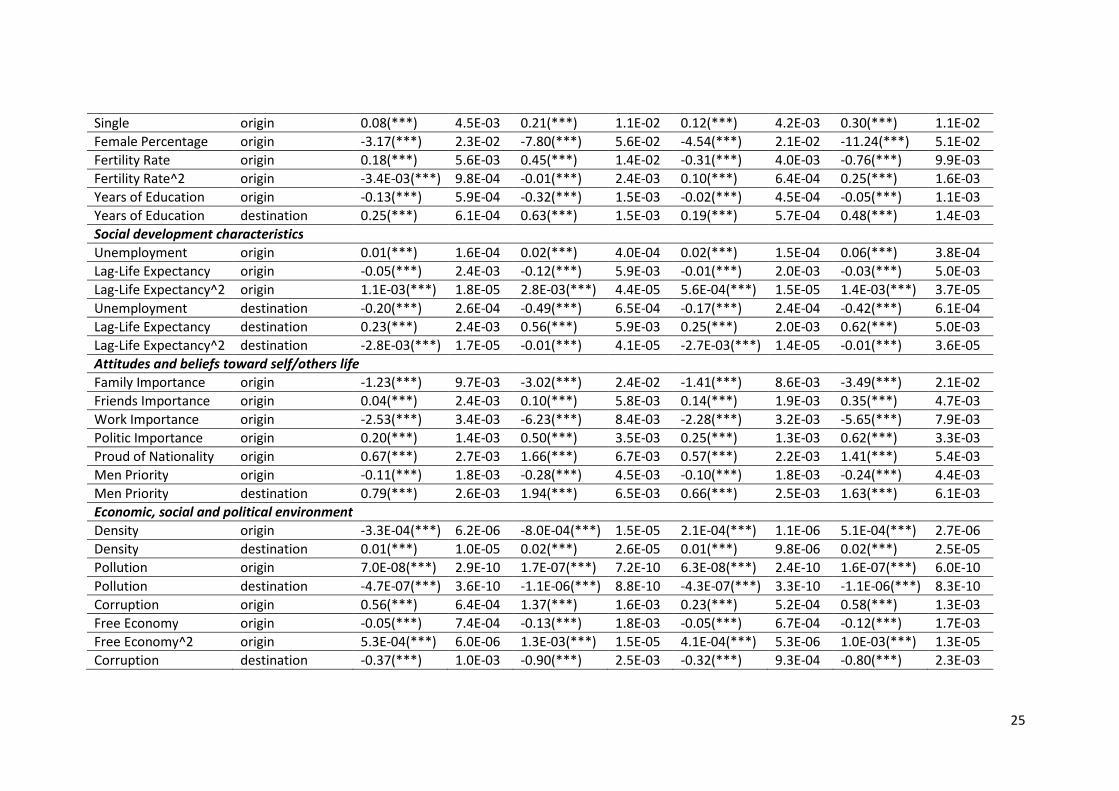
Also significant is a large number of individual and country characteristics which are not taken
into account either by the survey-based happiness indexes or by the traditional gravity
variables. The happiness literature has highlighted the importance of absolute and relative
income and so has the migration literature. Indeed we find that migrants flow from poorer to
richer countries and from more unequal to less unequal countries. Presumably, this is because
both absolute and relative income influence preferences as has been reported by the
happiness literature.
We also control for a number of personal characteristics which are aggregated at the country
level either by taking means or by calculating the percentage of population that bears such
characteristic in the country. The results that are robust across samples show that there is
more emigration from origin countries with higher mean age, higher percentage of single
people, and higher percentage of men in the population. The effect of education at the
destination country is clearly positive. Generally, countries with higher educational levels may
offer broader employment opportunities. Similarly, having higher educational levels decreases
emigration as educated people are more sought after even in their home country. This result
underscores the importance of years of education in the domestic and foreign labour markets.
Next we take into account social development characteristics such as unemployment and life
expectancy. It would be expected that migration would increase (decrease) with
unemployment at the origin (destination). In general, these expectations are confirmed by the
8 Note however that restrictive policy only produces an effect after one period lag. It is likely that
endogeneity is an issue for this variable. Marques (2010) lagged migration policy variables up to two
periods. A similar strategy was used here.
9 Mexico imposed a restrictive emigration policy by applying higher border controls to illegal emigration.
On the contrary, Russia allows the stay of Russian nationals in Lithuania for up to 30 days without visa.
16
results. Life expectancy is a more complex variable because countries where people live longer
supply more migrants over time but on the other hand provide less labour market vacancies.
To account for endogeneity and non-linearity, this variable was lagged one period and its
square was included as an additional explanatory variable. After carrying out these
modifications, life expectancy is found to decrease (increase) migration at the origin
(destination) but at a decreasing rate in both cases. These results are consistent with the
hypothesis that life expectancy proxies for general well-being in a country rather than
representing labour market considerations.
Another group of factors influencing country preferences would be the migrant’s attitudes and
beliefs. For example, there is more emigration out of countries where more people attribute
more importance to friends and politics, as well as being proud of their nationality. Perhaps
this result is due to the migrants having friends abroad or going abroad too, and also to
migration being more likely the more the migrants are attuned to politics or nationality. On the
contrary, there is less emigration out of countries where higher average importance is given to
family and work. The result that migration diminishes (increases) with the level of priority
given to men in the origin (destination) country seems to imply that the majority of migrants
are men, which seems plausible at the world level.
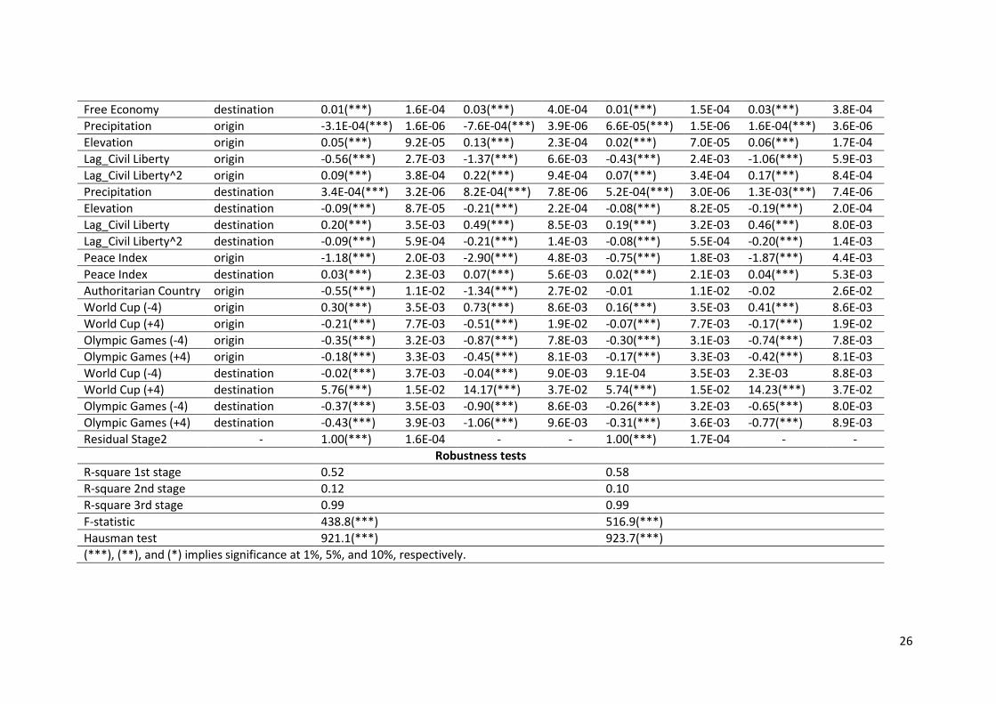
The final group of variables concerns several general country characteristics that make them
more or less attractive. The results indicate that there is more emigration out of countries with
more pollution, higher altitude, more corruption, less peaceful, less civil liberties,10 and more
authoritarian regimes. These are all undesirable characteristics for most people. On the
contrary, emigration is lower out of countries with a freer economy, although this effect
stabilizes with the degree of freeness. On the other hand, immigration is higher into countries
10
This variable also presents endogeneity and non-linearities. Both at origin and at destination its effect
operates at a decreasing rate.
17
with higher population density, lower pollution, higher rainfall, lower altitude, lower
corruption levels, and a freer economy. Indeed, many of these variables are simply proxies for
a high level of economic activity and social interaction, therefore better employment
opportunities.
The final set of variables relates to the organization of World Cups or Olympic Games in the
previous four years and its taking place within four future years. Generally, hosting the World
Cup or the Olympics reduces emigration out of a country. It also increases immigration into the
organizing country in the case of a forthcoming World Cup, but paradoxically it is a negative
incentive to immigration in the case of the Olympics. There is in any case a lack of consensus
regarding the role of these variables in the happiness literature (see the discussion in Kavetsos
and Szymanski, 2010).
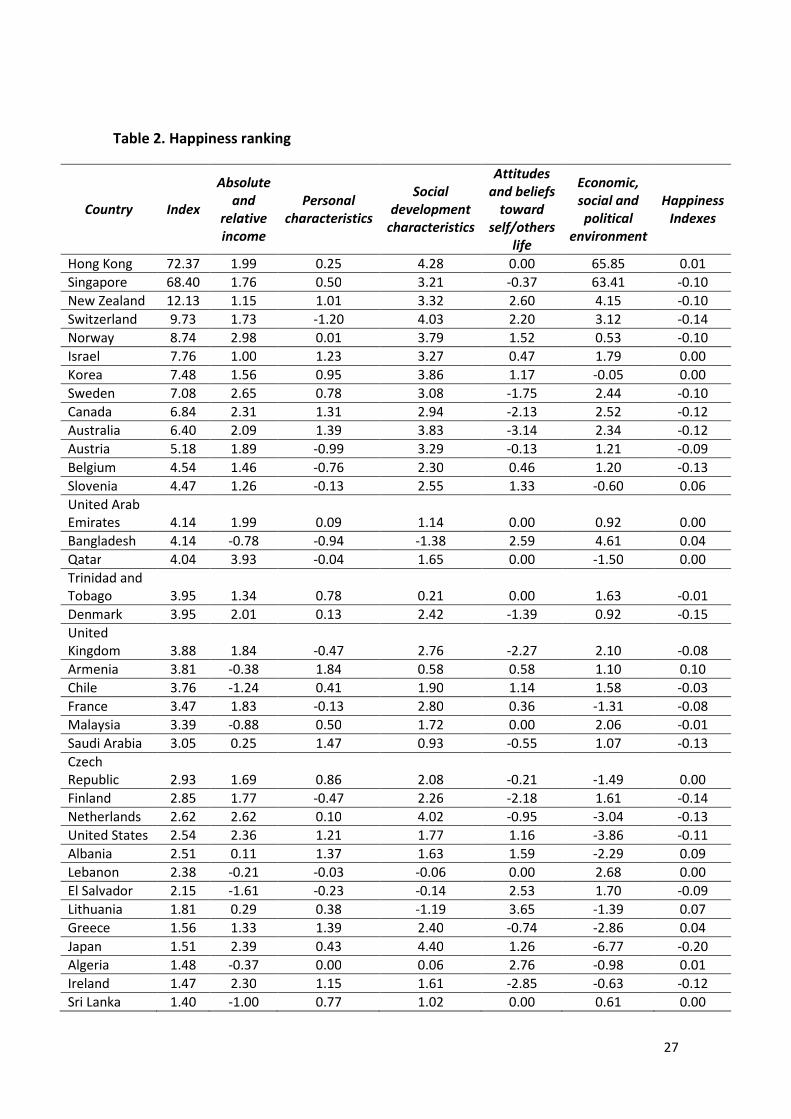
5. A proposal for a happiness index based on revealed preferences
The previous results have shown that happiness indexes based on surveys are insufficient to
explain why people prefer some countries over others. Moreover, individuals’ own assessment
of their happiness is at odds with their actions, that is, their cross-country flows. Since we are
taking migration flows as a mechanism of preference revelation, it is natural to see countries
that are net recipients of migrants as happier countries. In this sense, we take the estimation
results from the previous section and use them to build a happiness index based on revealed
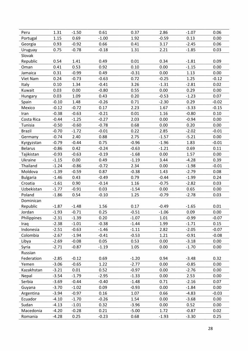
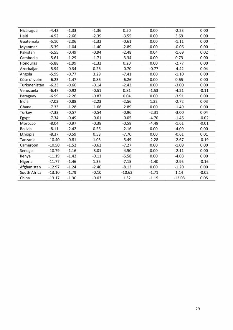
preferences through migration. The index is presented in Table 2 for the full predicted
migration flows and for the five variable groups that influence happiness and discussed in the
previous section. The final column of Table 2 provides the average value of the two survey-
based happiness indexes.
TABLE 2 HERE
18
The values presented in Table 2 result from an averaging of coefficients and values taken by
explanatory variables across the two samples. The coefficients themselves are the mean point
of a confidence interval and themselves represent a mean behavior. Therefore, in interpreting
the index values for each country, an ordinal rather than a cardinal perspective should be
employed. For many countries, a positive value of the survey-based indexes (average positive
self-assessed happiness in the country) is matched by positive net migration flows (average net
desirability of the country).
The most interesting cases are those for which average self-assessed happiness and average
observed net desirability are clearly at odds. Here we distinguish two main types of countries:
those self-proclaimed happy but regarded as undesirable (19 mostly middle-income and
emerging economies), and those self-proclaimed unhappy but regarded as desirable (23
mostly high-income countries). The study of the five groups of determinants of happiness
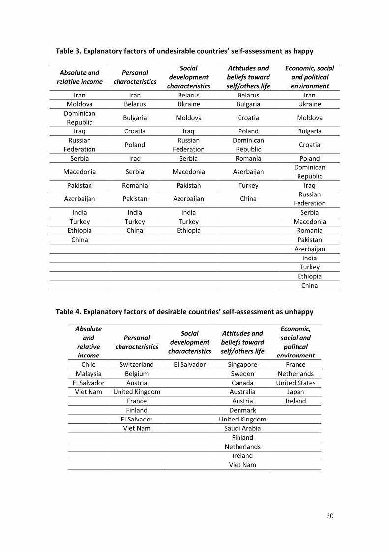
reveals why this mismatch occurs (see Tables 3 and 4).
TABLE 3 HERE
TABLE 4 HERE
Table 3 countries fare poorly on issues of economic, social and political environment, as well as
on absolute and relative income in most cases, but some of them achieve a positive score on
attitudes and beliefs. These are countries with a difficult recent history, not typically sought
after as a place of residence by foreign nationals, but where their own nationals’ attitudes and
beliefs may lead them to regard themselves as happy.
Table 4 countries seem to group into two different cases. On the one hand, there are middle-
income countries whose economy is emerging fast, but which fare poorly in terms of average
absolute income and income inequality. These countries are sought after from outside, but
their nationals are still negatively affected by income issues. As growth continues and income
19
inequality is dealt with, these countries may in the future join those that are both sought after
and self-declared happy. On the other hand, there is a group of high-income countries where
attitudes and beliefs make their nationals self-assess as unhappy, even though these countries
are sought after from abroad. Within these, five countries (France, Netherlands, United States,
Japan and Ireland) also fare poorly in terms of economic, social and political environment. If
these aspects were improved, these countries’ citizens’ self-assessment of happiness might in
the future be brought in line with their countries’ international popularity.
6. Conclusions
In this paper we attempt to establish a nexus between migration decisions and self-assessed
happiness, where migration is taken as a mechanism for revealing preferences. We estimate
the impact of a large and diverse number of variables on migration flows, in addition to two
survey-based indexes widely used to rank country happiness. Applying a FEVD estimation
methodology to a gravity model specification for a large panel dataset, we are able to estimate
both short and long-run coefficients for the explanatory variables. Using these estimated
coefficients, we build an alternative ranking based on revealed preferences.
The estimation results reveal that the two survey-based indexes provide biased and
incomplete results. Moreover, the migration-based ranking shows that, although many
countries “truthfully” reveal happiness levels, in fact 19 countries are net migration senders
even though they are self-proclaimed happy in surveys, whereas 23 countries are net
migration recipients, even though in surveys they are self-proclaimed unhappy. Inspection of
the role played by the five groups of determinants of happiness included in the regressions
reveals that the former group has a poor economic, social and political environment, as well as
absolute and relative income issues. Their high score on attitudes and beliefs may lead them to
20
regard themselves as happy, but to be able to join those that are both sought after and self-
declared happy they need to improve on their lagging issues. The latter group contains both
emerging economies that need to improve their average income level and decrease income
inequality, and high-income countries where attitudes and beliefs make their nationals self-
assess as unhappy. In some cases the reasons for this low self-assessment are linked to the
economic, social and political environment.
There is still room for improvement in our analysis and a more detailed investigation of the
robustness of our ranking is required. Nevertheless, any ranking of this type should be looked
at under an ordinal rather than a cardinal perspective. Our ranking has the additional
advantage of being based on an objective variable that is not subject to personal evaluation.
An additional contribution lies in identifying where action could be taken to bring people’s self-
assessment of happiness in line with revealed preferences. In any case, it is clear that a
mismatch exists and that survey-based happiness indexes are both biased and incomplete.
References
Abadie, A. (2006), “Poverty, political freedom, and the roots of terrorism”, American
Economic Review, Papers and Proceedings, 96 (2), 50–56.
Abadie, A. and Gardeazabal, J. (2008), “Terrorism and the world economy”, European
Economic Review, 52, 1–27.
Blanchflower, D. and Oswald, A. (2004), “Well-being over time in Britain and the USA”,
Journal of Public Economics, 88, 1359–1386.
Blanchflower, D. and Oswald, A. (2008), “Is well-being U-shaped over the life cycle?”,
Social Science & Medicine, 66, 1733-1749.
Breusch, T., Ward, M.B., Nguyen, H.T.M. and Kompas, T. (2011). “On the fixed-effect
vector decomposition”, Political Analysis, 19, 123-134.
Dolan, P., Peasgood, T., and White,M. (2008). “Do we really know what makes us
happy? A review of the economic literature on the factors associated with subjective well-
being”, Journal of Economic Psychology, 29, 94-122.
21
Easterlin, R.A. (1974), “Does economic growth improve the human lot? Some empirical
evidence”, In: David, P.A., Reder, M.W. (Eds.), Nations and Households in Economic Growth:
Essays in Honour of Moses Abramowitz, Academic Press, New York.
Easterlin, R.A. (1995), “Will raising the incomes of all increase the happiness of all?”,
Journal of Economic Behavior and Organization, 27, 35–47.
Easterlin, R. A. (2001), “Income and Happiness: Towards a Unified Theory”, Economic
Journal, 111, 465-484.
Easterlin, R. A. (2010), Happiness, Growth, and the Life Cycle, New York: Oxford
University Press, 2010.
Egger, P.H. and Nelson, D.R. (2012). "Introduction to Immigration Special Issue of The
World Economy," The World Economy, 35, 107-110.
Felbermayr, G. and Toubal, F. (2012), “Revisiting the Trade-Migration Nexus: Evidence
from New OECD Data”, World Development, 40(5), 928–937.
Fernández, C., Ley, E. and Steel, M. (2001). “Model uncertainty in cross-country growth
regressions”, Journal of Applied Econometrics, 16, 563-576.
Ferrer-i-Carbonell, A. (2005), “Income and well-being: an empirical analysis of the
comparison income effect”, Journal of Public Economics, 89, 997– 1019.
Ferrer-i-Carbonell, A. and Frijters, P. (2004), “The effect of methodology on the
determinants of happiness”, Economic Journal, 114, 641– 659.
Fleurbaey, M. (2009), “Beyond GDP: the quest for a measure of social welfare”,
Journal of Economic Literature, 47, 1029-1075.
Frey, B. (2008), Happiness: a revolution in economics, The MIT Press, Cambridge, MA.
Frey, B. (2011), “Tullock challenges: happiness, revolutions and democracy”, Public
Choice, 148, 269-281.
Hanson, G. and McIntosh, C. (2012), “Birth rates and border crossings: latin-american
migration to the US, Canada, Spain and the UK”, Economic Journal, 122 ( June), 707–726.
Hausman, J.A. (1978). “Specification Tests in Econometrics,” Econometrica, 46, 1251-
1271.
Hausman, J.A. and Taylor, W.E. (1981). “Panel data and unobservable individual
effects”, Econometrica, 49, 1377-1398.
Hoeting, J.A., Madigan, D., Raftery, A.E., and Volinsky, C.T. (1999). “Bayesian Model
Averaging: A Tutorial”, Statistical Science, 14, 382-417.
Kahneman, D. and Krueger, A. (2006), “Developments in the measurement of
subjective wellbeing”, Journal of Economic Perspectives, 20(1), 3–24.
22
Kavetsos, G. and Szymanski, S. (2010). “National well-being and international sports
events”, Journal of Economic Psycology, 31, 158-171.
Krueger, A.B. and Schakade, D.A. (2008). “The reliability of subjective well-being
measures”, Journal of Public Economics, 92, 1833-1845.
MacKerron, G. (2012), “Happiness Economics from 35000 Feet”, Journal of Economic
Surveys, 26(4), 705–735.
Marques, H., (2010). “Migration Creation and Diversion in the EU: any crowding-out
effects from the CEECs?”, Journal of Common Market Studies, 48, 265-90.
Mentzakis, E. and Moro, M. (2009), “The poor, the rich and the happy: Exploring the
link between income and subjective wellbeing”, Journal of Socio-Economics, 38, 147–158.
Pedersen, P. and Schmidt, T. (2011), “Happiness in Europe: Crosscountry differences in
the determinants of satisfaction with main activity”, Journal of SocioEconomics, 40, 480–489.
Peiró, A. (2006), “Happiness, satisfaction and socio-economic conditions: Some
international evidence”, Journal of Socio-Economics, 35, 348–365.
Plümber, T. and Troeger, V. (2007). “Efficient estimation of the time-invariant and
rarely changing variables panel analysis with unit fixed effects”, Political Analysis, 15, 124-139.
Realo, A. and Dobewall, H. (2011), “Does life satisfaction change with age? A
comparison of Estonia, Finland, Latvia, and Sweden”, Journal of Research in Personality, 45,
297–308.
Roysamb, E., Harris, J. and Magnus, P. (2002), “Subjective well-being. Sex-specific
effects of genetic and environmental factors”, Personality and Individual Differences, 32, 211-
223.
Stock, J., and Watson, M. (2002). “Macroeconomic forecasting using diffusion
indexes”, Journal of Business & Economic Statistics, 20, 147−162.
Tversky, A. and Kahneman, D. (1974). “Judgement under uncertainty: Heuristics and
biases”, Science, 185, 1128-1130.
23
Figures
Figure 1: Distribution of happiness index data
Happiness
Indexes Sample 1 Sample 2
Wo
rld
Va
lue
s S
urv
ey
Wo
rld
Ha
pp
ine
ss D
ata
ba
se
0.2
.4.6
.81
De
nsity
-3 -2 -1 0 1z11
0.5
11.
5D
ens
ity
-3 -2 -1 0 1z11
0.5
11.
5D
ens
ity
-1 -.5 0 .5 1z61
0.5
11.
52
De
nsity
-1 -.5 0 .5 1z61
24
Tables
Table 1: Regression results
Variable Type Sample 1 Sample 2
short-term long-term short-term long-term
coefficient sd. error coefficient sd. error coefficient sd. error coefficient sd. error
Lagged dependent variable
0.59(***) 9.4E-05 - - 0.60(***) 9.4E-05 - -
Happiness Indexes
Happiness Index WVS origin-destination -0.06(***) 3.4E-03 -0.15(***) 8.5E-03 -0.13(***) 2.9E-03 -0.33(***) 7.3E-03
Happiness Index WDH origin-destination -0.01(**) 4.2E-03 -0.03(**) 1.0E-02 -0.01(***) 3.9E-03 -0.03(***) 9.8E-03
Gravity variables
Distance bilateral 3.5E-05(***) 1.4E-07 8.8E-05(***) 3.5E-07 3.0E-06(***) 1.3E-07 7.5E-06(***) 3.3E-07
Border bilateral 1.64(***) 2.6E-03 4.02(***) 6.2E-03 0.99(***) 2.2E-03 2.45(***) 5.4E-03
Language bilateral 1.68(***) 1.9E-03 4.13(***) 4.6E-03 0.99(***) 1.7E-03 2.45(***) 4.2E-03
Landlocked Country origin 0.58(***) 3.3E-03 1.41(***) 8.2E-03 0.51(***) 2.0E-03 1.26(***) 4.9E-03
Landlocked Country destination -2.14(***) 2.6E-03 -5.26(***) 6.5E-03 -2.05(***) 2.4E-03 -5.07(***) 6.0E-03
Migration policy variables
Lag-Restrictive Policy destination -0.02(***) 2.9E-04 -0.04(***) 7.2E-04 -0.02(***) 2.7E-04 -0.04(***) 6.8E-04
Liberal Policy destination 0.02(***) 3.8E-04 0.04(***) 9.4E-04 0.01(***) 3.6E-04 0.02(***) 8.9E-04
Conservative destination -0.12(***) 1.2E-03 -0.30(***) 2.9E-03 -0.10(***) 1.1E-03 -0.25(***) 2.7E-03
Emigration Policy origin -0.13(***) 7.0E-03 -0.31(***) 1.7E-02 2.9E-03 6.5E-03 0.01 1.6E-02
Absolute and relative income
GDP per capita origin -7.6E-05(***) 1.6E-07 -1.9E-04(***) 4.0E-07 -4.1E-05(***) 1.3E-07 -1.0E-04(***) 3.3E-07
GDP Per Capita destination 1.7E-05(***) 2.2E-07 4.1E-05(***) 5.3E-07 1.5E-05(***) 2.0E-07 3.8E-05(***) 5.0E-07
Income Inequality origin 0.02(***) 1.2E-04 0.04(***) 3.0E-04 0.02(***) 1.1E-04 0.04(***) 2.6E-04
Income Inequality destination -0.04(***) 2.1E-04 -0.10(***) 5.3E-04 -0.04(***) 2.0E-04 -0.09(***) 5.0E-04
Personal characteristics
Age Mean origin 0.05(***) 4.4E-04 0.13(***) 1.1E-03 0.02(***) 3.9E-04 0.05(***) 9.8E-04
Age St. Deviation origin -7.1E-04 7.5E-04 -1.8E-03 1.9E-03 0.04(***) 7.2E-04 0.10(***) 1.8E-03
Married origin -0.74(***) 9.8E-03 -1.83(***) 2.4E-02 0.85(***) 8.0E-03 2.11(***) 2.0E-02
25
Single origin 0.08(***) 4.5E-03 0.21(***) 1.1E-02 0.12(***) 4.2E-03 0.30(***) 1.1E-02
Female Percentage origin -3.17(***) 2.3E-02 -7.80(***) 5.6E-02 -4.54(***) 2.1E-02 -11.24(***) 5.1E-02
Fertility Rate origin 0.18(***) 5.6E-03 0.45(***) 1.4E-02 -0.31(***) 4.0E-03 -0.76(***) 9.9E-03
Fertility Rate^2 origin -3.4E-03(***) 9.8E-04 -0.01(***) 2.4E-03 0.10(***) 6.4E-04 0.25(***) 1.6E-03
Years of Education origin -0.13(***) 5.9E-04 -0.32(***) 1.5E-03 -0.02(***) 4.5E-04 -0.05(***) 1.1E-03
Years of Education destination 0.25(***) 6.1E-04 0.63(***) 1.5E-03 0.19(***) 5.7E-04 0.48(***) 1.4E-03
Social development characteristics
Unemployment origin 0.01(***) 1.6E-04 0.02(***) 4.0E-04 0.02(***) 1.5E-04 0.06(***) 3.8E-04
Lag-Life Expectancy origin -0.05(***) 2.4E-03 -0.12(***) 5.9E-03 -0.01(***) 2.0E-03 -0.03(***) 5.0E-03
Lag-Life Expectancy^2 origin 1.1E-03(***) 1.8E-05 2.8E-03(***) 4.4E-05 5.6E-04(***) 1.5E-05 1.4E-03(***) 3.7E-05
Unemployment destination -0.20(***) 2.6E-04 -0.49(***) 6.5E-04 -0.17(***) 2.4E-04 -0.42(***) 6.1E-04
Lag-Life Expectancy destination 0.23(***) 2.4E-03 0.56(***) 5.9E-03 0.25(***) 2.0E-03 0.62(***) 5.0E-03
Lag-Life Expectancy^2 destination -2.8E-03(***) 1.7E-05 -0.01(***) 4.1E-05 -2.7E-03(***) 1.4E-05 -0.01(***) 3.6E-05
Attitudes and beliefs toward self/others life
Family Importance origin -1.23(***) 9.7E-03 -3.02(***) 2.4E-02 -1.41(***) 8.6E-03 -3.49(***) 2.1E-02
Friends Importance origin 0.04(***) 2.4E-03 0.10(***) 5.8E-03 0.14(***) 1.9E-03 0.35(***) 4.7E-03
Work Importance origin -2.53(***) 3.4E-03 -6.23(***) 8.4E-03 -2.28(***) 3.2E-03 -5.65(***) 7.9E-03
Politic Importance origin 0.20(***) 1.4E-03 0.50(***) 3.5E-03 0.25(***) 1.3E-03 0.62(***) 3.3E-03
Proud of Nationality origin 0.67(***) 2.7E-03 1.66(***) 6.7E-03 0.57(***) 2.2E-03 1.41(***) 5.4E-03
Men Priority origin -0.11(***) 1.8E-03 -0.28(***) 4.5E-03 -0.10(***) 1.8E-03 -0.24(***) 4.4E-03
Men Priority destination 0.79(***) 2.6E-03 1.94(***) 6.5E-03 0.66(***) 2.5E-03 1.63(***) 6.1E-03
Economic, social and political environment
Density origin -3.3E-04(***) 6.2E-06 -8.0E-04(***) 1.5E-05 2.1E-04(***) 1.1E-06 5.1E-04(***) 2.7E-06
Density destination 0.01(***) 1.0E-05 0.02(***) 2.6E-05 0.01(***) 9.8E-06 0.02(***) 2.5E-05
Pollution origin 7.0E-08(***) 2.9E-10 1.7E-07(***) 7.2E-10 6.3E-08(***) 2.4E-10 1.6E-07(***) 6.0E-10
Pollution destination -4.7E-07(***) 3.6E-10 -1.1E-06(***) 8.8E-10 -4.3E-07(***) 3.3E-10 -1.1E-06(***) 8.3E-10
Corruption origin 0.56(***) 6.4E-04 1.37(***) 1.6E-03 0.23(***) 5.2E-04 0.58(***) 1.3E-03
Free Economy origin -0.05(***) 7.4E-04 -0.13(***) 1.8E-03 -0.05(***) 6.7E-04 -0.12(***) 1.7E-03
Free Economy^2 origin 5.3E-04(***) 6.0E-06 1.3E-03(***) 1.5E-05 4.1E-04(***) 5.3E-06 1.0E-03(***) 1.3E-05
Corruption destination -0.37(***) 1.0E-03 -0.90(***) 2.5E-03 -0.32(***) 9.3E-04 -0.80(***) 2.3E-03
26
Free Economy destination 0.01(***) 1.6E-04 0.03(***) 4.0E-04 0.01(***) 1.5E-04 0.03(***) 3.8E-04
Precipitation origin -3.1E-04(***) 1.6E-06 -7.6E-04(***) 3.9E-06 6.6E-05(***) 1.5E-06 1.6E-04(***) 3.6E-06
Elevation origin 0.05(***) 9.2E-05 0.13(***) 2.3E-04 0.02(***) 7.0E-05 0.06(***) 1.7E-04
Lag_Civil Liberty origin -0.56(***) 2.7E-03 -1.37(***) 6.6E-03 -0.43(***) 2.4E-03 -1.06(***) 5.9E-03
Lag_Civil Liberty^2 origin 0.09(***) 3.8E-04 0.22(***) 9.4E-04 0.07(***) 3.4E-04 0.17(***) 8.4E-04
Precipitation destination 3.4E-04(***) 3.2E-06 8.2E-04(***) 7.8E-06 5.2E-04(***) 3.0E-06 1.3E-03(***) 7.4E-06
Elevation destination -0.09(***) 8.7E-05 -0.21(***) 2.2E-04 -0.08(***) 8.2E-05 -0.19(***) 2.0E-04
Lag_Civil Liberty destination 0.20(***) 3.5E-03 0.49(***) 8.5E-03 0.19(***) 3.2E-03 0.46(***) 8.0E-03
Lag_Civil Liberty^2 destination -0.09(***) 5.9E-04 -0.21(***) 1.4E-03 -0.08(***) 5.5E-04 -0.20(***) 1.4E-03
Peace Index origin -1.18(***) 2.0E-03 -2.90(***) 4.8E-03 -0.75(***) 1.8E-03 -1.87(***) 4.4E-03
Peace Index destination 0.03(***) 2.3E-03 0.07(***) 5.6E-03 0.02(***) 2.1E-03 0.04(***) 5.3E-03
Authoritarian Country origin -0.55(***) 1.1E-02 -1.34(***) 2.7E-02 -0.01 1.1E-02 -0.02 2.6E-02
World Cup (-4) origin 0.30(***) 3.5E-03 0.73(***) 8.6E-03 0.16(***) 3.5E-03 0.41(***) 8.6E-03
World Cup (+4) origin -0.21(***) 7.7E-03 -0.51(***) 1.9E-02 -0.07(***) 7.7E-03 -0.17(***) 1.9E-02
Olympic Games (-4) origin -0.35(***) 3.2E-03 -0.87(***) 7.8E-03 -0.30(***) 3.1E-03 -0.74(***) 7.8E-03
Olympic Games (+4) origin -0.18(***) 3.3E-03 -0.45(***) 8.1E-03 -0.17(***) 3.3E-03 -0.42(***) 8.1E-03
World Cup (-4) destination -0.02(***) 3.7E-03 -0.04(***) 9.0E-03 9.1E-04 3.5E-03 2.3E-03 8.8E-03
World Cup (+4) destination 5.76(***) 1.5E-02 14.17(***) 3.7E-02 5.74(***) 1.5E-02 14.23(***) 3.7E-02
Olympic Games (-4) destination -0.37(***) 3.5E-03 -0.90(***) 8.6E-03 -0.26(***) 3.2E-03 -0.65(***) 8.0E-03
Olympic Games (+4) destination -0.43(***) 3.9E-03 -1.06(***) 9.6E-03 -0.31(***) 3.6E-03 -0.77(***) 8.9E-03
Residual Stage2 - 1.00(***) 1.6E-04 - - 1.00(***) 1.7E-04 - -
Robustness tests
R-square 1st stage 0.52 0.58
R-square 2nd stage 0.12 0.10
R-square 3rd stage 0.99 0.99
F-statistic 438.8(***) 516.9(***)
Hausman test 921.1(***) 923.7(***)
(***), (**), and (*) implies significance at 1%, 5%, and 10%, respectively.
27
Table 2. Happiness ranking
Country Index
Absolute
and
relative
income
Personal
characteristics
Social
development
characteristics
Attitudes
and beliefs
toward
self/others
life
Economic,
social and
political
environment
Happiness
Indexes
Hong Kong 72.37 1.99 0.25 4.28 0.00 65.85 0.01
Singapore 68.40 1.76 0.50 3.21 -0.37 63.41 -0.10
New Zealand 12.13 1.15 1.01 3.32 2.60 4.15 -0.10
Switzerland 9.73 1.73 -1.20 4.03 2.20 3.12 -0.14
Norway 8.74 2.98 0.01 3.79 1.52 0.53 -0.10
Israel 7.76 1.00 1.23 3.27 0.47 1.79 0.00
Korea 7.48 1.56 0.95 3.86 1.17 -0.05 0.00
Sweden 7.08 2.65 0.78 3.08 -1.75 2.44 -0.10
Canada 6.84 2.31 1.31 2.94 -2.13 2.52 -0.12
Australia 6.40 2.09 1.39 3.83 -3.14 2.34 -0.12
Austria 5.18 1.89 -0.99 3.29 -0.13 1.21 -0.09
Belgium 4.54 1.46 -0.76 2.30 0.46 1.20 -0.13
Slovenia 4.47 1.26 -0.13 2.55 1.33 -0.60 0.06
United Arab
Emirates 4.14 1.99 0.09 1.14 0.00 0.92 0.00
Bangladesh 4.14 -0.78 -0.94 -1.38 2.59 4.61 0.04
Qatar 4.04 3.93 -0.04 1.65 0.00 -1.50 0.00
Trinidad and
Tobago 3.95 1.34 0.78 0.21 0.00 1.63 -0.01
Denmark 3.95 2.01 0.13 2.42 -1.39 0.92 -0.15
United
Kingdom 3.88 1.84 -0.47 2.76 -2.27 2.10 -0.08
Armenia 3.81 -0.38 1.84 0.58 0.58 1.10 0.10
Chile 3.76 -1.24 0.41 1.90 1.14 1.58 -0.03
France 3.47 1.83 -0.13 2.80 0.36 -1.31 -0.08
Malaysia 3.39 -0.88 0.50 1.72 0.00 2.06 -0.01
Saudi Arabia 3.05 0.25 1.47 0.93 -0.55 1.07 -0.13
Czech
Republic 2.93 1.69 0.86 2.08 -0.21 -1.49 0.00
Finland 2.85 1.77 -0.47 2.26 -2.18 1.61 -0.14
Netherlands 2.62 2.62 0.10 4.02 -0.95 -3.04 -0.13
United States 2.54 2.36 1.21 1.77 1.16 -3.86 -0.11
Albania 2.51 0.11 1.37 1.63 1.59 -2.29 0.09
Lebanon 2.38 -0.21 -0.03 -0.06 0.00 2.68 0.00
El Salvador 2.15 -1.61 -0.23 -0.14 2.53 1.70 -0.09
Lithuania 1.81 0.29 0.38 -1.19 3.65 -1.39 0.07
Greece 1.56 1.33 1.39 2.40 -0.74 -2.86 0.04
Japan 1.51 2.39 0.43 4.40 1.26 -6.77 -0.20
Algeria 1.48 -0.37 0.00 0.06 2.76 -0.98 0.01
Ireland 1.47 2.30 1.15 1.61 -2.85 -0.63 -0.12
Sri Lanka 1.40 -1.00 0.77 1.02 0.00 0.61 0.00
28
Peru 1.31 -1.50 0.61 0.37 2.86 -1.07 0.06
Portugal 1.15 0.69 -1.00 1.92 -0.59 0.13 0.00
Georgia 0.93 -0.92 0.66 0.41 3.17 -2.45 0.06
Uruguay 0.75 -0.78 -0.18 1.31 2.21 -1.85 0.03
Slovak
Republic 0.54 1.41 0.49 0.01 0.34 -1.81 0.09
Oman 0.41 0.53 0.92 0.10 0.00 -1.15 0.00
Jamaica 0.31 -0.99 0.49 -0.31 0.00 1.13 0.00
Viet Nam 0.24 -0.73 -0.63 0.72 -0.25 1.25 -0.12
Italy 0.10 1.34 -0.41 3.26 -1.31 -2.81 0.02
Kuwait 0.03 0.00 -0.80 0.55 0.00 0.29 0.00
Hungary 0.03 1.09 0.43 0.20 -0.53 -1.23 0.07
Spain -0.10 1.48 -0.26 0.71 -2.30 0.29 -0.02
Mexico -0.12 -0.72 0.17 2.23 1.67 -3.33 -0.15
Iran -0.38 -0.63 -0.21 0.01 1.16 -0.80 0.10
Costa Rica -0.44 -1.25 -0.27 2.03 0.00 -0.94 0.00
Tunisia -0.50 -0.60 -0.78 0.68 0.00 0.20 0.00
Brazil -0.70 -1.72 -0.01 0.22 2.85 -2.02 -0.01
Germany -0.74 2.40 0.88 2.75 -1.57 -5.21 0.00
Kyrgyzstan -0.79 -0.44 0.75 -0.96 -1.96 1.83 -0.01
Belarus -0.86 0.42 -0.24 -0.63 -1.21 0.69 0.11
Tajikistan -0.93 -0.63 -0.19 -1.68 0.00 1.57 0.00
Ukraine -1.15 0.00 0.49 -1.19 3.44 -4.28 0.39
Thailand -1.24 -0.86 -0.72 2.34 0.00 -1.98 -0.01
Moldova -1.39 -0.59 0.87 -0.38 1.43 -2.79 0.08
Bulgaria -1.46 0.43 -0.49 0.79 -0.44 -1.99 0.24
Croatia -1.61 0.90 -0.14 1.16 -0.75 -2.82 0.03
Uzbekistan -1.77 -0.91 0.03 -1.54 0.00 0.65 0.00
Poland -1.86 0.54 -0.10 1.25 -0.79 -2.78 0.03
Dominican
Republic -1.87 -1.48 1.56 0.17 -0.49 -1.65 0.01
Jordan -1.93 -0.71 0.25 -0.51 -1.06 0.09 0.00
Philippines -2.31 -1.39 0.20 -1.07 1.01 -0.99 -0.07
Iraq -2.38 -1.01 -0.38 -1.44 1.99 -1.71 0.15
Indonesia -2.51 -0.63 -1.46 -1.11 2.82 -2.05 -0.07
Colombia -2.67 -1.94 -0.41 -0.53 1.21 -0.91 -0.08
Libya -2.69 -0.08 0.05 0.53 0.00 -3.18 0.00
Syria -2.71 -0.87 -1.19 1.05 0.00 -1.70 0.00
Russian
Federation -2.85 -0.12 0.69 -1.20 0.94 -3.48 0.32
Yemen -3.06 -0.65 1.22 -2.77 0.00 -0.85 0.00
Kazakhstan -3.21 0.01 0.52 -0.97 0.00 -2.76 0.00
Nepal -3.54 -1.79 -2.95 -1.33 0.00 2.53 0.00
Serbia -3.69 -0.44 -0.40 -1.48 0.71 -2.16 0.07
Guyana -3.70 -1.02 0.09 -0.93 0.00 -1.84 0.00
Argentina -3.94 -0.97 0.16 1.07 0.66 -4.83 -0.03
Ecuador -4.10 -1.70 -0.26 1.54 0.00 -3.68 0.00
Sudan -4.13 -1.01 0.32 -3.96 0.00 0.52 0.00
Macedonia -4.20 -0.28 0.21 -5.00 1.72 -0.87 0.02
Romania -4.28 0.25 -0.23 0.68 -1.93 -3.30 0.25
29
Nicaragua -4.42 -1.33 -1.36 0.50 0.00 -2.23 0.00
Haiti -4.92 -2.66 -2.39 -3.55 0.00 3.69 0.00
Guatemala -5.10 -2.06 -1.32 -0.61 0.00 -1.11 0.00
Myanmar -5.39 -1.04 -1.40 -2.89 0.00 -0.06 0.00
Pakistan -5.55 -0.49 -0.94 -2.48 0.04 -1.69 0.02
Cambodia -5.61 -1.29 -1.71 -3.34 0.00 0.73 0.00
Honduras -5.88 -1.99 -1.32 0.20 0.00 -2.77 0.00
Azerbaijan -5.94 -0.34 0.26 -0.70 -0.77 -4.42 0.04
Angola -5.99 -0.77 3.29 -7.41 0.00 -1.10 0.00
Côte d'Ivoire -6.23 -1.47 0.86 -6.26 0.00 0.65 0.00
Turkmenistan -6.23 -0.66 -0.14 -2.43 0.00 -3.00 0.00
Venezuela -6.47 -0.92 -0.51 0.81 -1.53 -4.21 -0.11
Paraguay -6.99 -2.26 -0.87 0.04 0.00 -3.91 0.00
India -7.03 -0.88 -2.23 -2.56 1.32 -2.72 0.03
Ghana -7.33 -1.28 -1.66 -2.89 0.00 -1.49 0.00
Turkey -7.33 -0.57 -0.54 -0.96 -2.31 -3.00 0.04
Egypt -7.34 -0.49 -0.61 -0.05 -4.70 -1.46 -0.02
Morocco -8.04 -0.97 -0.38 -0.58 -4.49 -1.61 -0.01
Bolivia -8.11 -2.42 0.56 -2.16 0.00 -4.09 0.00
Ethiopia -8.37 -0.59 0.53 -7.70 0.00 -0.61 0.01
Tanzania -10.40 -0.81 1.03 -5.49 -2.28 -2.67 -0.19
Cameroon -10.50 -1.52 -0.62 -7.27 0.00 -1.09 0.00
Senegal -10.79 -1.16 -3.01 -4.50 0.00 -2.11 0.00
Kenya -11.19 -1.42 -0.11 -5.58 0.00 -4.08 0.00
Nigeria -11.77 -1.46 1.35 -7.15 -1.40 -2.95 -0.16
Afghanistan -12.97 -1.24 -2.40 -8.13 0.00 -1.20 0.00
South Africa -13.10 -1.79 -0.10 -10.62 -1.71 1.14 -0.02
China -13.17 -1.30 -0.03 1.32 -1.19 -12.03 0.05
30
Table 3. Explanatory factors of undesirable countries’ self-assessment as happy
Absolute and
relative income
Personal
characteristics
Social
development
characteristics
Attitudes and
beliefs toward
self/others life
Economic, social
and political
environment
Iran Iran Belarus Belarus Iran
Moldova Belarus Ukraine Bulgaria Ukraine
Dominican
Republic Bulgaria Moldova Croatia Moldova
Iraq Croatia Iraq Poland Bulgaria
Russian
Federation Poland
Russian
Federation
Dominican
Republic Croatia
Serbia Iraq Serbia Romania Poland
Macedonia Serbia Macedonia Azerbaijan Dominican
Republic
Pakistan Romania Pakistan Turkey Iraq
Azerbaijan Pakistan Azerbaijan China Russian
Federation
India India India Serbia
Turkey Turkey Turkey Macedonia
Ethiopia China Ethiopia Romania
China Pakistan
Azerbaijan
India
Turkey
Ethiopia
China
Table 4. Explanatory factors of desirable countries’ self-assessment as unhappy
Absolute
and
relative
income
Personal
characteristics
Social
development
characteristics
Attitudes and
beliefs toward
self/others life
Economic,
social and
political
environment
Chile Switzerland El Salvador Singapore France
Malaysia Belgium Sweden Netherlands
El Salvador Austria Canada United States
Viet Nam United Kingdom Australia Japan
France Austria Ireland
Finland Denmark
El Salvador United Kingdom
Viet Nam Saudi Arabia
Finland
Netherlands
Ireland
Viet Nam
31
Appendix 1. Data description
The dependent variable in the gravity model corresponds to net migration flows with respect
to the OECD countries (plus Russia). In order to deal with the missing data in the net flows, the
sample considers the 90 countries of origin with the least amount of missing information
(missing values) in the annual period 1995-2010. Nevertheless, to avoid any misinterpretation
of the results, a second sample is considered in the analysis. In this way, the 90 countries of
origin with the highest GDP are considered as an alternative sample. A detail of the countries
used in the alternative sample is provided in Appendix 2.
Regarding the regressors of the model, we initially took into account a total of 225 variables
for the annual period between 1995 and 2010. However, it was not possible to use a number
of these variables due to missing observations and because of this we dropped from the
analysis regressors with more than 25% of missing values. For the remaining variables note
that, even if the number of gaps is very small, the fact that they are located in different
observations for the different regressors can make the estimation not feasible. Therefore, we
tackle such data irregularities in a factor model framework by using the EM algorithm together
with PC decomposition, see for example Stock and Watson (2002). More specifically, using the
sample information available for the regressors, we estimate by principal components the
most important common factors that explain their volatility. Then, in a second step, the
regression of each of the individual variables on the common factor is used to complete the
missing values. The EM algorithm repeats steps 1 and 2 until convergence.
Our list of explanatory variables is reported in Appendix 3. In this database, apart from the
variables related to subjective wellbeing (see section 2) other important variables were also
considered (migration policies, happiness indicator, sports events).
32
Appendix 2. Countries used in the samples
Countries of Origin Countries of destination
Sample 1 Sample 2
Afghanistan, Albania, Algeria,
Argentina, Armenia, Australia,
Azerbaijan, Bangladesh, Belarus,
Bolivia, Brazil, Bulgaria,
Cambodia, Cameroon, Canada,
Chile, China, Colombia, Croatia,
Czech Republic, Dominican
Republic, Ecuador, Egypt, El
Salvador, Ethiopia, France,
Georgia, Germany, Ghana,
Greece, Guatemala, Guyana,
Haiti, Honduras, Hong Kong,
Hungary, India, Indonesia, Iran
Iraq, Ireland, Israel, Italy,
Jamaica, Japan, Jordan,
Kazakhstan, Kenya, South
Korea, Kyrgyzstan, Lebanon,
Lithuania, Macedonia, Malaysia,
Mexico, Moldova, Morocco,
Nepal, Netherlands, New
Zealand, Nicaragua, Nigeria,
Pakistan, Paraguay, Peru,
Philippines, Poland, Portugal,
Romania, Russian Federation,
Senegal, Serbia, Slovak Republic,
South Africa, Spain, Sri Lanka,
Sweden, Syria, Tajikistan
Thailand, Trinidad and Tobago,
Tunisia, Turkey, Turkmenistan,
Ukraine, United Kingdom,
United States, Uzbekistan,
Venezuela, and Viet Nam
Algeria, Angola, Argentina,
Australia, Austria, Azerbaijan,
Bangladesh, Belarus, Belgium,
Bolivia, Brazil, Bulgaria,
Cameroon, Canada, Chile, China,
Colombia, Costa Rica, Côte
d'Ivoire, Croatia, Czech Republic,
Denmark, Dominican Republic,
Ecuador, Egypt, Ethiopia,
Finland, France, Germany,
Greece, Guatemala, Hong Kong,
Hungary, India, Indonesia, Iran,
Iraq, Ireland, Israel, Italy, Japan,
Kazakhstan, Kenya, South Korea,
Kuwait, Lebanon, Libya,
Lithuania, Malaysia, Mexico,
Morocco, Myanmar,
Netherlands, New Zealand,
Nigeria, Norway, Oman,
Pakistan, Peru, Philippines,
Poland, Portugal, Qatar,
Romania, Russian Federation,
Saudi Arabia, Serbia, Singapore,
Slovak Republic, Slovenia, South
Africa, Spain, Sri Lanka, Sudan,
Sweden, Switzerland, Syria,
Tanzania, Thailand, Tunisia,
Turkey, Ukraine, United Arab
Emirates, United Kingdom,
United States, Uruguay,
Uzbekistan, Venezuela, Viet
Nam, and Yemen
Australia, Austria,
Belgium, Canada, Chile,
Czech Republic,
Denmark, Estonia,
Finland, France,
Germany, Greece,
Hungary, Ireland, Israel,
Italy, Japan, Korea,
Luxembourg, Mexico,
Netherlands, New
Zealand, Norway,
Poland, Portugal, Slovak
Republic, Slovenia,
Spain, Sweden,
Switzerland, Turkey,
United Kingdom, United
States, and Russian
Federation
Sample 1 and 2 consider countries with the least amount of missing data in net migrant flows and
countries with the highest GDP, respectively.
33
Appendix 3. Detail of Variables
Variable Type of Country Detail Source
Net Migration Bilateral Inflow minus Outflow where thousands is
the unit of measure OECD
Distance Bilateral Km between the most important economic
centers CEPII
Language Bilateral It takes value 1 if countries share common
language and zero otherwise CEPII
Border Bilateral It takes value 1 if countries share common
border and zero otherwise CEPII
Female Percentage Origin Percentage of sample WVS
Married Origin Percentage of sample WVS
Proud of
Nationality Origin
2*very+rather-not very-2*not at all where
very, rather, not very, and not at all are the
respective percentages of answers to the
question: How proud are you of nationality?
Own
elaboration
using data
from WVS
GDP per capita Origin and
Destination Constant 2000 US$ WDI
Peace Index Origin and
Destination
Index that considers internal or external
wars fought, number of death in external
and internal conflicts, relation with
neighboring countries, political instability,
terrorists acts, jailed per 100.000,
police/security officers per 100.000, and
military capacity. It goes from -1 to -5 where
-1 is the highest level of peacefulness
WDH
Landlocked
Country
Origin and
Destination
It takes the value 1 if country is landlocked
and zero otherwise CEPII
Fertility Rate Origin Percentage of births per woman WDH
Pollution Origin and
Destination
(CO2+HFC+PFC+SF6)*Population/Area
where CO2 corresponds to metric tons per
capita and HFC, PFC, and SF6 correspond to
thousand metric tons of CO2 equivalent
Own
elaboration
using data
from WDI
Single Origin Percentage of sample WVS
Precipitation Origin and
Destination mm per year WDI
Life Expectancy Origin and
Destination Years WDI
Men Priority Origin and
Destination
Percentage of agreement to the statement:
Men should have more right to a job than
women
WVS
Mean Age Origin Mean of the sample WVS
Income Inequality Origin and
Destination Gini index WDH
Politic Importance Origin
2*very+rather-not very-2*not at all where
very, rather, not very, and not at all are the
respective percentages of answers to the
statement: Politics is important in life
Own
elaboration
using data
from WVS
CEPII, WDI, WVS, WDH, BF, BPB, MIS, IMM, MIPEX, and HF refers to the databases Center d'Etudes
Prospetives et d'Informations Internationales, World Development Indicators, World Values Survey,
World Database of Happiness, Benedetti Foundation, Bundeszentrale für Politische Bildung, Migration
Information Source, International Migration for Migration, Migrant Integration Policy Index, and
Heritage Foundation, respectively.
34
Appendix 3. Detail of variables (continuation)
Variable Type of Country Detail Source
Family Importance Origin
2*very+rather-not very-2*not at all where
very, rather, not very, and not at all are the
respective percentages of answers to the
statement: Family important in life
Own
elaboration
using data
from WVS
Corruption Origin and
Destination
Perception of abuse of public officers for
private gains where higher value indicates
more corruption
WDH
Friends
Importance Origin
2*very+rather-not very-2*not at all where
very, rather, not very, and not at all are the
respective percentages of answers to the
statement: Friends important in life
Own
elaboration
using data
from WVS
Density Origin and
Destination Number of people/area (km
2)
Own
elaboration
using data
from WDI
and CEPII
Unemployment Origin and
Destination Percentage of total labor force WDI
Work Importance Origin
2*very+rather-not very-2*not at all where
very, rather, not very, and not at all are the
respective percentages of answers to the
statement: work is important in life
Own
elaboration
using data
from WVS
Free Economy Origin and
Destination
Index that considers rule of law, limited
government, regulatory efficiency, and open
markets. It goes from 0 to 100 where 100
represents the highest level of freedom
HF
Elevation Origin and
Destination
Percentage of total land area where
elevation is below 5 meters WDI
Age Standard
Deviation Origin Standard deviation of the sample WVS
Civil Liberty Origin and
Destination
Index based on eleven items, it goes from 1
to 7 where the highest value implies the least
liberty
WDH
Years of Education Origin and
Destination Average years of education BL
CEPII, WDI, WVS, WDH, BF, BPB, MIS, IMM, MIPEX, and HF refers to the databases Center d'Etudes
Prospetives et d'Informations Internationales, World Development Indicators, World Values Survey,
World Database of Happiness, Benedetti Foundation, Bundeszentrale für Politische Bildung, Migration
Information Source, International Migration for Migration, Migrant Integration Policy Index, and
Heritage Foundation, respectively.
35
Appendix 3. Detail of variables (final)
Variable Type of Country Detail Source
Authoritarian Country Origin It takes the value 1 for countries with an
authoritarian regime FH
World Cup (-4) Origin and
Destination
It takes the value one for countries that have
organized a world cup in the previous four
years
Own
elaboration
World Cup (+4) Origin and
Destination
It takes the value one for countries that will
organize a world cup in the posterior four
years
Own
elaboration
Olympic Games (-4) Origin and
Destination
It takes the value one for countries that have
organized the olympic games in the previous
four years
Own
elaboration
Olympic Games (+4) Origin and
Destination
It takes the value one for countries that will
organize the olympic games in the posterior
four years
Own
elaboration
Conservative Country Destination It takes the value one for conservative
government periods
Own
elaboration
Happiness Index WVS Origin minus
Destination
2*very happy+quite happy-not very happy-
2*not happy at all where very happy, quite
happy, not very happy, and not happy at all
are percentages
Own
elaboration
using data
from WVS
Happiness Index WDH Origin minus
Destination
4*very happy+3*happy+2*not very
happy+not happy at all where very happy,
quite happy, not very happy, and not happy
at all are percentages
WDH
Restrictive Policy Destination Variable that adds one to any new restrictive
policy to immigration
BF, BPB, MI,
IMM, and
MIPEX
Liberal Policy Destination Variable that adds one to any new liberal
policy to immigration MIPEX
Emigration Policy Destination Variable that takes the value one for a policy
related to emigration
BPB, MI,
IMM, and
MIPEX
CEPII, WDI, WVS, WDH, BF, BPB, MIS, IMM, MIPEX, and HF refers to the databases Center d'Etudes
Prospetives et d'Informations Internationales, World Development Indicators, World Values Survey,
World Database of Happiness, Benedetti Foundation, Bundeszentrale für Politische Bildung, Migration
Information Source, International Migration for Migration, Migrant Integration Policy Index, and
Heritage Foundation, respectively.
Recommended