Distributed Intelligent Systems – W3An Introduction to Sensing An Introduction to Sensing,
Action, and Control in Mobile Action, and Control in Mobile Robotics
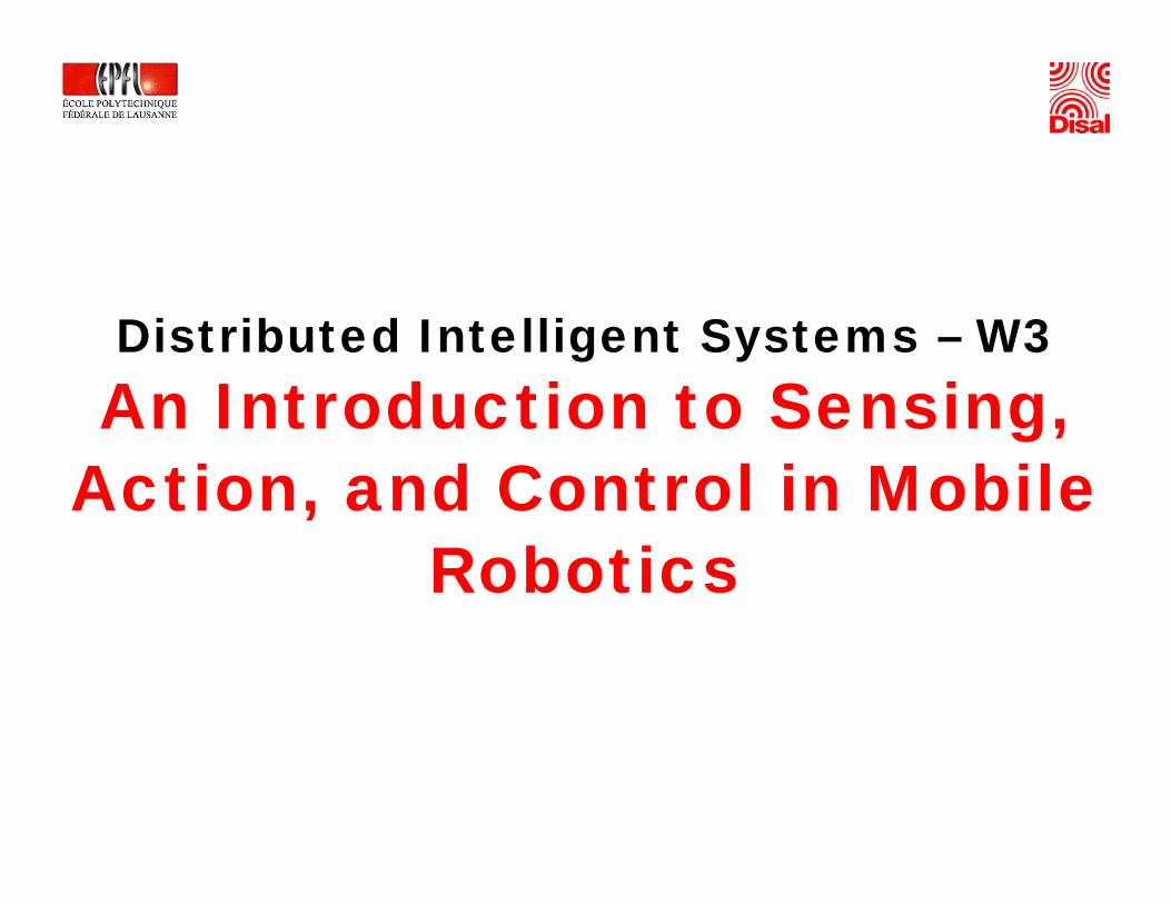
Outline• General concepts
– AutonomyAutonomy– Perception-to-action loop– Sensing, actuating, computing
• e-puck– Basic features
HW hit t– HW architecture• Main example of reactive control
architecturesarchitectures– Proximal architectures– Distal architectures
General Concepts and General Concepts and Principles for Mobile
Robotics
AutonomyAutonomy
• Different levels/degrees of autonomyDifferent levels/degrees of autonomy– Energetic level– Sensory motor and computational levelSensory, motor, and computational level– Decisional level
• Needed degree of autonomy depends on task/environment in which the unit has to operateE i t l di t bilit i i l b t• Environmental unpredictability is crucial: robot manipulator vs. mobile robot vs. sensor node
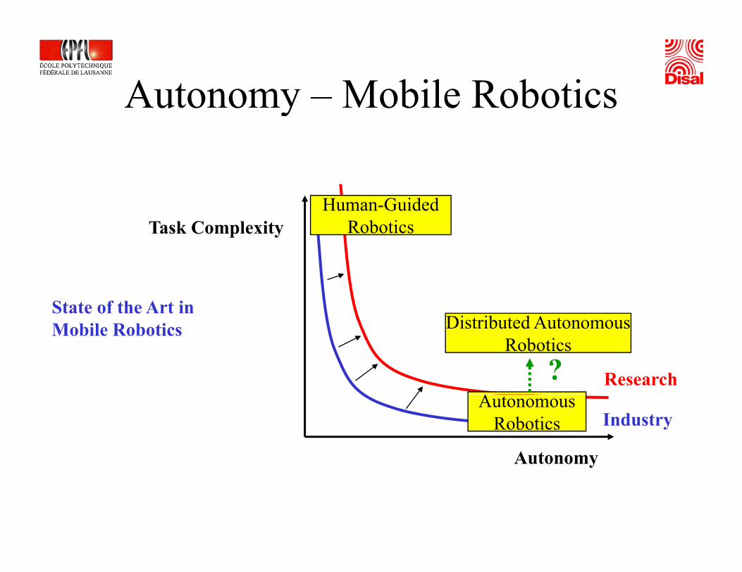
Autonomy – Mobile RoboticsAutonomy Mobile Robotics
Task ComplexityHuman-Guided
Robotics
State of the Art in Distributed AutonomousMobile Robotics
Research
Distributed AutonomousRobotics
?
Autonomy
IndustryAutonomous
Robotics
y
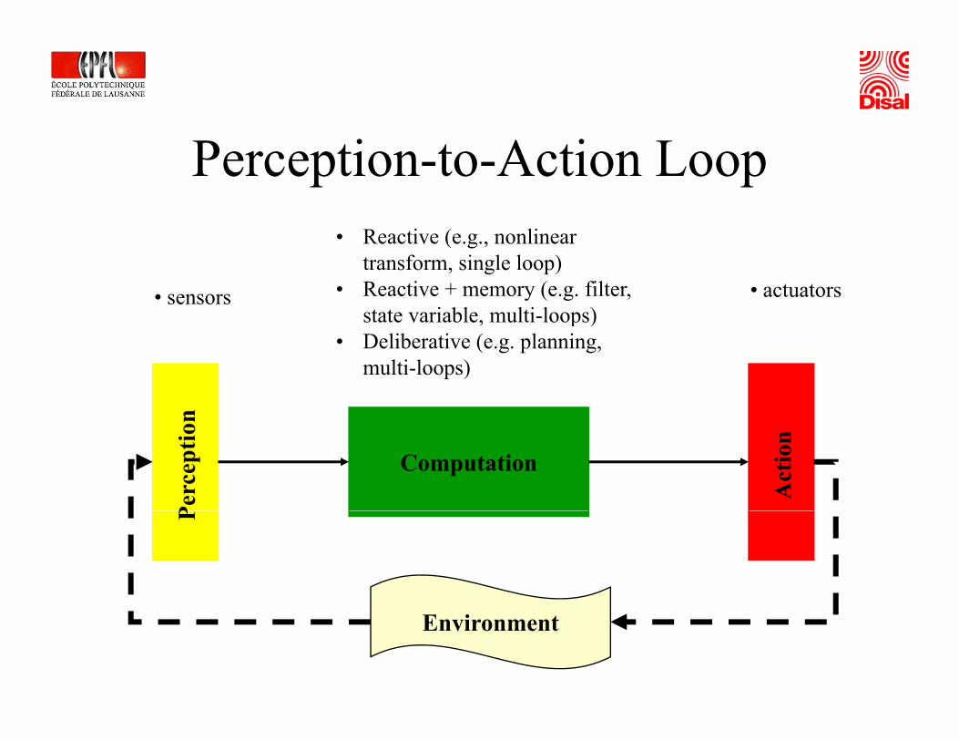
Perception-to-Action LoopR i ( li• Reactive (e.g., nonlinear transform, single loop)
• Reactive + memory (e.g. filter, state variable, multi-loops)
• sensors • actuators
n
, p )• Deliberative (e.g. planning,
multi-loops)
Computation
Perc
eptio
n
Act
ion
P
Environment
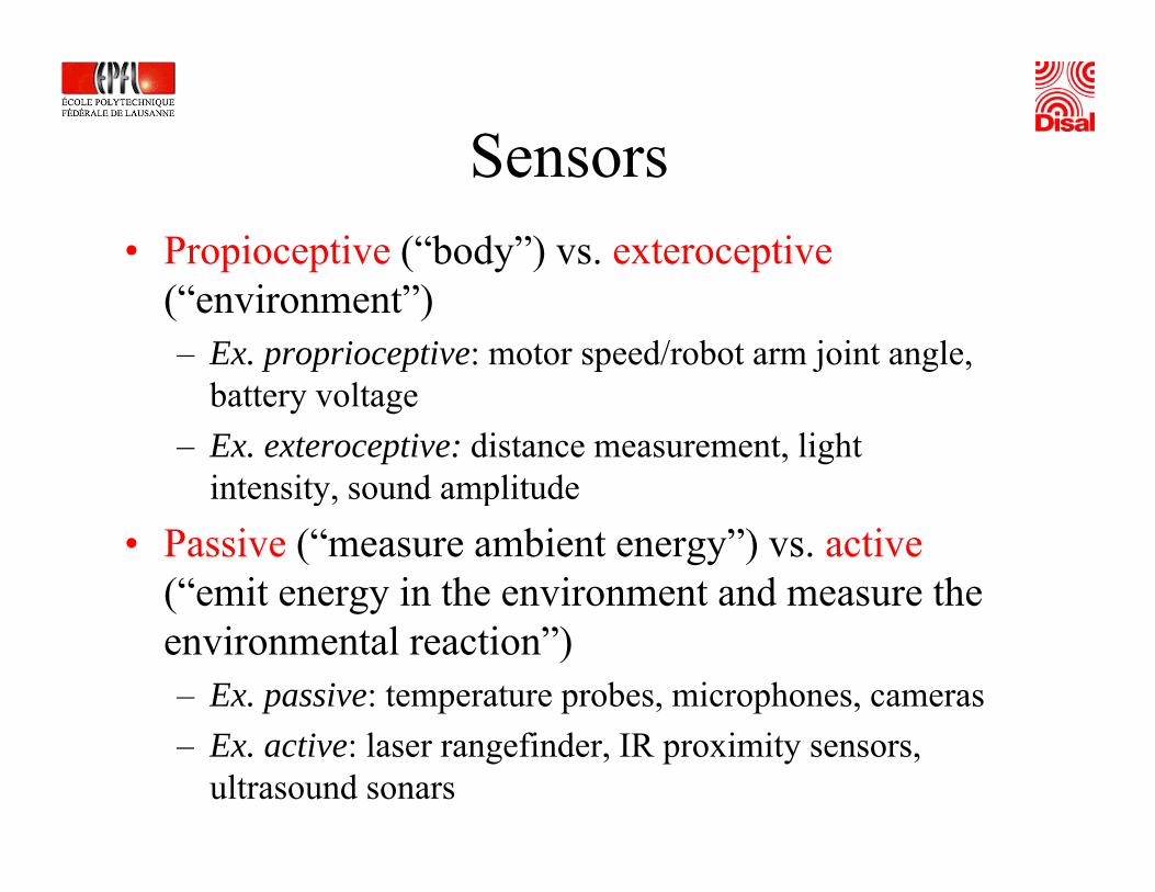
SensorsSensors• Propioceptive (“body”) vs. exteroceptive
(“environment”)– Ex. proprioceptive: motor speed/robot arm joint angle,
b tt ltbattery voltage– Ex. exteroceptive: distance measurement, light
intensity, sound amplitudey, p
• Passive (“measure ambient energy”) vs. active(“emit energy in the environment and measure the environmental reaction”)– Ex. passive: temperature probes, microphones, cameras– Ex. active: laser rangefinder, IR proximity sensors,
ultrasound sonars
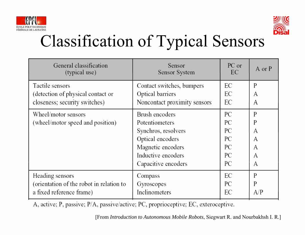
Classification of Typical SensorsClassification of Typical Sensors
[From Introduction to Autonomous Mobile Robots, Siegwart R. and Nourbakhsh I. R.]
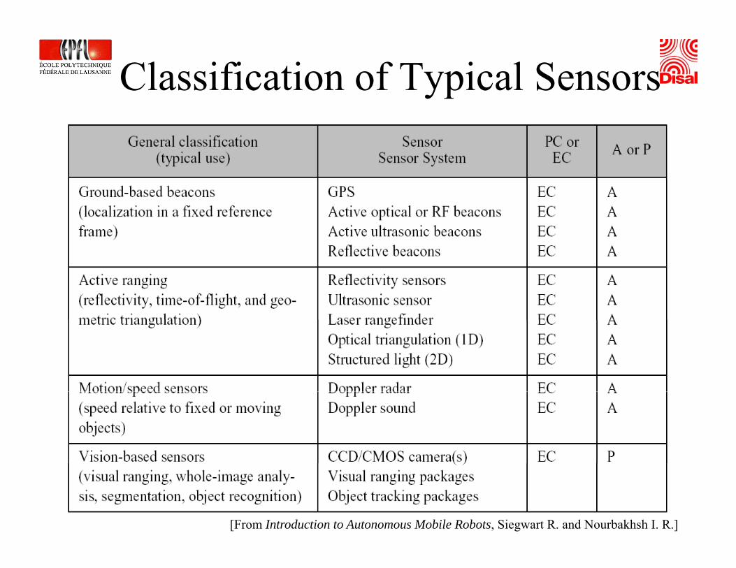
Classification of Typical Sensors
[From Introduction to Autonomous Mobile Robots, Siegwart R. and Nourbakhsh I. R.]
Action - Actuators
• For different purposes: locomotion, control a part of the body (e.g. arm), heating, sound p y ( g ), g,producing, etc.
• Examples of electrical-to-mechanicalExamples of electrical to mechanical actuators: DC motors, stepper motors, servos loudspeakers etcservos, loudspeakers, etc.
ComputationComputation• Usually microcontroller-based; memory y y
internal and potentially external to the microcontroller
• “Discretization” (analog-to-digital for values, continuous-to-discrete for time) andvalues, continuous to discrete for time) and “continuization” (digital-to-analog for values, discrete-to-continuous for time)values, discrete to continuous for time)
• Different types of control architectures: e.g., reactive (‘reflex based”) vs deliberativereactive ( reflex-based ) vs. deliberative (“planning”)
Sensor Performance
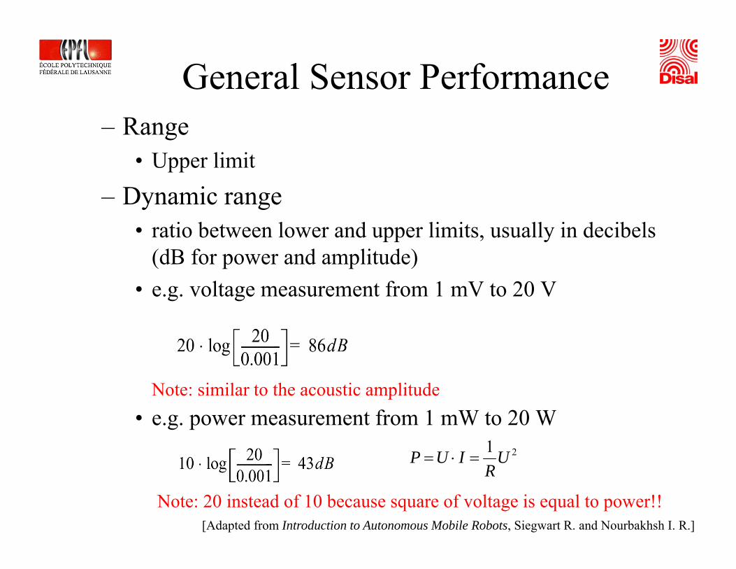
General Sensor Performance– Range
• Upper limit
– Dynamic range• ratio between lower and upper limits, usually in decibels
(d f d li d )(dB for power and amplitude)• e.g. voltage measurement from 1 mV to 20 V
Note: similar to the acoustic amplitude• e.g. power measurement from 1 mW to 20 W
21 UIUP =⋅=
Note: similar to the acoustic amplitude
R
Note: 20 instead of 10 because square of voltage is equal to power!![Adapted from Introduction to Autonomous Mobile Robots, Siegwart R. and Nourbakhsh I. R.]
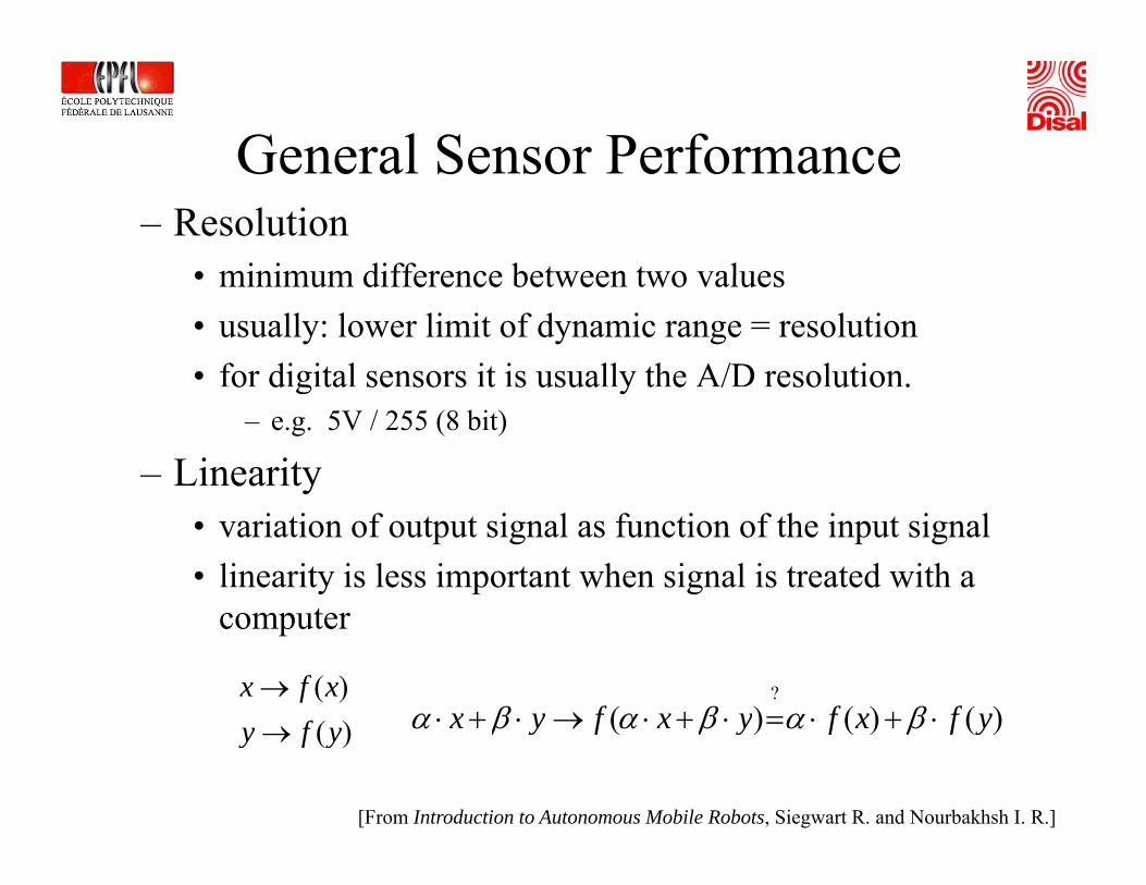
General Sensor Performance– Resolution
• minimum difference between two values
General Sensor Performance
• minimum difference between two values• usually: lower limit of dynamic range = resolution• for digital sensors it is usually the A/D resolution.o d g ta se so s t s usua y t e / eso ut o .
– e.g. 5V / 255 (8 bit)
– Linearity• variation of output signal as function of the input signal• linearity is less important when signal is treated with a
tcomputer
)()(
fxfx →
)()()(?
yfxfyxfyx ⋅+⋅=⋅+⋅→⋅+⋅ βαβαβα)(yfy → )()()( yfxfyxfyx +=+→+ βαβαβα
[From Introduction to Autonomous Mobile Robots, Siegwart R. and Nourbakhsh I. R.]
General Sensor Performance
– Bandwidth or Frequency
General Sensor Performance
• the speed with which a sensor can provide a stream of readings
ll th i li it d di th• usually there is an upper limit depending on the sensor and the sampling rate
• lower limit is also possible, e.g. acceleration sensorp , g• frequency response: phase (delay) of the signal and
amplitude might be influenced
[Adapted from Introduction to Autonomous Mobile Robots, Siegwart R. and Nourbakhsh I. R.]
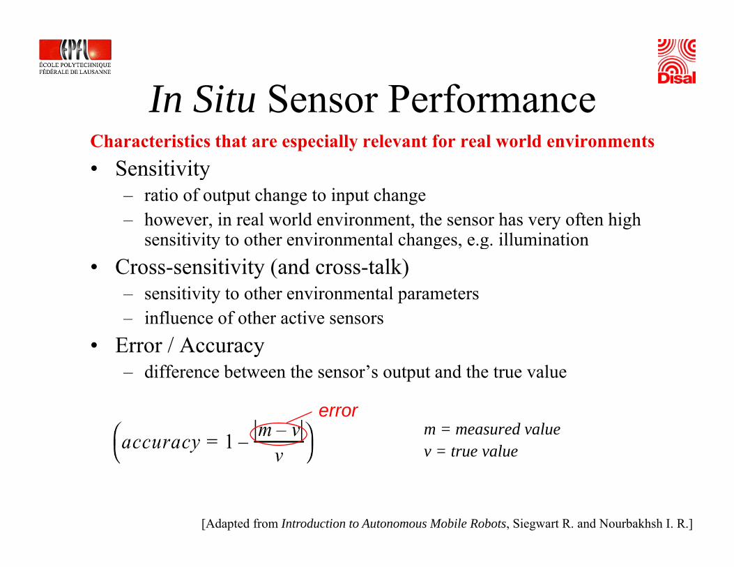
In Situ Sensor PerformanceIn Situ Sensor PerformanceCharacteristics that are especially relevant for real world environments• Sensitivityy
– ratio of output change to input change– however, in real world environment, the sensor has very often high
sensitivity to other environmental changes, e.g. illuminationy g , g• Cross-sensitivity (and cross-talk)
– sensitivity to other environmental parameters– influence of other active sensors– influence of other active sensors
• Error / Accuracy– difference between the sensor’s output and the true value
m = measured valuev = true value
error
[Adapted from Introduction to Autonomous Mobile Robots, Siegwart R. and Nourbakhsh I. R.]
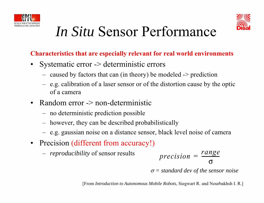
In Situ Sensor Performance Characteristics that are especially relevant for real world environments
• Systematic error > deterministic errors• Systematic error -> deterministic errors– caused by factors that can (in theory) be modeled -> prediction– e.g. calibration of a laser sensor or of the distortion cause by the optic
of a camera
• Random error -> non-deterministic– no deterministic prediction possibleno deterministic prediction possible– however, they can be described probabilistically – e.g. gaussian noise on a distance sensor, black level noise of camera
i i (diff f )• Precision (different from accuracy!)– reproducibility of sensor results
[From Introduction to Autonomous Mobile Robots, Siegwart R. and Nourbakhsh I. R.]
σ = standard dev of the sensor noise
k A Ed ti l e-puck: An Educational Robotic ToolRobotic Tool
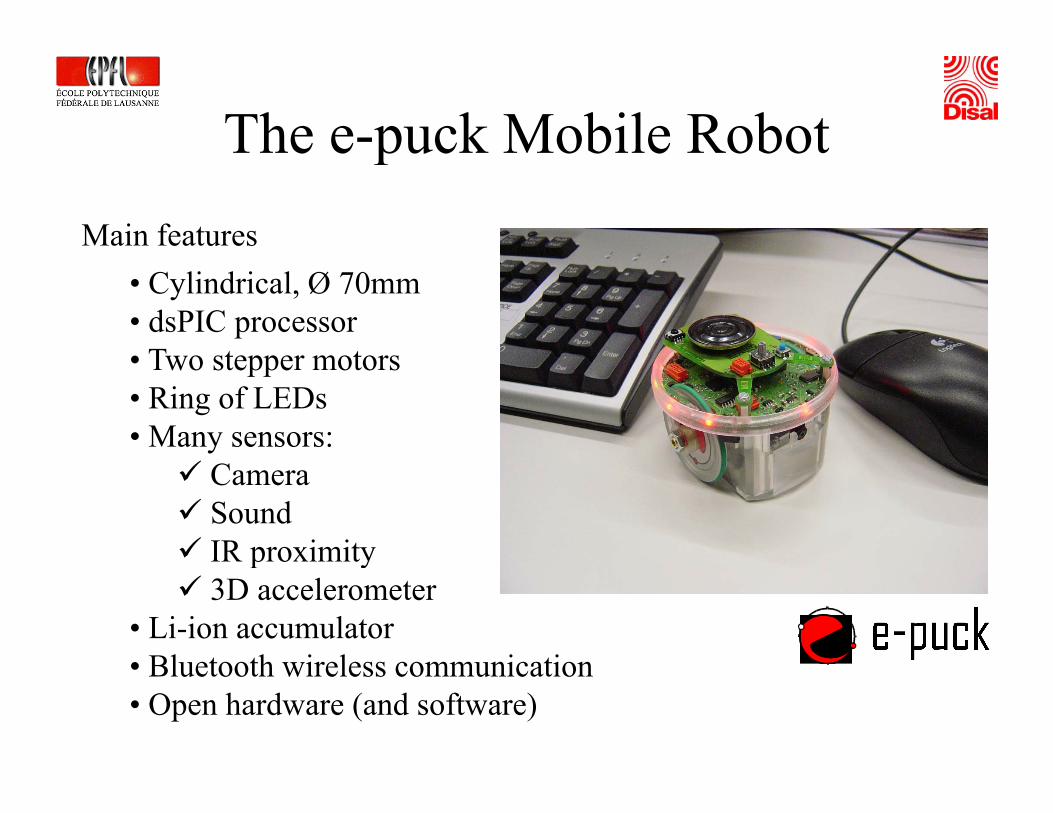
The e-puck Mobile RobotMain features
The e puck Mobile Robot
• Cylindrical, Ø 70mm• dsPIC processor
T o stepper motors• Two stepper motors• Ring of LEDs• Many sensors:
CameraSoundIR proximityIR proximity3D accelerometer
• Li-ion accumulator• Bluetooth wireless communication• Bluetooth wireless communication• Open hardware (and software)
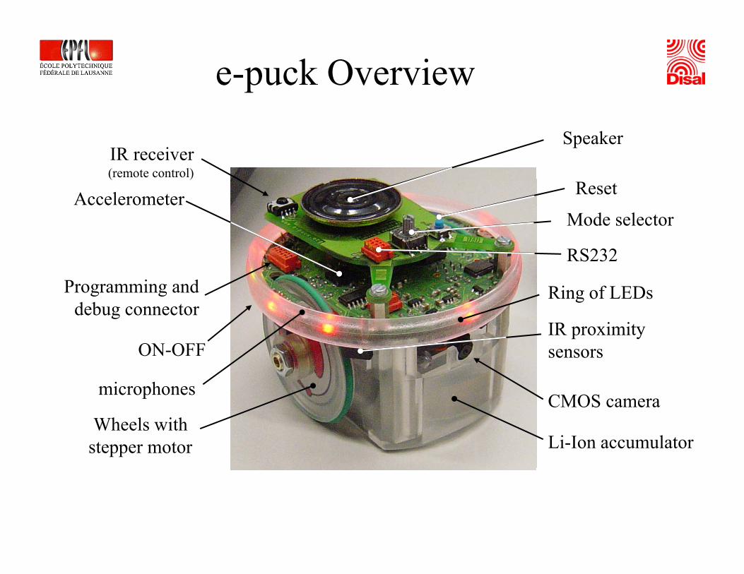
e-puck Overview
IR receiver(remote control)
Speaker
RS232
Accelerometer( )
Mode selector
Reset
RS232
Ring of LEDs
IR i i
Programming anddebug connector
ON-OFFIR proximity sensors
CMOSmicrophones
Wheels with stepper motor Li-Ion accumulator
CMOS camerap
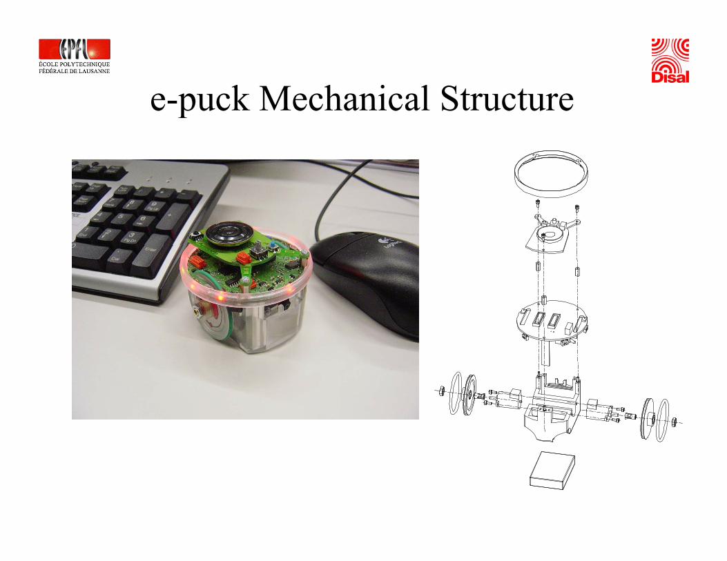
e-puck Mechanical Structuree puck Mechanical Structure
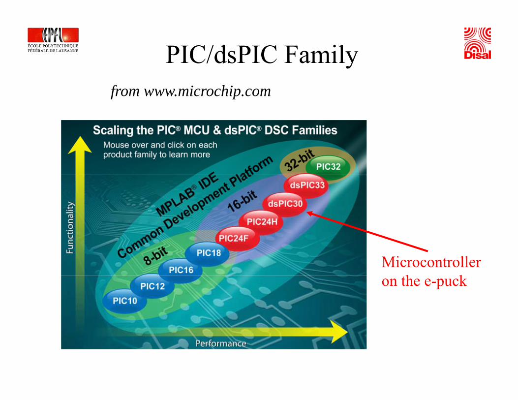
PIC/dsPIC Familyfrom www.microchip.com
Microcontroller h kon the e-puck
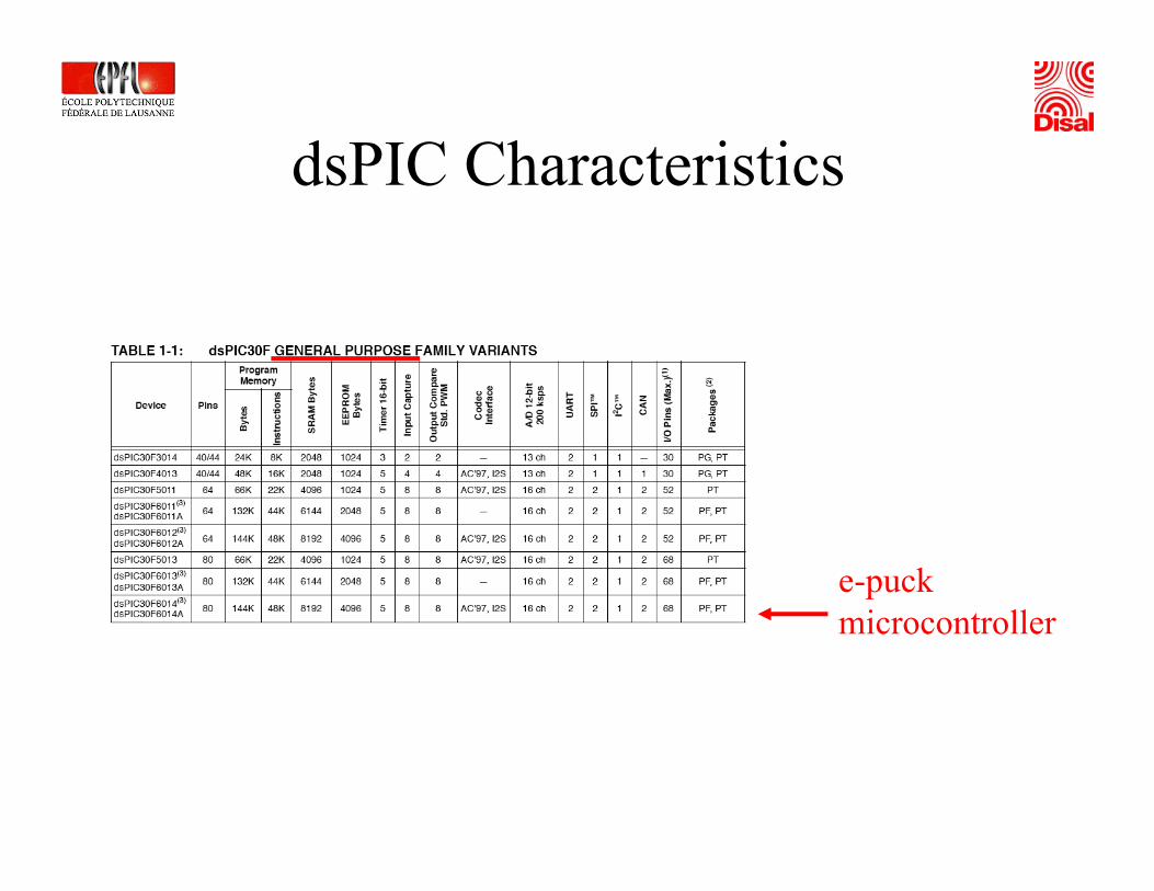
dsPIC CharacteristicsdsPIC Characteristics
e-pucki t llmicrocontroller
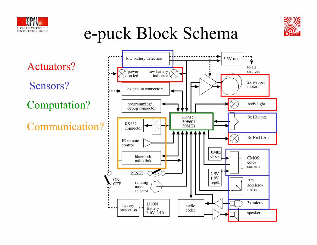
e-puck Block Schema
Actuators?
Sensors?
Computation?Computation?
Communication?
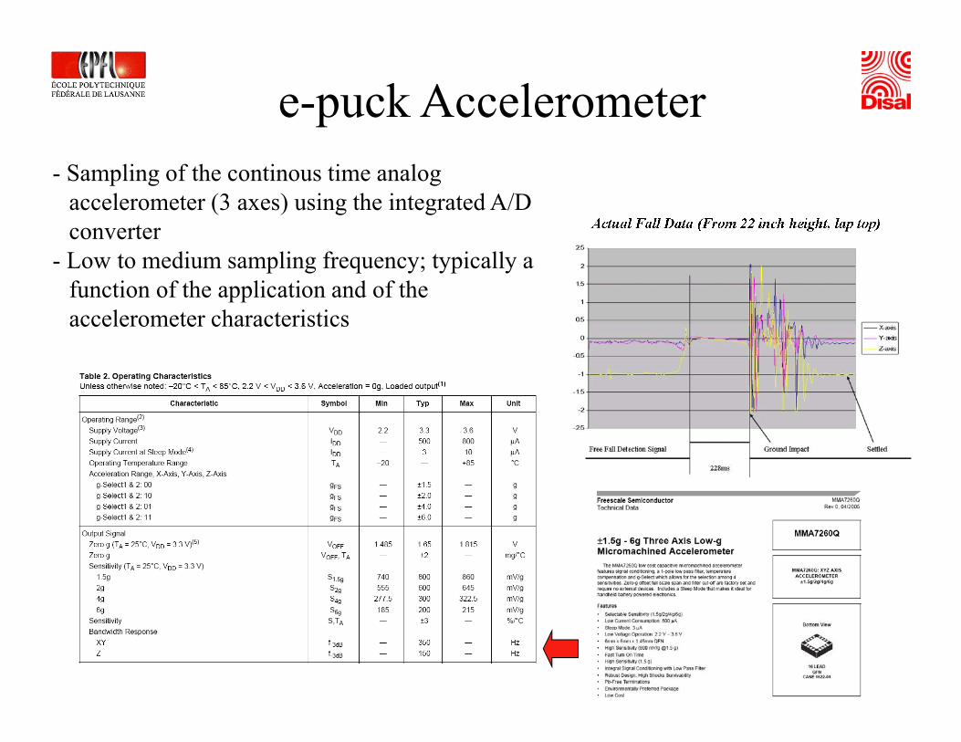
e-puck Accelerometer- Sampling of the continous time analog
accelerometer (3 axes) using the integrated A/D converterconverter
- Low to medium sampling frequency; typically a function of the application and of the accelerometer characteristicsaccelerometer characteristics
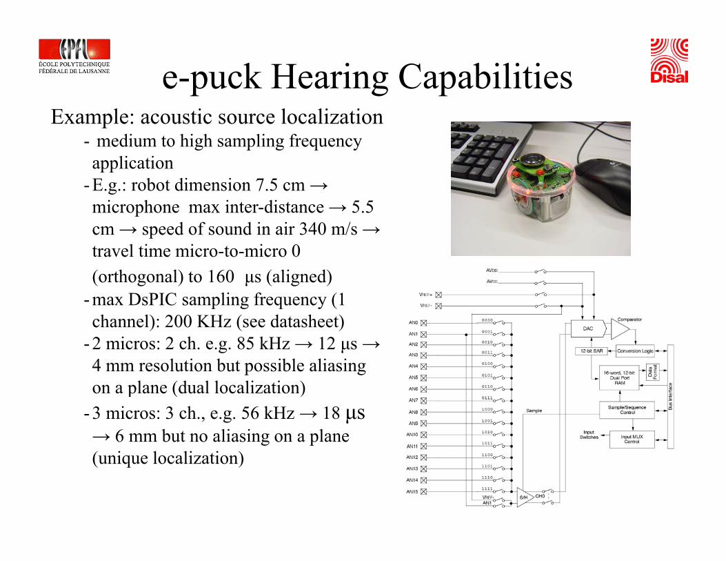
e-puck Hearing CapabilitiesExample: acoustic source localization
- medium to high sampling frequency application
- E.g.: robot dimension 7.5 cm → microphone max inter-distance → 5.5 cm → speed of sound in air 340 m/s →
l i i i 0travel time micro-to-micro 0 (orthogonal) to 160 μs (aligned)
- max DsPIC sampling frequency (1 h l) 200 KH ( d h )channel): 200 KHz (see datasheet)
- 2 micros: 2 ch. e.g. 85 kHz → 12 μs →4 mm resolution but possible aliasing on a plane (dual localization)on a plane (dual localization)
- 3 micros: 3 ch., e.g. 56 kHz → 18 μs→ 6 mm but no aliasing on a plane (unique localization)(unique localization)
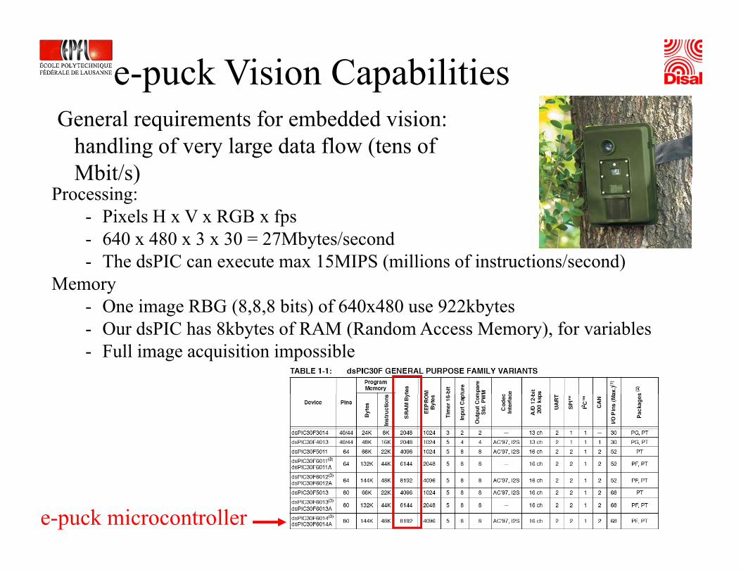
e-puck Vision Capabilities General requirements for embedded vision:
handling of very large data flow (tens of Mbit/s)
Processing:- Pixels H x V x RGB x fps- 640 x 480 x 3 x 30 = 27Mbytes/second
Mbit/s)
- The dsPIC can execute max 15MIPS (millions of instructions/second)Memory
- One image RBG (8,8,8 bits) of 640x480 use 922kbytesO d C h 8kb f A ( d A ) f i bl- Our dsPIC has 8kbytes of RAM (Random Access Memory), for variables
- Full image acquisition impossible
e-puck microcontroller
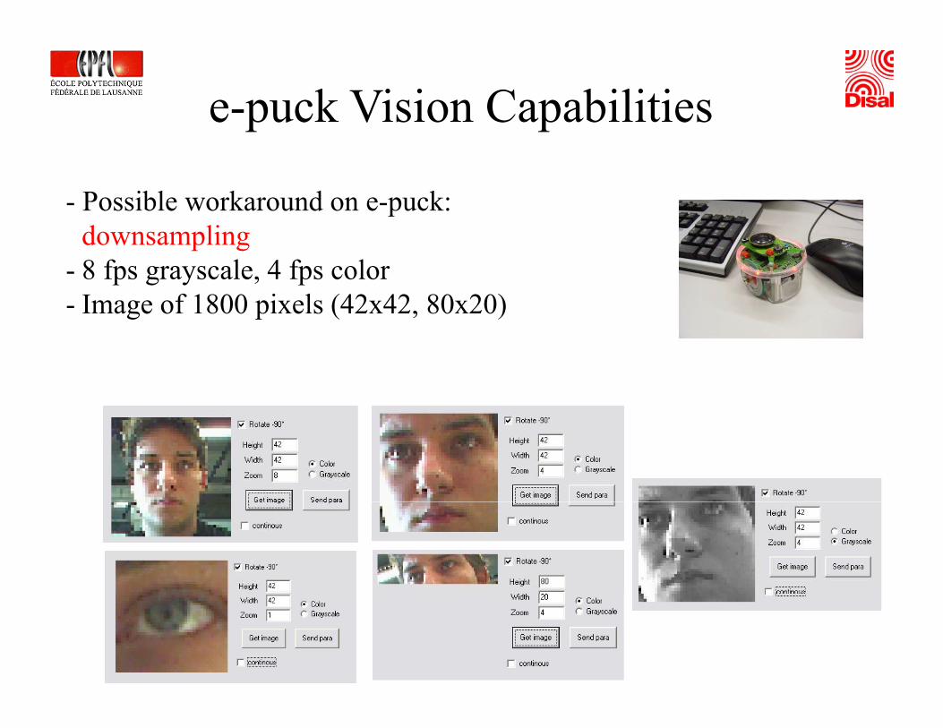
e-puck Vision Capabilities
- Possible workaround on e-puck: d lidownsampling
- 8 fps grayscale, 4 fps color- Image of 1800 pixels (42x42, 80x20)g p ( )
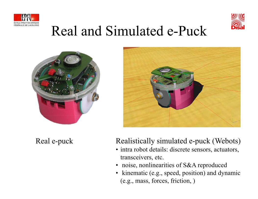
Real and Simulated e-Puck
Real e-puck Realistically simulated e-puck (Webots)• intra robot details: discrete sensors, actuators,
transceivers, etc.• noise, nonlinearities of S&A reproduced• kinematic (e.g., speed, position) and dynamic
(e.g., mass, forces, friction, )
E l f R ti Examples of Reactive Control ArchitecturesControl Architectures
Reactive Architectures:Reactive Architectures: Proximal vs. Distal in Theory
• Proximal: l d– close to sensor and actuators
– very simple linear/nonlinear operators on crude d tdata
– high flexibility in shaping the behavioriffi l i i “h id d”– Difficult to engineer in a “human-guided” way;
machine-learning usually perform better
Reactive Architectures:Reactive Architectures: Proximal vs. Distal in Theory
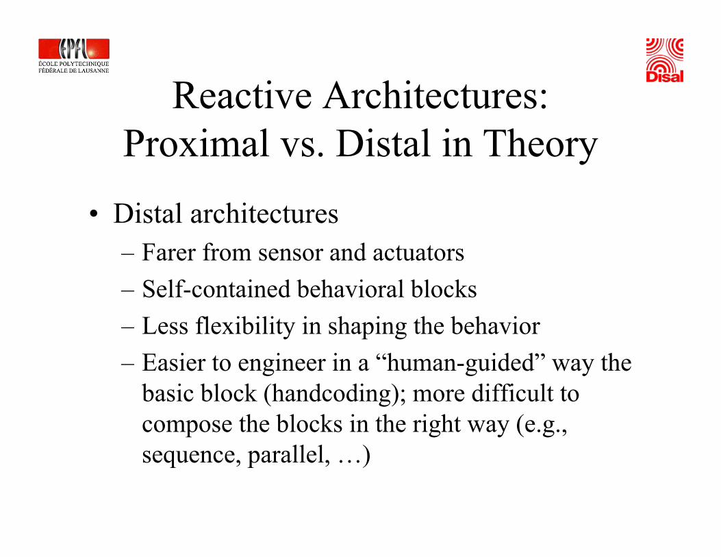
• Distal architectures F f d– Farer from sensor and actuators
– Self-contained behavioral blocks – Less flexibility in shaping the behavior– Easier to engineer in a “human-guided” way the
b i bl k (h d di ) diffi lbasic block (handcoding); more difficult to compose the blocks in the right way (e.g., sequence parallel )sequence, parallel, …)
Reactive Architectures:Reactive Architectures: Proximal vs. Distal in Practice
• A whole blend!• Five “classical” examples of reactive p
control architecture for solving the same problem: obstacle avoidance.
• Two proximal: Braitenberg and Artificial Neural Network
• Three distal: rule-based and two behavior-based (Subsumption and Motor Schema)
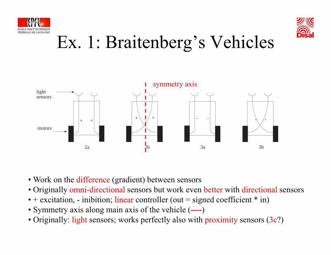
Ex. 1: Braitenberg’s VehiclesEx. 1: Braitenberg s Vehicles
lightsensors
symmetry axis
- - --
motors
++++
2a 2b 3a 3b
• Work on the difference (gradient) between sensors• Originally omni-directional sensors but work even better with directional sensors• + excitation, - inibition; linear controller (out = signed coefficient * in)
S t i l i i f th hi l ( )• Symmetry axis along main axis of the vehicle (----)• Originally: light sensors; works perfectly also with proximity sensors (3c?)
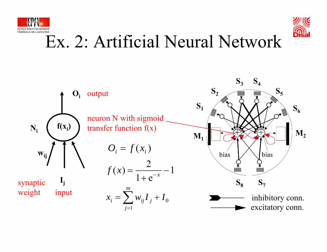
Ex. 2: Artificial Neural NetworkEx. 2: Artificial Neural Network
S Soutput
S1
S2
S3 S4S5
S6
Oi
f(xi)Ni
neuron N with sigmoidtransfer function f(x)
1 S6
M1M2
wij
12)( −=xf
)( ii xfO =
Ije1
)(+ −xf
synaptic weight input
S7S8
∑ +=m
jiji IIwx 0 inhibitory conn.it t=j 1 excitatory conn.
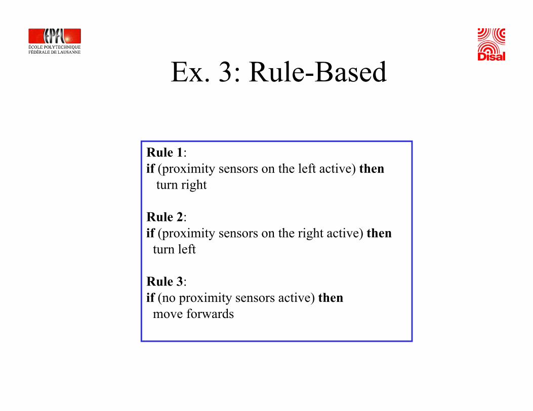
Ex 3: Rule-BasedEx. 3: Rule Based
Rule 1:if (proximity sensors on the left active) then
i hturn right
Rule 2:if (proximity sensors on the right active) thenif (proximity sensors on the right active) thenturn left
Rule 3:Rule 3:if (no proximity sensors active) thenmove forwards
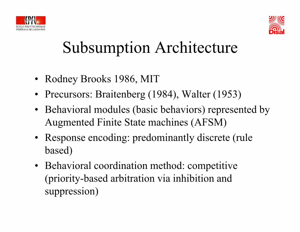
S b ti A hit tSubsumption Architecture
• Rodney Brooks 1986, MIT• Precursors: Braitenberg (1984), Walter (1953)• Behavioral modules (basic behaviors) represented by
Augmented Finite State machines (AFSM)• Response encoding: predominantly discrete (rule
based)• Behavioral coordination method: competitive
(priority-based arbitration via inhibition and i )suppression)
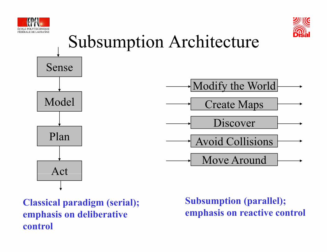
Subsumption ArchitectureSubsumption ArchitectureSense
ModelModify the World
Create Maps
Plan
pDiscover
Avoid Collisions
Act
Avoid CollisionsMove Around
Act
Classical paradigm (serial); Subsumption (parallel); Classical paradigm (serial);emphasis on deliberativecontrol
p (p );emphasis on reactive control
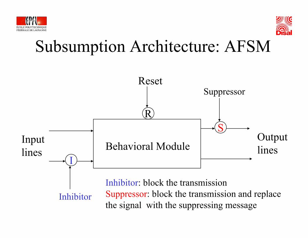
S bs mption Architect re: AFSMSubsumption Architecture: AFSM
ResetSuppressor
RS
O t tBehavioral Module
I
Inputlines
Outputlines
I hibitInhibitor: block the transmissionSuppressor: block the transmission and replaceInhibitor Suppressor: block the transmission and replacethe signal with the suppressing message
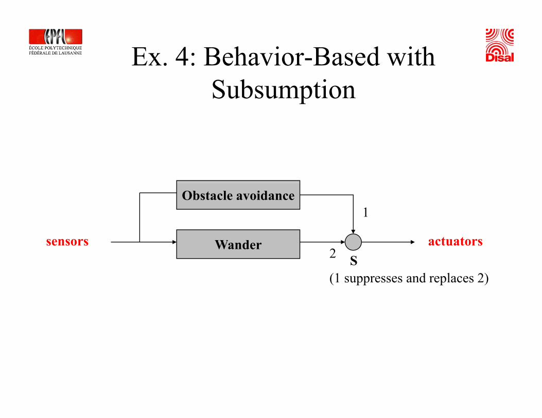
Ex. 4: Behavior-Based with Subsumption
Obstacle avoidance1
WanderS
(1 suppresses and replaces 2)
actuatorssensors2
Evaluation of Subsumption
+ Support for parallelism: each behavioral layer can run independently and asynchronously (including different loop time)loop time)
+ Fast execution time possible
- Coordination mechanisms restrictive (“black or white”)- Limited support for modularity (upper layers design cannot
be independent from lower layers).
Motor SchemasMotor Schemas
R ld A ki 1987 G i T h• Ronald Arkin 1987, Georgia Tech• Precursors: Arbib (1981), Khatib (1985)• Parametrized behavioral libraries
(schemas)( )• Response encoding: continuous using
potential field analogpotential field analog• Behavioral coordination method:
cooperative via vector summation andcooperative via vector summation and normalization
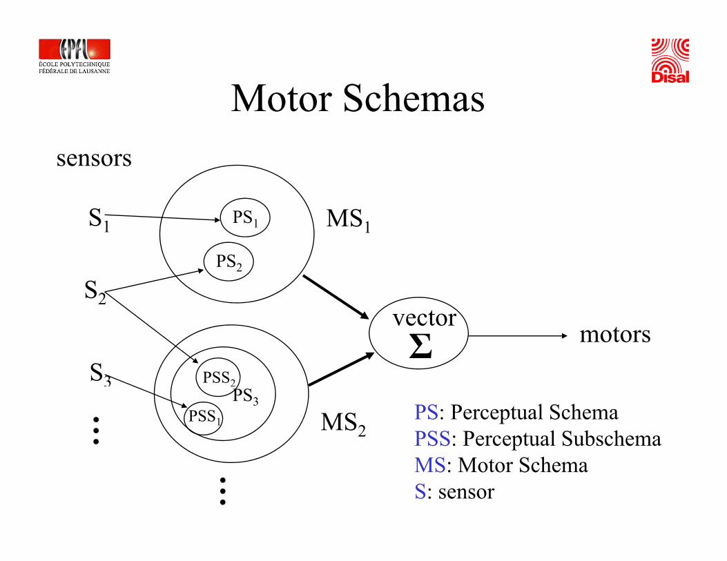
Motor SchemasMotor Schemassensors
MS1PS1S1
vector
PS2
S2
Σvector motors
PSS2S3
MS2
PS3PSS1
… PS: Perceptual SchemaPSS: Perceptual SubschemaMS M S h… MS: Motor SchemaS: sensor
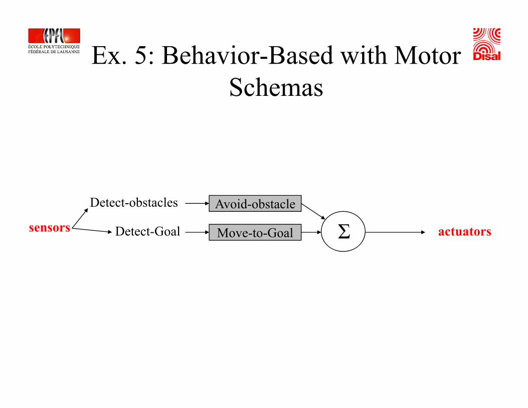
Ex. 5: Behavior-Based with Motor Schemas
Avoid-obstacle
ΣDetect-obstacles
M t G lDetect Goal actuatorssensors ΣMove-to-GoalDetect-Goal actuatorssensors
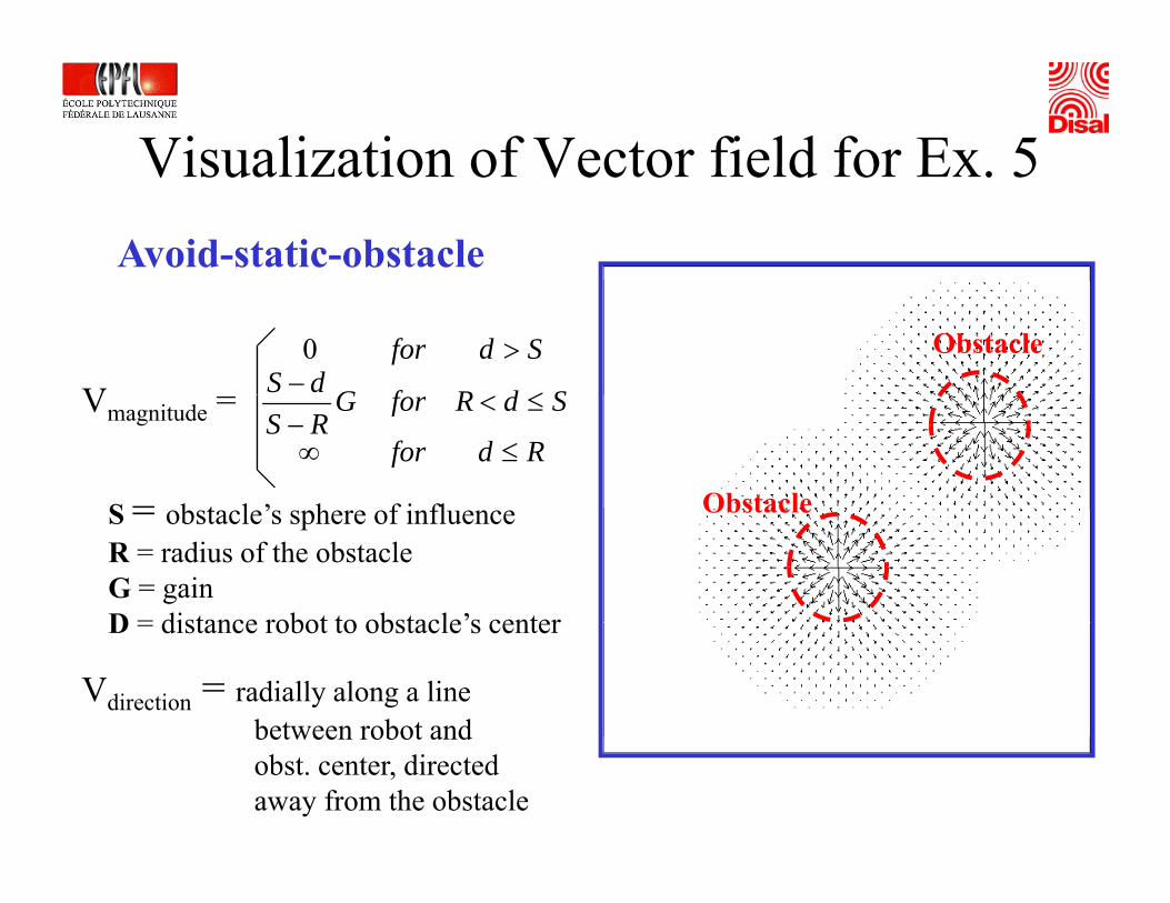
Visualization of Vector field for Ex 5Visualization of Vector field for Ex. 5Avoid-static-obstacle
Obstacle
V SdRfGdSSdfor
≤−
>0
Obstacle
Vmagnitude =Rdfor
SdRforGRS
≤∞
≤<−
S = b t l ’ h f i fl ObstacleS = obstacle’s sphere of influenceR = radius of the obstacleG = gainD = distance robot to obstacle’s center
Vdirection = radially along a line between robot and
D = distance robot to obstacle s center
between robot and obst. center, directed away from the obstacle
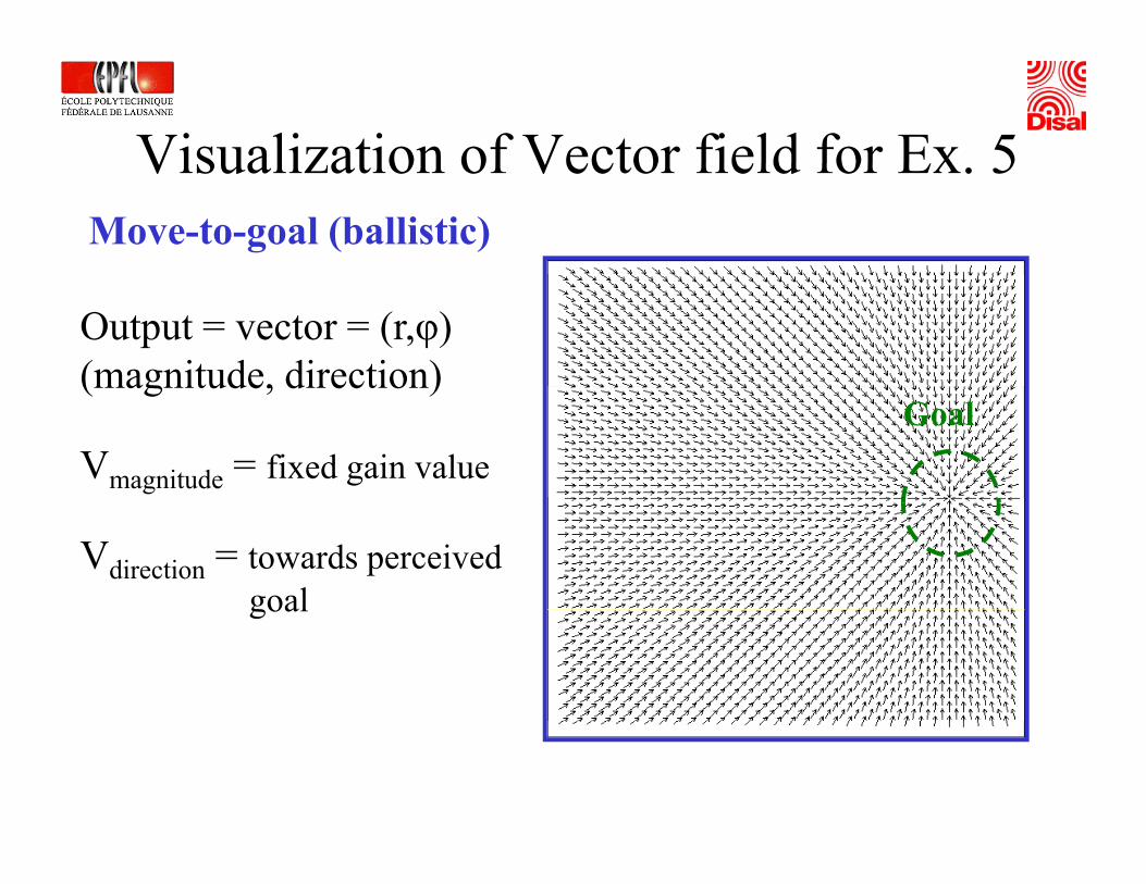
Visualization of Vector field for Ex 5Move-to-goal (ballistic)
Visualization of Vector field for Ex. 5
Output = vector = (r,φ)(magnitude, direction)
Goal(magnitude, direction)
Vmagnitude = fixed gain value
Vdirection = towards perceived goalgoal
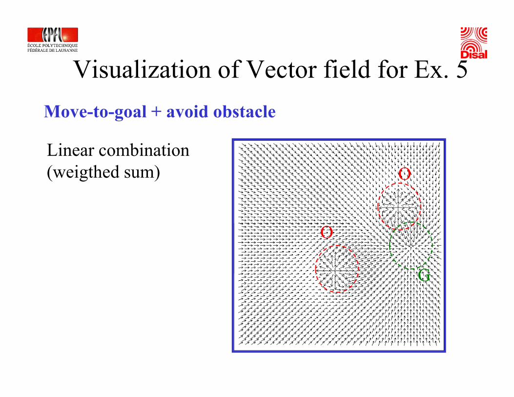
Visualization of Vector field for Ex 5Move-to-goal + avoid obstacle
Visualization of Vector field for Ex. 5
OLinear combination(weigthed sum) O(weigthed sum)
G
O
G
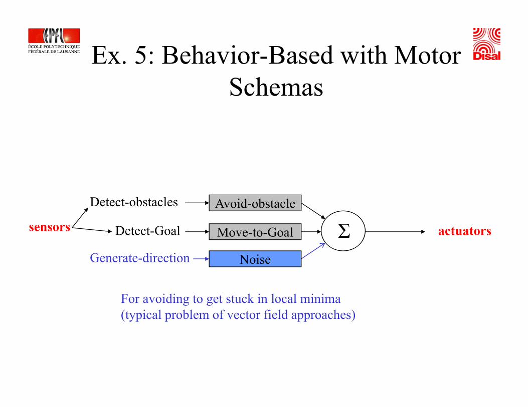
Ex. 5: Behavior-Based with Motor Schemas
Avoid-obstacle
ΣDetect-obstacles
M t G lDetect Goal actuatorssensors ΣMove-to-GoalDetect-Goal actuatorssensors
NoiseGenerate-direction
For avoiding to get stuck in local minima (typical problem of vector field approaches)
Evaluation of Motor Schemas
+ Support for parallelism: motor schemas are naturally parallelizable
+ Fi d b h i l bl di ibl+ Fine-tuned behavioral blending possible
- Robustness > well known problems of potential field- Robustness -> well-known problems of potential field approach -> extra introduction of noise (not clear method for exploiting that generated by sensors, …)
- Slow and computationally expensive sometimes
Evaluation of both Architectures in Practice
• In pratice (my expertise) you tend to mix both and even moreeven more …
• The way to combine basic behavior (collaborative and/or competitive) depends from how you p ) p ydeveloped the basic behaviors (or motor schemas), reaction time required, on-board computational capabilitiescapabilities, …

Conclusion
Take Home Messages• Perception-to-action loop is key in robotics, several
sensor and actuator modalitiesK t i f l ifi ti t ti• Key categories for sensor classification are exteroceptivevs. propioceptive and active vs. passive
• Experimental work can be carried out with real and prealistically simulated robots
• A given behavior can be obtained with different control architecturesarchitectures
• Control architectures can be roughly classified in proximal and distal architectures
• Braitenberg vehicles and artificial neural networks are two typical examples of proximal architecture, motor schema and subsumption architecture are typicalschema and subsumption architecture are typical example of distal architecture
Additional Literature – Week 3Books• Braitenberg V., “Vehicles: Experiments inBraitenberg V., Vehicles: Experiments in
Synthetic Psychology”, MIT Press, 1986.• Siegwart R., Nourbakhsh I. R., and
Scaramuzza D., “Introduction to Autonomous Mobile Robots”, 2nd edition, MIT Press, 2011. A ki R C “B h i B d R b ti ” MIT• Arkin R. C., “Behavior-Based Robotics”. MIT Press, 1998.
• Everett H R “Sensors for Mobile Robots• Everett, H. R., Sensors for Mobile Robots, Theory and Application”, A. K. Peters, Ltd., 1995
Recommended