Working Paper 81-2
DISCOUNT WINDOW BORROWING, MONETARY POLICY,
AND THE POST-OCTOBER 6, 1979 FEDERAL
RESERVE OPERATING PROCEDURE*
Marvin Goodfriend
Federal Reserve Bank of Richmond
Revised September 1, 1981
*The author is Research Officer and Economist at the Federal Reserve Bank of Richmond. Discussions with Tim Cook have been particularly valuable. Thanks are also due to John Boschen, Bob Ring, Rich Lang, Ben McCallum, John McDermott, Tom Mead, and Jerome Stein. The views here are solely those of the author and do not necessarily reflect the views of the Federal Reserve Bank of Richmond or the Federal Reserve System.

Introduction
This paper is intended to be an analysis of discount
window borrowing as it relates to 'more general issues of monetary
control. The topic deserves a new look because of the central
role of discount window borrowing under the post-October 6, 1979
"reserve targeting" operating strategy.
The analytical core of the paper is the derivation of
a demand for borrowing function based on profit-maximizing bank
behavior. It is shown that a basic feature of the nonprice
rationing mechanism at the discount window causes the banks
to solve a dynamic optimization problem in deciding on optimal
current discount window borrowing. The solution of this problem
for the structure of the borrowing demand function has
implications for the conduct of monetary policy. These are
brought out in the latter sections of the paper.
Nonprice Rationing at the Discount Window
If there were no nonprice rationing at the discount
window, the Federal funds rate would never rise above the
discount rate, because a bank would never pay more for reserves
than it would have to pay at the discount window. Since 1965,
the Federal funds rate has, on numerous occasions, risen above
the discount rate. On two occasions it has remained above the
discount rate for roughly two years running. This indicates
-l-

.-2-
that an effective form of nonprice rationing is xbeing administered
at the discount window.
The basis for this nonprice rationing is spelled out
in Regulation A. The condition under which a bank is entitled
to "adjustment credit" at the discount window is stated in
Regulation A as follows:
Federal Reserve credit is available on a short-term basis to a depository institution under such rules as may be prescribed to assist the institution, to the extent appropriate, in meeting temporary requirements for funds, or to cushion more persistent outflows of funds pending an orderly adjustment of the institution's assets and liabilities.'
The sense of this statement of privilege is that
appropriate borrowing should be temporary. The intention is
clearly that discount officers and committees should use
duration as a fair objective measure of appropria.teness, with
appropriateness negatively related to duration. This intention
is also clearly expressed in the Report of the System Committee
on the Discount and Discount Rate Mechanism (1954), where it is
suggested that "the duration of borrowing [is] to be used to
establish a rebuttable presumption that borrowing [is] for an 2
inappropriate purpose."
Reserve Banks have set up rules for administering their
discount windows based on duration as a measure of appropriateness.
A common feature of these rules is a set of restrictions on the
number of weeks a bank can be "in the window" during a specified
period. Such "frequency" restrictions exist for 13-, 26-, and
52-week periods.3 In general, the rules seem to be designed to

-3-
apply progressively heavier pressure to banks the more lengthy a
given "stay in the window."
From the point of view.of modeling borrowing behavior,
there are many unsatisfactory features of the nonprice rationing
mechanism in force at the Reserve Banks. The nonprice costs imposed
on banks are difficult to identify. -The frequency guidelines are
difficult to incorporate in an operational empirical model of the
demand for borrowing. And the lack of uniformity in.discount
window administration across Reserve Banks contributes to the
difficulty in modeling aggregate borrowing. However, these problems
are ignored in this paper in order to fully concentrate on the
effect of "progressive pressure" in influencing the structure of
the bank borrowing function.
4 A Model of the Bank Borrowing Decision
Major aspects of the bank borrowing decision are
described in this section. Banks are assumed to behave rationally
and to maximize profits. Because of the mechanism of nonprice
rationing at the discount window, banks turn out to care about
the past and future in deciding how much to currently borrow.
In other words, they face a "dynamic optimization problem." In
the following two sections, a simple formal solution to this
optimization problem is derived and some characteristics of the
bank borrowing function are discussed.
Even a simple version of this dynamic optimization
problem is fairly complex. Consequently, a simple form of
discount window nonprice rationing mechanism is assumed for

-4-
this disc'ussion. First, the marginal perceived effective cost
of borrowing is assumed to rise with borrowing in the current
period. Second, given the current level of borrowing, the marginal
perceived effective cost of borrowing'is assumed to be positively
related to the level of borrowing last period.
A simple cost of borrowing function that embodies the
two essential features of the nonprice rationing mechanism
described above may be written
(1) Ct cO = klBtel + l)-+(Bt + 1) 2 - 11 + dtBt
where d t = the period t discount rate
co’ cl ’ 0, Btr BtBl 1 0
This cost function is graphed in Figure 1 for a given current
discount rate and lagged level of borrowing. The functional form
has a number of reasonable characteristics. First, the cost is
zero when current borrowing, Bt, is zero, i.e., the function passes
through the origin. Second, the marginal cost of current borrowing
is positive and rises with the level of current borrowing, i.e.,
the function is convex downward. Third, at any level of current
borrowing, Bt, the marginal cost of borrowing is positively related
to the level of lagged borrowing, Btml, i.e., roughly speaking the
function rotates counterclockwise with a rise in BtWl. Fourth, the
marginal cost of current borrowing rises and falls one-for-one with
the current discount rate, i.e., again roughly speaking the curve
rotates counterclockwise with a rise in the current discount rate.

- 5 -
A bank borrows in the current period (period t) until
the marginal cost of an additional dollar of current borrowing
just equals the marginal benefit. The first component of the
current cost of an additional dollar of discount window
borrowing is found by differentiating the cost function with,
respect to Bt, yielding
(2) (clBtml + lko (Bt + 1) + dt
This component of the current marginal cost rises with Bt, d,,
and BtWl.
In rationally assessing the cost of additional current
borrowing, a bank must also consider that current borrowing
raises the marginal cost of borrowing in the future through the
nonprice rationing mechanism. In particular, the bank must
include in its marginal cost of current borrowing the present
discounted value of next period's increased marginal cost of
borrowing due to an extra dollar of current borrowing. This
second component of the current cost of an additional dollar of
discount window borrowing is found by updating the B elements
in the cost function one period and differentiating with respect
to Bt, yielding
(3) bCICO
y---L (Bt+l + II2 - 11
where b E a constant rate of time discount'

-6-
Note that this component of the current marginal.cost is zero if
next period's borrowing, Bt+l, turns out to be zero. But current
(Bt) borrowing raises the marginal cost of borrowing next period
for any positive, Bt+l, borrowing level next period.
The inclusive marginal cost of Bt borrowing is the sum
of (2) and (3)
(4) (CIBt-l) + l)co(Bt + 1) + dt + b 2 'lco[(B 2 t+1 + 1) - 11
The current marginal benefit of an extra unit of discount
window borrowing is the opportunity cost of obtaining the funds in
the Federal funds market, i.e., the current Federal funds rate, ft.
A bank maximizes profits (the net benefit from borrowing
at the discount window) by raising Bt to the point where the
inclusive marginal cost of Bt borrowing just equals the marginal 6
opportunity cost. In other words, profit maximizing behavior
leads a bank to set Bt so that expression (4) equals the Federal
funds rate. This condition, known as the Euler equation, is
necessary for Bt to be an optimum. The Euler equation for the
bank borrowing problem is
(5) (CIBt-l + l)co(Bt + 1) + dt + b2 clco[(B 2
t+1 '+ 1) - 11 = ft
7 where f t G the period t Federal funds rate
As is seen above, the Euler equation is nonlinear in the
B's. Since the Euler equation is extremely difficult to solve in
its nonlinear form, we shall work with a linearized approximation 6
to the Euler equation. The linearized Euler equation is

(6)
-7-
Bt+i + Wt + kBt-1 = a + hSt
where S t q ft - dt
L a E - cO + B (cocl + co + bclcO)
bCf(-J 1 h E l/bclcO
BL z long run "normal" borrowing
In technical terms, the linearized Euler equation is a second order
difference equation in borrowing, B, that is forced by the spread
between the Federal funds rate and the discount rate, S.
To understand how this Euler equation works, recall that
a bank's decision on how much to borrow in period t (Bt) depends
on historically determined lagged borrowing (Btml) and on next
period's borrowing (Bt+l). Now next period's borrowing will.be
chosen by a bank to satisfy a similar updated Euler equation which
embodies the current borrowing choice as a predetermined condition;
and each successive period's borrowing will be chosen similarly.
In other words, each period's optimal borrowing choice depends on
planned borrowing for all future periods. A rational bank must
choose a current level of borrowing simultaneously with a desired
borrowing path for the entire future. For the path to maximize
profits, planned borrowing must satisfy successively updated Euler
conditions all along the path. This means that in order to choose
-8-
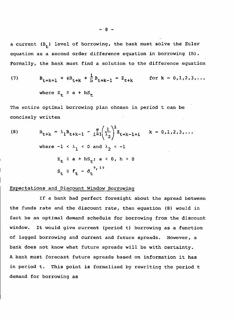
a current (Bt) level of borrowing, the bank must solve the Euler
equation as a second order difference equation in borrowing (B).
Formally, the bank must find a solution to the difference equation
(7) Bt+k+l + OBt+k + iBt+k-1 = 't+k for k = 0,1,2,3,...
where Zt % a + hSt
The entire optimal borrowing plan chosen in period t can be
concisely written
(8) i
B t+k = 'lBt+k-1 - 't+k-l+i k = 0,1,2,3,...
where -1 < Xl < 0 and A2 < -1
Zt :a+hS t; a<O,h>O
St I ft - dt 9, 10
Expectations and Discount Window Borrowing
If a bank had perfect foresight about the spread between
the funds rate and the discount rate, then equation (8) would in
fact be an optimal demand schedule for borrowing from the discount
window. It would give current (period t) borrowing as a function
of lagged borrowing and current and future spreads. However, a
bank does not know what future spreads will be with certainty.
A bank must forecast future spreads based on information it has
in period t. This point is formalized by rewriting the period t
demand for borrowing as

(9) i
Bt = Apt-1 )] - bt - hig2 x2 t-l+i'
where E[ I : the math ematical expectation conditional t
on information available in period t
In (91, the currently observable St variable has been
separated from the future spreads which must be forecast. The
E[S t-l+i] term indicates an optimal forecast of future spreads t based on information available in period t.
Equation (9) is still not a decision rule since optimal
current borrowing'Bt is not written as a function of variables that
have been observed as of period t. In order to derive a decision
rule, it is necessary to specify a process generating the spread.
For illustrative purposes, assume the spread follows a first-order
autoregressive process. In particular, suppose the S process may
be written
(10) St = aStwl + Et
where 0 c a < 1
Et 5 a random disturbance term
This process says that if S is displaced from zero, it
will return to zero asymptotically, falling back toward zero by
a proportion a each period. This means that we could forecast
future movement of S as
(11) k :[St+kl = a St

- 10 -
In other words, under the assumed simple process determining the
spread,.the only useful variable in forecasting the spread is
the current spread.
Substituting from (11) into (9) yields the following
decision rule for period t discount window borrowing
(12) Bt = yt-1 - ak + iz2(ty] - hk + iE2(+yci-l]5r
where B t L 0
-1 < Al < 0
A2 < -1
0 < a ,.< 1
O<h
O>a
Equation (12) is a decision rule or an operational demand schedule
for discount window borrowing since it shows the optimal level of
period t borrowing as a function of variables in a bank's period t
information set.
Qualitative Features of the Demand Schedule for Discount Window Borrowing
Ignore aggregation problems and consider the aggregate
demand for borrowing schedule to have the same form as (12).
The demand for borrowing has two main features. First, current
borrowing demand is negatively related to lagged borrowing.
This is a consequence of a nonprice rationing mechanism at the
discount window which discourages continuous borrowing by raising

- 11 -
the marginal perceived cost of current borrowing as borrowing
in the recent past rises. The particularly simple way in which
lagged borrowing enters is due entirely to the assumed simplicity
of the cost of borrowing function used here. In practice,
the nonprice rationing costs imposed on banks to discourage
continuous borrowing are much more complicated and difficult
to explicitly identify; so the relationship between current and
lagged borrowing is in practice difficult to specify.
Second, current borrowing demand is related to the
current spread between the funds rate and the discount rate, S t' The current spread affects current borrowings through the two
channels associated with the two terms in the coefficient on s t in
(12) l
h A higher current spread works through the "- -" term to x2
raise current borrowing demand. A higher spread works through this
channel by raising the net marginal benefit to current borrowing.
term captures the effect of the
current spread as a predictor of future spreads. Ira” plays an
important role here. A look at (11) suggests that a can be
thought of as measuring a kind of speed of adjustment or steepness
of descent of the spread toward zero after a disturbance. A
zero a means there is no inertia in the spread; it is expected
to move immediately back to zero next period. An a close to one
indicates a great deal of inertia in the spread, since it means
the spread will return to zero extremely slowly. - - The term can be written as
a (x2 - a)A2
< 0. The net coefficient on the spread may be written

- 12 -
-h >o as The derivative of the net coefficient with X2-a ' respect to a is negative. This means, for example, that a given
positive displacement of the spread from zero causes borrowing
demand to rise more the faster the expected movement of the spread
back toward zero, i.e., the smaller is a.
To see why, compare "corner"'cases where a is zero,
i.e., the displacement is purely transitory lasting just one period,
and a is near one, i.e., the displacement is more persistent. When
the high spread is purely transitory, banks expect net benefits
to borrowing and -actual borrowing to be low tomorrow. On the other
hand, if the high spread is more persistent, banks expect the net
benefits and actual borrowing to remain high tomorrow. Since the
marginal cost component of current borrowing stemming from future
planned borrowing is lower in the transitory case, the level of
current borrowing at which marginal cost just equals marginal
benefit will be reached at a higher level of current borrowing
when the spread displacement is transitory.
A particularly simple process for the spread has been
assumed to keep this example simple. If the process determining
the evolution of the spread were more complicated, the future
spread forecast embodied in the borrowing decision rule could be
a more complicated function of the current spread. It might
also involve lagged spreads and other variables if they play a
role in explaining the evolution of the spread.
It bears emphasizing that banks care about lagged
borrowing and future spreads in deciding how much to borrow

- 13 -
currently because the nonprice rationing mechanism they face at
the discount window introduces "progressive pressure" into the
cost of discount borrowing, making longer duration borrowing 11
more costly. If appropriate discount window borrowing ought to
be temporary, it is reasonable to raise the administrative
pressure on borrowing banks with the duration of their borrowing.
Duration provides an objective measure of appropriateness and
"progressive pressure" provides an automatic inducement for banks
to wean themselves from the discount window after an "emergency."
Unfortunately, although "progressive pressure" based
on duration is a useful feature of the nonprice rationing
mechanism, it introduces a dynamic element into the bank discount
window borrowing decision problem. A bank is forced to take
account of past borrowing and forecast future spreads to decide
how much to currently borrow. Not only does "progressive
pressure" make the bank's borrowing decision more difficult,
it makes the econometric task of specifying and estimating an
aggregate borrowing function for use in monetary control more
difficult as well. This last point is discussed in more
detail below.
The Borrowing Function and Fed Policy
The Federal Reserve plays a major role in the evolution
of the spread between the discount rate and the funds rate.
Movements in the spread are heavily influenced by Fed policy.
This means that rational bank forecasts of the spread must be
based on an understanding of Fed policy toward the spread. Since

- 14 -
future expected spread movements influence current borrowing
demand, not only the size of coefficients but also the form of
the borrowing function depends on Fed policy toward the spread.
The process on the spread assumed in equation (10) may
be thought of as policy induced, i.e., a policy rule. In this
view, unanticipated changes in the spread might be induced by the
Fed as part of its program for monetary control. Thereafter,
the spread's return to a normal level might be smoothed. The
size of a would be indicative of the degree of smoothing, a close
to unity indicating a greater degree of smoothing. The analysis
above has shown that the sensitivity of current borrowing to the
current spread is smaller the more smoothing or persistence
there is in deviations of the spread from a normal long run value.
The current borrowing-spread sensitivity depends on Fed policy
because the current spread appears in the borrowing function as
a predictor of future spreads.
The above analysis has implications for estimation of
the borrowing function and its use in implementing monetary policy.
First, in order to decide how much to borrow from the discount
window, banks must try to understand the Fed policy effect on the
spread. Banks must understand Fed policy toward the spread
whether it is by direct manipulation of the Federal funds and
discount rates or induced through reserve management. This means
that if the Fed wants to estimate and utilize a borrowing
function, it should make its policy intentions toward the spread
as simple and understandable as possible. Any deliberate

- 15 -
obfuscation of policy toward the spread makes it more difficult
for banks to forecast future spreads. This can only make
specification and estimation of the borrowing function
more difficult.
Second, if the Fed's implicit policy toward the spread
depends on other variables besides the spread such as recent
levels of borrowing, the money supply, or the level of interest
rates, the policy links between these other variables and the
spread should be announced explicitly. This would let banks know
what variables would help them forecast the spread and, at the
same time, let the Fed know what variables would be in the bank
borrowing function. Such a procedure would enable the Fed to
more accurately specify the borrowing function and, by implication,
to estimate and utilize it more adequately. In short, the Fed,
if it wishes to forecast bank borrowing accurately and 12
systematically, must take banks and the public into its confidence.
Third, if the Fed's implicit policy toward the spread
changes, the form of the borrowing function will change as well.
In particular, the sensitivity of current borrowing to the current
spread will depend on the implicit policy toward the spread.
This means that when the Fed makes a policy change, altering the
time series characteristics of the spread, the borrowing function
estimated over historical data from the previous policy regime
will not likely remain adequate for use in forecasting bank
borrowing under the new policy regime. If the policy change
occurs by a sequence of decisions following no clearly discussed

- 16 -
or preannounced pattern, it will become known to banks only 13
gradually. This will complicate adaptation of bank borrowing
behavior to the new policy environment and further complicate
the task of forecasting that behavior.'
Discount Window Borrowing Under Post- October 6, 1979 Reserve Targeting
The above analysis is relevant to reserve targeting as
it has been carried out by the Federal Reserve since October 6, 14
1979. The method of discount window administration in force
does not al-low the Fed to exercise direct control over total
reserves. The Fed directly controls nonborrowed reserves only.
Under this setup the Fed manipulates nonborrowed reserves to
influence the funds rate and other short-term rates of interest
and thereby affect the quantity of money demanded. The FOMC chooses
an initial intermeeting path for nonborrowed reserves designed to
induce the banking system to obtain a target volume of borrowed
reserves from the discount window. The target volume of discount
window borrowing is chosen, for a given discount rate, to produce
the desired level of the funds rate and other short-term rates of
interest and ultimately the desired effect on the money supply.
This operating procedure depends critically on the link between
discount window borrowing and the spread between the discount
rate and the funds rate, the link provided by the demand function 15
for discount window borrowing.
The Fed is having difficulty relying on the demand
function for discount window borrowing under the new operating

- 17 -
procedure. The difficulty is well described in the following
account of the means by which the FOMC chooses the initial
intermeeting target for borrowed reserves:
Typically, the Committee [FOMC] has chosen levels [an interim borrowing objective] close to the recently prevailing average --though the level chosen on October 6 was shaded higher to impose some additional initial restraint. Ideally, the assumed initial borrowing level should be such that the resultant mix of borrowed and nonborrowed reserves would tend to encourage bank behavior consistent with the emergence of desired required reserves, and hence of desired monetary growth. In practice, [for a given spread between the discount rate and the funds rate] there seem to be significant short-term variations in the willingness or desire of banks to turn to the discount window. This adds to the difficulty of choosing an appropriate level for path construction purposes, and may necessitate adjustment in a path in response to changes in bank attitudes toward the discount window.16
This account indicates that the demand for discount
window borrowing appears to the Fed as relatively volatile and 17
difficult to predict. The difficulty the Fed is having in
pinning down the borrowing function may be simply due to the
complexity and lack of uniformity of the nonprice rationing
mechanism in force at the discount window or to the irregular
use of the discount rate surcharge. However, the analysis of
this paper provides another explanation for the apparent
unreliability of the relation between borrowing demand and the
spread between the discount rate and the funds rate. First,
the analysis shows that as long as "progressive pressure" is
employed as a means of nonprice rationing, borrowing demand
depends in a potentially complicated way on lagged levels

- 18 -
of borrowing and on expected future spreads. Second, unwillingness
of the Fed to publicly specify its policy intentions toward the
spread makes it difficult for banks to form expectations about
future spreads. Both of these factors have likely contributed to
the apparent difficulty the Fed has experienced in specifying,
estimating, and utilizing a reliable borrowing function in
monetary control.
Conclusion
A demand schedule for discount window borrowing based on
profit maximizing bank behavior has been derived. The form of
the borrowing function has been shown to depend on a feature of
the nonprice rationing mechanism at the discount window that
introduces "progressive pressure" into the cost of discount window
borrowing, making longer duration borrowing more costly.
"Progressive pressure" based on duration makes lagged borrowing
and future spreads between the discount rate and the Federal funds
rate relevant to the current borrowing decision. Since movements
in the spread are heavily influenced by Fed policy, and since
expected spread movements influence borrowing demand, both the
size of the coefficients in the borr‘owing function as well as the
form of the function itself depend on Fed policy toward the spread.
This analysis is relevant to reserve targeting as it
has been carried out by the Fed since October 6, 1979. Under this
operating procedure, the demand function for discount window
borrowing has provided the critical link by which nonborrowed

- 19 -
reserve control has been made to affect short-term rates of
interest and ultimately the money supply. Unfortunately, the
relation between discount window borrowing and the spread between
the discount rate and the Federal funds rate has appeared to the
Fed as volatile and difficult to predict. This analysis suggests
that this may be the case because borrowing also depends in a
potentially complicated way ,on lagged borrowing and expected
future spreads. In addition, unwillingness -of the Fed to publicly
specify its policy intentions toward the spread makes it difficult
for banks to form expectations about future spreads. Both of
these factors have likely contributed to the difficulty the Fed
has experienced in specifying, estimating, and utilizing a
reliable borrowing function in monetary control.

FOOTNOTES
1 Federal Reserve Board Rules and Regulations,
Regulation A (as adopted effective September 1, 1980), Sec. 201.3, Par. a. Regulation A also entitles depository institutions to get seasonal and other so-called extended credit. is ignored throughout this paper.
Such borrowing
A good discussion of discount window administration is found in Board of Governors of the Federal Reserve System, "Operation of the Federal Reserve Discount Window Under the Monetary Control Act of 1980,' September 9, 1980.
2 Board of Governors of the Federal Reserve System,
Reappraisal Of the Federal Reserve Discount Mechanism, ~01s. l-3 (August 1971), p. 41;
3 See, for example, Federal Reserve Bank of San Francisco,
"Guidelines for the Administration of Short-Term Adjustment Credit in the Twelfth Federal Reserve District" (effective April 11, 1977) or Board of Governors of the Federal Reserve System, "Operation of the Federal Reserve Discount Window Under the Monetary Control Act of 1980," September 9, 1980.
4 The Depository Institutions Deregulation and Monetary
Control Act of 1980 requires all depository institutions to maintain reserves with the Federal Reserve. Included in the term depository institution are banks (whether or not they are members of the Federal Reserve System), savings banks, mutual savings banks, savings and loan associations, and credit unions. The act entitles any depository institution in which transaction accounts are held to the same discount and borrowing privileges at the Federal Reserve Banks as Federal Reserve System members. Consequently, depository institutions other than banks have access to the discount window. refer to
Since this is the case, this paper should
than 'the .depository institution borrowing decision' rather
"the bank borrowing decision." However, in the interest of simplicity the word bank is retained throughout on the understanding that'it stands for all depository institutions having access to the discount window.
5 The rate of time discount may not
be constant. But allowing for this greatly complicates the bank's maximization problem and obscures the main implications to be drawn from its solution without contributing any essential new insights.
- 20 -

- 21 -
6 A formal statement of the bank's maximization problem
is given in Appendix A. 7
this case, With no progressive pressure, cl equals zero. In the marginal cost of period t borrowing involves
Bt and dt; neither the past nor the future is relevant to the bank borrowing decision.
The linearization procedure is outlined in Appendix B. 9 The solution procedure is discussed in Sargent [1979],
Chapters 9 and 14. Without knowledge of the actual relative sizes of c
& and b, there is,no way of sufficiently restricting
the charac eristic roots of this difference equation. However, the illustrative purpose of the solution in this paper is well served by assuming that cl and b are such as to make -1 < Xl < 0 and X2 < -1. A transversality condition is obtained by assuming that if the spread between the discount rate and the funds rate were expected to be constant for all time, then planned borrowing would eventually converge to a constant optimal level.
"The optimal borrowing plan has been derived implicitly only for the case where B and f - d are both positive. Although B can never be negative and current borrowing cannot be nonzero unless current f - d is positive, these constraints have not been formally built into the solution.
11 See Footnote 7.
12 This statement is paraphrased from Lucas 119761, p. 42.
The points made in this section are based on arguments originally advanced at a more general theoretical level in Lucas' paper.
13 This statement is also paraphrased from Lucas [19761,
p. 40. 14 Technical descriptions of the post-October 6, 1979
operating procedure may be found in "Monetary Policy and Open Market Operations in 1979," pp. 60-64, "Techniques of Monetary Policy," and "The New Federal Reserve Technical Procedures for Controlling Money." Federal Reserve experience with the new operating procedure is discussed in Board of Governors of the Federal Reserve System, Federal Reserve Staff Study, New Monetary Control Procedures.
15 The Fed has allowed the funds rate to fall below the
discount rate for prolonged periods since October 6, 1979. When this happens there is no incentive for banks to borrow at the discount window, and borrowing volume becomes very small. The borrowing function plays no role in the operating procedure in such situations. Whenever the funds rate has been below the

- 22 -
discount rate, the operating strategy has essentially reverted to the pre-October 6, 1979 policy of direct funds rate control.
16 "Monetary Policy and Open Market Operations in 1979,"
Federal Reserve Bank of New York Quarterly Review (Summer 1980): 60.
17 The following comment from "Monetary Policy and
Open Market Operations in 1979," p.' 63, provides a specific illustration of the difficulty the Fed has had in utilizing the borrowing function:
The behavior of the Federal funds rate during November and December was somewhat puz.zling, as it often did not follow a usual relationship to the volume of discount window borrowings. The Federal funds rate did decline in early November, when borrowing dropped, but then continued to fall through the rest of the month, while borrowings stabilized around $1.8 bill*on to $1.9 billion. The average funds rate slipped as low as 12 l/2 percent in the final week of the month, compared with about 13 3/4 percent at the start. However, in December, when borrowings declined further, though irregularly, ranging between $1.2 billion and $1.7 billion after the first week, the funds rate jumped back up to around 13 3/4 to 14 percent through December and into January.
Normally, one would not have anticipated a drop in the Federal funds rate in late November when borrowings were steady. Nor would one have expected the rate to rise and then stay up in December as borrowings resumed their decline.
Levin and Meek [1981] and Keir [1981] contain additional evidence of the difficulty the Fed has had in using the borrowing function in monetary control.

APPENDICES
Appendix A
Maximize (at each point in time t) the discounted
present value
. y b' 't = j=O
c cO ftBt - (clBtml + 11, 4(Bt + 1)2 - 11 - dtBt 1
by choosing a sequence for {B t+j'jlo subject to Btml = ztml, a
transversality condition and a known sequence {f t+j - dt+j j=O* lW
Appendix B
A linear approximation to the Euler equation is
constructed as follows. Define AXt a Xt - X L , where X L is a long
run value. Then
[cl(BL + ABtWl) + llcO(BL + ABt + 1)
+bCTo -[(BL + ABt+l + 1)2 - 11 = (f - d)L + A(ft - dt)
Assume B L is small and redefine Bt Z AB t' so that the
linearized Euler equation may be written
B 1 t+1 +qBt+ ;BtWl = -
+ BL(cocl + co + bclcO)
bCICO I
+ bc;co(ft - dt)
- 23 -

REFERENCES
Board of Governors of the Federal Reserve System. Federal Reserve Board Rules and Regulations, Regulation A (as adopted effective September 1, 1980).
"Operation of the Federal Reserve Discount Window Under the Monetary Control Act of 1980," September 9, 1980.
Reappraisal of the Federal Reserve Discount Mechanism (&s. l-3) : August 1971.
Depository Institutions Deregulation and Monetary Control Act of 1980, PL 96-221, March 31, 1980.
Federal Reserve Bank of San Francisco. "Guidelines for the Administration of Short-Term Adjustment Credit in the Twelfth Federal Reserve District," effective April 11, 1977.
Keir, Peter. "Impact of Discount Policy Procedures on the Effectiveness of Reserve Targeting." In Federal Reserve Staff Study--Volume l,.New Monetary Control Procedures. Board of Governors of the Federal Reserve System, February 1981.
Levin, Fred, and Meek, Paul. "Implementing the New Operating Procedures: The View from the Trading Desk." In Federal Reserve Staff Study--Volume 1, New Monetary Control Procedures. Board of Governors of the Federal Reserve System, February 1981.
Lucas, Robert E., Jr. "Econometric Policy Evaluation: A Critique." In The Phillips Curve and Labor Markets, ed. K. Brunner and A. H. Meltzer. Carnegie-Rochester Conference Series on Public Policy 1: 19-46. Amsterdam: North Holland, 1976.
"Monetary Policy and Open Market Operations in 1979." Federal Reserve Bank of New York Quarterly Review (Summer 1980): 50-64.
"The New Federal Reserve Technical Procedures for Controlling Money." Appendix to a statement by Paul A. Volcker, Chairman, Board of Governors of the Federal Reserve System before the Joint Economic Committee, February 1, 1980. Subsequently published in U.S., Congress, House, Committee
- 24 -

- 25 -
on Banking, Finance, and Urban Affairs, Conduct of Monetary Policy (Pursuant to the Full Employment and Balanced Growth Act of 1978, P.L. 95-523), Hearing, February 19, 1980 (Washington, D.C.: U.S. Government Printing Office, 1980), pp. 108-15.
Sargent, Thomas. Macroeconomic Theory. New York: Academic Press, 1979.
"Techniques of Monetary Policy." Remarks by Henry C. Wallich, Member, Board of Governors of the Federal Reserve System at a meeting of the Missouri Valley Economic Association, Memphis, Tenn., on March 1, 1980.
Recommended