1
Direct and indirect effects based on difference-in-differences
with an application to political preferences following the Vietnam draft lottery
Eva Deuchert, Martin Huber, Mark Schelker
University of Fribourg, Department of Economics
Abstract: This paper proposes a difference-in-differences approach for disentangling a total
treatment effect on some outcome into a direct impact as well as an indirect effect operating
through a binary intermediate variable – or mediator – within strata defined upon how the mediator
reacts to the treatment. We show under which assumptions the direct effects on the always and
never takers, whose mediator is not affected by the treatment, as well as the direct and indirect
effects on the compliers, whose mediator reacts to the treatment, are identified. We provide an
empirical application based on the Vietnam draft lottery. The results suggest that a high draft risk
due to the lottery leads to a relative increase in the support for the Republican Party and that this
increase is mostly driven by those complying with the lottery outcome.
Keywords: treatment effects, causal mechanisms, direct and indirect effects, Vietnam War
lottery, political preferences
JEL classification: C21, C22, D70, D72
We have benefitted from comments by seminar participants in Hong Kong (HKUST) and Taipei (Academia Sinica).
Addresses for correspondence: Eva Deuchert ([email protected]), Martin Huber ([email protected]),
Mark Schelker ([email protected]), University of Fribourg, Department of Economics, Bd. de Pérolles 90, 1700
Fribourg, Switzerland.
2
1 Introduction
Policy and treatment evaluation typically aims at assessing the causal effect of an intervention or
treatment on an outcome of interest. In many cases, however, not only the (total) treatment effect
appears interesting, but also the causal mechanisms through which it materializes. Causal
mediation analysis (Robins and Greenland, 1992; Pearl, 2001; Robins, 2003) therefore aims at
disentangling the direct effect of the treatment on the outcome as well as the indirect effects
operating through one or more intermediate variables, also called mediators.
The main contribution of this paper is the proposition of a difference-in-differences (DiD)
approach for separating direct and indirect effects within subpopulations (or strata) defined upon
the reaction of a binary mediator to the treatment. Borrowing from the nomenclature in Angrist,
Imbens, and Rubin (1996), we demonstrate under which assumptions direct effects for “always”
and “never takers”, whose binary mediator is independent of the treatment always or never one, or
of the direct and indirect effects on the compliers, whose mediator value always corresponds to the
treatment state, are identified. Among others, random treatment assignment, monotonicity of the
mediator in the treatment, and specific common trend assumptions across strata are imposed for
identification.
In contrast to our approach, a good part of the literature on causal mediation analysis assumes
conditional exogeneity of the treatment (given observed covariates) and the mediator (given the
treatment and the covariates), which requires observing all confounders of the treatment and the
mediator. Such “sequential ignorability” is for instance imposed in Petersen, Sinisi, and van der
Laan (2006), Flores and Flores-Lagunes (2009), VanderWeele (2009), Imai, Keele, and Yamamoto
(2010), Hong (2010), Tchetgen Tchetgen and Shpitser (2012), Zheng and van der Laan (2012), and
Huber (2014). Alternatively, relatively few contributions consider identification based on
instruments, see for instance Imai, Tingley, and Yamamoto (2013), Yamamoto (2013), and Frölich
3
and Huber (2014). Our paper is to the best of our knowledge the first one to offer an alternative to
sequential ignorability and instrumental variable assumptions based on a DiD approach in the
context of mediation analysis.
While most mediation studies focus on the total population, comparably few contributions
discuss effects in subpopulations (or principal strata, see Frangakis and Rubin, 2002) defined upon
the value of the binary mediator as a function of the treatment, see for instance Rubin (2004).
Principal stratification in the context of mediation has been criticized for typically not permitting a
decomposition of direct and indirect effects among compliers and focussing on subgroups that may
be less interesting than the entire population, see VanderWeele (2008; 2012). We contribute to this
discussion by showing that direct and indirect effects on compliers are identified in a DiD
framework under particular conditions and by presenting an empirical application in which the
effect on subgroups is relevant for political decision making.
We apply our method to investigate the effect of the Vietnam draft lottery in the years 1969 to
1972 in the US on political preferences, personal views on war policies, and personal attitudes. Our
mediator of interest is military service during the Vietnam War. We note that a subset of
individuals (compliers) was induced by the lottery to serve in the army either through being drafted
or “voluntarily” joining the military in case of an unfavourable lottery outcome (Angrist, 1991),
while others avoided the draft (never takers) for instance through college deferments (Card and
Lemieux, 2001; Kuziemko, 2010; Deuchert and Huber, 2014), or would have served in any case
(always takers). We aim at estimating the direct effects of the draft lottery on the never takers, as
well as the direct and indirect effect (via military service) on the compliers.
This is a particularly interesting application for several reasons: First, the recent literature
argues that party preferences and political attitudes are endogenous to policy changes (Bergan,
4
2009; Erikson and Stoker, 2011), which is in contrast to most economic models. Erikson and
Stoker (2011) use the Vietnam draft lottery to estimate the impact of receiving an unfavourable
lottery number on party preferences and political attitudes in a highly selected sample of young
college-bound men and conclude that a change in the draft risk increases support for the
Democratic Party. Using a sample of 115 male students from the 1972 class of the University of
Virginia, Bergan (2009) shows that the draft induced those with unfavourable lottery numbers to be
more strongly in favour of an immediate withdrawal from Vietnam. We challenge these results,
estimating the impact of the draft on political preferences in a more representative sample. Second,
we go beyond the intention to treat effect and specifically consider heterogeneity in the response to
the draft across strata. The previous literature analysing the impact of the Vietnam War lottery
typically assumes that the Vietnam War lottery impacts outcomes only via military service and thus
assumes that the direct effect of the lottery is equal to zero (Angrist, Chen, and Frandsen, 2010;
Angrist, 1990) for any population. We challenge this assumption, too.
In contrast to Erikson and Stoker (2011) and Bergan (2009), we find that the draft lottery
significantly increases the probability to vote Republican, but has no effects on Vietnam War
attitudes. When decomposing the average treatment effect into direct and indirect effects within
strata, the electoral results are no longer significant. Taken at face value, the point estimates
suggest that the overall effect appears to be largely driven by compliers who increase their relative
support for the Republicans. However, both the total and indirect effects on compliers are far
smaller than the local average treatment effect (LATE) estimate on compliers, which relies on the
lottery being a valid instrument for military service. This points to the non-robustness of the results
across various econometric approaches, as the true LATE equals the true indirect effect among
compliers (for whom the first stage is one by definition) in the absence of direct effects.
5
The remainder of this paper is organized as follows. Section 2 outlines the econometric
framework, i.e., the effects of interest and the identifying assumptions underlying our DiD
approach. Section 3 presents an empirical application to the Vietnam draft lottery in which the total
effects as well as the direct and indirect effects on political preferences and personal views on war
and other governmental policies are estimated for various strata. Section 4 concludes. The
appendix includes among other a simulation study to provide some intuition for scenarios in which
the various identifying assumptions are satisfied or violated.
2 Econometric framework
2.1 Notation and definition of direct and indirect effects
Let 𝑍 denote a binary treatment (e.g., being chosen for military service in a draft lottery) and 𝐷 a
binary intermediate variable or mediator that may be a function of 𝑍 (e.g., an indicator for actual
military service). Furthermore, let 𝑇 indicate a particular time period: 𝑇 = 0 denotes the baseline
period prior to assignment of 𝑍 and 𝐷, 𝑇 = 1 the follow up period after measuring 𝐷 and 𝑍 in
which the effect of the outcome is evaluated. Finally, let 𝑌𝑡 denote the outcome of interest (e.g.,
political preference) in period 𝑇 = 𝑡. Indexing the outcome by the time period 𝑡 ∈ {1,0} implies
that it may be measured both in the baseline period and after the assignment of 𝑍 and 𝐷. To define
the parameters of interest, we make use of the potential outcome notation, see for instance Rubin
(1974), and denote by 𝑌𝑡(𝑧, 𝑑) the potential outcome for treatment state 𝑍 = 𝑧 and mediator state
𝐷 = 𝑑 in time 𝑇 = 𝑡, with 𝑧, 𝑑, 𝑡 ∈ {1,0}. Furthermore, let 𝐷(𝑧) denote the potential mediator as
a function of the treatment state 𝑧 ∈ {1,0}. For notational ease, we will not use a time index for 𝐷
and 𝑍, because each of these parameters are assumed to be measured at a single period between
𝑇 = 0 and 𝑇 = 1 (but not necessarily the same period, as 𝐷 causally precedes 𝑍).
6
Using this notation, the average treatment effect (ATE) in the follow up period is defined as
∆1= 𝐸[𝑌1(1, 𝐷(1)) − 𝑌1(0, 𝐷(0))]. That is, the ATE corresponds to the cumulative effect of 𝑍 on
the outcome that either affects the latter directly (i.e., net of any effect on the mediator) or
indirectly through an effect on 𝐷. Indeed, the total ATE can be disentangled into the direct and
indirect effects, denoted by 𝜃1(𝑧) = 𝐸[𝑌1(1, 𝐷(𝑧)) − 𝑌1(0, 𝐷(𝑧))] and
𝛿1(𝑧) = 𝐸[𝑌1(𝑧, 𝐷(1)) − 𝑌1(𝑧, 𝐷(0))], by adding and subtracting 𝑌1(1, 𝐷(0)) or 𝑌1(0, 𝐷(1)),
respectively:
∆1= 𝐸[𝑌1(1, 𝐷(1)) − 𝑌1(0, 𝐷(0))]
= 𝐸[𝑌1(1, 𝐷(0)) − 𝑌1(0, 𝐷(0))] + 𝐸[𝑌1(1, 𝐷(1)) − 𝑌1(1, 𝐷(0))]
= 𝜃1(0) + 𝛿1(1)
= 𝐸[𝑌1(1, 𝐷(1)) − 𝑌1(0, 𝐷(1))] + 𝐸[𝑌1(0, 𝐷(1)) − 𝑌1(0, 𝐷(0))]
= 𝜃1(1) + 𝛿1(0)
Distinguishing between 𝜃1(1) and 𝜃1(0) or 𝛿1(1) and 𝛿1(0) , respectively, implies the
possibility of interaction effects between 𝑍 and 𝐷 such that the effects could be heterogeneous
across values 𝑧 = 1 and 𝑧 = 0. For instance, 𝛿1(1) and 𝛿1(1) might differ if the military unit
(and war experience) one is assigned to when being chosen through the draft lottery is different
than when joining the army voluntarily without being drafted, which may have an impact on
political attitude. Furthermore, note that if 𝑍 was a valid instrument for 𝐷 that satisfied the
exclusion restriction, as for instance assumed in Angrist (1990) in the context of the Vietnam draft
lottery, any direct effect 𝜃𝑡(𝑧) would be zero and the indirect 𝛿1(1) = 𝛿1(0) = 𝛿1 would
correspond to the so-called intention to treat effect. In our empirical application outlined below, we
do not impose this strong assumption, which has for instance been challenged in Deuchert and
Huber (2014), but explicitly allow for direct effects.
7
In our approach we consider the concepts of direct and indirect effects within subgroups or
so-called principal strata in the denomination of Frangakis and Rubin (2002) that are defined upon
the values of the potential mediator. As outlined in Angrist, Imbens, and Rubin (1996) in the
context of instrumental variable-based identification, any individual 𝑖 in the population belongs to
one of four strata, henceforth denoted by 𝜏, according to their potential mediator status (now
indexed by 𝑖) under either treatment state: always takers (𝑎: 𝐷𝑖(1) = 𝐷𝑖(0) = 1) whose mediator
is always one, compliers (𝑐: 𝐷𝑖(1) = 1, 𝐷𝑖(0) = 0) whose mediator corresponds to the treatment
value, defiers (𝑑: 𝐷𝑖(1) = 0, 𝐷𝑖(0) = 1) whose mediator opposes the treatment value, and never
takers (𝑛: 𝐷𝑖(1) = 𝐷𝑖(0) = 0) whose mediator is never one. Note that 𝜏 cannot be pinned down
for any individual, because either 𝐷𝑖(1) or 𝐷𝑖(0) is observed, but never both.
Introducing some further stratum-specific notation, let ∆1𝜏= 𝐸[𝑌1(1, 𝐷(1)) − 𝑌1(0, 𝐷(0))|𝜏]
denote the ATE conditional on 𝜏 ∈ {𝑎, 𝑛, 𝑐, 𝑑}; 𝜃1𝜏(𝑧) and 𝛿1
𝜏(𝑧) denote the corresponding direct
and indirect effects. Because 𝐷𝑖(1) = 𝐷𝑖(0) = 0 for any never taker, the indirect effect for this
group is by definition zero (𝛿1𝑛(𝑧) = 𝐸[𝑌1(𝑧, 0) − 𝑌1(𝑧, 0)|𝑛] = 0) and ∆1
𝑛= 𝐸[𝑌1(1,0) −
𝑌1(0,0)|𝑛] = 𝜃1𝑛(1) = 𝜃1
𝑛(0) = 𝜃1𝑛 corresponds to the direct effect (and an analogous argument
applies to the always takers). For the compliers, both direct and indirect effects may exist. Note that
𝐷(𝑧) = 𝑧 due to the definition of compliers. Therefore, 𝜃1𝑐(𝑧) = 𝐸[𝑌1(1, 𝑧) − 𝑌1(0, 𝑧)|𝑐] and
𝛿1𝑐(𝑧) = 𝐸[𝑌1(𝑧, 1) − 𝑌1(𝑧, 0)|𝑐]. Furthermore, in the absence of any direct effect, the indirect
effects on the compliers are homogenous, 𝛿1𝑐(1) = 𝛿1
𝑐(0) = 𝛿1𝑐, and correspond to the LATE.
2.2 Identifying assumptions
We subsequently discuss the identifying assumptions along with the effects that may be obtained.
We start by assuming independence between the treatment and potential mediators or outcomes:
8
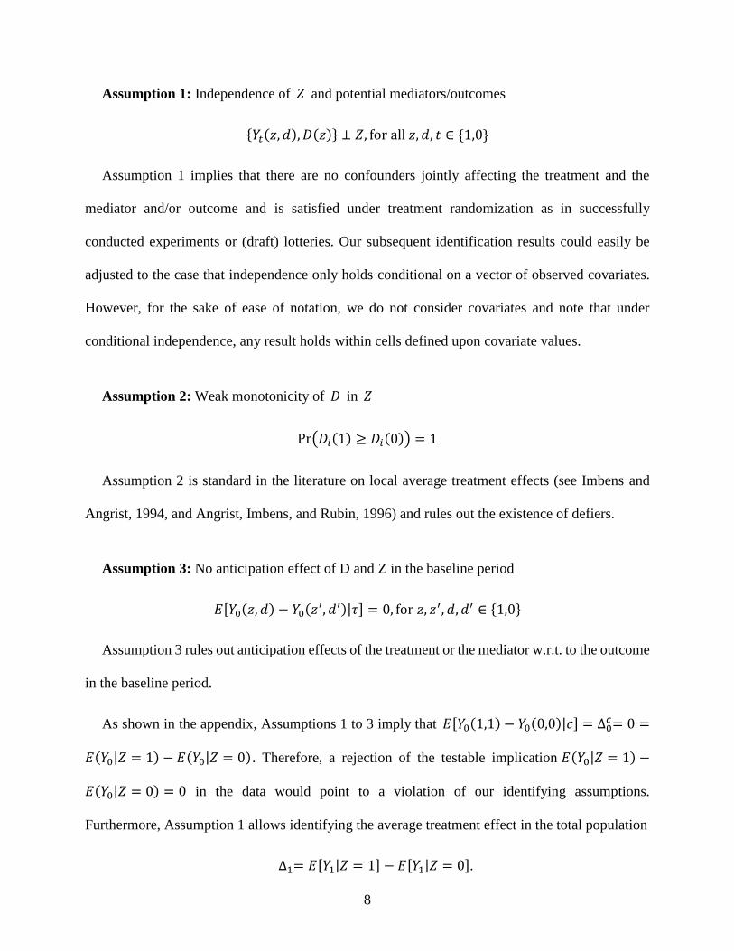
Assumption 1: Independence of 𝑍 and potential mediators/outcomes
{𝑌𝑡(𝑧, 𝑑), 𝐷(𝑧)} ⊥ 𝑍, for all 𝑧, 𝑑, 𝑡 ∈ {1,0}
Assumption 1 implies that there are no confounders jointly affecting the treatment and the
mediator and/or outcome and is satisfied under treatment randomization as in successfully
conducted experiments or (draft) lotteries. Our subsequent identification results could easily be
adjusted to the case that independence only holds conditional on a vector of observed covariates.
However, for the sake of ease of notation, we do not consider covariates and note that under
conditional independence, any result holds within cells defined upon covariate values.
Assumption 2: Weak monotonicity of 𝐷 in 𝑍
Pr(𝐷𝑖(1) ≥ 𝐷𝑖(0)) = 1
Assumption 2 is standard in the literature on local average treatment effects (see Imbens and
Angrist, 1994, and Angrist, Imbens, and Rubin, 1996) and rules out the existence of defiers.
Assumption 3: No anticipation effect of D and Z in the baseline period
𝐸[𝑌0(𝑧, 𝑑) − 𝑌0(𝑧′, 𝑑′)|𝜏] = 0, for 𝑧, 𝑧′, 𝑑, 𝑑′ ∈ {1,0}
Assumption 3 rules out anticipation effects of the treatment or the mediator w.r.t. to the outcome
in the baseline period.
As shown in the appendix, Assumptions 1 to 3 imply that 𝐸[𝑌0(1,1) − 𝑌0(0,0)|𝑐] = ∆0𝑐= 0 =
𝐸(𝑌0|𝑍 = 1) − 𝐸(𝑌0|𝑍 = 0). Therefore, a rejection of the testable implication 𝐸(𝑌0|𝑍 = 1) −
𝐸(𝑌0|𝑍 = 0) = 0 in the data would point to a violation of our identifying assumptions.
Furthermore, Assumption 1 allows identifying the average treatment effect in the total population
∆1= 𝐸[𝑌1|𝑍 = 1] − 𝐸[𝑌1|𝑍 = 0].
9
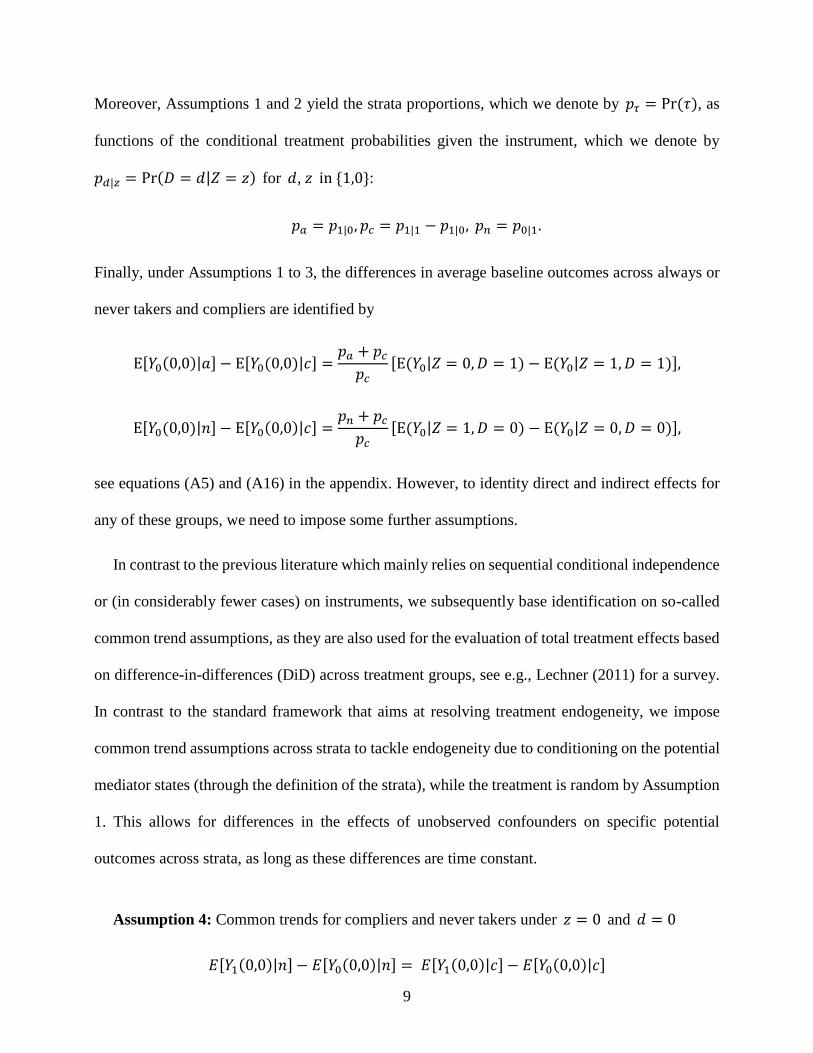
Moreover, Assumptions 1 and 2 yield the strata proportions, which we denote by 𝑝𝜏 = Pr (𝜏), as
functions of the conditional treatment probabilities given the instrument, which we denote by
𝑝𝑑|𝑧 = Pr(𝐷 = 𝑑|𝑍 = 𝑧) for 𝑑, 𝑧 in {1,0}:
𝑝𝑎 = 𝑝1|0, 𝑝𝑐 = 𝑝1|1 − 𝑝1|0, 𝑝𝑛 = 𝑝0|1.
Finally, under Assumptions 1 to 3, the differences in average baseline outcomes across always or
never takers and compliers are identified by
E[𝑌0(0,0)|𝑎] − E[𝑌0(0,0)|𝑐] =𝑝𝑎 + 𝑝𝑐
𝑝𝑐
[E(𝑌0|𝑍 = 0, 𝐷 = 1) − E(𝑌0|𝑍 = 1, 𝐷 = 1)],
E[𝑌0(0,0)|𝑛] − E[𝑌0(0,0)|𝑐] =𝑝𝑛 + 𝑝𝑐
𝑝𝑐
[E(𝑌0|𝑍 = 1, 𝐷 = 0) − E(𝑌0|𝑍 = 0, 𝐷 = 0)],
see equations (A5) and (A16) in the appendix. However, to identity direct and indirect effects for
any of these groups, we need to impose some further assumptions.
In contrast to the previous literature which mainly relies on sequential conditional independence
or (in considerably fewer cases) on instruments, we subsequently base identification on so-called
common trend assumptions, as they are also used for the evaluation of total treatment effects based
on difference-in-differences (DiD) across treatment groups, see e.g., Lechner (2011) for a survey.
In contrast to the standard framework that aims at resolving treatment endogeneity, we impose
common trend assumptions across strata to tackle endogeneity due to conditioning on the potential
mediator states (through the definition of the strata), while the treatment is random by Assumption
1. This allows for differences in the effects of unobserved confounders on specific potential
outcomes across strata, as long as these differences are time constant.
Assumption 4: Common trends for compliers and never takers under 𝑧 = 0 and 𝑑 = 0
𝐸[𝑌1(0,0)|𝑛] − 𝐸[𝑌0(0,0)|𝑛] = 𝐸[𝑌1(0,0)|𝑐] − 𝐸[𝑌0(0,0)|𝑐]
10
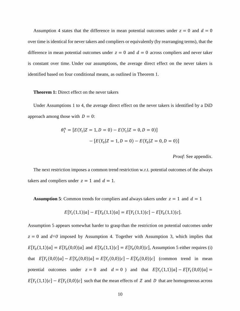
Assumption 4 states that the difference in mean potential outcomes under 𝑧 = 0 and 𝑑 = 0
over time is identical for never takers and compliers or equivalently (by rearranging terms), that the
difference in mean potential outcomes under 𝑧 = 0 and 𝑑 = 0 across compliers and never taker
is constant over time. Under our assumptions, the average direct effect on the never takers is
identified based on four conditional means, as outlined in Theorem 1.
Theorem 1: Direct effect on the never takers
Under Assumptions 1 to 4, the average direct effect on the never takers is identified by a DiD
approach among those with 𝐷 = 0:
𝜃1𝑛 = [𝐸(𝑌1|𝑍 = 1, 𝐷 = 0) − 𝐸(𝑌1|𝑍 = 0, 𝐷 = 0)]
− [𝐸(𝑌0|𝑍 = 1, 𝐷 = 0) − 𝐸(𝑌0|𝑍 = 0, 𝐷 = 0)]
Proof: See appendix.
The next restriction imposes a common trend restriction w.r.t. potential outcomes of the always
takers and compliers under 𝑧 = 1 and 𝑑 = 1.
Assumption 5: Common trends for compliers and always takers under 𝑧 = 1 and 𝑑 = 1
𝐸[𝑌1(1,1)|𝑎] − 𝐸[𝑌0(1,1)|𝑎] = 𝐸[𝑌1(1,1)|𝑐] − 𝐸[𝑌0(1,1)|𝑐].
Assumption 5 appears somewhat harder to grasp than the restriction on potential outcomes under
𝑧 = 0 and d=0 imposed by Assumption 4. Together with Assumption 3, which implies that
𝐸[𝑌0(1,1)|𝑎] = 𝐸[𝑌0(0,0)|𝑎] and 𝐸[𝑌0(1,1)|𝑐] = 𝐸[𝑌0(0,0)|𝑐], Assumption 5 either requires (i)
that 𝐸[𝑌1(0,0)|𝑎] − 𝐸[𝑌0(0,0)|𝑎] = 𝐸[𝑌1(0,0)|𝑐] − 𝐸[𝑌0(0,0)|𝑐] (common trend in mean
potential outcomes under 𝑧 = 0 and 𝑑 = 0 ) and that 𝐸[𝑌1(1,1)|𝑎] − 𝐸[𝑌1(0,0)|𝑎] =
𝐸[𝑌1(1,1)|𝑐] − 𝐸[𝑌1(0,0)|𝑐] such that the mean effects of 𝑍 and 𝐷 that are homogeneous across
11
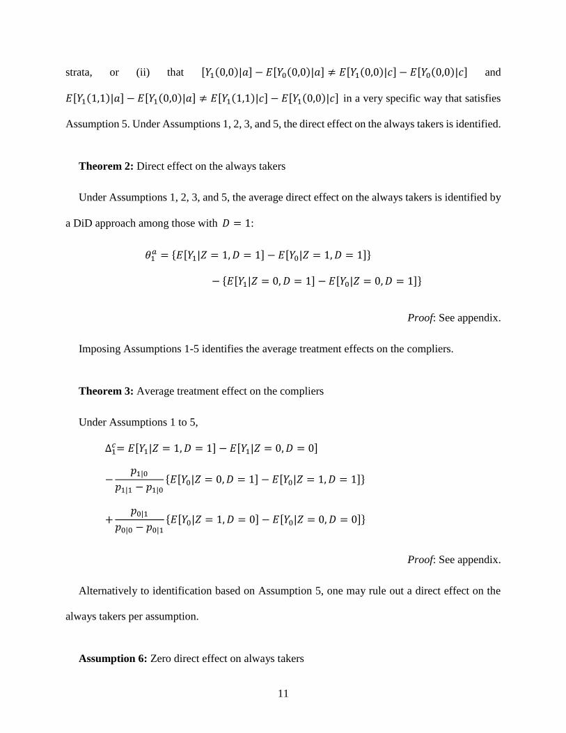
strata, or (ii) that [𝑌1(0,0)|𝑎] − 𝐸[𝑌0(0,0)|𝑎] ≠ 𝐸[𝑌1(0,0)|𝑐] − 𝐸[𝑌0(0,0)|𝑐] and
𝐸[𝑌1(1,1)|𝑎] − 𝐸[𝑌1(0,0)|𝑎] ≠ 𝐸[𝑌1(1,1)|𝑐] − 𝐸[𝑌1(0,0)|𝑐] in a very specific way that satisfies
Assumption 5. Under Assumptions 1, 2, 3, and 5, the direct effect on the always takers is identified.
Theorem 2: Direct effect on the always takers
Under Assumptions 1, 2, 3, and 5, the average direct effect on the always takers is identified by
a DiD approach among those with 𝐷 = 1:
𝜃1𝑎 = {𝐸[𝑌1|𝑍 = 1, 𝐷 = 1] − 𝐸[𝑌0|𝑍 = 1, 𝐷 = 1]}
− {𝐸[𝑌1|𝑍 = 0, 𝐷 = 1] − 𝐸[𝑌0|𝑍 = 0, 𝐷 = 1]}
Proof: See appendix.
Imposing Assumptions 1-5 identifies the average treatment effects on the compliers.
Theorem 3: Average treatment effect on the compliers
Under Assumptions 1 to 5,
∆1𝑐= 𝐸[𝑌1|𝑍 = 1, 𝐷 = 1] − 𝐸[𝑌1|𝑍 = 0, 𝐷 = 0]
−𝑝1|0
𝑝1|1 − 𝑝1|0
{𝐸[𝑌0|𝑍 = 0, 𝐷 = 1] − 𝐸[𝑌0|𝑍 = 1, 𝐷 = 1]}
+𝑝0|1
𝑝0|0 − 𝑝0|1
{𝐸[𝑌0|𝑍 = 1, 𝐷 = 0] − 𝐸[𝑌0|𝑍 = 0, 𝐷 = 0]}
Proof: See appendix.
Alternatively to identification based on Assumption 5, one may rule out a direct effect on the
always takers per assumption.
Assumption 6: Zero direct effect on always takers
12
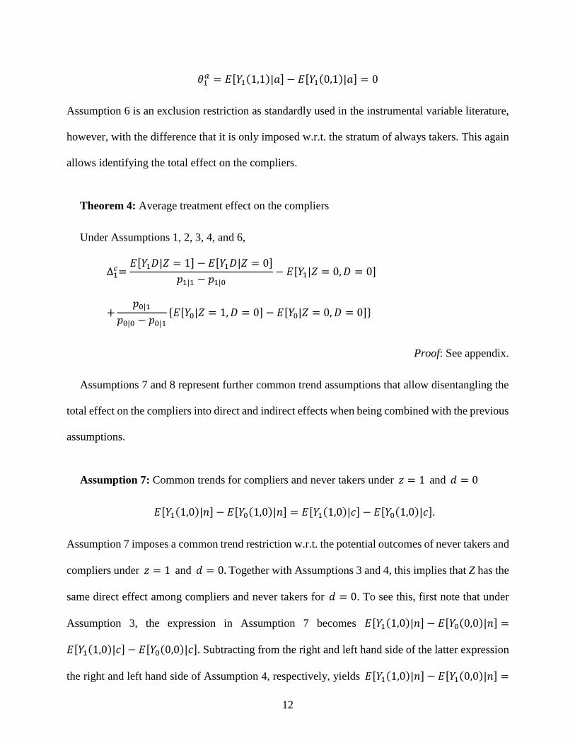
𝜃1𝑎 = 𝐸[𝑌1(1,1)|𝑎] − 𝐸[𝑌1(0,1)|𝑎] = 0
Assumption 6 is an exclusion restriction as standardly used in the instrumental variable literature,
however, with the difference that it is only imposed w.r.t. the stratum of always takers. This again
allows identifying the total effect on the compliers.
Theorem 4: Average treatment effect on the compliers
Under Assumptions 1, 2, 3, 4, and 6,
∆1𝑐=
𝐸[𝑌1𝐷|𝑍 = 1] − 𝐸[𝑌1𝐷|𝑍 = 0]
𝑝1|1 − 𝑝1|0− 𝐸[𝑌1|𝑍 = 0, 𝐷 = 0]
+𝑝0|1
𝑝0|0 − 𝑝0|1
{𝐸[𝑌0|𝑍 = 1, 𝐷 = 0] − 𝐸[𝑌0|𝑍 = 0, 𝐷 = 0]}
Proof: See appendix.
Assumptions 7 and 8 represent further common trend assumptions that allow disentangling the
total effect on the compliers into direct and indirect effects when being combined with the previous
assumptions.
Assumption 7: Common trends for compliers and never takers under 𝑧 = 1 and 𝑑 = 0
𝐸[𝑌1(1,0)|𝑛] − 𝐸[𝑌0(1,0)|𝑛] = 𝐸[𝑌1(1,0)|𝑐] − 𝐸[𝑌0(1,0)|𝑐].
Assumption 7 imposes a common trend restriction w.r.t. the potential outcomes of never takers and
compliers under 𝑧 = 1 and 𝑑 = 0. Together with Assumptions 3 and 4, this implies that Z has the
same direct effect among compliers and never takers for 𝑑 = 0. To see this, first note that under
Assumption 3, the expression in Assumption 7 becomes 𝐸[𝑌1(1,0)|𝑛] − 𝐸[𝑌0(0,0)|𝑛] =
𝐸[𝑌1(1,0)|𝑐] − 𝐸[𝑌0(0,0)|𝑐]. Subtracting from the right and left hand side of the latter expression
the right and left hand side of Assumption 4, respectively, yields 𝐸[𝑌1(1,0)|𝑛] − 𝐸[𝑌1(0,0)|𝑛] =
13
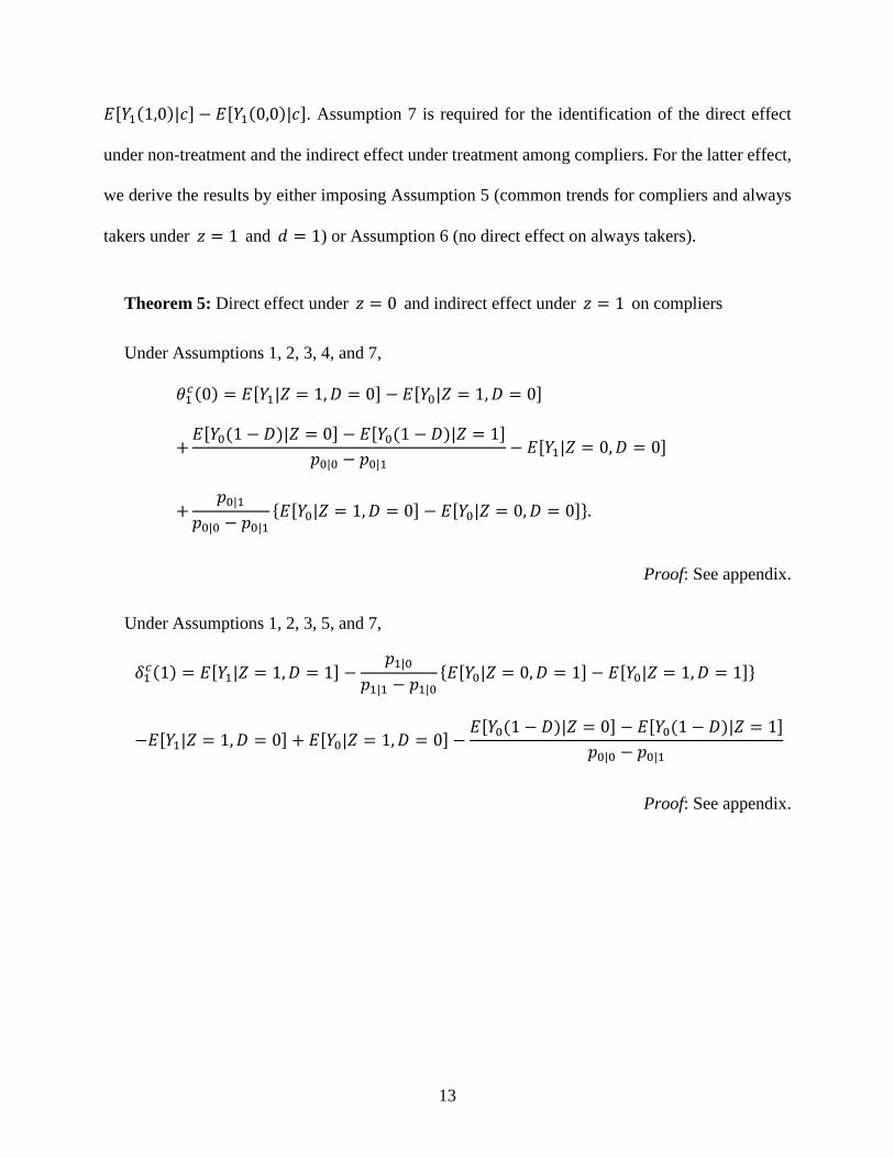
𝐸[𝑌1(1,0)|𝑐] − 𝐸[𝑌1(0,0)|𝑐]. Assumption 7 is required for the identification of the direct effect
under non-treatment and the indirect effect under treatment among compliers. For the latter effect,
we derive the results by either imposing Assumption 5 (common trends for compliers and always
takers under 𝑧 = 1 and 𝑑 = 1) or Assumption 6 (no direct effect on always takers).
Theorem 5: Direct effect under 𝑧 = 0 and indirect effect under 𝑧 = 1 on compliers
Under Assumptions 1, 2, 3, 4, and 7,
𝜃1𝑐(0) = 𝐸[𝑌1|𝑍 = 1, 𝐷 = 0] − 𝐸[𝑌0|𝑍 = 1, 𝐷 = 0]
+𝐸[𝑌0(1 − 𝐷)|𝑍 = 0] − 𝐸[𝑌0(1 − 𝐷)|𝑍 = 1]
𝑝0|0 − 𝑝0|1− 𝐸[𝑌1|𝑍 = 0, 𝐷 = 0]
+𝑝0|1
𝑝0|0 − 𝑝0|1
{𝐸[𝑌0|𝑍 = 1, 𝐷 = 0] − 𝐸[𝑌0|𝑍 = 0, 𝐷 = 0]}.
Proof: See appendix.
Under Assumptions 1, 2, 3, 5, and 7,
𝛿1𝑐(1) = 𝐸[𝑌1|𝑍 = 1, 𝐷 = 1] −
𝑝1|0
𝑝1|1 − 𝑝1|0
{𝐸[𝑌0|𝑍 = 0, 𝐷 = 1] − 𝐸[𝑌0|𝑍 = 1, 𝐷 = 1]}
−𝐸[𝑌1|𝑍 = 1, 𝐷 = 0] + 𝐸[𝑌0|𝑍 = 1, 𝐷 = 0] −𝐸[𝑌0(1 − 𝐷)|𝑍 = 0] − 𝐸[𝑌0(1 − 𝐷)|𝑍 = 1]
𝑝0|0 − 𝑝0|1
Proof: See appendix.
14
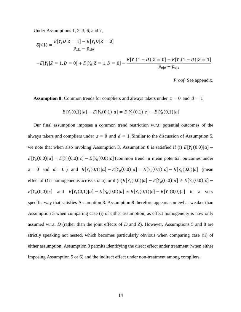
Under Assumptions 1, 2, 3, 6, and 7,
𝛿1𝑐(1) =
𝐸[𝑌1𝐷|𝑍 = 1] − 𝐸[𝑌1𝐷|𝑍 = 0]
𝑝1|1 − 𝑝1|0
−𝐸[𝑌1|𝑍 = 1, 𝐷 = 0] + 𝐸[𝑌0|𝑍 = 1, 𝐷 = 0] −𝐸[𝑌0(1 − 𝐷)|𝑍 = 0] − 𝐸[𝑌0(1 − 𝐷)|𝑍 = 1]
𝑝0|0 − 𝑝0|1
Proof: See appendix.
Assumption 8: Common trends for compliers and always takers under 𝑧 = 0 and 𝑑 = 1
𝐸[𝑌1(0,1)|𝑎] − 𝐸[𝑌0(0,1)|𝑎] = 𝐸[𝑌1(0,1)|𝑐] − 𝐸[𝑌0(0,1)|𝑐]
Our final assumption imposes a common trend restriction w.r.t. potential outcomes of the
always takers and compliers under 𝑧 = 0 and 𝑑 = 1. Similar to the discussion of Assumption 5,
we note that when also invoking Assumption 3, Assumption 8 is satisfied if (i) 𝐸[𝑌1(0,0)|𝑎] −
𝐸[𝑌0(0,0)|𝑎] = 𝐸[𝑌1(0,0)|𝑐] − 𝐸[𝑌0(0,0)|𝑐] (common trend in mean potential outcomes under
𝑧 = 0 and 𝑑 = 0 ) and 𝐸[𝑌1(0,1)|𝑎] − 𝐸[𝑌0(0,0)|𝑎] = 𝐸[𝑌1(0,1)|𝑐] − 𝐸[𝑌0(0,0)|𝑐] (mean
effect of D is homogeneous across strata), or if (ii)𝐸[𝑌1(0,0)|𝑎] − 𝐸[𝑌0(0,0)|𝑎] ≠ 𝐸[𝑌1(0,0)|𝑐] −
𝐸[𝑌0(0,0)|𝑐] and 𝐸[𝑌1(0,1)|𝑎] − 𝐸[𝑌0(0,0)|𝑎] ≠ 𝐸[𝑌1(0,1)|𝑐] − 𝐸[𝑌0(0,0)|𝑐] in a very
specific way that satisfies Assumption 8. Assumption 8 therefore appears somewhat weaker than
Assumption 5 when comparing case (i) of either assumption, as effect homogeneity is now only
assumed w.r.t. D (rather than the joint effects of D and Z). However, Assumptions 5 and 8 are
strictly speaking not nested, which becomes particularly obvious when comparing case (ii) of
either assumption. Assumption 8 permits identifying the direct effect under treatment (when either
imposing Assumption 5 or 6) and the indirect effect under non-treatment among compliers.
15
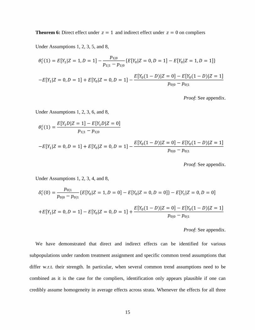
Theorem 6: Direct effect under 𝑧 = 1 and indirect effect under 𝑧 = 0 on compliers
Under Assumptions 1, 2, 3, 5, and 8,
𝜃1𝑐(1) = 𝐸[𝑌1|𝑍 = 1, 𝐷 = 1] −
𝑝1|0
𝑝1|1 − 𝑝1|0
{𝐸[𝑌0|𝑍 = 0, 𝐷 = 1] − 𝐸[𝑌0|𝑍 = 1, 𝐷 = 1]}
−𝐸[𝑌1|𝑍 = 0, 𝐷 = 1] + 𝐸[𝑌0|𝑍 = 0, 𝐷 = 1] −𝐸[𝑌0(1 − 𝐷)|𝑍 = 0] − 𝐸[𝑌0(1 − 𝐷)|𝑍 = 1]
𝑝0|0 − 𝑝0|1
Proof: See appendix.
Under Assumptions 1, 2, 3, 6, and 8,
𝜃1𝑐(1) =
𝐸[𝑌1𝐷|𝑍 = 1] − 𝐸[𝑌1𝐷|𝑍 = 0]
𝑝1|1 − 𝑝1|0
−𝐸[𝑌1|𝑍 = 0, 𝐷 = 1] + 𝐸[𝑌0|𝑍 = 0, 𝐷 = 1] −𝐸[𝑌0(1 − 𝐷)|𝑍 = 0] − 𝐸[𝑌0(1 − 𝐷)|𝑍 = 1]
𝑝0|0 − 𝑝0|1
Proof: See appendix.
Under Assumptions 1, 2, 3, 4, and 8,
𝛿1𝑐(0) =
𝑝0|1
𝑝0|0 − 𝑝0|1
{𝐸[𝑌0|𝑍 = 1, 𝐷 = 0] − 𝐸[𝑌0|𝑍 = 0, 𝐷 = 0]} − 𝐸[𝑌1|𝑍 = 0, 𝐷 = 0]
+𝐸[𝑌1|𝑍 = 0, 𝐷 = 1] − 𝐸[𝑌0|𝑍 = 0, 𝐷 = 1] +𝐸[𝑌0(1 − 𝐷)|𝑍 = 0] − 𝐸[𝑌0(1 − 𝐷)|𝑍 = 1]
𝑝0|0 − 𝑝0|1
Proof: See appendix.
We have demonstrated that direct and indirect effects can be identified for various
subpopulations under random treatment assignment and specific common trend assumptions that
differ w.r.t. their strength. In particular, when several common trend assumptions need to be
combined as it is the case for the compliers, identification only appears plausible if one can
credibly assume homogeneity in average effects across strata. Whenever the effects for all three
16
strata (compliers, always takers, and never takers) are identified, so are the direct and indirect
effects in the total population. This follows from an application of the law of total probability:
𝜃1(𝑑) = 𝑝𝑐𝜃1𝑐(𝑑) + 𝑝𝑎𝜃1
𝑎(𝑑) + 𝑝𝑛𝜃1𝑛(𝑑) = [𝑝1|1 − 𝑝1|0]𝜃1
𝑐(𝑑) + 𝑝1|0𝜃1𝑎(𝑑) + 𝑝0|1𝜃1
𝑛(𝑑)
𝛿1(𝑑) = 𝑝𝑐𝛿1𝑐(𝑑) + 𝑝𝑎0 + 𝑝𝑛0 = [𝑝1|1 − 𝑝1|0]𝛿1
𝑐(𝑑)
Note that under Assumption 6, 𝜃1𝑎(𝑑) = 0 such that the expression for 𝜃1(𝑑) further simplifies.
3 Empirical application
During the Vietnam War, the majority of American troops consisted of volunteers, while the rest
were selected through a draft (Gimbel and Booth, 1996). Young men at age 18 had to register at
local draft boards for classification. These boards determined medical fitness and initially also
decided on the order in which registrants would be called. In an attempt to make the draft fair, a
draft lottery was conducted in the years 1969 to 1972 to determine the order of call to military
service for men born between 1944 and 1952. The lottery assigned a draft number to each birth date
for men in certain age cohorts, where low draft numbers were called first upon a ceiling.
We seek to analyse the impact of having a low random draft lottery number (i.e., being drafted
for military service) on political preferences and attitudes, and to understand through which
channels this effect materializes. The most obvious channel is military service, as a low draft
number increases the likelihood to join the army. The effect of the draft number, which goes
through military service, is the indirect effect. The possibility to get a draft exemption and
associated behaviour may also impact political preferences and attitudes. College education, for
example, may lead to more political participation (Dee, 2004; Milligan, Moretti, and Oreopoulos;
Kam and Palmer, 2008; Milstein Sondheimer and Green, 2009), affect political attitudes by
increasing personal income (Morten, Tyran, and Wenström, 2011; Marshall, 2014), and leaving the
17
country may shape preferences or opinions. We do not aim to isolate each of these possible
channels separately, but subsume all of them into one effect which we call the direct effect, i.e., the
effect which does not go through military service. These effects are interesting from a political
economics perspective: If changes to public policy impact on individuals in direct and
consequential ways, policy makers might be worried about changes in political preferences and
electoral behaviour of such groups. A mechanism of policy interventions based on endogenous
preferences would be in contrast to the usual micro-economic assumption of stable preferences
such that standard economic models of politics would have to be reconsidered.
In our application we focus on the draft lottery taking place on July 1, 1970, which determined
the order in which men born in 1951 were called to report for induction into the military in 1971.
From January to April 1971, individuals with random draft numbers between 1 and 100 were called
for induction, while for the rest of the year individuals with random draft numbers between 1 and
125 were called. The ceiling of 125 was first announced in October 1971. This late announcement
had the consequence that during most of the year the ultimate ceiling below which people were
drafted was unclear. This uncertainty may have caused important behavioural responses: On the
one hand, education deferments were continued to be issued until 1971, which means that men
could avoid being drafted by going to or staying in college (Card and Lemieux, 2001).1 On the
other hand, low draft numbers may have not only increased the risk to be drafted but also the
likelihood to voluntarily join the army (Angrist, 1991). The draft avoiding behaviour makes the use
of the lottery as an instrumental variable doubtful (Deuchert and Huber, 2014).
Previous contributions such as Bergan (2009) and Erikson and Stoker (2011) studied the impact
of the draft lottery on political preferences and attitudes towards the war. Bergan (2009) shows that
1 Another possibility to evade the draft was to leave the country. Overall it seems that this option was not used
extensively. For a discussion on the estimated number of evaders leaving the country, see Baskir and Strauss (1978),
Hagan (2001), or Jones (2005).
18
a low draft lottery number increases the probability of favouring an immediate withdrawal from
Vietnam. Erikson and Stoker (2011) analyse the lottery’s impact on young college bound males,
which were especially vulnerable to the new draft policy. The high-school cohort of 1965 was the
first one with a strongly increased probability of military induction due to the lottery and the
abolishment of previous deferment options. Erikson and Stoker (2011) find that the effect of the
lottery number on political preferences and attitudes was large. Young males with low draft
numbers more likely voted for the democrats and had anti-war and liberal attitudes. The authors
note that only 32% of these males actually served in the military and among them 74% enlisted
voluntarily or preemptively. There is a difference in the rate at which young males with lottery
numbers below and above the relevant draft cut-off enlisted. While 39% of the cohort with low
draft numbers actually served in the military, 24% served in the cohort above the cut-off.
Moreover, Erikson and Stoker (2011) do not find any effect of the military service itself on political
preferences and attitudes.
These results illustrate important issues when analysing the effect of such a policy change. First,
young males reacted in heterogeneous ways to the introduction of the draft. An important
proportion of young males in the cohorts above as well as below the cut-off enlisted voluntarily,
such that there are individuals that enlist independently of the actual draft risk. Due to
heterogeneity in unobserved characteristics, the ATE could be entirely driven by some
subpopulation, for example by those who only enlist when chosen by the lottery (compliers), or
those who do not enlist whatever the lottery outcome (never takers). It is therefore interesting to
distinguish the average effects of the policy intervention across these subgroups or strata. Second,
it is important to separate direct effects of a low lottery number from indirect effects that stem from
actually serving in the military.

19
3.1 Data
Our data comes from the “Young Men in High School and Beyond” (YESB) survey (Bachman,
1999), a five-wave longitudinal study among a national sample of male students who were in 10th
grade in fall 1966. Information was collected in 1966 (wave 1), spring 1968 (at the end of eleventh
grade, wave 2), spring 1969 (wave 3), June-July 1970 (wave 4), and spring 1974 (wave 5). In this
paper we use respondents who were born in 1951 as reported in the first wave and who were at the
time of the data collection of wave 4 in 1970 not yet in the Army. The dataset is particularly suited
for our research question for several reasons: (1) It contains a vast set of variables describing
political preferences and attitudes, which are available in the waves before and after the lottery took
place. (2) It is one of the very rare publicly available datasets that provides the exact birth date,
which is necessary to link draft lottery numbers to individuals.2 (3) Attrition is relatively low
compared to many other longitudinal surveys – we observe almost 80% of the initial sample in
wave 5. (4) Unlike many other surveys, the data also includes individuals serving in the military (if
they can be located).
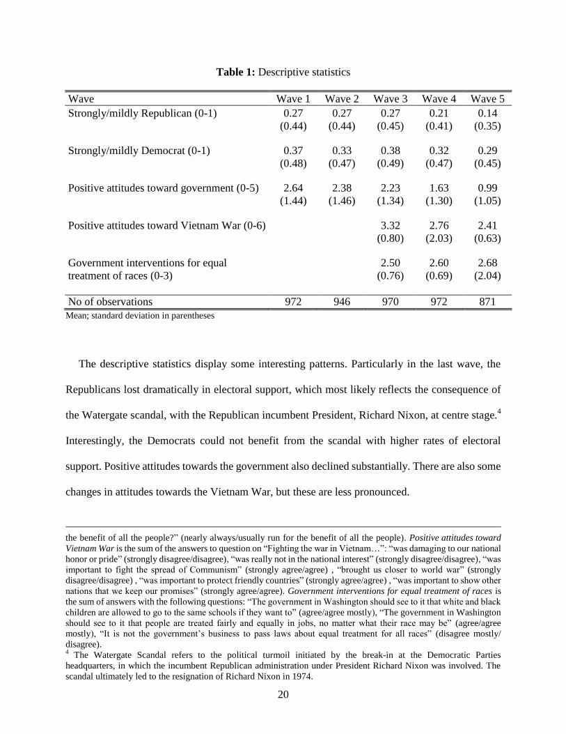
Descriptive statistics for political preferences and attitudes are presented in Table 1. In order to
illustrate our results in a compact form, we present statistics as well as estimation results on indices
which aggregate answers on individual questions to related topics. The composite indices contain
five questions on attitudes towards the government, six questions on attitudes specifically on the
war in Vietnam, and three questions on government interventions for the equal treatment of races.3
The overall picture is not affected by the use of indices rather than the original variables.
2 Available from the Selective Service System: https://www.sss.gov/Portals/0/PDFs/1971.pdf
3 Index components: Positive attitudes toward the government is the sum of answers to the following questions: “Do
you think the government wastes much of the money we pay in taxes?” (little/no), “How much of the time do you
think you can trust the government in Washington to do what is right?” (always/often), “Do you feel that the people
running the government are smart people who usually know what they are doing?” (always/usually know what
doing), “Do you think some of the people running the government are crooked or dishonest?” (hardly any/none),
“Would you say the government is pretty much run for a few big interests looking out for themselves, or is it run for
20
Table 1: Descriptive statistics
Wave Wave 1 Wave 2 Wave 3 Wave 4 Wave 5
Strongly/mildly Republican (0-1) 0.27 0.27 0.27 0.21 0.14
(0.44) (0.44) (0.45) (0.41) (0.35)
Strongly/mildly Democrat (0-1) 0.37 0.33 0.38 0.32 0.29
(0.48) (0.47) (0.49) (0.47) (0.45)
Positive attitudes toward government (0-5) 2.64 2.38 2.23 1.63 0.99
(1.44) (1.46) (1.34) (1.30) (1.05)
Positive attitudes toward Vietnam War (0-6)
3.32 2.76 2.41
(0.80) (2.03) (0.63)
Government interventions for equal
2.50 2.60 2.68
treatment of races (0-3)
(0.76) (0.69) (2.04)
No of observations 972 946 970 972 871
Mean; standard deviation in parentheses
The descriptive statistics display some interesting patterns. Particularly in the last wave, the
Republicans lost dramatically in electoral support, which most likely reflects the consequence of
the Watergate scandal, with the Republican incumbent President, Richard Nixon, at centre stage.4
Interestingly, the Democrats could not benefit from the scandal with higher rates of electoral
support. Positive attitudes towards the government also declined substantially. There are also some
changes in attitudes towards the Vietnam War, but these are less pronounced.
the benefit of all the people?” (nearly always/usually run for the benefit of all the people). Positive attitudes toward
Vietnam War is the sum of the answers to question on “Fighting the war in Vietnam…”: “was damaging to our national
honor or pride” (strongly disagree/disagree), “was really not in the national interest” (strongly disagree/disagree), “was
important to fight the spread of Communism” (strongly agree/agree) , “brought us closer to world war” (strongly
disagree/disagree) , “was important to protect friendly countries” (strongly agree/agree) , “was important to show other
nations that we keep our promises” (strongly agree/agree). Government interventions for equal treatment of races is
the sum of answers with the following questions: “The government in Washington should see to it that white and black
children are allowed to go to the same schools if they want to” (agree/agree mostly), “The government in Washington
should see to it that people are treated fairly and equally in jobs, no matter what their race may be” (agree/agree
mostly), “It is not the government’s business to pass laws about equal treatment for all races” (disagree mostly/
disagree). 4 The Watergate Scandal refers to the political turmoil initiated by the break-in at the Democratic Parties
headquarters, in which the incumbent Republican administration under President Richard Nixon was involved. The
scandal ultimately led to the resignation of Richard Nixon in 1974.
21
A potential problem with this data arises from the fact that we do not observe the exact draft
number for our full sample. The exact day of birth is only provided for respondents who
participated in the fourth wave and did not serve in the military at the time of the interview, which
restricts our estimation sample to 972 individuals (about 70% of our original sample). This
selection, however, is unlikely to be associated with the random draft number (RDN): Young men
born in 1951 were called to report for induction into the military in year 1971. Consequently, no
individual of the initial sample was drafted when the interviews for the fourth wave took place.
Moreover, most individuals were interviewed even before the lottery so that they were not aware of
their draft number and could not have taken any steps to reduce the risk imposed by a small draft
number (such as leaving the country). Therefore, the lottery should be internally valid (exogenous)
for the individuals observed in 1970.
One may worry, however, that attrition from wave 4 to 5 is associated with the draft number,
since we lose a further 10% of our subsample (N =871). Even though individuals who still served
in the military are included, one would expect that dropout rates are highest among those with a
high draft risk due to death on active duty, the inability to locate individuals who are still on active
duty or draft avoidance by leaving the country. Surprisingly, this is not the case. Dropout rates from
wave 4 to 5 are 2 percentage points lower for individuals with lottery numbers below the ceiling
(9% vs. 11%). Nevertheless, attrition from wave 4 to 5 may cause a selection bias. In Table A1 of
the appendix, we provide a balancing test for pre-lottery outcomes for respondents with RDN
below or above the ceiling and who are still observed in wave 5. For all outcomes considered, there
are no striking differences in pre-lottery outcomes between individuals with high and low RDN,
indicating that selection bias is unlikely an issue in this application.
22
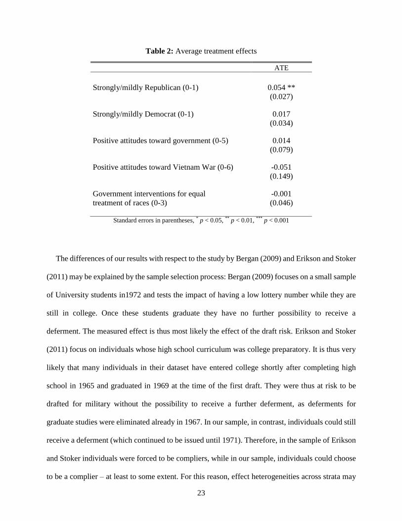
3.2 Average treatment effect
In the following we estimate the effect of a low draft lottery number on political preferences and
Vietnam War attitudes. In the first step we use the experimental estimator to evaluate the ATE.
Table 2 presents the results, where the treatment is a binary indicator that is equal to one if the
random draft number was below the ceiling. Individuals with low draft numbers are about 5% more
likely to report to vote Republican. All other results do not show significant differences between
individuals above and below the cut-off and the estimated coefficients are always very small.
These results are in stark contrast to those of Bergan (2009) and Erikson and Stoker (2011).
Bergan (2009) reports a significantly positive effect of the lottery on the probability of favouring an
immediate withdrawal from Vietnam. Even though our data set contains similar, albeit not exactly
the same measures, we find no significant effect of low lottery numbers on Vietnam War attitudes.
Erikson and Stoker (2011) use a sample of college-bound young males who graduated from high
school in 1965 and were therefore at risk to being drafted in the 1969 lottery since their college
deferment exhausted with graduation. Those males are found to be more likely to report to favour
Democrats over Republicans. Specifically, Erikson and Stoker (2011) show that individuals with
low lottery numbers voted more often for McGovern (Democrat) relative to Nixon (Republican) or
favoured Democratic over Republican attitudes in a rating of attitudes towards McGovern vs.
Nixon, party political activities, a composite issue attitude index, and political ideology showing
preferences for liberal relative to conservative positions. Moreover, individuals with low lottery
numbers expressed more anti-war opinions. In contrast, we find insignificant differences between
individuals with low and high numbers w.r.t. to composite indices on attitudes towards the war and
the government, and the same applies to the specific questions of these indices (not reported).
23
Table 2: Average treatment effects
ATE
Strongly/mildly Republican (0-1) 0.054 **
(0.027)
Strongly/mildly Democrat (0-1) 0.017
(0.034)
Positive attitudes toward government (0-5) 0.014
(0.079)
Positive attitudes toward Vietnam War (0-6) -0.051
(0.149)
Government interventions for equal -0.001
treatment of races (0-3) (0.046)
Standard errors in parentheses, * p < 0.05,
** p < 0.01,
*** p < 0.001
The differences of our results with respect to the study by Bergan (2009) and Erikson and Stoker
(2011) may be explained by the sample selection process: Bergan (2009) focuses on a small sample
of University students in1972 and tests the impact of having a low lottery number while they are
still in college. Once these students graduate they have no further possibility to receive a
deferment. The measured effect is thus most likely the effect of the draft risk. Erikson and Stoker
(2011) focus on individuals whose high school curriculum was college preparatory. It is thus very
likely that many individuals in their dataset have entered college shortly after completing high
school in 1965 and graduated in 1969 at the time of the first draft. They were thus at risk to be
drafted for military without the possibility to receive a further deferment, as deferments for
graduate studies were eliminated already in 1967. In our sample, in contrast, individuals could still
receive a deferment (which continued to be issued until 1971). Therefore, in the sample of Erikson
and Stoker individuals were forced to be compliers, while in our sample, individuals could choose
to be a complier – at least to some extent. For this reason, effect heterogeneities across strata may
24
be important. In the following we distinguish between different strata and estimate direct and
indirect effects of the draft lottery.
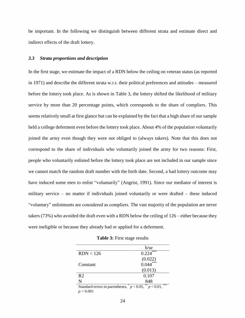
3.3 Strata proportions and description
In the first stage, we estimate the impact of a RDN below the ceiling on veteran status (as reported
in 1971) and describe the different strata w.r.t. their political preferences and attitudes – measured
before the lottery took place. As is shown in Table 3, the lottery shifted the likelihood of military
service by more than 20 percentage points, which corresponds to the share of compliers. This
seems relatively small at first glance but can be explained by the fact that a high share of our sample
held a college deferment even before the lottery took place. About 4% of the population voluntarily
joined the army even though they were not obliged to (always takers). Note that this does not
correspond to the share of individuals who voluntarily joined the army for two reasons: First,
people who voluntarily enlisted before the lottery took place are not included in our sample since
we cannot match the random draft number with the birth date. Second, a bad lottery outcome may
have induced some men to enlist “voluntarily” (Angrist, 1991). Since our mediator of interest is
military service – no matter if individuals joined voluntarily or were drafted – these induced
“voluntary” enlistments are considered as compliers. The vast majority of the population are never
takers (73%) who avoided the draft even with a RDN below the ceiling of 126 – either because they
were ineligible or because they already had or applied for a deferment.
Table 3: First stage results
b/se
RDN < 126 0.224***
(0.022)
Constant 0.044***
(0.013)
R2 0.107
N 848 Standard errors in parentheses,
* p < 0.05,
** p < 0.01,
***
p < 0.001
25
Table 4: Mean differences across strata (pre-treatment characteristics)
C vs. AT
(T=0)
C vs. NT
(T=0)
Wave 3: Military knowledge test (0-40) 0.862 1.143
(1.31) (1.519)
Wave 1: IQ Test -6.254** -8.794**
(3.548) (3.761)
Wave 1: Self perceived intelligence 0.223** 0.497
(1: top 10% to 6: bottom 10%) (0.207) (0.305)
Wave 1: Has college plans -0.064 -0.345**
(0.139) (0.157)
Military classification (Wave 4)
Student deferment -0.072 -0.386**
(0.14) (0.171)
Available for military 0.140** 0.461***
(0.137) (0.142)
Not classified -0.004 0.019
(0.057) (0.066)
Other -0.064 -0.094
(0.105) (0.122)
Standard errors in parentheses, * p < 0.05,
** p < 0.01,
*** p < 0.001
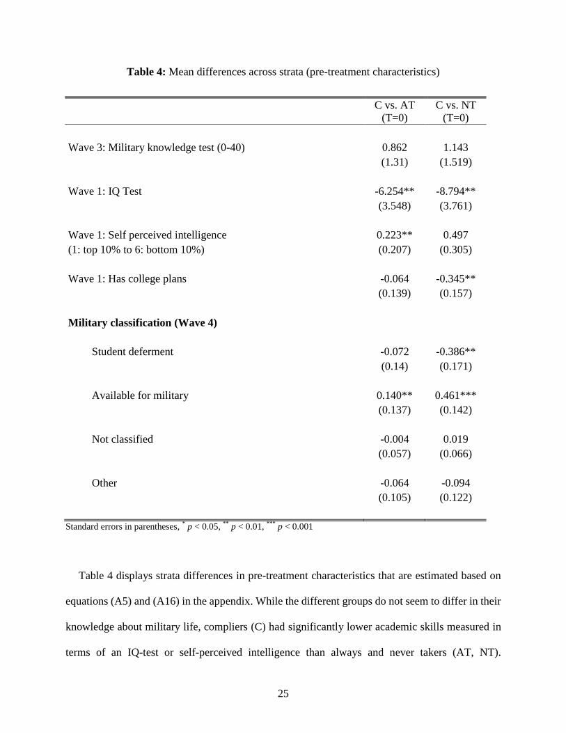
Table 4 displays strata differences in pre-treatment characteristics that are estimated based on
equations (A5) and (A16) in the appendix. While the different groups do not seem to differ in their
knowledge about military life, compliers (C) had significantly lower academic skills measured in
terms of an IQ-test or self-perceived intelligence than always and never takers (AT, NT).
26
Compliers were also significantly less likely than never takers to have college plans or to hold a
student deferment shortly before or at the draft lottery, and more likely available for the military.
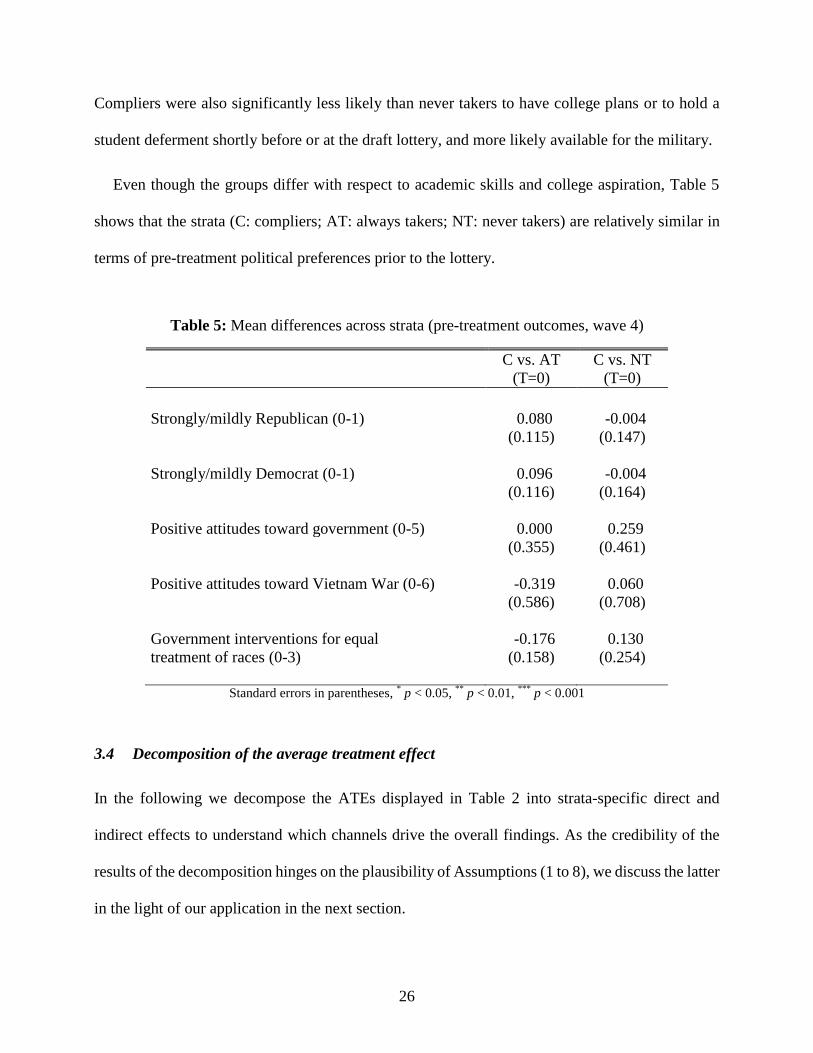
Even though the groups differ with respect to academic skills and college aspiration, Table 5
shows that the strata (C: compliers; AT: always takers; NT: never takers) are relatively similar in
terms of pre-treatment political preferences prior to the lottery.
Table 5: Mean differences across strata (pre-treatment outcomes, wave 4)
C vs. AT
(T=0)
C vs. NT
(T=0)
Strongly/mildly Republican (0-1) 0.080 -0.004
(0.115) (0.147)
Strongly/mildly Democrat (0-1) 0.096 -0.004
(0.116) (0.164)
Positive attitudes toward government (0-5) 0.000 0.259
(0.355) (0.461)
Positive attitudes toward Vietnam War (0-6) -0.319 0.060
(0.586) (0.708)
Government interventions for equal -0.176 0.130
treatment of races (0-3) (0.158) (0.254)
Standard errors in parentheses,
* p < 0.05,
** p < 0.01,
*** p < 0.001
3.4 Decomposition of the average treatment effect
In the following we decompose the ATEs displayed in Table 2 into strata-specific direct and
indirect effects to understand which channels drive the overall findings. As the credibility of the
results of the decomposition hinges on the plausibility of Assumptions (1 to 8), we discuss the latter
in the light of our application in the next section.
27
3.4.1 Plausibility of the identifying assumptions
Assumption 1 implies that there are no confounders jointly affecting the lottery outcome on the one
hand and military service and/or the outcome variables on the other hand. This assumption seems
uncontroversial since the draft number was randomized and unlike the first lottery that had taken
place in 1969, the randomization was well executed (Fienberg, 1971). Also balancing tests with
respect to pre-treatment outcomes measured in wave 4 (Table A1) support this assumption.
Assumption 2 rules out the existence of defiers, which seems plausible in the context of the draft
lottery. It appears hard to argue why an individual should avoid the draft when being chosen by the
lottery, but voluntarily join the army when not being chosen. Assumption 3 rules out anticipation
effects of the treatment or the mediator w.r.t. to the outcome in the baseline period. Given the fact
that the results of the lottery could not have been foreseen and that the large majority of interviews
took place before the lottery, this assumption is also likely satisfied and supported by the results of
the balancing test with respect to outcomes measured in wave 4.
Assumption 4 imposes common trends for compliers and never takers when receiving a high
lottery number and not joining the army. This is a fairly standard restriction in the DiD literature,
arguing that the mean outcomes of various groups develop in a comparable way if no one receives
any treatment. The fact that compliers and never taker had fairly similar outcomes prior the lottery
(see Table 5) somewhat supports this assumption, albeit similarity in levels is strictly speaking
neither necessary nor sufficient for common trends. Assumption 1 to 4 are sufficient to estimate the
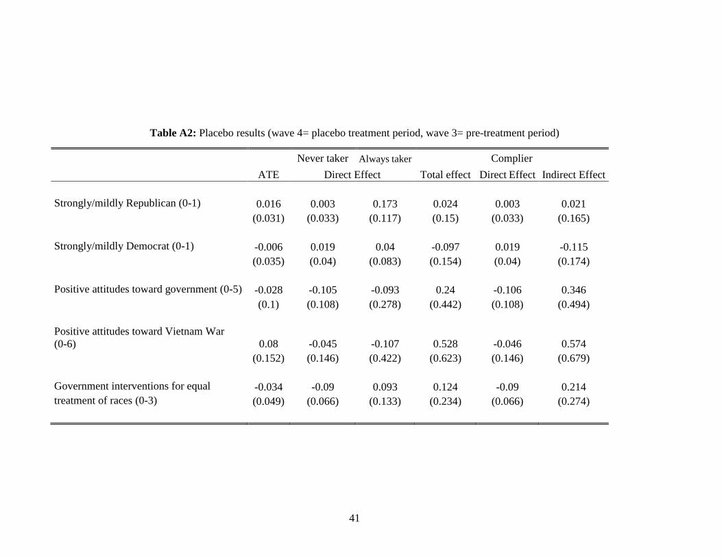
direct effect on the never takers. We perform placebo estimations by using wave 4 as the placebo
follow up period and wave 3 as baseline period (Table A2). The placebo effects for the direct effect
on the never takers are small and insignificant for all outcomes and therefore support our strategy.
Assumption 5 would be satisfied if the joint average effect of the lottery and military service
was comparable across individuals voluntarily joining the army (always takers) or being induced to
28
join (compliers), which seems to be a very strong assumption. Alternatively, one may assume a
zero direct effect on always takers (Assumption 6). This seems more credible in our current setting:
Always takers are not forced to change their behavior because they would join the army anyway
such that a low lottery number per se should have no direct effect on political preferences. Under
Assumptions 1, 2, 3, 4, and 6, we can consistently estimate the total treatment effect on the
compliers. We also perform placebo estimations of the total treatment effect on compliers (Table
A2). Results are small and insignificant.
Assumption 7 imposes common trends for compliers and never takers when both groups receive
low lottery numbers but neither group actually joins the army. This means that outcomes of
compliers and never takers would develop in a similar way if one could induce compliers to react to
the lottery in a similar way as never takers. Combined with previous assumptions this implies that
the direct effects of the lottery when neither group joins the army are homogeneous. Assumption 8,
in contrast, assumes common trends for compliers and always takers when both groups receive
high lottery numbers but join the army anyway. Note that Assumptions 7 and 8 (in combination
with other assumptions) identify different indirect effects: Assumption 7 gives the effect of joining
the army among compliers when having a low random number (𝑧 = 1). Assumption 8, in contrast,
identifies the effect of joining the army when compliers receive a high random number (𝑧 = 0).
This seems to be a hypothetical effect since compliers do not join the army if they are not induced
to by the lottery. We therefore impose Assumption 7 in our analysis and also consider placebo
estimations (Table A2) that yield small and insignificant results. Note that in the absence of any
direct effect of the lottery, the indirect effects under Assumptions 7 and 8 are identical and
correspond to the LATE.
29
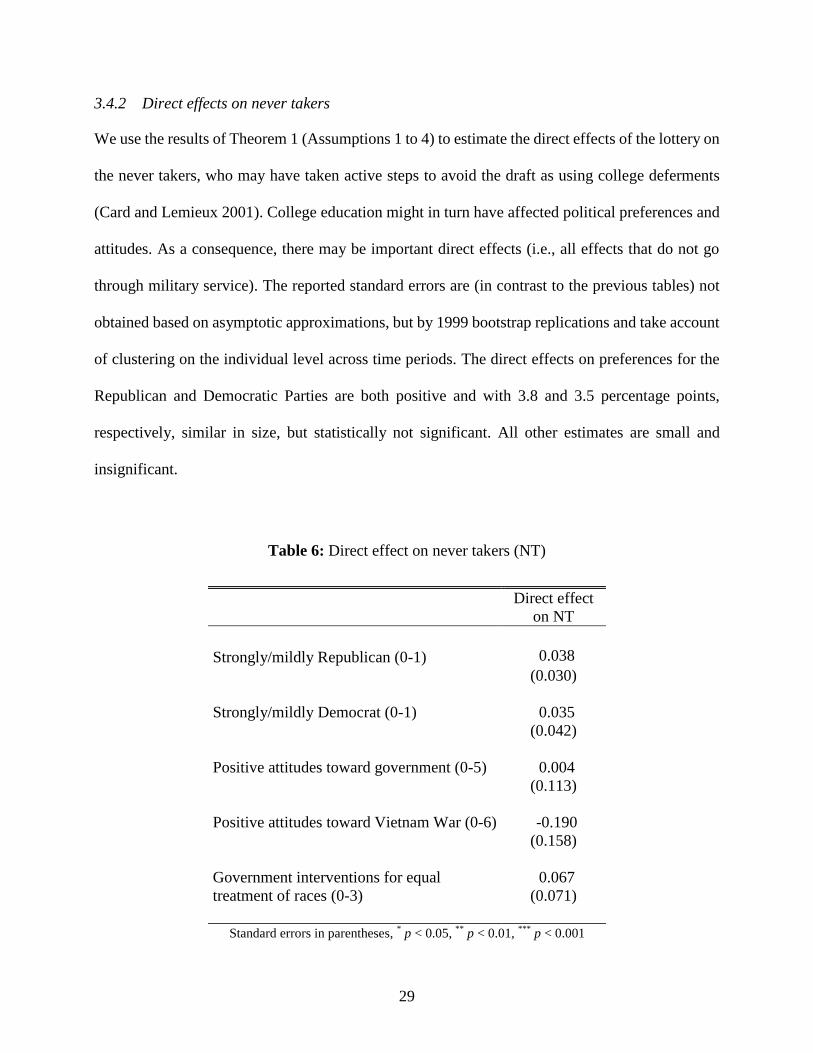
3.4.2 Direct effects on never takers
We use the results of Theorem 1 (Assumptions 1 to 4) to estimate the direct effects of the lottery on
the never takers, who may have taken active steps to avoid the draft as using college deferments
(Card and Lemieux 2001). College education might in turn have affected political preferences and
attitudes. As a consequence, there may be important direct effects (i.e., all effects that do not go
through military service). The reported standard errors are (in contrast to the previous tables) not
obtained based on asymptotic approximations, but by 1999 bootstrap replications and take account
of clustering on the individual level across time periods. The direct effects on preferences for the
Republican and Democratic Parties are both positive and with 3.8 and 3.5 percentage points,
respectively, similar in size, but statistically not significant. All other estimates are small and
insignificant.
Table 6: Direct effect on never takers (NT)
Direct effect
on NT
Strongly/mildly Republican (0-1) 0.038
(0.030)
Strongly/mildly Democrat (0-1) 0.035
(0.042)
Positive attitudes toward government (0-5) 0.004
(0.113)
Positive attitudes toward Vietnam War (0-6) -0.190
(0.158)
Government interventions for equal 0.067
treatment of races (0-3) (0.071)
Standard errors in parentheses, * p < 0.05,
** p < 0.01,
*** p < 0.001
30
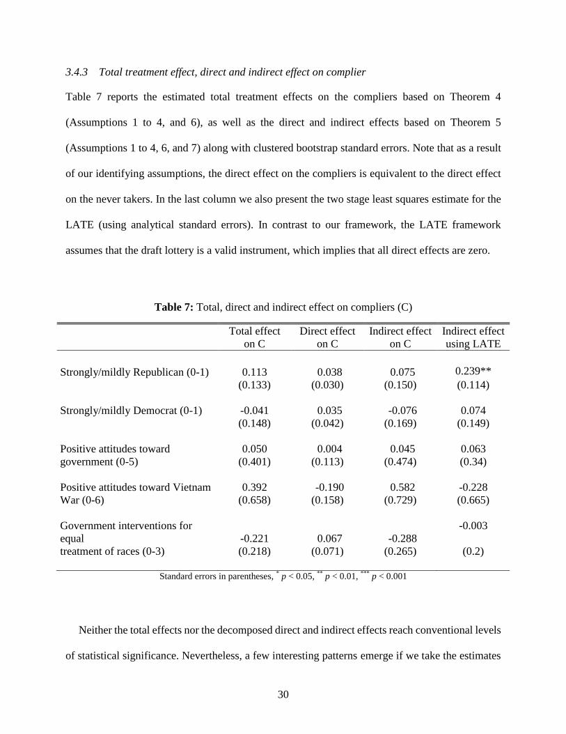
3.4.3 Total treatment effect, direct and indirect effect on complier
Table 7 reports the estimated total treatment effects on the compliers based on Theorem 4
(Assumptions 1 to 4, and 6), as well as the direct and indirect effects based on Theorem 5
(Assumptions 1 to 4, 6, and 7) along with clustered bootstrap standard errors. Note that as a result
of our identifying assumptions, the direct effect on the compliers is equivalent to the direct effect
on the never takers. In the last column we also present the two stage least squares estimate for the
LATE (using analytical standard errors). In contrast to our framework, the LATE framework
assumes that the draft lottery is a valid instrument, which implies that all direct effects are zero.
Table 7: Total, direct and indirect effect on compliers (C)
Total effect
on C
Direct effect
on C
Indirect effect
on C
Indirect effect
using LATE
Strongly/mildly Republican (0-1) 0.113 0.038 0.075 0.239**
(0.133) (0.030) (0.150) (0.114)
Strongly/mildly Democrat (0-1) -0.041 0.035 -0.076 0.074
(0.148) (0.042) (0.169) (0.149)
Positive attitudes toward 0.050 0.004 0.045 0.063
government (0-5) (0.401) (0.113) (0.474) (0.34)
Positive attitudes toward Vietnam 0.392 -0.190 0.582 -0.228
War (0-6) (0.658) (0.158) (0.729) (0.665)
Government interventions for
equal -0.221 0.067 -0.288
-0.003
treatment of races (0-3) (0.218) (0.071) (0.265) (0.2)
Standard errors in parentheses,
* p < 0.05,
** p < 0.01,
*** p < 0.001
Neither the total effects nor the decomposed direct and indirect effects reach conventional levels
of statistical significance. Nevertheless, a few interesting patterns emerge if we take the estimates
31
at face value. The total effects on compliers’ party preferences, characterized by an increase in the
support for the Republican Party and a decrease in the support for the Democrats, appears to be
mainly driven by the indirect effect of the draft lottery which goes through military service.
However, both the total and the indirect effects on compliers are far smaller than the LATE
estimate, which suggests that military service increases support for the Republican Party by 24
percentage points and is significant at the 5% level. This points to the non-robustness of the results
across various econometric approaches, as the true LATE equals the true indirect effect among
compliers in the absence of direct effects. We therefore argue that previous studies that use the
lottery as instrument for military service should be interpreted with caution.
4 Conclusion
We propose a difference-in-differences approach to disentangle the total causal effect of a policy
intervention into a direct effect and an indirect effect operating through a binary intermediate
variable (or mediator) within subpopulations (or strata). The strata are defined upon how the
mediator reacts to the treatment. We show under which assumptions the direct effects on the
always and never takers (whose mediator is not affected by the treatment) as well as the direct and
indirect effects on the compliers (whose mediator reacts to the treatment) are identified.
We apply our method to investigate the effect of the Vietnam draft lottery between 1969 and
1972 in the US on political preferences as well as personal views on the government and war
policies. Our mediator of interest is military service during the Vietnam War. A subgroup of
individuals (compliers) was induced by the lottery to serve in the army, while others avoided the
draft (never takers) or would have served in any case (always takers). In a first step, we estimate the
average treatment effect in the total population and find a roughly 5 percentage points higher
probability of voting for the Republican Party (and insignificant effects on other outcomes). In a
32
second step, we estimate the direct and indirect effects of the draft lottery within subgroups. In
general, we do not find statistically significant effects, even though several of the total and indirect
effects on the compliers are sizeable in magnitude, which suggests that the compliers drive the
overall results. It therefore seems that if anything, compliers serving in Vietnam are less affected
by the overall decline in Republican support supposedly due to the unravelling of the Watergate
Scandal. At the same time, both the total and indirect estimates of voting for the Republican Party
among compliers are considerably smaller than the two stage least squares estimate, which uses the
lottery as an instrument for military service. This non-robustness of results across methods casts
doubts on the instrument validity of the draft lottery and in particular the satisfaction of the
exclusion restriction that has been frequently imposed in the literature.
33
Appendix
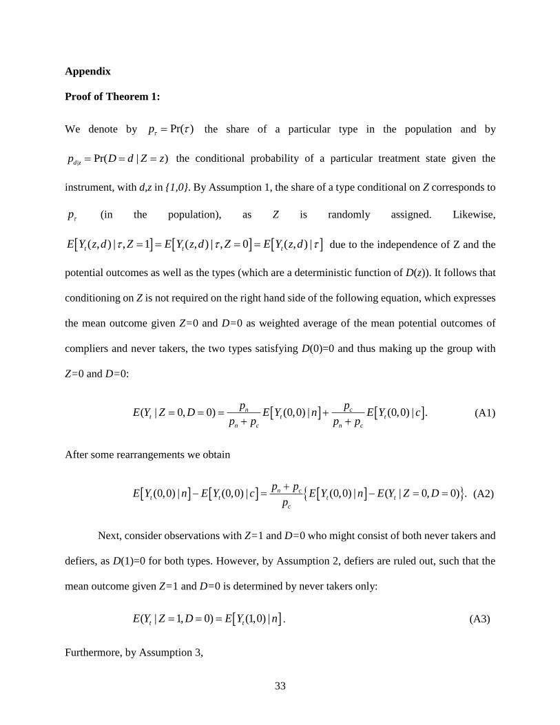
Proof of Theorem 1:
We denote by Pr( )p the share of a particular type in the population and by
| Pr( | )d zp D d Z z the conditional probability of a particular treatment state given the
instrument, with d,z in {1,0}. By Assumption 1, the share of a type conditional on Z corresponds to
p (in the population), as Z is randomly assigned. Likewise,
( , ) | , 1 ( , ) | , 0 ( , ) |t t tE Y z d Z E Y z d Z E Y z d due to the independence of Z and the
potential outcomes as well as the types (which are a deterministic function of D(z)). It follows that
conditioning on Z is not required on the right hand side of the following equation, which expresses
the mean outcome given Z=0 and D=0 as weighted average of the mean potential outcomes of
compliers and never takers, the two types satisfying D(0)=0 and thus making up the group with
Z=0 and D=0:
( | 0, 0) (0,0) | (0,0) | .n ct t t
n c n c
p pE Y Z D E Y n E Y c
p p p p
(A1)
After some rearrangements we obtain
(0,0) | (0,0) | (0,0) | ( | 0, 0) .n ct t t t
c
p pE Y n E Y c E Y n E Y Z D
p
(A2)
Next, consider observations with Z=1 and D=0 who might consist of both never takers and
defiers, as D(1)=0 for both types. However, by Assumption 2, defiers are ruled out, such that the
mean outcome given Z=1 and D=0 is determined by never takers only:
( | 1, 0) (1,0) |t tE Y Z D E Y n . (A3)
Furthermore, by Assumption 3,
34
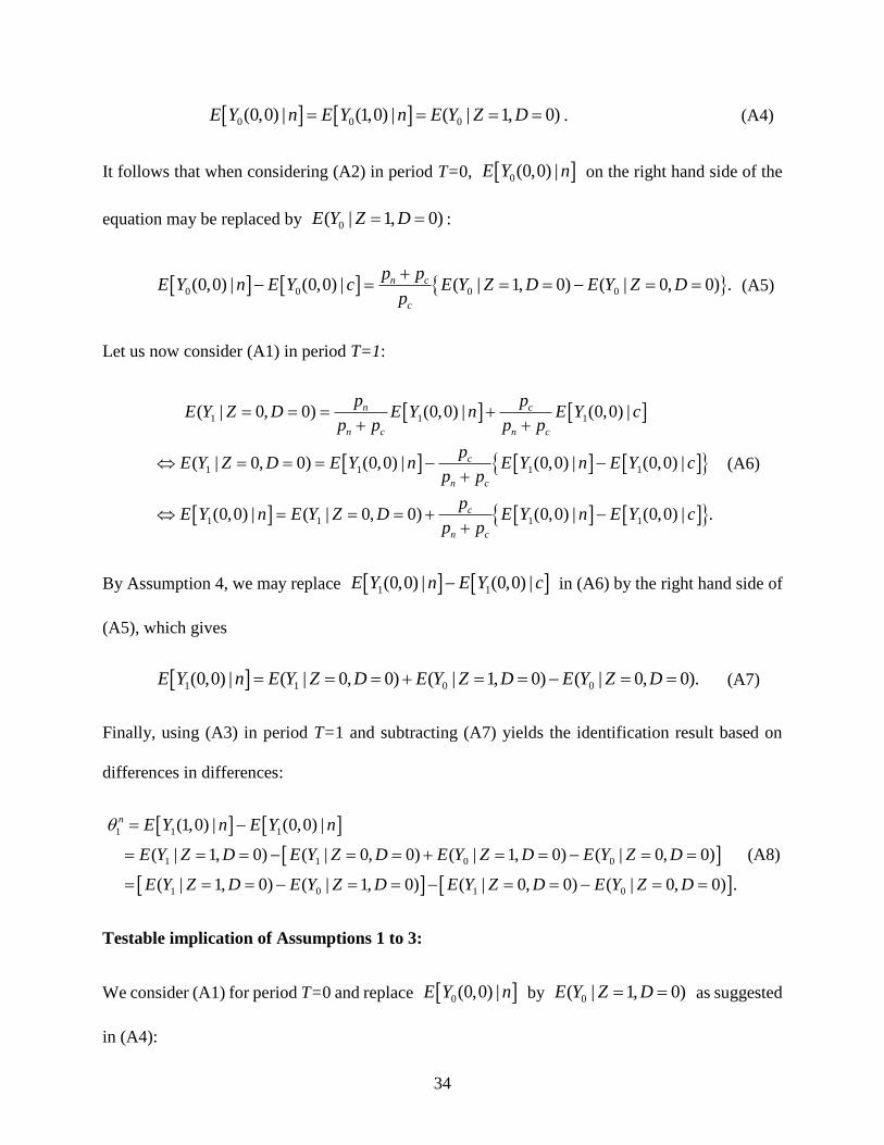
0 0 0(0,0) | (1,0) | ( | 1, 0)E Y n E Y n E Y Z D . (A4)
It follows that when considering (A2) in period T=0, 0(0,0) |E Y n on the right hand side of the
equation may be replaced by 0( | 1, 0)E Y Z D :
0 0 0 0(0,0) | (0,0) | ( | 1, 0) ( | 0, 0) .n c
c
p pE Y n E Y c E Y Z D E Y Z D
p
(A5)
Let us now consider (A1) in period T=1:
1 1 1
1 1 1 1
1 1 1 1
( | 0, 0) (0,0) | (0,0) |
( | 0, 0) (0,0) | (0,0) | (0,0) |
(0,0) | ( | 0, 0) (0,0) | (0,0) | .
n c
n c n c
c
n c
c
n c
p pE Y Z D E Y n E Y c
p p p p
pE Y Z D E Y n E Y n E Y c
p p
pE Y n E Y Z D E Y n E Y c
p p
(A6)
By Assumption 4, we may replace 1 1(0,0) | (0,0) |E Y n E Y c in (A6) by the right hand side of
(A5), which gives
1 1 0 0(0,0) | ( | 0, 0) ( | 1, 0) ( | 0, 0).E Y n E Y Z D E Y Z D E Y Z D (A7)
Finally, using (A3) in period T=1 and subtracting (A7) yields the identification result based on
differences in differences:
1 1 1
1 1 0 0
1 0 1 0
(1,0) | (0,0) |
( | 1, 0) ( | 0, 0) ( | 1, 0) ( | 0, 0)
( | 1, 0) ( | 1, 0) ( | 0, 0) ( | 0, 0) .
n E Y n E Y n
E Y Z D E Y Z D E Y Z D E Y Z D
E Y Z D E Y Z D E Y Z D E Y Z D
(A8)
Testable implication of Assumptions 1 to 3:
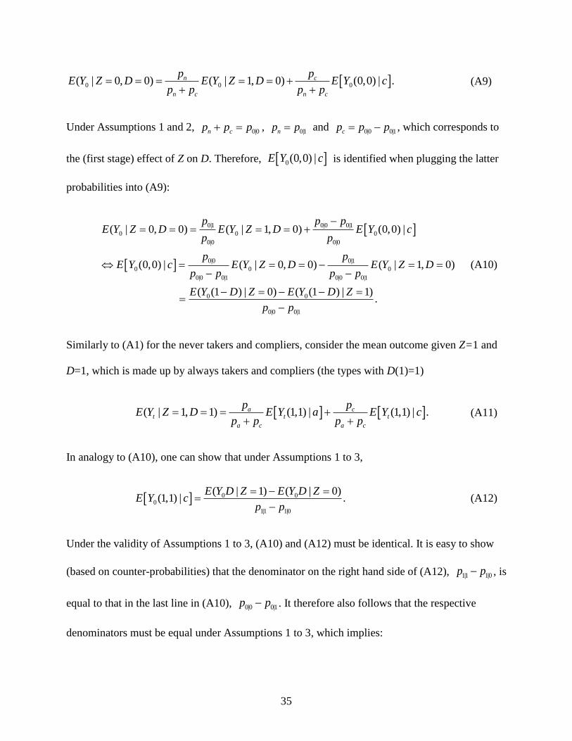
We consider (A1) for period T=0 and replace 0(0,0) |E Y n by 0( | 1, 0)E Y Z D as suggested
in (A4):
35
0 0 0( | 0, 0) ( | 1, 0) (0,0) | .n c
n c n c
p pE Y Z D E Y Z D E Y c
p p p p
(A9)
Under Assumptions 1 and 2, 0|0n cp p p , 0|1np p and 0|0 0|1cp p p , which corresponds to
the (first stage) effect of Z on D. Therefore, 0(0,0) |E Y c is identified when plugging the latter
probabilities into (A9):
0|1 0|0 0|1
0 0 0
0|0 0|0
0|0 0|1
0 0 0
0|0 0|1 0|0 0|1
0 0
0|0 0|1
( | 0, 0) ( | 1, 0) (0,0) |
(0,0) | ( | 0, 0) ( | 1, 0)
( (1 ) | 0) ( (1 ) | 1).
p p pE Y Z D E Y Z D E Y c
p p
p pE Y c E Y Z D E Y Z D
p p p p
E Y D Z E Y D Z
p p
(A10)
Similarly to (A1) for the never takers and compliers, consider the mean outcome given Z=1 and
D=1, which is made up by always takers and compliers (the types with D(1)=1)
( | 1, 1) (1,1) | (1,1) | .a ct t t
a c a c
p pE Y Z D E Y a E Y c
p p p p
(A11)
In analogy to (A10), one can show that under Assumptions 1 to 3,
0 00
1|1 1|0
( | 1) ( | 0)(1,1) | .
E Y D Z E Y D ZE Y c
p p
(A12)
Under the validity of Assumptions 1 to 3, (A10) and (A12) must be identical. It is easy to show
(based on counter-probabilities) that the denominator on the right hand side of (A12), 1|1 1|0p p , is
equal to that in the last line in (A10), 0|0 0|1p p . It therefore also follows that the respective
denominators must be equal under Assumptions 1 to 3, which implies:
36
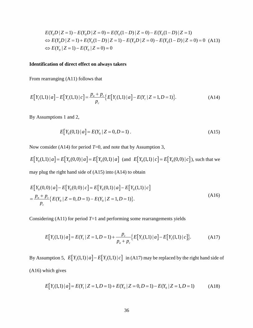
0 0 0 0
0 0 0 0
0 0
( | 1) ( | 0) ( (1 ) | 0) ( (1 ) | 1)
( | 1) ( (1 ) | 1) ( | 0) ( (1 ) | 0) 0
( | 1) ( | 0) 0
E Y D Z E Y D Z E Y D Z E Y D Z
E Y D Z E Y D Z E Y D Z E Y D Z
E Y Z E Y Z
(A13)
Identification of direct effect on always takers
From rearranging (A11) follows that
(1,1) | (1,1) | (1,1) | ( | 1, 1) .a ct t t t
c
p pE Y a E Y c E Y a E Y Z D
p
(A14)
By Assumptions 1 and 2,
0 0(0,1) | ( | 0, 1)E Y a E Y Z D . (A15)
Now consider (A14) for period T=0, and note that by Assumption 3,
0 0 0(1,1) | (0,0) | (0,1) |E Y a E Y a E Y a (and 0 0(1,1) | (0,0) |E Y c E Y c ), such that we
may plug the right hand side of (A15) into (A14) to obtain
0 0 0 0
0 0
(0,0) | (0,0) | (0,1) | (1,1) |
( | 0, 1) ( | 1, 1) .a c
c
E Y a E Y c E Y a E Y c
p pE Y Z D E Y Z D
p
(A16)
Considering (A11) for period T=1 and performing some rearrangements yields
1 1 1 1(1,1) | ( | 1, 1) (1,1) | (1,1) | .c
a c
pE Y a E Y Z D E Y a E Y c
p p
(A17)
By Assumption 5, 1 1(1,1) | (1,1) |E Y a E Y c in (A17) may be replaced by the right hand side of
(A16) which gives
1 1 0 0(1,1) | ( | 1, 1) ( | 0, 1) ( | 1, 1)E Y a E Y Z D E Y Z D E Y Z D (A18)
37
Finally, acknowledging that 1 1(0,1) | ( | 0, 1)E Y a E Y Z D by Assumptions 1 and 2 and
subtracting (A18) yields the identification result based on differences in differences:
1 1 1
1 0 0 1
1 0 1 0
(1,1) | (0,1) |
( | 1, 1) ( | 0, 1) ( | 1, 1) ( | 0, 1)
( | 1, 1) ( | 1, 1) ( | 0, 1) ( | 0, 1) .
a E Y a E Y a
E Y Z D E Y Z D E Y Z D E Y Z D
E Y Z D E Y Z D E Y Z D E Y Z D
(A19)
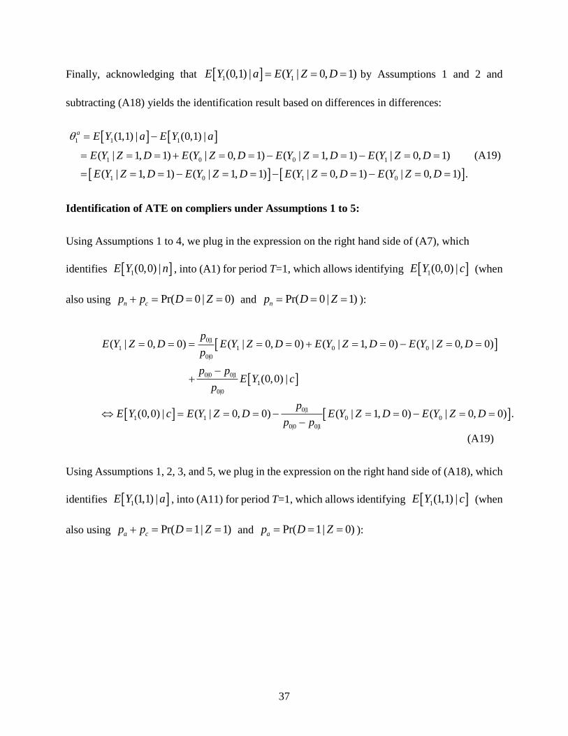
Identification of ATE on compliers under Assumptions 1 to 5:
Using Assumptions 1 to 4, we plug in the expression on the right hand side of (A7), which
identifies 1(0,0) |E Y n , into (A1) for period T=1, which allows identifying 1(0,0) |E Y c (when
also using Pr( 0 | 0)n cp p D Z and Pr( 0 | 1)np D Z ):
0|1
1 1 0 0
0|0
0|0 0|1
1
0|0
0|1
1 1 0 0
0|0 0|1
( | 0, 0) ( | 0, 0) ( | 1, 0) ( | 0, 0)
(0,0) |
(0,0) | ( | 0, 0) ( | 1, 0) ( | 0, 0) .
pE Y Z D E Y Z D E Y Z D E Y Z D
p
p pE Y c
p
pE Y c E Y Z D E Y Z D E Y Z D
p p
(A19)
Using Assumptions 1, 2, 3, and 5, we plug in the expression on the right hand side of (A18), which
identifies 1(1,1) |E Y a , into (A11) for period T=1, which allows identifying 1(1,1) |E Y c (when
also using Pr( 1| 1)a cp p D Z and Pr( 1| 0)ap D Z ):
38
1|0
1 1 0 0
1|1
1|1 1|0
1
1|1
1|0
1 1 0 0
1|1 1|0
( | 1, 1) ( | 1, 1) ( | 0, 1) ( | 1, 1)
(1,1) |
(1,1) | ( | 1, 1) ( | 0, 1) ( | 1, 1) .
pE Y Z D E Y Z D E Y Z D E Y Z D
p
p pE Y c
p
pE Y c E Y Z D E Y Z D E Y Z D
p p
(A20)
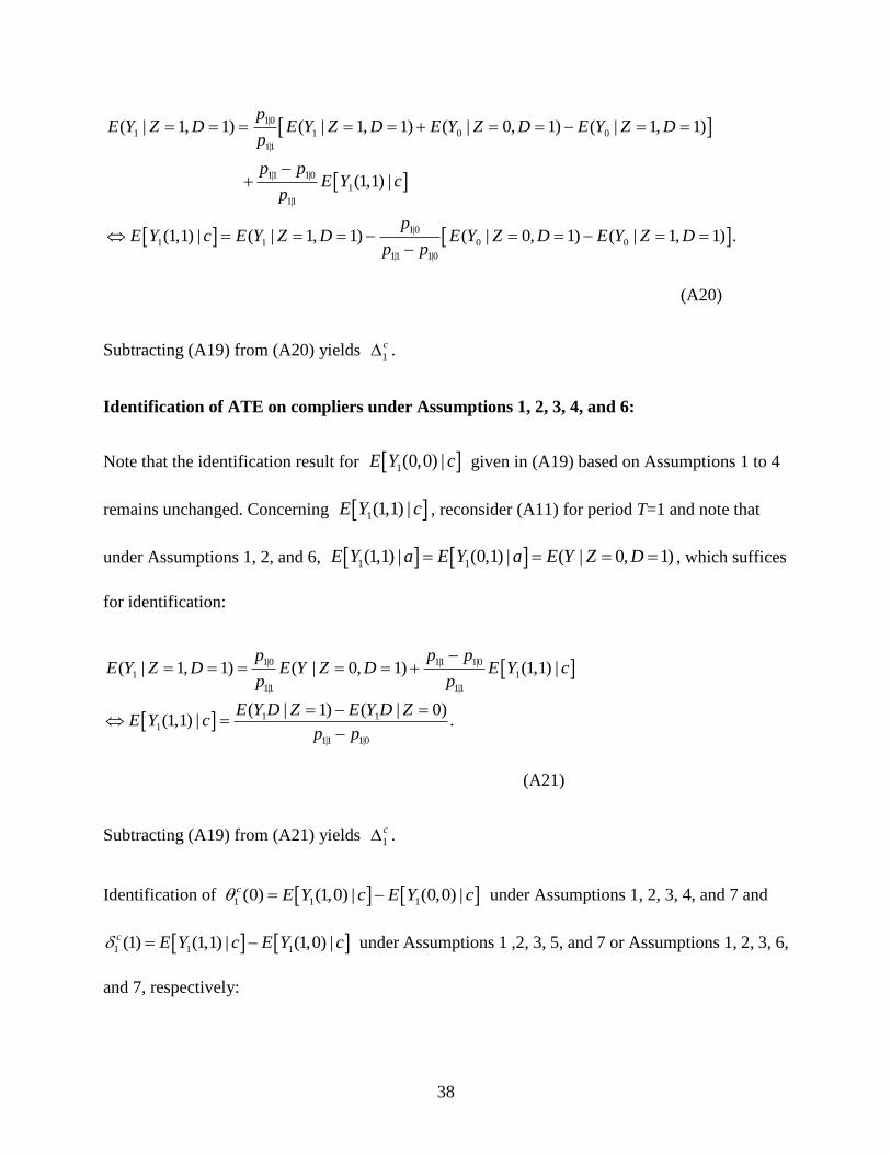
Subtracting (A19) from (A20) yields 1
c .
Identification of ATE on compliers under Assumptions 1, 2, 3, 4, and 6:
Note that the identification result for 1(0,0) |E Y c given in (A19) based on Assumptions 1 to 4
remains unchanged. Concerning 1(1,1) |E Y c , reconsider (A11) for period T=1 and note that
under Assumptions 1, 2, and 6, 1 1(1,1) | (0,1) | ( | 0, 1)E Y a E Y a E Y Z D , which suffices
for identification:
1|0 1|1 1|0
1 1
1|1 1|1
1 11
1|1 1|0
( | 1, 1) ( | 0, 1) (1,1) |
( | 1) ( | 0)(1,1) | .
p p pE Y Z D E Y Z D E Y c
p p
E Y D Z E Y D ZE Y c
p p
(A21)
Subtracting (A19) from (A21) yields 1
c .
Identification of 1 1 1(0) (1,0) | (0,0) |c E Y c E Y c under Assumptions 1, 2, 3, 4, and 7 and
1 1 1(1) (1,1) | (1,0) |c E Y c E Y c under Assumptions 1 ,2, 3, 5, and 7 or Assumptions 1, 2, 3, 6,
and 7, respectively:
39
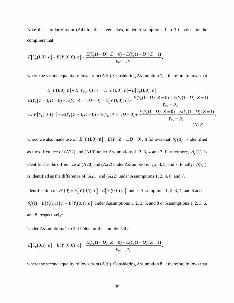
Note that similarly as in (A4) for the never takes, under Assumptions 1 to 3 it holds for the
compliers that
0 00 0
0|0 0|1
( (1 ) | 0) ( (1 ) | 1)(1,0) | (0,0) | ,
E Y D Z E Y D ZE Y c E Y c
p p
where the second equality follows from (A10). Considering Assumption 7, it therefore follows that
1 0 1 0
0 01 0 1
0|0 0|1
0 01 1 0
0|0 0|1
(1,0) | (1,0) | (1,0) | (1,0) |
( (1 ) | 0) ( (1 ) | 1)( | 1, 0) ( | 1, 0) (1,0) |
( (1 ) | 0) ( (1 ) | 1)(1,0) | ( | 1, 0) ( | 1, 0) ,
E Y n E Y n E Y c E Y c
E Y D Z E Y D ZE Y Z D E Y Z D E Y c
p p
E Y D Z E Y D ZE Y c E Y Z D E Y Z D
p p
(A22)
where we also made use of (1,0) | ( | 1, 0)t tE Y n E Y Z D . It follows that 1 (0)c is identified
as the difference of (A22) and (A19) under Assumptions 1, 2, 3, 4 and 7. Furthermore, 1 (1)c is
identified as the difference of (A20) and (A22) under Assumptions 1, 2, 3, 5, and 7. Finally, 1 (1)c
is identified as the difference of (A21) and (A22) under Assumptions 1, 2, 3, 6, and 7.
Identification of 1 1 1(0) (0,1) | (0,0) |c E Y c E Y c under Assumptions 1, 2, 3, 4, and 8 and
1 1 1(1) (1,1) | (0,1) |c E Y c E Y c under Assumptions 1, 2, 3, 5, and 8 or Assumptions 1, 2, 3, 6,
and 8, respectively:
Under Assumptions 1 to 3 it holds for the compliers that
0 00 0
0|0 0|1
( (1 ) | 0) ( (1 ) | 1)(0,1) | (0,0) | ,
E Y D Z E Y D ZE Y c E Y c
p p
where the second equality follows from (A10). Considering Assumption 8, it therefore follows that
40
1 0 1 0
0 01 0 1
0|0 0|1
0 01 1 0
0|0 0|1
(0,1) | (0,1) | (0,1) | (0,1) |
( (1 ) | 0) ( (1 ) | 1)( | 0, 1) ( | 0, 1) (0,1) |
( (1 ) | 0) ( (1 ) | 1)(0,1) | ( | 0, 1) ( | 0, 1) ,
E Y a E Y a E Y c E Y c
E Y D Z E Y D ZE Y Z D E Y Z D E Y c
p p
E Y D Z E Y D ZE Y c E Y Z D E Y Z D
p p
(A23)
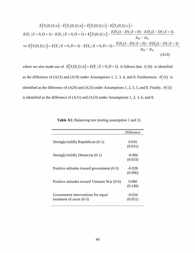
where we also made use of (0,1) | ( | 0, 1)t tE Y a E Y Z D . It follows that 1 (0)c is identified
as the difference of (A23) and (A19) under Assumptions 1, 2, 3, 4, and 8. Furthermore, 1 (1)c is
identified as the difference of (A20) and (A23) under Assumptions 1, 2, 3, 5, and 8. Finally, 1 (1)c
is identified as the difference of (A21) and (A23) under Assumptions 1, 2, 3, 6, and 8.
Table A1: Balancing test (testing assumption 1 and 3)
Difference
Strongly/mildly Republican (0-1) 0.016
(0.031)
Strongly/mildly Democrat (0-1) -0.006
(0.033)
Positive attitudes toward government (0-5) -0.028
(0.096)
Positive attitudes toward Vietnam War (0-6) 0.080
(0.149)
Government interventions for equal -0.034
treatment of races (0-3) (0.051)
41
Table A2: Placebo results (wave 4= placebo treatment period, wave 3= pre-treatment period)
ATE
Never taker Always taker Complier
Direct Effect Total effect Direct Effect Indirect Effect
Strongly/mildly Republican (0-1) 0.016 0.003 0.173 0.024 0.003 0.021
(0.031) (0.033) (0.117) (0.15) (0.033) (0.165)
Strongly/mildly Democrat (0-1) -0.006 0.019 0.04 -0.097 0.019 -0.115
(0.035) (0.04) (0.083) (0.154) (0.04) (0.174)
Positive attitudes toward government (0-5) -0.028 -0.105 -0.093 0.24 -0.106 0.346
(0.1) (0.108) (0.278) (0.442) (0.108) (0.494)
Positive attitudes toward Vietnam War
(0-6) 0.08 -0.045 -0.107 0.528 -0.046 0.574
(0.152) (0.146) (0.422) (0.623) (0.146) (0.679)
Government interventions for equal -0.034 -0.09 0.093 0.124 -0.09 0.214
treatment of races (0-3) (0.049) (0.066) (0.133) (0.234) (0.066) (0.274)
42
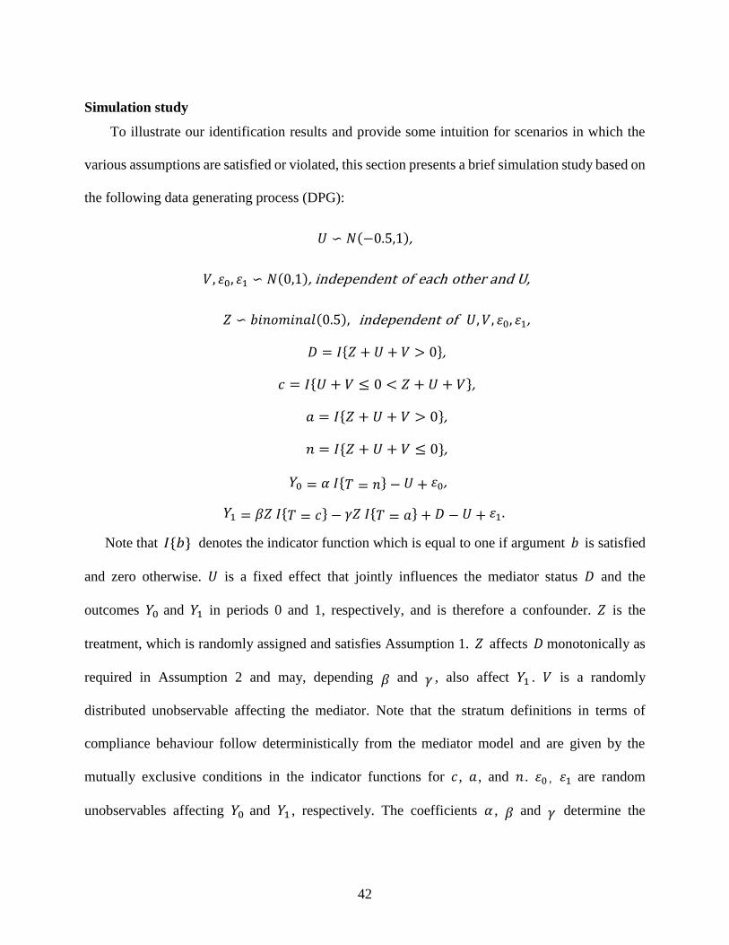
Simulation study
To illustrate our identification results and provide some intuition for scenarios in which the
various assumptions are satisfied or violated, this section presents a brief simulation study based on
the following data generating process (DPG):
𝑈 ∽ 𝑁(−0.5,1),
𝑉, 휀0, 휀1 ∽ 𝑁(0,1), independent of each other and U,
𝑍 ∽ 𝑏𝑖𝑛𝑜𝑚𝑖𝑛𝑎𝑙(0.5), independent of 𝑈, 𝑉, 휀0, 휀1,
𝐷 = 𝐼{𝑍 + 𝑈 + 𝑉 > 0},
𝑐 = 𝐼{𝑈 + 𝑉 ≤ 0 < 𝑍 + 𝑈 + 𝑉},
𝑎 = 𝐼{𝑍 + 𝑈 + 𝑉 > 0},
𝑛 = 𝐼{𝑍 + 𝑈 + 𝑉 ≤ 0},
𝑌0 = 𝛼 𝐼{𝑇 = 𝑛} − 𝑈 + 휀0,
𝑌1 = 𝛽𝑍 𝐼{𝑇 = 𝑐} − 𝛾𝑍 𝐼{𝑇 = 𝑎} + 𝐷 − 𝑈 + 휀1.
Note that 𝐼{𝑏} denotes the indicator function which is equal to one if argument 𝑏 is satisfied
and zero otherwise. 𝑈 is a fixed effect that jointly influences the mediator status 𝐷 and the
outcomes 𝑌0 and 𝑌1 in periods 0 and 1, respectively, and is therefore a confounder. 𝑍 is the
treatment, which is randomly assigned and satisfies Assumption 1. 𝑍 affects 𝐷 monotonically as
required in Assumption 2 and may, depending 𝛽 and 𝛾 , also affect 𝑌1 . 𝑉 is a randomly
distributed unobservable affecting the mediator. Note that the stratum definitions in terms of
compliance behaviour follow deterministically from the mediator model and are given by the
mutually exclusive conditions in the indicator functions for 𝑐 , 𝑎 , and 𝑛 . 휀0 , 휀1 are random
unobservables affecting 𝑌0 and 𝑌1 , respectively. The coefficients 𝛼 , 𝛽 and 𝛾 determine the
43
outcomes and/or effects for specific strata as well as which of our identifying assumptions are (not)
satisfied.
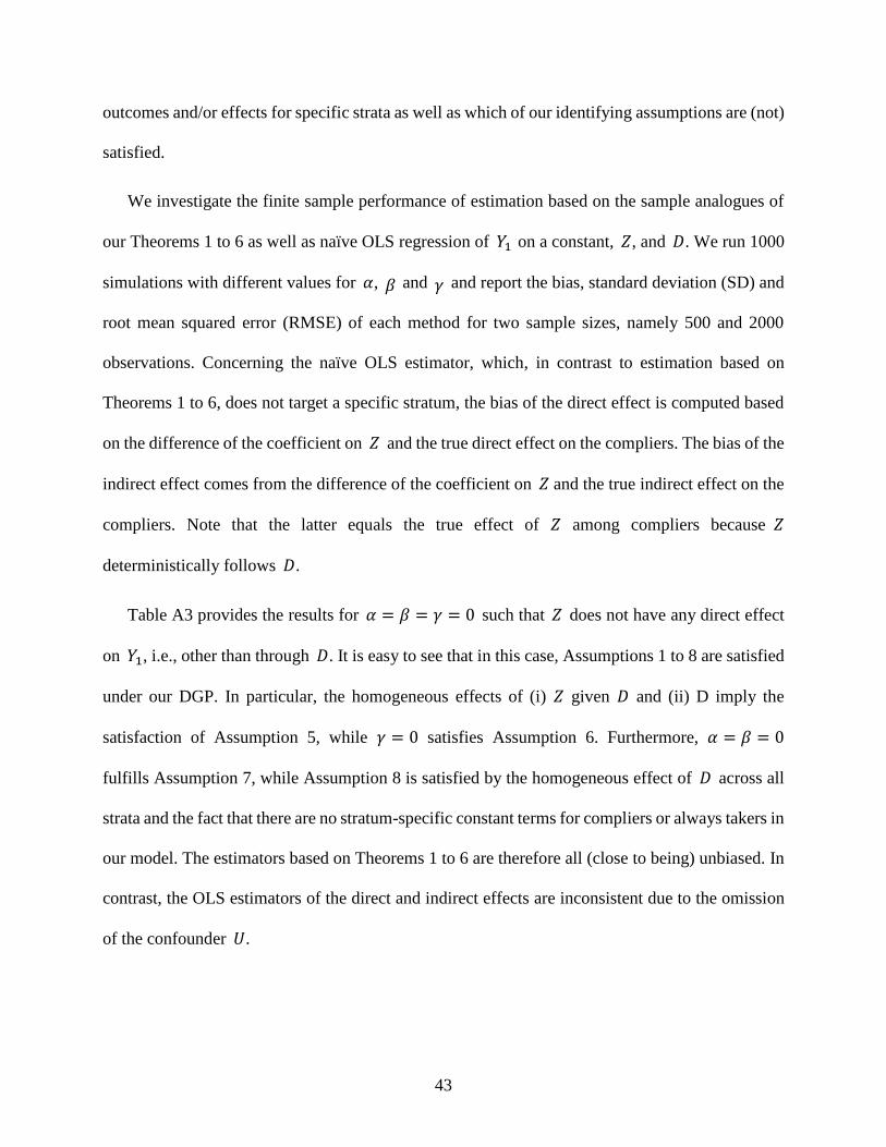
We investigate the finite sample performance of estimation based on the sample analogues of
our Theorems 1 to 6 as well as naïve OLS regression of 𝑌1 on a constant, 𝑍, and 𝐷. We run 1000
simulations with different values for 𝛼, 𝛽 and 𝛾 and report the bias, standard deviation (SD) and
root mean squared error (RMSE) of each method for two sample sizes, namely 500 and 2000
observations. Concerning the naïve OLS estimator, which, in contrast to estimation based on
Theorems 1 to 6, does not target a specific stratum, the bias of the direct effect is computed based
on the difference of the coefficient on 𝑍 and the true direct effect on the compliers. The bias of the
indirect effect comes from the difference of the coefficient on 𝑍 and the true indirect effect on the
compliers. Note that the latter equals the true effect of 𝑍 among compliers because 𝑍
deterministically follows 𝐷.
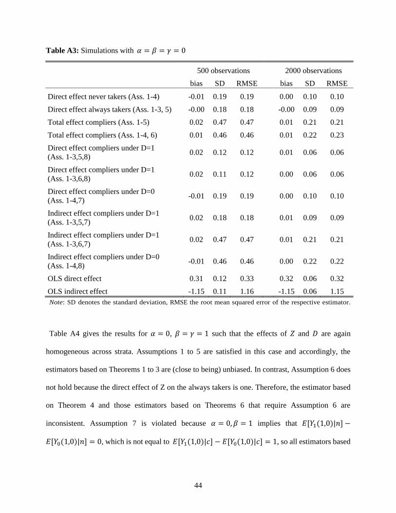
Table A3 provides the results for 𝛼 = 𝛽 = 𝛾 = 0 such that 𝑍 does not have any direct effect
on 𝑌1, i.e., other than through 𝐷. It is easy to see that in this case, Assumptions 1 to 8 are satisfied
under our DGP. In particular, the homogeneous effects of (i) 𝑍 given 𝐷 and (ii) D imply the
satisfaction of Assumption 5, while 𝛾 = 0 satisfies Assumption 6. Furthermore, 𝛼 = 𝛽 = 0
fulfills Assumption 7, while Assumption 8 is satisfied by the homogeneous effect of 𝐷 across all
strata and the fact that there are no stratum-specific constant terms for compliers or always takers in
our model. The estimators based on Theorems 1 to 6 are therefore all (close to being) unbiased. In
contrast, the OLS estimators of the direct and indirect effects are inconsistent due to the omission
of the confounder 𝑈.
44
Table A3: Simulations with 𝛼 = 𝛽 = 𝛾 = 0
500 observations
2000 observations
bias SD RMSE
bias SD RMSE
Direct effect never takers (Ass. 1-4) -0.01 0.19 0.19
0.00 0.10 0.10
Direct effect always takers (Ass. 1-3, 5) -0.00 0.18 0.18
-0.00 0.09 0.09
Total effect compliers (Ass. 1-5) 0.02 0.47 0.47
0.01 0.21 0.21
Total effect compliers (Ass. 1-4, 6) 0.01 0.46 0.46
0.01 0.22 0.23
Direct effect compliers under D=1
(Ass. 1-3,5,8) 0.02 0.12 0.12
0.01 0.06 0.06
Direct effect compliers under D=1
(Ass. 1-3,6,8) 0.02 0.11 0.12
0.00 0.06 0.06
Direct effect compliers under D=0
(Ass. 1-4,7) -0.01 0.19 0.19
0.00 0.10 0.10
Indirect effect compliers under D=1
(Ass. 1-3,5,7) 0.02 0.18 0.18
0.01 0.09 0.09
Indirect effect compliers under D=1
(Ass. 1-3,6,7) 0.02 0.47 0.47
0.01 0.21 0.21
Indirect effect compliers under D=0
(Ass. 1-4,8) -0.01 0.46 0.46
0.00 0.22 0.22
OLS direct effect 0.31 0.12 0.33
0.32 0.06 0.32
OLS indirect effect -1.15 0.11 1.16
-1.15 0.06 1.15
Note: SD denotes the standard deviation, RMSE the root mean squared error of the respective estimator.
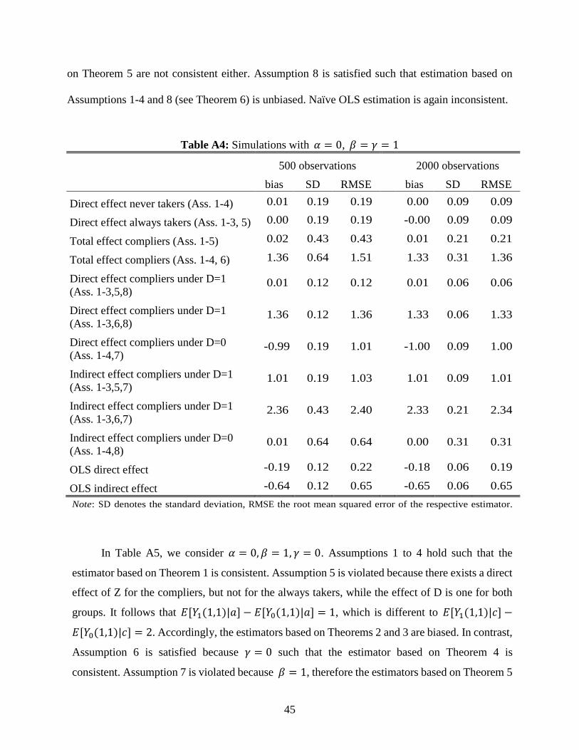
Table A4 gives the results for 𝛼 = 0, 𝛽 = 𝛾 = 1 such that the effects of 𝑍 and 𝐷 are again
homogeneous across strata. Assumptions 1 to 5 are satisfied in this case and accordingly, the
estimators based on Theorems 1 to 3 are (close to being) unbiased. In contrast, Assumption 6 does
not hold because the direct effect of Z on the always takers is one. Therefore, the estimator based
on Theorem 4 and those estimators based on Theorems 6 that require Assumption 6 are
inconsistent. Assumption 7 is violated because 𝛼 = 0, 𝛽 = 1 implies that 𝐸[𝑌1(1,0)|𝑛] −
𝐸[𝑌0(1,0)|𝑛] = 0, which is not equal to 𝐸[𝑌1(1,0)|𝑐] − 𝐸[𝑌0(1,0)|𝑐] = 1, so all estimators based
45
on Theorem 5 are not consistent either. Assumption 8 is satisfied such that estimation based on
Assumptions 1-4 and 8 (see Theorem 6) is unbiased. Naïve OLS estimation is again inconsistent.
Table A4: Simulations with 𝛼 = 0, 𝛽 = 𝛾 = 1
500 observations
2000 observations
bias SD RMSE
bias SD RMSE
Direct effect never takers (Ass. 1-4) 0.01 0.19 0.19 0.00 0.09 0.09
Direct effect always takers (Ass. 1-3, 5) 0.00 0.19 0.19 -0.00 0.09 0.09
Total effect compliers (Ass. 1-5) 0.02 0.43 0.43 0.01 0.21 0.21
Total effect compliers (Ass. 1-4, 6) 1.36 0.64 1.51 1.33 0.31 1.36
Direct effect compliers under D=1
(Ass. 1-3,5,8) 0.01 0.12 0.12 0.01 0.06 0.06
Direct effect compliers under D=1
(Ass. 1-3,6,8) 1.36 0.12 1.36 1.33 0.06 1.33
Direct effect compliers under D=0
(Ass. 1-4,7) -0.99 0.19 1.01 -1.00 0.09 1.00
Indirect effect compliers under D=1
(Ass. 1-3,5,7) 1.01 0.19 1.03 1.01 0.09 1.01
Indirect effect compliers under D=1
(Ass. 1-3,6,7) 2.36 0.43 2.40 2.33 0.21 2.34
Indirect effect compliers under D=0
(Ass. 1-4,8) 0.01 0.64 0.64 0.00 0.31 0.31
OLS direct effect -0.19 0.12 0.22 -0.18 0.06 0.19
OLS indirect effect -0.64 0.12 0.65 -0.65 0.06 0.65
Note: SD denotes the standard deviation, RMSE the root mean squared error of the respective estimator.
In Table A5, we consider 𝛼 = 0, 𝛽 = 1, 𝛾 = 0. Assumptions 1 to 4 hold such that the
estimator based on Theorem 1 is consistent. Assumption 5 is violated because there exists a direct
effect of Z for the compliers, but not for the always takers, while the effect of D is one for both
groups. It follows that 𝐸[𝑌1(1,1)|𝑎] − 𝐸[𝑌0(1,1)|𝑎] = 1, which is different to 𝐸[𝑌1(1,1)|𝑐] −
𝐸[𝑌0(1,1)|𝑐] = 2. Accordingly, the estimators based on Theorems 2 and 3 are biased. In contrast,
Assumption 6 is satisfied because 𝛾 = 0 such that the estimator based on Theorem 4 is
consistent. Assumption 7 is violated because 𝛽 = 1, therefore the estimators based on Theorem 5
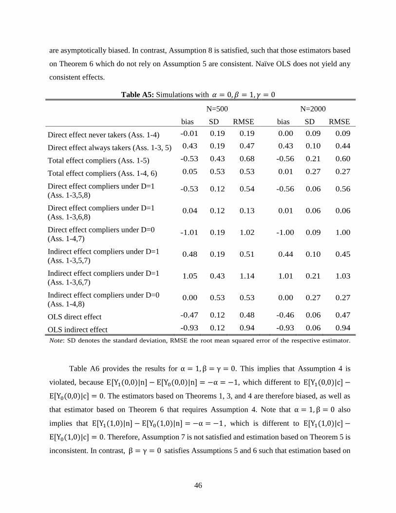
46
are asymptotically biased. In contrast, Assumption 8 is satisfied, such that those estimators based
on Theorem 6 which do not rely on Assumption 5 are consistent. Naïve OLS does not yield any
consistent effects.
Table A5: Simulations with 𝛼 = 0, 𝛽 = 1, 𝛾 = 0
N=500
N=2000
bias SD RMSE
bias SD RMSE
Direct effect never takers (Ass. 1-4) -0.01 0.19 0.19 0.00 0.09 0.09
Direct effect always takers (Ass. 1-3, 5) 0.43 0.19 0.47 0.43 0.10 0.44
Total effect compliers (Ass. 1-5) -0.53 0.43 0.68 -0.56 0.21 0.60
Total effect compliers (Ass. 1-4, 6) 0.05 0.53 0.53 0.01 0.27 0.27
Direct effect compliers under D=1
(Ass. 1-3,5,8) -0.53 0.12 0.54 -0.56 0.06 0.56
Direct effect compliers under D=1
(Ass. 1-3,6,8) 0.04 0.12 0.13 0.01 0.06 0.06
Direct effect compliers under D=0
(Ass. 1-4,7) -1.01 0.19 1.02 -1.00 0.09 1.00
Indirect effect compliers under D=1
(Ass. 1-3,5,7) 0.48 0.19 0.51 0.44 0.10 0.45
Indirect effect compliers under D=1
(Ass. 1-3,6,7) 1.05 0.43 1.14 1.01 0.21 1.03
Indirect effect compliers under D=0
(Ass. 1-4,8) 0.00 0.53 0.53 0.00 0.27 0.27
OLS direct effect -0.47 0.12 0.48 -0.46 0.06 0.47
OLS indirect effect -0.93 0.12 0.94 -0.93 0.06 0.94
Note: SD denotes the standard deviation, RMSE the root mean squared error of the respective estimator.
Table A6 provides the results for α = 1, β = γ = 0. This implies that Assumption 4 is
violated, because E[Y1(0,0)|n] − E[Y0(0,0)|n] = −α = −1, which different to E[Y1(0,0)|c] −
E[Y0(0,0)|c] = 0. The estimators based on Theorems 1, 3, and 4 are therefore biased, as well as
that estimator based on Theorem 6 that requires Assumption 4. Note that α = 1, β = 0 also
implies that E[Y1(1,0)|n] − E[Y0(1,0)|n] = −α = −1 , which is different to E[Y1(1,0)|c] −
E[Y0(1,0)|c] = 0. Therefore, Assumption 7 is not satisfied and estimation based on Theorem 5 is
inconsistent. In contrast, β = γ = 0 satisfies Assumptions 5 and 6 such that estimation based on
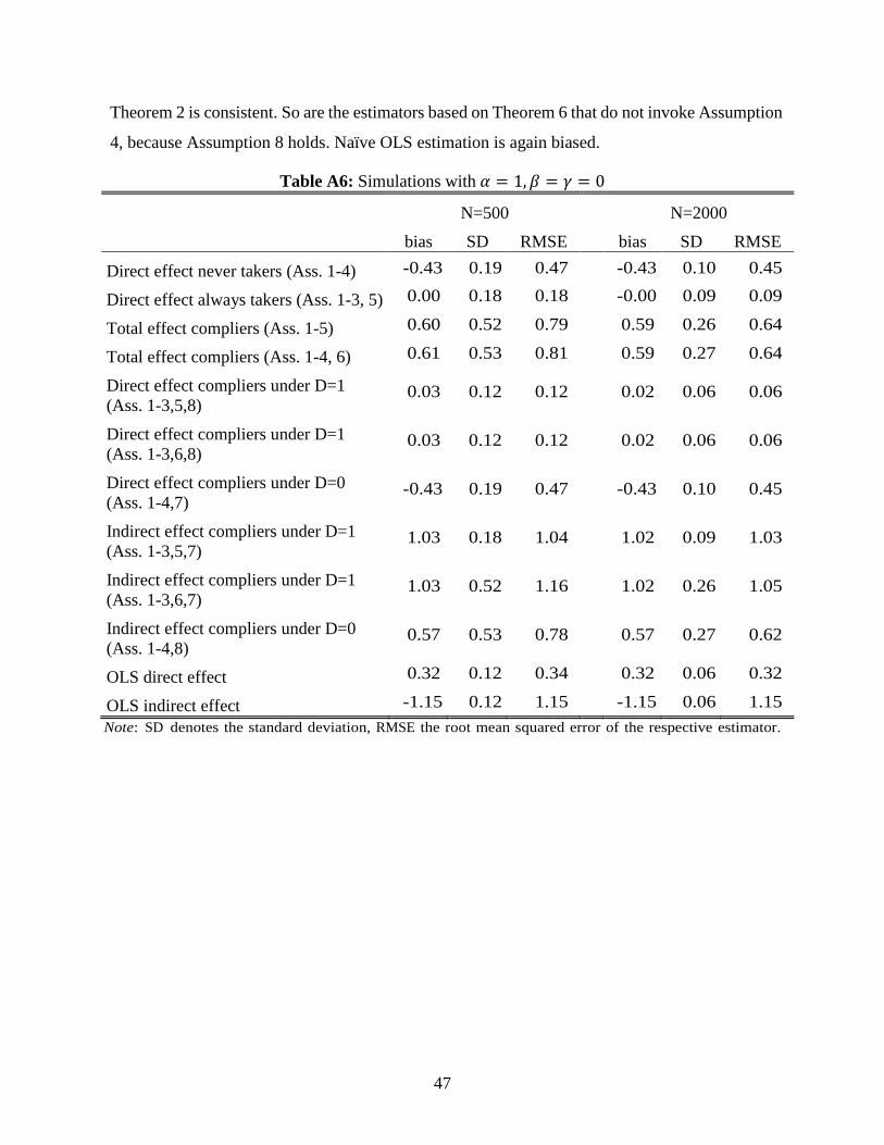
47
Theorem 2 is consistent. So are the estimators based on Theorem 6 that do not invoke Assumption
4, because Assumption 8 holds. Naïve OLS estimation is again biased.
Table A6: Simulations with 𝛼 = 1, 𝛽 = 𝛾 = 0
N=500
N=2000
bias SD RMSE
bias SD RMSE
Direct effect never takers (Ass. 1-4) -0.43 0.19 0.47 -0.43 0.10 0.45
Direct effect always takers (Ass. 1-3, 5) 0.00 0.18 0.18 -0.00 0.09 0.09
Total effect compliers (Ass. 1-5) 0.60 0.52 0.79 0.59 0.26 0.64
Total effect compliers (Ass. 1-4, 6) 0.61 0.53 0.81 0.59 0.27 0.64
Direct effect compliers under D=1
(Ass. 1-3,5,8) 0.03 0.12 0.12 0.02 0.06 0.06
Direct effect compliers under D=1
(Ass. 1-3,6,8) 0.03 0.12 0.12 0.02 0.06 0.06
Direct effect compliers under D=0
(Ass. 1-4,7) -0.43 0.19 0.47 -0.43 0.10 0.45
Indirect effect compliers under D=1
(Ass. 1-3,5,7) 1.03 0.18 1.04 1.02 0.09 1.03
Indirect effect compliers under D=1
(Ass. 1-3,6,7) 1.03 0.52 1.16 1.02 0.26 1.05
Indirect effect compliers under D=0
(Ass. 1-4,8) 0.57 0.53 0.78 0.57 0.27 0.62
OLS direct effect 0.32 0.12 0.34 0.32 0.06 0.32
OLS indirect effect -1.15 0.12 1.15 -1.15 0.06 1.15
Note: SD denotes the standard deviation, RMSE the root mean squared error of the respective estimator.
48
Literature
Angrist, J. (1990). Lifetime Earnings and the Vietnam Era Draft Lottery: Evidence from Social
Security Administrative Records. American Economic Review, 80(3), pp. 313-336.
Angrist, J. (1991). The Draft Lottery and Voluntary Enlistment in the Vietnam Era. Journal of the
American Statistical Association.
Angrist, J. D., Chen, S. H., & Frandsen, B. R. (2010). Did Vietnam veterans get sicker in the
1990s? The complicated effects of military service on self-reported health. Journal of
Public Economics, 94(11-12), pp. 824-837.
Angrist, J. D., Imbens, G. W., & Rubin, D. B. (1996). Identification of Causal Effects Using
Instrumental Variables. Journal of the American Statistical Association, 91(434), pp.
444-455.
Bachman, J. G. (1999). Young Men in High School and Beyond: A Summary of Findings from the
Youth in Transition Project, 1966-1974. Ann Arbor, MI: Inter-university Consortium for
Political and Social Research.
Baskir, L. M., & Strauss, W. A. (1978). Chance and Circumstance: The Draft, The War, and the
Vietnam Generation. New York: Alfred A Knopf.
Bergan, D. (2009). The Draft Lottery and Attitudes Towards the Vietnam War. Public Opinion
Quarterly, 73(2), pp. 379-384.
Card, D., & Lemieux, T. (2001). Going to College to Avoid the Draft: The Unintended Legacy of
the Vietnam War. American Economic Review, 91(2), pp. 97-102.
Dee, T. (2004). Are there civic returns to education? Journal of Public Economics, 88, pp.
1697-1720.
Deuchert, E., & Huber, M. (2014). A cautionary tale about control variables in IV estimation.
University of St. Gallen, School of Economics and Political Science: Economics Working
Paper Series 1439.
Erikson, R., & Stoker, L. (2011). Caught in the draft: The effects of Vietnam draft lottery status on
political attitudes. American Political Science Review, 105(2), pp. 221-237.
Fienberg, S. (1971). Randomization and Social Affairs: The 1970 Draft Lottery. Science,
171(3968), pp. 255-261.
49
Flores, C., & Flores-Lagunes, A. (2009). Identification and Estimation of Causal Mechanisms and
Net Effects of a Treatment under UnconfoundednessFlores-Lagunes. IZA Discussion Paper
No. 4237.
Frangakis, C., & Rubin, D. (2002). Principal stratification in causal inference. Biometrics, 58(1),
pp. 21-29.
Frölich, M., & Huber, M. (2014). Direct and Indirect Treatment Effects: Causal Chains and
Mediation Analysis with Instrumental Variables. IZA DP No. 8280.
Gimbel, C., & Booth, A. (1996). Who Fought in Vietnam? Social Forces, 74(4), pp. 1137-1157.
Hagan, J. (2001). Northern passage : American Vietnam War resisters in Canada. Camebridge:
Harvard University Press.
Hong, G. (2010). Ratio of mediator probability weighting for estimating natural direct and indirect
effects. Proceedings of the American Statistical Association, Biometrics Section, p.
24012415.
Huber, M. (2014). Identifying causal mechanisms (primarily) based on inverse probability
weighting. Journal of Applied Econometrics, 29, pp. 920-943.
Imai, K., Keele, L., & Yamamoto, T. (2010). Identification, Inference and Sensitivity Analysis for
Causal Mediation Effects. Statistical Science, 25(1), pp. 1-144.
Imai, K., Tingley, D., & Yamamoto, T. (2013). Experimental Designs for Identifying Causal
Mechanisms. Journal of the Royal Statistical Society, Series A (Statistics in Society),
173(1), pp. 5-51.
Imbens, G. W., & Angrist, J. D. (1994). Identification and Estimation of Local Average Treatment
Effects. Econometrica, 62(2), pp. 467-475.
Jones, J. (2005). Contending statistics : the numbers for U.S. Vietnam War resisters in Canada.
Vancouver: Quarter Sheaf.
Kam, C. D., & Palmer, C. L. (2008). Reconsidering the Effects of Education on Political
Participation. Journal of Politics, 70(3), pp. 612-631.
Kuziemko, I. (2010). Did the Vietnam Draft Increase Human Capital Dispersion?
Draft-Avoidance Behavior by Race and Class. Princeton and NBER: working paper.
50
Lechner, M. (2011). The Estimation of Causal Effects by Difference-in-Difference Methods.
Foundations and Trends® in Econometrics, 4(3), pp. 165-224.
Marshall, J. (2014). Learning to be conservative: How staying in high school changes political
preferences in the United States and Great Britain. working paper.
Milligan, K., Moretti, E., & Oreopoulos, P. (n.d.). Does education improve citizenship? Evidence
from the United States and the United Kingdom. Journal of Public Economics2004, 88, pp.
174-189.
Milstein Sondheimer, R., & Green, D. (2009). Using Experiments to Estimate the Effects of
Education on Voter Turnout. American Journal of Political Science, 54(1), pp. 174-189.
Morten, R., Tyran, J., & Wenström, E. (2011). Income and Ideology: How Personality Traits,
Cognitive Abilities, and Education Shape Political Attitudes. working paper.
Pearl, J. (2001). Direct and Indirect Effects. Proceedings of the Seventeenth Conference on
Uncertainty in Artificial Intelligence, pp. 411-420.
Petersen, M., Sinisi, S., & van der Laan, M. (2006). Estimation of direct causal effects.
Epidemiology, 17, pp. 276–284.
Robins, J. M. (2003). Semantics of causal DAG models and the identification. In P. J. Green, N. L.
Hjort, & S. Richardson, Highly structured stochastic systems (pp. 70–81). New York:
Oxford University Press.
Robins, J., & Greenland, S. (1992). Identifiability and exchangeability for direct and indirect
effects. Epidemiology, 3(2), pp. 143-155.
Rubin, D. B. (1974). Estimating causal effects of treatments in randomized and nonrandomized
studies. Journal of Educational Psychology, 66(5), pp. 688-701.
Rubin, D. B. (2004). Direct and indirect causal effects via potential outcomes. Scandinavian
Journal of Statistics, 31, pp. 161–170.
Tchetgen Tchetgen, E., & Shpitser, I. (2012). Semiparametric theory for causal mediation analysis:
Efficiency bounds, multiple robustness and sensitivity analysis. Annals of Statistics, 40(3),
pp. 1816-1845.
51
VanderWeele, T. (2009). Marginal structural models for the estimation of direct and indirect
effects. Epidemiology, 20, pp. 18–2.
VanderWeele, T. J. (2008). Simple relations between principal stratification and direct and indirect
effects. Statistics and Probability Letters, 78, pp. 2957–2962.
VanderWeele, T. J. (2012). Comments: Should Principal Stratification Be Used to Study
Mediational Processes? Journal of Research on Educational Effectiveness(5), pp. 245–249.
Yamamoto, T. (2013). Identification and Estimation of Causal Mediation Effects with Treatment
Noncompliance. working paper.
Zheng, W., & van der Laan, J. (2012). Targeted maximum likelihood estimation of natural direct
effects. International Journal of Biostatistics, 8, p. Article 1.
Recommended