Differential equations with time delay
Marek Bodnar
Faculty of Mathematics, Informatics and Mechanics,Institute of Applied Mathematics and Mechanics,
University of Warsaw
MIM ColloquiumDecember 8th, 2016
Gallery of properties Stability Models Linear equation Non-negativity Phase space Continuation Step method
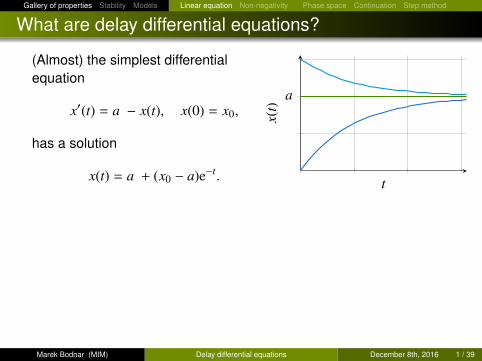
What are delay differential equations?
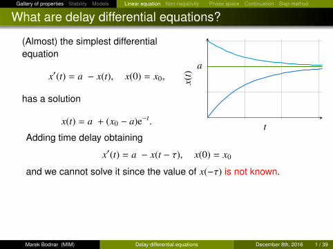
(Almost) the simplest differentialequation
x′(t) = a − x(t), x(0) = x0,
has a solution
x(t) = a + (x0 − a)e−t.
a
t
x(t)
Adding time delay obtaining
x′(t) = a − x(t − τ), x(0) = x0
and we cannot solve it since the value of x(−τ) is not known.In general, there are no solutions of this linear equation that can beexpressed in terms of elementary functions.
Corollary
A proper phase space is a space of functions.
Marek Bodnar (MIM) Delay differential equations December 8th, 2016 1 / 39
Gallery of properties Stability Models Linear equation Non-negativity Phase space Continuation Step method
What are delay differential equations?
(Almost) the simplest differentialequation
x′(t) = a − x(t), x(0) = x0,
has a solution
x(t) = a + (x0 − a)e−t.
a
t
x(t)
Adding time delay obtaining
x′(t) = a − x(t − τ), x(0) = x0
and we cannot solve it since the value of x(−τ) is not known.
In general, there are no solutions of this linear equation that can beexpressed in terms of elementary functions.
Corollary
A proper phase space is a space of functions.
Marek Bodnar (MIM) Delay differential equations December 8th, 2016 1 / 39
Gallery of properties Stability Models Linear equation Non-negativity Phase space Continuation Step method
What are delay differential equations?
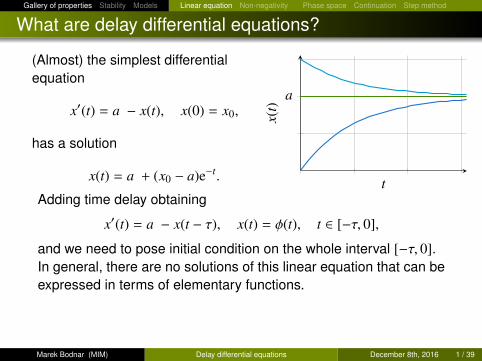
(Almost) the simplest differentialequation
x′(t) = a − x(t), x(0) = x0,
has a solution
x(t) = a + (x0 − a)e−t.
a
t
x(t)
Adding time delay obtaining
x′(t) = a − x(t − τ), x(t) = φ(t), t ∈ [−τ, 0],
and we need to pose initial condition on the whole interval [−τ, 0].In general, there are no solutions of this linear equation that can beexpressed in terms of elementary functions.
Corollary
A proper phase space is a space of functions.
Marek Bodnar (MIM) Delay differential equations December 8th, 2016 1 / 39
Gallery of properties Stability Models Linear equation Non-negativity Phase space Continuation Step method
What are delay differential equations?
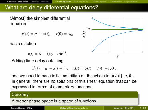
(Almost) the simplest differentialequation
x′(t) = a − x(t), x(0) = x0,
has a solution
x(t) = a + (x0 − a)e−t.
a
t
x(t)
Adding time delay obtaining
x′(t) = a − x(t − τ), x(t) = φ(t), t ∈ [−τ, 0],
and we need to pose initial condition on the whole interval [−τ, 0].In general, there are no solutions of this linear equation that can beexpressed in terms of elementary functions.
Corollary
A proper phase space is a space of functions.Marek Bodnar (MIM) Delay differential equations December 8th, 2016 1 / 39
Gallery of properties Stability Models Linear equation Non-negativity Phase space Continuation Step method
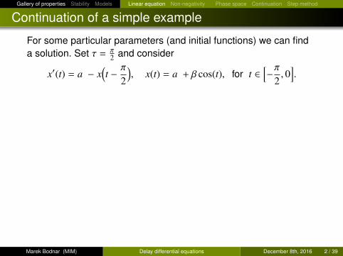
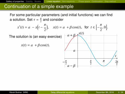
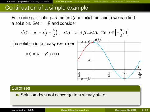
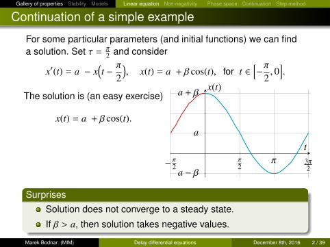
Continuation of a simple example
For some particular parameters (and initial functions) we can finda solution. Set τ = π
2 and consider
x′(t) = a − x(t − π
2
), x(t) = a + β cos(t), for t ∈
[−π
2, 0
].
The solution is (an easy exercise)
x(t) = a + β cos(t).
Surprises
Solution does not converge to a steady state.
If β > a, then solution takes negative values.
−π2 π2
π 3π2a − β
a
a + β
t
x(t)
Marek Bodnar (MIM) Delay differential equations December 8th, 2016 2 / 39
Gallery of properties Stability Models Linear equation Non-negativity Phase space Continuation Step method
Continuation of a simple example
For some particular parameters (and initial functions) we can finda solution. Set τ = π
2 and consider
x′(t) = a − x(t − π
2
), x(t) = a + β cos(t), for t ∈
[−π
2, 0
].
The solution is (an easy exercise)
x(t) = a + β cos(t).
SurprisesSolution does not converge to a steady state.
If β > a, then solution takes negative values.
−π2 π2
π 3π2a − β
a
a + β
t
x(t)
Marek Bodnar (MIM) Delay differential equations December 8th, 2016 2 / 39
Gallery of properties Stability Models Linear equation Non-negativity Phase space Continuation Step method
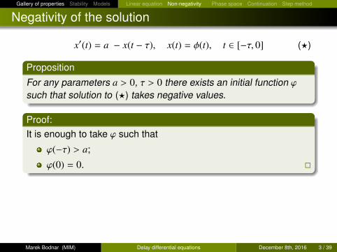
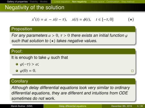
Negativity of the solution
x′(t) = a − x(t − τ), x(t) = φ(t), t ∈ [−τ, 0] (?)
Proposition
For any parameters a > 0, τ > 0 there exists an initial function ϕsuch that solution to (?) takes negative values.
Proof:It is enough to take ϕ such that
ϕ(−τ) > a;
ϕ(0) = 0. �
Corollary
Although delay differential equations look very similar to ordinarydifferential equations, they are different and intuitions from ODEsometimes do not work.
Marek Bodnar (MIM) Delay differential equations December 8th, 2016 3 / 39
Gallery of properties Stability Models Linear equation Non-negativity Phase space Continuation Step method
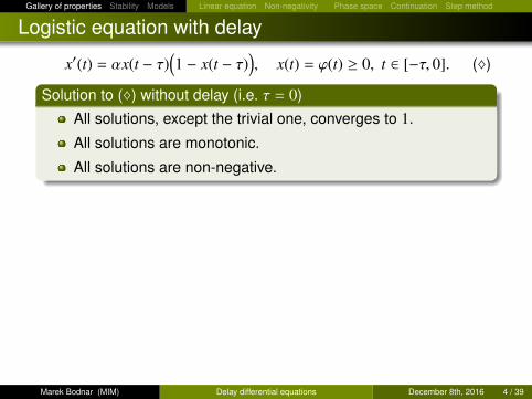
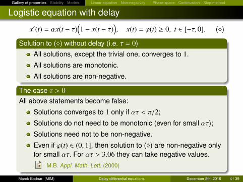
Logistic equation with delay
x′(t) = αx(t − τ)(1 − x(t − τ)
), x(t) = ϕ(t) ≥ 0, t ∈ [−τ, 0]. (♦)
Solution to (♦) without delay (i.e. τ = 0)
All solutions, except the trivial one, converges to 1.
All solutions are monotonic.
All solutions are non-negative.
The case τ > 0All above statements become false:
Solutions converges to 1 only if ατ < π/2;
Solutions do not need to be monotonic (even for small ατ);
Solutions need not to be non-negative.
Even if ϕ(t) ∈ (0, 1], then solution to (♦) are non-negative onlyfor small ατ. For ατ > 3.06 they can take negative values.
M.B. Appl. Math. Lett. (2000)
Marek Bodnar (MIM) Delay differential equations December 8th, 2016 4 / 39
Gallery of properties Stability Models Linear equation Non-negativity Phase space Continuation Step method
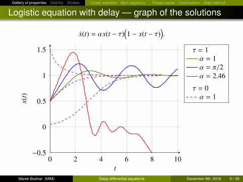
Logistic equation with delay — graph of the solutions
x(t) = αx(t − τ)(1 − x(t − τ)
).
0 2 4 6 8 10−0.5
0
0.5
1
1.5
t
x(t)
τ = 1α = 1α = π/2α = 2.46
τ = 0α = 1
Marek Bodnar (MIM) Delay differential equations December 8th, 2016 5 / 39
Gallery of properties Stability Models Linear equation Non-negativity Phase space Continuation Step method
Hutchinson model and open problem
Hutchinson model
x′(t) = αx(t)(1 − x(t − τ)
)For ατ < 37/24 all solutions converges to x = 1, except thetrivial one.
At ατ = π/2 the Hopf bifurcation occurs (the steady statebecomes unstable and periodic solution arises).
For ατ < π/2 the steady state is locally stable.
Wright’s hypothesis:
The steady state is globally stable for all ατ < π/2.
It is not known if the hyphothesis is true for 37/24 < ατ < π/2.
I say few words more about logistic equation later.
Marek Bodnar (MIM) Delay differential equations December 8th, 2016 6 / 39
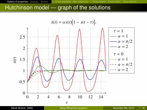
Gallery of properties Stability Models Linear equation Non-negativity Phase space Continuation Step method
Hutchinson model — graph of the solutions
x(t) = αx(t)(1 − x(t − τ)
).
0 2 4 6 8 10 12 140
0.5
1
1.5
2
2.5
t
x(t)
τ = 1α = 1α = π/2α = 2
τ = 0α = 1α = π/2α = 2
Marek Bodnar (MIM) Delay differential equations December 8th, 2016 7 / 39
Gallery of properties Stability Models Linear equation Non-negativity Phase space Continuation Step method
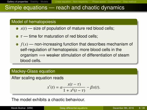
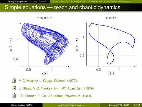
Simple equations — reach and chaotic dynamics
Model of hematopoiesis
x(t) — size of population of mature red blood cells;
τ — time for maturation of red blood cells;
f (x) — non-increasing function that describes mechanism ofself-regulation of hematopeisis: more blood cells in theorganism =⇒ weaker stimulation of differentiation of steamblood cells.
Mackey-Glass equation
After scaling equation reads
x′(t) = αx(t − τ)
1 + xk(t − τ)− βx(t).
The model exhibits a chaotic behaviour.
Marek Bodnar (MIM) Delay differential equations December 8th, 2016 8 / 39
Gallery of properties Stability Models Linear equation Non-negativity Phase space Continuation Step method
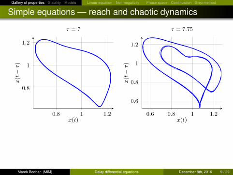
Simple equations — reach and chaotic dynamics
0.8 1 1.2
0.8
1
1.2
x(t)
x(t−τ)
τ = 7
0.6 0.8 1 1.2
0.6
0.8
1
1.2
x(t)x(t−
τ)
τ = 7.75
M.C. Mackey, L. Glass, Science, (1977).
L. Glass, M.C. Mackey, Ann. NY. Acad. Sci., (1979).
J.D. Farmer, E. Ott, J.A. Yorke, Physica D, (1983).
Marek Bodnar (MIM) Delay differential equations December 8th, 2016 9 / 39
Gallery of properties Stability Models Linear equation Non-negativity Phase space Continuation Step method
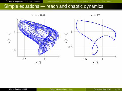
Simple equations — reach and chaotic dynamics
0.5 1
0.5
1
x(t)
x(t−
τ)
τ = 9.696
0.5 1
0.5
1
x(t)x(t−τ)
τ = 12
M.C. Mackey, L. Glass, Science, (1977).
L. Glass, M.C. Mackey, Ann. NY. Acad. Sci., (1979).
J.D. Farmer, E. Ott, J.A. Yorke, Physica D, (1983).
Marek Bodnar (MIM) Delay differential equations December 8th, 2016 9 / 39
Gallery of properties Stability Models Linear equation Non-negativity Phase space Continuation Step method
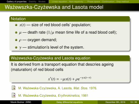
Wazewszka-Czyzewska and Lasota model
Notationx(t) — size of red blood cells’ population;
µ — death rate (1/µ mean time life of a read blood cell);
ρ — oxygen demand;
γ — stimulation’s level of the system.
Wazewszka-Czyzewska and Lasota equation
It is derived from a transport equation that descries ageing(maturation) of red blood cells
x′(t) = −µx(t) + ρe−γx(t−τ)
M. Wazewska-Czyzewska, A. Lasota, Mat. Stos. 1976.
M. Wazewska-Czyzewska, Erythrokinetics, 1981
Marek Bodnar (MIM) Delay differential equations December 8th, 2016 10 / 39
Gallery of properties Stability Models Linear equation Non-negativity Phase space Continuation Step method
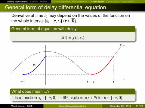
General form of delay differential equationDerivative at time t0 may depend on the values of the function onthe whole interval [t0 − τ, t0] (τ ∈ �).
General form of equation with delay
x(t) = f (t, xt)
x
tt − τ−τ
xt
What does mean xt?It is a function xt : [−τ, 0]→ �n, xt(θ) = x(t + θ) for θ ∈ [−τ, 0].
Marek Bodnar (MIM) Delay differential equations December 8th, 2016 11 / 39
Gallery of properties Stability Models Linear equation Non-negativity Phase space Continuation Step method
Phase space
For finite delay (τ < ∞)
Usually we consider the space
C = C([−τ, 0];�n) ,
of continuous functions defined on [−τ, 0].
There exist a few papers at which the space Lp is considered.
Regularity of solutions
Assume that f ∈ Ck, then for 1 ≤ ` ≤ k + 1
xt ∈ C`, for t ≥ t0 + `τ.
Marek Bodnar (MIM) Delay differential equations December 8th, 2016 12 / 39
Gallery of properties Stability Models Linear equation Non-negativity Phase space Continuation Step method
Continuation of solutions
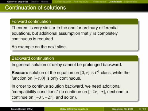
Forward continuationTheorem is very similar to the one for ordinary differentialequations, but additional assumption that f is completelycontinuous is required.
An example on the next slide.
Backward continuationIn general solution of delay cannot be prolonged backward.
Reason: solution of the equation on [0, τ] is C1 class, while thefunction on [−τ, 0] is only continuous.
In order to continue solution backward, we need additional“compatibility conditions” (to continue on [−2τ,−τ], next one tocontinue on [−3τ,−2τ], and so on).
Marek Bodnar (MIM) Delay differential equations December 8th, 2016 13 / 39
Gallery of properties Stability Models Linear equation Non-negativity Phase space Continuation Step method
Continuation of solutions
Forward continuationTheorem is very similar to the one for ordinary differentialequations, but additional assumption that f is completelycontinuous is required.
An example on the next slide.
Backward continuationIn general solution of delay cannot be prolonged backward.
Reason: solution of the equation on [0, τ] is C1 class, while thefunction on [−τ, 0] is only continuous.
In order to continue solution backward, we need additional“compatibility conditions” (to continue on [−2τ,−τ], next one tocontinue on [−3τ,−2τ], and so on).
Marek Bodnar (MIM) Delay differential equations December 8th, 2016 13 / 39
Gallery of properties Stability Models Linear equation Non-negativity Phase space Continuation Step method
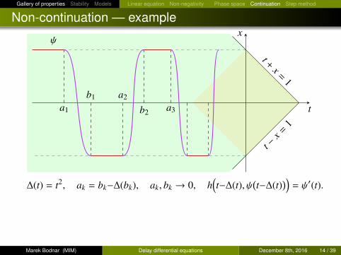
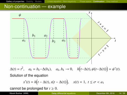
Non-continuation — example
t +x=
1
t −x =
1
t
x
a1
b1 a2
b2 a3
ψ
∆(t) = t2, ak = bk−∆(bk), ak, bk → 0, h(t−∆(t), ψ
(t−∆(t)
))= ψ′(t).
Solution of the equation
x′(t) = h(t − ∆(t), x
(t − ∆(t)
)), x(t) = 1, t ≤ σ < a1
cannot be prolonged for t ≥ 0.
Marek Bodnar (MIM) Delay differential equations December 8th, 2016 14 / 39
Gallery of properties Stability Models Linear equation Non-negativity Phase space Continuation Step method
Non-continuation — example
t +x=
1
t −x =
1
t
x
a1
b1 a2
b2 a3
ψ
∆(t) = t2, ak = bk−∆(bk), ak, bk → 0, h(t−∆(t), ψ
(t−∆(t)
))= ψ′(t).
Solution of the equation
x′(t) = h(t − ∆(t), x
(t − ∆(t)
)), x(t) = 1, t ≤ σ < a1
cannot be prolonged for t ≥ 0.Marek Bodnar (MIM) Delay differential equations December 8th, 2016 14 / 39
Gallery of properties Stability Models Linear equation Non-negativity Phase space Continuation Step method
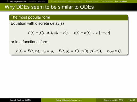
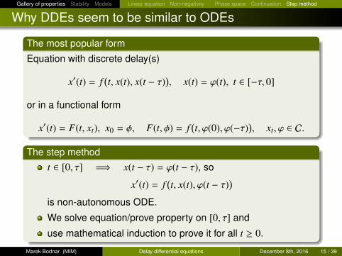
Why DDEs seem to be similar to ODEs
The most popular form
Equation with discrete delay(s)
x′(t) = f(t, x(t), x(t − τ)
), x(t) = ϕ(t), t ∈ [−τ, 0]
or in a functional form
x′(t) = F(t, xt), x0 = φ, F(t, φ) = f(t, ϕ(0), ϕ(−τ)
), xt, ϕ ∈ C.
The step methodt ∈ [0, τ] =⇒ x(t − τ) = ϕ(t − τ), so
x′(t) = f(t, x(t), ϕ(t − τ)
)is non-autonomous ODE.
We solve equation/prove property on [0, τ] and
use mathematical induction to prove it for all t ≥ 0.
Marek Bodnar (MIM) Delay differential equations December 8th, 2016 15 / 39
Gallery of properties Stability Models Linear equation Non-negativity Phase space Continuation Step method
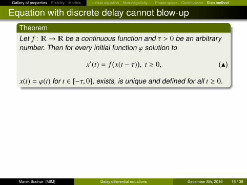
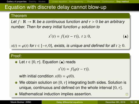
Equation with discrete delay cannot blow-up
TheoremLet f : �→ � be a continuous function and τ > 0 be an arbitrarynumber. Then for every initial function ϕ solution to
x′(t) = f(x(t − τ)
), t ≥ 0, (N)
x(t) = ϕ(t) for t ∈ [−τ, 0], exists, is unique and defined for all t ≥ 0.
Proof:Let t ∈ [0, τ]. Equation (N) reads
x′(t) = f(ϕ(t − τ)
).
with initial condition x(0) = ϕ(0).
We obtain solution on [0, τ] integrating both sides. Solution isunique, continuous and defined on the whole interval [0, τ].
Mathematical induction implies assertion. �
Marek Bodnar (MIM) Delay differential equations December 8th, 2016 16 / 39
Gallery of properties Stability Models Linear equation Non-negativity Phase space Continuation Step method
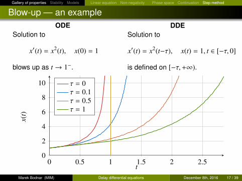
Blow-up — an exampleODE
Solution to
x′(t) = x2(t), x(0) = 1
blows up as t → 1−.
DDESolution to
x′(t) = x2(t−τ), x(t) = 1, t ∈ [−τ, 0]
is defined on [−τ,+∞).
0 0.5 1 1.5 2 2.50
2
4
6
8
10
t
x(t)
τ = 0τ = 0.1τ = 0.5τ = 1
Marek Bodnar (MIM) Delay differential equations December 8th, 2016 17 / 39
Gallery of properties Stability Models General theory One equation Two equations More equations or more delays
Stability of the steady state
Techniques1 Liapunov functional theorem, an analogous to the version for
ODEs. However, here V : C → �;
2 Linearization method (the most popular — I will discuss more);
3 Comparison with an appropriate discrete dynamical system(that is studying the behaviour for delay −→ +∞),
E. Liz, A. Ruiz-Herrera, J. Diff. Eqs., (2013).
M.B., J. Diff. Eqs, (2015)
Marek Bodnar (MIM) Delay differential equations December 8th, 2016 18 / 39
Gallery of properties Stability Models General theory One equation Two equations More equations or more delays
Liapunov functional — an example
Finding Liapunov functional
is as easy (or as difficult) as for ODEs. If we know Liapunovfunction for ODE version of the system we may try to add someintegral term.
Considerx′(t) = −a(t)x3(t) + b(t)x3(t − τ). (♣)
Assumptions:a, b : �→ � continuous and bounded;
a(t) ≥ δ, |b(t)| < qδ, for 0 < q < 1.
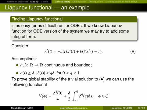
To prove global stability of the trivial solution to (♣) we can use thefollowing functional
V(φ) =φ4(0)
4+δ
2
∫ 0
−τφ6(s)ds, φ ∈ C
Marek Bodnar (MIM) Delay differential equations December 8th, 2016 19 / 39
Gallery of properties Stability Models General theory One equation Two equations More equations or more delays
Liapunov functional — an example
Finding Liapunov functional
is as easy (or as difficult) as for ODEs. If we know Liapunovfunction for ODE version of the system we may try to add someintegral term.
Considerx′(t) = −a(t)x3(t) + b(t)x3(t − τ). (♣)
Assumptions:a, b : �→ � continuous and bounded;
a(t) ≥ δ, |b(t)| < qδ, for 0 < q < 1.To prove global stability of the trivial solution to (♣) we can use thefollowing functional
V(φ) =φ4(0)
4+δ
2
∫ 0
−τφ6(s)ds, φ ∈ C
Marek Bodnar (MIM) Delay differential equations December 8th, 2016 19 / 39
Gallery of properties Stability Models General theory One equation Two equations More equations or more delays
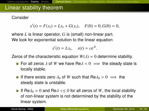
Linear stability theorem
Consider
x′(t) = F(xt) = Lxt + G(xt), F(0) = 0,G(0) = 0,
where L is linear operator, G is (small) non-linear part.We look for exponential solution to the linear equation
x′(t) = Lxt, x(t) = ceλt.
Zeros of the characteristic equation W(λ) = 0 determine stability.
For all zeros λ of W we have Reλ < 0 =⇒ the steady state islocally stable.
If there exists zero λ0 of W such that Reλ0 > 0 =⇒ thesteady state is unstable.
If Reλ0 = 0 and Reλ <≤ 0 for all zeros of W, the local stabilityof non-linear system is not determined by the stability of thelinear system.
Marek Bodnar (MIM) Delay differential equations December 8th, 2016 20 / 39
Gallery of properties Stability Models General theory One equation Two equations More equations or more delays
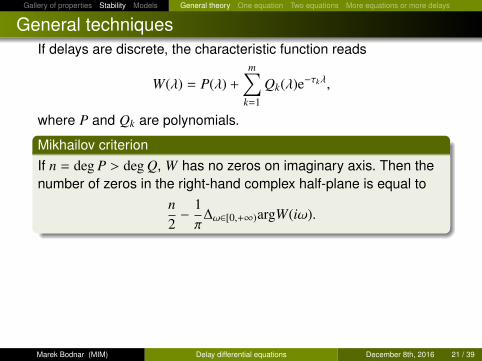
General techniquesIf delays are discrete, the characteristic function reads
W(λ) = P(λ) +
m∑k=1
Qk(λ)e−τkλ,
where P and Qk are polynomials.
Mikhailov criterionIf n = deg P > deg Q, W has no zeros on imaginary axis. Then thenumber of zeros in the right-hand complex half-plane is equal to
n2− 1π
∆ω∈[0,+∞)argW(iω).
Remark
If for τ0k zeros of W crosses imaginary axis (i.e. W(iω0) = 0) that
the same situation is for
τjk = τ0
k +2 jπω0
.
Marek Bodnar (MIM) Delay differential equations December 8th, 2016 21 / 39
Gallery of properties Stability Models General theory One equation Two equations More equations or more delays
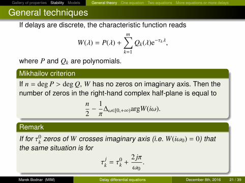
General techniques
In the simplest case, if
W(λ) = P(λ) + Q(λ)e−τλ,
where P and Q are polynomials, we can check if the stabilitychanges. If it is so, there exists purely imaginary zero of W.
W(iω) = P(iω) + Q(iω)e−iτω = 0 =⇒ F(ω) =∣∣∣∣P(iω)
∣∣∣∣2− ∣∣∣∣Q(iω)∣∣∣∣2 = 0.
TheoremUnder some technical assumptions, for F(ω0) = 0.
sign(
ddτ
Re(W(λ)
)∣∣∣∣∣λ=iω0
)= sign
(F′(ω0)
).
K.L. Cooke, P. van den Driessche Funkcj Ekvacioj (1986).
Marek Bodnar (MIM) Delay differential equations December 8th, 2016 22 / 39
Gallery of properties Stability Models General theory One equation Two equations More equations or more delays
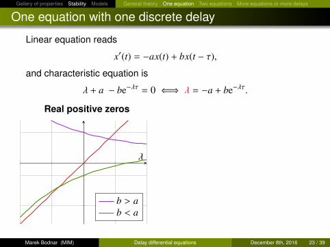
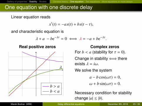
One equation with one discrete delay
Linear equation reads
x′(t) = −ax(t) + bx(t − τ),
and characteristic equation is
λ + a − be−λτ = 0 ⇐⇒ λ = −a + be−λτ.
Real positive zeros
λ
b > ab < a
Complex zerosFor b < a (stability for τ = 0).
Change in stability⇐⇒ thereexists λ = iω.
We solve the system
a − b cos(ωτ) = 0,
ω + b sin(ωτ) = 0.
Necessary condition for stabilitychange |a| ≤ |b|.
Marek Bodnar (MIM) Delay differential equations December 8th, 2016 23 / 39
Gallery of properties Stability Models General theory One equation Two equations More equations or more delays
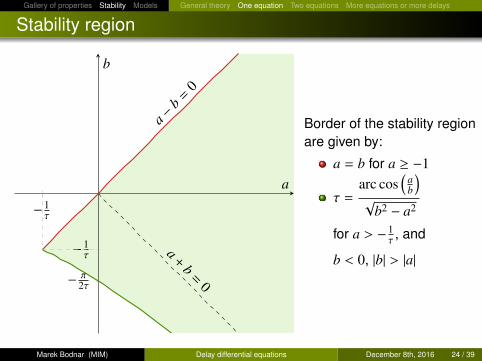
Stability region
−1τ
− π2τ
− 1τ a
+b=
0
a −b =
0
a
b
Border of the stability regionare given by:
a = b for a ≥ −1
τ =arc cos
(ab
)√
b2 − a2
for a > − 1τ , and
b < 0, |b| > |a|
Marek Bodnar (MIM) Delay differential equations December 8th, 2016 24 / 39
Gallery of properties Stability Models General theory One equation Two equations More equations or more delays
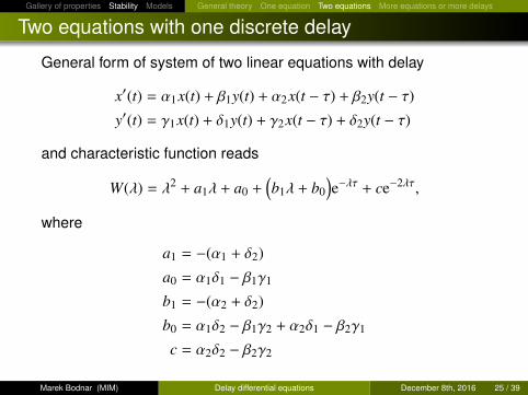
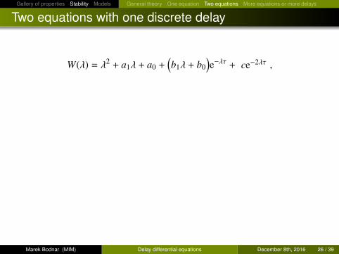
Two equations with one discrete delay
General form of system of two linear equations with delay
x′(t) = α1x(t) + β1y(t) + α2x(t − τ) + β2y(t − τ)
y′(t) = γ1x(t) + δ1y(t) + γ2x(t − τ) + δ2y(t − τ)
and characteristic function reads
W(λ) = λ2 + a1λ + a0 +(b1λ + b0
)e−λτ + ce−2λτ,
where
a1 = −(α1 + δ2)
a0 = α1δ1 − β1γ1
b1 = −(α2 + δ2)
b0 = α1δ2 − β1γ2 + α2δ1 − β2γ1
c = α2δ2 − β2γ2
Marek Bodnar (MIM) Delay differential equations December 8th, 2016 25 / 39
Gallery of properties Stability Models General theory One equation Two equations More equations or more delays
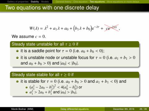
Two equations with one discrete delay
W(λ) = λ2 + a1λ + a0 +(b1λ + b0
)e−λτ + ce−2λτ ,
We assume c = 0.
Steady state unstable for all τ ≥ 0 if
it is a saddle point for τ = 0 (i.e. a0 + b0 < 0);
it is unstable node or unstable focus for τ = 0 (i.e. a1 + b1 > 0and a0 + b0 > 0) and |a0| < |b0|.
Steady state stable for all τ ≥ 0 if
it is stable for τ = 0 (i.e. a0 + b0 > 0 and a1 + b1 < 0) and(a2
1 − 2a0 − b21)2< 4
(a2
0 − b20)
ora2
1 > 2a0 + b21 and |a0| > |b0|.
Marek Bodnar (MIM) Delay differential equations December 8th, 2016 26 / 39
Gallery of properties Stability Models General theory One equation Two equations More equations or more delays
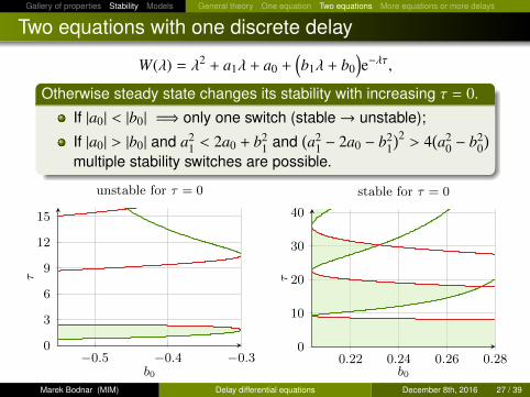
Two equations with one discrete delay
W(λ) = λ2 + a1λ + a0 +(b1λ + b0
)e−λτ,
Otherwise steady state changes its stability with increasing τ = 0.
If |a0| < |b0| =⇒ only one switch (stable→ unstable);
If |a0| > |b0| and a21 < 2a0 + b2
1 and(a2
1 − 2a0 − b21)2 > 4
(a2
0 − b20)
multiple stability switches are possible.
−0.5 −0.4 −0.30
3
6
9
12
15
b0
τ
unstable for τ = 0
0.22 0.24 0.26 0.280
10
20
30
40
b0
τ
stable for τ = 0
Marek Bodnar (MIM) Delay differential equations December 8th, 2016 27 / 39
Gallery of properties Stability Models General theory One equation Two equations More equations or more delays
More equations or more delays
Situation can be more complex.
Even for one equation and two discrete delays multiplestability changes are possible.
If delay distribution is continuous, that is delay term is writtenas ∫ +∞
0θ(s)x(t − s)ds,
where θ is a probabilistic density on [0,+∞), then in thecharacteristic function Laplace transform of θ can be involved.
Marek Bodnar (MIM) Delay differential equations December 8th, 2016 28 / 39
Gallery of properties Stability Models Hutchinson model Gene expression with negative feedback
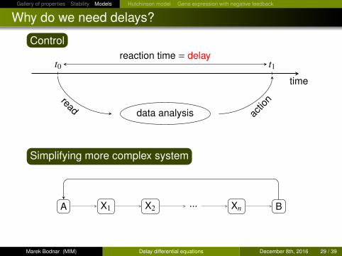
Why do we need delays?
Control
time
data analysisread
actio
n
t0 t1reaction time = delay
Simplifying more complex system
A X1 X2 ... Xn B
time of many process = delay
Marek Bodnar (MIM) Delay differential equations December 8th, 2016 29 / 39
Gallery of properties Stability Models Hutchinson model Gene expression with negative feedback
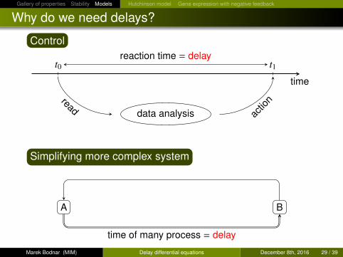
Why do we need delays?
Control
time
data analysisread
actio
n
t0 t1reaction time = delay
Simplifying more complex system
A
X1 X2 ... Xn
B
time of many process = delay
Marek Bodnar (MIM) Delay differential equations December 8th, 2016 29 / 39

Gallery of properties Stability Models Hutchinson model Gene expression with negative feedback
Where does time delay appear?
In models ofbiological processes eg.
tumour growth and cancer therapies,
biochemical reactions and gene expression,
immune system,
spread of epidemic,
economic processes eg.optimisation of fishing,
controlling of pollutions,
physical and chemical processes eg.lasers,
sociological processes.
Marek Bodnar (MIM) Delay differential equations December 8th, 2016 30 / 39
Gallery of properties Stability Models Hutchinson model Gene expression with negative feedback
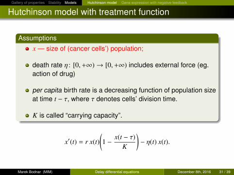
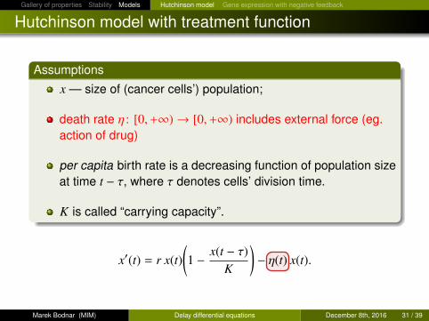
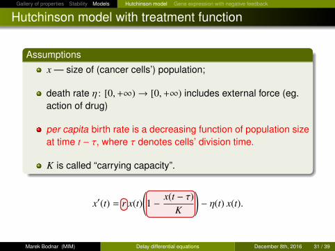
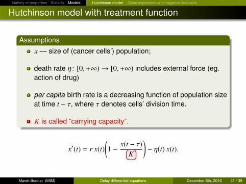
Hutchinson model with treatment function
Assumptions
x — size of (cancer cells’) population;
death rate η : [0,+∞)→ [0,+∞) includes external force (eg.action of drug)
per capita birth rate is a decreasing function of population sizeat time t − τ, where τ denotes cells’ division time.
K is called “carrying capacity”.
x′(t) = r x(t)(1 − x(t − τ)
K
)− η(t) x(t).
Marek Bodnar (MIM) Delay differential equations December 8th, 2016 31 / 39
Gallery of properties Stability Models Hutchinson model Gene expression with negative feedback
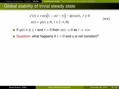
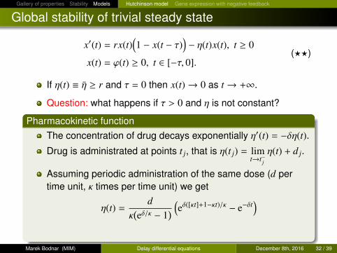
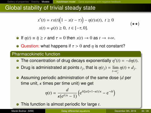
Global stability of trivial steady state
x′(t) = rx(t)(1 − x(t − τ)
)− η(t)x(t), t ≥ 0
x(t) = ϕ(t) ≥ 0, t ∈ [−τ, 0].(??)
If η(t) ≡ η ≥ r and τ = 0 then x(t)→ 0 as t → +∞.
Question: what happens if τ > 0 and η is not constant?
Pharmacokinetic functionThe concentration of drug decays exponentially η′(t) = −δη(t).
Drug is administrated at points t j, that is η(t j) = limt→t−j
η(t) + d j.
Assuming periodic administration of the same dose (d pertime unit, κ times per time unit) we get
η(t) =d
κ(eδ/κ − 1
) (eδ([κt]+1−κt)/κ − e−δt
)
This function is almost periodic for large t.
Marek Bodnar (MIM) Delay differential equations December 8th, 2016 32 / 39
Gallery of properties Stability Models Hutchinson model Gene expression with negative feedback
Global stability of trivial steady state
x′(t) = rx(t)(1 − x(t − τ)
)− η(t)x(t), t ≥ 0
x(t) = ϕ(t) ≥ 0, t ∈ [−τ, 0].(??)
If η(t) ≡ η ≥ r and τ = 0 then x(t)→ 0 as t → +∞.
Question: what happens if τ > 0 and η is not constant?
Pharmacokinetic functionThe concentration of drug decays exponentially η′(t) = −δη(t).
Drug is administrated at points t j, that is η(t j) = limt→t−j
η(t) + d j.
Assuming periodic administration of the same dose (d pertime unit, κ times per time unit) we get
η(t) =d
κ(eδ/κ − 1
) (eδ([κt]+1−κt)/κ − e−δt
)This function is almost periodic for large t.
Marek Bodnar (MIM) Delay differential equations December 8th, 2016 32 / 39
Gallery of properties Stability Models Hutchinson model Gene expression with negative feedback
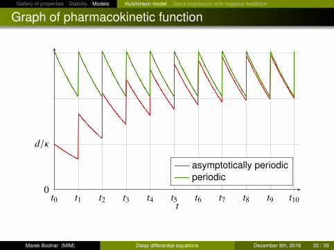
Graph of pharmacokinetic function
t0 t1 t2 t3 t4 t5 t6 t7 t8 t9 t100
d/κ
t
asymptotically periodicperiodic
Marek Bodnar (MIM) Delay differential equations December 8th, 2016 33 / 39
Gallery of properties Stability Models Hutchinson model Gene expression with negative feedback
Global stability of the steady state
Generalised equationx′(t) = rx(t) f
(x(t − τ)
)− η(t)x(t), (??)
f is strictly decreasing, f (1) = 0, andf (0) = 1 or limx→0+ f (x) = +∞.η is asymptotically periodic, i.e. η(t) = ηp(t) + ηr(t), where ηp isperiodic with period σ, ηr(t)→ 0 as t → +∞.∫ +∞
0ηr(t)dt is convergent.
TheoremUnder the above assumptions the trivial steady state of (??) isglobally stable if and only if
1σ
∫ σ
0η(t)dt ≥ lim
x→0+f (x).
M.B., U. Forys, M.J. Piotrowska, Appl. Math. Lett., (2013).
Marek Bodnar (MIM) Delay differential equations December 8th, 2016 34 / 39
Gallery of properties Stability Models Hutchinson model Gene expression with negative feedback
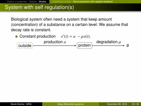
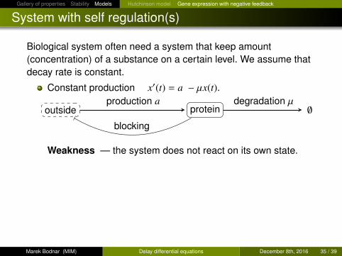
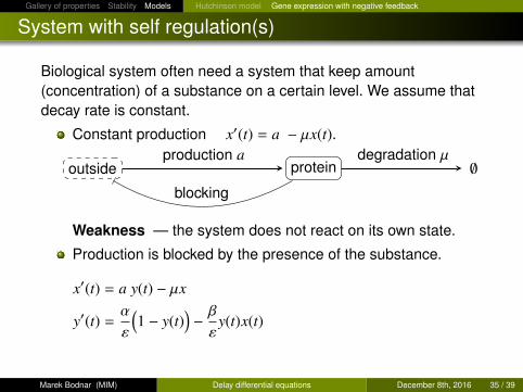
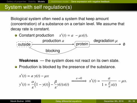
System with self regulation(s)
Biological system often need a system that keep amount(concentration) of a substance on a certain level. We assume thatdecay rate is constant.
Constant production
x′(t) = a − µx(t).
outside protein ∅production a degradation µ
blocking
Weakness — the system does not react on its own state.
Production is blocked by the presence of the substance.
x′(t) = a y(t) − µx
y′(t) =α
ε
(1 − y(t)
)− βε
y(t)x(t)
ε→0========⇒ x′(t) =
a
1 +βα x(t)
− µx.
Marek Bodnar (MIM) Delay differential equations December 8th, 2016 35 / 39
Gallery of properties Stability Models Hutchinson model Gene expression with negative feedback
System with self regulation(s)
Biological system often need a system that keep amount(concentration) of a substance on a certain level. We assume thatdecay rate is constant.
Constant production x′(t) = a − µx(t).
outside protein ∅production a degradation µ
blocking
Weakness — the system does not react on its own state.
Production is blocked by the presence of the substance.
x′(t) = a y(t) − µx
y′(t) =α
ε
(1 − y(t)
)− βε
y(t)x(t)
ε→0========⇒ x′(t) =
a
1 +βα x(t)
− µx.
Marek Bodnar (MIM) Delay differential equations December 8th, 2016 35 / 39
Gallery of properties Stability Models Hutchinson model Gene expression with negative feedback
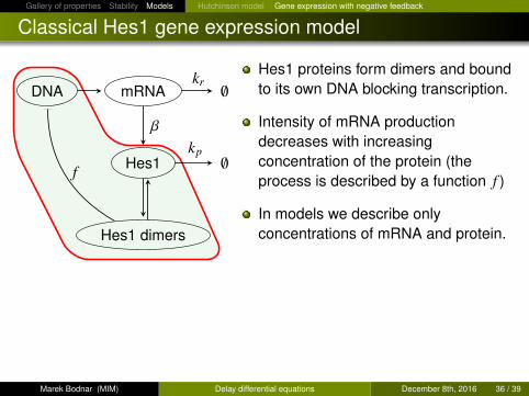
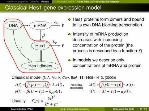
Classical Hes1 gene expression model
DNA mRNA
Hes1
Hes1 dimers
f
kr ∅
kp ∅
β
Hes1 proteins form dimers and boundto its own DNA blocking transcription.
Intensity of mRNA productiondecreases with increasingconcentration of the protein (theprocess is described by a function f )
In models we describe onlyconcentrations of mRNA and protein.
Classical model (N.A. Monk, Curr. Biol., 13: 1409–1413, (2003))
r(t) = f (p(t − τr)) − krr(t) ,
p(t) = βr(t − τp) − kp p(t) ,
rescaling======⇒ x(t) = f (y(t − τ1)) − x(t) ,
y(t) = x(t − τ2) − µy(t) ,
Usually f (p) =γrkh
kh + ph .
Marek Bodnar (MIM) Delay differential equations December 8th, 2016 36 / 39
Gallery of properties Stability Models Hutchinson model Gene expression with negative feedback
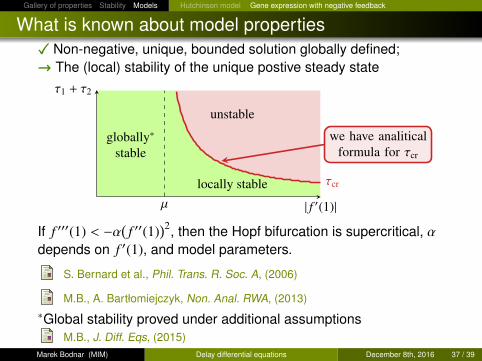
What is known about model propertiesX Non-negative, unique, bounded solution globally defined;→ The (local) stability of the unique postive steady state
| f ′(1)|
τ1 + τ2
µ
locally stable
unstable
globally∗
stablewe have analitical
formula for τcr
τcr
If f ′′′(1) < −α( f ′′(1))2, then the Hopf bifurcation is supercritical, α
depends on f ′(1), and model parameters.
S. Bernard et al., Phil. Trans. R. Soc. A, (2006)
M.B., A. Bartłomiejczyk, Non. Anal. RWA, (2013)∗Global stability proved under additional assumptions
M.B., J. Diff. Eqs, (2015)Marek Bodnar (MIM) Delay differential equations December 8th, 2016 37 / 39
Gallery of properties Stability Models Hutchinson model Gene expression with negative feedback
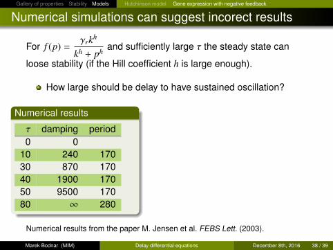
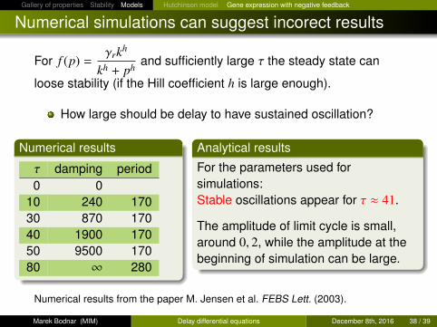
Numerical simulations can suggest incorect results
For f (p) =γrkh
kh + ph and sufficiently large τ the steady state can
loose stability (if the Hill coefficient h is large enough).
How large should be delay to have sustained oscillation?
Numerical results
τ damping period0 0
10 240 17030 870 17040 1900 17050 9500 17080 ∞ 280
Analytical results
For the parameters used forsimulations:Stable oscillations appear for τ ≈ 41.
The amplitude of limit cycle is small,around 0, 2, while the amplitude at thebeginning of simulation can be large.
Numerical results from the paper M. Jensen et al. FEBS Lett. (2003).
Marek Bodnar (MIM) Delay differential equations December 8th, 2016 38 / 39
Gallery of properties Stability Models Hutchinson model Gene expression with negative feedback
Numerical simulations can suggest incorect results
For f (p) =γrkh
kh + ph and sufficiently large τ the steady state can
loose stability (if the Hill coefficient h is large enough).
How large should be delay to have sustained oscillation?
Numerical results
τ damping period0 0
10 240 17030 870 17040 1900 17050 9500 17080 ∞ 280
Analytical results
For the parameters used forsimulations:Stable oscillations appear for τ ≈ 41.
The amplitude of limit cycle is small,around 0, 2, while the amplitude at thebeginning of simulation can be large.
Numerical results from the paper M. Jensen et al. FEBS Lett. (2003).
Marek Bodnar (MIM) Delay differential equations December 8th, 2016 38 / 39

Gallery of properties Stability Models Hutchinson model Gene expression with negative feedback
Current projects (of M.B. U. Forys and M.J. Piotrowska)
Currently we are working on mathematical models of tumour, inparticular brain tumour in the framework of
Mathematical models and methods in description of tumourgrowth and its therapies. (NCN, OPUS),
Therapy optimization in glioblastoma: An integrative humandata-based approach using mathematical models (James S.Mc. Donnell Foundation), PI: Victor Perez Garcia.This is a collaborative project in which many institution areinvolved, among others
Mathematical Oncology Laboratory, Universidad de Castilla-LaMancha, Spain
Hospital 12 de Octubre, Madrid, Spain
Fundación Hospital de Madrid, HM Hospitals, Spain
Department of Neurobiology, Institute for Biological Research,University of Belgrade, Serbia
Bern Inselspital, Switzerland.Marek Bodnar (MIM) Delay differential equations December 8th, 2016 39 / 39

Thank you for your attention!Thank you for your attention!
Recommended