DIFFERENTIAL ANALYSIS OF FLUID FLOW
A: Mathematical Formulation (4.1.1, 4.2, 6.1-6.4)
B: Inviscid Flow: Euler Equation/Some Basic, Plane Potential Flows (6.5-6.7)
C: Viscous Flow: Navier-Stokes Equation (6.8-6.10)

IntroductionDifferential AnalysisDifferential Analysis
There are situations in which the details of the flow are important, e.g., pressure and shear stress variation along the wing….Therefore, we need to develop relationship that apply at a point or at least in a very small region (infinitesimal volume) with a given flow field.This approach is commonly referred to as differential analysis.The solutions of the equations are rather difficult.Computational Fluid Dynamic (CFD) can be applied to complex flow problems.

PART AMathematical Formulation
(Sections 4.1.1, 4.2, 6.1-6.4)

Fluid Kinematics (4.1.1, 4.2)Fluid Kinematics (4.1.1, 4.2)
Kinematics involves position, velocity and acceleration, not forces.kinematics of the motion: velocity and acceleration of the fluid, and the description and visualization of its motion.The analysis of the specific force necessary to produce the motion - the dynamics of the motion.

4.1 The Velocity FieldA field representation – representations of fluid parameters as functions of spatial coordinate
the velocity field
( ) ( ) ( )ktzyxwjtzyxvitzyxuV ,,,,,,,,, ++=A
Adr Vdt
=r uur
( )tzyxVV ,,,=
( ) 21222 wvuVV ++==
A change in velocity results in an acceleration which may be due to a change in speed and/or direction.

4.1.1 Eulerian and LagrangianFlow DescriptionsEulerian method: the fluid motion is given by completely prescribing the necessary properties as functions of space and time.
From this method, we obtain information about the flow in terms of what happens at fixed points in space as the fluid flows past those points.
Lagrangian method: following individual fluid particles as they move about and determining how the fluid properties associated with these particles change as a function of time. V4.3 Cylinder-velocity vectors
V4.4 Follow the particlesV4.5 Follow the particles

4.1.4 Streamlines, Streaklines and Pathlines
A streamline is a line that is everywhere tangent to the velocity field.A streakline consists of all particles in a flow that have previously passed through a common point.A pathline is a line traced out by a given flowing particle.
V4.9 streamlinesV4.10 streaklinesV4.1 streaklines

4.1.4 Streamlines, Streaklines and PathlinesFor steady flows, streamlines, streaklines and pathlines all coincide. This is not true for unsteady flows.
Unsteady streamlines are difficult to generate experimentally, but easy to draw in numerical computation.On the contrary, streaklines are more of a lab tool than an analytical tool.How can you determine the unsteady pathline of a moving particle?

4.2 The Acceleration Field
The acceleration of a particle is the time rate change of its velocity.For unsteady flows the velocity at a given point in space may vary with time, giving rise to a portion of the fluid acceleration.In addition, a fluid particle may experience an acceleration because its velocity changes as it flows from one point to another in space.

4.2.1 The Material Derivative
Consider a particle moving along its pathline
( ) ( ) ( ) ( ), , , ,A A A A A A AV V r t V x t y t z t t= = ⎡ ⎤⎣ ⎦uur uur ur uur

The Material Derivative
Thus the acceleration of particle A,
( ) ( ) ( ) ( )
( )
, , , ,
=
A A A A A A A
A A A A A AA
A A
A A A AA A A
V V r t V x t y t z t t
dV V V dx V dya tdt t x dt y dt
V dzz dt
V V V Vu v wt x y z
= = ⎡ ⎤⎣ ⎦
∂ ∂ ∂= = + +
∂ ∂ ∂
∂+
∂∂ ∂ ∂ ∂
+ + +∂ ∂ ∂ ∂
uur uur ur uur
uur uur uur uuruur
uur
uur uur uur uur

Acceleration
This is valid for any particle
x
y
z
V V V Va u v wt x y zu u u ua u v wt x y zv v v va u v wt x y zw w w wa u v wt x y z
∂ ∂ ∂ ∂= + + +
∂ ∂ ∂ ∂∂ ∂ ∂ ∂
= + + +∂ ∂ ∂ ∂∂ ∂ ∂ ∂
= + + +∂ ∂ ∂ ∂∂ ∂ ∂ ∂
= + + +∂ ∂ ∂ ∂
ur ur ur urr

Material derivativeAcceleration:
Total derivative, material derivative or substantial derivative
( ) ( ) ( ) ( ) ( )
( ) ( ) = ( )
Du v w
Dt t x y z
Vt
∂ ∂ ∂ ∂= + + +
∂ ∂ ∂ ∂
∂+ ⋅∇
∂
r
, DV DV V V V Va u v wDt Dt t x y z
∂ ∂ ∂ ∂= = + + +
∂ ∂ ∂ ∂
ur ur ur ur ur urr
Associated with time variation
Associated with space variation

Material derivativeThe material derivative of any variable is the rate at which that variable changes with time for a given particle (as seen by one moving along with the fluid – the Lagrangiandescriptions)If velocity is known, the time rate change of temperature can be expressed as,
= ( )
DT T T T Tu v wDt t x y z
T V Tt
∂ ∂ ∂ ∂= + + +
∂ ∂ ∂ ∂∂
+ ⋅∇∂
r
Example: the temperature of a passenger experienced on a train starting from Taipei on 9am and arriving at Kaohsiung on 12.

Acceleration along a streamline
33 4
3(1 ) [ ( 3 )] o oRa V V R x ix
−= + −r r
( )3
0 3 1 , R V V u uV u x i V i a u u ix t x t x
⎛ ⎞ ∂ ∂ ∂ ∂⎛ ⎞= = + = + = +⎜ ⎟ ⎜ ⎟∂ ∂ ∂ ∂⎝ ⎠⎝ ⎠
ur urur r r r r

4.2.2 Unsteady EffectsFor steady flow ( )/ 0, there is no change in flow parameters at a fixed point in space.For unsteady flow ( )/ 0.
spatial (convective) derivative
t
t
DT T VDt t
∂ ∂ ≡
∂ ∂ ≠
↓∂
= + ⋅∇∂
v (for an unstirred cup of coffee 0)
time (local) derivative
local acceleration
DT TTDt t
DV V V VDt t
∂→ <
∂↑
∂= + ⋅∇
∂↑
v vv v
V4.12 Unsteady flow

4.2.3 Convective Effects
0
=0+
s
out ins
DT T V TDt tDT TuDt s
T Tus
∂= + ⋅∇
∂∂
= +∂
−Δ
v

4.2.3 Convective Effects
convective acceleration
local acceleration
0
DV V V VDt t
Du uuDt x
↓
∂= + ⋅∇
∂↑
∂= +
∂
v vv v

4.2.4 Streamline CoordinatesIn many flow situations it is convenient to use a coordinate system defined in terms of the streamlines of the flow.
V V sDV DV Dsa s VDt Dt Dt
V V ds V dn st s dt n dt
s s ds s dnVt s dt n dt
=
= = +
∂ ∂ ∂⎛ ⎞= + +⎜ ⎟∂ ∂ ∂⎝ ⎠∂ ∂ ∂⎛ ⎞+ + +⎜ ⎟∂ ∂ ∂⎝ ⎠
v v
v vv v
v
v v v
V4.13 Streamline coordinates

4.2.4 Streamline Coordinates
2 2
0
Steady flow
or ,
1 , or , lim
s n
s
V sa V s V Vs s
V V V VV s n a V as R s R
ss s s s nsR s s R s s Rδ
δδ δ δδδ δ→
∂ ∂⎛ ⎞ ⎛ ⎞= +⎜ ⎟ ⎜ ⎟∂ ∂⎝ ⎠ ⎝ ⎠∂ ∂
= + = =∂ ∂
⎛ ⎞∂= = = = =⎜ ⎟⎜ ⎟∂⎝ ⎠
vv v
v v
v v v v vv
Q v

6.1 Fluid Element Kinematics
Types of motion and deformation for a fluid element.

6.1.1 Velocity and Acceleration Fields Revisited
Velocity field representation
Acceleration of a particle( ), , , or V V x y z t V ui v j wk= = + +
ur ur ur r r r
zVw
yVv
xVu
tVa
∂∂
+∂∂
+∂∂
+∂∂
=
zuw
yuv
xuu
tuax ∂
∂+
∂∂
+∂∂
+∂∂
=
zvw
yvv
xvu
tvay ∂
∂+
∂∂
+∂∂
+∂∂
=
zww
ywv
xwu
twaz ∂
∂+
∂∂
+∂∂
+∂∂
=
( )
( ) ( ) ( ) ( )
DV Va V VDt t
i j kx y z
∂= = + ∇
∂∂ ∂ ∂
∇ = + +∂ ∂ ∂
ur urr ur ur
r r r

variations of the velocity in the direction of velocity, , , cause a linear stretchingdeformation.Consider the x-component deformation:
6.1.2 Linear Motion and Deformation
xu
∂∂
yv
∂∂
zw
∂∂

( )0
Rate change of per unit volume due to / :
/1 ( ) limt
V u x
u x td V uV dt t xδ
δ
δδδ δ→
∂ ∂
⎡ ⎤∂ ∂ ∂= =⎢ ⎥ ∂⎣ ⎦
The change in the original volume, , due to / :
Change in ( )( )( )
V x y z u xuV x y z tx
δ δ δ δ
δ δ δ δ δ
= ∂ ∂∂
=∂
If velocity gradient / and / are also present, then1 ( )
v y w zd V u v w V
V dt x y zδ
δ
∂ ∂ ∂ ∂∂ ∂ ∂
= + + = ∇ ⋅ ←∂ ∂ ∂
volumetric dilatation rateuv
Linear Motion and Deformation
The volume of a fluid may change as the element moves from one location to another in the flow field. For incompressible fluid, the volumetric dilation rate is zero.

6.1.3 Angular Motion and Deformation
Consider an element under rotation and angular deformation
V6.3 Shear deformation

the angular velocity of OA is
For small angles
0OA tlim
tδ
δαωδ→
=
tan
v x t vx tx x
δ δδα δα δ
δ
∂∂∂≈ = =∂
so that
0
( / )OA t
v x t vlimt xδ
δ δ δ δωδ δ→
⎡ ⎤= =⎢ ⎥⎣ ⎦
(if is positive then will be counterclockwise) xv
∂∂
OAω
Angular Motion and Deformation

the angular velocity of the line OB is
0OB tlim
tδ
δβωδ→
=
tyu
y
tyyu
δδ
δδδβδβ
∂∂
=∂∂
=≈tan
so that
( )0
/limOB t
u y t ut yδ
δω
δ→
⎡ ⎤∂ ∂ ∂= =⎢ ⎥ ∂⎣ ⎦
( if is positive, will be clockwise)yu
∂∂
OBω
Angular Motion and Deformation

Angular rotation
The rotation, , of the element about the z axis is defined as the average of the angular velocities and , if counterclockwise is considered to be positive, then,
zωOAω OBω
⎟⎟⎠
⎞⎜⎜⎝
⎛∂∂
−∂∂
=yu
xv
z 21ω
similarly
⎟⎟⎠
⎞⎜⎜⎝
⎛∂∂
−∂∂
=zv
yw
x 21ω ⎟
⎠⎞
⎜⎝⎛
∂∂
−∂∂
=xw
zu
y 21ω
,
thus
kyu
xvj
xw
zui
zv
yw
wvuzyx
kji
V ⎟⎟⎠
⎞⎜⎜⎝
⎛∂∂
−∂∂
+⎟⎠⎞
⎜⎝⎛
∂∂
−∂∂
+⎟⎟⎠
⎞⎜⎜⎝
⎛∂∂
−∂∂
=∂∂
∂∂
∂∂
=×∇21
21
21
21
21
VVcurlkji xyx
rrrrrr×∇==++=
21
21ωωωω
V4.6 Flow past a wing

Define vorticity
If or , then the rotation (and the vorticity )
are zero, and flow fields are termed irrotational.
ξ
V×∇== ωξ 2
The fluid element will rotate about z axis as an undeformedblock ( ie: ) OBOA ωω −=
only when xv
yu
∂∂
−=∂∂
xv
yu
∂∂
=∂∂
0=×∇ V
Otherwise the rotation will be associated with an angular deformation.
Definition of vorticity

Different types of angular motions
Solid body rotation
Free vortex
ru Ω=φ 0== zr uu
Ω= 2zω 0== φωω r
( )θ
ω φ ∂∂
−∂∂
= rz
ur
rurr
11
rku =φ 0== zr uu
0=φω 0=rω
( ) 01=
∂∂
= φω rurrz 0≠rfor

Apart form rotation associated with these derivatives and , these derivatives can cause the element to undergo an angular deformation, which results in a changein shape of the element.
The change in the original right angle is termed the shearing strain ,
where is considered to be positive if the original right angle is decreasing.
yu
∂∂
xv
∂∂
δγδβδαδγ +=
δγ
Angular Deformation

Rate of shearing strain or rate of angular deformation
0 0lim limt t
v ut tx y
t t
v ux y
δ δ
δ δδγγδ δ→ →
∂ ∂⎡ ⎤+⎢ ⎥∂ ∂= = ⎢ ⎥⎢ ⎥⎢ ⎥⎣ ⎦
∂ ∂= +
∂ ∂
&
The rate of angular deformation is related to a corresponding shearing stress which causes the fluid element to change in shape.
If , the rate of angular deformation is zero and this condition indicates that the element is simply rotating as an undeformed block.
xv
yu
∂∂
−=∂∂
Angular Deformation

6.2 Conservation of Mass
0=Dt
DM sys
0=•+∂∂
∫∫ cscvdAnVVd
tρρ
Conservation of mass:
In control volume representation (continuity equation):
(6.19)
To obtain the differential form of the continuity equation, Eq. 6.19 is applied to an infinitesimal control volume.

6.2.1 Differential Form of Continuity Equation
zyxt
Vdt
δδδρρ∂∂
≡∂∂
∫Net mass flow in the direction zyx
xuzyx
xuuzyx
xuu δδδρδδδρρδδδρρ
∂∂
=⎥⎦⎤
⎢⎣⎡
∂∂
−−⎥⎦⎤
⎢⎣⎡
∂∂
+22
Net mass flow in the y direction zyxyv δδδ
ρρ∂
Net mass flow in the z direction zyxzw δδδ
ρρ∂
Net rate of mass out of flow zyxzw
yv
xu δδδρρρ
⎥⎦
⎤⎢⎣
⎡∂
∂+
∂∂
+∂
∂

Differential Form of Continuity Equation
Thus conservation of mass become
In vector form
For steady compressible flow
For incompressible flow
0=⋅∇ Vr
0=∂
∂+
∂∂
+∂
∂+
∂∂
zw
yv
xu
tρρρρ (continuity equation )
0=∂
∂+
∂∂
+∂
∂zw
yv
xu ρρρ
0=∂∂
+∂∂
+∂∂
zw
yv
xu
0=⋅∇ Vr
ρ
0=⋅∇+∂∂ V
t
rρρ

6.2.2 Cylindrical Polar Coordinates
The differential form of continuity equation
( ) ( )011
=∂
∂+
∂∂
+∂
∂+
∂∂
zvv
rrvr
rtzr ρ
θρρρ θ

For 2-D incompressible plane flow then,
Define a stream function such that
For velocity expressed in forms of the stream function, the conservation of mass will be satisfied.
6.2.3 The Stream Function
0=∂∂
+∂∂
yv
xu
( ),x yψ
uyψ∂
=∂
vxψ∂
= −∂
then2 2
0x y x y x y y x
ψ ψ ψ ψ⎛ ⎞ ⎛ ⎞∂ ∂ ∂ ∂ ∂ ∂+ − = − =⎜ ⎟ ⎜ ⎟∂ ∂ ∂ ∂ ∂ ∂ ∂ ∂⎝ ⎠ ⎝ ⎠

The Stream Function
Lines along constant are stream lines.Definition of stream line
Thus we can use to plot streamline.The actual numerical value of a stream line is not important butthe change in the value of is related to the volume flow rate.
ψ
uv
dxdy
=
Thus change of , from to
0dψ =
0=+− udyvdxuv
dxdy
=
which is the defining equation for a streamline.
ψ
ψ
Along a line of constant of we have
( , )x y ( , )x dx y dy+ +
ψ
ψ
udyvdxdyy
dxx
d +−=∂∂
+∂∂
=ψψψ

Note:Flow never crosses streamline, since by definition the velocity is tangent to the streamlines.
Volume rate of flow (per unit width perpendicular to the x-yplane)
In cylindrical coordinates the incompressible continuity equation becomes,
2
12 1
dq udy vdx
dy dx dy x
q dψ
ψ
ψ ψ ψ
ψ ψ ψ
= −∂ ∂
= + =∂ ∂
= = −∫
2 1ψ ψ>If then q is positive and vice versa.
( )011
=∂∂
+∂
∂θθv
rrrv
rr
Then,1
rvr
ψθ
∂=
∂v
rθψ∂
= −∂
The Stream Function
Ex 6.3 Stream function

6.3 Conservation of Linear Momentum
Linear momentum equation
Consider a differential system with and
Using the system approach then
∫=sys
dmVDtDF
or
mδ Vδ
amDtVDmF δδδ ==
then ( )Dt
mVDF δδ =
dAnVVVdVt
FCSCV
rrrrr⋅+
∂∂
= ∫∫∑ ρρ volumecontrol
theof contents

6.3.1 Descriptions of Force Acting on theDifferential Element
Two types of forces need to be considered surface forces:which action the surfaces of the
differential element.body forces:which are distributed throughout the
element.
For simplicity, the only body force considered is the weight of the element,
or
bF mgδ δ=ur ur
xbx mgF δδ = yby mgF δδ = zbz mgF δδ =

Surface force act on the element as a result of its interaction with its surroundings (the components depend on the area orientation)
nFδ Aδ 1Fδ 2FδWhere is normal to the area and and are parallel to the area and orthogonal to each other.

The normal stress is defined as,
Sign of stresses
nσ
AFn
An δδ
σδ 0lim
→=
and the shearing stresses are define as
AF
A δδ
τδ
1
01 lim→
=AF
A δδ
τδ
2
02 lim→
=
we use for normal stresses and for shear stresses.σ τ
Note:Positive normal stresses are tensile stresses, ie, they tend to stretch the material.
Positive sign for the stress as positive coordinate directionon the surfaces for which the outward normal is in the positive coordinate direction.

Thus yxxx zxsx
xy yy zysy
yxxz zzsz
F x y zx y z
F x y zx y z
F x y zx y z
τσ τδ δ δ δ
τ σ τδ δ δ δ
ττ σδ δ δ δ
∂⎛ ⎞∂ ∂= + +⎜ ⎟∂ ∂ ∂⎝ ⎠
∂ ∂ ∂⎛ ⎞= + +⎜ ⎟∂ ∂ ∂⎝ ⎠
∂⎛ ⎞∂ ∂= + +⎜ ⎟∂ ∂ ∂⎝ ⎠
s sx sy sz
s b
F F i F j F k
F F F
δ δ δ δ
δ δ δ
= + +
= +
ur r r r
ur uur uur

6.3.2 Equation of Motion
zyxm δδρδδ =
Thus
y xx x z xx
x y y y zyy
y zx z z zz
u u u ug u v wx y z t x y z
v v v vg u wvx y z t x y z
w w w wg u v wx y z t x y z
τσ τρ ρ
τ σ τρ ρ
ττ σρ ρ
∂ ⎛ ⎞∂ ∂ ∂ ∂ ∂ ∂+ + + = + + +⎜ ⎟∂ ∂ ∂ ∂ ∂ ∂ ∂⎝ ⎠
∂ ∂ ∂ ⎛ ⎞∂ ∂ ∂ ∂+ + + = + + +⎜ ⎟∂ ∂ ∂ ∂ ∂ ∂ ∂⎝ ⎠
∂ ⎛ ⎞∂ ∂ ∂ ∂ ∂ ∂+ + + = + + +⎜ ⎟∂ ∂ ∂ ∂ ∂ ∂ ∂⎝ ⎠
(6.50)
zzyyxx amFamFamF δδδδδδ ===rrr
,,

PART BInviscid Flow:
Euler Equation/Some Basic, Plane Potential Flows
(Sections 6.5-6.7)

For an inviscid flow in which the shearing stresses are all zero, and the normal stresses are replaced by -p, thus the equation of motion becomes
The main difficulty in solving the equation is the nonlinear terms which appear in the convective acceleration.
( )
x
y
z
p u u u ug u wx t x y z
pg u wy t x y z
p w w w wg u wz t x y z
or
Vg p V Vt
ρ ρ υ
υ υ υ υρ ρ υ
ρ ρ υ
ρ ρ
⎛ ⎞∂ ∂ ∂ ∂ ∂− = + + +⎜ ⎟∂ ∂ ∂ ∂ ∂⎝ ⎠
⎛ ⎞∂ ∂ ∂ ∂ ∂− = + + +⎜ ⎟∂ ∂ ∂ ∂ ∂⎝ ⎠
⎛ ⎞∂ ∂ ∂ ∂ ∂− = + + +⎜ ⎟∂ ∂ ∂ ∂ ∂⎝ ⎠
⎡ ⎤∂− ∇ = + ⋅∇⎢ ⎥∂⎣ ⎦
uvuv uvv
6.4 Inviscid Flow6.4.1 Euler’s Equation of Motion

For steady flow
Take the dot product of each term with a differential length ds along a streamline
thus the equation can be written as,
6.4.2 The Bernoulli Equation
( )
( ) ( ) ( )(up being positive)
12
g p V V
g g z
V V V V V V
ρ ρ− ∇ = ⋅∇
= − ∇
⋅∇ = ∇ ⋅ − × ∇×
uv uvv
uv
uv uv uv uv uv uv
( ) ( )
( ) ( )2
2or
12
g z p V V V V
p V g z V V
ρρ ρ
ρ
− ∇ − ∇ = ∇ ⋅ − × ∇×
∇+ ∇ + ∇ = × ∇×
uv uv uv uv
uv uv
( ) ( )212
p d s V d s g z d s V V d sρ
∇ ⎡ ⎤⋅ + ∇ ⋅ + ∇ ⋅ = × ∇× ⋅⎣ ⎦v v v uv uv v

Since and are parallel, therefore
Since
d sv
Vuv
( ) 0V V ds⎡ ⎤× ∇× ⋅ =⎣ ⎦uv v v
d s dx i dy j dz kp p pp d s dx dy dz dpx y z
= + +∂ ∂ ∂
∇ ⋅ = + + =∂ ∂ ∂
v v vv
v
Thus the equation becomes
( )21 02
dp d V g dzρ
+ + =
where the change in and z is along the streamline , ,p Vuv

Equation after integration become2
constant2
dp V gzρ
+ + =∫which indicates that the sum of the three terms on the left side of the equation must remain a constant along a given streamline.
For inviscid, incompressible flow, the equation become, 2
2 21 1 2 2
1 2
const2
or
2 2
p V gz
p V p Vz zg g
ρ
γ γ
+ + =
+ + = + +
※ For (1) inviscid flow(2) steady flow(3) incompressible flow(4) flow along a streamline

6.4.3 Irrotational FlowIf the flow is irrotational, the analysis of inviscid flow problem is further simplified.The rotation of the fluid element is equal to , and for irrotational flow field,
Since , therefore for an irrotational
flow field, the vorticity is zero.
Vr
×∇21
0V∇× =uv
V ζ∇× =uv uv
ωr
The condition of irrotationality imposes specific relationships among these velocity gradients. For example,
A general flow field would not satisfy these three equations.
1 02
, ,
zu
x yu w u w
x y y z z x
υω
υ υ
⎛ ⎞∂ ∂= − =⎜ ⎟∂ ∂⎝ ⎠
∂ ∂ ∂ ∂ ∂ ∂= = =
∂ ∂ ∂ ∂ ∂ ∂

Can irrotational flow hold in a viscous fluid?
According to the 2-D vorticity transport equation (cf. Problem 6.81)
Vorticity of an fluid element grows along with its motion as long as ν is positive. So, an initially irrotatioal flow will eventually turn into rotational flow in a viscous fluid.On the other hand, an initially irrotatioal flow remains irrotational in an inviscid fluid, if without external excitement.
2zz
DDtζ ν ζ= ∇

In Section 6.4.2, we have obtained along a streamline that,
Consequently, for irrotational flow the Bernoulli equation is valid throughout the flow field. Therefore, between any flow points in the flow field,
6.4.4 The Bernoulli Equation for Irrotational Flow
( ) 0V V ds⎡ ⎤× ∇× ⋅ =⎣ ⎦uv uv
0V∇× =uv
2
2 21 1 2 2
1 2
constant2or
2 2
dp V gz
p V p Vz zg g
ρ
γ γ
+ + =
+ + = + +
∫
In an irrotational flow, , so the equation is zero regardless of the direction of .d sv
※ For (1) Inviscid flow (2) Stead flow (3) Incompressible flow (4) Irrotational flow

For irrotational flow since
The velocity potential is a consequence of the irrotationalityof the flow field (only valid for inviscid flow), whereas the stream function is a consequence of conservation of mass (valid for inviscid or viscous flow).
Velocity potential can be defined for a general three-dimensional flow, whereas the stream function is restricted to two-dimensional flows.
6.4.5 The Velocity Potential
0
, ,
V thus V
u wx y z
φφ φ φυ
∇× = = ∇∂ ∂ ∂
= = =∂ ∂ ∂
uv uv
so that for an irrotational flow the velocity is expressible as the gradient of a scalar function φ .

Thus for irrotational flow
Thus, inviscid, incompressible, irrotational flow fields are governed by Laplace’s equation.Cylindrical coordinate
( ) ( ) ( ) ( )
( )
1
1
where , ,
Since
r z
r z
r r z z
e e er r z
e e er r z
r z
V e e e
θ
θ
θ θ
θφ φ φφ
θφ φ θ
υ υ υ
∂ ∂ ∂∇ = + +
∂ ∂ ∂∂ ∂ ∂
∇ = + +∂ ∂ ∂
=
= + +
v v v
v v v
uv v v v
2
0 , further with 0 for incomp. flow,0
V V Vφ
φ
∇ × = = ∇ ∇ ⋅ =
⇒ ∇ =
uv uv r
In Cartesian coordinates,2 2 2
2 2 2 0x y zφ φ φ∂ ∂ ∂
+ + =∂ ∂ ∂
2 2
2 2 2
1 1 0rr r r r z
φ φ φθ
∂ ∂ ∂ ∂⎛ ⎞ + + =⎜ ⎟∂ ∂ ∂ ∂⎝ ⎠
Thus for an irrotational flow with V φ= ∇uv

Example 6.4
22 sin 2rψ θ=
( )
( )
21
22
2
1 4 cos 2 2 cos 2
14 sin 2 2 cos 2
2 cos 2
r r r fr r
r r f rr r
Thus r C
θ
ψ φυ θ φ θ θθψ φυ θ φ θ
θφ θ
∂ ∂= = = = +
∂ ∂∂ ∂
= − = − = = +∂ ∂
= +
The specific value of C is not important, therefore
( ) ( )
2
2 22 2
2 21 1 2 2
2 cos 2
4 cos 2 4 sin 2 16
2 2
r
V r r r
p V p Vg g
φ θ
θ θ
γ γ
=
= + − =
+ = +

6.5 Some basic, plane potential flows
Since the Laplace equation is a linear differential equation, various solutions can be added to obtain other solutions.i.e.
The practical implication is that if we have basic solutions, wecan combine them to obtain more complicated and interesting solutions.In this section several basic velocity potentials, which describe some relatively simple flows, will be determined.
1 2φ φ φ= +

For simplicity, only two-dimensional flows will be considered.
Defining the velocities in terms of the stream function, conservation of mass is identically satisfied.Now impose the condition of irrotationality,
Thus
1 , or , :potentialvelocity θφφφφ
θ ∂∂
=∂∂
=∂∂
=∂∂
=r
vr
vy
vx
u r
, 1or , :function streamr
vr
vx
vy
u r ∂∂
−=∂∂
=∂∂
−=∂∂
=ψ
θψψψ
θ
xv
yu
∂∂
=∂∂
0or 2
2
2
2=
∂∂
+∂∂
⎟⎠⎞
⎜⎝⎛
∂∂
−∂∂
=⎟⎟⎠
⎞⎜⎜⎝
⎛∂∂
∂∂
yxxxyyψψψψ

Thus for a two-dimensional irrotational flow, the velocity potential and the stream function both satisfy Laplace equation.It is apparent from these results that the velocity potential and the stream function are somehow related.Along a line of constant ψ, dψ =0
Along a line of constant φ, dφ =0
,
d dx dy vdx udy x y
dy vudy vdxdx u
ψ ψψ ∂ ∂= + = − +
∂ ∂
∴ = =
vu
dxdyvdyudx
vdy udxdyy
dxx
d
−=−=∴
=+=∂∂
+∂∂
=
,
0 φφφ

Therefore, the equations indicate that lines of constant φ(equipotential lines) are orthogonal to lines of constant ψ(stream line) at all points where they intersect.
Q: Why V2 > V1? How about p1 and p2?

6.5.1 Uniform FlowThe simplest plane flow is one for which the streamlines are all straight and parallel, and the magnitude of the velocity is constant – uniform flow.
0
, 0
u U v
Ux y
Ux C
φ φ
φ
= =∂ ∂
= =∂ ∂
= +
Thus, for a uniform flow in the positive x direction,
The corresponding stream function can be obtained in a similar manner,
Uyx
Uy
=→=∂∂
=∂∂ ψψψ 0,
Ux=φ

The velocity potential and stream function for a uniform flow at an angle α with the x axis,
)sincos()sincos(
ααψααφ
xyUyxU
−=+=

6.5.2 Source and Sink- purely radial flow
Consider a fluid flowing radially outward from a line through the origin perpendicular to the x-y plane.Let m be the volume rate of flow emanating from the line (per unit length).
( )
Conservation of mass
2 or 2r rmr v m v
rπ
π= =
Also, since the flow is purely radial,velocity potential becomes, 0vθ =
1 , 02
ln2
mr r r
m r
φ φπ θ
φπ
∂ ∂= =
∂ ∂
=

Source and Sink flows
If m is positive, the flow is radially outward, and the flow is considered to be a source flow.If m is negative, the flow is toward the origin, and the flow is considered to be a sink flow.The flow rate, m, is the strength of the source or sink.The stream function for the source:
Note: At r=0, the velocity becomes infinite, which is of course physically impossible and is a singular point.
θπ
ψψπθ
ψ2
0,2
1 mrr
mr
=→=∂∂
=∂∂

6.5.3 Vortex-streamlines are concentric circles (vr=0)
Consider a flow field in which the streamlines are concentric circles. i.e. we interchange the velocity potential and stream function for the source.Thus, let
where K is a constant.
and lnK ψ K rφ θ= = −
vortex)(free 1rK
rrv =
∂∂
−=∂∂
=ψ
θφ
θ

Free and Forced vortexRotation refers to the orientation of a fluid element and not the path followed by the element.
Free vortex Forced vortex
If the fluid were rotating as a rigid body, such that , this type of vortex motion is rotational and can not be described by a velocity potential.
Free vortex: bathtub flow. Forced vortex: liquid contained in a tank rotating about its axis.
v Krθ =
V6.4 Vortex in a beaker

Combined vortex
Combined vortex: a forced vortex as a central core and a free vortex outside the core.
where K and r are constant and r0 corresponds to the radius of central core.
0
0
v r r rKv r rr
θ
θ
ω= ≤
= >

CirculationA mathematical concept commonly associated with vortex motion is that of circulation.
The integral is taken around curve, C, in the counterclockwise direction.Note: Green’s theorem in the plane dictates
For an irrotational flow
therefore,
For an irrotational flow, the circulation will generally be zero.However, if there are singularities enclosed within the curve, the circulation may not be zero.
∫ ⋅=ΓC
sdV rr(6.89)
φφφ dsdsdVV =⋅∇=⋅→∇=rrrr
0==Γ ∫C dφ
( ) CR
V dxdy V ds∫∫ ∫∇× ⋅ = ⋅r r rk

Circulation for free vortex
For example, the free vortex withKvrθ =
( )2
02
2K rd K Kr
πθ π
πΓ
Γ = = =∫Note: However Γ along any path which does not include the singular point at the origin will be zero.
The velocity potential and stream function for the free vortex are commonly expressed in terms of circulation as,
(6.90)
(6.91)rln2
2
πψ
θπ
φ
Γ−=
Γ=

Example 6.6
For irrotational flow, the Bernoulli equation
2 21 1 2 2
1 2 1 2
2 21 2
1
1
2
2 2
02 2
02 2
1 V 02
8
s
s
p V p Vz z p pg g
V Vz zg g
vr r
zr g
θ
γ γ
φθ π
π
+ + = + + = =
= + =
∂ Γ= = ≈
∂Γ
= −
Determine an expression relating the surface shape to the strength of the vortex as specified by circulation Γ.
2φ θ
πΓ
=

6.5.4 DoubletConsider potential flow that is formed by combining a source and a sink in a special way.Consider a source-sink pair
21
212121 tantan1
tantan)tan(2tan)(2 θθ
θθθθπψθθπ
ψ+
−=−=⎟
⎠⎞
⎜⎝⎛−→−−=
mm
arr
arr
+=
−=
θθθ
θθθ
cossin tanand
cossintan Since 21
⎟⎠⎞
⎜⎝⎛
−−=→
−=⎟
⎠⎞
⎜⎝⎛− −
221
22sin2tan
2sin22tan Thus
ararm
arar
mθ
πψθπψ

Doublet
)(sinsin2
2 2222 armar
ararm
−−=
−−=
πθθ
πψ
rarra /1)/(,0 As 22 →−→
0→a
For small values of a
Doublet is formed by letting the source and sink approach one another ( ) while increasing the strength m ( ) so that the product ma/π remains constant.
Eq. 6.94 reduces to:
where K = ma/π is called the strength of the doublet. The corresponding velocity potential is
∞→m
(6.94)
rK θψ sin
−=
rK θφ cos
=
(6.95)
(6.96)

Doublet-streamlines
Streamlines for a doublet
2
2
sin1
cos1
rK
rrV
rK
rrVr
θψθφ
θθψφ
θ −=∂∂
−=∂∂
=
=∂∂
=∂∂
=

Summary of basic, plane potential flows

6.6 Superposition of Basic, Plane Potential Flows Method of superposition
Any streamline in an inviscid flow field can be considered as a solid boundary, since the conditions along a solid boundary and a streamline are the same-no flow through the boundary or the streamline.Therefore, some basic velocity potential or stream function can be combined to yield a streamline that corresponds to a particular body shape of interest.This method is called the method of superposition.

6.6.1 Source in a Uniform Stream- Half-BodyConsider a superposition of a source and a uniform flow.The resulting stream function is
and the corresponding velocity potential is
θπ
θ
ψψψ
2sin
sourceflow uniform
mUr +=
+=
rmUr ln2
cosπ
θφ +=
(6.97)
V6.5 Half-body

For the source alone
rmvr π2
=
Let the stagnation point occur at x=-b, where
so
The value of the stream function at the stagnation point can be obtained by evaluating x at r=b and θ=π, which yields from Eq. 6.97
Thus the equation of the streamline passing through the stagnation point is,
bmUπ2
=
Umbπ2
=
bUm πψ ==2stagnation
( )sin or sin
bbU Ur bU r π θπ θ θθ
−= + = (6.100)

The width of the half-body asymptotically approaches 2πb.This follows from Eq. 6.100, which can be written as
so that as θ→0 or θ→2π, the half-width approaches ±bπ.)( θπ −= by
With the stream function (or velocity potential) known, the velocity components at any point can be obtained.
θψπ
θθψ
θ sin
2cos1
Ur
v
rmU
rvr
−=∂∂
−=
+=∂∂
=

Thus the square of the magnitude of the velocity V at any point is,
2 2 2 2 2
22 2
2
cos ( )2
since 2
1 2 cos
rUm mV v v U
r rmbU
b bV Ur r
θθ
π π
π
θ
= + = + +
=
⎛ ⎞= + +⎜ ⎟
⎝ ⎠With the velocity known, the pressure distribution can be determined from the Bernoulli equation,
2 20
1 12 2
p U p Vρ ρ+ = +
(6.101)
(6.102)
Note: the velocity tangent to the surface of the body is not zero; that is, the fluid slips by the boundary.

Example 6.7
( )
22 2
2
2 22
2
1 2 cos
on the surface = / 2 sin 2
4Thus V 1
2
b bV Ur r
b br
U
by
θ
π θ πθ πθ
ππ
⎛ ⎞= + +⎜ ⎟
⎝ ⎠−
= =
⎛ ⎞= +⎜ ⎟⎝ ⎠
=
( ) ( )
2 21 1 2 2
1 2
2 21 2 2 1 2 1
2 2
2
p V p Vy yg g
p p V V y y
γ γρ γ
+ + = + +
− = − + −

6.6.2 Rankine OvalsConsider a source and a sink of equal strength combined with a uniform flow to form the flow around a closed body.The stream function and velocity potential for this combination are,
)(2
sin 21 θθπ
θψ −−=mUr )ln(ln
2cos 21 rrmUr −−=
πθφ

⎟⎟⎠
⎞⎜⎜⎝
⎛
−+−=
⎟⎠⎞
⎜⎝⎛
−−=
−
−
2221
221
2tan2
or
sin2tan2
sin
ayxaymUy
ararmUr
πψ
θπ
θψ
As in Section 6.5.4
The stream line ψ=0 forms a closed body.Since the body is closed, all of the flow emanating from the source
flows into the sink.• These bodies have an oval shape and are termed Rankine ovals.
• The stagnation points correspond to the points where the uniformvelocity, the source velocity, and the sink velocity all combine to give a zero velocity.
• The location of the stagnation points depend on the value of a, m , and U.

The body half length:1 1
2 22 or 1ma l ml a
U a Uaπ π⎛ ⎞ ⎛ ⎞= + = +⎜ ⎟ ⎜ ⎟⎝ ⎠ ⎝ ⎠
source:2rmv
rπ=
Therefore
( ) ( )
2 2
2 22 2
12
2
02 2
2 02
11 0 or
m mUr a r a
m aUr a
m mr aU r a U
ml r aU
π π
π
π π
π
− + =− +
− =−
− = − =−
⎛ ⎞= = +⎜ ⎟⎝ ⎠

The body half width, h, can be obtained by determining the value of y where the y axis intersects the ψ=0 streamline. Thus, from Eq. 6.105 with ψ=0, x=0, and y=h, It follows that
⎟⎠⎞
⎜⎝⎛
−−=→⎟⎟
⎠
⎞⎜⎜⎝
⎛
−+−= −−
221
2221 2tan
202tan
2 ahahmUh
ayxaymUy
ππψ
12 2
2 2
2 2
2 2
2 2tan
2 2tan
2tan2
1 2 11 tan 1 tan 22 2
ah Uhh a m
ah Uhh a m
h a Uhha m
h h Uh h Ua ha a m a m a
π
π
π
π π
− ⎛ ⎞ =⎜ ⎟−⎝ ⎠
=−
−=
⎡ ⎤ ⎡ ⎤ ⎡ ⎤⎛ ⎞ ⎛ ⎞ ⎛ ⎞= − = −⎢ ⎥ ⎢ ⎥⎜ ⎟ ⎜ ⎟ ⎜ ⎟⎢ ⎥⎝ ⎠ ⎝ ⎠ ⎝ ⎠⎣ ⎦⎢ ⎥ ⎢ ⎥⎣ ⎦ ⎣ ⎦

Both l/a and h/a are functions of the dimensionless parameter Ua/m.As l/h becomes large, flow around a long slender body is described, whereas for small value of parameter, flow around a more blunt shape is obtained.Downstream from the point of maximum body width the surface pressure increase with distance along the surface. In actual viscous flow, an adverse pressure gradient will lead to separation of the flow from the surface and result in a large low pressure wake on the downstream side of the body.However, separation is not predicted by potential theory.Rankine ovals will give a reasonable approximation of the velocity outside the thin, viscous boundary layer and the pressure distribution on the front part of the body.
V6.6 Circular cylinderV6.8 Circular cylinder with separationV6.9 Potential and viscous flow

6.6.3 Flow around a circular cylinderWhen the distance between the source-sink pair approaches zero, the shape of the Rankine oval becomes more blunt and approach a circular shape.A combination of doublet and uniform flow will represent flow around a circular cylinder.
to determine K with ψ=0 for r=a,
rKUr
rrKU
rKUr
θθφ
θθθψ
coscos :potentialvelocity
sinsinsin :function stream 2
+=
⎟⎠⎞
⎜⎝⎛ −=−=
22 0 UaK
aKU =→=−

Thus the stream function and velocity potential for flow around a circular cylinder are
The velocity components are
On the cylinder surface (r=a):
θφ
θψ
cos1
sin1
2
2
2
2
⎟⎟⎠
⎞⎜⎜⎝
⎛+=
⎟⎟⎠
⎞⎜⎜⎝
⎛−=
raUr
raUr
Potential flow around a circular cylinder
θψθφ
θθψφ
θ sin11
sin11
2
2
2
2
⎟⎟⎠
⎞⎜⎜⎝
⎛+−=
∂∂
−=∂∂
=
⎟⎟⎠
⎞⎜⎜⎝
⎛−=
∂∂
=∂∂
=
raU
rrv
raU
rrvr
θθ sin2 and 0 Uvvr −==
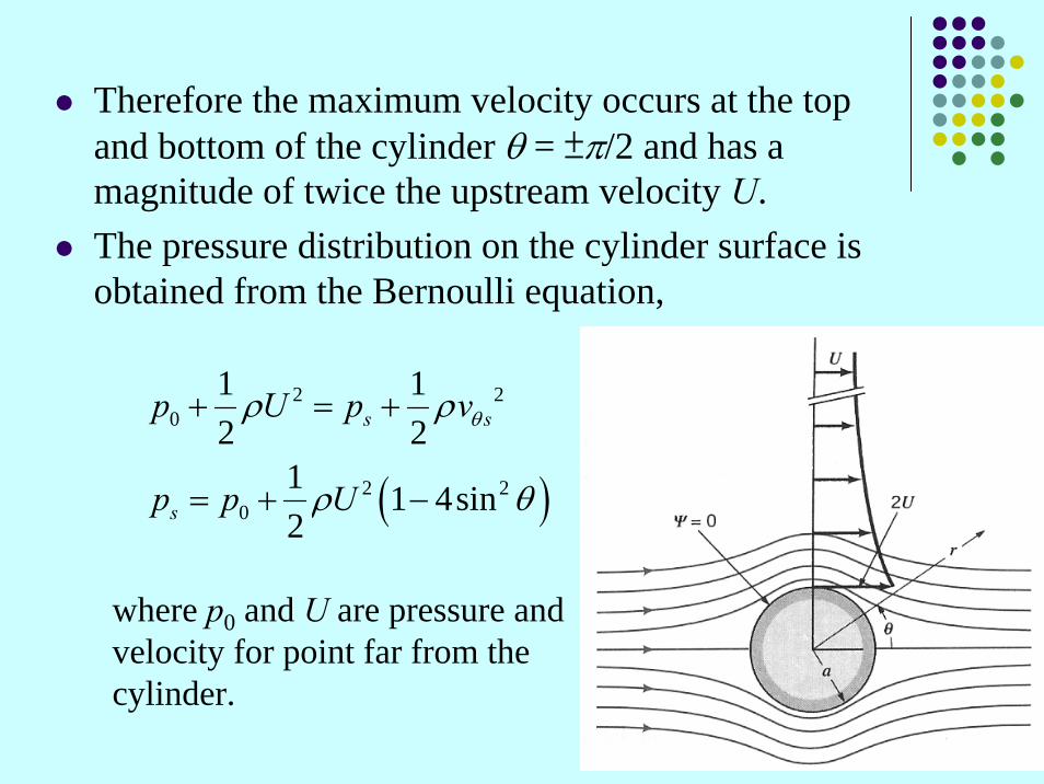
Therefore the maximum velocity occurs at the top and bottom of the cylinder θ = ±π/2 and has a magnitude of twice the upstream velocity U.The pressure distribution on the cylinder surface is obtained from the Bernoulli equation,
( )
2 20
2 20
1 12 2
1 1 4sin2
θρ ρ
ρ θ
+ = +
= + −
s s
s
p U p v
p p U
where p0 and U are pressure and velocity for point far from the cylinder.

The figure reveals that only on the upstream part of the cylinder is there approximate agreement between the potential flow and the experimental results.

The resulting force (per unit length) developed on the cylinder can be determined by integrating the pressure over the surface.
2
02
0
cos 0
sin 0
π
π
θ θ
θ θ
= − =
= − =
∫
∫
x s
y s
F p ad
F p ad
Both the drag and lift as predicted by potential theory for a fixed cylinder in a uniform stream are zero. since the pressure distribution is symmetrical around the cylinder.In reality, there is a significant drag developed on a cylinder when it is placed in a moving fluid. (d’Alembert paradox)
Ex 6.8 Potential flow--cylinder

By adding a free vortex to the stream function or velocity potential for the flow around a cylinder, then
where Γ is the circulationTangential velocity on the surface (r=a):
θπ
θφ
πθψ
2cos1
ln2
sin1
2
2
2
2
Γ+⎟⎟
⎠
⎞⎜⎜⎝
⎛+=
Γ−⎟⎟
⎠
⎞⎜⎜⎝
⎛−=
raUr
rraUr (6.119)
(6.120)
aU
rv
ars π
θψθ 2
sin2 Γ+−=
∂∂
−==
This type of flow could be approximately created by placing a rotating cylinder in a uniform stream. Because the presence of viscosity in any real fluid, the fluid in contact with the rotating cylinder would rotate with the same velocity as the cylinder, and the resulting flow field would resemble that developed by the combination of a uniform flow past a cylinder and a free vortex.
(6.121)

Location of the stagnation point
cylinder thefromaway located is 14/ if
surface on thelocation other someat is 14/1 if
or 0 0 if4
sin2
sin20
stag
stag
stag
stag
θπ
θπ
πθπ
θπ
θθ
→>Γ
→≤Γ≤−
=→=Γ
Γ=→
Γ+−==
Ua
Ua
UaaUv s

Force per unit length developed on the cylinder2
20
22 2
0 2 2 2
2
02 2
2
0 0
1 1 2 sin2 2 2
1 2 sin1 4sin2 4
cos 0
sin sin
s
s
x s
y s
p U p Ua
p p UaU a U
F p ad
UF p ad d U
π
π π
ρ ρ θπ
θρ θπ π
θ θ
ρθ θ θ θ ρπ
Γ⎛ ⎞+ = + − +⎜ ⎟⎝ ⎠
⎛ ⎞Γ Γ= + − + −⎜ ⎟
⎝ ⎠
= − =
Γ= − = − = − Γ
∫
∫ ∫For a cylinder with circulation, lift is developed equal to the product of the fluid density, the upstream velocity, and the circulation.
( )( ) +, counterclockwise the is downwardy
y
F U
U F
ρ= − Γ
+ Γ
The development of this lift on rotating bodies is called the Magnus effect.

6.7 Other Aspects of Potential Flow Analysis
Exact solutions based in potential theory will usually provide at best approximate solutions to real fluid problems.Potential theory will usually provide a reasonable approximationin those circumstances when we are dealing with a low viscosityfluid moving at a relatively high velocity, in regions of the flow field in which the flow is accelerating.Outside the boundary layer the velocity distribution and the pressure distribution are closely approximated by the potential flow solution.In situation when the flow is decelerating (in the rearward portion of the bluff body expanding region of a conduit), and adverse pressure gradient is reduced leading to flow separation, a phenomenon that are not accounted for by potential theory.
V6.10 Potential flow

PART CViscous Flow:
Navier-Stokes Equation(Sections 6.8-6.10)

6.8 Viscous FlowEquation of Motion
xx maF δδ = yy maF δδ = zz maF δδ =zyxm δδρδδ =
Thus
yxxx zxx
xy yy zyy
yzxz zzz
u u u ug u v wx y z t x y z
v v v vg u v wx y z t x y z
w w w wg u v wx y z t x y z
τσ τρ ρ
τ σ τρ ρ
ττ σρ ρ
∂ ⎛ ⎞∂ ∂ ∂ ∂ ∂ ∂+ + + = + + +⎜ ⎟∂ ∂ ∂ ∂ ∂ ∂ ∂⎝ ⎠
∂ ∂ ∂ ⎛ ⎞∂ ∂ ∂ ∂+ + + = + + +⎜ ⎟∂ ∂ ∂ ∂ ∂ ∂ ∂⎝ ⎠
∂ ⎛ ⎞∂ ∂ ∂ ∂ ∂ ∂+ + + = + + +⎜ ⎟∂ ∂ ∂ ∂ ∂ ∂ ∂⎝ ⎠

When a shear stress is applied on a fluid:• Fluids continuously deform (stress τ ~ rate of strain) • Solids deform or bend (stress τ ~ strain)
dydu
dtd =α
strain rate ~ velocity gradient
from Fox, McDonald and Pritchard, Introduction to Fluid Mechanics.
6.8.1 Stress-Deformation Relationships

6.8.1 Stress-Deformation RelationshipsFor incompressible Newtonian fluids it is known that the stresses are linearly related to the rate of deformation.
V1.6 Non-Newtonian behavior
,visc
visc, ,visc
,visc
2
2
2
yx x xz
xx xy xzy y yx z
ij yx yy yz
zx zy zz
yxz z z
vv v vvx y x x z
v v vv vy x y z y
vvv v vx z z y z
μ μ μ
σ τ ττ σ τ μ μ μτ τ σ
μ μ μ
⎡ ∂⎛ ⎞∂ ∂ ∂∂⎛ ⎞+ +⎢ ⎜ ⎟ ⎜ ⎟∂ ∂ ∂ ∂ ∂⎝ ⎠⎝ ⎠⎢⎡ ⎤ ⎢ ∂ ∂ ∂⎛ ⎞ ⎛ ⎞∂ ∂⎢ ⎥ ⎢≡ ≡ + +⎜ ⎟ ⎜ ⎟⎢ ⎥ ∂ ∂ ∂ ∂ ∂⎢ ⎝ ⎠ ⎝ ⎠⎢ ⎥ ⎢⎣ ⎦ ∂⎛ ⎞∂∂ ∂ ∂⎛ ⎞⎢ + +⎜ ⎟⎜ ⎟∂ ∂ ∂ ∂ ∂⎝ ⎠ ⎝ ⎠⎣
τ
⎤⎥⎥⎥⎥⎥⎥⎥
⎢ ⎥⎦
For incompressible, Newtonian fluids, the viscous stresses are:

xy yx
yz zy
zx xz
uy x
wz y
w ux z
υτ τ μ
υτ τ μ
τ τ μ
⎛ ⎞∂ ∂= = +⎜ ⎟∂ ∂⎝ ⎠
⎛ ⎞∂ ∂= = +⎜ ⎟∂ ∂⎝ ⎠
∂ ∂⎛ ⎞= = +⎜ ⎟∂ ∂⎝ ⎠
for normal stresses
2
2
2
xx
yy
zz
upx
pywpz
σ μ
υσ μ
σ μ
∂= − +
∂∂
= − +∂∂
= − +∂
for shearing stresses
( )13 xx yy zzp σ σ σ− = + +
But in normal stresses, there is additional contribution of pressure p, where
Can you figure out why the normal viscous stress σxx,visc can be expressed as ?2 u
xμ ∂∂
Consequently,
6.8.1 Stress-Deformation Relationships

For viscous fluids in motion the normal stresses are not necessarily the same in different directions, thus, the need to define the pressure as the average of the three normal stresses. Stress-strain relationship in cylindrical coordinate
2
12
2
rrr
r
zzz
pr
pr r
pz
θθθ
υσ μ
υ υσ μθ
υσ μ
∂= − +
∂∂⎛ ⎞= − + +⎜ ⎟∂⎝ ⎠
∂= − +
∂
1
1
rr r
zz z
r zrz zr
rr r r
z r
z r
θθ θ
θθ θ
υ υτ τ μθ
υ υτ τ μθ
υ υτ τ μ
⎛ ⎞∂∂ ⎛ ⎞= = +⎜ ⎟⎜ ⎟∂ ∂⎝ ⎠⎝ ⎠∂ ∂⎛ ⎞= = +⎜ ⎟∂ ∂⎝ ⎠∂ ∂⎛ ⎞= = +⎜ ⎟∂ ∂⎝ ⎠
Note: Notation x: plane perpendicular to x coordinatey: direction
xyτ
6.8.1 Stress-Deformation Relationships

6.8.2 The Navier-Stokes Equations
2 2 2
2 2 2
2 2 2
2 2 2
2 2 2
2 2 2
x
y
z
u u u u p u u uu w gt x y z x x y z
pu w gt x y z y x y z
w w w w p w w wu w gt x y z z x y z
ρ υ ρ μ
υ υ υ υ υ υ υρ υ ρ μ
ρ υ ρ μ
⎛ ⎞⎛ ⎞∂ ∂ ∂ ∂ ∂ ∂ ∂ ∂+ + + = − + + + +⎜ ⎟⎜ ⎟∂ ∂ ∂ ∂ ∂ ∂ ∂ ∂⎝ ⎠ ⎝ ⎠
⎛ ⎞⎛ ⎞∂ ∂ ∂ ∂ ∂ ∂ ∂ ∂+ + + = − + + + +⎜ ⎟⎜ ⎟∂ ∂ ∂ ∂ ∂ ∂ ∂ ∂⎝ ⎠ ⎝ ⎠
⎛ ⎞⎛ ⎞∂ ∂ ∂ ∂ ∂ ∂ ∂ ∂+ + + = − + + + +⎜⎜ ⎟∂ ∂ ∂ ∂ ∂ ∂ ∂ ∂⎝ ⎠ ⎝ ⎠
⎟
The Navier-Stokes equations are considered to be the governing differential equations of motion for incompressible Newtonian fluids

In terms of cylindrical coordinate2
2 2
2 2 2 2 2
2
2 2 2
1 1 2
1 1 1
r r r rr z
r r r rr
rr z
t r r r z
p g rr r r r r r r z
t r r r z
p g rr r r r r r
θ θ
θ
θ θ θ θ θ θ
θ θ θθ
υ υυ υ υ υρ υ υθ
υυ υ υ υρ μθ θ
υ υ υ υ υ υ υρ υ υθ
υ υ υρ μθ θ
⎛ ⎞∂ ∂ ∂ ∂+ + − +⎜ ⎟∂ ∂ ∂ ∂⎝ ⎠
⎛ ⎞∂∂ ∂ ∂∂ ∂ ⎛ ⎞= − + + − + − +⎜ ⎟⎜ ⎟∂ ∂ ∂ ∂ ∂ ∂⎝ ⎠⎝ ⎠∂ ∂ ∂ ∂⎛ ⎞+ + + +⎜ ⎟∂ ∂ ∂ ∂⎝ ⎠
∂ ∂∂ ∂ ⎛ ⎞= − + + − +⎜ ⎟∂ ∂ ∂ ∂⎝ ⎠
2
2 2
2 2
2 2 2
2
1 1
r
z z z zr z
z z zz
r z
t r r z
p g rz r r r r z
θ
θ
υυθ
υυ υ υ υρ υ υθ
υ υ υρ μθ
⎛ ⎞∂∂− +⎜ ⎟∂ ∂⎝ ⎠
∂ ∂ ∂ ∂⎛ ⎞+ + +⎜ ⎟∂ ∂ ∂ ∂⎝ ⎠⎛ ⎞∂ ∂ ∂∂ ∂ ⎛ ⎞= − + + + +⎜ ⎟⎜ ⎟∂ ∂ ∂ ∂ ∂⎝ ⎠⎝ ⎠
The Navier-Stokes Equations

6.9 Some Simple Solutions forViscous, Incompressible Fluids
There are no general analytical schemes for solving nonlinear partial differential equations, and each problem must be considered individually.
2 2 2
2 2 2
2 2 2
2 2 2
2 2 2
2 2 2
x
y
z
u u u u p u u uu w gt x y z x x y z
pu w gt x y z y x y z
w w w w p w w wu w gt x y z z x y z
ρ υ ρ μ
υ υ υ υ υ υ υρ υ ρ μ
ρ υ ρ μ
⎛ ⎞⎛ ⎞∂ ∂ ∂ ∂ ∂ ∂ ∂ ∂+ + + = − + + + +⎜ ⎟⎜ ⎟∂ ∂ ∂ ∂ ∂ ∂ ∂ ∂⎝ ⎠ ⎝ ⎠
⎛ ⎞⎛ ⎞∂ ∂ ∂ ∂ ∂ ∂ ∂ ∂+ + + = − + + + +⎜ ⎟⎜ ⎟∂ ∂ ∂ ∂ ∂ ∂ ∂ ∂⎝ ⎠ ⎝ ⎠
⎛ ⎞⎛ ⎞∂ ∂ ∂ ∂ ∂ ∂ ∂ ∂+ + + = − + + + +⎜⎜ ⎟∂ ∂ ∂ ∂ ∂ ∂ ∂ ∂⎝ ⎠ ⎝ ⎠
⎟
Nonlinear terms

6.9.1 Steady Laminar Flow BetweenFixed Parallel plates
0, 0wυ = =
Thus continuity indicates that
0ux
∂=
∂
for steady flow, ( )u u y=
0,x y zg g g and g o= = − =
2 2 2
2 2 2
2 2 2
2 2 2
2 2 2
2 2 2
x
y
z
u u u u p u u uu w gt x y z x x y z
pu w gt x y z y x y z
w w w w p w w wu w gt x y z z x y z
ρ υ ρ μ
υ υ υ υ υ υ υρ υ ρ μ
ρ υ ρ μ
⎛ ⎞⎛ ⎞∂ ∂ ∂ ∂ ∂ ∂ ∂ ∂+ + + = − + + + +⎜ ⎟⎜ ⎟∂ ∂ ∂ ∂ ∂ ∂ ∂ ∂⎝ ⎠ ⎝ ⎠
⎛ ⎞⎛ ⎞∂ ∂ ∂ ∂ ∂ ∂ ∂ ∂+ + + = − + + + +⎜ ⎟⎜ ⎟∂ ∂ ∂ ∂ ∂ ∂ ∂ ∂⎝ ⎠ ⎝ ⎠
⎛ ⎞⎛ ⎞∂ ∂ ∂ ∂ ∂ ∂ ∂ ∂+ + + = − + + + +⎜⎜ ⎟∂ ∂ ∂ ∂ ∂ ∂ ∂ ∂⎝ ⎠ ⎝ ⎠
⎟
maxu

Steady Laminar Flow Between Fixed Parallel platesThus
( )
2
2
1
2
2
1
21 2
0
0
0
1
1
12
p ux yp g p gy f xypz
d u pdy xdu p y Cdy x
pu y C y Cx
μ
ρ ρ
μ
μ
μ
∂ ∂= − +
∂ ∂∂
= − − → = − +∂∂
= −∂
∂=
∂
∂⎛ ⎞= +⎜ ⎟∂⎝ ⎠∂⎛ ⎞= + +⎜ ⎟∂⎝ ⎠
px
∂∂( is treated as a constant since it is not a function of y)
2 2 2
2 2 2
2 2 2
2 2 2
2 2 2
2 2 2
x
y
z
u u u u p u u uu w gt x y z x x y z
pu w gt x y z y x y z
w w w w p w w wu w gt x y z z x y z
ρ υ ρ μ
υ υ υ υ υ υ υρ υ ρ μ
ρ υ ρ μ
⎛ ⎞⎛ ⎞∂ ∂ ∂ ∂ ∂ ∂ ∂ ∂+ + + = − + + + +⎜ ⎟⎜ ⎟∂ ∂ ∂ ∂ ∂ ∂ ∂ ∂⎝ ⎠ ⎝ ⎠
⎛ ⎞⎛ ⎞∂ ∂ ∂ ∂ ∂ ∂ ∂ ∂+ + + = − + + + +⎜ ⎟⎜ ⎟∂ ∂ ∂ ∂ ∂ ∂ ∂ ∂⎝ ⎠ ⎝ ⎠
⎛ ⎞⎛ ⎞∂ ∂ ∂ ∂ ∂ ∂ ∂ ∂+ + + = − + + + +⎜⎜ ⎟∂ ∂ ∂ ∂ ∂ ∂ ∂ ∂⎝ ⎠ ⎝ ⎠
⎟

the constants are determined from the boundary conditions.
1
22
BCs : 0Thus 0
1 2
u for y hC
pC hxμ
= = ±=
∂⎛ ⎞= − ⎜ ⎟∂⎝ ⎠
Thus the velocity distribution becomes,
( )2 212
pu y hxμ
∂⎛ ⎞= −⎜ ⎟∂⎝ ⎠
which indicates that the velocity profile between the two fixed plates is parabolic.
Steady Laminar Flow Between Fixed Parallel plates
V6.11 No-slip boundary conditions
V6.13 Laminar flow

The volume rate of flow
( )2 2
32
3 33 3
3
12
12 3
12 3 3
23
h h
h h
h
h
pq u dy y h dyx
p yq h yx
p y hh hx
h px
μ
μ
μ
μ
− −
−
∂⎛ ⎞= = −⎜ ⎟∂⎝ ⎠⎡ ⎤∂⎢ ⎥= −
∂ ⎢ ⎥⎣ ⎦⎡ ⎤∂
= − + −⎢ ⎥∂ ⎣ ⎦∂
= −∂
∫ ∫
The pressure gradient is negative, since the pressure decreases in the direction of the flow.
Steady Laminar Flow Between Fixed Parallel plates

If Δp represents the pressure drop between two points a distance apart, thenl
3 3 22 2 , 3 3 2 3
p px
h p h p q h pq Vx hμ μ μ
Δ ∂= −
∂∂ Δ Δ
= − = = =∂
l
l l
Steady Laminar Flow Between Fixed Parallel plates
The maximum velocity umax , occurs midway y=0 between the two plates, thus
Vuxphu
23 or
2 max
2
max =∂∂
−=μ

The pressure field
The above analysis is valid for remains below about 1400
Problem 6.88: 10 tons on 8psi
( )
( )1 0
p gy f x
pf x x px
ρ= − +
∂⎛ ⎞= +⎜ ⎟∂⎝ ⎠where is a reference pressure at x=y=0
Thus the pressure variation throughout the fluid can be obtained from
0pp gy x px
ρ ∂⎛ ⎞= − + +⎜ ⎟∂⎝ ⎠ 2Re V hρμ
=
0p
Steady Laminar Flow Between Fixed Parallel plates

6.9.2 Couette FlowTherefore
21 2
12
pu y C y Cxμ
∂⎛ ⎞= + +⎜ ⎟∂⎝ ⎠
or in dimensionless form
The actual velocity profile will depend on the dimensionless parameter
This type of flow is called Couette flow.
boundary conditionsu=o at y=0, u=U at y=b
( )212
b pu U y byy xμ
∂⎛ ⎞= + −⎜ ⎟∂⎝ ⎠
2
12
u y b p y yU b U x b bμ
∂⎛ ⎞⎛ ⎞⎛ ⎞= − −⎜ ⎟⎜ ⎟⎜ ⎟∂⎝ ⎠⎝ ⎠⎝ ⎠
2
2b pP
U xμ∂⎛ ⎞= − ⎜ ⎟∂⎝ ⎠

Couette flowThe simplest type of Couette flow is one for which the pressure gradient is zero i.e. the fluid motion is caused by the fluid being dragged along by the moving boundary.
Thus
0px
yu Ub
∂=
∂
=
which indicates that the velocity varies linearly between the two plates.
e.g. : Journal bearingro-ri << ri
The flow in an unloaded journal bearing might be approximated by this simple Couette flow.

Example 6.9Example 6.9( )0 0
0
0 0
u w xy
p px z
x h p atmospheric pressuredp dpdx dz
υ υ υ∂= = = =
∂∂ ∂
= =∂ ∂= =
∴ = ∴ =
2
2
2
2
1
0 dgdx
ddxd x Cdx
υρ μ
υ γμ
υ γμ
= − +
=
= +
Therefore
on the film surface x=h, we assume that the shearing stress is zero
1
0xy xyd at x hdx
hC
υτ μ τ
γμ
⎛ ⎞= = =⎜ ⎟⎝ ⎠
= −

2nd integration2
2
0 2 0
20
200 0
3
0
20
2
2
3
h h
hx x C
x V C Vhx x V
hq dx x x V dx
hq V h
γ γυμ μ
υγ γυμ μ
γ γυμ μ
γμ
= − +
= = ∴ =
= − +
⎛ ⎞= = − +⎜ ⎟
⎝ ⎠
= −
∫ ∫
The average film velocity2
0 3q hV Vh
γμ
= = −
2
0 3hV γμ
>Only if , will there be a net upward flow of liquid.
Q: Do you find anything weird in this problem?

6.9.3 Steady, Laminar flow in Circular Tubes
Hagen–Poiseuille flow or Poiseuille flow steady, laminar flow through a straight circular tube of constant cross sectionConsider the flow through a horizontal circular tube of radius R
Assume the flow is parallel
( )
0
0
r
z
z z
v vvzv v r
θ= =∂
=∂
∴ =

Steady, Laminar flow in Circular Tubes
Thus
rpg
∂∂
−−= θρ sin0
θsinggr −=θ
θρ∂∂
−−=p
rg 1cos0
θθ cosgg −=
⎥⎦
⎤⎢⎣
⎡⎟⎠⎞
⎜⎝⎛
∂∂
∂∂
+∂∂
−=rvr
rrzp z10 μ
Integration of equations in the r and θ directions( )
( )1
1
sinp gr f z
gy f z
ρ θ
ρ
= − +
= − +
which indicate that the pressure is hydrostatically distributed at any particular cross section and the zcomponent of the pressure gradient, , is not a function of r or θ.
zp ∂∂ /

Steady, Laminar flow in Circular Tubesthe equation of motion in the z direction
Boundary conditions
21
21 2
1 1
12
1 ln4
z
z
z
v prr r r z
v pr r Cr z
pv r C r Cz
μ
μ
μ
∂∂ ∂⎛ ⎞ =⎜ ⎟∂ ∂ ∂⎝ ⎠∂ ∂⎛ ⎞= +⎜ ⎟∂ ∂⎝ ⎠
∂⎛ ⎞= + +⎜ ⎟∂⎝ ⎠
At r=0, vz is finite at the center of the tube, thus C1=0
At r=R, vz =0, then 22
14
pC Rzμ
∂⎛ ⎞= − ⎜ ⎟∂⎝ ⎠
Thus the velocity distribution becomes,
( )22
41 Rr
zpvz −⎟
⎠⎞
⎜⎝⎛
∂∂
=μ
That is, at any cross section, the velocity distribution is parabolic.

Steady, Laminar flow in Circular TubesVolume flow rate
zpRrdrRr
zprdrvQ
drrvdQRR
z
z
∂∂
−=−⎟⎠⎞
⎜⎝⎛
∂∂
==
=
∫∫ μπ
μππ
π
8)(
4122
)2(4
0
22
0
Let , thenzpp
∂∂
−=Δl lμ
π8
4 pRQ Δ= Poiseuille’s law
lμπ 8
2
2
PRRQV Δ
==
2 2
max 4 4R p R pv
zμ μ∂ Δ⎛ ⎞= =⎜ ⎟∂⎝ ⎠ l
so Vv 2max =
mean velocity
maximum velocity
the velocity distribution in terms of vmax2
max
1 ⎟⎠⎞
⎜⎝⎛−=
Rr
vvz

6.9.4 Steady, Axial, Laminar Flow in an Annulus
B.Cs:vz=0 at r=ro and r=ri
212 ln
41 CrCr
zpvz ++⎟
⎠⎞
⎜⎝⎛
∂∂
=μ
thus( ) ( )2 2
2 2 00 0
0
1 ln /4 ln /
iz i
i
r rpv r r r rz r rμ
⎡ ⎤−∂⎛ ⎞= − +⎢ ⎥⎜ ⎟∂⎝ ⎠ ⎢ ⎥⎣ ⎦
volume rate of flow
( )( )
( )( )
022 2
4 4
0
22 24 4
0
28 ln /
8 ln /
i
ro i
z o iir
o io i
i
r rpQ v rdr r rz r r
r rp r rr r
ππμ
πμ
⎡ ⎤−∂⎛ ⎞ ⎢ ⎥= = − − −⎜ ⎟ ⎢ ⎥∂⎝ ⎠⎣ ⎦
⎡ ⎤−Δ ⎢ ⎥= − − −⎢ ⎥⎣ ⎦
∫
l

The maximum velocity occur at the , mrr = 0zv r∂ ∂ =
( )
122 2
02ln /o i
mi
r rrr r
⎡ ⎤−= ⎢ ⎥
⎢ ⎥⎣ ⎦
The maximum velocity does not occur at the mid point of the annulus space, but rather it occurs nearer the inner cylinder.
To determine Reynolds number, it is common practice to use an effective diameter “hydraulic diameter” for on circular tubes.
μρ VD
R he =Thus the flow will remain laminar if remains below 2100.
perimeter wettedarea sctional-cross4×
=hD

6.10 Other Aspects of Differential Analysis
The solutions of the equations and not readily available.
VgpVVtV 2∇++−∇=⎟
⎟⎠
⎞⎜⎜⎝
⎛∇•+
∂∂ μρρ
0=•∇ V
6.10.1 Numerical MethodsFinite difference methodFinite element ( or finite volume ) methodBoundary element method
V6.15 CFD example
Recommended