________________________________________________________________________ Dick, Joseph M., and Dick, Matthew S. 2014. Developing an Analysis Process for Crime Hot Spot
Identification and Comparison. Volume 16, Papers in Resource Analysis. 15 pp. Saint Mary’s University of
Minnesota Central Services Press. Winona, MN. Retrieved (date) from http://www.gis.smumn.edu
Developing an Analysis Process for Crime Hot Spot Identification and Comparison
Joseph M. Dick and Matthew S. Dick
Department of Resource Analysis, Saint Mary’s University of Minnesota, Minneapolis, MN
55404
Keywords: Residential Burglary, GIS, Crime, Law Enforcement, Hot Spot, Kernel Density
Estimation, Prediction Accuracy Index, Global Statistical Tests
Abstract
This research focuses on using Geographic Information Systems (GIS) to identify crime hot
spots using kernel density estimation (KDE) pertaining to residential burglary. Global
statistical tests were applied prior to utilizing the KDE method to ensure valid, accurate
results and limit the influence of factors that may cause misinterpretation or error.
Considerations for parameter input into the KDE analysis were explored to enhance
consistency with statistical tests and output accuracy. Additionally, KDE outputs were tested
for predictive ability and compared with the prediction accuracy index (PAI). This process
can provide a foundation for predictive analysis to be utilized by law enforcement agencies to
develop crime prevention strategies.
Introduction
Law enforcement has a long history of
mapping crime locations and has been
performing crime analysis since their
establishment (Groff and La Vigne, 2001).
The utilization of GIS analysis plays an
important role in identifying crime hot
spots to predict future crimes for the
purpose of police intervention and
prevention (Groff and La Vigne).
This study focuses on developing a
spatial and temporal analysis process to
identify hot spots of crime and evaluate
the hot spots’ predictive capabilities
utilizing statistics. The aim of this study
was to produce statistically reliable crime
information for law enforcement
professionals to help develop strategies to
reduce and prevent crime. The process will
be applied to residential burglary crime
data obtained from the Saint Paul Police
Department (SPPD). The extent of the
study area included the Western District
police sector of the City of Saint Paul,
Minnesota.
Crime Hot Spots
Crime hot spots have become a popular
subject within the crime analyst discipline
but there is no established benchmark for
defining a hot spot (Harries, 1999). Eck,
Chainey, Cameron, Leitner, and Wilson
(2005) concur there is no widely accepted
definition, but offer a hot spot is “a place
that has many crimes.” A hot spot can be
described as an area that has a greater than
average number of crimes or risk of
victimization (Eck et al., 2005). Harries
offers that a hot spot is a type of clustering
within a spatial distribution, but not all
crime clusters can be defined as a hot spot
due to the characteristics unique to
different geographic areas.
Chainey, Reid, and Stuart (2002)
found global statistical tests can be applied
to a crime cluster to determine if it can be

2
established as a hot spot. Eck et al. (2005)
states it is advantageous to perform global
statistical tests for a better understanding
of the data, to visualize patterns within the
data before they are mapped, and to
support the validity of mapping outputs.
Crime Mapping Techniques
Chainey et al. (2002) suggests hot spot
maps provide easy interpretation of crime
occurrences, more precisely depicts spatial
distributions of crime and requires less
user input. According to Chainey,
Tompson, and Uhlig (2008), hot spot maps
typically use retrospective data for the
purpose of discovering high crime areas
requiring additional police resources to
address the crime problem. Chainey et al.
(2008) states a multitude of techniques for
hot spot mapping exist including point
mapping, thematic mapping, spatial
ellipses, grid thematic mapping, and kernel
density estimation (KDE).
The point mapping technique is a
wall pin crime map in digital format
displaying individual crime incidents (Eck
et al., 2005). It is best suited for displaying
small amounts of crime, but lacks the
functionality to interpret patterns or hot
spots (Chainey et al., 2002).
Thematic mapping incorporates
defined borders, such as political
boundaries, census tracts, or police beats,
with crime data (Eck et al., 2005). This
method allows for the quick interpretation
of information, displaying the intensity of
crime events for each border area within
the study area (Chainey et al., 2008). A
disadvantage of thematic mapping is the
potential for under or over-representation
of crimes that occur near or across the
boundaries within the study area (Eck et
al., 2005). Chainey et al. (2002) found the
modifiable areal unit problem applies as
another drawback to this technique.
Spatial ellipses are a technique
used to identify and group crime clusters
(Chainey et al., 2002). Ellipses are created
for each defined cluster of crime, and the
size and position of the ellipse is aligned
over the crime data points within the study
area. A benefit of this technique is not
being limited by boundaries, unlike
thematic mapping. Eck et al. (2005) states
spatial ellipses have multiple
disadvantages: 1) their shape does not
accurately represent the actual shape or
spatial distribution of clusters, 2)
parameter input by the user can greatly
affect the output, and 3) any data outside
the generated ellipses is not displayed,
leaving all other data irrelevant.
Grid thematic mapping is a process
of laying a uniform grid with a user-
specified cell size over a study area, and
each corresponding grid is shaded to
represent the level of crime events within
each cell (Chainey et al., 2008). Eck et al.
(2005) states this technique makes
identification of hot spots easier and is
more accurate than thematic mapping. Eck
et al. (2005) established that grid thematic
mapping is vulnerable to the modifiable
areal unit problem, and spatial detail is
diminished using the grid format, resulting
in a digitized or “blocky” map output
appearance.
The KDE method is widely
accepted as the most appropriate visual
crime data analytical technique (Chainey
et al., 2008). KDE creates a smooth
surface map output, not limited by shape
or boundary, continuously displaying the
variations of crime occurrences throughout
the study area (Williamson, McLafferty,
Goldsmith, McGuire, and Mollenkopf,
1998). The advantages of KDE include
readily identifiable crime clusters,
preservation of different crime densities
across the study area, and hot spot
locations and spatial distributions are more

3
precise (Eck et al., 2005). Williamson et
al., 1998 states KDE can additionally be
utilized for “quantitative comparisons over
time.” Tompson and Townsley (2009)
selected the KDE method in their spatial
and temporal study because of the level of
predictive accuracy it offered over all
tested hot spot methods. A drawback to
KDE is it can produce misleading map
outputs if the data is not statistically tested
to determine the proper input parameters
and the appropriate thematic range (Eck et
al., 2005).
Analysis Process
Global Statistical Tests
Global statistical tests for clustering and
standard distance are helpful in
determining patterns in crime data and can
promote a higher level of validity for
analysis results (Eck et al., 2005). Chainey
et al. (2002) developed a robust process
for creating statistically accurate hot spot
crime maps utilizing KDE analysis. The
process contains three separate tests: 1)
nearest neighbor test for clustering, 2)
standard distance test for dispersion, and
3) nearest neighbor test to determine a k-
value (Chainey et al., 2002).
The nearest neighbor test helps
create a more accurate mapping output
using geocoded point data for analysis
(Chainey et al., 2002). Eck et al. (2005)
offers that the nearest neighbor test for
clustering compares a distribution of data
with a sample that is randomly distributed.
Eck et al. (2005) states the test produces a
ratio of the average nearest neighbor
distance of the data against a randomly
distributed test sample. A test ratio number
substantially lower than one indicates that
clustering is present, near one indicates a
random distribution, and substantially over
one indicates a dispersed distribution
within the data tested according to Eck et
al.
The standard distance test relates to
the dispersion of crime data and should be
used to compare two different crime types
or the same crime type of different time
periods (Eck et al., 2005). Chainey et al.
(2002) states the resulting figure has a
direct correlation with the crime data
dispersion, a smaller figure indicates less
dispersion, a larger figure indicates more
dispersion.
The nearest neighbor test to
determine a bandwidth is used to set the
variable for how the smoothing analysis is
applied in the KDE tool (Williamson et
al., 1998). Williamson et al. (1998) states
the test measures the distance between
each data point and the user-specified
number of nearest neighbors and averages
them; resulting in a suggested bandwidth
value. The user-specified number of
nearest neighbors is referred to as the k-
value (Williamson et al., 1998). Selection
of the proper bandwidth ensures that the
smoothing performed during analysis nets
the most accurate result (Williamson et al.,
1998).
KDE Analysis
Chainey et al. (2002) states, “The kernel
density method creates a smooth surface
of the variation in the density of point
events across an area.” According to
Ratcliffe and McCullagh (1999), during
KDE analysis a grid is overlaid on the
study area with the user defining the cell
size within the grid. Next, a radius with its
size defined by the user is placed over
each cell weighting each point within the
kernel (Ratcliffe and McCullagh, 1999).
Finally, values for each grid cell are
calculated by summing the circle surfaces
for each location (Ratcliffe and
McCullagh, 1999).
4
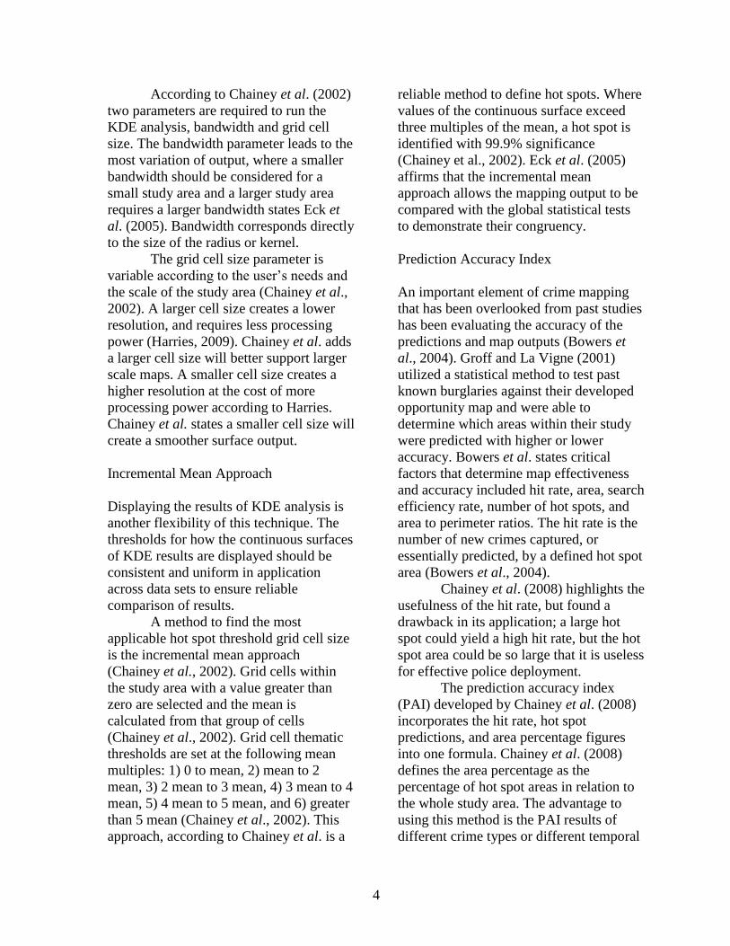
According to Chainey et al. (2002)
two parameters are required to run the
KDE analysis, bandwidth and grid cell
size. The bandwidth parameter leads to the
most variation of output, where a smaller
bandwidth should be considered for a
small study area and a larger study area
requires a larger bandwidth states Eck et
al. (2005). Bandwidth corresponds directly
to the size of the radius or kernel.
The grid cell size parameter is
variable according to the user’s needs and
the scale of the study area (Chainey et al.,
2002). A larger cell size creates a lower
resolution, and requires less processing
power (Harries, 2009). Chainey et al. adds
a larger cell size will better support larger
scale maps. A smaller cell size creates a
higher resolution at the cost of more
processing power according to Harries.
Chainey et al. states a smaller cell size will
create a smoother surface output.
Incremental Mean Approach
Displaying the results of KDE analysis is
another flexibility of this technique. The
thresholds for how the continuous surfaces
of KDE results are displayed should be
consistent and uniform in application
across data sets to ensure reliable
comparison of results.
A method to find the most
applicable hot spot threshold grid cell size
is the incremental mean approach
(Chainey et al., 2002). Grid cells within
the study area with a value greater than
zero are selected and the mean is
calculated from that group of cells
(Chainey et al., 2002). Grid cell thematic
thresholds are set at the following mean
multiples: 1) 0 to mean, 2) mean to 2
mean, 3) 2 mean to 3 mean, 4) 3 mean to 4
mean, 5) 4 mean to 5 mean, and 6) greater
than 5 mean (Chainey et al., 2002). This
approach, according to Chainey et al. is a
reliable method to define hot spots. Where
values of the continuous surface exceed
three multiples of the mean, a hot spot is
identified with 99.9% significance
(Chainey et al., 2002). Eck et al. (2005)
affirms that the incremental mean
approach allows the mapping output to be
compared with the global statistical tests
to demonstrate their congruency.
Prediction Accuracy Index
An important element of crime mapping
that has been overlooked from past studies
has been evaluating the accuracy of the
predictions and map outputs (Bowers et
al., 2004). Groff and La Vigne (2001)
utilized a statistical method to test past
known burglaries against their developed
opportunity map and were able to
determine which areas within their study
were predicted with higher or lower
accuracy. Bowers et al. states critical
factors that determine map effectiveness
and accuracy included hit rate, area, search
efficiency rate, number of hot spots, and
area to perimeter ratios. The hit rate is the
number of new crimes captured, or
essentially predicted, by a defined hot spot
area (Bowers et al., 2004).
Chainey et al. (2008) highlights the
usefulness of the hit rate, but found a
drawback in its application; a large hot
spot could yield a high hit rate, but the hot
spot area could be so large that it is useless
for effective police deployment.
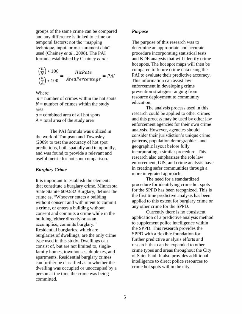
The prediction accuracy index
(PAI) developed by Chainey et al. (2008)
incorporates the hit rate, hot spot
predictions, and area percentage figures
into one formula. Chainey et al. (2008)
defines the area percentage as the
percentage of hot spot areas in relation to
the whole study area. The advantage to
using this method is the PAI results of
different crime types or different temporal
5
groups of the same crime can be compared
and any difference is linked to crime or
temporal factors; not the “mapping
technique, input, or measurement data”
used (Chainey et al., 2008). The PAI
formula established by Chainey et al.:
(𝑛𝑁) ∗ 100
(𝑎𝐴) ∗ 100
= 𝐻𝑖𝑡𝑅𝑎𝑡𝑒
𝐴𝑟𝑒𝑎𝑃𝑒𝑟𝑐𝑒𝑛𝑡𝑎𝑔𝑒= 𝑃𝐴𝐼
Where:
n = number of crimes within the hot spots
N = number of crimes within the study
area
a = combined area of all hot spots
A = total area of the study area
The PAI formula was utilized in
the work of Tompson and Townsley
(2009) to test the accuracy of hot spot
predictions, both spatially and temporally,
and was found to provide a relevant and
useful metric for hot spot comparison.
Burglary Crime
It is important to establish the elements
that constitute a burglary crime. Minnesota
State Statute 609.582 Burglary, defines the
crime as, “Whoever enters a building
without consent and with intent to commit
a crime, or enters a building without
consent and commits a crime while in the
building, either directly or as an
accomplice, commits burglary.”
Residential burglaries, which are
burglaries of dwellings, are the only crime
type used in this study. Dwellings can
consist of, but are not limited to, single-
family homes, townhouses, duplexes, and
apartments. Residential burglary crimes
can further be classified as to whether the
dwelling was occupied or unoccupied by a
person at the time the crime was being
committed.
Purpose
The purpose of this research was to
determine an appropriate and accurate
procedure incorporating statistical tests
and KDE analysis that will identify crime
hot spots. The hot spot maps will then be
compared to future crime data using the
PAI to evaluate their predictive accuracy.
This information can assist law
enforcement in developing crime
prevention strategies ranging from
resource deployment to community
education.
The analysis process used in this
research could be applied to other crimes
and this process may be used by other law
enforcement agencies for their own crime
analysis. However, agencies should
consider their jurisdiction’s unique crime
patterns, population demographics, and
geographic layout before fully
incorporating a similar procedure. This
research also emphasizes the role law
enforcement, GIS, and crime analysis have
in creating safer communities through a
more integrated approach.
The need for a standardized
procedure for identifying crime hot spots
for the SPPD has been recognized. This is
the first time predictive analysis has been
applied to this extent for burglary crime or
any other crime for the SPPD.
Currently there is no consistent
application of a predictive analysis method
to supplement police intelligence within
the SPPD. This research provides the
SPPD with a flexible foundation for
further predictive analysis efforts and
research that can be expanded to other
crime types and areas throughout the City
of Saint Paul. It also provides additional
intelligence to direct police resources to
crime hot spots within the city.

6
Data
Most raw data needed for this research
was collected from government agencies.
Two types of data were gathered, primary,
and supporting. The primary data obtained
were residential burglary crime data for
performing statistical, spatial, and
temporal analysis. Supporting data for the
development and production of base map
images were the second type of data
acquired.
Data Collection
Primary Data: Residential Burglary
Crimes
Primary data were obtained from the
SPPD Records Management System
(RMS). The SPPD RMS is a database
containing records of all calls for service,
documented police activity and written
incident reports for the SPPD. For each
incident entry in the SPPD RMS database,
many spatial and temporal attributes
accompany the incident as well as other
vital information about the incident. Only
specific data attributes were required for
each residential burglary crime incident
for this analysis.
Primary data were collected over a
five-year period, from January 2009
through December 2013. The SPPD RMS
has complete records of all reported
crimes within this five-year period. Pre-
2009 crime data contained in SPPD RMS
was incomplete and it is possible it could
have introduced an unknown amount of
error into the data set. The five-year period
also contains the most recent crime data
and was representative of current crime
incidents.
A query of the SPPD RMS
database was performed to acquire the
needed data (Figure 1). The data were
exported from the SPPD RMS database to
a Microsoft Excel spreadsheet.
Figure 1. Crime incident data attributes for analysis
derived from reported crime data originating from
the SPPD RMS database.
Primary Data Preparation
The queried data contained 5,307 entries.
Many duplicate entries were generated due
to multiple police reports written for the
same incident. Duplicate entries were
eliminated to prevent over-representation
of crime incidents and reduce analysis
error. The cleansed data totaled 3,311
incidents and were validated against the
SPPD RMS database count of 3,313
reported crimes during the five-year
period. This equaled an accuracy of
99.94%, ensuring the two missing crime
incidents would not significantly affect the
results of the study.
These crime data were then given
spatial reference for each data point by the
geocoding process. This was performed by
the SPPD to guarantee location accuracy
using a database containing only valid and
verified street addresses within the City of
Saint Paul. A shapefile containing all of
the geocoded residential burglary crime
•Residential Burglary
•Occupied and Unoccupied Dwelling
Reported Crime Data
•Within City of Saint Paul, Western District Police Sector 1
•Street Number
•Street Name
Spatial
Data
•From January 2009 through December 2013
•Month
•Day of Month
•Year
Temporal
Data

7
data was created. All of the data was
projected in UTM NAD83 Zone 15N.
The primary data was divided into
three prediction periods in preparation for
temporal analysis: 1) Entire data set, 2)
One-Year data sets, and 3) One-Month
data sets. In total, 66 separate data sets
were assigned to one of the three
prediction periods. Figure 2 describes the
data content for each prediction period.
Figure 2. Organization and content of the 66
residential burglary datasets into three prediction
periods for temporal analysis.
Supporting Data: Base Map Imagery
Supporting data for the development of a
base map displaying the Western District
police sector and its individual police grid
boundaries were collected. The Western
District borders and grid boundaries were
created using ESRI ArcMap and
ArcCatalog software referencing official
documents and data from the City of Saint
Paul and the SPPD (Figure 3).
Methods
This section describes processes
undertaken during analysis. Four main
stages of analysis were applied in this
research: 1) global statistical tests, 2) KDE
analysis, 3) incremental mean approach,
and 4) the development of the prediction
accuracy index. ESRI ArcMap and
ArcCatalog software were used for the
analysis.
Figure 3. The Western District study area within
the City of Saint Paul, Minnesota. District
boundary and grid lines are highlighted in dark
blue. The Western District is comprised of 88
police beat grids, and covers approximately 22.25
square miles.
Global Statistical Tests
All 66 residential burglary crime data sets
were subjected to three statistical tests
prior to running the KDE analysis. These
statistical tests provide optimal input
parameters for the analysis which increase
the hot spot accuracy and minimize output
error.
The nearest neighbor test for
clustering was performed on each data set
using the ArcGIS Average Nearest
Neighbor tool. The test provided a report
summary including the nearest neighbor
ratio and a z-score that serves as a
confidence indicator for the ratio (Figure
4). A z-score value of -1.65 or less
indicated that there was less than 10%
chance the distribution was random and
confirmed clustering was present within a
data set. Data sets without clustering were
not included in the KDE analysis.
•One data set
•Contains all data for 5-year time span
Entire Prediction
Period
•Five data sets
•Each data set contains data for a one year period
One-Year Prediction
Period
•60 data sets
•Each data set contains data for a one month period
One-Month Prediction
Period

8
Figure 4. Example of ArcGIS Average Nearest
Neighbor Tool summary report. Given the nearest
neighbor ratio of 0.689 and z-score of -5.61 for the
One-Month October, 2012 data set, there is less
than one percent likelihood that this clustered
pattern could be the result of random chance.
The standard distance test was
applied to each data set with the ArcGIS
Standard Distance tool using a circle size
of one standard deviation. This test
provides a way to test for dispersion and
allows for the comparison between the
data sets.
The nearest neighbor test to
determine bandwidth was performed on
each data set using the ArcGIS Calculate
Distance Band from Neighbor Count tool.
The 40 nearest neighbors were used for the
Entire data set, the nearest 20 neighbors
were used for the One-Year data sets, and
one nearest neighbor was used for
calculating the One-Month data sets. The
distances returned by this test were used as
the input for the bandwidth during the
KDE analysis for each data set.
KDE Analysis
The KDE analysis was performed on the
Entire, One-Year, and One-Month data
sets using the Kernel Density tool in
ArcGIS. Bandwidth was set using the
results from the ArcGIS Calculate
Distance Band from Neighbor Count tool.
A cell size of five meters was
chosen as this was the smallest cell size
possible that generated exceptional
smoothing accuracy and maintained a
reasonable processing time. The selected
parameters produced continuous surfaces
with variation in their densities according
to the input point crime data.
Incremental Mean Approach
The incremental mean approach was
applied to each KDE dataset to determine
the most accurate thresholds for viewing
analysis results and hot spot identification.
For each individual KDE raster dataset,
the mean value of all cells within the study
area were calculated, excluding all cells
with the value of zero.
The mean for the Entire data set
was calculated by itself as it was the only
data set within the prediction period and
the thematic thresholds were applied. To
ensure a consistent thematic threshold was
determined for the One-Year and One-
Month data sets, the mean of each KDE
raster was used to calculate an average
mean within its respective prediction
period. The average mean calculated for
each prediction period was then applied as
the basis for setting the thematic
thresholds. The calculated thematic
threshold values for all data sets are listed
in Table 1.
Predictive Accuracy Index
The PAI formula was applied to the data
sets where clustering of crime was present
as determined by the global statistical tests
and defined hot spot areas were identified

9
Table 1. Calculated thematic threshold values
(TTV) for Entire, One-Year, and One-Month data
sets generated from the incremental mean
approach. TTV in bold indicate hot spot areas of
99.9% significance. Mean
Multiples
Entire TTV One-Year
TTV
One-Month
TTV
0 to Mean 0.000058798 0.000011010 0.000003187
Mean to 2 Mean
0.000117596 0.00002202 0.000006374
2 Mean to
3 Mean
0.000176394 0.00003303 0.000009561
3 Mean to
4 Mean
0.000235192 0.00004404 0.000012748
4 Mean to
5 Mean
0.000293990 0.00005505 0.000015935
Greater
than 5
Mean
0.000293991 0.00005506 0.000015936
by the incremental mean approach. The
Entire data set, One-Year 2013 data set,
and One-Month December 2013 data set
were eliminated from analysis as there
were no future crime data for comparison
to these data sets.
PAI was calculated for the One-
Year data sets using future crime data
from the following year. For example, to
test the predictive ability of the One-Year
2009 hot spot data, the 2010 residential
burglary point data was used. Points
landing within the hot spot areas were
assumed to be predicted by the hot spots.
One-Month data sets had two
comparison processes applying PAI. First,
for a given One-Month data set, accuracy
was tested by the future crime data from
the following month. For example, the
predictive ability of the One-Month
August 2010 hot spot data was tested
using September 2010 residential burglary
point data (Figure 5). Points landing
within the hot spot areas were assumed to
be predicted by the hot spots.
Second, for a given One-Month
data set, accuracy was tested by the same
month of the following year. For example,
the One-Month August 2010 hot spot data
Figure 5. Hot spot area map for One-Month August
2010 Month to Next Month comparison with
September 2010 residential burglary point data
displayed.
was tested using the August 2011
residential burglary point data (Figure 6).
Points landing within the hot spot areas
were assumed to be predicted by the hot
spots.
Results
The KDE analysis produced hot spot areas
of statistical significance in data sets
where clustering was present. Applying
the PAI to the hot spot areas provided
further comparison of the results.
Residential burglary crime trends can be
recognized in certain areas of the Western
District over the Entire, One-Year, and
One-Month data sets.
Entire Data Set
KDE analysis of the Entire data set

10
Figure 6. Hot spot map for One-Month August
2010 Month to Same Month Next Year comparison
with August 2011 residential burglary point data
displayed.
produced hot spots in 17 of 88 grids of the
Western District (Figure 7). Hot spots
were generally located in the eastern and
north central areas of the Western District.
The Entire data set was not subjected to
PAI as there was no future crime data to
apply to this data set.
One-Year Data Sets
KDE analysis of the One-Year data sets
produced hot spots in 27 of 88 grids of the
Western District (Figure 8). The hot spots
were generally located in the eastern and
north central areas of the Western District,
comparable with the Entire data set.
PAI analysis was applied to the
One-Year data sets 2009 through 2012
(Table 2). The One-Year 2013 data set
was excluded from PAI analysis, as there
were no future crime data to apply to this
data set. PAI values for 2009 through 2012
Figure 7. Hot spot map for Entire data set showing
hot spot areas within the Western District.
Figure 8. Hot spot map for One-Year data sets
2009 through 2012. The color of the hot spot
corresponds to the year of data set it represents.
were consistent as the range between

11
values was 0.99.
Table 2. PAI statistics for One-Year data sets 2009
through 2012.
One-Year
Data Sets
PAI Value
2009 3.53
2010 3.66
2011 3.16
2012 4.15
Mean 3.63
The One-Year 2012 data set
achieved the highest PAI value of 4.15.
The One-Year 2012 data set hot spots
predicted 118 of the 609 residential
burglary crimes of 2013.
The One-Year 2011 data set
achieved the lowest PAI value of 3.16.
The One-Year 2011 data set hot spots
predicted 171 of the 710 residential
burglary crimes of 2012.
One-Month Data Sets
KDE analysis of the One-Month data sets
produced a wider variety of hot spot
locations within the Western District
compared to the Entire and One-Year data
sets. The size of the hot spots for One-
Month data sets were generally smaller in
area than those of the Entire and One-Year
Data sets, more dispersed, and were
greater in number.
PAI analysis was applied to the
month to next month comparison (Table
3). The PAI values for each data set in this
comparison are listed in Figure 9. The
average PAI value from the 42 One-Month
data sets was 3.92. Ten One-Month data
sets did not predict any next month
residential burglary crimes and resulted in
a PAI value of zero. The July 2012 One-
Month data set produced the highest PAI
value of 26.06.
PAI analysis was applied to the
month to same month next year
comparison (Table 3). The PAI values for
each data set in this comparison are shown
in Figure 10. The average PAI value from
the 42 One-Month data sets was 2.44. Ten
One-Month data sets did not predict any
same month next year residential burglary
crimes and resulted in a PAI value of zero.
The April 2012 One-Month data set
produced the highest PAI value of 12.50.
Table 3. PAI statistics for One-Month data sets
Month to Next Month and Month to Same Month
Next Year comparisons.
Month to
Next Month
PAI Value
Month to
Same
Month Next
Year
PAI Value
Mean 3.92 2.44
Std. Deviation 3.44 1.58
Minimum 0 0
Maximum 26.06 12.50
Discussion
The purpose of this study was to find an
accurate method to produce hot spot maps
using KDE analysis and compare the
accuracy of the results. A secondary
purpose was to bring the methodology to
the SPPD as a tool to be used for decision-
making for reducing and preventing crime.
Hot Spots
Hot spots produced by this study were
consistently located in the same areas
throughout the Entire, One-Year, and One-
Month data sets although the size of the
hot spots varied. This is an indication that
the hot spots have identified long-term
crime trends that have been occurring in
the Western District throughout the five
years of data that were analyzed. This
insight could be used by law enforcement
to develop a strategy to address residential
burglaries in these problem areas.
The Entire and One-Year hot spots

12
differ from the One-Month hot spots as
they are more appropriate for identifying
long-term crime trends. Information on
long-term crime trends would be useful for
administrative personnel to develop a
strategy to combat areas that are
consistently plagued with crime.
The One-Month hot spot areas
tended to be smaller in size and focused on
neighborhoods rather than entire grids of
the Western District. One-Month hot spots
located pockets of crime throughout the
Western District outside areas identified
by the Entire and One-Year hot spots. This
is an indication the One-Month prediction
period has the ability to identify short-term
crime trends that are not significant
enough to be displayed as a hot spot by the
Entire and One-Year data sets. The
information produced by One-Month hot
spots would be useful for patrol personnel
for day-to-day operations at the street
level.
PAI Value Comparisons
The PAI values for each of the One-Year
data sets were similar, inferring areas with
consistently high densities of burglaries
were identified by the hot spots. This also
suggests the One-Year prediction period is
a reliable temporal measure for the data
and study area for this research. The
consistency between the results of One-
Year data sets can be attributed to the
larger amount of data they contain versus
the smaller One-Month data sets.
In contrast, the PAI values for the
month to next month comparison were
more inconsistent, ranging from zero to
26.06. PAI values for the same month to
next year comparison were similarly
inconsistent, ranging from zero to 12.50.
This may be due to the One-Month data
sets identifying short-term crime trends
that change more rapidly than long-term
trends.
The month to next month
comparison PAI values in general appear
to be higher than the month to same month
next year comparison (Figures 9 and 10).
This observation was statistically tested
with the t-test for equality of means
assuming equal variance. Data for the
years 2009 through 2012 were used in the
t-test for both comparisons. The t-test did
not show a statistically significant
difference between the mean PAI values
for the two comparisons (Table 4).
Figure 9. Actual PAI values for One-Month prediction period Month to Next Month comparison.
0
5
10
15
20
25
30
Jan Feb Mar Apr May Jun Jul Aug Sep Oct Nov Dec
One-Month Prediction Period PAI Values
Month to Next Month Comparison
2009
2010
2011
2012
2013

13
Figure 10. Actual PAI values for One-Month prediction period Month to Same Month Next Year comparison
Table 4. Results of t-test for equality of means of the
One-Month prediction period comparisons.
Levene's Test for Equality of Variances
F 2.076
Sig. 0.155
t-test for Equality of Means
T 1.822
Df 64
Sig. (2-tailed) 0.073
Mean Difference 1.889
Std. Error Difference 1.037
95% Confidence Interval
of the Difference
Lower:
-0.182
Upper:
3.960
Sources of Error
Determining a K-Value
One of the advantages of KDE analysis is
the amount of flexibility the user has in
setting the parameters affecting the output
results. This has the potential to introduce
error into results and create inconsistent
results that cannot be used for accurate
comparison.
For example, determining an
appropriate k-value is an important step for
KDE analysis due to its large influence on
the results. Initially, a k-value of 20 was
applied to all data sets in this study as
suggested by Chainey et al. (2002). The k-
value worked well for the One-Year data set,
but not for the Entire and One-Month data
sets. The suggested k-value produced a
result that was too small in area for the
Entire data set and too large in area for the
One-Month data sets. Appropriate k-values
for each prediction period were determined
utilizing the research of Williamson et al.
(1998), finding larger data sets require a
larger k-value and smaller data sets require a
smaller k-value. A k-value of 40 for the
Entire data set and one for the One-Month
data sets produced acceptable results. This
troubleshooting process highlights the need
for the user to make adjustments to
parameters based on their unique study area
and data set.
Unreported Crime
It is recognized that crimes go unreported.
This research does not account for any
unreported crimes. There is no known
method for accurately determining the
amount of unreported crime. However, the
actual number of residential burglary crimes
within the Western District from 2009 to
2013 has the potential to be higher than the
number of crimes accounted for in the data
set used in this research. It is also unknown
what impact, if any, unreported crime would
have on the results of this study.
0
5
10
15
20
25
30
Jan Feb Mar Apr May Jun Jul Aug Sep Oct Nov Dec
One-Month Prediction Period PAI Values
Month to Same Month Next Year Comparison
2009
2010
2011
2012

14
Future Directions
The KDE analysis method used for this
research could be expanded to include other
crime types. Results from this research
could benefit from being compared to other
crime types in order to determine if other
crimes are more or less effectively predicted
by this analysis method. Further temporal
analysis could prove useful. Analyzing the
data by day of week, week of the year, or
seasons of the year could provide additional
insight on crime trends (Figures 11 and 12).
An additional expansion of this
research could be the creation of a crime
awareness and alert system for the residents
of the Western District. For example, when
a crime hot spot is identified within a grid of
the Western District, residents within that
grid would be notified of the increase of
criminal activity in the neighborhood. This
would demonstrate that law enforcement is
making a proactive effort to address
communities that experience elevated levels
of crime.
Conclusion
This study was able to accurately identify
Figure 11. Number of residential burglaries by day of
week from 2009 through 2013 within the Western
District. Day of week temporal analysis could
provide additional insight into crime patterns and
trends
hot spots of crime within the study area by
applying global statistical tests to the data
prior to performing the KDE analysis
method. The results provide an easily
interpreted visual representation of where
high numbers of burglaries occurred.
Application of the PAI allows for the hot
spot results to be tested for their predictive
ability further enhancing the potential for the
results to aid in reducing or preventing
crime. The process can serve as a foundation
for predictive analysis and can be expanded
to further spatial and temporal analysis for
Figure 12. Number of residential burglaries over time by month from 2009 through 2013 within the Western
District. Seasonal temporal analysis could identify unique crime trends or patterns.
050
100150200250300350400450500550600
Sun Mon Tue Wed Thu Fri Sat
0
10
20
30
40
50
60
70
80
90
100
JAN
20
09
MA
R
MA
Y
JUL
SE
P
NO
V
JAN
20
10
MA
R
MA
Y
JUL
SE
P
NO
V
JAN
20
11
MA
R
MA
Y
JUL
SE
P
NO
V
JAN
20
12
MA
R
MA
Y
JUL
SE
P
NO
V
JAN
20
13
MA
R
MA
Y
JUL
SE
P
NO
V

15
other crime types by law enforcement
agencies.
Acknowledgements
The authors would like to thank the RA staff
at Saint Mary’s University, specifically, Mr.
John Ebert, Dr. Dave McConville, and Ms.
Greta Bernatz. We want to thank our family
for their support, guidance, and
encouragement during our graduate studies.
Lastly, we recognize the Saint Paul Police
Department for providing crime data for this
study.
References
Bowers, K. J., Johnson, S. D., and Pease, K.
2004. Prospective Hot-Spotting The Future
of Crime Mapping?. British Journal of
Criminology, 44(5), 641-658. DOI:
10.1093/bjc/azh036.
Chainey, S., Reid, S., and Stuart, N.
2002. When is a Hotspot a Hotspot? A
Procedure for Creating Statistically Robust
Hotspot Maps of Crime. In D. Kidner, G.
Higgs, and S. White (Eds.), Socio-
Economic Applications of Geographic
Information Science, (pp. 21-36). London,
England: Taylor and Francis.
Chainey, S., Tompson, L., and Uhlig, S.
2008. The Utility of Hotspot Mapping for
Predicting Spatial Patterns of
Crime. Security Journal, 21(1), 4-28.
Eck, J. E., Chainey, S., Cameron, J. G.,
Leitner, M., and Wilson, R. E. 2005.
Mapping Crime: Understanding Hot Spots.
U.S. Department of Justice, Office of
Justice Programs, National Institute of
Justice. 1-79. National Criminal Justice
Reference Service Publication No. NCJ
209393.
Groff, E. R., and La Vigne, N. G. 2001.
Mapping an Opportunity Surface of
Residential Burglary. Journal of Research
in Crime and Delinquency, 38(3), 257-278.
DOI: 10.1177/0022427801038003003.
Harries, K. 1999. Mapping Crime: Principal
and Practice. U.S. Department of Justice,
Office of Justice Programs, National
Institute of Justice. 1-206. National
Criminal Justice Reference Service
Publication No. NCJ 178919.
Johnson, S. D., and Bowers, K. J. 2004. The
Burglary as Clue to the Future, The
Beginnings of Prospective Hot-
Spotting. European Journal of
Criminology, 1(2), 237-255. DOI:
10.1177/1477370804041252.
Ratcliffe, J. H., and McCullagh, M. J. 1999.
Hotbeds of Crime and the Search for
Spatial Accuracy. Journal of Geographical
Systems, 1(4), 385-398. DOI:
10.1007/s101090050020.
Tompson, L., and Townsley, M. 2009.
(Looking) Back to the Future: Using
Space-Time Patterns to Better Predict the
Location of Street Crime. International
Journal of Police Science &
Management, 12(1), 23-40. DOI:
10.1350/ijps.2010.12.1.148.
Williamson, D., McLafferty, S., Goldsmith,
V., McGuire, P., and Mollenkopf, J. 1998.
Smoothing Crime Incident Data: New
Methods for Determining Bandwidth in
Kernel Estimation. Paper presented at
18th ESRI International User Conference,
San Diego, July 27-31. Retrieved March 8,
2014 from http://proceedings.esri.com/
library/userconf/proc98/PROCEED/TO850
/PAP829/P829.HTM.
Recommended