
Page i
Determination of Residual Stresses in a Carbon-Fibre Reinforced Polymer using the
Incremental Hole-Drilling Technique
Author: Smart K Okai
(Student number: 384029)
School of Mechanical, Industrial and Aeronautical Engineering
University of the Witwatersrand,
Johannesburg, South Africa
Supervisor: Professor J.P Nobre
A Research Report submitted to the Faculty of Engineering and the Built Environment,
University of the Witwatersrand, in fulfillment of the requirements for the degree of Master of
Science in Engineering(Mechanical Engineering)
SUBMITTED ON 30TH
JANUARY, 2017

Page i
DECLARATION
I hereby declare that I am aware that plagiarism (the use of some else’s work without their
permission and/or without acknowledging the original source) is wrong. I confirm that the work
submitted for assessment for the above degree is my own unaided work except where I have
explicitly indicated otherwise. It has not been submitted before for any degree or examination at
any other University.
Signed this ………day of ………….2017
_________________________________
Smart Koranteng Okai
Certified by My Supervisor:
Professor J.P. Nobre
______________________ Date______________

Page ii
DEDICATION
This research project is dedicated to my uncle Mr Seth Kwasi Yeboah for his selfless pieces of
advice and encouragement given to me towards the completion of this work. Again it is also
dedicated to all best wishers and friends.

Page iii
ACKNOWLEDGEMENT
Ebenezer, this is how far the lord has brought me. May his name be praised and glorified.
I would like to express my profound gratitude to the almighty God for the strength and power given
to me to undertake this research work. I am thankful to all those who in one way or the other
contributed in the successful completion of this work.
My heartfelt gratitude goes to my supervisor Professor João-Paulo Nobre for his ever willingness to
assist; give directions, offer suggestions and pieces of advice, and sharing of knowledge to make
this project a success.

Page iv
ABSTRACT
An extensive variety of experimental techniques exist to determining residual stresses, but few of
these techniques is suitable, however, for finding the residual stresses that exist in orthotropic or
anisotropic layered materials, such as carbon-fibre reinforced polymers (CFRP). Among these
techniques, particularly among the relaxation techniques, the incremental hole-drilling technique
(IHD) has shown to be a suitable technique to be developed for this purpose. This technique was
standardized for the case of linear elastic isotropic materials, such as the metallic alloys in general.
However, its reliable application to anisotropic and layered materials, such as CFRP materials,
needs to be better studied. In particular, accurate calculation methods to determine the residual
stresses in these materials based on the measured in-depth strain relaxation curves need to be
developed.
In this work, existing calculation methods and already proposed theoretical approaches to determine
residual stresses in composite laminates by the incremental hole-drilling technique are reviewed.
The selected residual stress calculation method is implemented using MATLAB. For these
calculations, specific calibration coefficients have to be numerically determined by the finite
element method, using the ANSYS software. The developed MATLAB scripts are then validated
using an experimental procedure previously developed. This experimental procedure was performed
using CFRP specimens, with the stacking sequence [0o, 90
o]5s and, therefore, this composite
laminate was selected as case study in this work.
Some discrepancies between the calculated stresses using the MATLAB scripts and those imposed
during the experimental calibration procedure are observed. The errors found could be explained
considering the limitations inherent to the incremental hole-drilling technique and the theoretical
approach followed. However, the obtained results showed that the incremental hole-drilling can be
considered a promising technique for residual stress measurement in composite laminates.
Keywords: residual stress, carbon fibre reinforced polymer, incremental hold drilling technique.

Page v
TABLE OF CONTENTS
TITLE PAGE
DECLARATION……………….……………………………………………………………….........i
DEDICATION ..................................................................................................................................ii
ACKNOWLEDGEMENT………………………………………………………………………......iii
ABSTRACT…………………………………………………………………………………....……iv
TABLE OF CONTENT………………………………………………………………………….......v
LIST OF FIGURES………………………………………………………………………………..viii
LIST OF TABLES…………………………………………………………………………………...x
NOMENCLATURE……………………………………………………………………………........xi
1. INTRODUCTION….......................................................................................................................1
1.1 Purpose of the research…………………………………………………………………..........2
1.2 Research motivation……………………………………………………………………..........2
1.3 Problem statement……………………………………………………………………….........3
2. LITERATURE REVIEW………………… ……………………….……………………..……3
2.1 Introduction……………………………………………………………………………...........3
2.2 Fibre reinforced polymers………………………....................................................................4
2.3 Carbon fibre reinforced polymers (CFRP)………………………………….....………..........5
2.4 Classification and types of carbon fibres ……………………………………………….........6
2.5 Isotropic materials and anisotropic materials……………………….………...………….......7
2.6 Available techniques for residual stress determination in CFRP……...…………….……….8
2.6.1 First ply failure………..................................................................................................9
2.6.2 Hole-drilling technique………………………………...………………………….......9
2.6.3 Ring Core method……………………………………………..……………………...12
2.6.4 The slitting method or Crack compliance method……………………..……............12
2.6.5 Layer removal Method…………………………………………..…………………...13
2.6.6 Deep hole method…………………………………...……………………………….13
2.6.7 Sachs Method……………………………………………………….….....................14

Page vi
2.7 The incremental hole-drilling technique and its application to composite laminates………15
2.7.1 Introduction…………………………………………………………………………..15
2.7.2 Strain gauge rosettes.……………………………………………………………........17
2.7.3 Residual stress evaluation procedures for orthotropic/anisotropic layered material..18
3. RESEARCH AIMS AND OBJECTIVES……………………………………………….….......23
4. RESEARCH AIMS AND OBJECTIVES……………………………………………………....23
5. RESEARCH METHODS…….…………………………………………………………...........24
5.1 Numerical procedure………………………………..………………….………….…..….24
5.1.1 Introduction……………………………………………..……………………….…..….24
5.1.2 Determination of Calibration coefficients……………………………………………....25
5.2 Materials and experimental procedure………………………………………………........26
5.2.1 Material and specimens…..……………………………………………………………...26
5.2.2 Brief description of the experimental procedure used for validation purposes………....27
5.2.3 Incremental hole-drilling parameters…………………………………………………....30
6. MATLAB SCRIPT DEVELOPMENT….………………………………………………….…...31
7. RESULTS AND DISCUSSION………………………………………………………………...34
7.1 Calibration coefficient matrices............................................................................................34
7.2 Experimental in-depth strain relaxation distribution……………………………………….42
7.3 Calculated stress distribution and validation of the MATLAB scripts developed…………44
7.3.1 Effect of the drill bit geometry…………………………………………………………..46
7.3.2 Effect of the numerical uncertainties……………………………………………………47
7.3.3 Thermo-mechanical effects of the cutting procedure…………………………………...48
7.3.4 Limitation of the theoretical approach used for residual stress calculation…………….48
8. CONCLUTION…………………………………………………………………………………49

Page vii
9. REFERENCES…………………………………………………………………………...........51
10. APPENDIX……………………………………………………………………………..........55

Page viii
LIST OF FIGURES
Figure 2.1: Carbon fibre reinforced composite……………………………………………….......5
Figure 2.2: composite materials constituents. [13]………………………………………………..5
Figure 2.3: Relative locations of the hole and the strain (figure from [21])…………………….11
Figure 2.4: schematic diagram of the slitting method…………………………………………...13
Figure 2.5: a schematic diagram of the Sachs Method………………………………………......15
Figure 2.6: Incremental hole-drilling technique instruments use for the determination
of residual stresses in carbon fibre reinforced polymer: SINT MTS3000
(left) and Vishay MS200 milling guide (right)..........................................................17
Figure 2.7: Three strain gauges rosettes existing in the ASTM E837-13 [33]………………….18
Figure 2.8: Strain gauge rosette arrangements placed around where the hole was to be
drilled for determining residual stress[41]……………………………………....…..20
Figure 5.1: Finite element models after the first increment [3]………………………………….25
Figure 5.2: Fifth drilling stage…………………………………………………………………....26
Figure 5.3: Superposition principle to eliminate the initial residual stresses……………….…...28
Figure 5.4: Sequence of applied load cycles during the calibration procedure ………………...29
Figure 5.5: The coordinate system, the hole geometry and the position three-clockwise (CW)
strain gauge rosette for the incremental hole-drilling method [25]…………………31
Figure 7.1: 3D finite element mesh used in the FEM simulation of the [0/90]5s composite
laminate………………………………………………………………………………...35
Figure 7.2: 3D finite element mesh used in the hole-drilling FEM simulation of the
[0/90]5s composite laminate (closer view) – two depth increments per ply
were used……………………………………………………………………………..35
Figure 7.3: Relative size of the strain gauge area in the 3D finite element mesh used in the
hole- drilling FEM simulation of the [0/90]5s composite laminate
(1mm hole-depth)……………………………………………………………………...36
Figure 7.4: von Mises stress field (left) and strain field during the determination of the
coefficient constants matrix Ain (1mm hole-depth)……………………………….....37
Figure 7.5: Strain relaxation against depth increment generated using MATLAB code………...43
Figure 7.6: Minimum principal stresses and maximum principal stresses calculated by the
MATLAB scripts developed ………………………………………………………….44

Page ix
Figure 7.7: Observed error [] between the maximum principal stress calculated by the
MATLAB scripts developed and the expected stress value………………………..46
Figure 7.8: Micrograph of a drilled hole showing the remaining portion which was not
removed [45] …………………………………………………………………………41
Figure 7.9: Angular variation of relieved strain in materials of varying
degree of axial orthotropy. ASTM strain gauge geometry. [33]……………………44

Page x
LIST OF TABLES
Table 5.1 Properties of the material used in the test [43]……………………………………..….27
Table 5.2 incremental hole-drilling parameters previously used during the tests [32, 43]………..30
Table 7.1 – Calibration coefficient matrix Ain……………………………….……………….......39
Table 7.2– Calibration coefficient matrix Bin……………………………………….………….....40
Table 7.3 – Calibration coefficient matrix Cin…………………………………………………….41
Table 7.4 Strain-depth relaxation values obtained during the experimental calibration [40]……..42
Page xi
NOMENCLATURE
Symbols/abbreviations Descriptions Unit
ASTM American Society of Testing and Materials
CFRP Carbon fibre reinforced polymer -
FEM Finite Element Method
PMC Polymer Matrix Composite -
IHDT Incremental hole drilling technique -
IHD Incremental hole drilling -
HDM Hole drilling method -
UHM Ultra-high-modulus
PAN polyacrylonitrile
HM High-modulus, type HM
IM Intermediate-modulus, type
HT High-Tensile,
SHT Super high-tensile
IHT Intermediate-heat-treatment
MPa Mega Pascal MPa
GPa Giga Pascal GPa
Longitudinal stress MPa
Transverse stress MPa
Calibration Constant
Calibration Constant
Calibration Constant
FEA Finite element analysis
EL Elastic limit in the longitudinal direction
ET Elastic limit in the transverse direction

Page 1
1. INTRODUCTION
Carbon Fibre Reinforced Polymer (CFRP) is a Polymer Matrix Composite (PMC) material reinforced
by carbon fibers. The carbon fibres possess the highest specific mechanical properties such as
modulus of elasticity and strength. Because CFRP are characterized by the following mechanical
properties: light in weight, high strength to weight ratio, very high modulus of elasticity to weight
ratio, high fatigue strength, good corrosion resistance, very low coefficient of thermal expansion and
low impact resistance, they are perfect choice for a large number of structural applications, ranging
from aircraft, helicopters and spacecraft through to boats, ships and offshore platforms and to
automobiles, sports goods, chemical processing equipment and civil infrastructure such as bridges
and buildings.
Residual stresses are normally stresses that build up or remain in equilibrium in a solid material
without the application of external loads. They can be found in most composite laminates. During
manufacturing or operation of the composite structure, residual stresses can be developed in either
process, due to different coefficients of thermal expansion of matrix and fibres or the curing process.
Since residual stresses can be a large magnitude they may affect the strength of composite structures
and their external load bearing capacity [1].
Notwithstanding how they are formed, residual stresses in carbon fibre reinforced polymer (CFRP)
adversely impact on the mechanical performance of composites and it is necessary to develop
techniques to characterize them before these materials are placed in service. Residual stresses can
cause failure of a part below the design load or, under fatigue loading, when neglected during design,
prior to the useful design life of the part [2, 3].
There are a lot of techniques which are used to determine residual stresses in composite materials.
Generally, the experimental techniques used for the estimation of residual stresses are divided into
three categories: destructive, semi-destructive and non-destructive. The method that will be used for
this research paper for the determination of residual stresses in CFRP is the incremental hole-drilling
technique (IHDT), which is a semi-destructive (relaxation) technique. The IHDT is categorized as
semi-destructive because a small hole is drilled into the component. This technique has been shown
by researchers to appear to be a promising technique for measuring in-depth non-uniform residual

Page 2
stresses in CFRP [4, 5]. In composite laminates which are orthotropic in nature, residual stresses are
not-homogeneous in the through-thickness, in which case the Standard Test Method for Determining
Residual Stresses by the hole-drilling strain-gauge method according to (ASTM E-837) standards
cannot be applied because it is only valid for homogenous and isotropic materials. In the case of
orthotropic materials which are non-uniform, such as high-performance (FRP), residual stress can be
developed and the evaluation procedure of incremental hole drilling technique should be developed.
1.1 Purpose of the research
The purposes of this research are:
i. To establish a residual stress calculation procedure for carbon fibre-reinforced polymer using
incremental hole-drilling technique and which seems to be a promising technique among all the
destructive (relaxation) methods.
ii. To implement calculation procedures using MATLAB software program to determine residual
stresses in carbon fibre reinforced polymer (CFRP).
1.2 Research motivation
There is no commercial evaluation procedure available for the determination of residual
stresses in anisotropic/orthotropic and layered materials, such as CFRP, using the incremental
hole-drilling technique.
This research will extend the ability of Wits University to determine residual stresses using
the incremental hole drilling (IHD) technique (SINT MTS3000); the results of this project will
aid the School’s research in this field.
Since the formation of residual stresses in CFRP cannot be avoided, there must be a proper
experimental evaluation procedure to determine their distribution in the material.
In order to obtain information of the characteristic generation of residual stresses for explicit
manufacturing or process conditions, the dependability of residual stress analysis technique is
vital.
It is necessary to measure residual stresses using experimental methods so as to verify and
validate theoretical results as well as to provide a reliable means of residual stress
determination and evaluation.

Page 3
1.3 Problem statement
The hole-drilling method using strain gauges was originally established for isotropic and
homogeneous materials in order to determine the uniform residual stresses in the through thickness of
the material and further the non uniform residual stress distribution (2008 revision of the American
standard ASTM E-837 [33]). However, in the case of orthotropic/anisotropic and layered materials,
such as carbon-fibre reinforced polymer (CFRP), there is no standard evaluation procedure for
residual stress determination by using the incremental hole-drilling technique.
In this case the technique will be used to:
Determine the distribution of the residual stresses in the plies of CFRP composite laminates.
Establish a calibration procedure for residual stress determination.
Determine specific calibration coefficients by using the finite element method.
Implement MATLAB scripts for computation of residual stresses.
Validate the results obtained with experimentally obtained strain-depth relaxation results.
2. LITERATURE REVIEW
2.1 Introduction
Carbon fibre-reinforced polymer (CFRP) is a composite material made of a polymer matrix
reinforced with fibres. These materials are increasingly being considered as an enhancement to and/or
substitute for infrastructure components stretching from industrial to household applications.
Residual stresses formation in high performance CFRPs are one of the problems that needs to be
addressed. They can develop either during manufacturing or operation of the composite structure.
Since they can have a large magnitude they may affect the strength of composite structures and their
external load bearing capacity. After processing and consequent cooling of the composite laminates
from the relatively high processing temperature to the service temperature, residual stresses arise due
to the considerably higher contraction of the matrix compared with the fibre [6]. If residual stresses
are therefore ignored during design, their influence on the mechanical properties of a part can have a
significant impact on the safety, dependability and reliability of structural engineering components.

Page 4
They can cause failure of a component below the design load or, under the fatigue loading, prior to
the useful design life of the component.
Another process by which residual stresses are introduced into CFRP composite laminate is the
forming process, which are due to unmatched coefficients of thermal expansion of the plies having
different orientations and non-uniform cooling of the component due to severe temperature gradients
during manufacturing. The need to employ an appropriate technique to estimate and determine
residual stresses in a composite laminate in a material like CFRP is therefore required.
Again, the expansion due to moisture absorption can also bring non-uniform residual stresses in a
given ply of a laminate. When several individual laminate are bonded together with their fiber
directions at different angles, the inter-laminar residual stress occurs. In the common situation of
cool-down, the inherent anisotropic contraction of each ply generates stresses at the junction planes
between them. Some of the damage that appears such as: micro-cracking, breaking of fibers and inter-
ply delamination, are initiated by residual stresses and external loading [7, 8 - 9].
2.2 Fibre reinforced polymer
Fibre-reinforced polymer (FRP), also known as Fibre-reinforced plastic, is a composite material made
of a polymer matrix reinforced with fibres. The fibres are normally glass, carbon, or aramid, although
other fibres such as paper or wood or asbestos have been sometimes used. The polymer is usually an
epoxy, vinylester or polyester thermosetting plastic, and phenol formaldehyde resins are still in use.
Composite Materials are materials made from two or more constituent materials with significantly
different physical or chemical properties which remain separate and distinct within the finished
structure, and that, when combined, produce a material with characteristics different from the
individual components. The individual components remain separate and distinct within the finished
structure. The new material may be preferred for many reasons: common examples include materials
which are stronger, lighter, or less expensive when compared to traditional materials. The purpose is
usually to make a component which is strong and stiff, often with a low density. Commercial
materials commonly have glass or carbon fibres in matrices based on thermosetting polymers, such as
epoxy or polyester resins. Sometimes, thermoplastic polymers may be preferred, since they are

Page 5
moldable after initial production. There are further classes of composite in which the matrix is a metal
or a ceramic. For the most part, these are still in a developmental stage, with problems of high
manufacturing costs yet to be overcome [10]. Furthermore, in these composites the reasons for adding
the fibres (or, in some cases, particles) are often rather complex; for example, improvements may be
sought in creep, wear, fracture toughness, thermal stability, etc [11-12].
Figure 2.1 Carbon fibre reinforced composite.
The hierarchy that shows constituents of some composite materials is depicted in figure 2.2 below.
Figure 2.2 composite materials constituents. [13]
2.3 Carbon fibre reinforced polymers (CFRP)
Carbon-fibre-reinforced polymer or carbon-fibre-reinforced plastic (CFRP or CRP or often simply
carbon fibre), is a very strong and light fibre-reinforced polymer which contains carbon fibres.
Carbon fibres are created when polyacrylonitrile fibres (PAN), Pitch resins, or Rayon are carbonized

Page 6
(through oxidation and thermal pyrolysis) at high temperatures. Through further processes of
graphitizing or stretching the fibres strength or elasticity can be enhanced respectively. Carbon fibres
are manufactured in diameters analogous to glass fibres with diameters ranging from 9 to 17 μm.
These fibres wound into larger threads for transportation and further production processes. Further
production processes include weaving or braiding into carbon fabrics, cloths and mats equivalent to
those described for glass that can then be used in actual reinforcement processes. Carbon fibres are a
new breed of high-strength materials. Carbon fibre has been described as a fibre containing at least
90% carbon obtained by the controlled pyrolysis of appropriate fibres. The existence of carbon fibre
came into being in 1879 when Edison took out a patent for the manufacture of carbon filaments
suitable for use in electric lamps [14].
The main matrix materials for producing Carbon Fiber Reinforced Polymers (CFRP) are
thermosetting such as epoxy, polyester and thermoplastics such as nylon (polyamide). CFRP
materials usually have laminate structure, providing reinforcing in two perpendicular directions and
the materials usually have laminate structure, providing reinforcing in two perpendicular directions.
Because of their numerous usages in the engineering field, the residual stress which influence the
properties of the composite structures significantly have to be taken into account in both design and
numerical modeling. Consequently the study and the knowledge of mechanical behavior and strength
of composite structures fundamentally imply accurate determination of the residual stress condition.
2.4 Classification and types of carbon fibres
Carbon fibres can be classified into the following categories based on their modulus, strength, and
final heat treatment temperatures:
2.4.1 Carbon fibre can be grouped into the following based on their carbon fibre properties:
Ultra-high-modulus, type UHM (modulus >450Gpa)
High-modulus, type HM (modulus between 350-450Gpa)
Intermediate-modulus, type IM (modulus between 200-350Gpa)
Low modulus and high-tensile, type HT (modulus < 100Gpa, tensile strength > 3.0Gpa)
Super high-tensile, type SHT (tensile strength > 4.5Gpa)
2.4.2 Based on precursor fiber materials, carbon fibers are classified into;
PAN-based carbon fibres

Page 7
Pitch-based carbon fibres
Mesophase pitch-based carbon fibres
Isotropic pitch-based carbon fibres
Rayon-based carbon fibers
Gas-phase-grown carbon fibres
2.4.3 Based on final heat treatment temperature, carbon fibres are classified into:
Type-I, high-heat-treatment carbon fibers (HTT), where final heat treatment temperature
should be above 2000°C and can be associated with high-modulus type fibre.
Type-II, intermediate-heat-treatment carbon fibres (IHT), where final heat treatment
temperature should be around or above 1500 °C and can be associated with high-strength
type fibre.
Type-III, low-heat-treatment carbon fibres, where final heat treatment temperatures not
greater than 1000 °C. These are low modulus and low strength materials [15].
2.5 Isotropic materials and anisotropic materials
Materials are said to be isotropic if the properties are not dependent on the directions, which means
having identical values of a property in all directions. In isotropic materials, physical and mechanical
properties are equal in all orientations or directions. Properties like Young’s modulus, thermal
expansion coefficient, Poisson’s ratio, shear modulus of elasticity mass density, yield strength do not
change in the directions of isotropic materials. Isotropic materials can be homogeneous or non-
homogeneous microscopic structure.
Anisotropic materials have different physical properties in different directions relative to the crystal
orientation of the materials. For example, the Young’s modulus of single crystalline silicon depends
on the measurement direction relative to the crystal orientation. Anisotropic material’s properties
such as Young’s Modulus, coefficient of thermal expansion and magnetic properties change with
direction along the object. Common examples of anisotropic materials are wood and composites.
Therefore, when designing mechanical structures using anisotropic mechanical materials, the
designer should be aware of the orientation relation between the mechanical structure and the
material crystals, and specify the relation in the simulation settings.

Page 8
Directionally dependent physical properties of anisotropic materials are significant due to the affects
it has on how the material behaves. For example, in the case of fracture mechanics, the way the
microstructure of the material is oriented will affect the strength and stiffness of the material in
various directions therefore affecting direction of crack growth.
Anisotropic materials, naturally and artificial, are used in numerous areas of study. Some examples
are Magnetic anisotropy in which the magnetic field is oriented in a preferred direction, anisotropic
heat conduction that is dependent on the geometry and or anisotropic material. Anisotropic materials
are also a result of manufacturing of materials such as a rolling or deep-drawing process. Composites
and other materials are used and altered for specific applications.
2.6 Available techniques for residual stress determination in CFRP
There are a range of existing techniques to estimate and determine residual stresses in composite
laminates. Most of these techniques are used for isotropic and homogeneous materials for the
uniform determination of residual stresses in through–thickness of the materials. The incremental
hole-drilling technique appears to be a promising technique, in the case of orthotropic materials, to
determine residual stresses in every part of the component [16]. The principle used to determine the
stress is the same as that of the promising hole drilling method, but in this situation drilling is done
incrementally. In various cases, this method can provide access to a high gradient stress distribution
because the residual stress in the material can be determined at each increment.
The major drawback of the non-destructive methods is that they do not give information for the
distribution of global residual stresses in the composite or along the plies. The destructive and semi
destructive techniques, which are also known as mechanical method, are dependent on deducing the
original stress from the displacement acquired by completely or partially relieving the stress by
removing material. These methods depend on the measurement of deformations due to the release of
residual stresses upon removal of material from the specimen. The techniques which can measure the
distribution of residual stresses are based mainly on destructive and semi destructive techniques [17].
These methods include: first ply failure, sectioning, contour, layer removal method, the incremental
hole drilling method, the deep hole method, the Sachs Method and the crack compliance method.

Page 9
2.6.1 First ply failure
The thermal contraction in symmetric cross-ply composites causes the development of tensile
residual stresses in the transverse (90o) plies. This technique relies on measuring the difference
between the apparent transverse tensile strength of unidirectional material and the stress required to
initiate transverse cracking when the same material is embedded in a cross-ply laminate. When the
composite material is loaded in the transverse direction, its tensile strength σt0/90 (where t represents
the transverse direction) has been found to be lower than the tensile strength of a similar
unidirectional composite in the longitudinal (0o) direction σ
l0/0( where l presents the longitudinal
direction). The tensile strength is calculated through acoustic emission of the first crack and therefore
the term first ply failure comes up. The difference between the tensile strengths provides an
approximation of the residual stresses between plies (interlaminar residual stresses) σR, where σR =
σ0/0 - σt0/90. The 90
o plies are positioned at the external surface to ensure the noise of the cracking
would not be suppressed [18].
2.6.2 Hole-drilling technique
The hole-drilling method is relatively straightforward and rapid; it is one of the most commonly used
semi destructive methods of residual stress evaluation which can provide the measurement of residual
stress distribution across the thickness in magnitude, direction and sense. It has the advantages of
good precision, dependability and standardized test procedures, and suitable practical
implementation. The principle involves introduction of a small hole (of about 1.8 mm diameter and
up to about 2.0 mm deep) at the location where residual stresses are to be measured. The damage
suffered by the specimen is restricted to the small, drilled hole, and is often tolerable or repairable.
When the hole is drilled in the material locked up residual stresses are relieved and the corresponding
strains on the surface are measured using suitable strain gauges bonded around the hole on the surface
[19]. From the strains measured around the hole, the residual stresses are calculated using appropriate
calibration coefficients derived for the particular type of strain gauge rosette used as well as the most
suitable analysis procedure for the type of stresses expected [20].
The method is briefly summarized in six steps as follows:

Page 10
A special three or six strain gauge rosette is mounted on the test part at the point where
residual stresses are to be determined.
The gauge grips are wired and connected to a multi-channel static strain indicator.
A precision milling is attached to the test part and correctly centered over a drill target on the
rosette.
A small, shallow hole is drilled through the geometric center of the rosette, after the zero
balancing of the gauge circuit.
Readings of the relaxed strains are then made which correspond to the initial residual stress.
Using the special data-reduction relationship, the principal residual stresses and their angular
orientation are calculated from the measured strain.
By reducing the respective depth of each increment, the sensitivity of the method for determining the
residual stress profile in the through-depth of the material can be increased. Furthermore, it was found
out that the relative gauge position plays a significant role in the quality and sensitivity of the residual
stress calculations. It appears from the data tested that the best results are obtained for the
0.30 < δ < 0.50 range of values. The residual stress calculated cannot be used outside this range. Also
the λ ratio does not have any significant influence, which implies that the geometry of the gauge does
not play an important role in the range of strain gauge lengths studied. The variables δ and λ (Figure
2.3) are defined as follows:
- δ is the ratio of the hole radius to the radius of the inside of the strain gauge (
)
- λ is the ratio of the hole radius to the radius of the middle of the strain gauge (λ=
) [21].

Page 11
Figure 2.3 Relative locations of the hole and the strain (figure from [21])
The hole drilling method, as an experimental technique for measuring residual stresses, was proposed
by Mathar in 1934, based on the work of Kirsch on the strain and stress distribution around through
holes in thin plates (plane stress states) [46]. The technique evolved since then and in the 80´s the
American standard ASTM E837 standardized the technique [33]. However, the standard procedure
only covered the case of uniform residual stresses through the depth. Due to the researches essentially
developed in the 80’s, the technique evolved to the determination of non-uniform residual stresses
through the evaluation depth. For this, the hole has to be made step by step, i.e., incrementally.
Finally in 2008 a new version of the American standard proposed for the first time a standard
procedure for the determination of in-depth non uniform residual stresses, the so-called incremental
hole-drilling technique. However, since the method implies the relation between the stresses existing
at different depths with the released strains measured at surface, the method needs to be calibrated.
Therefore a set of calibration coefficients must previously be experimentally or numerically
determined, depending on the calculation method adopted. According to the American standard, the
most correct calculation method, necessary to relate the measured strains with the existing residual
stresses, is the so-called integral method, for which the related calibration coefficients can only be
numerically determined by the finite element method.
Since then, the incremental hole-drilling technique is one of the most widely used techniques for
measuring residual stresses. It is comparatively simple, cheap, quick and versatile. Apparatus can be

Page 12
laboratory-based or portable, and the technique can be applied to a broad range of materials and
components. This method was originally developed to measure residual stresses in isotropic or
homogeneous materials and will be studied in detail in this work regarding its application to
composite laminates.
2.6.3 Ring Core method
The ring-core method is an “inside-out” alternative of the hole-drilling method. While the hole-
drilling method involves drilling a hole at the middle of the material and measuring the resulting
deformation of the surrounding surface, the ring core (RC) technique [22, 23] involves cutting an
annular groove into a component and the resulting surface strain relaxation within the central core is
measured at predetermined depth increments using a strain gauge rosette or optical methods. As with
the hole-drilling method, the ring-core method has a basic implementation to evaluate in-plane
stresses [23], and an incremental implementation to determine the stress profile. The ring-core
method has the advantage over the hole-drilling method that it provides much larger surface strains.
However, is less frequently used because it creates much greater specimen damage and is much less
convenient to implement in practice. In the past the RC technique was mainly used to measure
‘uniform’ stress profiles to a depth of 5mm or less, however with recent advancements in analysis
techniques and the development of a core removal procedure these depths have been extended to
25mm [24].
2.6.4 The slitting method or crack compliance method
The slitting method is very similar to the hole-drilling method, but in this case a long slit rather than a
hole is applied. Strain gauges are attached either on the front or back surfaces, or both, and the
relieved strains are measured as the slit is incrementally increased in depth. The slit can be introduced
by a thin saw, milling cutter [25 – 27]. Due to this, the residual stresses perpendicular to the cut can
then be determined from the measured strains using finite element calculated calibration constants, in
the same way as for hole-drilling calculations. In general, the slitting method has the advantage over
the hole-drilling method in that it can evaluate the stress profile over the whole specimen depth, the
surface strain gauge providing data for the near surface stresses, and the back strain gauge providing

Page 13
data for the deeper stresses. The slitting method offers only the residual stresses normal to the cut
surface, whereas the hole-drilling method provides all three in-plane stresses.
Figure 2.4 schematic diagram of the slitting method
2.6.5 Layer removal method
The layer removal method employs the taking away of thin layers of material from one surface of a
plate. In this method, abrasion or milling is employed to remove one or more plies of the composite
material. The inner stresses that are initially present in this layer are consequently eliminated and the
plate therefore curves to re-establish force equilibrium. By measuring the strain and curvature of the
laminate as successive layers are removed, it becomes possible to derive the stress profile through the
original laminate. The layers removal from the composite material can be achieved by machining
processes [28] splitting with a knife or by placing separation films within a laminate during cure
when applied to composite laminates. In the layer removal method, abrasion or milling is employed
to remove one or more plies of the composite material. The stresses released can be calculated
through the measurement of the strains and the deformation which develops in the laminate after the
material removal. Therefore, strain gauges are installed on the opposite side of the material removed,
while the deformation can be measured by Moiré interferometry [18].
2.6.6 Deep hole method
The deep hole method [29] is a further alternative procedure that combines elements of both the hole-
drilling and ring-core methods. A hole is first drilled through the thickness of the component, in this
method. The diameter of the hole is measured accurately and then a core of material around the hole
Thickness
Slot width
Slit opening
Depth
Surface Strain gauge
Back strain gauge

Page 14
is trepanned out, relaxing the residual stresses in the core. The diameter of the hole is re-measured
allowing finally the residual stresses to be calculated from the change in diameter of the hole. The
deep hole method is classified as a semi destructive method of residual stresses measurement since
though a hole is left in the component, the diameter of the hole can be fairly small and could match
with a hole that needs to be machined subsequently. The main feature of the method is that it enables
the measurement of deep interior stresses. The deep-hole method bases its formulation on a
calculation of the distortion of a hole in a plate subjected to loading. The method is particularly suited
to thick components. Some investigators [30] have developed an extension to the method to allow the
measurement of residual stress in orthotropic materials such as thick laminated composite
components.
2.6.7 Sachs Method
This method is named after the inventor; Sachs [31] who developed a technique for the measurement
of axisymmetric residual stresses from the analysis of strain relaxations during the incremental
removal of layers of material from an axisymmetric component. He developed easier equations for
finding the axisymmetric residual stresses in cylinder, and was the first to carry out the experimental
procedure. The method is very similar to the layer removal method except that it is applied to rods
and tubes rather than plates. Clearly the positioning of strain gauges on the inner surface of a
component is only applicable to tubes or other hollow components. The technique allows axial,
circumferential and radial residual stresses to be determined. Sachs method involves progressively
removing “tubes” of material from the centre of a circular section. The residual stresses inside this
material are released and the remaining material responds elastically, as each radial increment is
removed. The response is typically measured using strain gauges aligned axially and
circumferentially on the outer surface of the section. A deviation of the method allows for removal of
material from the outer surface of tubes.
The material removal process is carried out from the opposite face to that end where the strain gauges
are on and incrementally stepped towards the strain gauged surface. If the strain gauges are on the
outer diameter of a cylinder, layers are removed from the inner diameter outwards. Each increment in
machining removes an axisymmetric layer from the component until no more strain relaxation is

Page 15
recorded. The resolution of the residual stresses measured, and hence the stress gradients, is dictated
by the number of increments in material removal.
.
Figure 2.5 a schematic diagram of the Sachs Method
2.7. The incremental hole-drilling technique and its application to composite laminates
2.7.1 Introduction
The principle of this method is based on the stresses released by drilling, step by step, a small hole on
the component containing residual stresses. The sizes of the hole and its geometry are changed due to
the release of the stresses, since a portion of the material would be removed. These changes would
result in deformation of the material surrounding the hole, relative to the uninterrupted location. The
deformations are measured with a strain gauge rosette. The hole is drilled at the centre of the strain
gauge rosette, which is bonded on the surface of the composite material. The so-called integral
method, which was originally developed for isotropic and homogeneous materials, can be modified to
accommodate the orthotropic and layered material behavior, such as it happens in carbon fibre
reinforced polymers (CFRP), if proper calibration coefficients are introduced. These coefficients can
be attained by numerical calculation.
Residual stresses are not constant, in composite materials, through the plies. In other words residual
stresses are not uniform through the thickness of the composite. Hence, the modification of the hole
drilling method is necessary to cater for non-homogeneity of the stress distribution through the
thickness of a composite material such as CFRP. The basic principle for the calculation of stresses is
the same with the hole drilling method, but in this case drilling is performed incrementally.
Strain Gauge
Removed cylinder

Page 16
MATLAB scripts will be developed to process the measured strains and the stresses present before
the hole-drilling activities.
The drilling technique is carried out according to the ASTM E837 standard (“Standard Test Method
for Determining Residual Stresses by the Hole-Drilling Strain-Gauge Method”). Again, since the
distances between the strain gauges and the hole are small, the drilling has to be performed without
significant plastic deformations and heating. Therefore, high speed drilling machines of 300.000
revolutions per minute are used or air abrasive particles are used [32] – see Figure 2.6.
The influence of the depth increment in relation to the ply thickness and the relative position of the
strain gauge are examined for the determination of residual stresses in composite laminates. Choosing
an increment that is too significant (for example one increment per ply) can lead to slight over-
estimation of the residual stresses. This overestimation is caused by a too significant stresses
relaxation during and after the drilling. Indeed the larger the increment depth, the longer the drilling
time and in this case it becomes possible that a damage will appear as microscopic cracks and would
lead to a stress relaxation which comes over the residual stresses relaxation. By reducing the
respective depth of each increment, the sensitivity of the method for determining the residual stress
profile in the through-depth of the material can be increased. Furthermore, it was found out that the
relative gauge position plays a significant role in the quality and sensitivity of the residual stress
calculations. It appears from the data tested that the best results are obtained.

Page 17
Figure 2.6 Incremental hole-drilling technique instruments use for the determination of residual
stresses in carbon fibre reinforced polymer: SINT MTS3000 (left) and Vishay MS200
milling guide (right).
This method has been chosen for this research, principally for the following two reasons. Firstly, it
can offer accurate results for the distribution of residual stresses through the thickness of a composite
material. Secondly, the necessary apparatus are available, the MATLAB software to be used is
accessible, and the strain gauges and drill-bits required are easy to obtain.
2.7.2 Strain gauge rosettes
They are instruments for measuring the normal strains or relieved strains along different directions in the
essential surface of the test part of the material. To measure the relieved strains three resistance strain
gauges in the form of rosette are mounted around the site of the hole before drilling is initiated.
The three rosette strain gauges are radially oriented and located with their centres at the radius R from
the centre of the hole location. The angles between the gauges can be arbitrary chosen, but must be
known, a 45-degree angular increment leads to simplest analytical expressions and consequently has
become the standard for commercial residual stress rosettes.

Page 18
It is imperative to note that when using strain gauges the numbering of the angles is done in the clockwise
direction. It is to ensure that the angles from the principal axis are consistent for all measurements. There
are numerous strain gauge rosettes which are used for determination of uniform stress and non-uniform
stress which are described in the standard ASTM E -837-08. This deals with the evaluation of both
constant and non-constant residual stress field through the thickness of the specimen rosettes indicated as
A,B and C. in figure 2.6 [33].
Figure 2.7 shows a variety of residual stress strain gauge rosettes geometries currently existing. Type
A, strain gauge is the most commonly used design gauge and is recommended for general purpose
measurements. Type B is practical where measurements need to be made near a material or close to a
fillet or radius. Type C gauge, which uses 6 grids, has been introduced lately to give improved strain
sensitivity measurement.
Figure 2.7 Three strain gauges rosettes existing in the ASTM E837-08 [33].
2.7.3 Residual stress evaluation procedures for orthotropic/anisotropic layered material
The hole-drilling method (HDM) is a well-established popular technique for measuring residual
stresses in a wide range of engineering materials. From the point-of-view of Schajer and Yang [34],
the existing hole-drilling method for stress-calculation adapted from the isotropic case was shown not
to be suitable for orthotropic materials. A new stress-calculation method was depicted, based on the
analytical solution for the displacement field around a hole in a stressed orthotropic plate. The
validity of the method was assessed through a series of experimental measurements. It was
established that in-depth non uniform residual stresses in many modern materials, such as fibre
reinforced composites, which have distinctly anisotropic elastic properties, could not be determined
Type C

Page 19
by the hole-drilling method. Schajer and Yang indicated that Bert et al. [35, 36] and Prasad et al. [37]
generalized the computational procedure for the hole-drilling method for isotropic materials to extend
the use of the method to orthotropic materials, however, the generalization was found not to be
completely valid and final measurement error will depend on the orthotropic ratio (EL/ET). A different
solution method that could be used for materials of any degree of elastic orthotropy was adapted,
being however restricted to the case of in-depth uniform stresses. A Mathematical solution, based on
the Classic Theory of Composites, was then proposed to determine the relationship between the
residual stresses and the hole-drilling relieved strains around the hole in a stressed orthotropic plate
[34].
Following the works of Bert et al. [35, 36] and Prasad et al. [37], Cherouat et al. [2] used a model to
determine the distribution of residual stresses in laminates. The model is based on the following: the
material is elastic and orthotropic, the components of stress in planes perpendicular to the surface are
very small and strains on the surface are measured in three radial directions. The radial strains
corresponding to the principal residual stresses of each ply at a number of increments are functions of
the calibration coefficients. These coefficients can only be determined by using finite element
analysis.
Sicot et al [3] highlighted on the previous findings that the (HDM) was originally established for
isotropic and homogeneous materials for determination of the uniform residual stresses and the
generalization based on Kirsh solutiton for its application to composite laminates must be better
studied. In particular the final errors on the determined residual stresses. Despite these limitations,
Sicot et al. [3] improved the work of Cherouat et al. [2], describing a numerical method for the
determination of the necessary calibration coefficients for the application of the incremental hole-
drilling technique to carbon/epoxy composite laminates.
The model used to evaluate the residual stress distribution was centered on the following
assumptions;
1. The material was elastic and orthotropic and the stress component perpendicular the
surface of the material is very small.

Page 20
2. The adopted model to describe the relation between the stress state and the strains on the
surface corresponds to an adaptation of the model developed by Soete [38] for isotropic
materials.
Sicot further asserted that Lake [39] suggested an introduction of a third coefficient with the aim of
applying it to the case of orthotropic materials. The model was adapted to take into account the
incremental character of the method and the relocation of the stresses after each increment. With the
characteristic of the incremental method, the residual stresses in all the depth of the anisotropic
material can be determined. The determination of the residual stresses requires the calculation of
many coefficients of calibration, as stated before, and will be reviewed in detail further in this work.
The adopted theoretical approach, followed in this work, to determining the residual stresses from the
measured strains are based on the method proposed by Cherouat et al. [2] and Sicot et al. [3, 5]. The
procedure was also used in reference [40] and is currently being employed for the estimation of the
residual stresses from the strains measured during experimental studies. This theoretical approach is
described in the following.
The normal practice for measuring the relieved strains is to mount three resistance strain gauges in
the form of rosette around the area where the hole is to be drilled, as indicated in figure 2.8.
Figure 2.8 Strain gauge rosette arrangement placed around where the hole was to be drilled for
determining residual stress [41]

Page 21
Where:
= the acute angle from the nearer principal axis to gauge number 1.
= +45o and = + 90
o
Ro = hole radius
R = radius of the strain gauge rosette in respect of the hole centre.
The change in strain at any location, for a fixed radial distance from the centre of the hole, can be
described by the following relationship [5]:
( = ( + ) + ( )( + ) (1)
Where:
– is the strain contribution of layer i to the total strain measured on the surface for the nth
increment;
and – are the main residual stresses in the layer i ( the depth of the layer );
– is the angle between the reference gauge and the first main direction of the residual stress;
, and – are the calibration coefficients for the nth increment and loading for the ith layer.
The strain measurements in the three different directions are used to determine the three unknown
factors , and for each drilling increment. When the first increment is drilled ( = ), the
strain is obtained for the three different directions.
( = ( + ) + ( )( + ) (2)
( = ( + ) + ( )( )+ ) (3)
( = ( + ) + ( )( + ) (4)
Where is the combination in the jth direction and and are the angles of the 2
nd and 3
rd
directions of increment.
After the nth increment process have been achieved the total depth becomes and the equation
becomes:

Page 22
( = ( + ) + ( )( + ) (5)
( = ( + ) + ( )( )+ ) (6)
( = ( + ) + ( )( + ) (7)
After the first increment, the hole in the hole geometry is also taken into account. Each previously
removed layer affects the total strain measured on the surface and the strain measured on the surface
due to the removed layer only is expressed as follows (
= ):
Where
the contribution of the i layer in j direction in the case of the nth increment referring to
equation (1), and
is the total strain measured on the surface by the strain gauge in j direction.
After 3 increments, for example, we obtain:
This gives:
=
( + ) + ( )( + ) ) (10)
+ ( + ) + ( )( + ) ) ]
With this method, it is considered that, for each increment, the total strain measured on the surface
can be broken down into two parts. The first part is due to the residual stress on the removed layer
and the second part is the contribution residual stress redistribution caused by the change in
geometry. When a 45o strain gauge rosette is used (0
o, -135
o, 90
o), 3 equations are obtained for each
drilling increment by reversing the system as follow:

Page 23
Equations 11, 12 and 13 are derived from equations 5, 6 and 7 for the principal residual stresses and
their directions. The application of these equations to a real practical case affords the exact
knowledge of the calibration coefficients , and , which can only be numerically determined
by finite element analysis, as it will be described in the following.
3. RESEARCH QUESTIONS/HYPOTHESIS
Can the incremental hole-drilling technique (IHD) be reliably used for measuring residual
stresses in composite laminates, such as carbon fibre reinforced polymers (CFRP)?
What is the expected error on the residual stress determination using the selected theoretical
approach for IHD residual stress determination?
4. RESEARCH AIMS AND OBJECTIVES
The main aim of this research work is to develop MATLAB scripts to determine residual stresses in
carbon-fibre reinforced polymer composites using the incremental hole drilling technique (IHD). This
is achieved through the following objectives:
Establish a theoretical approach to relate the in-depth strain relaxation curves obtained during
the incremental hole drilling technique and the residual stresses existing in a given CFRP
sample, prior to the development of the MATLAB scripts (as per section 2.7.3).
Develop a finite element analysis to determine the necessary calibration coefficients related
with the selected theoretical approach defined previously. All residual stress calculation
methods for the IHD technique imply the determination of specific calibration coefficients.
Validate the theoretical approach and the developed MATLAB code through the assessment
of experimental measurements previously performed by the research group [45]. This

Page 24
validation uses in-depth strain relaxation curves previously obtained, which correspond to an
in-depth uniform stress imposed during tensile tests (calibration tests) on selected CFRP
specimens.
5. RESEARCH METHODS
5.1 Numerical Procedure
5.1.1 Introduction
For the implementation of the MATLAB scripts, for residual stress determination in composite
laminates, based on the theoretical procedure described in section 2.7.3 and 5.1.2, specific calibration
coefficients , , must be determined numerically. These coefficients are material dependent
for the case of orthotropic or anisotropic materials, as it happens with composite laminates. It means
that they must be determined, case by case, depending on the composite laminate under study and the
stacking sequence of its plies. It should be noted that, as stated in the ASTM E837-13 standard [33],
these calibration coefficients can be considered independent of the material under testing for the case
of isotropic materials. Therefore, the determination of residual stresses in composite laminates cannot
be standardized as it is in the case of isotropic metallic materials in general. As explained in section
5.1.2, the finite element method is a suitable numerical method for this purpose.
Considering the experimental tests previously performed to this work, using the symmetric carbon
fibre reinforced polymer (CFRP) composite with the stacking ply sequence [0°,90°]5s, which will be
described in the following section 5.2, the finite element analysis was performed regarding the
mechanical properties and specimens’ geometry of this specific composite laminate. The finite
element model was developed using APDL scripting for ANSYS and used to determine the specific
calibration coefficients, which are necessary for residual stress calculation using the procedure
described in section 2.7.3.

Page 25
5.1.2 Determination of Calibration Coefficients
The approach followed in this work for the determination of the necessary calibration coefficients is
described in detail in references [3, 5], for specific CFRP specimens. However, those calibration
coefficients were not published by the authors. The calibration coefficients depend on the geometry
of the hole, the strain gauge rosette and the relative position of layer i. It is impracticable to
completely determine these coefficients experimentally. Three dimensional finite elements modeling
were used by Sicot et al. [3, 5] to determine these coefficients. The unknown calibration
coefficients , , are determined by finite element analysis which simulates the incremental
hole drilling procedure. For the calculation of the calibration coefficients, a uniform stress
(uniform pressure) should be applied at the hole boundaries of each increment in the finite element
model. The coefficients can be determined by applying an equilibiaxial residual stress field,
which is equivalent to uniform pressure of p = = = acting on the inside surface of the hole.
The finite element model was used to obtain the radial displacement on the surface. The
coefficient was then calculated by the following equation [3, 5]:
Where: L =
The composite laminates were modeled using 3D orthotropic finite elements of the (C3D8) type in
ABAQUS/standard in references [3, 5]. Because of the axial symmetry of the geometry, the loading
and the mechanical properties, only a quarter of the laminated structure was modeled (Figure 2.9).
(a) (b)
Figure 5.1 Finite element models after the first increment [3].

Page 26
For fifth stage in the incremental hole drilling, the coefficients , , , and can be
determined. Figure 5.2 depicts the steps in carrying out incremental drilling in 5 stages.
Figure 5.2 Fifth drilling stage.
Likewise, the coefficients and can be determined by imposing a pure shear stress field, as
follows:
= = acting on inside surface of the hole, in each direction.
Following the determination of each coefficient, the residual stress can be calculated using equations
(11) and (12). In the case of a standard laminate and pre-determined experimental geometric
parameters, that is; length of strain gauge, hole diameter, depth of each increment, etc, the calibration
coefficients have to be computed one at a time. In this situation, it is only the strain which occurs
after drilling is measured for each test.
5.2 Material and Experimental Procedure
5.2.1 Material and specimens
For the validation of the residual stress calculation procedure implemented using MATLAB,
regarding the application of the incremental hole-drilling technique to composite laminates, a carbon-
fibre reinforced material (CFRP), which was previously used in another study, was selected. These
CFRP specimens were made in carbon/epoxy prepreg [42], which were cured in autoclave at 180 °C.
The stacking sequence is [0°/90°]5s for a total 2 mm thickness. That means 20 layers of carbon/epoxy
n=5 n =5 n =5 n=5 n =5
i =1 i=2 i =3 i= 4 i =5

Page 27
prepreg with an individual thickness of about 100 μm in a symmetric formation. The prepreg used
was M18/M55J from Hexcel.
The mechanical properties of the carbon/epoxy lamina had been taken from a previous work [43] and
are listed in Table 5.1. The properties are taken from a work of a curved beam test structure in
carbon/epoxy using Bragg sensors and are essential for the finite element analysis carried out in this
work and for validation of the MATLAB scripts developed.
Table 5.1 Properties of the material used in the test [43]
Description Units
Fibre direction modulus of elasticity (E11) 300000 MPa
Transverse to fibre modulus of elasticity (E22) 6300 MPa
Through thickness modulus of elasticity (E33) 6300 MPa
In-plane shear modulus in the fibre direction (G12) 4300 MPa
In-plane shear modulus in the transverse to fibre direction (G23) 2300 MPa
In-plane shear modulus in the through thickness direction (G13) 4300 MPa
Poisson ratio in the direction of the fibre (12 = 13) 0.32 -
Poisson ratio in the transverse to fibre (23 = 32) 0.38 -
Poisson’s ration in the through thickness (21 = 31) 0.002 -
5.2.2 Brief description of the experimental procedure used for validation purposes
A method developed by Nobre el. al. [16] was used for validation purposes of the MATLAB scripts
developed in this work, for the residual stress evaluation by the modified integral method in
orthotropic materials. The proposed method was developed to quantify the effect of the drilling
process on the material by determining the induced drilling strains. For this, the initial residual
stresses existing in the studied composite laminate, which was described in the previous section, had
to be eliminated. This way, the final in-depth strain relaxation curves obtained during these
experimental tests, are referred to a specific uniaxial and uniform stress. These curves are further used
as input of the MATLAB scripts developed by validation purposes.
Figure 5.3 below shows how applied uniaxial stresses can eliminate the effect of the initial residual
stresses, existing in the material before drilling. Based on the superposition principle, a differential
calibration stress instead of an absolute stress is considered. Thus, the methodology is valid for any

Page 28
material that behaves linearly and elastically. In the case of its application to the composite laminates,
however, the diameter of the hole should be much larger than the reinforcing fibre filaments to ensure
that homogeneous stresses are applied. Mathematically, the principle to eliminate the initial residual
stress can be explained as follows: if RS is the initial residual stress and Ical a stress generated,
corresponding to a given applied axial load FI, the final stress will be I, given by:
IcalRSI (16)
Figure 5.3 Superposition principle to eliminate the initial residual stresses.
Increasing the applied load to FII, if the material behaves elastically, the RS remains unchanged and
it is also possible to write:
IIcalRSII (17)
Obviously, II, when FII is applied, should be kept below a maximum value to avoid any damage
around the hole, due to the effect of the stress concentration induced by the hole itself. Therefore, for
a pure elastic regime, the initial residual stress, RS, remains unchanged. Taking the difference
between equations (16) and (17), the effect of the initial residual stress is eliminated, i.e;

Page 29
IcalIIcalcal = σII - σI (18)
The calculation of the maximum load was made considering carbon epoxy lamina in longitudinal 0°
direction, for the material and specimens described in section 5.1.1 above. Since the transverse tensile
strength in the 90° ply is very low, it was decided to reduce the maximum applied load to FII = 5 kN,
avoiding fracture of the transverse fibres and delamination of the specimens used. The corresponding
maximum applied stress was σΙI = 94 MPa.
To keep the specimen fixed after drilling each depth increment, as per Table 5.2, a minimum applied
force, FI, of around 1064 N was considered, which corresponds to a minimum applied stress of σΙ =
20 MPa. Therefore, the calibration stress to be considered is σcal = 74 MPa. The loading and
unloading cycles during the calibration procedure are presented in Figure 5.4.
Figure 5.4 The schematic diagram of the Sequence of applied load cycles during the
calibration procedure
The CFRP specimen was tensioned with around 500 N/min to a load FΙ = 1064 N and a
corresponding stress σIcal = 20 MPa, which hold the specimen in an aligned position as well. The
Time
1st depth
increment
2nd
depth
increment
nth
depth
increment
Applied Stress
Strain measurement (initial value without relaxation)
Strain measurement

Page 30
specimen is then loaded until the maximum load FII = 5000 N and a corresponding stress σIIcal = 94
MPa. The material was then unloaded to the minimum load FΙ. The values of strain direction for ε1
(0º) ε2 (45º) and ε3 (90º) were taken continuously during the loading and unloading cycles and
recorded in the database. The obtained in-depth strain relaxation values are presented in table 6.1.
5.2.3 Incremental hole-drilling parameters
The incremental hole-drilling parameters used in the previous experimental work described in section
5.2.2 are as indicated in Table 5.2 below. The specimens used were subjected to the applied tensile
stress of 74 MPa, and the incremental hole-drilling technique was applied to these specimens to
evaluate the in-depth strain relaxation curves. The MATLAB script developed uses these curves as
input and the corresponding output, i.e., the calculated stress, compared with the experimental stress
applied (74 MPa), enabling a validation of this work.
Table 5.2 incremental hole-drilling parameters previously used during the tests [32, 43]
Description Units
Increments per ply 2
Total number of increments 20
Depth per increment 0.05 mm
Applied tensile stress (calibration tests) 74 MPa
Total drilled hole depth 1.0 mm
Diameter of the drill bit 1.6 mm
Feed rate << 0.010 mm/min
Cutting speed 1500 m/min
Rotation speed 300,000 rpm
An ASTM standard strain-gauge rosette was positioned on the surface of the CFRP specimen in order
to measure the resulting strain relief. Figure 5.5 shows the coordinate system, the hole-geometry and
the position of the strain-gauge.

Page 31
Figure 5.5 The coordinate system, the hole geometry and the position three-clockwise (CW) strain
gauge rosette for the incremental hole-drilling method [25]
6. MATLAB SCRIPT DEVELOPMENT
A main target of this research was to develop scripts using MATLAB software to calculate residual
stresses in orthotropic materials from series of strain relaxation previously determined using the
incremental hole-drilling technique. A programme, therefore, was designed using MATLAB software
to execute the calculation procedures to determine residual stresses in carbon fibre reinforced
polymer (CFRP), according to the theoretical approach presented in section 2.7.3.
The development of the MATLAB scripts was based on equations 5, 6, 7 and 8, which were proposed
by Sicot el. al [3]. The MATLAB code developed calculates the three unknown variables ,
and for each drilling increment. The experimental results of strain-depth relaxation obtained, and
presented in the following in table 7.4, were used as input in the coded script to determine the
unknown variables. When the first increment is drilled ( = ), the strain is obtained for the three
different directions. The strain relaxations are determined as indicated in equations 8(a), 8(b) and 8(c)
above, which are coded in the MATLAB script to calculate them. For example, after the third
increment the equation for the determination of the strain relaxation, will be determined by:
0º direction of the fibres

Page 32
Where:
the is indicated in the MATLAB scripts as e3 = Emn3(:,n)-sum(Emn3(:,1:1: n-1));
Emn3 = the strains measured from the strain gauge 3 in matrix Emn
e3 = the strain measured on the surface due to the removed layer only obtained from the third strain
The calibration coefficients and in equations (5), (6) and (7) in section 2.7.3 are
represented in the MATLAB script as follows:
Amn = Matrix of calibration coefficients of Ain
Bmn = Matrix of calibration coefficients of Bin
Cmn = Matrix of calibration coefficients of Cin
The other variables used in the MATLAB scripts are explained as follows:
Depth = incremental distance downward in the material.
Emn = the matrix of the strains measured from the three strain gauges
Emn1 = the strains measured from the strain gauge 1 in matrix Emn
Emn2 = the strains measured from the strain gauge 2 in matrix Emn
Emn3 = the strains measured from the strain gauge 3 in matrix Emn
e1 = the strain measured on the surface only due to the removed layer only obtained from the first
strain gauge from the incremental hole drilling.
e2 = the strain measured on the surface only due to the removed layer obtained from the second strain
gauge from the incremental hole-drilling.
e3 = the strain measured on the surface only due to the removed layer only obtained from the third
strain gauge from the incremental hole-drilling.
An = a single value of the calibration constant from Amn
Bn = a single value of the calibration constant from Bmn
Cn = a single value of the calibration constant from Cmn

Page 33
Sigma1 = the uniform residual stress in the principal y-direction
Sigma2 = the uniform residual stress in the principal x-direction
theta = is the measured angle from the principal axis to the strain gauge 1 axis.
e11, e22and e33 = the plotted values of strain relaxation from the three rosette gauges.
The following MATLAB script calculates the strain relaxation in the direction of each strain gauge;
e1 = Emn1(:,n)-sum(Emn1(:,1:1:n-1)); calculates and records the strain relaxation in each incremental
drill in the first rosette gauge until the nth increment.
e2 = Emn2(:,n)-sum(Emn2(:,1:1:n-1)); calculates and records the strain relaxation in each incremental
drill in the second rosette gauge until the nth increment.
e3 = Emn3(:,n)-sum(Emn3(:,1:1:n-1)); calculates and records the strain relaxation in each incremental
drill in the third rosette gauge until the nth increment.
The MATLAB script used to solve the numerical equations, from strain relaxation for each increment
of hole drilled, to obtain the angle theta and the minimum and maximum stresses experienced by the
material, can be seen below. The calibration coefficient matrices (Amn, Bmn and Cmn) must be
previously determined, as it will be explained in section 7.1.
format short e Amn=[-4.50E-08,-1.10E-06,-1.60E-06,-2.10E-06,-2.40E-06,-2.70E-08,-3.00E06,...
-3.20E-06,-3.40E-06,-3.50E-06,-3.60E-06,-3.70E-06,-3.70E-06,-3.80E-06,...
-3.80E-06,-3.80E-06,-3.80E-06,-3.90E-06,-3.90E-06,-3.90E-06];
Bmn=[1.67E-10,-9.20E-09,-1.20E-08,-1.50E-08,-1.70E-08,-1.80E-08,-2.00E-08,...
-2.20E-08,-2.30E-08,-2.40E-08,-2.60E-08,-2.80E-08,-2.90E-08,-3.00E-08,...
-3.20E-08,-3.30E-08,-3.40E-08,-3.50E-08,-3.60E-08,-3.70E-08];
Cmn=[6.33E-11,7.71E-09,-9.73E-09,9.79E-09,9.88E-09,9.63E-09,8.27E-09,...
5.69E-09,4.44E-09,3.33E-09,1.38E-09,-1.30E-10,-2.80E-08,-3.50E-09,...
-5.10E-09,-7.10E-09,-8.00E-09,-8.70E-09,-9.80E-09,-1.00E-08];
Depth = [0.0508,0.1016,0.1524,0.2032,0.2540,0.3048,0.3556,0.4064,0.4572,...
0.5080,0.5588,0.6096,0.6604,0.7112,0.7620,0.8128,0.8636,0.9144,...
0.9652,1.0160]';
Emn=[8,0,-11;-77,-4,-12;-83,-12,-10;-87,-20,-9;-126,-26,-6;-167,-30,-3;...
-171,-36,-1;-174,-51,1;-188,-55,5;-202,-55,10;-205,-53,11;-206,-66,12;...
-210,-61,16;-213,-64,20;-214,-77,21;-215,-77,21;-215,-81,25;-215,-85,29;...
-216,-87,29;-216,-85,29];
Emn1 = Emn(:,1)';
Emn2 = Emn(:,2)';
Emn3 = Emn(:,3)';

Page 34
for n = 1:20
e1 = Emn1(:,n)-sum(Emn1(:,1:1:n-1));
e2 = Emn2(:,n)-sum(Emn2(:,1:1:n-1));
e3 = Emn3(:,n)-sum(Emn3(:,1:1:n-1));
An = Amn(1,n);
Bn = Bmn(1,n);
Cn = Cmn(1,n);
Theta = 0.5*atan((Cn*(e3-e1)-Bn*(2*e2-e1-e3))/(Cn*(2*e2-e1-e3)+Bn*(e3-e1)));
Sigma1 = (e1*(An-Bn*sin(2*theta)+Cn*cos(2*theta))-e2*(An-Bn*cos(2*theta)-
Cn*sin(2*theta)))...
/((2*An*Bn)*(sin(2*theta)+cos(2*theta))+(2*An*Cn)*(sin(2*theta)+cos(2*theta)));
Sigma2=(e1*(An+Bn*sin(2*theta)Cn*cos(2*theta))+e2*(An+Bn*cos(2*theta)+Cn*sin(2*theta)
)).../((2*An*Bn)*(sin(2*theta)+cos(2*theta))+(2*An*Cn)*(sin(2*theta)+cos(2*theta)));
disp([Sigma1,Sigma2])
end
Additional scripts to plot the results can be seen in Appendix A.
7. RESULTS AND DISCUSSION
7.1 Calibration coefficient matrices
Following the procedure already described in section 5.1.2, the finite element analysis was conducted
twice, using two different stress states, to determine the calibration coefficients, according to
equations (14) and (15), respectively. The numerical model was developed using ANSYS Parametric
Design Language (APDL) for ANSYS 15.0. The model uses quadratic 20-node 3D layered solid
elements SOLID186. Figures 7.1 and 7.2 show the three dimensional (3D) finite element mesh
(FEM) used for the hole-drilling FEM simulation.
Two depth increments per ply in the [0/90]5s CFRP composite laminate were considered, which fits
the experimental procedure previously performed. For this composite laminate, which mechanical
properties and specimen geometry were described in section 5.1, it was only necessary to consider a
¼ model due to symmetry conditions.

Page 35
Figure 7.1 3D finite element mesh used in the FEM simulation of the [0/90]5s composite-laminate
Figure 7.2 3D finite element mesh used in the hole-drilling FEM simulation of the [0/90]5s
composite laminate (closer view) – two depth increments per ply were used.
1
11
11
11
11
11
11
11
11
11
11
11
11
11
11
11
11 11
11 11 11
11
11
11
11
11
11
11
11
11
11
11
11
11
11
11 11
11 11 11 11
11
11
11
11
11
11
11
11
11
11
11
11
11
11
11 11
11 11 11 11
11
11
11
11
11
11
11
11
11
11
11
11
11
11
11 11
11 11 11 11
11
11
11
11
11
11
11
11
11
11
11
11
11
11 11
11 11
11 11 11
11
11
11
11
11
11
11
11
11
11
11
11
11
11 11
11 11
11 11 11
11
11
11
11
11
11
11
11
11
11
11
11
11
11 11
11 11
11 11 11
11
11
11
11
11
11
11
11
11
11
11
11
11
11 11
11 11
11 11 11
11
11
11
11
11
11
11
11
11
11
11
11
11
11 11
11 11
11 11 11
11
11
11
11
11
11
11
11
11
11
11
11
11 11
11 11
11 11 11 11
11 11 11 11 11 11 11 11 11 11
11 11 11 11 11 11 11 11 11 11 11 11 11 11 11 11 11 11 11 11 11 11 11 11 11 11 11 11 11 11 11 11 11 11 11 11 11 11 11 11 11 11 11 11 11 11 11 11 11 11 11 11 11 11 11 11 11 11 11 11 11 11 11 11 11 11 11 11 11 11 11 11 11 11 11 11 11 11 11 11 11 11 11 11 11 11 11 11 11 11
11 11 11 11 11 11 11 11 11 11
11 11 11 11 11 11 11 11 11 11
11 11 11 11 11 11 11 11 11 11
11 11 11 11 11 11 11 11 11 11
11 11 11 11 11 11 11 11 11 11
11 11 11 11 11 11 11 11 11 11
11 11 11 11 11 11 11 11 11 11
11 11 11 11 11 11 11 11 11 11
11 11 11 11 11 11 11 11 11 11
11 11 11 11 11 11 11 11 11 11
11 11 11 11 11 11 11 11 11 11
11 11 11 11 11 11 11 11 11 11
11 11 11 11 11 11 11 11 11 11
11 11 11 11 11 11 11 11 11 11
11 11 11 11 11 11 11 11 11 11
11 11 11 11 11 11 11 11 11 11
11 11 11 11 11 11 11 11 11 11
11 11 11 11 11 11 11 11 11 11
11 11 11 11 11 11 11 11 11 11
11 11 11 11 11 11 11 11 11 11
11
11
11
11
11
11
11
11
11
11
11
11
11 11
11 11
11 11 11 11
11
11
11
11
11
11
11
11
11
11
11
11
11 11
11 11
11 11 11 11
11
11
11
11
11
11
11
11
11
11
11
11 11
11 11
11 11 11 11 11
11
11
11
11
11
11
11
11
11
11
11 11
11 11
11 11
11 11 11 11
11
11
11
11
11
11
11
11
11
11
11 11
11 11
11 11
11 11 11 11
11
11
11
11
11
11
11
11
11
11 11
11 11
11 11
11 11 11 11 11
11
11
11
11
11
11
11
11
11 11
11 11
11 11
11 11
11 11 11 11
11
11
11
11
11
11
11
11 11
11 11
11 11
11 11
11 11 11 11 11
11
11
11
11
11
11 11
11 11
11 11
11 11
11 11
11 11 11 11 11
11
11 11
11 11 11 11 11 11
11 11
11 11
11 11 11 11 11 11 11
11 11 11 11 11 11 11 11 11
11 11
11 11
11 11 11 11 11 11 11
11 11 11 11 11 11 11 11 11 11 11
11 11
11 11 11 11 11 11 11
11 11 11 11 11 11 11 11 11 11 11 11 11
11 11 11 11 11 11 11
11 11 11 11 11 11 11 11 11 11 11 11
11 11 11 11 11 11 11 11
11 11 11 11 11 11 11 11 11 11 11 11 11 11 11 11 11 11 11 11
11 11 11 11 11 11 11 11 11 11 11 11 11 11 11 11 11 11 11 11
11 11 11 11 11 11 11 11 11 11
11 11 11 11 11 11 11 11 11 11
11 11 11 11 11 11 11 11 11 11 11 11 11 11 11 11 11 11 11 11
11 11 11 11 11 11 11 11 11 11 11 11 11 11 11 11 11 11 11 11
11 11 11 11 11 11 11 11 11 11 11 11 11 11 11 11 11 11 11 11
0 0 0 0 0 0 0 0 0 0 0
0
0
0
0
0
0
0
0 0 0 0
0
0
0
0
0
0
0
0
0 0 0 0
0 0 0 0 0 0 0 0 0 0 0
0
0 0 0 0 0 0 0 0 0 0 0 0 0 0 0 0 0 0 0 0
0 0 0 0 0 0 0 0 0 0 0 0 0 0 0 0 0 0 0 0
0
0
0
0
0 0 0 0 0 0 0 0 0 0 0 0 0 0 0 0 0 0 0
0 0 0 0 0 0 0 0 0 0 0 0 0 0 0 0 0 0 0 0
0
0 0 0 0 0 0 0 0 0 0 0 0 0 0 0 0 0 0 0 0
0 0 0 0 0 0 0 0 0 0 0 0 0 0 0 0 0 0 0 0
0 0 0 0 0 0 0 0 0 0 0
0
0
0
0
0
0
0
0 0 0 0
0 0 0 0 0 0 0 0 0 0
0
0
0
0
0
0
0
0
0
0
0
0
0
0
0
0
0
0
0
0
0 0 0 0 0 0 0 0 0 0 0 0 0 0 0 0 0 0 0
0
0 0 0 0 0 0 0 0
0
0 0 0 0 0 0 0 0
0 0 0 0 0 0 0 0 0 0 0 0 0 0 0 0 0 0 0
0
0
0
0
0
0
0
0
0
0
0 0 0 0 0 0 0 0 0
0
0 0 0 0 0 0 0 0
0
0
0 0 0 0 0 0 0 0 0 0 0 0 0 0 0 0 0 0 0 0
0 0 0 0 0 0 0 0 0 0 0 0 0 0 0 0 0 0 0 0
0
0
0 0 0 0 0 0 0 0 0 0 0 0 0 0 0 0 0 0 0 0
0 0 0 0 0 0 0 0 0 0 0 0 0 0 0 0 0 0 0 0
0
0
0 0 0 0 0 0 0 0 0 0 0 0 0 0 0 0 0 0 0 0
0 0 0 0 0 0 0 0 0 0 0 0 0 0 0 0 0 0 0 0
0 0 0 0 0 0 0 0 0 0 0
0
0
0
0
0
0
0
0 0 0 0
0 0 0 0 0 0 0 0 0 0 0
0
0
0
0
0
0
0
0 0 0 0
0 0 0 0 0 0 0 0 0 0 0
0
0
0
0
0
0
0
0 0 0 0
0 0 0 0 0 0 0 0 0 0
0
0
0
0
0
0
0
0
0
0
0 0 0 0 0 0 0 0 0 0
0
0
0
0
0
0
0
0
0
0
0 0 0 0 0 0 0 0 0 0
0
0
0
0
0
0
0
0
0
0
0 0 0 0 0 0 0 0 0
0
0 0 0 0 0 0 0 0
0 0 0 0 0 0 0 0 0
0
0 0 0 0 0 0 0 0
0 0 0 0 0 0 0 0 0
0
0 0 0 0 0 0 0 0
0
0
0 0 0 0 0 0 0 0 0 0 0 0 0 0 0 0 0 0 0 0
0 0 0 0 0 0 0 0 0 0 0 0 0 0 0 0 0 0 0 0
0
0
0 0 0 0 0 0 0 0 0 0 0 0 0 0 0 0 0 0 0 0
0 0 0 0 0 0 0 0 0 0 0 0 0 0 0 0 0 0 0 0
0
0
0 0 0 0 0 0 0 0 0 0 0 0 0 0 0 0 0 0 0 0
0 0 0 0 0 0 0 0 0 0 0 0 0 0 0 0 0 0 0 0
0 0 0 0 0 0 0 0 0 0 0
0
0
0
0
0
0
0
0 0 0 0
0 0 0 0 0 0 0 0 0 0 0
0
0
0
0
0
0
0
0 0 0 0
0 0 0 0 0 0 0 0 0 0 0
0
0
0
0
0
0
0
0 0 0 0
0 0 0 0 0 0 0 0 0 0
0
0
0
0
0
0
0
0
0
0
0 0 0 0 0 0 0 0 0 0
0
0
0
0
0
0
0
0
0
0
0 0 0 0 0 0 0 0 0 0
0
0
0
0
0
0
0
0
0
0
0 0 0 0 0 0 0 0 0
0
0 0 0 0 0 0 0 0
0 0 0 0 0 0 0 0 0
0
0 0 0 0 0 0 0 0
0 0 0 0 0 0 0 0 0
0
0 0 0 0 0 0 0 0
0
0
0 0 0 0 0 0 0 0 0 0 0 0 0 0 0 0 0 0 0 0
0 0 0 0 0 0 0 0 0 0 0 0 0 0 0 0 0 0 0 0
0
0
0 0 0 0 0 0 0 0 0 0 0 0 0 0 0 0 0 0 0 0
0 0 0 0 0 0 0 0 0 0 0 0 0 0 0 0 0 0 0 0
0
0
0 0 0 0 0 0 0 0 0 0 0 0 0 0 0 0 0 0 0 0
0 0 0 0 0 0 0 0 0 0 0 0 0 0 0 0 0 0 0 0
0 0 0 0 0 0 0 0 0 0 0
0
0
0
0
0
0
0
0 0 0 0
0 0 0 0 0 0 0 0 0 0 0
0
0
0
0
0
0
0
0 0 0 0
0 0 0 0 0 0 0 0 0 0 0
0
0
0
0
0
0
0
0 0 0 0
0 0 0 0 0 0 0 0 0 0
0
0
0
0
0
0
0
0
0
0
0 0 0 0 0 0 0 0 0 0
0
0
0
0
0
0
0
0
0
0
0 0 0 0 0 0 0 0 0 0
0
0
0
0
0
0
0
0
0
0
0 0 0 0 0 0 0 0 0
0
0 0 0 0 0 0 0 0
0 0 0 0 0 0 0 0 0
0
0 0 0 0 0 0 0 0
0 0 0 0 0 0 0 0 0
0
0 0 0 0 0 0 0 0
0
0
0 0 0 0 0 0 0 0 0 0 0 0 0 0 0 0 0 0 0 0
0 0 0 0 0 0 0 0 0 0 0 0 0 0 0 0 0 0 0 0
0
0
0 0 0 0 0 0 0 0 0 0 0 0 0 0 0 0 0 0 0 0
0 0 0 0 0 0 0 0 0 0 0 0 0 0 0 0 0 0 0 0
0
0
0 0 0 0 0 0 0 0 0 0 0 0 0 0 0 0 0 0 0 0
0 0 0 0 0 0 0 0 0 0 0 0 0 0 0 0 0 0 0 0
0 0 0 0 0 0 0 0 0 0 0
0
0
0
0
0
0
0
0 0 0 0
0 0 0 0 0 0 0 0 0 0 0
0
0
0
0
0
0
0
0 0 0 0
0 0 0 0 0 0 0 0 0 0 0
0
0
0
0
0
0
0
0 0 0 0
0 0 0 0 0 0 0 0 0 0
0
0
0
0
0
0
0
0
0
0
0 0 0 0 0 0 0 0 0 0
0
0
0
0
0
0
0
0
0
0
0 0 0 0 0 0 0 0 0 0
0
0
0
0
0
0
0
0
0
0
0 0 0 0 0 0 0 0 0
0
0 0 0 0 0 0 0 0
0 0 0 0 0 0 0 0 0
0
0 0 0 0 0 0 0 0
0 0 0 0 0 0 0 0 0
0
0 0 0 0 0 0 0 0
0
0
0 0 0 0 0 0 0 0 0 0 0 0 0 0 0 0 0 0 0 0
0 0 0 0 0 0 0 0 0 0 0 0 0 0 0 0 0 0 0 0
0
0
0 0 0 0 0 0 0 0 0 0 0 0 0 0 0 0 0 0 0 0
0 0 0 0 0 0 0 0 0 0 0 0 0 0 0 0 0 0 0 0
0
0
0 0 0 0 0 0 0 0 0 0 0 0 0 0 0 0 0 0 0 0
0 0 0 0 0 0 0 0 0 0 0 0 0 0 0 0 0 0 0 0
0 0 0 0 0 0 0 0 0 0 0
0
0
0
0
0
0
0
0 0 0 0
0 0 0 0 0 0 0 0 0 0 0
0
0
0
0
0
0
0
0 0 0 0
0 0 0 0 0 0 0 0 0 0 0
0
0
0
0
0
0
0
0 0 0 0
0 0 0 0 0 0 0 0 0 0
0
0
0
0
0
0
0
0
0
0
0 0 0 0 0 0 0 0 0 0
0
0
0
0
0
0
0
0
0
0
0 0 0 0 0 0 0 0 0 0
0
0
0
0
0
0
0
0
0
0
0 0 0 0 0 0 0 0 0
0
0 0 0 0 0 0 0 0
0 0 0 0 0 0 0 0 0
0
0 0 0 0 0 0 0 0
0 0 0 0 0 0 0 0 0
0
0 0 0 0 0 0 0 0
0
0
0 0 0 0 0 0 0 0 0 0 0 0 0 0 0 0 0 0 0 0
0 0 0 0 0 0 0 0 0 0 0 0 0 0 0 0 0 0 0 0
0
0
0 0 0 0 0 0 0 0 0 0 0 0 0 0 0 0 0 0 0 0
0 0 0 0 0 0 0 0 0 0 0 0 0 0 0 0 0 0 0 0
0
0
0 0 0 0 0 0 0 0 0 0 0 0 0 0 0 0 0 0 0 0
0 0 0 0 0 0 0 0 0 0 0 0 0 0 0 0 0 0 0 0
0 0 0 0 0 0 0 0 0 0 0
0
0
0
0
0
0
0
0 0 0 0
0 0 0 0 0 0 0 0 0 0 0
0
0
0
0
0
0
0
0 0 0 0
0 0 0 0 0 0 0 0 0 0 0
0
0
0
0
0
0
0
0 0 0 0
0 0 0 0 0 0 0 0 0 0
0
0
0
0
0
0
0
0
0
0
0 0 0 0 0 0 0 0 0 0
0
0
0
0
0
0
0
0
0
0
0 0 0 0 0 0 0 0 0 0
0
0
0
0
0
0
0
0
0
0
0 0 0 0 0 0 0 0 0
0
0 0 0 0 0 0 0 0
0 0 0 0 0 0 0 0 0
0
0 0 0 0 0 0 0 0
0 0 0 0 0 0 0 0 0
0
0 0 0 0 0 0 0 0
0
0
0 0 0 0 0 0 0 0 0 0 0 0 0 0 0 0 0 0 0 0
0 0 0 0 0 0 0 0 0 0 0 0 0 0 0 0 0 0 0 0
0
0
0 0 0 0 0 0 0 0 0 0 0 0 0 0 0 0 0 0 0 0
0 0 0 0 0 0 0 0 0 0 0 0 0 0 0 0 0 0 0 0
0
0
0 0 0 0 0 0 0 0 0 0 0 0 0 0 0 0 0 0 0 0
0 0 0 0 0 0 0 0 0 0 0 0 0 0 0 0 0 0 0 0
0 0 0 0 0 0 0 0 0 0 0
0
0
0
0
0
0
0
0 0 0 0
0 0 0 0 0 0 0 0 0 0 0
0
0
0
0
0
0
0
0 0 0 0
0 0 0 0 0 0 0 0 0 0 0
0
0
0
0
0
0
0
0 0 0 0
0 0 0 0 0 0 0 0 0 0
0
0
0
0
0
0
0
0
0
0
0 0 0 0 0 0 0 0 0 0
0
0
0
0
0
0
0
0
0
0
0 0 0 0 0 0 0 0 0 0
0
0
0
0
0
0
0
0
0
0
0 0 0 0 0 0 0 0 0
0
0 0 0 0 0 0 0 0
0 0 0 0 0 0 0 0 0
0
0 0 0 0 0 0 0 0
0 0 0 0 0 0 0 0 0
0
0 0 0 0 0 0 0 0
0
0
0 0 0 0 0 0 0 0 0 0 0 0 0 0 0 0 0 0 0 0
0 0 0 0 0 0 0 0 0 0 0 0 0 0 0 0 0 0 0 0
0
0
0 0 0 0 0 0 0 0 0 0 0 0 0 0 0 0 0 0 0 0
0 0 0 0 0 0 0 0 0 0 0 0 0 0 0 0 0 0 0 0
0
0
0 0 0 0 0 0 0 0 0 0 0 0 0 0 0 0 0 0 0 0
0 0 0 0 0 0 0 0 0 0 0 0 0 0 0 0 0 0 0 0
0 0 0 0 0 0 0 0 0 0 0
0
0
0
0
0
0
0
0 0 0 0
0 0 0 0 0 0 0 0 0 0 0
0
0
0
0
0
0
0
0 0 0 0
0 0 0 0 0 0 0 0 0 0 0
0
0
0
0
0
0
0
0 0 0 0
0 0 0 0 0 0 0 0 0 0
0
0
0
0
0
0
0
0
0
0
0 0 0 0 0 0 0 0 0 0
0
0
0
0
0
0
0
0
0
0
0 0 0 0 0 0 0 0 0 0
0
0
0
0
0
0
0
0
0
0
0 0 0 0 0 0 0 0 0
0
0 0 0 0 0 0 0 0
0 0 0 0 0 0 0 0 0
0
0 0 0 0 0 0 0 0
0 0 0 0 0 0 0 0 0
0
0 0 0 0 0 0 0 0
0
0
0 0 0 0 0 0 0 0 0 0 0 0 0 0 0 0 0 0 0 0
0 0 0 0 0 0 0 0 0 0 0 0 0 0 0 0 0 0 0 0
0
0
0 0 0 0 0 0 0 0 0 0 0 0 0 0 0 0 0 0 0 0
0 0 0 0 0 0 0 0 0 0 0 0 0 0 0 0 0 0 0 0
0
0
0 0 0 0 0 0 0 0 0 0 0 0 0 0 0 0 0 0 0 0
0 0 0 0 0 0 0 0 0 0 0 0 0 0 0 0 0 0 0 0
0 0 0 0 0 0 0 0 0 0 0
0
0
0
0
0
0
0
0 0 0 0
0 0 0 0 0 0 0 0 0 0 0
0
0
0
0
0
0
0
0 0 0 0
0 0 0 0 0 0 0 0 0 0 0
0
0
0
0
0
0
0
0 0 0 0
0 0 0 0 0 0 0 0 0 0
0
0
0
0
0
0
0
0
0
0
0 0 0 0 0 0 0 0 0 0
0
0
0
0
0
0
0
0
0
0
0 0 0 0 0 0 0 0 0 0
0
0
0
0
0
0
0
0
0
0
0 0 0 0 0 0 0 0 0
0
0 0 0 0 0 0 0 0
0 0 0 0 0 0 0 0 0
0
0 0 0 0 0 0 0 0
0 0 0 0 0 0 0 0 0
0
0 0 0 0 0 0 0 0
0
0
0 0 0 0 0 0 0 0 0 0 0 0 0 0 0 0 0 0 0 0
0 0 0 0 0 0 0 0 0 0 0 0 0 0 0 0 0 0 0 0
0 0 0 0 0 0 0 0 0 0 0
0
0
0
0
0
0
0
0 0 0 0
0 0 0 0 0 0 0 0 0 0
0
0
0
0
0
0
0
0
0
0
0 0 0 0 0 0 0 0 0
0
0 0 0 0 0 0 0 0
0
0
0 0 0 0 0 0 0 0 0 0 0 0 0 0 0 0 0 0 0 0
0 0 0 0 0 0 0 0 0 0 0 0 0 0 0 0 0 0 0 0
0 0 0 0 0 0 0 0 0 0 0
0
0
0
0
0
0
0
0 0 0 0
0 0 0 0 0 0 0 0 0 0
0
0
0
0
0
0
0
0
0
0
0 0 0 0 0 0 0 0 0
0
0 0 0 0 0 0 0 0
0
0
0 0 0 0 0 0 0 0 0 0 0 0 0 0 0 0 0 0 0 0
0 0 0 0 0 0 0 0 0 0 0 0 0 0 0 0 0 0 0 0
0 0 0 0 0 0 0 0 0 0 0
0
0
0
0
0
0
0
0 0 0 0
0 0 0 0 0 0 0 0 0 0
0
0
0
0
0
0
0
0
0
0
0 0 0 0 0 0 0 0 0
0
0 0 0 0 0 0 0 0
0
0
0 0 0 0 0 0 0 0 0 0 0 0 0 0 0 0 0 0 0 0
0 0 0 0 0 0 0 0 0 0 0 0 0 0 0 0 0 0 0 0
0 0 0 0 0 0 0 0 0 0 0
0
0
0
0
0
0
0
0 0 0 0
0 0 0 0 0 0 0 0 0 0
0
0
0
0
0
0
0
0
0
0
0 0 0 0 0 0 0 0 0
0
0 0 0 0 0 0 0 0
0
0
0 0 0 0 0 0 0 0 0 0 0 0 0 0 0 0 0 0 0 0
0 0 0 0 0 0 0 0 0 0 0 0 0 0 0 0 0 0 0 0
0 0 0 0 0 0 0 0 0 0 0
0
0
0
0
0
0
0
0 0 0 0
0 0 0 0 0 0 0 0 0 0
0
0
0
0
0
0
0
0
0
0
0 0 0 0 0 0 0 0 0
0
0 0 0 0 0 0 0 0
0
0
0 0 0 0 0 0 0 0 0 0 0 0 0 0 0 0 0 0 0 0
0 0 0 0 0 0 0 0 0 0 0 0 0 0 0 0 0 0 0 0
0 0 0 0 0 0 0 0 0 0 0
0
0
0
0
0
0
0
0 0 0 0
0 0 0 0 0 0 0 0 0 0
0
0
0
0
0
0
0
0
0
0
0 0 0 0 0 0 0 0 0
0
0 0 0 0 0 0 0 0
0
0
0 0 0 0 0 0 0 0 0 0 0 0 0 0 0 0 0 0 0 0
0 0 0 0 0 0 0 0 0 0 0 0 0 0 0 0 0 0 0 0
0 0 0 0 0 0 0 0 0 0 0
0
0
0
0
0
0
0
0 0 0 0
0 0 0 0 0 0 0 0 0 0
0
0
0
0
0
0
0
0
0
0
0 0 0 0 0 0 0 0 0
0
0 0 0 0 0 0 0 0
0
0
0 0 0 0 0 0 0 0 0 0 0 0 0 0 0 0 0 0 0 0
0 0 0 0 0 0 0 0 0 0 0 0 0 0 0 0 0 0 0 0
0 0 0 0 0 0 0 0 0 0 0
0
0
0
0
0
0
0
0 0 0 0
0 0 0 0 0 0 0 0 0 0
0
0
0
0
0
0
0
0
0
0
0 0 0 0 0 0 0 0 0
0
0 0 0 0 0 0 0 0
0
0
0 0 0 0 0 0 0 0 0 0 0 0 0 0 0 0 0 0 0 0
0 0 0 0 0 0 0 0 0 0 0 0 0 0 0 0 0 0 0 0
0 0 0 0 0 0 0 0 0 0 0
0
0
0
0
0
0
0
0 0 0 0
0 0 0 0 0 0 0 0 0 0
0
0
0
0
0
0
0
0
0
0
0 0 0 0 0 0 0 0 0
0
0 0 0 0 0 0 0 0
0
0
0 0 0 0 0 0 0 0 0 0 0 0 0 0 0 0 0 0 0 0
0 0 0 0 0 0 0 0 0 0 0 0 0 0 0 0 0 0 0 0
0
0
0
0
0 0 0 0 0 0 0 0 0 0 0 0 0 0 0 0 0 0 0
0 0 0 0 0 0 0 0 0 0 0 0 0 0 0 0 0 0 0 0
0 0 0 0 0 0 0 0 0 0 0
0
0
0
0
0
0
0
0 0 0 0
0 0 0 0 0 0 0 0 0 0 0
0
0
0
0
0
0
0
0 0 0 0
0 0 0 0 0 0 0 0 0 0
0
0
0
0
0
0
0
0
0
0
0 0 0 0 0 0 0 0 0 0
0
0
0
0
0
0
0
0
0
0
0 0 0 0 0 0 0 0 0
0
0 0 0 0 0 0 0 0
0 0 0 0 0 0 0 0 0
0
0 0 0 0 0 0 0 0
X
Y
Z
Simulation of HDM on tensioned symmetric laminate composites
ELEMENTS
ESYS NUM
U
1
1112XY
Z
[0/90]5s composite laminate mesh
ELEMENTS
ESYS NUM

Page 36
For each depth increment considered, as per Table 5.2, two stress states were imposed to the hole
surface in each depth increment, as explained in section 5.1.2 – see equations 14 and 15. However, to
take into account the effect of the finite area of the strain gauges used during the experimental tests,
the strain/nodal displacement values were integrated over the area corresponding to each strain-gauge
grid. The relative size of the strain gauge used can be seen in Figure 7.3 – strain gauge grid oriented
at 45.
Figure 7.3 Relative size of the strain gauge area in the 3D finite element mesh used in the hole-
drilling FEM simulation of the [0/90]5s composite laminate (1mm hole-depth).
As an example of the calculations performed, Fig. 7.4 shows the stress field (von Mises stress) and
the corresponding strain field around the hole, corresponding to 1 mm hole depth during the
determination of the constant Ain (last values of this matrix are shown in Table 5.4).
For the calculation of Ain, Bin and Cin, the calibration coefficient matrices, an unitary uniform stress
(1 MPa) was applied at the hole boundaries of each depth increment performed in the finite element
model. As mentioned before, two distinct stress states must be applied to the FEM model for the
determination of Ain (hydrostatic stress state) and Bin and Cin (pure shear stress state).

Page 37
Figure 7.4 von Mises stress field (left) and strain field during the determination of the coefficient
constants matrix Ain (1mm hole-depth)
Evoking equations 14 and 15, equations 16, 17 and 18 indicated below, were then used to calculate
the coefficients corresponding to each depth increment, after the numerical determination by FEM of
the displacement values U:
In these equations is the outside diameter of the rosette strain gauges, the inner diameter of the
rosette strain gauges, L = - is the gauge length, is the magnitude of the applied stress (unitary
hydrostatic stress or pure shear stress, depending on the coefficients being determined), is the
radial displacement at surface.
The information collected from the FEM simulation was presented in the form of matrices. Three
lower triangular matrices were obtained for Ain, Bin and Cin, as presented in Tables 7.1, 7.2 and 7.3.
The simulations were performed to determine the displacements and these displacements are then
1
MX
XYZ
.009329
.48069.952052
1.423411.89477
2.366142.8375
3.308863.78022
4.25158
NODAL SOLUTION
STEP=210
SUB =1
TIME=210
SEQV (AVG)
TOP
RSYS=0
DMX =.119E-03
SMN =.009329
SMX =4.25158
1
MN
MX
XYZ
.166E-06
.260E-04.519E-04
.777E-04.104E-03
.129E-03.155E-03
.181E-03.207E-03
.233E-03
NODAL SOLUTION
STEP=210
SUB =1
TIME=210
EPELEQV (AVG)
EffNu=0
TOP
RSYS=0
DMX =.119E-03
SMN =.166E-06
SMX =.233E-03

Page 38
used to calculate the calibration coefficient values. The values obtained are recorded in a twenty by
twenty matrix, as shown in Tables 7.1, 7.2 and 7.3.

Page 39
Table 7.1 – Calibration coefficient matrix Ain
MATRIX A
-4.5E-08 0 0 0 0 0 0 0 0 0 0 0 0 0 0 0 0 0 0 0
-6.8E-08 -1.1E-06 0 0 0 0 0 0 0 0 0 0 0 0 0 0 0 0 0 0
-1.1E-06 -1.1E-06 -1.6E-06 0 0 0 0 0 0 0 0 0 0 0 0 0 0 0 0 0
-1.6E-06 -1.6E-06 -2.E-06 -2.E-06 0 0 0 0 0 0 0 0 0 0 0 0 0 0 0 0
-2.1E-06 -2.1E-06 -2.E-06 -2.E-06 -2.4E-06 0 0 0 0 0 0 0 0 0 0 0 0 0 0 0
-2.4E-06 -2.4E-06 -2.E-06 -2.E-06 -2.4E-06 -2.7E-08 0 0 0 0 0 0 0 0 0 0 0 0 0 0
-2.8E-06 -2.8E-06 -3.E-06 -3.E-06 -2.8E-06 -2.8E-06 -3.0E-06 0 0 0 0 0 0 0 0 0 0 0 0 0
-3.0E-06 -3.0E-06 -3.E-06 -3.E-06 -3.0E-06 -3.0E-06 -3.0E-06 -3.2E-06 0 0 0 0 0 0 0 0 0 0 0 0
-3.2E-06 -3.2E-06 -3.E-06 -3.E-06 -3.2E-06 -3.2E-06 -3.2E-06 -3.2E-06 -3.4E-06 0 0 0 0 0 0 0 0 0 0 0
-3.4E-06 -3.4E-06 -3.E-06 -3.E-06 -3.4E-06 -3.4E-06 -3.4E-06 -3.4E-06 -3.4E-06 -3.5E-06 0 0 0 0 0 0 0 0 0 0
-3.5E-06 -3.5E-06 -4.E-06 -4.E-06 -3.5E-06 -3.5E-06 -3.5E-06 -3.5E-06 -3.5E-06 -3.5E-06 -3.6E-06 0 0 0 0 0 0 0 0 0
-3.6E-06 -3.6E-06 -4.E-06 -4.E-06 -3.6E-06 -3.6E-06 -3.6E-06 -3.6E-06 -3.6E-06 -3.6E-06 -3.6E-06 -3.7E-06 0 0 0 0 0 0 0 0
-3.7E-06 -3.7E-06 -4.E-06 -4.E-06 -3.7E-06 -3.7E-06 -3.7E-06 -3.7E-06 -3.7E-06 -3.7E-06 -3.7E-06 -3.7E-06 -3.7E-06 0 0 0 0 0 0 0
-3.7E-06 -3.7E-06 -4.E-06 -4.E-06 -3.7E-06 -3.7E-06 -3.7E-06 -3.7E-06 -3.7E-06 -3.7E-06 -3.7E-06 -3.7E-06 -3.7E-06 -3.8E-06 0 0 0 0 0 0
-3.8E-06 -3.8E-06 -4.E-06 -4.E-06 -3.8E-06 -3.8E-06 -3.8E-06 -3.8E-06 -3.8E-06 -3.8E-06 -3.8E-06 -3.8E-06 -3.8E-06 -3.8E-06 -3.8E-06 0 0 0 0 0
-3.8E-06 -3.8E-06 -4.E-06 -4.E-06 -3.8E-06 -3.8E-06 -3.8E-06 -3.8E-06 -3.8E-06 -3.8E-06 -3.8E-06 -3.8E-06 -3.8E-06 -3.8E-06 -3.8E-06 -3.8E-06 0 0 0 0
-3.8E-06 -3.8E-06 -4.E-06 -4.E-06 -3.8E-06 -3.8E-06 -3.8E-06 -3.8E-06 -3.8E-06 -3.8E-06 -3.8E-06 -3.8E-06 -3.8E-06 -3.8E-06 -3.8E-06 -3.8E-06 -3.8E-06 0 0 0
-3.8E-06 -3.8E-06 -4.E-06 -4.E-06 -3.8E-06 -3.8E-06 -3.8E-06 -3.8E-06 -3.8E-06 -3.8E-06 -3.8E-06 -3.8E-06 -3.8E-06 -3.8E-06 -3.8E-06 -3.8E-06 -3.8E-06 -3.9E-06 0 0
-3.9E-06 -3.9E-06 -4.E-06 -4.E-06 -3.9E-06 -3.9E-06 -3.9E-06 -3.9E-06 -3.9E-06 -3.9E-06 -3.9E-06 -3.9E-06 -3.9E-06 -3.9E-06 -3.9E-06 -3.9E-06 -3.9E-06 -3.9E-06 -3.9E-06 0
-3.9E-06 -3.9E-06 -4.E-06 -4.E-06 -3.9E-06 -3.9E-06 -3.9E-06 -3.9E-06 -3.9E-06 -3.9E-06 -3.9E-06 -3.9E-06 -3.9E-06 -3.9E-06 -3.9E-06 -3.9E-06 -3.9E-06 -3.9E-06 -3.9E-06 -3.9E-06

Page i
Table 7.2 – Calibration coefficient matrix Bin
MATRIX B
1.7E-10 0 0 0 0 0 0 0 0 0 0 0 0 0 0 0 0 0 0 0
1.7E-10 -9.2E-09 0 0 0 0 0 0 0 0 0 0 0 0 0 0 0 0 0 0
-9.4E-09 -9.4E-09 -1.2E-08 0 0 0 0 0 0 0 0 0 0 0 0 0 0 0 0 0
-1.3E-08 -1.3E-08 -1.3E-08 -1.5E-08 0 0 0 0 0 0 0 0 0 0 0 0 0 0 0 0
-1.5E-08 -1.5E-08 -1.5E-08 -1.5E-08 -1.7E-08 0 0 0 0 0 0 0 0 0 0 0 0 0 0 0
-1.7E-08 -1.7E-08 -1.7E-08 -1.7E-08 -1.7E-08 -1.8E-08 0 0 0 0 0 0 0 0 0 0 0 0 0 0
-1.9E-08 -1.9E-08 -1.9E-08 -1.9E-08 -1.9E-08 -1.9E-08 -2.0E-08 0 0 0 0 0 0 0 0 0 0 0 0 0
-2.1E-08 -2.1E-08 -2.1E-08 -2.1E-08 -2.1E-08 -2.1E-08 -2.1E-08 -2.2E-08 0 0 0 0 0 0 0 0 0 0 0 0
-2.2E-08 -2.2E-08 -2.2E-08 -2.2E-08 -2.2E-08 -2.2E-08 -2.2E-08 -2.2E-08 -2.3E-08 0 0 0 0 0 0 0 0 0 0 0
-2.3E-08 -2.3E-08 -2.3E-08 -2.3E-08 -2.3E-08 -2.3E-08 -2.3E-08 -2.3E-08 -2.3E-08 -2.4E-08 0 0 0 0 0 0 0 0 0 0
-2.5E-08 -2.5E-08 -2.5E-08 -2.5E-08 -2.5E-08 -2.5E-08 -2.5E-08 -2.5E-08 -2.5E-08 -2.5E-08 -2.6E-08 0 0 0 0 0 0 0 0 0
-2.7E-08 -2.7E-08 -2.7E-08 -2.7E-08 -2.7E-08 -2.7E-08 -2.7E-08 -2.7E-08 -2.7E-08 -2.7E-08 -2.7E-08 -2.8E-08 0 0 0 0 0 0 0 0
-2.8E-08 -2.8E-08 -2.8E-08 -2.8E-08 -2.8E-08 -2.8E-08 -2.8E-08 -2.8E-08 -2.8E-08 -2.8E-08 -2.8E-08 -2.8E-08 -2.9E-08 0 0 0 0 0 0 0
-2.9E-08 -2.9E-08 -2.9E-08 -2.9E-08 -2.9E-08 -2.9E-08 -2.9E-08 -2.9E-08 -2.9E-08 -2.9E-08 -2.9E-08 -2.9E-08 -2.9E-08 -3.0E-08 0 0 0 0 0 0
-3.1E-08 -3.1E-08 -3.1E-08 -3.1E-08 -3.1E-08 -3.1E-08 -3.1E-08 -3.1E-08 -3.1E-08 -3.1E-08 -3.1E-08 -3.1E-08 -3.1E-08 -3.1E-08 -3.2E-08 0 0 0 0 0
-3.3E-08 -3.3E-08 -3.3E-08 -3.3E-08 -3.3E-08 -3.3E-08 -3.3E-08 -3.3E-08 -3.3E-08 -3.3E-08 -3.3E-08 -3.3E-08 -3.3E-08 -3.3E-08 -3.3E-08 -3.3E-08 0 0 0 0
-3.3E-08 -3.3E-08 -3.3E-08 -3.3E-08 -3.3E-08 -3.3E-08 -3.3E-08 -3.3E-08 -3.3E-08 -3.3E-08 -3.3E-08 -3.3E-08 -3.3E-08 -3.3E-08 -3.3E-08 -3.3E-08 -3.4E-08 0 0 0
-3.4E-08 -3.4E-08 -3.4E-08 -3.4E-08 -3.4E-08 -3.4E-08 -3.4E-08 -3.4E-08 -3.4E-08 -3.4E-08 -3.4E-08 -3.4E-08 -3.4E-08 -3.4E-08 -3.4E-08 -3.4E-08 -3.4E-08 -3.5E-08 0 0
-3.5E-08 -3.5E-08 -3.5E-08 -3.5E-08 -3.5E-08 -3.5E-08 -3.5E-08 -3.5E-08 -3.5E-08 -3.5E-08 -3.5E-08 -3.5E-08 -3.5E-08 -3.5E-08 -3.5E-08 -3.5E-08 -3.5E-08 -3.5E-08 -3.6E-08 0
-3.7E-08 -3.7E-08 -3.7E-08 -3.7E-08 -3.7E-08 -3.7E-08 -3.7E-08 -3.7E-08 -3.7E-08 -3.7E-08 -3.7E-08 -3.7E-08 -3.7E-08 -3.7E-08 -3.7E-08 -3.7E-08 -3.7E-08 -3.7E-08 -3.7E-08 -3.7E-08

Page 41
Table 7.3 – Calibration coefficient matrix Cin
MATRIX C 6.3E-11 0 0 0 0 0 0 0 0 0 0 0 0 0 0 0 0 0 0 0
6.6E-11 7.7E-09 0 0 0 0 0 0 0 0 0 0 0 0 0 0 0 0 0 0
7.6E-09 7.6E-09 -9.7E-09 0 0 0 0 0 0 0 0 0 0 0 0 0 0 0 0 0
9.0E-09 9.0E-09 9.0E-09 9.8E-09 0 0 0 0 0 0 0 0 0 0 0 0 0 0 0 0
9.7E-09 9.7E-09 9.7E-09 9.7E-09 9.9E-09 0 0 0 0 0 0 0 0 0 0 0 0 0 0 0
9.8E-09 9.8E-09 9.8E-09 9.8E-09 9.8E-09 9.6E-09 0 0 0 0 0 0 0 0 0 0 0 0 0 0
8.9E-09 8.9E-09 8.9E-09 8.9E-09 8.9E-09 8.9E-09 8.3E-09 0 0 0 0 0 0 0 0 0 0 0 0 0
6.7E-09 6.7E-09 6.7E-09 6.7E-09 6.7E-09 6.7E-09 6.7E-09 5.7E-09 0 0 0 0 0 0 0 0 0 0 0 0
5.5E-09 5.5E-09 5.5E-09 5.5E-09 5.5E-09 5.5E-09 5.5E-09 5.5E-09 4.4E-09 0 0 0 0 0 0 0 0 0 0 0
4.4E-09 4.4E-09 4.4E-09 4.4E-09 4.4E-09 4.4E-09 4.4E-09 4.4E-09 4.4E-09 3.3E-09 0 0 0 0 0 0 0 0 0 0
2.5E-09 2.5E-09 2.5E-09 2.5E-09 2.5E-09 2.5E-09 2.5E-09 2.5E-09 2.5E-09 2.4E-09 1.4E-09 0 0 0 0 0 0 0 0 0
-1.6E-10 -1.6E-10 -1.6E-10 -1.6E-10 -1.6E-10 -1.6E-10 -1.6E-10 -1.6E-10 -1.6E-10 -1.6E-10 -1.6E-10 -1.3E-10 0 0 0 0 0 0 0 0
-1.4E-09 -2.8E-08 -2.8E-08 -2.8E-08 -2.8E-08 -2.8E-08 -2.8E-08 -2.8E-08 -2.8E-08 -2.8E-08 -2.8E-08 -2.8E-08 -2.8E-08 0 0 0 0 0 0 0
-2.5E-09 -2.5E-09 -2.5E-09 -2.5E-09 -2.5E-09 -2.5E-09 -2.5E-09 -2.5E-09 -2.5E-09 -2.5E-09 -2.5E-09 -2.5E-09 -2.5E-09 -3.5E-09 0 0 0 0 0 0
-4.2E-09 -4.2E-09 -4.2E-09 -4.2E-09 -4.2E-09 -4.2E-09 -4.2E-09 -4.2E-09 -4.2E-09 -4.2E-09 -4.2E-09 -4.2E-09 -4.2E-09 -4.2E-09 -5.1E-09 0 0 0 0 0
-6.2E-09 -6.2E-09 -6.2E-09 -6.2E-09 -6.2E-09 -6.2E-09 -6.2E-09 -6.2E-09 -6.2E-09 -6.2E-09 -6.2E-09 -6.2E-09 -6.2E-09 -6.2E-09 -6.2E-09 -7.1E-09 0 0 0 0
-7.2E-09 -7.2E-09 -7.2E-09 -7.2E-09 -7.2E-09 -7.2E-09 -7.2E-09 -7.2E-09 -7.2E-09 -7.2E-09 -7.2E-09 -7.2E-09 -7.2E-09 -7.2E-09 -7.2E-09 -7.2E-09 -8.0E-09 0 0 0
-8.0E-09 -8.0E-09 -8.0E-09 -8.0E-09 -8.0E-09 -8.0E-09 -8.0E-09 -8.0E-09 -8.0E-09 -8.0E-09 -8.0E-09 -8.0E-09 -8.0E-09 -8.0E-09 -8.0E-09 -8.0E-09 -8.0E-09 -8.7E-09 0 0
-9.2E-09 -9.2E-09 -9.2E-09 -9.2E-09 -9.2E-09 -9.2E-09 -9.2E-09 -9.2E-09 -9.2E-09 -9.2E-09 -9.2E-09 -9.2E-09 -9.2E-09 -9.2E-09 -9.2E-09 -9.2E-09 -9.2E-09 -9.2E-09 -9.8E-09 0
-1.0E-08 -1.0E-08 -1.0E-08 -1.0E-08 -1.0E-08 -1.0E-08 -1.0E-08 -1.0E-08 -1.0E-08 -1.0E-08 -1.0E-08 -1.0E-08 -1.0E-08 -1.0E-08 -1.0E-08 -1.0E-08 -1.0E-08 -1.0E-08 -1.0E-08 -1.0E-08

Page 42
7.2 Experimental in-depth strain relaxation distribution
Table 7.4 shows the strain relaxation-depth values obtained during the experimental procedure
described in section 5.2.2, which are used for the validation of minimum and maximum stresses
obtained using the MATLAB scripts developed. More precisely, Table 7.4 shows the surface strain
relaxation values, corresponding to an applied uniaxial tensile stress of 74 MPa on the selected CFRP
specimen (section 5.1), measured in three different directions around the hole, for each depth
increment drilled. The three element strain gauge rosettes used during the experimental procedure
have strain gauges oriented according to Fig. 5.5.
Table 7.4 Strain-depth relaxation values obtained during the experimental calibration [45]
Depth (mm) Strain gauge 1 Strain gauge 2
Strain gauge 3
1 0.05 8 11 0
2 0.10 -77 -12 -4
3 0.15 -83 -10 -12
4 0.20 -87 -9 -20
5 0.25 -126 -6 -26
6 0.30 -167 -3 -30
7 0.36 -171 -1 -36
8 0.41 -174 1 -51
9 0.46 -188 5 -55
10 0.51 -202 10 -55
11 0.56 -205 11 -53
12 0.61 -206 12 -66
13 0.66 -210 16 -61
14 0.70 -213 20 -64
15 0.76 -214 21 -77
16 0.81 -215 21 -77
17 0.86 -215 25 -81
18 0.91 -215 29 -85
19 0.97 -216 29 -87
20 1.02 -216 29 -85
The corresponding strain relaxation-depth curves are shown in Figure 7.5. As expected the greatest
strain relaxation values were measured by the strain gauge 1 (see also Figure 5.5), which was oriented
with the direction of the applied force of calibration and with the direction of the longitudinal fibres
(0). Minimum values were obtained by the strain gauge 3 that measured the relaxation induced by
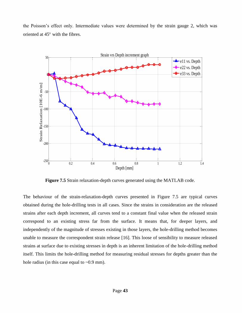
Page 43
the Poisson’s effect only. Intermediate values were determined by the strain gauge 2, which was
oriented at 45 with the fibres.
Figure 7.5 Strain relaxation-depth curves generated using the MATLAB code.
The behaviour of the strain-relaxation-depth curves presented in Figure 7.5 are typical curves
obtained during the hole-drilling tests in all cases. Since the strains in consideration are the released
strains after each depth increment, all curves tend to a constant final value when the released strain
correspond to an existing stress far from the surface. It means that, for deeper layers, and
independently of the magnitude of stresses existing in those layers, the hole-drilling method becomes
unable to measure the correspondent strain release [16]. This loose of sensibility to measure released
strains at surface due to existing stresses in depth is an inherent limitation of the hole-drilling method
itself. This limits the hole-drilling method for measuring residual stresses for depths greater than the
hole radius (in this case equal to ~0.9 mm).
0 0.2 0.4 0.6 0.8 1 1.2 1.4-250
-200
-150
-100
-50
0
50
Depth [mm]
Str
ain
Rela
xati
on [
10E
-6 m
/m]
Strain vrs Depth increment graph
e11 vs. Depth
e22 vs. Depth
e33 vs. Depth

Page 44
0 0.2 0.4 0.6 0.8 1 1.2 1.4-20
0
20
40
60
80
100
Depth [in mm]
Str
ess
es
in [
MP
a]
Sigma1 vs. Depth
Sigma2 vs. Depth
Applied Stress vs. Depth1
Zero Stress vs. Depth1
7.3 Calculated stress distribution and validation of the MATLAB scripts developed
The strain relaxation-depth values shown in Table 7.4 and Figure 7.5 were used as input for the
calculation procedure implemented by the MATLAB scripts developed in this work. Based on the
calibration coefficients previously determined by the finite element method, and shown in Tables 7.1,
7.2 and 7.3, the stresses related with those strain relaxation values can be calculated using the
MATLAB developed codes. Figure 7.6 shows the results obtained from the calculation. For
comparison purposes only the principal stress values calculated by the developed code are shown.
Figure 7.6 Maximum principal stress and minimum principal stress calculated by the MATLAB
scripts developed.
The MATLAB scripts developed to implement the calculation procedure for the determination of
residual stresses can then be validated. During the experimental procedure [45] a tensile stress of 74
MPa was applied to the specimen during the application of the hole drilling technique. It was
expected from the graphs that the results obtained for the principal stress should have an average
value close to 74 MPa and the minimum principal stress approaching zero. According to the results
presented in Fig. 6.2, the maximum principal stress is greater than the experimentally applied stress
over the depth range, while the minimum principal stress is in good agreement with the expected
value.

Page 45
It should be also observed that the maximum principal stress increases during the first depth
increments and stabilize after 0.2 mm depth. This stabilized value should correspond to the applied
calibration stress of 74 MPa. The initial increase of the maximum principal stresses in the graph
suggests there was an error introduced on the results at the beginning of the hole-drilling, i.e., in the
first depth increments. This might happen due to the following main factors:
1. The effect of the drill bit geometry used during hole-drilling;
2. The effect of the positioning or centering of the drill bit. Any eccentricity in respect of the
centre of the strain gauge rosette induces errors;
3. The surface preparation could contribute directly or indirectly to the results;
4. The effect of the numerical uncertainties on the calibration coefficient matrix determination;
5. The thermo-mechanical effects of the cutting procedure can induce parasitic stresses,
especially in the case of fibre reinforce polymers;
6. The limitation of the theoretical approach used for residual stress calculation that was
followed.
Of course, assuming that the measurement system gives accurate strain values, the geometric effects
due to inaccuracies on the hole diameter and hole depth measurements can be disregarded and finally
if the elastic constants of the material were well determined. All these factors are necessary to be
considered and accounted for during the laboratory experiments. The difference and variation in the
maximum residual stress obtained by the MATLAB developed code should certainly be due to these
factors.
For better understand the observed differences between the calculated stresses and the experimental
expected stress value, the observed error as a function of the hole depth was determined. This error is
the relative difference between the maximum principal stress, calculated by the MATLAB scripts
developed, and the expected stress applied during the uniaxial tensile tests (74 MPa). Figure 7.7
presents the results of the error in the determination of the maximum principal stress, since the
observed one in the minimum principal stress can be neglected.

Page 46
0 0.2 0.4 0.6 0.8 1 1.2 1.4-5
0
5
10
15
20
25
Depth [mm]
Perc
en
tage E
rror
err vs. Depth
Figure 7.7 Observed error [] between the maximum principal stress calculated by the MATLAB
scripts developed and the expected stress value
As observed, the error increases in the first depth increments and stabilizes in a value around 23%,
after a hole depth equal to about 0.2 mm. This average error is too high and the reasons for its
appearance should certainly be associated to the factors referred above. A discussion of these factors
and their consequences will be performed in the following. However, according to reference [45],
were the experimental results used in this work are reported, the factors 2 and 3 pointed out above can
be disregarded. Therefore, the discussion will be essentially focused in the reasons 1, 4, 5 and 6,
which should be directly related with the observed differences between the calculated stress and the
experimental value, used as reference.
7.3.1 Effect of the drill bit geometry
The end mills for the incremental hole-drilling technique usually present a small chamfer, which can
affect the hole shape, especially in the first depth increments. This means that the real shape of the
drilled hole is not perfectly cylindrical, as it can be seen in the micrograph of Figure 7.8, taking from
reference [45], where the experimental results used in this work were reported. In Figure 7.8, it is

Page 47
clear that a small portion of the material remains, since it is not cut during hole-drilling due to the end
mill chamfer.
Figure 7.8 Micrograph of drilled hole showing the remaining portion which was not removed [45]
The effect of the chamfer is more pronounced during the first depth increments than in the deeper
ones, since the effect of the chamfer decreases with the increase of the hole size. Its effect on the
results of the stress calculation procedure is related with the fact that, during the numerical simulation
by FEM to obtain the calibration constants Ain, Bin and Cin, a pure cylindrical shape for the hole is
assumed. Therefore, for the first depth increments, the amount of material cut is smaller than if a pure
cylindrical shape is assumed. This effect decreases with the increase of the hole depth. Hence, this
effect can justify the shape of the maximum principal stresses curve shown in Figure 7.6 for the first
depth increments. However, the magnitude of the calculated stress and the high observed error should
associated to other effects.
7.3.2 Effect of the numerical uncertainties on the calibration coefficient matrix determination
It is clear from Figure 7.6 that, for deeper layers, the maximum principal stress remains at values
ranging from 88 MPa to 93 MPa and the minimum stresses settle approximately close to the expected
result. The reason for the average maximum principal stresses being higher than the applied stress,
leading to an error of 23% can be attributed to the numerical uncertainties on the determination of the

Page 48
calibration coefficients matrices Ain, Bin and Cin, respectively, from Tables 7.1, 7.2 and 7.3.
Numerical inaccuracies in their determination affect the calculated results of the stresses, since the
stresses are directly dependent on these coefficients.
7.3.3 Thermo-mechanical effects of the cutting procedure
Considering the results presented in reference [4], the thermo-mechanical effects due to the cutting
procedure should certainly have influence on the experimentally determined strain relaxation-depth
curves, hence affecting the stress calculation using the MATLAB code developed in this work. This
issue should be better investigated in the future. Although the average maximum stress obtained is
higher than the applied stress, the trend presents very promising indicator about the development of
the incremental hole-drilling technique for measuring residual stresses in composite laminates.
Probably, if the real shape of the hole was considered during the finite element analysis, thus
correcting the values of the calibration coefficients, the final stress value could be perfectly constant.
This explanation of the findings should, however, be ascertained in future works.
7.3.4 Limitation of the theoretical approach used for residual stress calculation
Finally, a reference to the theoretical approach followed to develop the MATLAB code [3, 5] should
be done. The theoretical approach followed in this work is based on a simple approach, assuming that
the relieved strain response has a similar trigonometric form to that observed in an isotropic material,
as it can be seen in equation (1). Equation (1) is assumed still to apply, providing that gauges 1 and 3
are aligned along the elastic symmetry directions of the orthotropic material, as it happened in the
composite material previously used. In this case, constant C is an independent calibration constant,
not related to A or B, as it happens for isotropic materials. The use of equation (1) was suggested for
hole-drilling applications by several authors [35, 37]. However, Schajer and Yang [34] have shown
that the use of equation (1) can imply final errors in residual stress calculation because the
displacement field around a hole, in a stressed orthotropic plate, does not have a simple trigonometric
form. Figure 7.9 shows differences that can be expected in the normalized relieved strain around the
hole in an orthotropic plate, comparatively to what is expected in an isotropic material. The
differences increase with the increase of the orthotropy ratio is E11/E22. In the case of the composite
laminate used in this study, this ratio attains 47.

Page 49
Figure 7.9 Angular variation of relieved strain in materials of varying degrees of axial
orthotropy [34].
Disregarding the first depth increments, where the calculated stress values are affected by the end
mill chamfer effect, an error of around 23% was observed. The reason for this level of error should
be studied in the future, regarding the effect of the factors discussed above. However, higher errors
have already been reported by other authors. Schajer and Yang [34], for example, during their
calibration tests, recorded stress-measurement errors in the 10-20-percent range. According to these
authors, this error range was expected to be typical of hole-drilling measurements in orthotropic
laminates. Accuracy of the final results is strongly dependent on the measurement procedure and on
the algorithms adopted to calculate the stresses.
8. CONCLUSIONS
In this work, scripts using MATLAB were developed for determining residual stresses in orthotropic
composite laminates. The theoretical approach followed was proposed by Sicot et al. [3, 5]. This
approach enables to determine the in-depth non uniform residual stress based on the relieved strains
measured during the application of the incremental hole-drilling technique to orthotropic composite

Page 50
laminates. Considering the case of carbon-fibre reinforced polymer (CFRP) specimens, with the
stacking sequence [0o, 90o]5s the necessary calibration coefficient matrices, related with the residual
calculation procedure used, were determined by the finite element method.
For validation purposes, the results obtained in an experimental study, previously performed to the
present work, were used. The strain relaxation-depth curves reported in that study, corresponding to
above mentioned specimens, when subjected to a well-known uniform uniaxial stress, were used as
input data for the MATLAB scripts developed in this work.
Differences between the applied experimental stress (uniform stress) and the calculated one, by using
the MATLAB code developed, were observed. The level of the observed error (~23%) was high, but
similar level of errors were also referred by other authors, reporting experimental calibration
procedures using the hole-drilling technique in composite laminates. Beyond the problems related
with the theoretical approach followed, the source of errors must be well study in the future. The
effect of the chamfer of the drill bits, the thermomechanical effects of the cutting process, the laminar
structure of most orthotropic materials, the uncertainty of local elastic properties and the angular
misalignment of the strain-gauge rosette relative to the material principal elastic directions, are
common sources of errors. However, considering the results obtained in this work, the incremental
hole-drilling can be considered a promising technique for residual stress measurement in composite
laminates.

Page 51
9. REFERENCES
[1] Tsouvalis, N., Margelis, G., Dellis, D., “Residual stresses in composite materials: a review”,
NTUA Report No MAR-R4-3-NTUA-24(2) for MARSTRUCT, January 2009.
[2] Cherouat A., Gong X.L., Sicot O. and Lu J., “Influence of the Residual Stresses on the
mechanical behavior of advanced composite parts”, Journal of Neutron Research, 9(2), 319-
330 (2001).
[3] Sicot, O., Gong, X., Cherouat, A., Lu, J., “Determination of residual stress in composite
laminates using the hole-drilling method”, J. Comp. Mat., 37, 831–844 (2003).
[4] Nobre, J.P., Stiffel, J.H, Nau, A., Outeiro, J., Batista, A.C., Induced drilling strains in glass
fibre reinforced epoxy composites. CIRP Annals Manufacturing Technology, 62(1), 87-90
(2013).
[5] Sicot, O., Gong, X.L., Cherouat, A., Lu J., “Determination of Residual Stress in Composite
Laminates using the Incremental Hole-drilling Method”, J. Comp. Mat., 37, 831–844 (2003).
[6] Parlevliet, P.P., Bersee, H.E.N., Beukers, A, “Residual stresses in thermoplastic composites-
A study of the literature – Part 1: Formation of residual stresses”, Composite: Part A, 37, 1847
– 1857 (2006).
[7] Kim, K., Hahn, H. and Croman, R., “The effect of cooling rate on residual stresses in a
thermoplastic composite”, J. Composire Technol. Res., 11(2), 47-52 (1998).
[8] Daniel, I.M., Liber, Theodore, “Lamination residual stresses in fiber composites”, NASA- CR-
134826, 1975.
[9] While, S.R. and Hahn, H.T. “Process modeling of composites materials: residual stress
development during cure. Part I - Model formulation”, J. Comp. Mat., 26, 402-2422 (1992).
[10] Kharkhadi S, Abrol N, Somani P., Sharma A., Singh T., “Review on Fiber Reinforced
Polymer” International Journal of Combined Research & Development (IJCRD) eISSN: 2321-
225X ; pISSN:2321-2241 Volume: 4; Issue: 6; June -2015
[11] Hinton M.J., Soden P.D., Kaddour A.S., “Failure Criteria in Fibre-Reinforced-Polymer
Composites: The World-Wide Failure Exercise”, Elsevier, 2004.
[12] Masuelli, M. A, Introduction of Fibre-Reinforced Polymers, Polymers and Composites:
Concepts, Properties and Processes. ISBN 978-953-51-0938-9, Published: January 23, 2013
under CC BY 3.0 license. © The Author(s
[13] Reid R. G., Paskaramoorthy R. An extension to classical lamination theory for use with
functionally graded plates, Composite Structures, 93(2): 639-648, 2011

Page 52
[14] Williams G., Trask R., Bond I., “A self-healing carbon fibre reinforced polymer for aerospace
applications”, Part A 38 (2007) 1525–1532. University of Bristol, Queen’s Building, University
Walk, Bristol BS8 1TR, UK, Received 17 May 2006; received in revised form 16 November
2006; accepted 7 January 2007.
[15] Chen B. T. Yeh H. C. & Hobbs C. H. “Size Classification of Carbon Fiber Aerosols, Aerosol
Science and Technology”, (1993), 19:2, 109-120, DOI: 10.1080/02786829308959625
[16] Nobre, J.P., Batista, A.C., Nau, A, Paepegem, W.V, and Scholtes, B., “Using the incremental
hole-drilling technique for measuring residual stresses in fibre-reinforced polymer composites”,
Proc. 5th
European Conference on Composite Materials, Venice, July 2011, Italy, pp 1 – 8,
2011.
[17] Gary S. Schajer, Michael B. Prime, “Use of inverse solutions for residual stress
measurement”, January 2005, Los Alamos National Laboratory, Engineering Sciences and
Applications Division, LA-UR-04-5890, Journal of Engineering Materials and Technology,
128(3), 375-382 (2006).
[18] Patricia P. Parlevliet, Harald E.N. Bersee, Adriaan Beukers, “Residual stresses in thermoplastic
composites – A study of the literature – Part II: Experimenal techniques”, Composites: Part A,
38, 651-665 (2006).
[19] Olabi A.G., Hashmi M.S.J., “Stress relief procedures for low carbon steel (1020) welded
components”, J. Eng. Mater. Tech., 56, 552-562 (1996).
[20] Kandil, F., Lord, J., Fry, A., Grant, P., “A review of residual stress measurement methods, a
guide to technique selection”, NPL Report MATC(A)04, UK, 2001.
[21] Stamatopoulos K., “Measurement of residual stresses in composite materials with the
incremental hole drilling method”, Athens, June 201.
[22] Milbradt K.P., “Ring-method determination of residual stresses”, Proc SESA, 9(1), 63–74
(1951).
[23] Kiel S., “Experimental determination of residual stresses with the ring-core method and an
online measuring system”, Exp. Tech., 16(5): 17–24 (1992).
[24] Ajovalasit, A., Petrucci, G., Zucarello, B. “Determination of Nonuniform Residual Stresses
Using the Ring-Core Method”, J. Eng. Mater. Tech., 118(2), 224-228 (1996).
[25] Prime M.B., “Residual stress measurement by successive extension of a slot: the crack
compliance method”, Appl. Mech. Rev., 52(2), 75–96 (1999).

Page 53
[26] Germaud M.,Cheng W.,Finnie I., Prime M.B., “The compliance method for measurement of
near surface residual stresses analytical background”, J. Eng. Mater. Tech., 119(4), 550–5 55
(1994).
[27] Cheng W.,Finnie I., “Residual stress measurement and the slitting method”. New York:
Springer 2007, ISBN 978-144194241.
[28] Cowley K.D. and Beaumont P.W.R., “The measurement and prediction of residual stresses in
carbon-fibre/polymer composites”, Composites Science and Technology, 57(11), 1445–55
(1997).
[29] Leggatt R.H, Smith D.J., Smith S.D., Faure F., “Development and experimental validation of
the deep hole method for residual stress measurement”, J. Strain Anal., 31(3), 177–186 (1996).
[30] Bateman M.G., Miller O.H.,Palmer T.J., Breen C.E.P.,Kingstonb E.J.,Smith D.J., Pavier M.J.
“Measurement of residual stress in thicksection composite laminates using the deep-hole
method”, Int. J. Mech. Sci., 47, 1718–1739 (2005).
[31] Sachs G. “Der nachweiss innerer spannungen in stangen und rohren”, Zeitschrift fur
Metallkunde, 19, 352–357 (1972).
[32] Oettel R., “The determination of uncertainties in residual stress measurement (using the hole
drilling technique)”, Issue 1, September 2000, Manual of Codes of Practice for the
determination of uncertainties in mechanical tests on metallic materials, Code of Practice No.
15, Standards Measurement & Testing Project No. SMT4-CT97-2165.
[33] ASTM E 837-13, “Standard Test Method For Determining Residual Stresses By Hole Drilling
Gage Method”, ASTM, West Conshohocken, United State, 2013.
[34] Schajer G.S and Yang L., “Residual-Stresses Measurement in Orthotropic Materials Using the
Hole-drilling Method”, Exp. Mech., 34(4), 324-333 (1994).
[35] Bert, C.W. and Thompson, G.L. "A Method for Measuring Planar Residual Stresses in
Rectangularly Orthotropic Materials", J. Comp. Mat., 2(2), 244-253 (1968).
[36] Lake, B.R., Appl, F.J. and Bert, C.W., “An investigation of the hole-drilling technique for
measuring planar residual stress in rectangular orthotropic materials”, Exp Mech., 10 (10), 233-
239 (1970).
[37] Prasad, C.B., Prabhakaran, R. and Thompkins, S., “Determination of Calibration Constants for
the Hole-Drilling Residual Stress Measurement Technique Applied to Orthotropic
Composites”, Composite Structures, Part 1: Theoretical Considerations, 8(2), 105-118 (1987);
Part H: Experimental Evaluations, 8 (3), 165-172 (1987).
[38] Soete, W., “Measurement and Relaxation of Residual Stress”, Sheet Met. Ind., 26(266), 1269–
1281 (1949).

Page 54
[39] Lake, B.R., F.J. and Bert, C.W., “An Investigation of the Hole-Drilling Technique for
Measuring Planar Residual Stress in Rectangular Orthotropic Materials”, Exp. Mech., 10, 233–
239 (1970).
[40] George Margelis, Konstantinos Stamatopoulos, Nicholas Tsouvalis, “Measurement of Residual
Stresses in Typical Marine Composite Materials Using the Incremental Hole Drilling Method”
NTUA Report No MAR-R4-3-NTUA-28(1) for MARSTRUCT, January 2010.
[41] Vishay precision group, “Micro measurements,” Vishay precision group, 01 November 2010.
[Online]. Available: http://www.vishaypg.com/doc?11053. [Accessed 25 November 2015]
[42] N.N: www.hexcel.com, product data - hexPly M18, demand in March 2010.
[43] Tavernier, B., Verbeke, T., Health Monitoring of Carbon-Epoxy Laminates Used in Space
Applications by Means of Embedded Optical Fibers, Master Thesis, Ghent University,
Belgium, 2006.
[44] Jose, S., Ramesh Kumar, R., Jana, M.K., Venkateswara Rao, G., “Intralaminar Fracture
Toughness of a Cross-Ply Laminate and its constituent Sub-Laminates”, Composite Science and
Technology, 61, 1115-1122 (2001).
[45] Nobre, J.P., internal report, University of Coimbra, 2011.
[46] Handbook of Measurement of Residual Stresses. Edited by J. Lu, Society for Experimental
Mechanics (SEM), Bethel, 1996.

Page 55
10. APPENDIX
A1. MATLAB code for the calculation of relieve strains and the corresponding stresses
format short e Amn=[-4.50E-08,-1.10E-06,-1.60E-06,-2.10E-06,-2.40E-06,-2.70E-08,-3.00E06,... -3.20E-06,-3.40E-06,-3.50E-06,-3.60E-06,-3.70E-06,-3.70E-06,-3.80E-06,... -3.80E-06,-3.80E-06,-3.80E-06,-3.90E-06,-3.90E-06,-3.90E-06];
Bmn=[1.67E-10,-9.20E-09,-1.20E-08,-1.50E-08,-1.70E-08,-1.80E-08,-2.00E-08,... -2.20E-08,-2.30E-08,-2.40E-08,-2.60E-08,-2.80E-08,-2.90E-08,-3.00E-08,... -3.20E-08,-3.30E-08,-3.40E-08,-3.50E-08,-3.60E-08,-3.70E-08];
Cmn=[6.33E-11,7.71E-09,-9.73E-09,9.79E-09,9.88E-09,9.63E-09,8.27E-09,... 5.69E-09,4.44E-09,3.33E-09,1.38E-09,-1.30E-10,-2.80E-08,-3.50E-09,... -5.10E-09,-7.10E-09,-8.00E-09,-8.70E-09,-9.80E-09,-1.00E-08];
Depth = [0.0508,0.1016,0.1524,0.2032,0.2540,0.3048,0.3556,0.4064,0.4572,... 0.5080,0.5588,0.6096,0.6604,0.7112,0.7620,0.8128,0.8636,0.9144,... 0.9652,1.0160]';
Emn=[8,0,-11;-77,-4,-12;-83,-12,-10;-87,-20,-9;-126,-26,-6;-167,-30,-3;... -171,-36,-1;-174,-51,1;-188,-55,5;-202,-55,10;-205,-53,11;-206,-66,12;... -210,-61,16;-213,-64,20;-214,-77,21;-215,-77,21;-215,-81,25;-215,-85,29;... -216,-87,29;-216,-85,29];
Emn1 = Emn(:,1)'; Emn2 = Emn(:,2)'; Emn3 = Emn(:,3)';
for n = 1:20 e1 = Emn1(:,n)-sum(Emn1(:,1:1:n-1)); e2 = Emn2(:,n)-sum(Emn2(:,1:1:n-1)); e3 = Emn3(:,n)-sum(Emn3(:,1:1:n-1));
An = Amn(1,n); Bn = Bmn(1,n); Cn = Cmn(1,n);
theta=0.5*atan((Cn*(e3-e1)-Bn*(2*e2-e1-e3))/(Cn*(2*e2-e1-e3)+Bn*(e3-e1))); Sigma1 = (e1*(An-Bn*sin(2*theta)+Cn*cos(2*theta))-e2*(An-Bn*cos(2*theta)-
Cn*sin(2*theta)))...
/((2*An*Bn)*(sin(2*theta)+cos(2*theta))+(2*An*Cn)*(sin(2*theta)+cos(2*t
heta))); Sigma2=(e1*(An+Bn*sin(2*theta)Cn*cos(2*theta))+e2*(An+Bn*cos(2*theta)+Cn*sin(2*th
eta))).../((2*An*Bn)*(sin(2*theta)+cos(2*theta))+(2*An*Cn)*(sin(2*theta
)+cos(2*theta)));
disp([Sigma1,Sigma2]) end

Page 56
A2. MATLAB code for plotting of Stresses with Depth
% Plot of the first set of strain values format short e Sigma1=[-0.0309e+10,-0.1737e+09, 0.0655e+09, -0.0752e+09,-0.0111e+09,... -0.2552e+09, -0.4121e+09, -0.0339e+10,-0.0478e+10,-0.0347e+10,... -0.0333e+10,-0.0079e+10,-0.0089e+10,-0.0038e+10,-0.0275e+10,... -0.0187e+10,-0.0140e+10,0.0165e+10,-0.0170e+10,-0.0182e+10]'.*10^-8;
Sigma2=[0.7143e+10,0.8155e+10,0.8577e+10,8.9421e+09,9.1271e+09,... 0.9152e+10,9.2379e+09, 0.9114e+10, 0.9241e+10,0.9133e+10,... 0.9241e+10,0.9208e+10,0.9243e+10,0.9111e+10,0.9074e+10,... 0.9011e+10,0.9090e+10,0.9029e+10, 0.8758e+10,0.8295e+10]'.*10^-8;
Sig1=[74,74,74,74,74,74,74,74,74,74,74,74,74,74,74,74,74,74,74,74,74]';
Sig2=[0,0,0,0,0,0,0,0,0,0,0,0,0,0,0,0,0,0,0,0,0]';
Depth = [0.0508,0.1016,0.1524,0.2032,0.2540,0.3048,0.3556,0.4064,0.4572,... 0.5080,0.5588,0.6096,0.6604,0.7112,0.7620,0.8128,0.8636,0.9144,... 0.9652,1.0160]';
Depth1 = [0,0.0508,0.1016,0.1524,0.2032,0.2540,0.3048,0.3556,0.4064,0.4572,... 0.5080,0.5588,0.6096,0.6604,0.7112,0.7620,0.8128,0.8636,0.9144,... 0.9652,1.0160]';
plot(Depth,Sigma1,'x--',Depth,Sigma2,'og--',Depth1,Sig1,Depth1,Sig2),grid xlabel('Depth [in mm]') ylabel(' Stresses in [MPa]')
A3. MATLAB code for plotting of the strains with depth
%The plot of first set of strain values
A=[8,0,-11;-77,-4,-12;-83,-12,-10;-87,-20,-9;-126,-26,-6;-167,-30,-3;... -171,-36,-1;-174,-51,1;-188,-55,5;-202,-55,10;-205,-53,11;-206,-66,12;... -210,-61,16;-213,-64,20;-214,-77,21;-215,-77,21;-215,-81,25;-215,-85,29;... -216,-87,29;-216,-85,29]';
e11=[0,3,-77,-90,-100,-126,-160,-171,-174,-188,-202,-205,-206,-210,-213,-214,... -215,-215,-215,-216,-216]'; e22=[0,-4,-12,-20,-26,-30,-36,-51,-55,-55,-53,-66,-61,-64,-77,-77,-81,-85,-87,-
85,-85]'; e33=[0,-11,-12,-10,-9,-6,-3,-1,1,5,10,11,12,16,20,21,21,25,29,29,29]';
Depth = [0,0.0508,0.1016,0.1524,0.2032,0.2540,0.3048,0.3556,0.4064,0.4572,... 0.5080,0.5588,0.6096,0.6604,0.7112,0.7620,0.8128,0.8636,0.9144,... 0.9652,1.0160]';
plot(Depth,e11,'x--',Depth,e22,'g--',Depth,e33,'or--'),grid xlabel('Depth [mm] ') ylabel('Strain Relaxation [micro m/m]') title('Strain vrs Depth increment graph')

Page 57
A4. MATLAB code for plotting of Percentage Errors with depth
% Perentage error format short e err=[-3.4730e+00,1.0203e+01,1.5905e+01,2.0839e+01,2.3339e+01,2.3676e+01,... 2.3836e+01,2.3162e+01,2.2932e+01,2.3419e+01,2.3878e+01,2.3432e+01,... 2.3905e+01,2.3122e+01,2.2622e+01,2.1770e+01,2.1838e+01,2.1014e+01,... 1.4297e+01,1.2095e+01]';
Depth = [0.0508,0.1016,0.1524,0.2032,0.2540,0.3048,0.3556,0.4064,0.4572,... 0.5080,0.5588,0.6096,0.6604,0.7112,0.7620,0.8128,0.8636,0.9144,... 0.9652,1.0160]';
plot(Depth,err,'o--'),grid
xlabel('Depth [mm]') ylabel('Percentage Error')
Recommended


![Prediction of welding residual stresses using machine ... · characterise the distribution of residual stresses in structural welds [6, 7]. With the development of residual stress](https://img.pdfslide.us/doc/110x75/5fa3f63f3be93a3412525cc3/prediction-of-welding-residual-stresses-using-machine-characterise-the-distribution.jpg)