DETERMINATION OF ELASTIC CONSTANTS FOR GEOSYNTHETICS USING IN-
AIR BIAXIAL TENSION TESTS
by
Henry Nathaniel Haselton
A thesis submitted in partial fulfillment of the requirements for the degree
of
Master of Science
in
Civil Engineering
MONTANA STATE UNIVERSITY
Bozeman, Montana
April 2018

©COPYRIGHT
by
Henry Nathaniel Haselton
2018
All Rights Reserved

ii
ACKNOWLEDGEMENTS
I would like to thank my girlfriend Linnaea, my parents Eliza and George, my
sister Sarah and all of my friends for being very supportive and helpful to me throughout
all my years of school and the writing this thesis. I would like to thank Dr. Steve Perkins
for his great contributions, continued assistance and advice throughout the entire research
and writing process.
I would like to thank Eli Cuelho for designing and building the biaxial testing
device as well as his advice pertaining to using the device and other equipment at the
Western Transportation Institute (WTI). I would like to thank Stephen Valero and Hanes
Geo for providing the geosynthetics used for testing. I would like to thank the folks at
WTI for allowing us to use the lab facilities and store the geosynthetic materials. I would
like to thank Beker Cuelho for assisting me with the initial lab testing and showing me
how to operate testing equipment. I would like to thank Emily Schultz for all of the lab
testing she conducted. I would like to thank Dr. Mark Owkes for his assistance with
MATLAB and the least squares approximation technique.
I would like to thank the funding sources, the National Science Foundation
(award number 1635029) and the Geosynthetic Institute for providing funding used
during the first year of this project. I would also like to thank the College of Engineering
for a graduate teaching assistant position for my second year of graduate school.
iii
TABLE OF CONTENTS
1. INTRODUCTION .......................................................................................................... 1
Background ..................................................................................................................... 1
Previous Work on Geosynthetics .................................................................................... 2
Scope of Work ................................................................................................................ 3
2. LITERATURE REVIEW ............................................................................................... 4
Introduction ..................................................................................................................... 4
Uniaxial Testing of Geosynthetics .................................................................................. 4
Biaxial Testing of Structural Membranes and Fabrics ................................................... 7
Biaxial Testing of Geosynthetics .................................................................................. 16
Synthesis of Literature Review ..................................................................................... 21
3. THEORY ...................................................................................................................... 22
Constitutive Equations .................................................................................................. 22
Numerical Methods....................................................................................................... 24
4. TESTING PROCEDURE DEVELOPMENT............................................................... 31
Testing Procedure Methodology ................................................................................... 31
Uniaxial Testing Overview ........................................................................................... 32
Uniaxial Testing Device................................................................................................ 33
Stress Relaxation........................................................................................................... 35
Creep under Sustained Load ......................................................................................... 36
Effect of Stress Relaxation and Creep Duration ........................................................... 38
5. UNIAXIAL TESTING RESULTS AND INTERPRETATION .................................. 40
Uniaxial Testing Results ............................................................................................... 40
iv
TABLE OF CONTENTS CONTINUED
Cyclic Stress Relaxation ............................................................................................... 40
Monotonic Stress Relaxation ........................................................................................ 49
Cyclic Creep.................................................................................................................. 60
Monotonic Creep........................................................................................................... 63
Analysis of Uniaxial Testing ........................................................................................ 70
Conclusions from Uniaxial Testing .............................................................................. 78
6. BIAXIAL TESTING..................................................................................................... 80
Biaxial Testing Methods ............................................................................................... 80
Biaxial Testing Device.................................................................................................. 82
Testing Setup................................................................................................................. 85
Testing Procedure ......................................................................................................... 94
Biaxial Testing Results ................................................................................................. 95
7. SUMMARY AND RECOMMENDATIONS............................................................. 132
Summary of Testing and Analysis .............................................................................. 132
Recommendations for Future Testing......................................................................... 133
REFERENCES CITED................................................................................................... 138
APPENDICES ................................................................................................................ 141
APPENDIX A: Nonlinear Least Squares Approximation for
Solving Elastic Constants...………………………………………………...142
APPENDIX B: Load per unit width vs. Strain Plots for Biaxial Test……...146
APPENDIX C: Draft of Testing Standard for Determination of Elastic Constants for Geosynthetics using In-Air Biaxial Tension Tests…..181
v
LIST OF TABLES
Table Page
1. Elastic Constants Using Different Calculation Methods ................................ 15
2. Summary of Uniaxial Testing ......................................................................... 39
3. Cyclic Stress Relaxation Tests on a Biaxial Geogrid ..................................... 44
4. Cyclic Stress Relaxation Tests on a Woven Geotextile .................................. 45
5. Cyclic Stress Relaxation at 4.0 % Strain after 24 Hours ................................ 49
6. Monotonic Stress Relaxation Tests on a Biaxial Geogrid .............................. 52
7. Monotonic Stress Relaxation Tests on a Woven Geotextile ........................... 52
8. Monotonic Stress Relaxation at 4.0 % Strain after 24 Hours ......................... 56
9. Monotonic Stress Relaxation at 4.0 % Strain ................................................. 58
10. Cyclic Creep at 4.0 % Strain after 24 Hours................................................... 61
11. Modulus from Monotonic Creep Test on a Woven Geotextile ....................... 64
12. Modulus from Monotonic Creep Tests at 4.0 % Strain at 24 Hours for a Woven Geotextile ................................................................................... 66
13. Modulus from Monotonic Creep Tests at 4.0 % Strain at 24 hours ............... 66
14. Monotonic Stress Creep at 4.0 % Strain ......................................................... 68
15. Comparing Average Modulus Values from Cyclic and Monotonic
Stress Relaxation (10 Min. Hold) on a Biaxial Geogrid ................................. 73
16. Comparing Average Modulus Values from Cyclic and Monotonic Stress Relaxation (10 Min. Hold) on a Woven Geotextile ............................. 73
17. Comparing Average Modulus Values from Cyclic and Monotonic Stress Relaxation (20 Min. Hold) on a Biaxial Geogrid ................................. 74
vi
LIST OF TABLES CONTINUED
Table Page
18. Comparing Average Modulus Values from Cyclic and Monotonic Stress Relaxation (20 Min. Hold) on a Woven Geotextile ............................. 74
19. Comparing Modulus Values from 24 Hr. Cyclic and Monotonic
Stress Relaxation on a Biaxial Geogrid .......................................................... 75
20. Comparing Modulus Values from 24 Hr. Cyclic and Monotonic
Stress Relaxation on a Woven Geotextile....................................................... 75
21. Comparing Modulus Values from 24 Hr. Cyclic and Monotonic
Stress Relaxation and Creep on a Biaxial Geogrid ......................................... 75
22. Comparing Modulus Values from 24 Hr. Cyclic and Monotonic Stress Relaxation and Creep on a Woven Geotextile ..................................... 75
23. Comparing Modulus Values from 20 Min. and 24 Hr. Monotonic Stress Relaxation on a Biaxial Geogrid .......................................................... 77
24. Comparing Modulus Values from 20 Min. and 24 Hr. Monotonic
Stress Relaxation on a Woven Geotextile....................................................... 77
25. Comparing Modulus Values from 20 Min. and 24 Hr. Monotonic
Creep on a Biaxial Geogrid............................................................................. 77
26. Comparing Modulus Values from 20 Min. and 24 Hr. Monotonic
Creep on a Woven Geotextile ......................................................................... 77
27. Comparing Modulus Values from 20 Min. Monotonic Creep and Relaxation, 24 Hr. Monotonic and Cyclic Stress Relaxation and Creep on a Biaxial Geogrid............................................................................. 78
28. Comparing Modulus Values from 20 Min. Monotonic Creep and
Relaxation, 24 Hr. Monotonic and Cyclic Stress Relaxation and Creep on a Biaxial Geogrid............................................................................. 78
29. Summary of Materials Tested Biaxially ......................................................... 81
30. Strain Rate of Mode 1 Trials on Geogrid A.................................................. 100
vii
LIST OF TABLES CONTINUED
Table Page
31. Outlier Data for Geogrid A ........................................................................... 109
32. Average Modulus of Elasticity with respect to Load Step from Least Squares Stress and Strain Minimization for XMD of Geogrid A ....... 113
33. Average Modulus of Elasticity with respect to Load Step from Least Squares Stress and Strain Minimization for MD of Geogrid A .................... 114
34. Average Poisson’s Ratio with respect to Load Step from Least
Squares Stress and Strain Minimization for XMD-MD of Geogrid A ......... 114
35. Average Poisson’s Ratio with respect to Load Step from Least
Squares Stress and Strain Minimization for MD-XMD of Geogrid A ......... 114
36. R2 values for Fit of Calculated Stress Values to Measured Stress Values .... 116
37. Elastic Constants for Geogrid A at Low Levels of Strain ............................ 119
38. Elastic Constants by Load Step for All Geogrids ......................................... 123
39. Elastic Constants for Low Levels of Strain for Geogrids ............................. 127
40. Elastic Constants by Load Step for All Geotextiles...................................... 130
41. Table 1 Elastic Constants for Low Levels of Strain for
Geotextiles……………………………………………………………...…..131
viii
LIST OF FIGURES
Figure Page
1. Cyclic and monotonic wide-width tension tests on biaxial geogrid, machine direction (Cuelho et al. 2005) ............................................................. 6
2. Cyclic tensile modulus versus permanent strain, machine direction
(Cuelho et al. 2005)........................................................................................... 7
3. Left: Biaxial Testing Device Used for Testing High-Strength Fabrics
Right: Strain Field from Equal Loading along both axes (Krause & Bartolotta, 2001)……...…………………………………….……..8
4. Cruciform Shaped Biaxial Sample with Slits along Cruciform Arms (Bridgens and Gosling, 2003)……………………...…………………...9
5. Stress Distribution in Interior Portion of Biaxial Sample
(Bridgens and Gosling, 2003)…………………………………………..……10
6. Biaxial Sample Dimensions for Japanese Testing Standard
(MSAJ, 1995).................................................................................................. 12
7. Biaxial Testing Device used for Sustained Loading Tests on Biaxial
Geogrids (Kupec & McGown, 2004).............................................................. 17
8. Results from Biaxial and Uniaxial Sustained Loading Tests (Kupec & McGown, 2004) ............................................................................. 18
9. Biaxial Geogrid Specimen for Biaxial Test (McGown et al., 2004) .............. 19
10. Biaxial and Uniaxial Constant Rate of Strain Tests on a Biaxial Geogrid (McGown et al., 2004) ...................................................................... 20
11. Uniaxial Testing Device.................................................................................. 34
12. Curtis Geo-Grips Used for Wide Width Tensile Tests ................................... 35
13. Cyclic Stress Relaxation Test on a Biaxial Geogrid ....................................... 41
14. Cyclic Stress Relaxation Test on Woven Geotextile ...................................... 41
15. Equivalent Force per unit Width Equation (ASTM 2016).............................. 42
ix
LIST OF FIGURES CONTINUED
Figure Page
16. Modulus vs. Strain for Cyclic Stress Relaxation Tests on a Biaxial Geogrid ............................................................................................... 45
17. Modulus vs. Strain for Cyclic Stress Relaxation Tests on a
Woven Geotextile ........................................................................................... 46
18. Cyclic Stress Relaxation 24 hr. Test on a Biaxial Geogrid ............................. 47
19. Cyclic Stress Relaxation 24 hr. Test on a Woven Geotextile ......................... 47
20. Modulus at 4.0 % Strain for 24-hour Cyclic Stress Relaxation Test on a Biaxial Geogrid ....................................................................................... 48
21. Modulus at 4.0 % Strain for 24-hour Cyclic Stress Relaxation Test
on a Woven Geotextile.................................................................................... 49
22. Monotonic Stress Relaxation (10-minute hold time) Test on a
Biaxial Geogrid ............................................................................................... 50
23. Monotonic Stress Relaxation Test (10-minute holds) on a
Woven Geotextile ........................................................................................... 51
24. Monotonic Stress Relaxation Test (20-minute hold time) on a Biaxial Geogrid ............................................................................................... 53
25. Monotonic Stress Relaxation Test (20-minute hold time) on a Woven Geotextile ........................................................................................... 53
26. Average Modulus from Monotonic Stress Relaxation Tests on a
Biaxial Geogrid ............................................................................................... 54
27. Average Modulus from Monotonic Stress Relaxation Tests on a
Woven Geotextile ........................................................................................... 54
28. Monotonic Stress Relaxation 24 hr. Test on a Biaxial Geogrid ..................... 55
29. Monotonic Stress Relaxation 24 hr. Test on a Woven Geotextile .................. 56
30. Monotonic Relaxation 1 hr. Test on Biaxial Geogrid ..................................... 57
x
LIST OF FIGURES CONTINUED
Figure Page
31. Monotonic Relaxation 1 hr. Test on Woven Geotextile ................................. 58
32. Monotonic Stress Relaxation Test at 4.0 % Strain over 60 Minutes on a Biaxial Geogrid ......................................................................... 59
33. Monotonic Stress Relaxation Test at 4.0 % Strain over 60 Minutes on a Woven Geotextile...................................................................... 59
34. Cyclic Creep 24 hr. Test on a Biaxial Geogrid ............................................... 60
35. Cyclic Creep 24 hr. Test on a Woven Geotextile ........................................... 61
36. Modulus from Cyclic Creep Tests on Biaxial Geogrid .................................. 62
37. Modulus from Cyclic Creep Tests on Woven Geotextile ............................... 62
38. Monotonic Creep on a Woven Geotextile....................................................... 63
39. Modulus from Monotonic Creep Tests on a Woven Geotextile ..................... 64
40. Monotonic Creep 24 hr. Test on a Biaxial Geogrid ........................................ 65
41. Monotonic Creep 24 hr. Test on a Woven Geotextile .................................... 66
42. Monotonic Creep 1 hr. Test on Biaxial Geogrid............................................. 67
43. Monotonic Creep 1 hr. Test on Woven Geotextile ......................................... 68
44. Monotonic Creep Test at 4.0 % Strain over 60 Minutes on a
Biaxial Geogrid ............................................................................................... 69
45. Monotonic Creep Test at 4.0 % Strain over 60 Minutes on a
Woven Geotextile ........................................................................................... 69
46. Comparison of Modulus Values from Cyclic Relaxation and
Monotonic Relaxation Tests on a Biaxial Geogrid ......................................... 71
47. Comparison of Modulus Values from Cyclic Relaxation, Monotonic Relaxation and Monotonic Creep Tests on a Woven Geotextile .................... 71
xi
LIST OF FIGURES CONTINUED
Figure Page
48. Biaxial Testing Device at MSU/WTI.............................................................. 82
49. Biaxial Testing Device Bottom Half............................................................... 83
50. Biaxial Testing, Load Plate and Stationary Plate ............................................ 84
51. Woven Geotextile in End Clamp .................................................................... 86
52. Biaxial Testing Device with a Biaxial Geogrid Setup .................................... 87
53. Biaxial Testing Device with a Woven Geotextile Sample .............................. 88
54. LVDT Attachment for Biaxial Geogrid Samples ........................................... 90
55. LVDT Attachment for Biaxial Woven Geotextile Samples ........................... 91
56. Biaxial Testing Device, Bolt for Applying Seating Load ............................... 92
57. Mode 1 Test on Geogrid A ............................................................................. 96
58. Mode 2 Test on Geogrid A ............................................................................. 97
59. Mode 3 Test on Geogrid A ............................................................................. 98
60. Mode 1 Test on Geogrid A, Zoomed in on Load Step 1 ............................... 100
61. Mode 2 Test on Geogrid A, Zoomed in on Load Step 5 ............................... 102
62. Mode 3 Test on Geogrid A, Zoomed in on Load Step 6 ............................... 102
63. Mode 2 Test on Geogrid A, Zoomed in on Load Step 6 Y-Direction .......... 103
64. Mode 3 Test on Geogrid A, Zoomed in on Load Step 5 X-Direction .......... 104
65. Pseudo Modulus vs. Load Step for Mode 1 Tests on Geogrid A ................. 105
66. Pseudo Modulus vs. Strain for Mode 1 Tests on Geogrid A ........................ 105
67. Pseudo Modulus vs. Load Step for Mode 2 Tests on Geogrid A ................. 106
xii
LIST OF FIGURES CONTINUED
Figure Page
68. Pseudo Modulus vs. Strain for Mode 2 Tests on Geogrid A ........................ 107
69. Pseudo Modulus vs. Load Step for Mode 3 Tests on Geogrid A ................. 107
70. Pseudo Modulus vs. Strain for Mode 3 Tests on Geogrid A ........................ 108
71. Modulus of Elasticity in Both Directions for Geogrid A by Load Step ....... 111
72. Poisson’s Ratio in Both Directions for Geogrid A by Load Step ................. 112
73. Comparision of Calculated and Measured Stress Values Using Elastic Constants for Each Load Step for Geogrid A ............................................... 116
74. Modulus of Elasticity in Both Directions for Geogrid A.............................. 118
75. Poisson’s Ratio in Both Directions for Geogrid A ....................................... 119
76. Comparision of Calculated and Measured Stress Values Using Single Set of Elastic Constants for Geogrid A.............................................. 120
77. Modulus of Elasticity, E1, vs. Load Step for All Geogrids ........................... 121
78. Modulus of Elasticity, E2, vs. Load Step for All Geogrids ........................... 122
79. Poisson’s Ratio, ν12, vs. Load Step for All Geogrids .................................... 122
80. Poisson’s Ratio, ν21, vs. Load Step for All Geogrids .................................... 123
81. Modulus vs. Strain for Geogrid A from Different Types of Loading
(Eli Cuelho & Ganeshan, 2004) .................................................................... 126
82. Modulus of Elasticity, E1, vs. Load Step for All Geotextiles ....................... 128
83. Modulus of Elasticity, E2, vs. Load Step for All Geotextiles ....................... 128
84. Poisson’s Ratio, ν12, vs. Load Step for All Geotextiles ................................ 129
85. Poisson’s Ratio, ν21, vs. Load Step for All Geotextiles ................................ 129
xiii
LIST OF FIGURES CONTINUED
Figure Page
86. Geogrid A Mode Trial 1................................................................................ 147
87. Geogrid Mode 1 Trial 2 ................................................................................ 147
88. Geogrid A Mode 1 Trial 3............................................................................. 148
89. Geogrid A Mode 1 Trial 4............................................................................. 148
90. Geogrid A Mode 1 Trial 5............................................................................. 149
91. Geogrid A Mode 1 Trial 1............................................................................. 149
92. Geogrid A Mode 2 Trial 1............................................................................. 150
93. Geogrid A Mode 2 Trial 2............................................................................. 150
94. Geogrid A Mode 2 Trial 3............................................................................. 151
95. Geogrid A Mode 2 Trial 4............................................................................. 151
96. Geogrid A Mode 2 Trial 5............................................................................. 152
97. Geogrid A Mode 2 Trial 6............................................................................. 152
98. Geogrid A Mode 3 Trial 1............................................................................. 153
99. Geogrid A Mode 3 Trial 2............................................................................. 154
100. Geogrid A Mode 3 Trial 3 .......................................................................... 154
101. Geogrid A Mode 3 Trial 4 .......................................................................... 155
102. Geogrid A Mode 3 Trial 5 .......................................................................... 155 103. Geogrid A Mode 3 Trial 6 .......................................................................... 156
104. Geogrid B Mode 1 Trial 2........................................................................... 156
105. Geogrid B Mode 1 Trial 3........................................................................... 157
xiv
LIST OF FIGURES CONTINUED
Figure Page
106. Geogrid B Mode 1 Trial 4............................................................................ 157
107. Geogrid B Mode 2 Trial 1............................................................................ 158 108. Geogrid B Mode 3 Trial 2............................................................................ 158
109. Geogrid C Mode 1 Trial 1............................................................................ 159
110. Geogrid C Mode 1 Trial 2............................................................................ 159
111. Geogrid C Mode 1 Trial 3............................................................................ 160
112. Geogrid C Mode 2 Trial 1............................................................................ 160 113. Geogrid C Mode 2 Trial 2............................................................................ 161
114. Geogrid C Mode 3 Trial 1............................................................................ 161
115. Geogrid D Mode 1 Trial 3 ........................................................................... 162
116. Geogrid D Mode 1 Trial 4 ........................................................................... 162
117. Geogrid D Mode 1 Trial 5 ........................................................................... 163 118. Geogrid D Mode 2 Trial 1 ........................................................................... 163
119. Geogrid D Mode 2 Trial 2 ........................................................................... 164
120. Geogrid D Mode 2 Trial 4 ........................................................................... 164
121. Geogrid D Mode 3 Trial 1 ........................................................................... 165
122. Geogrid D Mode 3 Trial 2 ........................................................................... 165 123. Geogrid E Mode 1 Trial 1 ............................................................................ 166
124. Geogrid E Mode 1 Trial 2 ............................................................................ 166
125. Geogrid E Mode 1 Trial 3 ............................................................................ 167
xv
LIST OF FIGURES CONTINUED
Figure Page
126. Geogrid E Mode 2 Trial 1 ............................................................................ 167
127. Geogrid E Mode 2 Trial 3 ............................................................................ 168 128. Geogrid E Mode 3 Trial 1 ............................................................................ 168
129. Geogrid E Mode 3 Trial 2 ............................................................................ 169
130. Geogrid F Mode 1 Trial 1 ............................................................................ 169
131. Geogrid F Mode 1 Trial 2 ............................................................................ 170
132. Geogrid F Mode 1 Trial 3 ............................................................................ 170 133. Geogrid F Mode 1 Trial 4 ............................................................................ 171
134. Geogrid F Mode 1 Trial 5 ............................................................................ 171
135. Geogrid F Mode 2 Trial 1 ............................................................................ 172
136. Geogrid F Mode 3 Trial 1 ............................................................................ 172
137. Geogrid F Mode 3 Trial 3 ............................................................................ 173 138. Geogrid F Mode 3 Trial 4 ............................................................................ 173
139. Geotextile A Mode 1 Trial 1 ........................................................................ 174
140. Geotextile A Mode 1 Trial 2 ........................................................................ 174
141. Geotextile A Mode 1 Trial 3 ........................................................................ 175
142. Geotextile A Mode 2 Trial 1 ........................................................................ 175 143. Geotextile A Mode 3 Trial 1 ........................................................................ 176
144. Geotextile A Mode 3 Trial 2 ........................................................................ 176
145. Geotextile B Mode 1 Trial 4 ........................................................................ 177
xvi
LIST OF FIGURES CONTINUED
Figure Page
146. Geotextile B Mode 1 Trial 5 ......................................................................... 177
147. Geotextile B Mode 1 Trial 6 ......................................................................... 178 148. Geotextile B Mode 1 Trial 7 ......................................................................... 178
149. Geotextile B Mode 1 Trial 1 ......................................................................... 179
150. Geotextile B Mode 2 Trial 2 ......................................................................... 179
151. Geotextile B Mode 3 Trial 1 ......................................................................... 180
152. Biaxial Testing Specimen…………...……………………………………...184 153. Determination of Pseudo Modulus for Mode 1 Loading...…………………188
154. Pseudo Modulus vs. Load Step for Mode 1 Loading…………...…………..189
xvii
ABSTRACT
Geosynthetics are polymeric membranes used for structural reinforcement for
many geotechnical applications such as reinforced pavement. Geosynthetics have been
shown to increase the service life of roadways in a variety of field tests. The knowledge of geosynthetics and design methodologies could be improved with a better
understanding of geosynthetic material properties. To better understand how geosynthetics perform in field loading situations, geosynthetic tensile resilient material properties are needed. The properties of geosynthetics of interest for this thesis are the
resilient tensile modulus of elasticity and Poisson’s Ratio (elastic constants) in both material directions. Modulus of elasticity has been traditionally calculated using wide-
width uniaxial tests, which is a poor representation of field loading conditions due to the unrestrained sides of the material. Biaxial tension tests are a better representation of field loading conditions and thus were implemented for determination of elastic constants
pertaining to different geosynthetic materials. Biaxial tension tests were performed on cruciform shaped samples using a custom device built by the Western Transportation
Institute at Montana State University to test geosynthetic samples. A biaxial testing procedure was created using conclusions from a uniaxial testing program implemented to examine the resilient response of geosynthetics after being subjected to four types of
loading (cyclic stress relaxation, monotonic stress relaxation, cyclic creep and monotonic creep) over different durations of time. The conclusions of the uniaxial testing program,
the available literature and ASTM D7556 were synthesized to create a biaxial testing procedure. Biaxial tension tests were performed in three modes of loading to simulate loading conditions and loadings where a geosynthetic experiences loading in both
directions simultaneously. The biaxial tension tests generated stress and strain data used to calculate the elastic constants of six biaxial geogrids and two woven geotextiles. The
elastic constants were calculated using an orthotropic linear elastic constitutive model with a least squares approximation. The elastic constants calculated for each geosynthetic material were shown to represent the resilient behavior of geosynthetics in different field
loading situations with more realistic boundary conditions than previous uniaxial tests used to characterize the resilient response of geosynthetics.

1
CHAPTER ONE
INTRODUCTION
Background
Geosynthetics are defined by ASTM D4439 as
A planar product manufactured from polymeric material used with soil,
rock, earth, or other geotechnical engineering related material as an integra l part of human-made project, structure, or system (ASTM, 2017).
Geosynthetics are currently used in many geotechnical applications for structural
reinforcement of soil. Common geosynthetic applications include retaining structures,
roads, constructed slopes and load transfer platforms. For roadways, geosynthetics are
placed at the bottom of or within the base course layer to provide reinforcement. This
reinforcement can allow less base course to be used and/or can extend the service life of
the roadway (Cuelho, 1998).
The performance of geosynthetics used for structural reinforcement of soil is
dependent on tensile strength as well as other mechanisms (Koerner, 2012). In roads, as
well as other applications, geosynthetics are subjected to a biaxial mode of loading,
meaning the material experiences load simultaneously in both principal material
directions. In applications such as long retaining walls, the direction perpendicular to the
retaining wall face experiences loading, while the orthogonal direction is a direction of
plane strain. Load still develops in this direction due to the Poisson effect, which impacts
the stiffness and strength of the material in the direction being loaded.
2
Geosynthetics in applications such as roadways, experience repetitive loading
over long durations of time that make the material experience some combination of stress
relaxation and creep. The resilient response of the geosynthetic when loaded in tension
repetitively is of interest in these applications.
Previous Work on Geosynthetics
The tensile properties of geosynthetics have primarily been studied using wide
width tensile tests and other types of uniaxial load devices. Geotextiles have been tested
for quality control as well as material properties using the wide-width strip method
outlined in ASTM D4595. Geogrids have been tested in a similar manner to determine
tensile properties with the Multi-Rib Tensile Method outlined by ASTM D6637. Wide-
width cyclic uniaxial tension tests have been performed in the past in order to simulate
loads experienced by geosynthetics in road applications (Cuelho et al., 2005). This test
was created to obtain more realistic geosynthetic material properties for pavement design
and is outlined by ASTM D7556. These tests, as well as all types of uniaxial tests, are
less representative of field loading conditions because of the unrestrained sides of the
material. The results from uniaxial tests are often used simply as index tests because they
cannot accurately characterize how geosynthetics will perform in field applications.
Some design methods for field applications use load-strain material
models for geosynthetics based on orthotropic linear elastic models. These
orthotropic linear elastic models and other more advanced orthotropic elastic-
plastic models have not been calibrated from appropriate tensile tests involving
3
controlled stress and strain boundaries. In order to calibrate these material models
with appropriate test data, an advanced testing device that can apply loads
simultaneously in two material directions is necessary. A biaxial testing device of
this nature has been built by the Western Transportation Institute at Montana State
University and was used for this research project.
Scope of Work
The goal of this research is to conduct biaxial tests in a manner that simulates a
resilient load-strain response of geosynthetics that is representative of their response in
applications such as wheel loading in roads. Initially uniaxial wide width tensile tests
were performed on a woven geotextile and a geogrid to create a procedure for the
experimental biaxial testing device. Biaxial tests were then conducted to determine elastic
constants for an orthotropic linear elastic constitutive model of these materials. The
material properties desired from biaxial tests were the modulus of elasticity in both
principal directions and the in-plane Poisson’s ratio.

4
CHAPTER TWO
LITERATURE REVIEW
Introduction
Biaxial tests have been used for determining material response and properties on a
variety of materials in the past. Many structural membranes used for building materials
have been tested using biaxial samples and yielded useful results. For geosynthetics, far
fewer biaxial tests have been conducted and have yielded inconclusive results. In the
past, different types of uniaxial tests have been performed on geosynthetics because a less
complex testing device is necessary. Literature from uniaxial testing on geosynthetics
was examined as well for this literature review.
Uniaxial Testing of Geosynthetics
A variety of uniaxial testing procedures have been developed for both geogrids
and geotextiles for the application of structural reinforcement of soil. Some tests are
simply used as index tests while others are intended to provide insight into the
performance of the geosynthetic in field applications. Tensile tests on geosynthetics can
provide information such as the tensile stress vs. strain, ultimate strength, strain at failure
and modulus of elasticity (Koerner, 2012). Several testing standards exist for determining
the in-air material properties for geosynthetics including ASTM D1682, D751, D4632,
D4595, D6637 and D7556 (Koerner, 2012). For determination of the modulus of
elasticity, it is desirable to use significantly wide samples to reduce the effects of necking
5
that occurs in uniaxial tension tests. The use of wide samples in comparison to their
length reduces the Poisson effect (necking) of the sample and thus allows for more
realistic stress and strain measurements. This concept was used for testing geotextiles to
calculate modulus values because geotextiles (especially nonwovens) are susceptible to
necking.
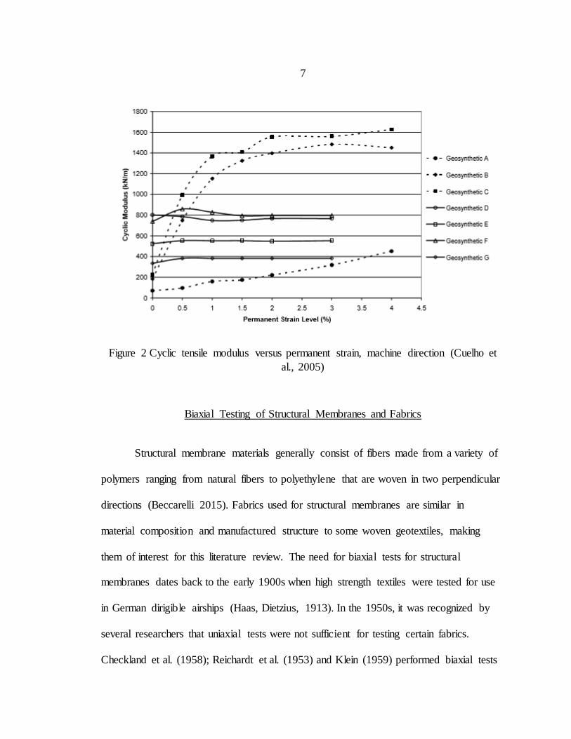
Cuelho et al. (2005) examined the resilient response of geosynthetics subjected to
repetitive loading to simulate field loading conditions to which geosynthetics are
subjected in reinforced flexible pavements. Cyclic wide width tensile tests were
performed for this study on a variety of geotextiles and geogrids. The objective of this
study was to document the modulus or stiffness of the material after the application of a
large number of cyclic loads and to examine how this modulus varies as the material is
cycled at progressively higher values of load and strain. The resilient response of
geosynthetics was simulated by applying 1000 cycles of load at progressively larger
values of permanent strain (Figure 1). The modulus at each permanent strain level was
calculated using the slope of the last 10 cycles (Figure 2). The tests were performed under
displacement control such that load was cycled to produce ±0.1% strain centered around
the chosen value of permanent strain. This type of loading caused stress-relaxation during
cyclic loading and is illustrated in Figure 1 for tests performed on a biaxial geogrid. The
modulus remained relatively constant as permanent strain increased for geogrids
(Geosynthetic D-G on Figure 2) while the modulus increased as permanent strain
increased for geotextiles (Geosynthetic A-C on Figure 2). Only cyclic stress relaxation

6
tests were performed in this study. No cyclic creep tests, monotonic stress relaxation tests
or monotonic creep tests were performed for this study.
Figure 1 Cyclic and monotonic wide-width tension tests on biaxial geogrid, machine
direction (Cuelho et al., 2005)
7
Figure 2 Cyclic tensile modulus versus permanent strain, machine direction (Cuelho et
al., 2005)
Biaxial Testing of Structural Membranes and Fabrics
Structural membrane materials generally consist of fibers made from a variety of
polymers ranging from natural fibers to polyethylene that are woven in two perpendicular
directions (Beccarelli 2015). Fabrics used for structural membranes are similar in
material composition and manufactured structure to some woven geotextiles, making
them of interest for this literature review. The need for biaxial tests for structural
membranes dates back to the early 1900s when high strength textiles were tested for use
in German dirigible airships (Haas, Dietzius, 1913). In the 1950s, it was recognized by
several researchers that uniaxial tests were not sufficient for testing certain fabrics.
Checkland et al. (1958); Reichardt et al. (1953) and Klein (1959) performed biaxial tests
8
on fabrics to examine load-strain response. The advantages of using cruciform shaped
samples to minimize effects of material griping and yield a uniform stress field in the
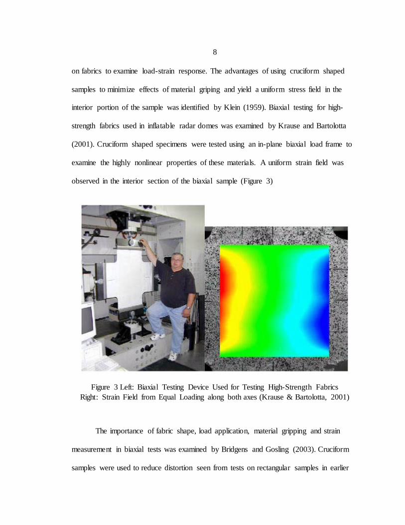
interior portion of the sample was identified by Klein (1959). Biaxial testing for high-
strength fabrics used in inflatable radar domes was examined by Krause and Bartolotta
(2001). Cruciform shaped specimens were tested using an in-plane biaxial load frame to
examine the highly nonlinear properties of these materials. A uniform strain field was
observed in the interior section of the biaxial sample (Figure 3)
Figure 3 Left: Biaxial Testing Device Used for Testing High-Strength Fabrics
Right: Strain Field from Equal Loading along both axes (Krause & Bartolotta, 2001)
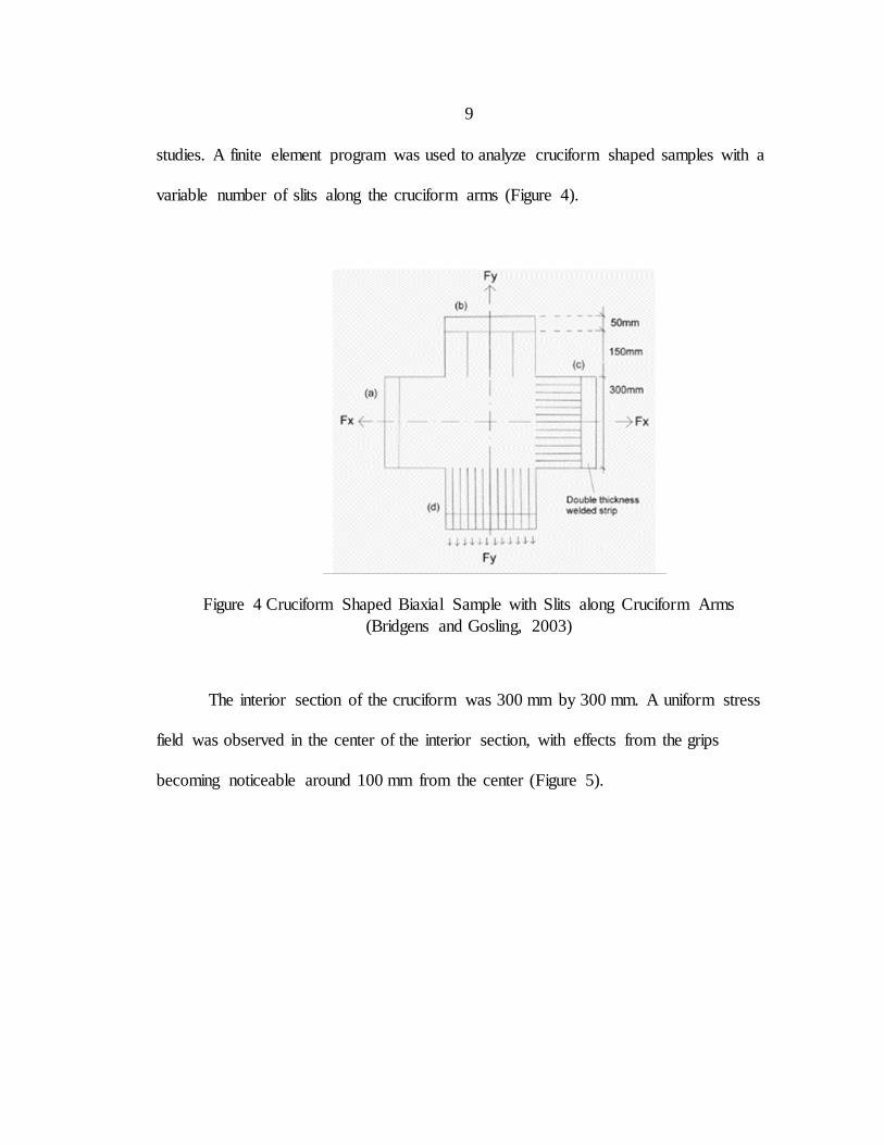
The importance of fabric shape, load application, material gripping and strain
measurement in biaxial tests was examined by Bridgens and Gosling (2003). Cruciform
samples were used to reduce distortion seen from tests on rectangular samples in earlier
9
studies. A finite element program was used to analyze cruciform shaped samples with a
variable number of slits along the cruciform arms (Figure 4).
Figure 4 Cruciform Shaped Biaxial Sample with Slits along Cruciform Arms
(Bridgens and Gosling, 2003)
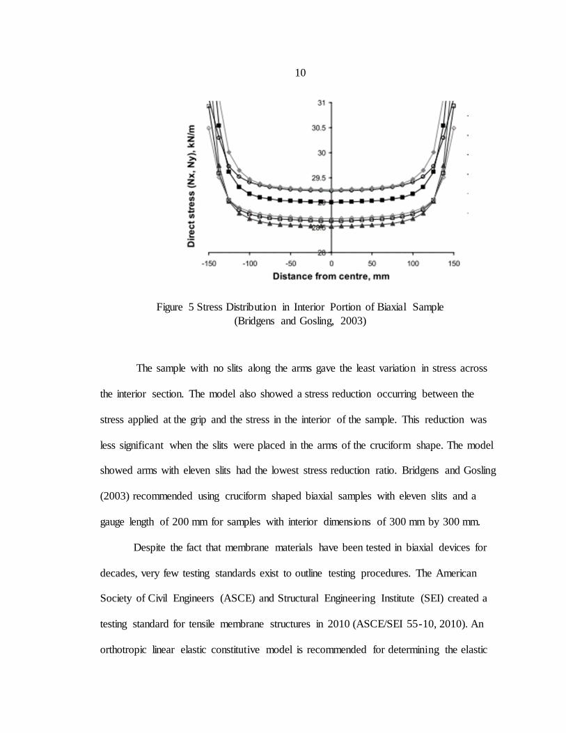
The interior section of the cruciform was 300 mm by 300 mm. A uniform stress
field was observed in the center of the interior section, with effects from the grips
becoming noticeable around 100 mm from the center (Figure 5).
10
Figure 5 Stress Distribution in Interior Portion of Biaxial Sample
(Bridgens and Gosling, 2003)
The sample with no slits along the arms gave the least variation in stress across
the interior section. The model also showed a stress reduction occurring between the
stress applied at the grip and the stress in the interior of the sample. This reduction was
less significant when the slits were placed in the arms of the cruciform shape. The model
showed arms with eleven slits had the lowest stress reduction ratio. Bridgens and Gosling
(2003) recommended using cruciform shaped biaxial samples with eleven slits and a
gauge length of 200 mm for samples with interior dimensions of 300 mm by 300 mm.
Despite the fact that membrane materials have been tested in biaxial devices for
decades, very few testing standards exist to outline testing procedures. The American
Society of Civil Engineers (ASCE) and Structural Engineering Institute (SEI) created a
testing standard for tensile membrane structures in 2010 (ASCE/SEI 55-10, 2010). An
orthotropic linear elastic constitutive model is recommended for determining the elastic
11
constants of membrane materials from biaxial tension tests on cruciform shaped samples
(ASCE/SEI 55-10, 2010). In order to solve for the elastic constants from measured stress
and strain data, the least squares method is recommended (ASCE/SEI 55-10, 2010). The
Membrane Structures Association of Japan created a Testing Method for Elastic
Constants of Membrane Materials (MSAJ, 1995) that is referenced as an outline in many
biaxial testing studies that proceeded it. The testing standard outlines a detailed testing
procedure including testing device specifications, test specimen specifications, test
procedures and methods for calculating the elastic constants of materials tested. The
Japanese standard recommends a biaxial testing device that is capable of applying loads
simultaneously in perpendicular directions such that the location of the center point of the
cruciform shaped specimen remains constant (MSAJ, 1995). The recommend test
specimen size is outlined in
. The recommended distance between initial standard points for measurement of
displacement was between 20 and 80 mm or at least 10 crossing yarns for a range of
strain measurement of -10 % to 20 %.
12
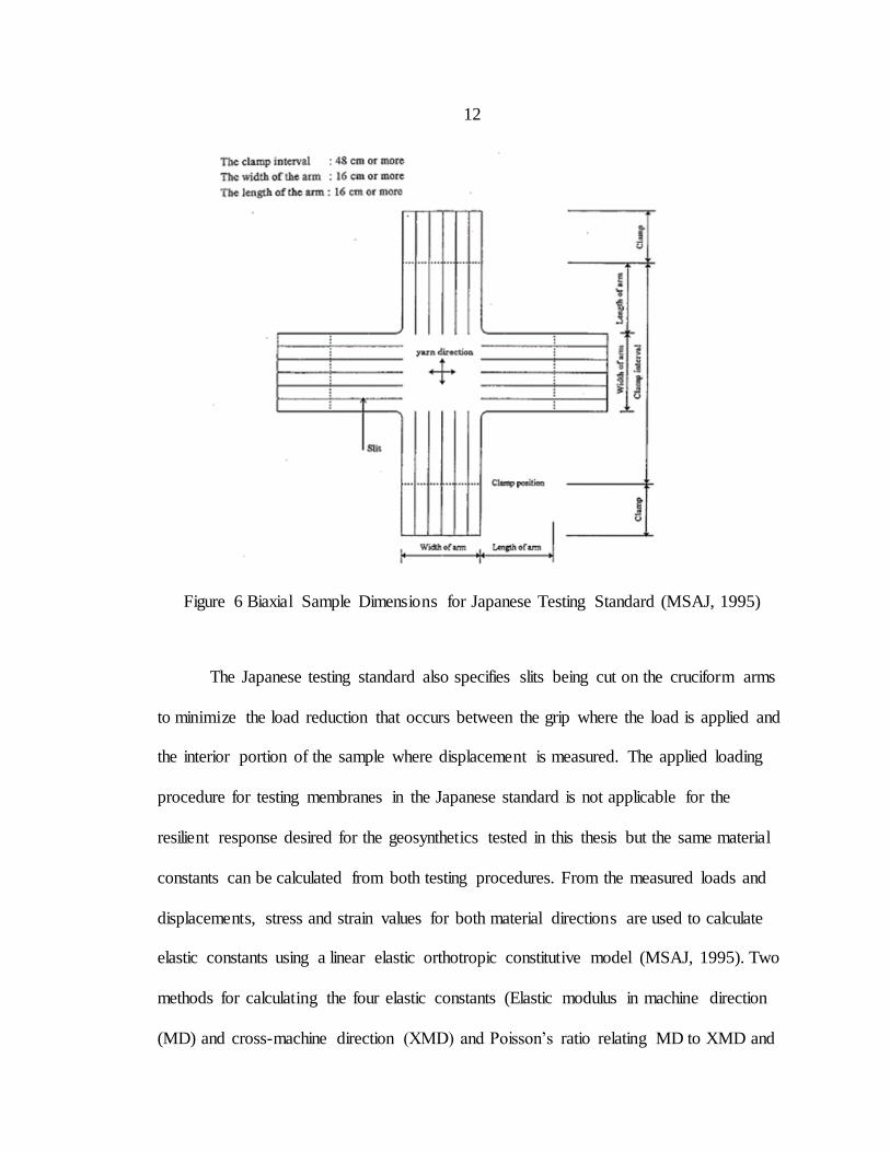
Figure 6 Biaxial Sample Dimensions for Japanese Testing Standard (MSAJ, 1995)
The Japanese testing standard also specifies slits being cut on the cruciform arms
to minimize the load reduction that occurs between the grip where the load is applied and
the interior portion of the sample where displacement is measured. The applied loading
procedure for testing membranes in the Japanese standard is not applicable for the
resilient response desired for the geosynthetics tested in this thesis but the same material
constants can be calculated from both testing procedures. From the measured loads and
displacements, stress and strain values for both material directions are used to calculate
elastic constants using a linear elastic orthotropic constitutive model (MSAJ, 1995). Two
methods for calculating the four elastic constants (Elastic modulus in machine direction
(MD) and cross-machine direction (XMD) and Poisson’s ratio relating MD to XMD and

13
XMD to MD directions) are used in the Japanese testing standard. The first method is a
Least-Squares Method that can be used to minimize the stress or strain terms of
governing equations (see Chapter Three of Thesis) using multiple load ratios. The other
suggested method is the Best Approximation Method or minimax method. Both methods
will be discussed further in proceeding sections of this thesis. Multiple tests and load
ratios are needed to calculate the elastic constants since only three independent equations
are available to calculate four unknowns for the selected linear elastic orthotropic model.
A number of testing programs and studies have been performed on structural
membranes in order to determine their elastic constants from biaxial laboratory testing.
The Japanese testing standard was referenced in a significant number of studies as an
outline for the testing procedure and a guide for calculating elastic constants. Bridgens
and Gosling (2010) examined the Japanese testing standard in detail. In this paper,
different methods for calculating elastic constants from biaxial tests performed on a
Ferrari 1202 PVC-polyester membrane were examined. The Japanese testing standard
outlines a procedure with multiple load ratios applied to the same material over the
course of one test. The load ratios are defined as the ratio of the load applied in each
perpendicular direction of a biaxial tension test. If equal load is applied in both directions,
the load ratio is 1:1. In the Japanese testing standard, load ratios of 0:1 and 1:0 are
specified in the testing procedure. The Japanese testing standard recommends not using
data in the direction of zero load for calculation of elastic constants. Bridgens and
Gosling (2010) examined differences in elastic constants when the data from these load
ratios was included. The Japanese testing standard uses an equation to relate Poisson’s
14
ratio in both directions referred to as the reciprocal constraint (ν12 ∗ E2 = ν21 ∗ E1 ).
Bridgens and Gosling (2010) examined the difference in elastic constants when this
equation was not used.
When coated woven fabrics used for structural membranes are subjected to high
loads over sustained periods of time, they develop some residual strain due to creep. In
the Japanese testing standard nothing is done to account for this residual strain in the
material so Bridgens and Gosling (2010) also examined the effect of removing this strain
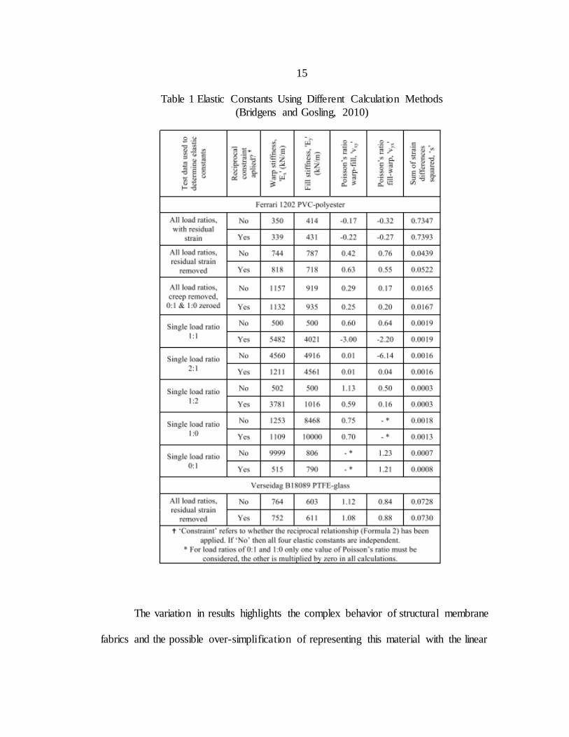
from their data. Significant variation in values of the elastic constants calculated was
observed between the different analysis approaches examined by Bridgens and Gosling
(2010). The results are shown in Table 1.
15
Table 1 Elastic Constants Using Different Calculation Methods
(Bridgens and Gosling, 2010)
The variation in results highlights the complex behavior of structural membrane
fabrics and the possible over-simplification of representing this material with the linear

16
elastic orthotropic model. Bridgens and Gosling (2010) concluded that use of the
reciprocal constraint had only a small effect on the calculated values for elastic constants
in comparison to the effect of removing residual strain. The removal of residual strain
was discussed in more detail by Bridgens and Gosling (2004). Beccarelli (2015) also
referenced the Japanese testing standard for calculating elastic constants from biaxial
tension tests. Craenenbroeck et al. (2015) used the testing procedure outlined in the
Japanese standard as well as variations of this procedure to calculate elastic constants for
structural membranes. It was found that when a loading protocol that mimicked field-
loading conditions for membranes was used instead of the standard protocol, a variation
in elastic constants occurred (Craenenbroeck et al., 2015).
The in-plane biaxial tests on structural membranes provided useful information
regarding biaxial testing devices, biaxial sample size/setup and use of stress and strain
data to calculate elastic constants with an orthotropic linear elastic constitutive model.
The specifics about loading procedure effects on elastic constants and membrane
behavior in general are slightly less applicable since a significantly different testing
procedure was used on significantly different materials for this thesis.
Biaxial Testing of Geosynthetics
The three most notable biaxial tests on geosynthetics have been conducted by
Kupec and McGown (2004), McGown et al. (2004) and Hangen et al. (2008). All three of
these studies were performed on biaxial geogrids.
17
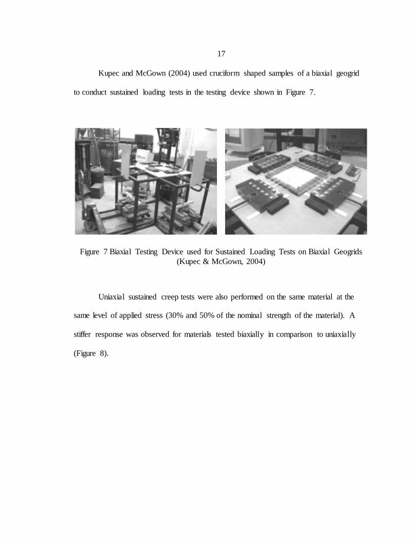
Kupec and McGown (2004) used cruciform shaped samples of a biaxial geogrid
to conduct sustained loading tests in the testing device shown in Figure 7.
Figure 7 Biaxial Testing Device used for Sustained Loading Tests on Biaxial Geogrids
(Kupec & McGown, 2004)
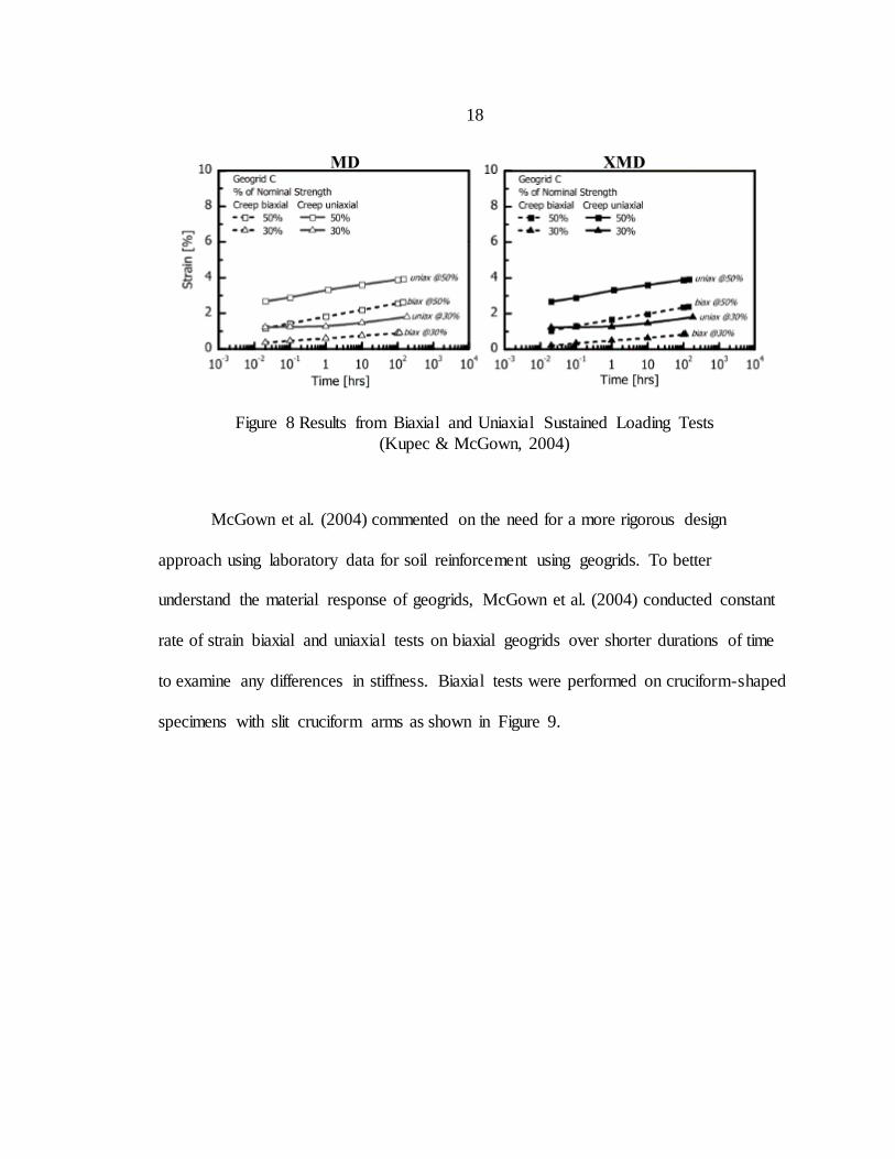
Uniaxial sustained creep tests were also performed on the same material at the
same level of applied stress (30% and 50% of the nominal strength of the material). A
stiffer response was observed for materials tested biaxially in comparison to uniaxially
(Figure 8).
18
Figure 8 Results from Biaxial and Uniaxial Sustained Loading Tests
(Kupec & McGown, 2004)
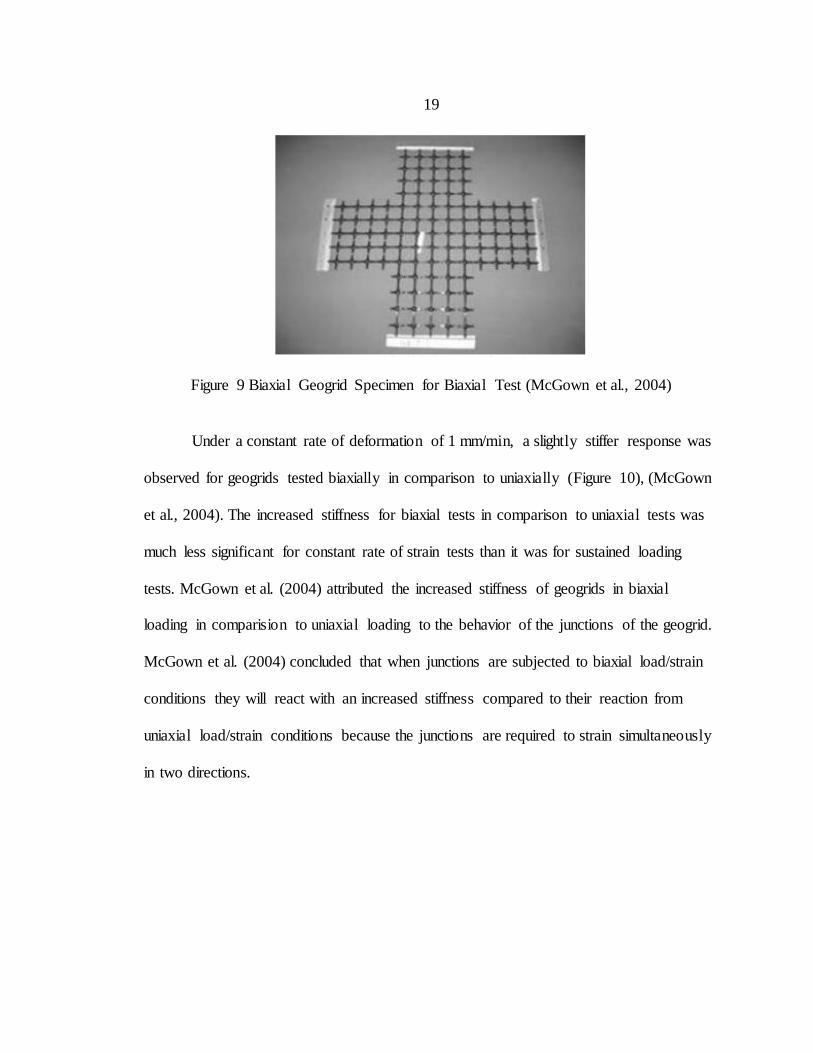
McGown et al. (2004) commented on the need for a more rigorous design
approach using laboratory data for soil reinforcement using geogrids. To better
understand the material response of geogrids, McGown et al. (2004) conducted constant
rate of strain biaxial and uniaxial tests on biaxial geogrids over shorter durations of time
to examine any differences in stiffness. Biaxial tests were performed on cruciform-shaped
specimens with slit cruciform arms as shown in Figure 9.
19
Figure 9 Biaxial Geogrid Specimen for Biaxial Test (McGown et al., 2004)
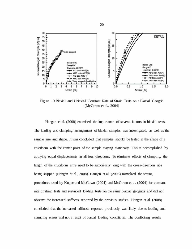
Under a constant rate of deformation of 1 mm/min, a slightly stiffer response was
observed for geogrids tested biaxially in comparison to uniaxially (Figure 10), (McGown
et al., 2004). The increased stiffness for biaxial tests in comparison to uniaxial tests was
much less significant for constant rate of strain tests than it was for sustained loading
tests. McGown et al. (2004) attributed the increased stiffness of geogrids in biaxial
loading in comparision to uniaxial loading to the behavior of the junctions of the geogrid.
McGown et al. (2004) concluded that when junctions are subjected to biaxial load/strain
conditions they will react with an increased stiffness compared to their reaction from
uniaxial load/strain conditions because the junctions are required to strain simultaneously
in two directions.
20
Figure 10 Biaxial and Uniaxial Constant Rate of Strain Tests on a Biaxial Geogrid
(McGown et al., 2004)
Hangen et al. (2008) examined the importance of several factors in biaxial tests.
The loading and clamping arrangement of biaxial samples was investigated, as well as the
sample size and shape. It was concluded that samples should be tested in the shape of a
cruciform with the center point of the sample staying stationary. This is accomplished by
applying equal displacements in all four directions. To eliminate effects of clamping, the
length of the cruciform arms need to be sufficiently long with the cross-direction ribs
being snipped (Hangen et al., 2008). Hangen et al. (2008) mimicked the testing
procedures used by Kupec and McGown (2004) and McGown et al. (2004) for constant
rate of strain tests and sustained loading tests on the same biaxial geogrids and did not
observe the increased stiffness reported by the previous studies. Hangen et al. (2008)
concluded that the increased stiffness reported previously was likely due to loading and
clamping errors and not a result of biaxial loading conditions. The conflicting results
21
reported by Hangen (2008) and McGown et al. (2004) and Kupec and McGown (2004)
highlight the need for additional biaxial testing.
Synthesis of Literature Review
The literature examined for this thesis was helpful for the process of creating a
biaxial testing procedure for geosynthetics that could be used to simulate a resilient
response of geosynthetics subjected to relatively low biaxial loads. The procedure for
Determining Small-Strain Tensile Properties of Geogrids and Geotextiles by In-Air
Cyclic Tension Tests (ASTM D7556) was most applicable for the desired resilient
response of geosynthetics. A form of this procedure was adopted using other information
regarding biaxial testing devices, sample specifications and calculation of elastic
constants for biaxial samples of geosynthetics using in-plane biaxial tension tests.
Limitations of the biaxial testing device available for this thesis also were examined and
modifications were made to the testing procedure and data analysis to best utilize the
testing equipment and data collection systems available.
22
CHAPTER THREE
THEORY
Constitutive Equations
An orthotropic linear elastic model was used to describe the behavior of geosynthetics
subjected to biaxial tension tests. For the entirety of this thesis, stress will be expressed as
force per length, as dividing by the thickness of the geosynthetic to get the true units of
stress is not commonly done for geosynthetics. The inputs for the constitutive equations
are the stress and strain measured in both principle directions of the material. The
constitutive equations are used to calculate four elastic constants for the material. The
elastic constants calculated are the modulus of elasticity in both material directions and
Poisson’s ratio in both material directions. Only three of the elastic constants are
independent when the reciprocal constraint is applied (Equation (9)). The orthotropic
linear elastic constants were calculated using the general relationship between stress and
strain shown in Equation (1). For biaxial loading, the general form of the equation can be
reduced to Equation (2) because the material is in a state of plane stress. A further
simplification resulting in Equation (3) can be made assuming biaxial samples are in a
state of pure tension. Equation (3) was used for calculation of the three independent
elastic constants for geosynthetics. The three independent elastic constants that were
solved for are the modulus of elasticity in both directions (E1 and E2) and Poisson’s Ratio
(ν12). These elastic constants appear in terms in the stiffness matrix, which are defined in
23
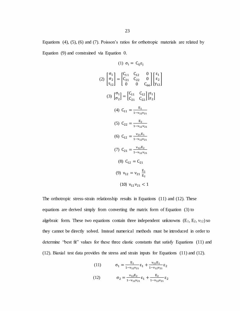
Equations (4), (5), (6) and (7). Poisson’s ratios for orthotropic materials are related by
Equation (9) and constrained via Equation 0.
(1) σi = Cijεj
(2) [
σ1
σ2
τ12
] = [C11 C12 0C21 C22 00 0 C66
] [
ε1ε2
γ12
]
(3) [σ1
σ2] = [
C11 C12
C21 C22] [
ε1ε2
]
(4) C11 =E1
1−ν12ν21
(5) C22 =E2
1−ν12ν21
(6) C12 =ν21E1
1−ν12ν21
(7) C21 =ν12E2
1−ν12ν21
(8) C12 = C21
(9) ν12 = ν21 E1
E2
(10) ν12ν21 < 1
The orthotropic stress-strain relationship results in Equations (11) and (12). These
equations are derived simply from converting the matrix form of Equation (3) to
algebraic form. These two equations contain three independent unknowns (E1, E2, ν12) so
they cannot be directly solved. Instead numerical methods must be introduced in order to
determine “best fit” values for these three elastic constants that satisfy Equations (11) and
(12). Biaxial test data provides the stress and strain inputs for Equations (11) and (12).
(11) σ1 =E1
1−ν12ν21ε1 +
ν21E1
1−ν12ν21ε2
(12) σ2 =ν12E2
1−ν12ν21ε1 +
E2
1−ν12ν21ε2
24
Numerical Methods
The constitutive equations used to solve for the elastic constants results in a
system of equations that is indeterminate for a single biaxial test since only Equations
(11) and (12) are available for solving three independent elastic constants. To solve for
the elastic constants, additional tests must be conducted at varied load ratios. This allows
additional equations to be generated in the form of equations (11) and (12) with different
values for stress and strain inputs (MSAJ, 1995). Once additional load ratios are used,
numerical methods can be implemented to determine what set of elastic constants best
fits the measured stress and strain responses for multiple load ratios. The most common
approach for solving this system of equations is a least squares approximation. The least
squares approach is outlined in the Japanese testing standard and has been implemented
for numerous studies using biaxial tension tests to calculate elastic constants for
membrane materials.
The least squares method was examined in a more general format to confirm the
method outlined in the Japanese testing standard was applicable. The least squares
technique is useful when there is a positive correlation between x and y that cannot
accurately be predicted by polynomial interpolation or other approximation techniques
(Chapra, Canale, 1998). In the case of biaxial tension tests, there is a positive relationship
between measured stress and strain values that can be related by the elastic constants in
the orthotropic linear elastic model. A least squares regression uses an approximating
function that does not necessarily pass through all data points but generally predicts the
trend of the data (Chapra, Canale, 1998). In order to provide a unique approximation that
25
“best” fits the given data, a minimization of the sum of the squares of the residuals is
used as shown in Equation (13) (Chapra, Canale, 1998).
(13) S = ∑( yi,measured − yi,model)2
A general least squares approach for a given data set tries to approximate the data using
an approximating function in the form of Equation (14). The approximating function for
general leas squares is required to have a linear dependence on its parameters (a1, a2…an)
(Chapra, Canale, 1998). The least squares approximating function (Equation (14))
approximates function values (y) using the parameters (a1, a2,…,an) and basis functions
(z1, z2,…,zm), where the parameters are the unknowns and the basis functions are a
function of the x values.
Given Data: (xi , yi) for i = 1, … , n
(14) Approximating Function:f(x) = a1z1 + a2z2 + ⋯+ amzm
As mentioned previously, the goal of the approximating function is to minimize the error
(residuals) between the data values for y and the approximated values or f (x) values. To
minimize the residuals, a function is defined as follows (Chapra, Canale, 1998),
(15) Sr = ∑ (yi− f(xi))
2ni=1
To solve for the parameters in the approximating function (a1, a2 and an) the partial
derivatives of Sr with respect to a1, a2 and an are set equal to zero (Chapra, Canale, 1998).
(16) ∂Sr
∂a1=
∂Sr
∂a2=
∂Sr
∂an= 0
The general least squares approach can be applied to stress and strain data from biaxial
tension tests to solve for the elastic constants in an orthotropic linear elastic constitutive
26
model. The least squares approach can be used to minimize the residuals in the stress
term or in the strain term for a given data set from biaxial tension tests. The method to
minimize the stress term, as shown in the Japanese Testing Standard, uses Equations (11)
and (12), which are rewritten using equations (4) -(7) to be in a linear form as required
for general least squares. The stress term for each direction (σ1, σ2) are written as a
function of the strain terms (ε1, ε2) and parameters (C11 ,C12 , C22) in the same format as
Equation (14).
(17) σ1 = C11ε1 + C12ε2
(18) σ2 = C21ε1 + C22ε2
The following equation is written in the form of Equation (15) (MSAJ, 1995) using the
measured values of stress and strain from a biaxial test.
(19) S = ∑{(C11ε1 + C12ε2 − σ1)2 + (C21ε1 + C22ε2 − σ2)
2}
The partial derivatives of S with respect to the parameters in the approximating function
(C11 , C12, C22) are set equal to zero according to Equation (16) (MSAJ, 1995).
(20) ∂S
∂C11=
∂S
∂C22=
∂S
∂C12= 0
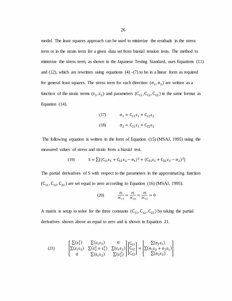
A matrix is setup to solve for the three constants (C11, C12 , C22) by taking the partial
derivatives shown above as equal to zero and is shown in Equation 21.
(21) [
∑(ε12) ∑(ε1ε2) 0
∑(ε1ε2) ∑(ε22 + ε1
2) ∑(ε1ε2)
0 ∑(ε1ε2) ∑(ε22)
] [C11
C12
C22
] = [
∑(σ1ε1)
∑(σ1ε2 + σ2ε1)∑(σ2ε2)
]
27
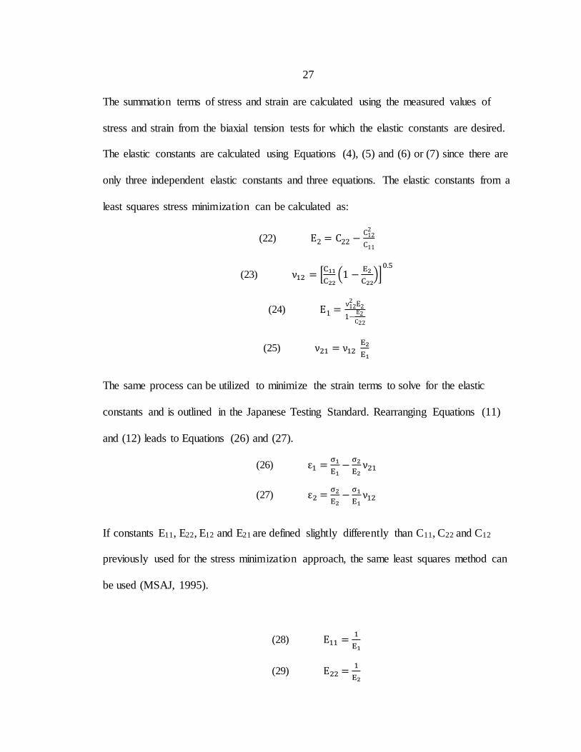
The summation terms of stress and strain are calculated using the measured values of
stress and strain from the biaxial tension tests for which the elastic constants are desired.
The elastic constants are calculated using Equations (4), (5) and (6) or (7) since there are
only three independent elastic constants and three equations. The elastic constants from a
least squares stress minimization can be calculated as:
(22) E2 = C22 −C122
C11
(23) ν12 = [C11
C22(1 −
E2
C22)]
0.5
(24) E1 =ν122 E2
1−E2C22
(25) ν21 = ν12 E2
E1
The same process can be utilized to minimize the strain terms to solve for the elastic
constants and is outlined in the Japanese Testing Standard. Rearranging Equations (11)
and (12) leads to Equations (26) and (27).
(26) ε1 =σ1
E1−
σ2
E2ν21
(27) ε2 =σ2
E2−
σ1
E1ν12
If constants E11, E22, E12 and E21 are defined slightly differently than C11, C22 and C12
previously used for the stress minimization approach, the same least squares method can
be used (MSAJ, 1995).
(28) E11 =1
E1
(29) E22 =1
E2
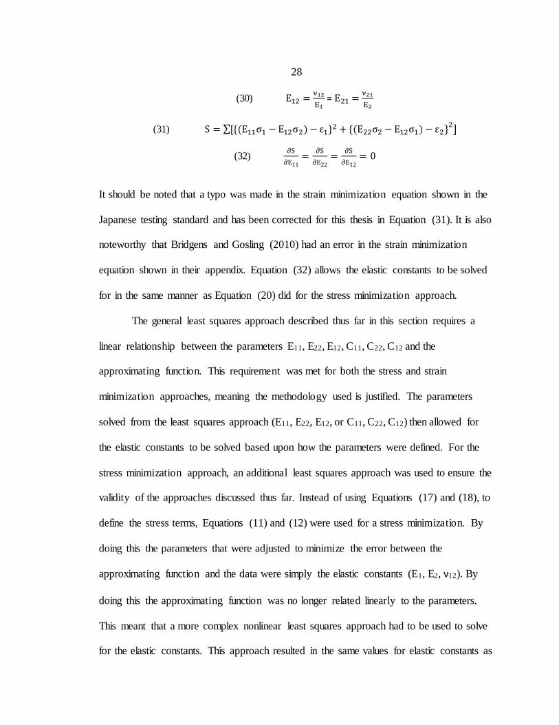
28
(30) E12 =ν12
E1 = E21 =
ν21
E2
(31) S = ∑[{(E11σ1 − E12σ2) − ε1}2 + {(E22σ2 − E12σ1) − ε2}
2]
(32) ∂S
∂E11=
∂S
∂E22=
∂S
∂E12= 0
It should be noted that a typo was made in the strain minimization equation shown in the
Japanese testing standard and has been corrected for this thesis in Equation (31). It is also
noteworthy that Bridgens and Gosling (2010) had an error in the strain minimization
equation shown in their appendix. Equation (32) allows the elastic constants to be solved
for in the same manner as Equation (20) did for the stress minimization approach.
The general least squares approach described thus far in this section requires a
linear relationship between the parameters E11, E22, E12, C11, C22, C12 and the
approximating function. This requirement was met for both the stress and strain
minimization approaches, meaning the methodology used is justified. The parameters
solved from the least squares approach (E11, E22, E12, or C11, C22, C12) then allowed for
the elastic constants to be solved based upon how the parameters were defined. For the
stress minimization approach, an additional least squares approach was used to ensure the
validity of the approaches discussed thus far. Instead of using Equations (17) and (18), to
define the stress terms, Equations (11) and (12) were used for a stress minimization. By
doing this the parameters that were adjusted to minimize the error between the
approximating function and the data were simply the elastic constants (E1, E2, ν12). By
doing this the approximating function was no longer related linearly to the parameters.
This meant that a more complex nonlinear least squares approach had to be used to solve
for the elastic constants. This approach resulted in the same values for elastic constants as
29
the linear least squares approach for a given data set of stress and strain values. The
nonlinear approach is shown in Appendix A.
Several other methods for calculating the elastic constants from biaxial tension
tests are presented in MSAJ (1995) and Bridgens and Gosling (2004). The Japanese
testing standard also mentions the best approximation or minimax method for calculating
elastic constants. The elastic constants calculated using this method showed no notable
difference between the least squares technique (MSAJ, 1995). The best approximation
method was much more difficult to understand and apply and was not used in any
literature encountered for biaxial tension tests. For these reasons, this method was not
implemented for this research. The third method presented in the Japanese testing
standard is a multi-step linear approximation of material constants on the nonlinear
extension curves. This method is recommended for use when load-extension curves are
clearly not well represented by a linear line. For this thesis, the stress and strain data used
was over small regions of strain such that load-extension curves were well represented
with linear lines, meaning this approach was not necessary. Bridgens and Gosling (2004)
and Bridgens and Gosling (2010) examine some modifications to the Japanese testing
standard methods for calculating elastic constants for membrane materials. These
modifications are discussed in the literature review section of this thesis and are not
applicable for the analysis of geosynthetics in this thesis.
The solver in Microsoft Excel was also experimented with for calculating the
elastic constants. The solver used in Microsoft Excel uses the Generalized Reduced
Gradient (GRG) nonlinear algorithm. Initially this approach was desired because of its
30
simplicity and ability to produce a unique value for elastic constants using only one value
of stress and strain in each material direction. After further analysis of this approach, it
was seen to be inadequate because of the strong dependence on initial guess values used
for elastic constants. The solver will converge on a possible combination of elastic
constants near the guessed values that satisfy Equations 11 and 12 with some amount of
error. This solution for the elastic constants is not a unique or a “best” fit solution. For
these reasons, the least squares approaches were used for solving for the elastic constants
of geosynthetics from biaxial tension tests.
31
CHAPTER FOUR
TESTING PROCEDURE DEVELOPMENT
Testing Procedure Objective
The goal of this research project was to quantitatively describe the mechanical
resilient behavior of geosynthetics subjected to repetitive loading in multiple directions
that simulates field loading conditions in applications such as reinforced pavements. In
repetitive loading applications such as roads, it is expected that geosynthetics experience
both cyclic creep and cyclic stress relaxation. In ASTM D7556, only cyclic stress
relaxation is used to create a resilient response in geosynthetics. It was hypothesized that
the resilient response seen after cyclic loading could also be achieved from sustained
monotonic loading. It was thought that if a material was held at a constant value of strain
and the load was allowed to relax as it does in cyclic stress relaxation, that this would
create the same resilient response. It was also hypothesized that subjecting a material to
stress relaxation and/or creep would both simulate the same resilient response. The time
necessary for a geosynthetic to exhibit “resilient” behavior was also of interest for
developing a biaxial tension test procedure for geosynthetics that simulates a resilient
response.
Initially, it was desired to use the biaxial device to examine resilient response
under the types of loads discussed above. The ability to control load and strain with the
biaxial testing device was insufficient to carry out precise and repeatable cyclic tests. It
was also discovered that the interior portion of the biaxial sample experienced a
32
combination of mostly stress relaxation with some creep when it was held at a constant
displacement. It was not possible to limit the loading to only stress relaxation or only
creep. Due to these limitations with the biaxial testing device available for this project,
uniaxial wide-width tension tests were performed to examine differences in material
resilient response from four types of loading, namely cyclic stress relaxation, monotonic
stress relaxation, cyclic stress creep and monotonic stress creep.
Uniaxial Testing Overview
Uniaxial wide width tensile tests were performed using several modes of loading
to establish a testing procedure using the biaxial device. (You have probably noticed that
I have changed a lot of sentences like this where you start the sentence with an outcome,
pause with a comma, then describe how you got to the outcome. I prefer to write the
sentence in the order of the events that took place. I do not know if one is more correct
than the other. I think that the sequential approach is more technically clean and to the
point.) The goal of the uniaxial testing program was to examine differences in material
response when a material was allowed to relax or creep by being subjected to cyclic
loading or monotonic loading. The conclusions of the uniaxial tests were critical for
showing that the biaxial testing device was capable of producing data that was
representative of field loading conditions and could be used for determining elastic
constants. Wide width tensile tests were performed using four different methods. Tests
were performed as cyclic stress relaxation tests, cyclic creep, monotonic stress relaxation
and monotonic creep tests. These four types of tests were performed using ASTM D7556
33
as a guideline when applicable. The widths and gauge lengths used for the uniaxial wide
width tests on both the woven geotextile and biaxial geogrid were approximately 200
millimeters. The time necessary for the material to relax/creep was also examined using
wide-width tensile tests.
Uniaxial Testing Device
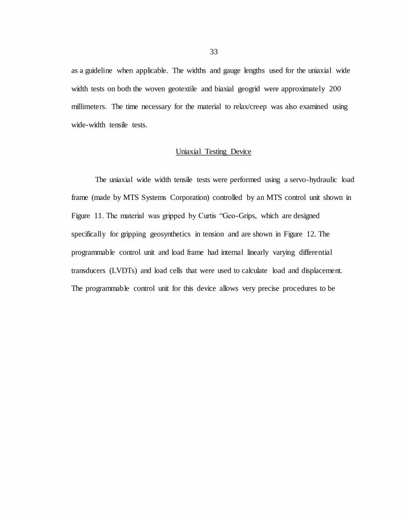
The uniaxial wide width tensile tests were performed using a servo-hydraulic load
frame (made by MTS Systems Corporation) controlled by an MTS control unit shown in
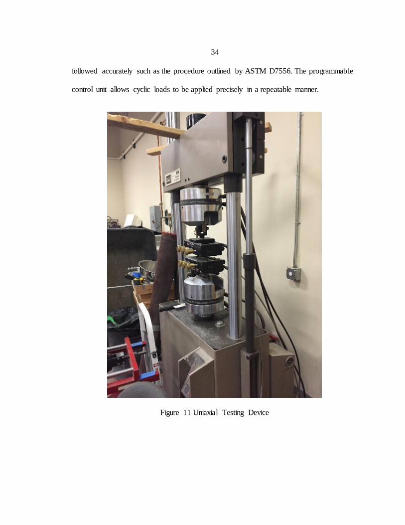
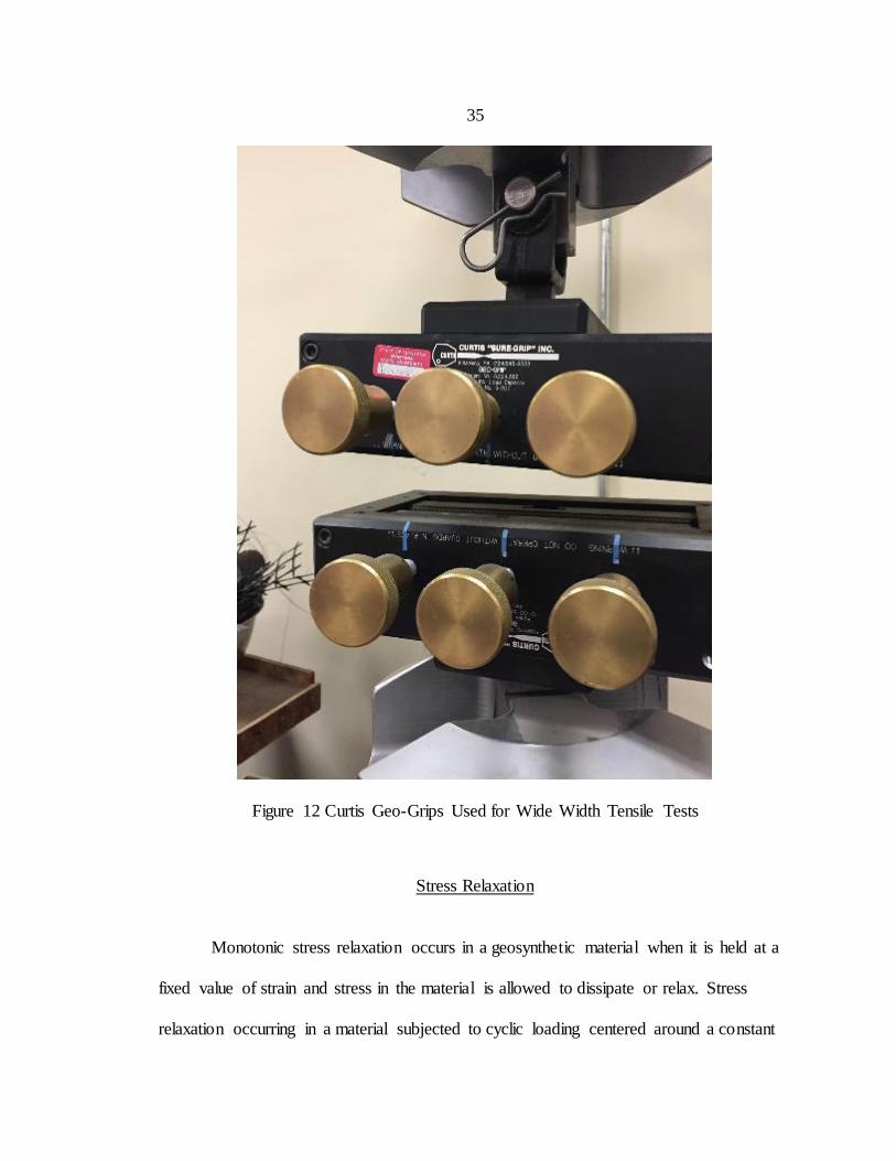
Figure 11. The material was gripped by Curtis “Geo-Grips, which are designed
specifically for gripping geosynthetics in tension and are shown in Figure 12. The
programmable control unit and load frame had internal linearly varying differential
transducers (LVDTs) and load cells that were used to calculate load and displacement.
The programmable control unit for this device allows very precise procedures to be
34
followed accurately such as the procedure outlined by ASTM D7556. The programmable
control unit allows cyclic loads to be applied precisely in a repeatable manner.
Figure 11 Uniaxial Testing Device
35
Figure 12 Curtis Geo-Grips Used for Wide Width Tensile Tests
Stress Relaxation
Monotonic stress relaxation occurs in a geosynthetic material when it is held at a
fixed value of strain and stress in the material is allowed to dissipate or relax. Stress
relaxation occurring in a material subjected to cyclic loading centered around a constant
36
value of strain is referred to as cyclic stress relaxation. Cyclic stress relaxation test
procedures and methodology used for determination of resilient modulus values are
outlined in ASTM D7556. No testing standards exist for sustained loading tests or
monotonic stress relaxation tests used for determination of resilient modulus. It was
hypothesized that monotonic stress relaxation tests and cyclic stress relaxation tests
would result in similar values of resilient modulus. This hypothesis was never tested in a
laboratory setting thus it was examined for this research.
Cyclic stress relaxation tests were performed on a biaxial geogrid and a woven
geotextile according to the procedure in ASTM D7556. This procedure involved loading
the material monotonically to 0.5 % strain, then applying 1000 cycles of load
corresponding to ±0.1 % strain. The material was next loaded monotonically to 1.0 %
strain then subjected to the same load cycles as at the previous level of permanent strain.
This process was repeated for permanent strain levels of 1.5, 2.0, 3.0 and 4.0 % strain.
Monotonic stress relaxation tests were performed on the same biaxial geogrid and
woven geotextile as cyclic stress relaxation tests. The procedure outlined above in ASTM
D7556 was adopted for monotonic stress relaxation tests except instead of applying 1000
cycles at each value of permanent strain, the strain was held constant for a predetermined
amount of time.
Creep under Sustained Load
Creep occurs in a geosynthetic material when it is subjected to a constant stress.
As with stress relaxation, creep can be achieved by applying cyclic and monotonic loads.
37
The resilient modulus in geosynthetics subjected to monotonic or cyclic creep has not
been studied previously and thus was also examined in a laboratory setting for this thesis.
Due to time constraints, the majority of uniaxial wide width tensile tests were performed
as stress relaxation tests. The results from creep tests were slightly less important because
of the small amount that occurs in the biaxial testing device as compared to stress
relaxation. It was also difficult to determine a procedure that would allow results to be
directly compared to stress relaxation data. This problem was especially pronounced for
cyclic creep tests because there is no guideline for what load should be cycled. Time
constraints on the project also limited the amount of creep tests that were performed.
Creep tests were performed using a procedure that was intended to match as
closely as possible the procedure used for stress relaxation tests. The material was
initially loaded monotonically to a permanent strain value of 0.5 % then allowed to creep
(either monotonically or by the application of load cycles). This process was continued
for permanent strain limits of 1.0, 1.5, 2.0, 3.0 and 4.0 % strain. The issue encountered in
this procedure was that the programmable uniaxial testing device procedures must either
be displacement or load controlled for the entirety of a procedure. Precise permanent
strain limits were desired for comparison to stress relaxation tests, but since load must be
held constant for creep tests, this presented some procedural difficulties. This along with
the desire to examine the effects of the length of time a material is allowed to creep or
relax led to the development of a slightly different procedure for creep tests. The
procedure that followed was to conduct creep tests starting at a single value of 4.0 %
permanent strain. The material was loaded to this value of permanent strain and allowed
38
to creep for a period of 24 hours. Single cycles of load were applied at various times
throughout the 24-hour period so that a resilient modulus versus time relationship could
be developed.
Effect of Stress Relaxation and Creep Duration
The effect of the duration of time a geosynthetic was allowed to creep or relax on
the resilient modulus was of interest for developing a biaxial testing procedure. To
examine this effect, single stage (initially loaded monotonically to a permanent strain of
4.0 %) 24-hour tests were performed as described in the creep section. Stress relaxation
tests were performed in a similar manner, where the material was loaded monotonically
to a permanent strain value of 4.0 % then stress relaxation was induced either cyclically
or monotonically. The results of all uniaxial testing are presented in Chapter 5 of this
thesis. A summary of all uniaxial wide width tensile tests performed is shown below in
Table 2.
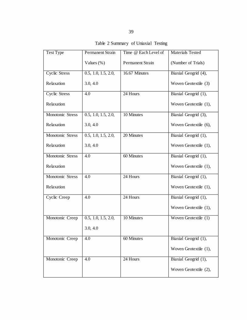
39
Table 2 Summary of Uniaxial Testing
Test Type Permanent Strain
Values (%)
Time @ Each Level of
Permanent Strain
Materials Tested
(Number of Trials)
Cyclic Stress
Relaxation
0.5, 1.0, 1.5, 2.0,
3.0, 4.0
16.67 Minutes Biaxial Geogrid (4),
Woven Geotextile (3)
Cyclic Stress
Relaxation
4.0 24 Hours Biaxial Geogrid (1),
Woven Geotextile (1),
Monotonic Stress
Relaxation
0.5, 1.0, 1.5, 2.0,
3.0, 4.0
10 Minutes Biaxial Geogrid (3),
Woven Geotextile (6),
Monotonic Stress
Relaxation
0.5, 1.0, 1.5, 2.0,
3.0, 4.0
20 Minutes Biaxial Geogrid (1),
Woven Geotextile (1),
Monotonic Stress
Relaxation
4.0 60 Minutes Biaxial Geogrid (1),
Woven Geotextile (1),
Monotonic Stress
Relaxation
4.0 24 Hours Biaxial Geogrid (1),
Woven Geotextile (1),
Cyclic Creep 4.0 24 Hours Biaxial Geogrid (1),
Woven Geotextile (1),
Monotonic Creep 0.5, 1.0, 1.5, 2.0,
3.0, 4.0
10 Minutes Woven Geotextile (1)
Monotonic Creep 4.0 60 Minutes Biaxial Geogrid (1),
Woven Geotextile (1),
Monotonic Creep 4.0 24 Hours Biaxial Geogrid (1),
Woven Geotextile (2),
40
CHAPTER FIVE
UNIAXIAL TESTING RESULTS AND INTERPRETATION
Uniaxial Testing Results
As discussed in Chapter Four, uniaxial tests (wide width tensile tests) were
performed on a biaxial geogrid and a woven geotextile in their cross-machine direction.
Uniaxial tests were performed using multiple procedures for examination of different
effects as described in Chapter Four and summarized in Table 2. The raw data obtained
from uniaxial tests was displacement and load, which were used to calculate strain and
line load (stress) from the dimensions of the specimen tested. The stress vs. strain data
was used to calculate a modulus for a given level of permanent strain as the initial slope
of the stress vs. strain plot after stress relaxation or creep. The uniaxial modulus values at
a certain level of permanent strain could then be compared from different types of
loading to examine any differences.
Cyclic Stress Relaxation
Cyclic stress relaxation tests were performed according to ASTM D7556 as
described in Chapter Four. The cycles were performed at a rate of 1 hertz such that the
total cycle time for 1000 cycles at a given level of permanent strain was 16.67 minutes.
The load that was cycled corresponded to ±0.1 % strain. The results for a biaxial geogrid
and woven geotextile are shown below in Figure 13 and Figure 14.

41
Figure 13 Cyclic Stress Relaxation Test on a Biaxial Geogrid
Figure 14 Cyclic Stress Relaxation Test on Woven Geotextile
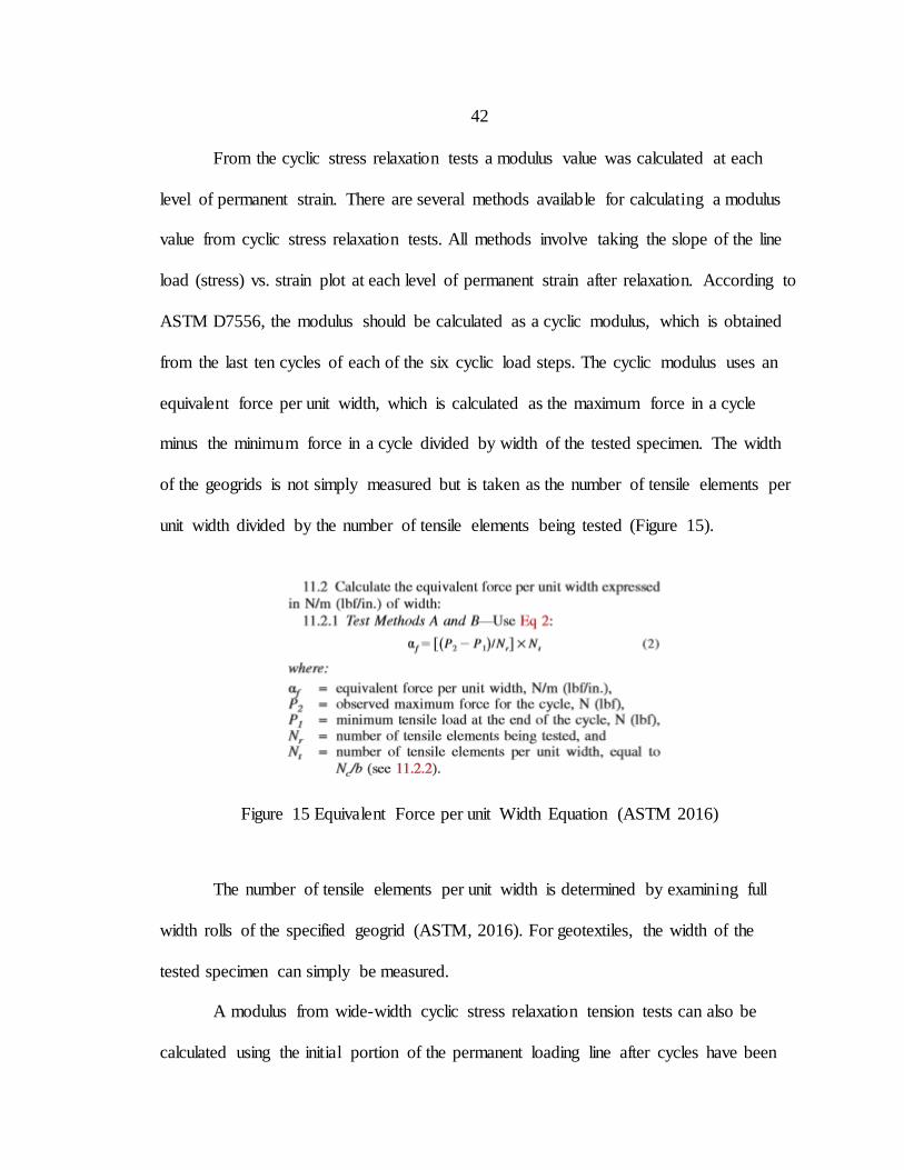
42
From the cyclic stress relaxation tests a modulus value was calculated at each
level of permanent strain. There are several methods available for calculating a modulus
value from cyclic stress relaxation tests. All methods involve taking the slope of the line
load (stress) vs. strain plot at each level of permanent strain after relaxation. According to
ASTM D7556, the modulus should be calculated as a cyclic modulus, which is obtained
from the last ten cycles of each of the six cyclic load steps. The cyclic modulus uses an
equivalent force per unit width, which is calculated as the maximum force in a cycle
minus the minimum force in a cycle divided by width of the tested specimen. The width
of the geogrids is not simply measured but is taken as the number of tensile elements per
unit width divided by the number of tensile elements being tested (Figure 15).
Figure 15 Equivalent Force per unit Width Equation (ASTM 2016)
The number of tensile elements per unit width is determined by examining full
width rolls of the specified geogrid (ASTM, 2016). For geotextiles, the width of the
tested specimen can simply be measured.
A modulus from wide-width cyclic stress relaxation tension tests can also be
calculated using the initial portion of the permanent loading line after cycles have been
43
applied. The modulus from the initial portion of the permanent loading can be calculated
as a secant modulus or using a linear approximation (best fit linear trendline). The secant
modulus and linear trendline modulus are calculated using the initial 0.2% strain of the
permanent loading stress-strain curve. The secant modulus was calculated using an
average of five points at the beginning and end of the 0.2% strain interval. The initial
reloading of geosynthetics after stress relaxation exhibits linear behavior, thus the three
methods mentioned for calculating the slope of the linear (modulus) should be equivalent.
The only reason for any differences would arise from the cyclic modulus being calculated
as the average slope of 10 cycles, while the secant and linear approximation are only
from the single permanent loading curve. Slight differences in value could also arise from
the material response not being perfectly linear or erroneous data points. Since the
modulus values from cyclic relaxation tests are meant to be comparable to modulus
values from monotonic tests, the modulus was only calculated using the initia l portion of
the permanent loading curve at each level of permanent strain after stress relaxation. The
modulus was calculated at each level of permanent strain after relaxation for all cyclic
stress relaxation trials from the initial 0.2 % strain of the permanent loading curve. The
modulus at each level of permanent strain for each trial is summarized in Table 3 and
Table 4 with an associated average, standard deviation and coefficient of variability for
both the biaxial geogrid and woven geotextile. The standard deviation and coefficie nt of
variability was calculated for tests that had multiple trials performed so that inherent
variability of identical tests could be compared to the variability between dissimilar tests
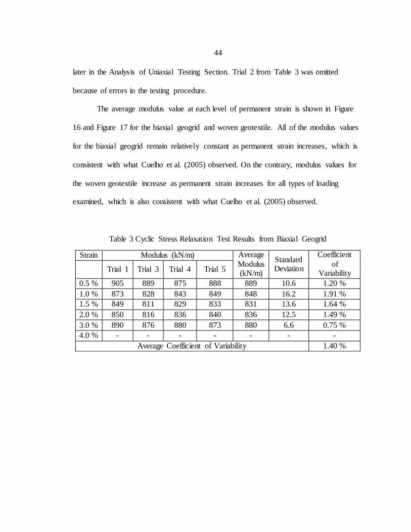
44
later in the Analysis of Uniaxial Testing Section. Trial 2 from Table 3 was omitted
because of errors in the testing procedure.
The average modulus value at each level of permanent strain is shown in Figure
16 and Figure 17 for the biaxial geogrid and woven geotextile. All of the modulus values
for the biaxial geogrid remain relatively constant as permanent strain increases, which is
consistent with what Cuelho et al. (2005) observed. On the contrary, modulus values for
the woven geotextile increase as permanent strain increases for all types of loading
examined, which is also consistent with what Cuelho et al. (2005) observed.
Table 3 Cyclic Stress Relaxation Test Results from Biaxial Geogrid
Strain Modulus (kN/m) Average
Modulus (kN/m)
Standard Deviation
Coefficient
of Variability
Trial 1 Trial 3 Trial 4 Trial 5
0.5 % 905 889 875 888 889 10.6 1.20 %
1.0 % 873 828 843 849 848 16.2 1.91 %
1.5 % 849 811 829 833 831 13.6 1.64 %
2.0 % 850 816 836 840 836 12.5 1.49 %
3.0 % 890 876 880 873 880 6.6 0.75 %
4.0 % - - - - - - -
Average Coefficient of Variability 1.40 %
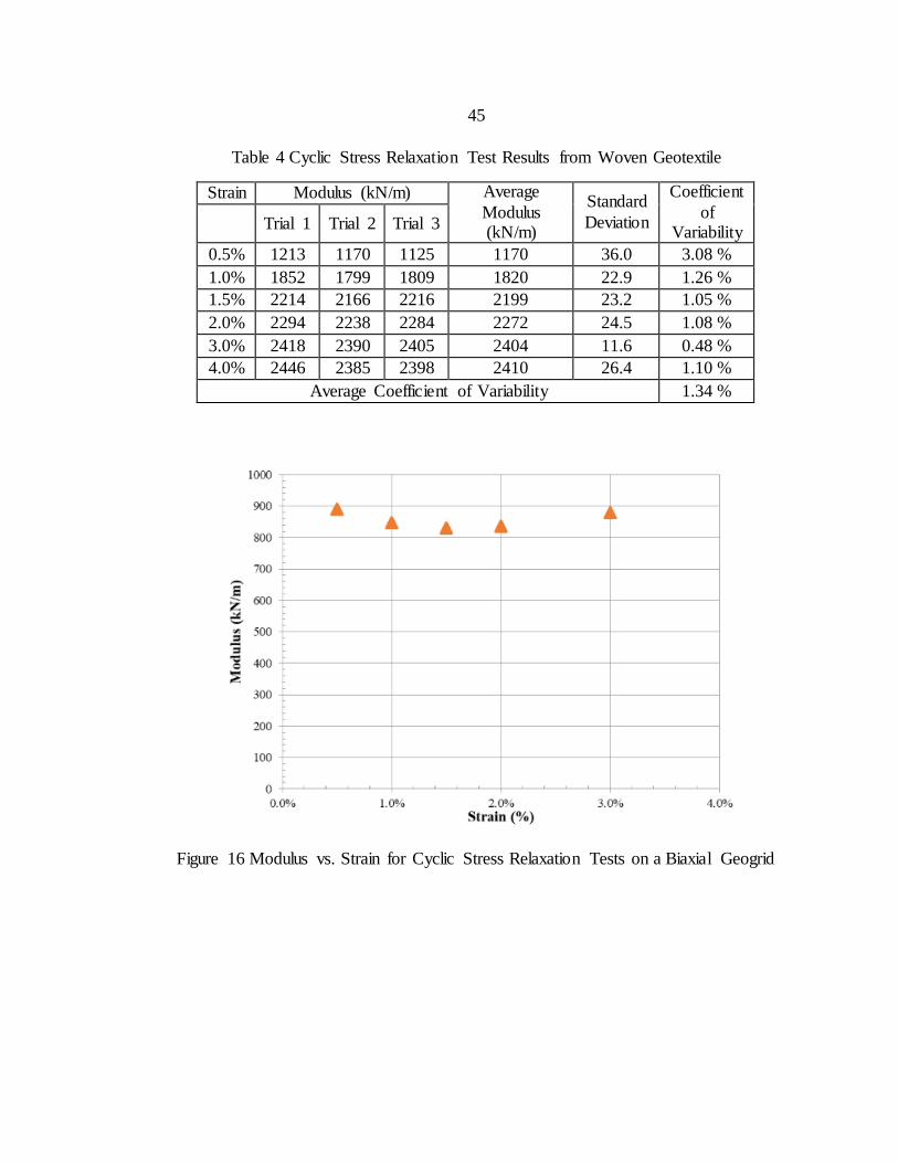
45
Table 4 Cyclic Stress Relaxation Test Results from Woven Geotextile
Strain Modulus (kN/m) Average
Modulus (kN/m)
Standard
Deviation
Coefficient
of Variability
Trial 1 Trial 2 Trial 3
0.5% 1213 1170 1125 1170 36.0 3.08 %
1.0% 1852 1799 1809 1820 22.9 1.26 %
1.5% 2214 2166 2216 2199 23.2 1.05 %
2.0% 2294 2238 2284 2272 24.5 1.08 %
3.0% 2418 2390 2405 2404 11.6 0.48 %
4.0% 2446 2385 2398 2410 26.4 1.10 %
Average Coefficient of Variability 1.34 %
Figure 16 Modulus vs. Strain for Cyclic Stress Relaxation Tests on a Biaxial Geogrid
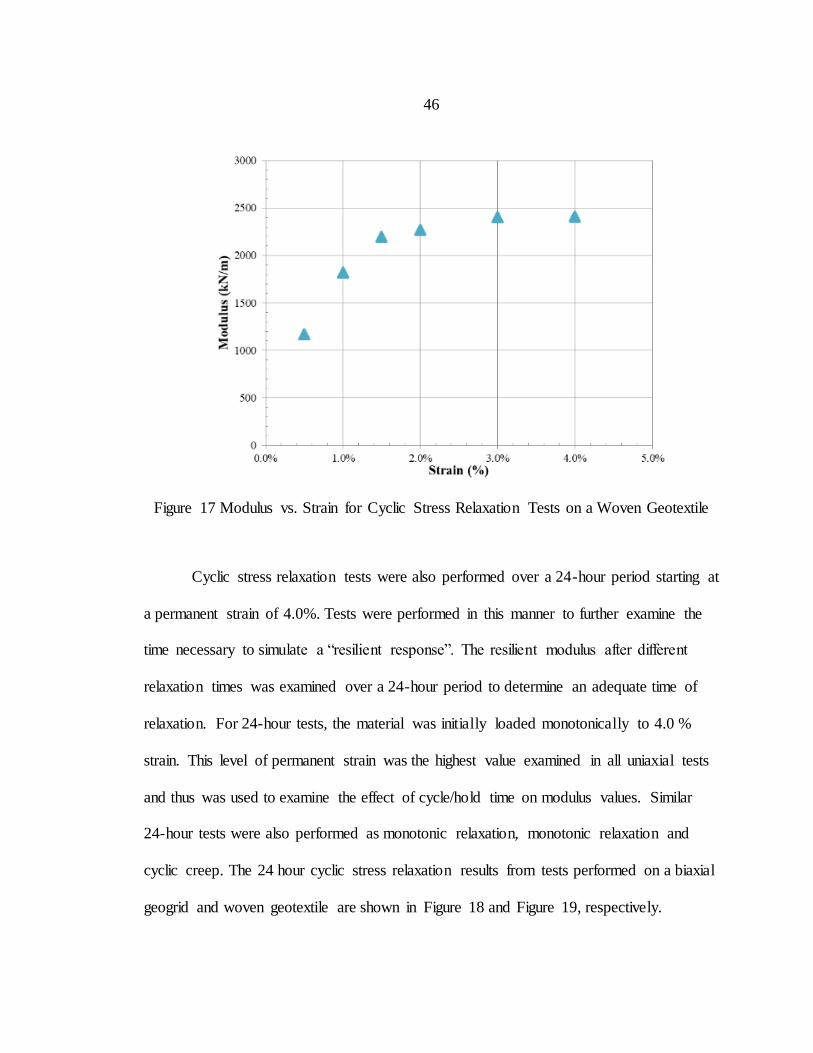
46
Figure 17 Modulus vs. Strain for Cyclic Stress Relaxation Tests on a Woven Geotextile
Cyclic stress relaxation tests were also performed over a 24-hour period starting at
a permanent strain of 4.0%. Tests were performed in this manner to further examine the
time necessary to simulate a “resilient response”. The resilient modulus after different
relaxation times was examined over a 24-hour period to determine an adequate time of
relaxation. For 24-hour tests, the material was initially loaded monotonically to 4.0 %
strain. This level of permanent strain was the highest value examined in all uniaxial tests
and thus was used to examine the effect of cycle/hold time on modulus values. Similar
24-hour tests were also performed as monotonic relaxation, monotonic relaxation and
cyclic creep. The 24 hour cyclic stress relaxation results from tests performed on a biaxial
geogrid and woven geotextile are shown in Figure 18 and Figure 19, respectively.
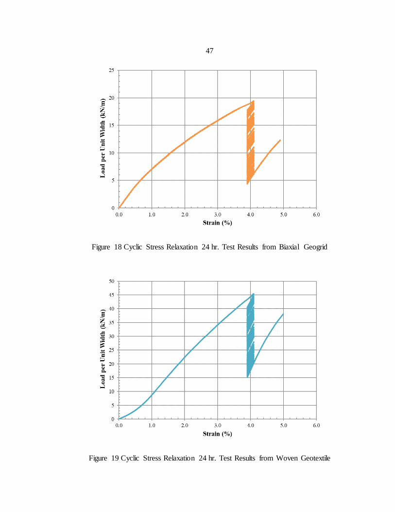
47
Figure 18 Cyclic Stress Relaxation 24 hr. Test Results from Biaxial Geogrid
Figure 19 Cyclic Stress Relaxation 24 hr. Test Results from Woven Geotextile
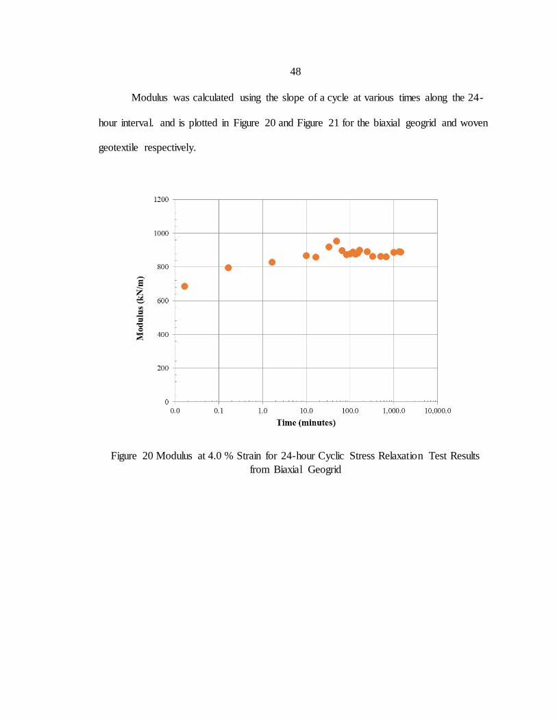
48
Modulus was calculated using the slope of a cycle at various times along the 24-
hour interval. and is plotted in Figure 20 and Figure 21 for the biaxial geogrid and woven
geotextile respectively.
Figure 20 Modulus at 4.0 % Strain for 24-hour Cyclic Stress Relaxation Test Results
from Biaxial Geogrid
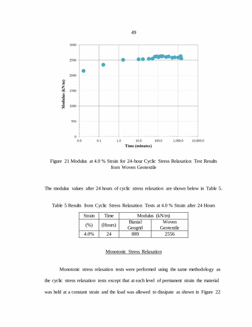
49
Figure 21 Modulus at 4.0 % Strain for 24-hour Cyclic Stress Relaxation Test Results
from Woven Geotextile
The modulus values after 24 hours of cyclic stress relaxation are shown below in Table 5.
Table 5 Results from Cyclic Stress Relaxation Tests at 4.0 % Strain after 24 Hours
Strain Time Modulus (kN/m)
(%) (Hours) Biaxial
Geogrid
Woven
Geotextile
4.0% 24 889 2556
Monotonic Stress Relaxation
Monotonic stress relaxation tests were performed using the same methodology as
the cyclic stress relaxation tests except that at each level of permanent strain the material
was held at a constant strain and the load was allowed to dissipate as shown in Figure 22
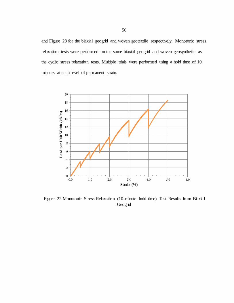
50
and Figure 23 for the biaxial geogrid and woven geotextile respectively. Monotonic stress
relaxation tests were performed on the same biaxial geogrid and woven geosynthetic as
the cyclic stress relaxation tests. Multiple trials were performed using a hold time of 10
minutes at each level of permanent strain.
Figure 22 Monotonic Stress Relaxation (10-minute hold time) Test Results from Biaxial
Geogrid
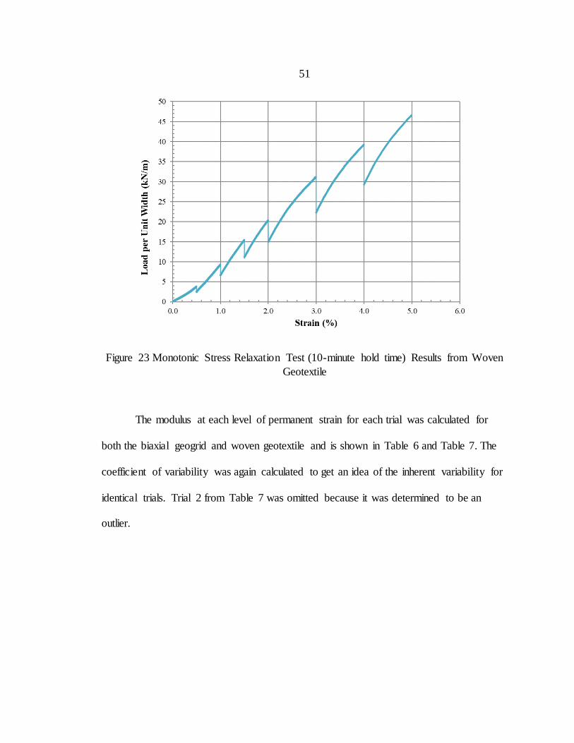
51
Figure 23 Monotonic Stress Relaxation Test (10-minute hold time) Results from Woven
Geotextile
The modulus at each level of permanent strain for each trial was calculated for
both the biaxial geogrid and woven geotextile and is shown in Table 6 and Table 7. The
coefficient of variability was again calculated to get an idea of the inherent variability for
identical trials. Trial 2 from Table 7 was omitted because it was determined to be an
outlier.
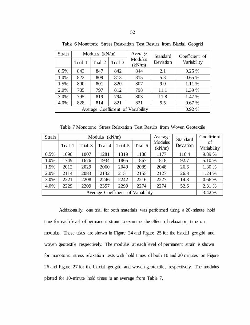
52
Table 6 Monotonic Stress Relaxation Test Results from Biaxial Geogrid
Strain Modulus (kN/m) Average
Modulus (kN/m)
Standard
Deviation
Coefficient of
Variability Trial 1 Trial 2 Trial 3
0.5% 843 847 842 844 2.1 0.25 %
1.0% 822 809 813 815 5.3 0.65 %
1.5% 800 801 820 807 9.0 1.11 %
2.0% 785 797 812 798 11.1 1.39 %
3.0% 795 819 794 803 11.8 1.47 %
4.0% 828 814 821 821 5.5 0.67 %
Average Coefficient of Variability 0.92 %
Table 7 Monotonic Stress Relaxation Test Results from Woven Geotextile
Strain Modulus (kN/m) Average Modulus
(kN/m)
Standard
Deviation
Coefficient of
Variability Trial 1 Trial 3 Trial 4 Trial 5 Trial 6
0.5% 1090 1007 1281 1319 1188 1177 116.4 9.89 %
1.0% 1749 1676 1934 1865 1867 1818 92.7 5.10 %
1.5% 2012 2029 2060 2049 2089 2048 26.6 1.30 %
2.0% 2114 2083 2132 2151 2155 2127 26.3 1.24 %
3.0% 2221 2208 2246 2242 2216 2227 14.8 0.66 %
4.0% 2229 2209 2357 2299 2274 2274 52.6 2.31 %
Average Coefficient of Variability 3.42 %
Additionally, one trial for both materials was performed using a 20-minute hold
time for each level of permanent strain to examine the effect of relaxation time on
modulus. These trials are shown in Figure 24 and Figure 25 for the biaxial geogrid and
woven geotextile respectively. The modulus at each level of permanent strain is shown
for monotonic stress relaxation tests with hold times of both 10 and 20 minutes on Figure
26 and Figure 27 for the biaxial geogrid and woven geotextile, respectively. The modulus
plotted for 10-minute hold times is an average from Table 7.
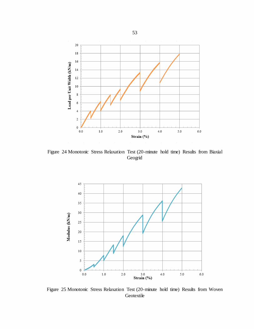
53
Figure 24 Monotonic Stress Relaxation Test (20-minute hold time) Results from Biaxial
Geogrid
Figure 25 Monotonic Stress Relaxation Test (20-minute hold time) Results from Woven
Geotextile
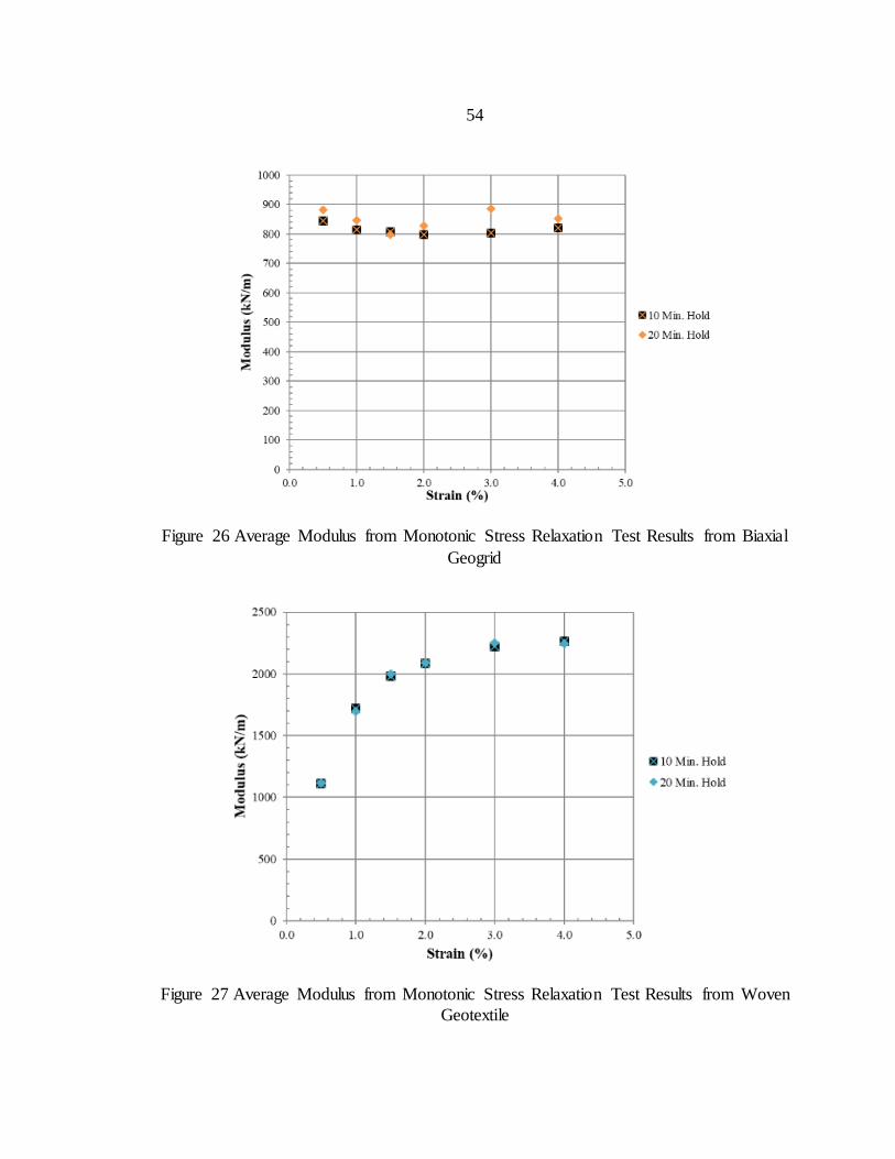
54
Figure 26 Average Modulus from Monotonic Stress Relaxation Test Results from Biaxial
Geogrid
Figure 27 Average Modulus from Monotonic Stress Relaxation Test Results from Woven
Geotextile
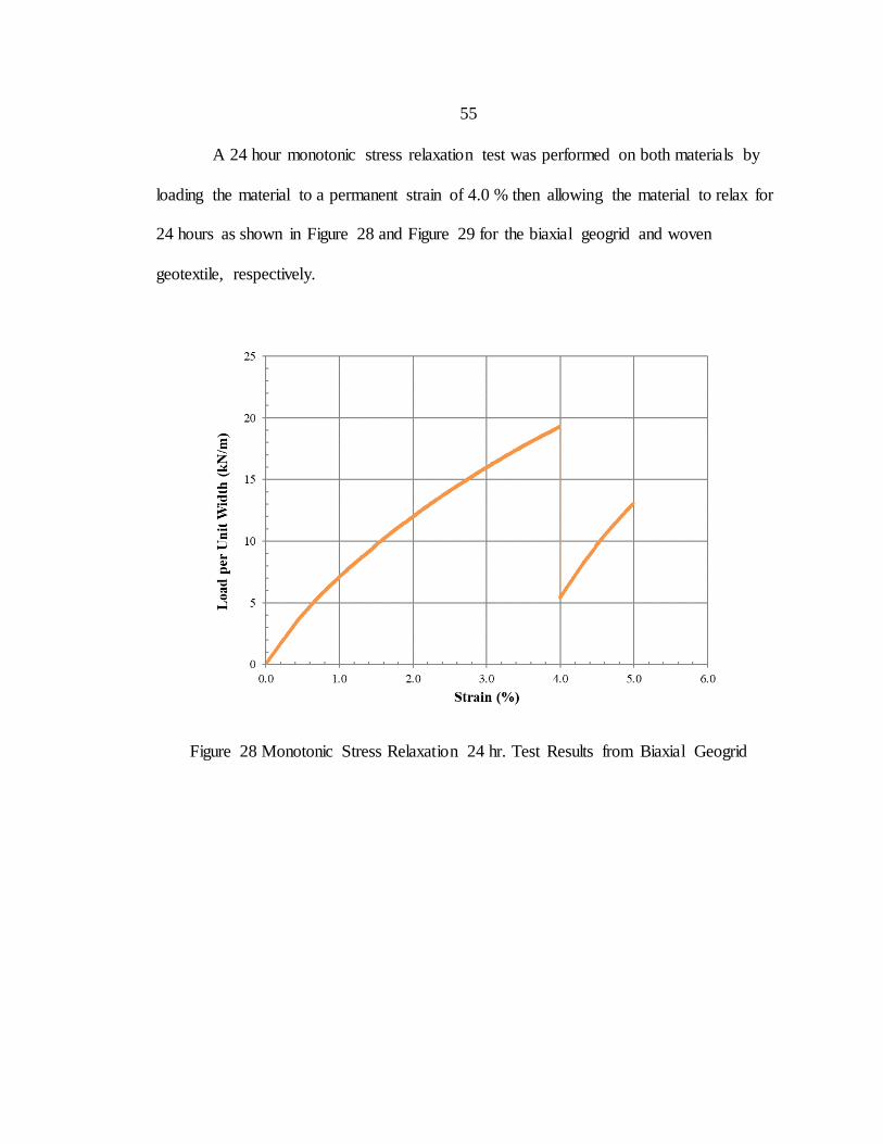
55
A 24 hour monotonic stress relaxation test was performed on both materials by
loading the material to a permanent strain of 4.0 % then allowing the material to relax for
24 hours as shown in Figure 28 and Figure 29 for the biaxial geogrid and woven
geotextile, respectively.
Figure 28 Monotonic Stress Relaxation 24 hr. Test Results from Biaxial Geogrid
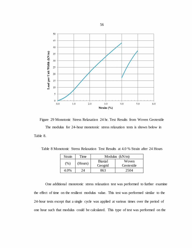
56
Figure 29 Monotonic Stress Relaxation 24 hr. Test Results from Woven Geotextile
The modulus for 24-hour monotonic stress relaxation tests is shown below in
Table 8.
Table 8 Monotonic Stress Relaxation Test Results at 4.0 % Strain after 24 Hours
Strain Time Modulus (kN/m)
(%) (Hours) Biaxial Geogrid
Woven Geotextile
4.0% 24 863 2504
One additional monotonic stress relaxation test was performed to further examine
the effect of time on the resilient modulus value. This test was performed similar to the
24-hour tests except that a single cycle was applied at various times over the period of
one hour such that modulus could be calculated. This type of test was performed on the
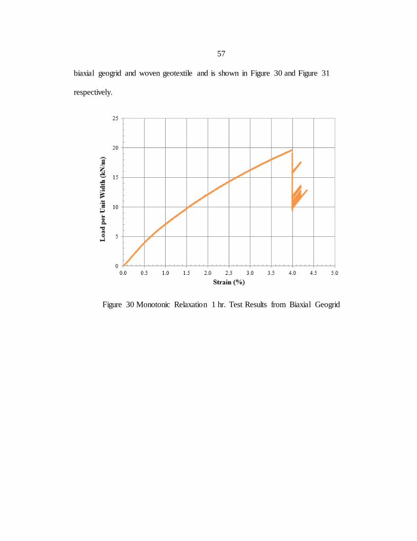
57
biaxial geogrid and woven geotextile and is shown in Figure 30 and Figure 31
respectively.
Figure 30 Monotonic Relaxation 1 hr. Test Results from Biaxial Geogrid
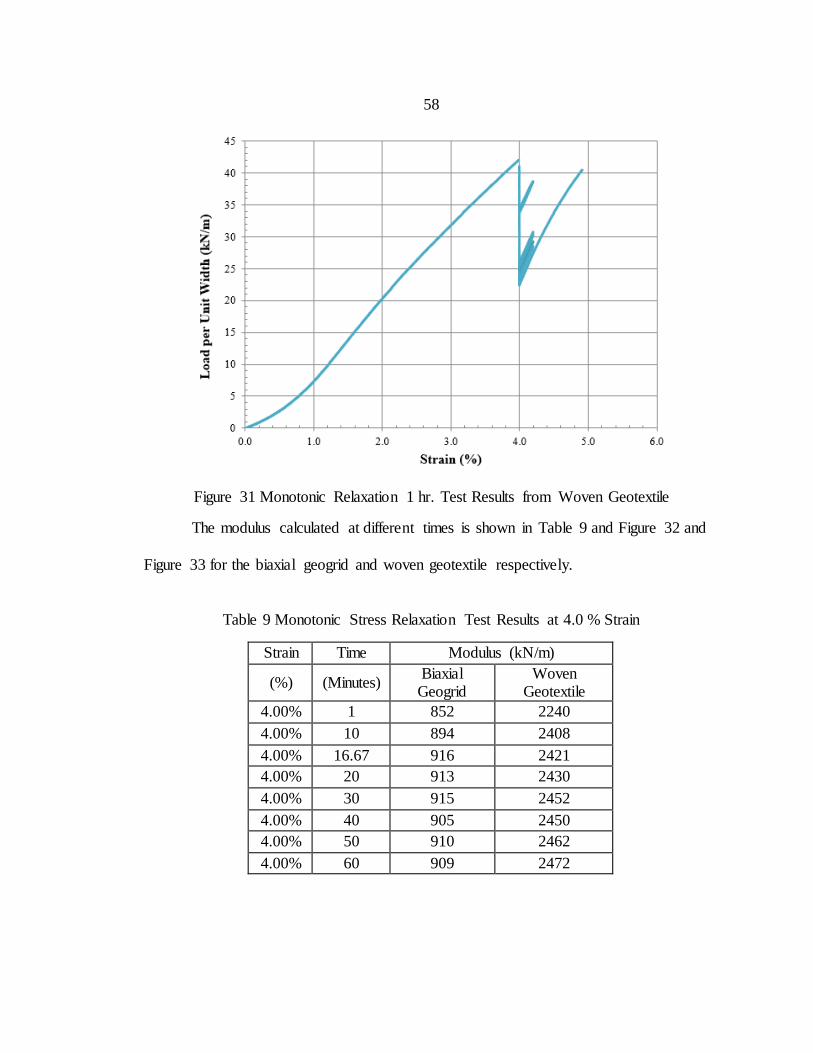
58
Figure 31 Monotonic Relaxation 1 hr. Test Results from Woven Geotextile
The modulus calculated at different times is shown in Table 9 and Figure 32 and
Figure 33 for the biaxial geogrid and woven geotextile respectively.
Table 9 Monotonic Stress Relaxation Test Results at 4.0 % Strain
Strain Time Modulus (kN/m)
(%) (Minutes) Biaxial Geogrid
Woven Geotextile
4.00% 1 852 2240
4.00% 10 894 2408
4.00% 16.67 916 2421
4.00% 20 913 2430
4.00% 30 915 2452
4.00% 40 905 2450
4.00% 50 910 2462
4.00% 60 909 2472
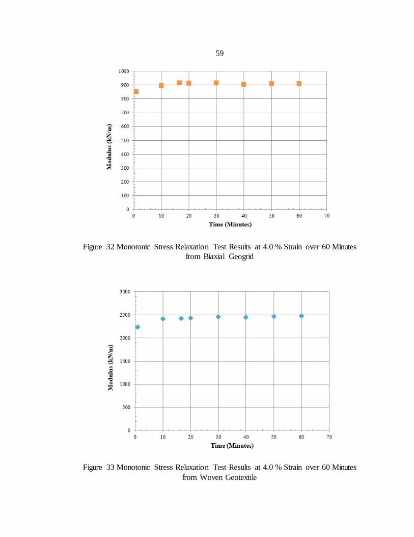
59
Figure 32 Monotonic Stress Relaxation Test Results at 4.0 % Strain over 60 Minutes
from Biaxial Geogrid
Figure 33 Monotonic Stress Relaxation Test Results at 4.0 % Strain over 60 Minutes
from Woven Geotextile
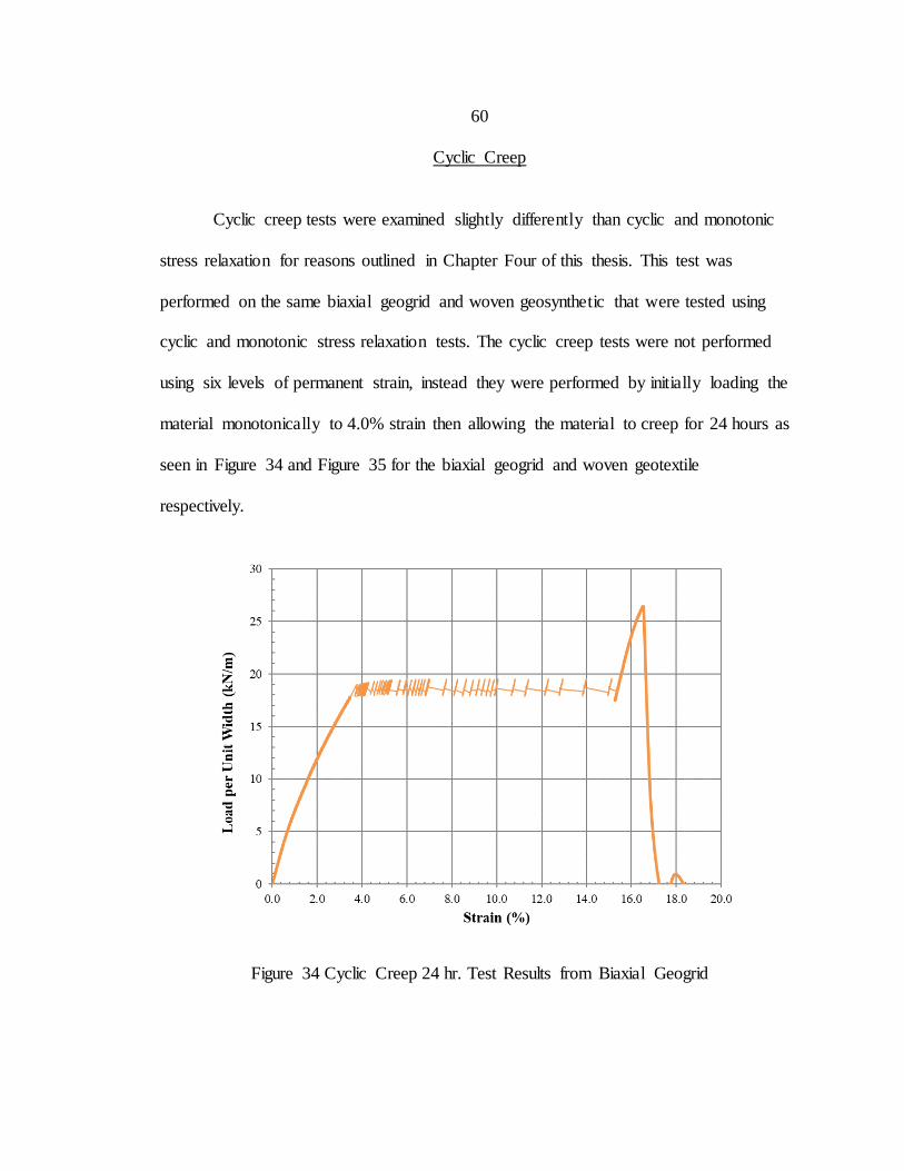
60
Cyclic Creep
Cyclic creep tests were examined slightly differently than cyclic and monotonic
stress relaxation for reasons outlined in Chapter Four of this thesis. This test was
performed on the same biaxial geogrid and woven geosynthetic that were tested using
cyclic and monotonic stress relaxation tests. The cyclic creep tests were not performed
using six levels of permanent strain, instead they were performed by initially loading the
material monotonically to 4.0% strain then allowing the material to creep for 24 hours as
seen in Figure 34 and Figure 35 for the biaxial geogrid and woven geotextile
respectively.
Figure 34 Cyclic Creep 24 hr. Test Results from Biaxial Geogrid
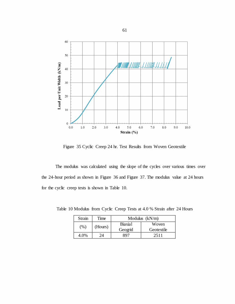
61
Figure 35 Cyclic Creep 24 hr. Test Results from Woven Geotextile
The modulus was calculated using the slope of the cycles over various times over
the 24-hour period as shown in Figure 36 and Figure 37. The modulus value at 24 hours
for the cyclic creep tests is shown in Table 10.
Table 10 Modulus from Cyclic Creep Tests at 4.0 % Strain after 24 Hours
Strain Time Modulus (kN/m)
(%) (Hours) Biaxial
Geogrid
Woven
Geotextile
4.0% 24 897 2511
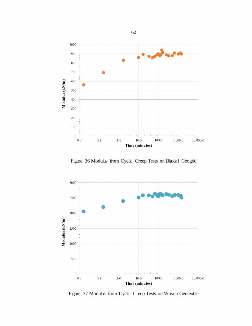
62
Figure 36 Modulus from Cyclic Creep Tests on Biaxial Geogrid
Figure 37 Modulus from Cyclic Creep Tests on Woven Geotextile
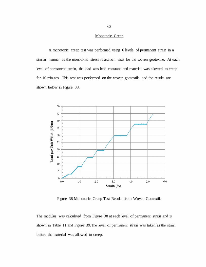
63
Monotonic Creep
A monotonic creep test was performed using 6 levels of permanent strain in a
similar manner as the monotonic stress relaxation tests for the woven geotextile. At each
level of permanent strain, the load was held constant and material was allowed to creep
for 10 minutes. This test was performed on the woven geotextile and the results are
shown below in Figure 38.
Figure 38 Monotonic Creep Test Results from Woven Geotextile
The modulus was calculated from Figure 38 at each level of permanent strain and is
shown in Table 11 and Figure 39.The level of permanent strain was taken as the strain
before the material was allowed to creep.
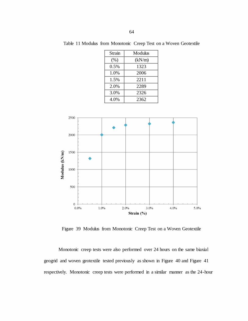
64
Table 11 Modulus from Monotonic Creep Test on a Woven Geotextile
Strain Modulus
(%) (kN/m)
0.5% 1323
1.0% 2006
1.5% 2211
2.0% 2289
3.0% 2326
4.0% 2362
Figure 39 Modulus from Monotonic Creep Test on a Woven Geotextile
Monotonic creep tests were also performed over 24 hours on the same biaxial
geogrid and woven geotextile tested previously as shown in Figure 40 and Figure 41
respectively. Monotonic creep tests were performed in a similar manner as the 24-hour
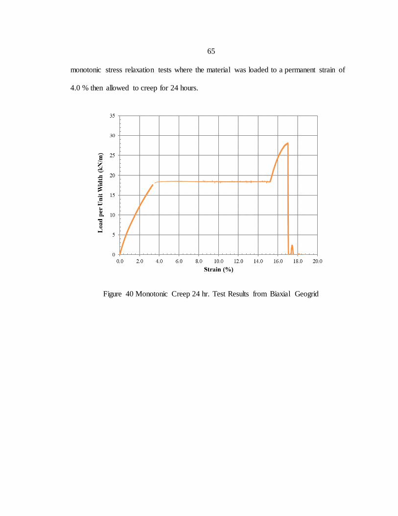
65
monotonic stress relaxation tests where the material was loaded to a permanent strain of
4.0 % then allowed to creep for 24 hours.
Figure 40 Monotonic Creep 24 hr. Test Results from Biaxial Geogrid
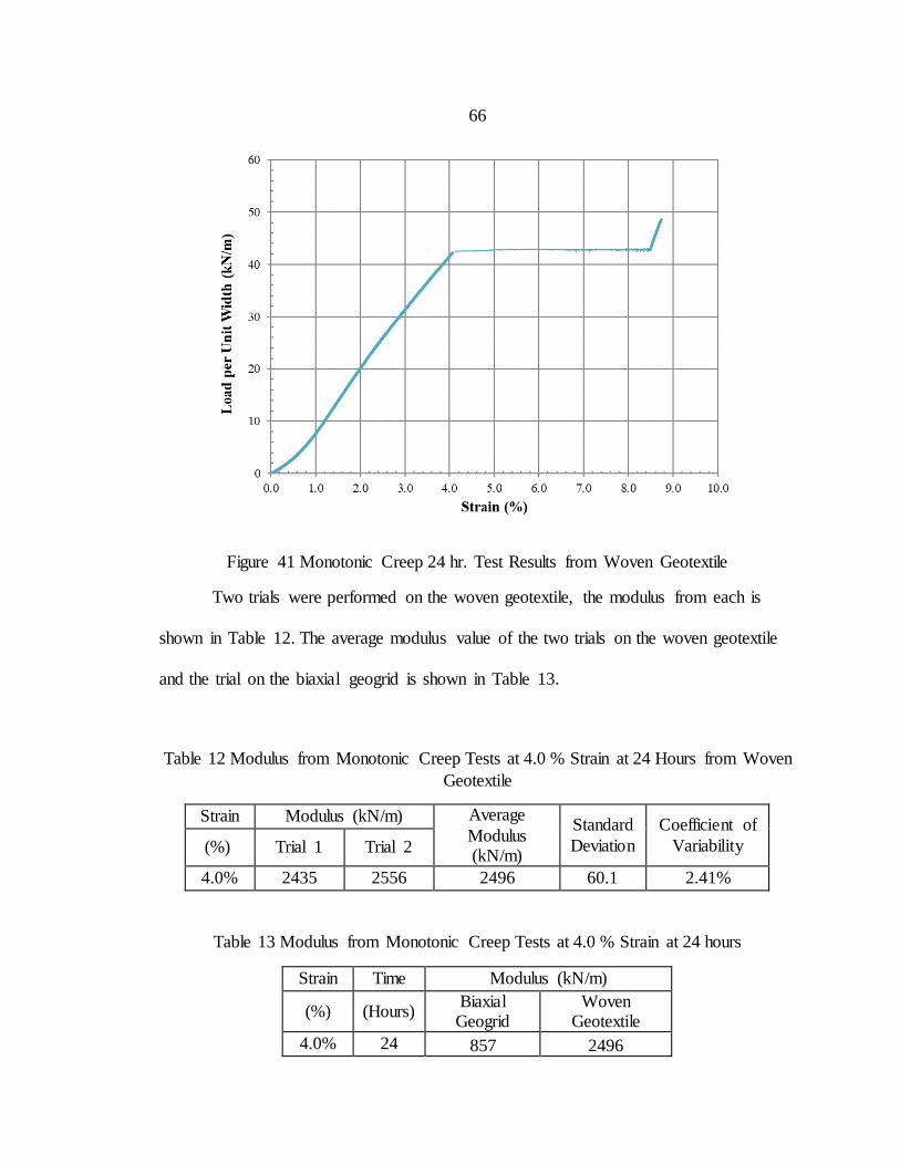
66
Figure 41 Monotonic Creep 24 hr. Test Results from Woven Geotextile
Two trials were performed on the woven geotextile, the modulus from each is
shown in Table 12. The average modulus value of the two trials on the woven geotextile
and the trial on the biaxial geogrid is shown in Table 13.
Table 12 Modulus from Monotonic Creep Tests at 4.0 % Strain at 24 Hours from Woven
Geotextile
Strain Modulus (kN/m) Average
Modulus (kN/m)
Standard
Deviation
Coefficient of
Variability (%) Trial 1 Trial 2
4.0% 2435 2556 2496 60.1 2.41%
Table 13 Modulus from Monotonic Creep Tests at 4.0 % Strain at 24 hours
Strain Time Modulus (kN/m)
(%) (Hours) Biaxial Geogrid
Woven Geotextile
4.0% 24 857 2496
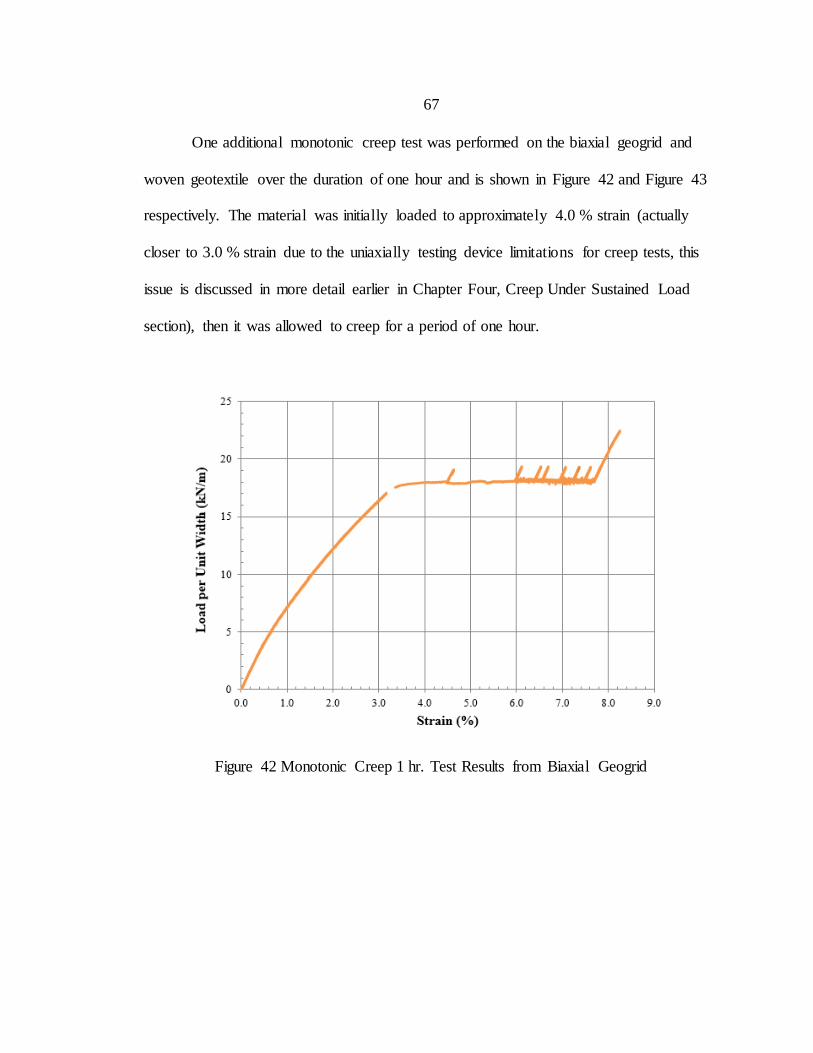
67
One additional monotonic creep test was performed on the biaxial geogrid and
woven geotextile over the duration of one hour and is shown in Figure 42 and Figure 43
respectively. The material was initially loaded to approximately 4.0 % strain (actually
closer to 3.0 % strain due to the uniaxially testing device limitations for creep tests, this
issue is discussed in more detail earlier in Chapter Four, Creep Under Sustained Load
section), then it was allowed to creep for a period of one hour.
Figure 42 Monotonic Creep 1 hr. Test Results from Biaxial Geogrid
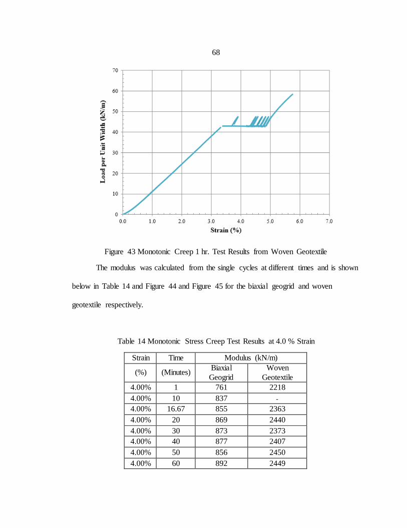
68
Figure 43 Monotonic Creep 1 hr. Test Results from Woven Geotextile
The modulus was calculated from the single cycles at different times and is shown
below in Table 14 and Figure 44 and Figure 45 for the biaxial geogrid and woven
geotextile respectively.
Table 14 Monotonic Stress Creep Test Results at 4.0 % Strain
Strain Time Modulus (kN/m)
(%) (Minutes) Biaxial
Geogrid
Woven
Geotextile
4.00% 1 761 2218
4.00% 10 837 -
4.00% 16.67 855 2363
4.00% 20 869 2440
4.00% 30 873 2373
4.00% 40 877 2407
4.00% 50 856 2450
4.00% 60 892 2449
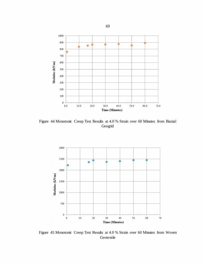
69
Figure 44 Monotonic Creep Test Results at 4.0 % Strain over 60 Minutes from Biaxial
Geogrid
Figure 45 Monotonic Creep Test Results at 4.0 % Strain over 60 Minutes from Woven
Geotextile
70
Analysis of Uniaxial Testing
The goal of the uniaxial testing program was to examine the resilient response of
geosynthetics subjected to different types of loading over different durations of time to
help develop a biaxial testing procedure using the biaxial device available. To do this, it
was necessary to examine the resilient response from cyclic and monotonic stress
relaxation and creep tests. It was also necessary to determine an adequate time to allow
the material to relax/creep at each level of permanent strain such that the resilient
response measured adequately described the resilient response expected in field loadings.
The modulus from tests performed at six levels of permanent strain are compared on
Figure 46 and Figure 47 for the biaxial geogrid and woven geotextile, respectively. The
tests that were loaded initially to 4.0 % permanent strain were allowed to relax or creep
for 24 hours are also shown on Figure 46 and Figure 47.
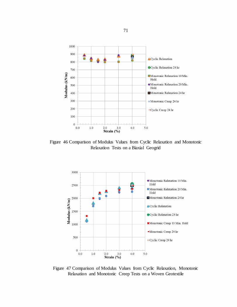
71
Figure 46 Comparison of Modulus Values from Cyclic Relaxation and Monotonic
Relaxation Tests on a Biaxial Geogrid
Figure 47 Comparison of Modulus Values from Cyclic Relaxation, Monotonic
Relaxation and Monotonic Creep Tests on a Woven Geotextile
72
Cyclic and monotonic stress relaxation tests were performed extensively on both
the biaxial geogrid and woven geotextile. For each of these types of tests, multiple trials
were performed on each material such that a modulus was calculated at five or six levels
of permanent strain. The modulus values could then be examined statistically to see the
coefficient of variability that represents the variation in modulus values from the same
type of test. This baseline variability should not increase when the modulus from
different types of tests are compared if these modes of loading in fact are equivalent.
Examining Table 3, Table 4, Table 6, Table 7 and Table 12 the variability of modulus
values for cyclic stress relaxation (Table 3 and Table 4), monotonic stress relaxation
(Table 6 and Table 7) and monotonic creep (Table 12) is observed. The coefficient of
variability for modulus values from identical tests ranged from 0.25 % to 9.89 %.
To first examine the difference between cycling a material over small strains
(±0.1 %) versus holding the material under a sustained strain (monotonic relaxation), the
average modulus value for each level of permanent strain from cyclic stress relaxation
(1000 cycles) and monotonic stress relaxation (10 minute holds) were compared as
shown below in Table 15 and Table 16 for the biaxial geogrid and woven geotextile
respectively.
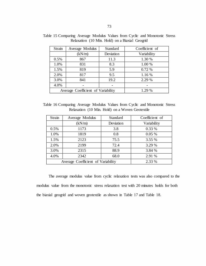
73
Table 15 Comparing Average Modulus Values from Cyclic and Monotonic Stress
Relaxation (10 Min. Hold) on a Biaxial Geogrid
Strain Average Modulus Standard Coefficient of
(kN/m) Deviation Variability
0.5% 867 11.3 1.30 %
1.0% 831 8.3 1.00 %
1.5% 819 5.9 0.72 %
2.0% 817 9.5 1.16 %
3.0% 841 19.2 2.29 %
4.0% - - -
Average Coefficient of Variability 1.29 %
Table 16 Comparing Average Modulus Values from Cyclic and Monotonic Stress
Relaxation (10 Min. Hold) on a Woven Geotextile
Strain Average Modulus Standard Coefficient of
(kN/m) Deviation Variability
0.5% 1173 3.8 0.33 %
1.0% 1819 0.8 0.05 %
1.5% 2123 75.5 3.55 %
2.0% 2199 72.4 3.29 %
3.0% 2315 88.9 3.84 %
4.0% 2342 68.0 2.91 %
Average Coefficient of Variability 2.33 %
The average modulus value from cyclic relaxation tests was also compared to the
modulus value from the monotonic stress relaxation test with 20 minutes holds for both
the biaxial geogrid and woven geotextile as shown in Table 17 and Table 18.
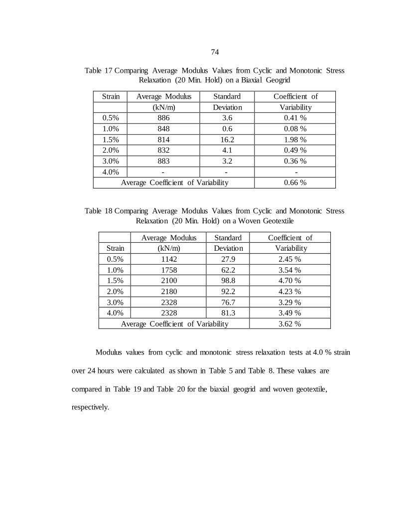
74
Table 17 Comparing Average Modulus Values from Cyclic and Monotonic Stress
Relaxation (20 Min. Hold) on a Biaxial Geogrid
Strain Average Modulus Standard Coefficient of
(kN/m) Deviation Variability
0.5% 886 3.6 0.41 %
1.0% 848 0.6 0.08 %
1.5% 814 16.2 1.98 %
2.0% 832 4.1 0.49 %
3.0% 883 3.2 0.36 %
4.0% - - -
Average Coefficient of Variability 0.66 %
Table 18 Comparing Average Modulus Values from Cyclic and Monotonic Stress
Relaxation (20 Min. Hold) on a Woven Geotextile
Average Modulus Standard Coefficient of
Strain (kN/m) Deviation Variability
0.5% 1142 27.9 2.45 %
1.0% 1758 62.2 3.54 %
1.5% 2100 98.8 4.70 %
2.0% 2180 92.2 4.23 %
3.0% 2328 76.7 3.29 %
4.0% 2328 81.3 3.49 %
Average Coefficient of Variability 3.62 %
Modulus values from cyclic and monotonic stress relaxation tests at 4.0 % strain
over 24 hours were calculated as shown in Table 5 and Table 8. These values are
compared in Table 19 and Table 20 for the biaxial geogrid and woven geotextile,
respectively.

75
Table 19 Comparing Modulus Values from 24 Hr. Cyclic and Monotonic Stress
Relaxation on a Biaxial Geogrid
Strain Average Modulus Standard Coefficient of
(kN/m) Deviation Variability
4.00% 876 12.9 1.47%
Table 20 Comparing Modulus Values from 24 Hr. Cyclic and Monotonic Stress
Relaxation on a Woven Geotextile
Strain Average Modulus Standard Coefficient of
(kN/m) Deviation Variability
4.00% 2530 26.1 1.03%
Using the same data compared in Table 19 and Table 20 with the addition of the
data from Table 10 and Table 13, the modulus at 4.0 % strain can be compared from
cyclic and monotonic stress relaxation and creep. This is shown below in Table 21 and
Table 22 for the biaxial geogrid and woven geotextile respectively.
Table 21 Comparing Modulus Values from 24 Hr. Cyclic and Monotonic Stress
Relaxation and Creep on a Biaxial Geogrid
Strain Average Modulus Standard Coefficient of
(kN/m) Deviation Variability
4.00% 876 16.8 1.92%
Table 22 Comparing Modulus Values from 24 Hr. Cyclic and Monotonic Stress
Relaxation and Creep on a Woven Geotextile
Strain Average Modulus Standard Coefficient of
(kN/m) Deviation Variability
4.00% 2517 23.5 0.93%
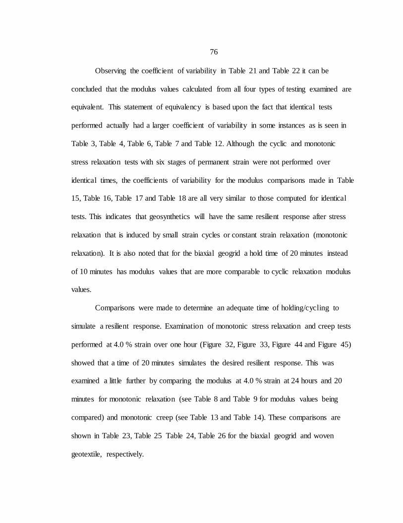
76
Observing the coefficient of variability in Table 21 and Table 22 it can be
concluded that the modulus values calculated from all four types of testing examined are
equivalent. This statement of equivalency is based upon the fact that identical tests
performed actually had a larger coefficient of variability in some instances as is seen in
Table 3, Table 4, Table 6, Table 7 and Table 12. Although the cyclic and monotonic
stress relaxation tests with six stages of permanent strain were not performed over
identical times, the coefficients of variability for the modulus comparisons made in Table
15, Table 16, Table 17 and Table 18 are all very similar to those computed for identical
tests. This indicates that geosynthetics will have the same resilient response after stress
relaxation that is induced by small strain cycles or constant strain relaxation (monotonic
relaxation). It is also noted that for the biaxial geogrid a hold time of 20 minutes instead
of 10 minutes has modulus values that are more comparable to cyclic relaxation modulus
values.
Comparisons were made to determine an adequate time of holding/cycling to
simulate a resilient response. Examination of monotonic stress relaxation and creep tests
performed at 4.0 % strain over one hour (Figure 32, Figure 33, Figure 44 and Figure 45)
showed that a time of 20 minutes simulates the desired resilient response. This was
examined a little further by comparing the modulus at 4.0 % strain at 24 hours and 20
minutes for monotonic relaxation (see Table 8 and Table 9 for modulus values being
compared) and monotonic creep (see Table 13 and Table 14). These comparisons are
shown in Table 23, Table 25 Table 24, Table 26 for the biaxial geogrid and woven
geotextile, respectively.
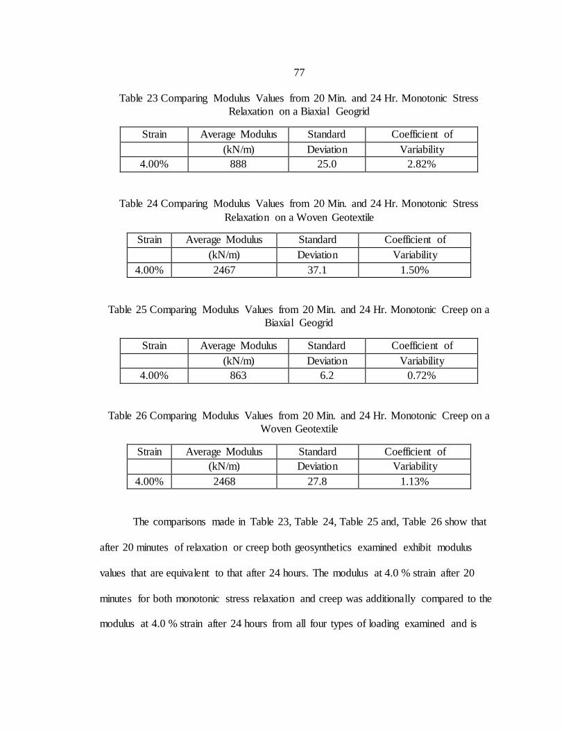
77
Table 23 Comparing Modulus Values from 20 Min. and 24 Hr. Monotonic Stress
Relaxation on a Biaxial Geogrid
Strain Average Modulus Standard Coefficient of
(kN/m) Deviation Variability
4.00% 888 25.0 2.82%
Table 24 Comparing Modulus Values from 20 Min. and 24 Hr. Monotonic Stress
Relaxation on a Woven Geotextile
Strain Average Modulus Standard Coefficient of
(kN/m) Deviation Variability
4.00% 2467 37.1 1.50%
Table 25 Comparing Modulus Values from 20 Min. and 24 Hr. Monotonic Creep on a
Biaxial Geogrid
Strain Average Modulus Standard Coefficient of
(kN/m) Deviation Variability
4.00% 863 6.2 0.72%
Table 26 Comparing Modulus Values from 20 Min. and 24 Hr. Monotonic Creep on a
Woven Geotextile
Strain Average Modulus Standard Coefficient of
(kN/m) Deviation Variability
4.00% 2468 27.8 1.13%
The comparisons made in Table 23, Table 24, Table 25 and, Table 26 show that
after 20 minutes of relaxation or creep both geosynthetics examined exhibit modulus
values that are equivalent to that after 24 hours. The modulus at 4.0 % strain after 20
minutes for both monotonic stress relaxation and creep was additionally compared to the
modulus at 4.0 % strain after 24 hours from all four types of loading examined and is
78
shown in Table 27 and Table 28 for the biaxial geogrid and woven geotextile
respectively.
Table 27 Comparing Modulus Values from 20 Min. Monotonic Creep and Relaxation, 24
Hr. Monotonic and Cyclic Stress Relaxation and Creep on a Biaxial Geogrid
Strain Average Modulus Standard Coefficient of
(kN/m) Deviation Variability
4.00% 881 20.0 2.27%
Table 28 Comparing Modulus Values from 20 Min. Monotonic Creep and Relaxation, 24
Hr. Monotonic and Cyclic Stress Relaxation and Creep on a Biaxial Geogrid
Strain Average Modulus Standard Coefficient of
(kN/m) Deviation Variability
4.00% 2490 43.1 1.73%
The comparisons made in Table 27 and Table 28 show that after 20 minutes of
relaxation or creep the resilient modulus calculated is equivalent to that of a resilient
modulus after 24 hours. Table 27 and Table 28 also again demonstrate that all four types
of loading are equivalent for calculation of a resilient modulus. Equivalency is based
upon the fact that the coefficients of variability observed when comparing dissimilar
types of tests is within the range of coefficients of variability that were calculated for
identical tests with multiple trials.
Conclusions from Uniaxial Testing
It has been shown in this chapter of this thesis that the four forms of loading
examined (Cyclic Stress Relaxation, Cyclic Creep, Monotonic Stress Relaxation and
Monotonic Creep) result in equivalent resilient responses of two different geosynthetic
79
materials. It has also been shown that a time of 20 minutes results in an equivalent
resilient response as a time of 24 hours for the two different geosynthetics examined. The
biaxial geogrid examined for uniaxial testing was deemed representative of the other
biaxial geogrids that were examined in the biaxial testing program. The woven geotextile
examined in the uniaxial testing program was also deemed representative of the woven
geotextiles that were examined using biaxial tension tests. Thus, a biaxial testing
procedure was created using the knowledge gained from the uniaxial testing program
described in this chapter. The fact that the biaxial device cannot produce purely stress
relaxation was not important for simulating a resilient response of geosynthetics. The
combination of mostly stress relaxation and some stress creep that occurs in biaxial
samples from monotonic tests at multiple permanent strain limits is representative of a
resilient response. A time of 20 minutes at each level of permanent strain was used for
biaxial tests because this was shown to be an adequate time to generate a resilient
response.
80
CHAPTER SIX
BIAXIAL TESTING
Biaxial Testing Methods
The uniaxial testing program was conducted to develop a biaxial testing
procedure that could be used to simulate the resilient response of geosynthetics. The
resilient response for biaxial tension tests is characterized by a more complex model than
uniaxial testing as outlined in the Theory section of this thesis. This more complex model
provides a better representation of field loading conditions of geosynthetics than uniaxial
tests. The biaxial testing procedure developed for this research was based upon ASTM
D7556 with the findings from the uniaxial testing program implemented. This meant that
tests were performed at six permanent strain limits of 0.5, 1.0, 1.5, 2.0, 3.0 and 4.0 %
strain with a hold time of 20 minutes at each level of permanent strain. The material
experienced mostly stress relaxation with some creep during this 20-minute time period.
Three modes of biaxial tension tests were performed to calculate elastic constants
that represent geosynthetics in different field loading situations. Tests where both
perpendicular directions were pulled in tension by an equal displacement will be referred
to as Mode 1 biaxial tests. Tests where the Machine Direction (MD), referred to as the Y
or 2-Direction in this thesis, was held at a constant displacement while the Cross-
Machine Direction (XMD), referred to as the X or 1-Direction in this thesis, was
displaced will be referred to as Mode 2 biaxial tests. Tests where the XMD was held at a
constant displacement while the MD was displaced will be referred to as Mode 3 biaxial
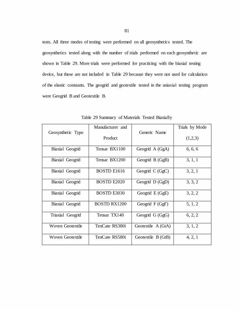
81
tests. All three modes of testing were performed on all geosynthetics tested. The
geosynthetics tested along with the number of trials performed on each geosynthetic are
shown in Table 29. More trials were performed for practicing with the biaxial testing
device, but these are not included in Table 29 because they were not used for calculation
of the elastic constants. The geogrid and geotextile tested in the uniaxial testing program
were Geogrid B and Geotextile B.
Table 29 Summary of Materials Tested Biaxially
Geosynthetic Type Manufacturer and
Product
Generic Name Trials by Mode
(1,2,3)
Biaxial Geogrid Tensar BX1100 Geogrid A (GgA) 6, 6, 6
Biaxial Geogrid Tensar BX1200 Geogrid B (GgB) 3, 1, 1
Biaxial Geogrid BOSTD E1616 Geogrid C (GgC) 3, 2, 1
Biaxial Geogrid BOSTD E2020 Geogrid D (GgD) 3, 3, 2
Biaxial Geogrid BOSTD E3030 Geogrid E (GgE) 3, 2, 2
Biaxial Geogrid BOSTD RX1200 Geogrid F (GgF) 5, 1, 2
Triaxial Geogrid Tensar TX140 Geogrid G (GgG) 6, 2, 2
Woven Geotextile TenCate RS380i Geotextile A (GtA) 3, 1, 2
Woven Geotextile TenCate RS580i Geotextile B (GtB) 4, 2, 1
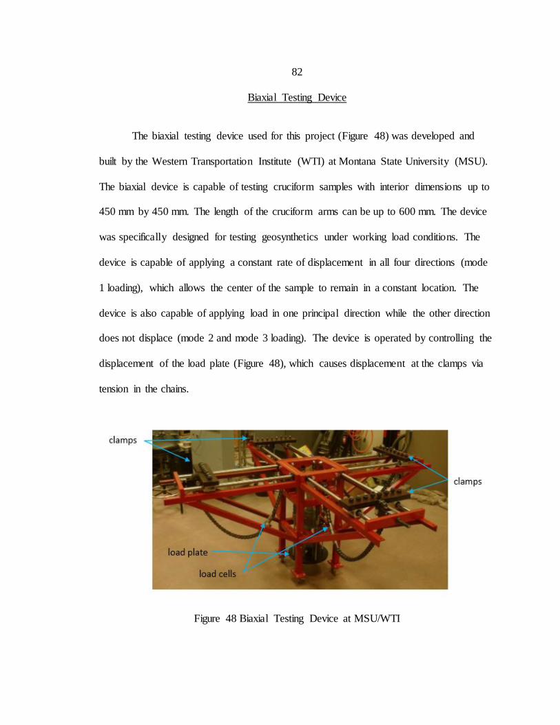
82
Biaxial Testing Device
The biaxial testing device used for this project (Figure 48) was developed and
built by the Western Transportation Institute (WTI) at Montana State University (MSU).
The biaxial device is capable of testing cruciform samples with interior dimensions up to
450 mm by 450 mm. The length of the cruciform arms can be up to 600 mm. The device
was specifically designed for testing geosynthetics under working load conditions. The
device is capable of applying a constant rate of displacement in all four directions (mode
1 loading), which allows the center of the sample to remain in a constant location. The
device is also capable of applying load in one principal direction while the other direction
does not displace (mode 2 and mode 3 loading). The device is operated by controlling the
displacement of the load plate (Figure 48), which causes displacement at the clamps via
tension in the chains.
Figure 48 Biaxial Testing Device at MSU/WTI
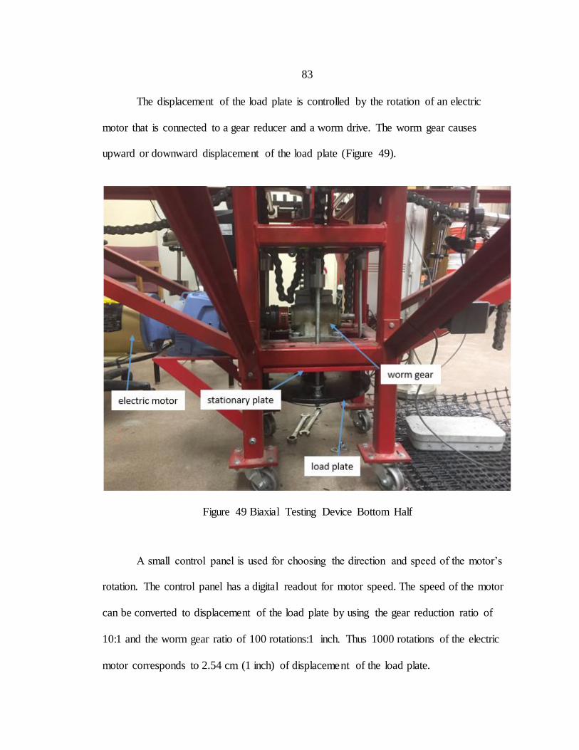
83
The displacement of the load plate is controlled by the rotation of an electric
motor that is connected to a gear reducer and a worm drive. The worm gear causes
upward or downward displacement of the load plate (Figure 49).
Figure 49 Biaxial Testing Device Bottom Half
A small control panel is used for choosing the direction and speed of the motor’s
rotation. The control panel has a digital readout for motor speed. The speed of the motor
can be converted to displacement of the load plate by using the gear reduction ratio of
10:1 and the worm gear ratio of 100 rotations:1 inch. Thus 1000 rotations of the electric
motor corresponds to 2.54 cm (1 inch) of displacement of the load plate.
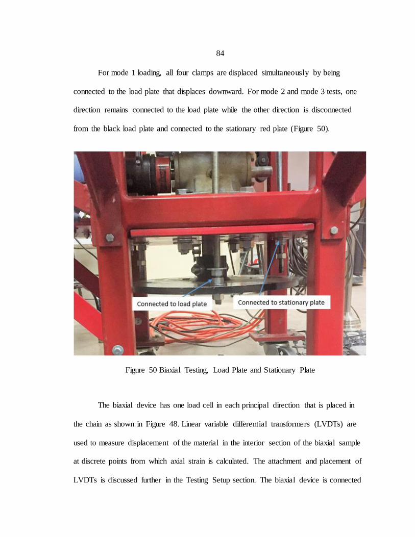
84
For mode 1 loading, all four clamps are displaced simultaneously by being
connected to the load plate that displaces downward. For mode 2 and mode 3 tests, one
direction remains connected to the load plate while the other direction is disconnected
from the black load plate and connected to the stationary red plate (Figure 50).
Figure 50 Biaxial Testing, Load Plate and Stationary Plate
The biaxial device has one load cell in each principal direction that is placed in
the chain as shown in Figure 48. Linear variable differential transformers (LVDTs) are
used to measure displacement of the material in the interior section of the biaxial sample
at discrete points from which axial strain is calculated. The attachment and placement of
LVDTs is discussed further in the Testing Setup section. The biaxial device is connected
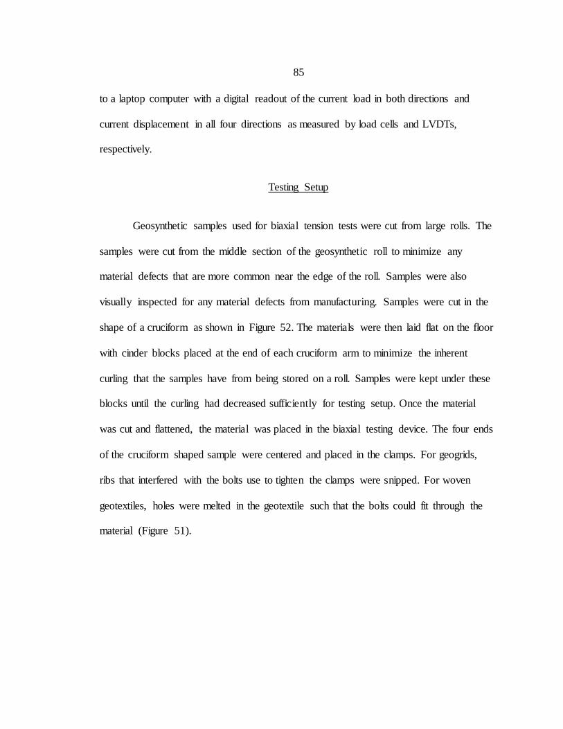
85
to a laptop computer with a digital readout of the current load in both directions and
current displacement in all four directions as measured by load cells and LVDTs,
respectively.
Testing Setup
Geosynthetic samples used for biaxial tension tests were cut from large rolls. The
samples were cut from the middle section of the geosynthetic roll to minimize any
material defects that are more common near the edge of the roll. Samples were also
visually inspected for any material defects from manufacturing. Samples were cut in the
shape of a cruciform as shown in Figure 52. The materials were then laid flat on the floor
with cinder blocks placed at the end of each cruciform arm to minimize the inherent
curling that the samples have from being stored on a roll. Samples were kept under these
blocks until the curling had decreased sufficiently for testing setup. Once the material
was cut and flattened, the material was placed in the biaxial testing device. The four ends
of the cruciform shaped sample were centered and placed in the clamps. For geogrids,
ribs that interfered with the bolts use to tighten the clamps were snipped. For woven
geotextiles, holes were melted in the geotextile such that the bolts could fit through the
material (Figure 51).
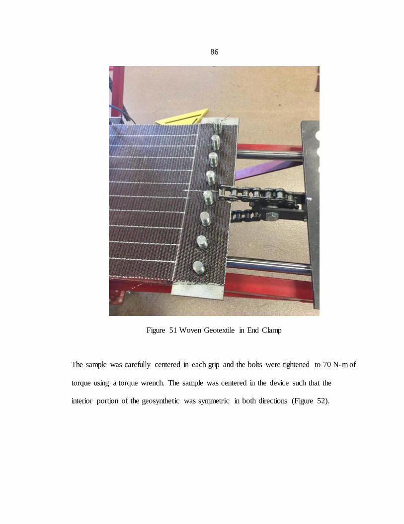
86
Figure 51 Woven Geotextile in End Clamp
The sample was carefully centered in each grip and the bolts were tightened to 70 N-m of
torque using a torque wrench. The sample was centered in the device such that the
interior portion of the geosynthetic was symmetric in both directions (Figure 52).
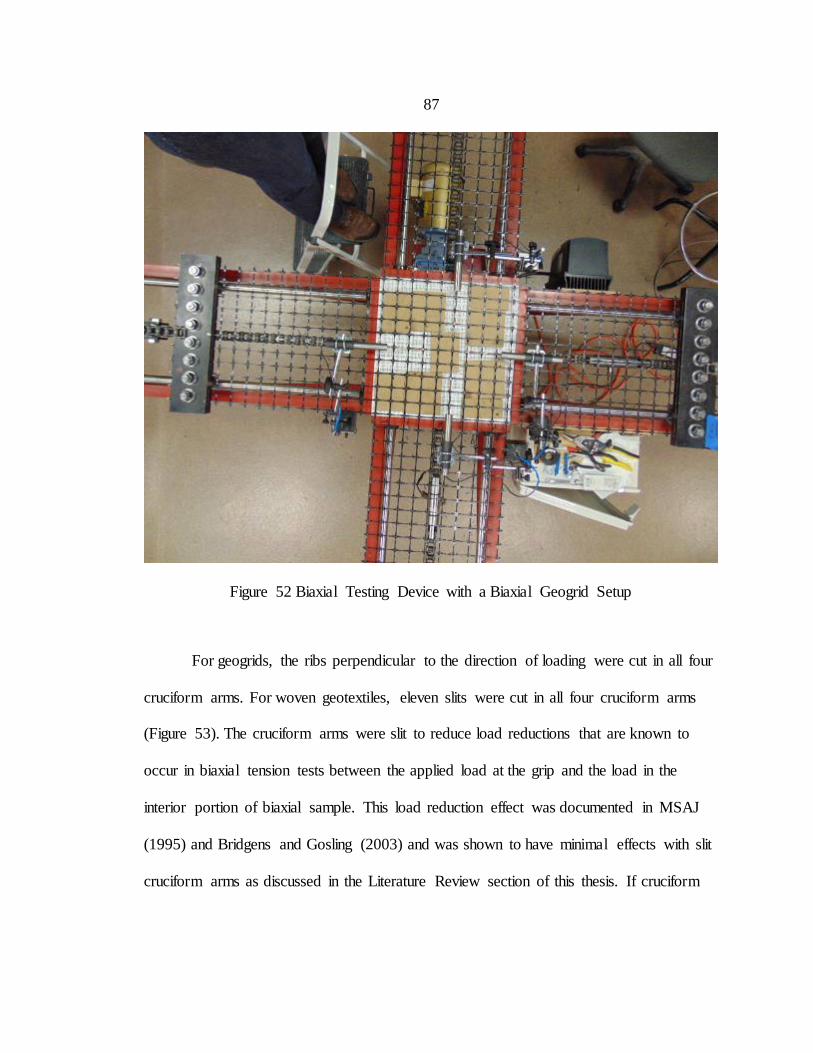
87
Figure 52 Biaxial Testing Device with a Biaxial Geogrid Setup
For geogrids, the ribs perpendicular to the direction of loading were cut in all four
cruciform arms. For woven geotextiles, eleven slits were cut in all four cruciform arms
(Figure 53). The cruciform arms were slit to reduce load reductions that are known to
occur in biaxial tension tests between the applied load at the grip and the load in the
interior portion of biaxial sample. This load reduction effect was documented in MSAJ
(1995) and Bridgens and Gosling (2003) and was shown to have minimal effects with slit
cruciform arms as discussed in the Literature Review section of this thesis. If cruciform
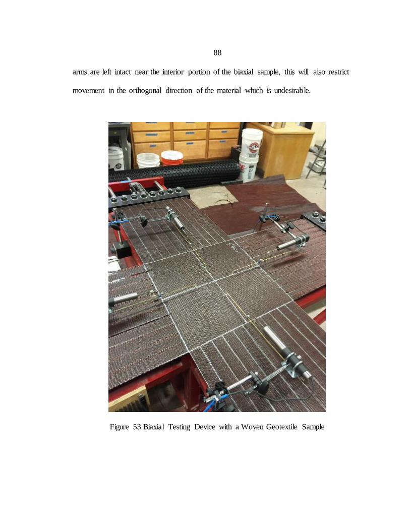
88
arms are left intact near the interior portion of the biaxial sample, this will also restrict
movement in the orthogonal direction of the material which is undesirable.
Figure 53 Biaxial Testing Device with a Woven Geotextile Sample
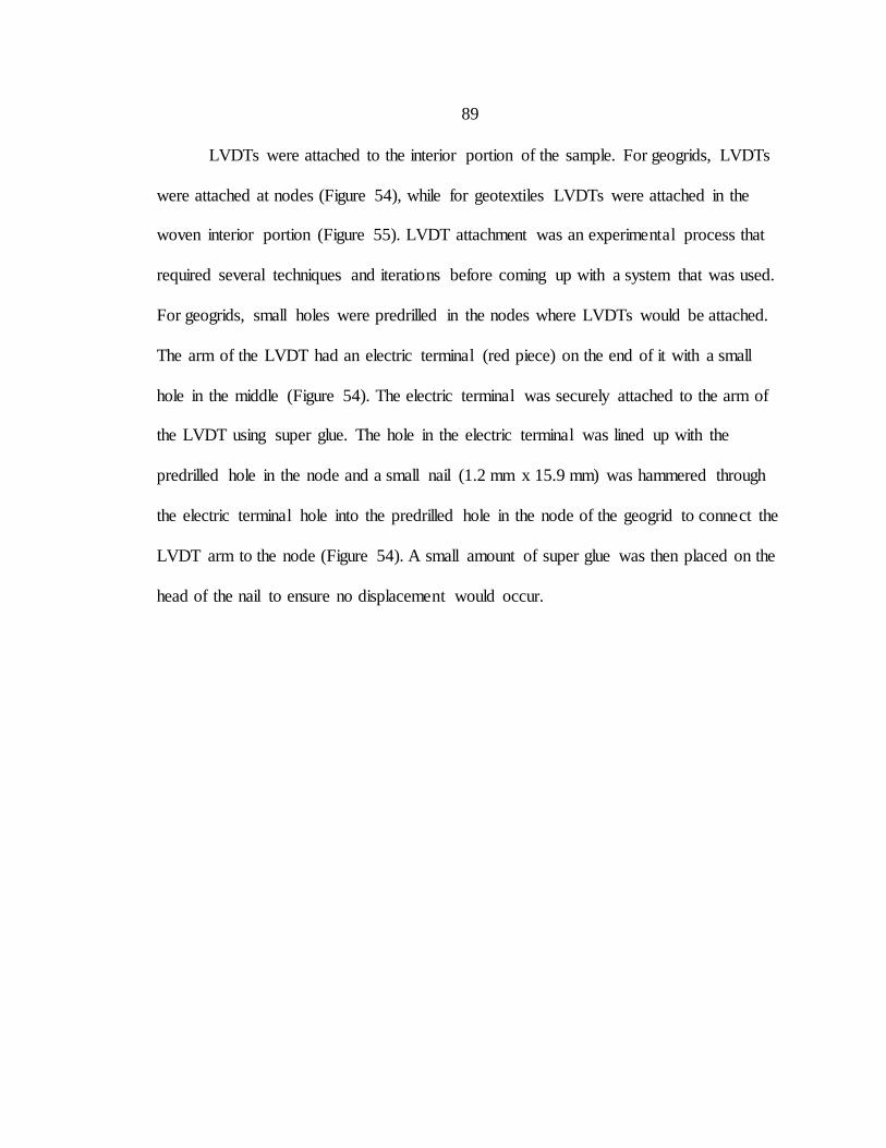
89
LVDTs were attached to the interior portion of the sample. For geogrids, LVDTs
were attached at nodes (Figure 54), while for geotextiles LVDTs were attached in the
woven interior portion (Figure 55). LVDT attachment was an experimental process that
required several techniques and iterations before coming up with a system that was used.
For geogrids, small holes were predrilled in the nodes where LVDTs would be attached.
The arm of the LVDT had an electric terminal (red piece) on the end of it with a small
hole in the middle (Figure 54). The electric terminal was securely attached to the arm of
the LVDT using super glue. The hole in the electric terminal was lined up with the
predrilled hole in the node and a small nail (1.2 mm x 15.9 mm) was hammered through
the electric terminal hole into the predrilled hole in the node of the geogrid to connect the
LVDT arm to the node (Figure 54). A small amount of super glue was then placed on the
head of the nail to ensure no displacement would occur.
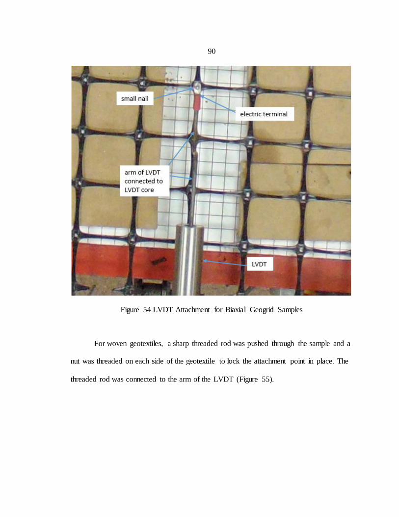
90
Figure 54 LVDT Attachment for Biaxial Geogrid Samples
For woven geotextiles, a sharp threaded rod was pushed through the sample and a
nut was threaded on each side of the geotextile to lock the attachment point in place. The
threaded rod was connected to the arm of the LVDT (Figure 55).
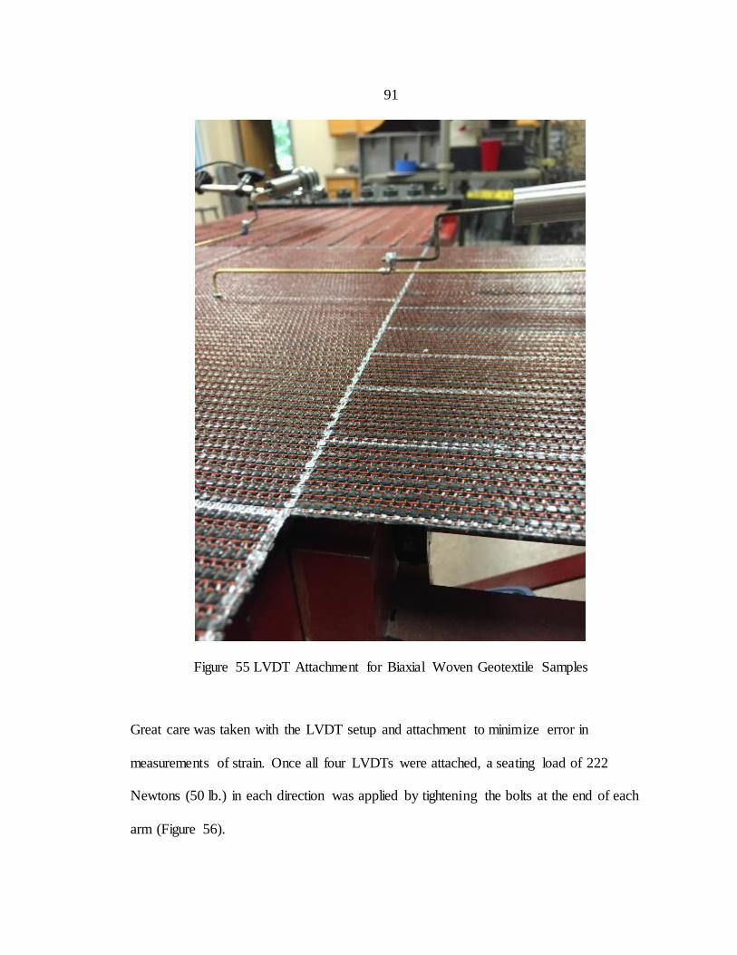
91
Figure 55 LVDT Attachment for Biaxial Woven Geotextile Samples
Great care was taken with the LVDT setup and attachment to minimize error in
measurements of strain. Once all four LVDTs were attached, a seating load of 222
Newtons (50 lb.) in each direction was applied by tightening the bolts at the end of each
arm (Figure 56).

92
Figure 56 Biaxial Testing Device, Bolt for Applying Seating Load
When applying the seating load, the material was again carefully centered on the
device. Wooden blocks were placed underneath the interior portion of the sample to
minimize any displacement in the z-direction when tensioned (Figure 52). Once the
seating load was applied, a gauge length in both directions was measured from the center
lines of the nails used to attach the LVDT arm to the geogrid node. For geotextiles the
gauge length was measured from centerline to centerline of the threaded rod. The sample
width for geogrids was determined as outlined by ASTM D7556 and discussed in the
uniaxial testing section (Figure 15). For geotextiles, the width was just simply measured
93
as the width of the sample. The LVDTs were then adjusted such that the inner core was
parallel with the outer core and parallel with the geosynthetic material. It was then double
checked that the seating load was still at 222 Newtons (50 lbs) before the test was started.
Recommendations for specimen dimensions of biaxial samples was examined by
Bridgens and Gosling (2003) and MSAJ (1995) for structural membranes in the
Literature Review section. The gauge points must be sufficiently far from edge of the
interior portion such that any effects from the grips are not noticed and the
instrumentation is placed within the zone of uniform stress and strain as observed by
Krause and Bartolotta (2001) and Bridgens and Gosling (2003). Bridgens and Gosling
(2003) and MSAJ (1995) both used smaller biaxial testing devices with smaller overall
sample dimensions than was used for this thesis. The ratio of sample width to
recommended gauge length for samples tested by Bridgens and Gosling (2003) was 2/3.
The Japanese testing standard recommended sample widths of 48 cm or more and used
gauge lengths ranging from 20 to 80 mm. McGown et al. (2004) conducted biaxial tests
on geogrids using cruciform shaped samples with central areas of 100 to 220 mm square
with 5 ribs in each direction but measured displacement using photogrammetric
techniques. The biaxial geogrids tested had rectangular apertures, thus the XMD and MD
directions had slightly different sample widths and gauge lengths. The samples were
always symmetric with respect to each direction and the same sample size was used for
each given material for all trials and all modes of loading. Sample dimensions used were
decided based upon the available literature and the size and layout of the available biaxial
94
testing device. Typical interior sample widths ranged from 365 mm to 422 mm and gauge
lengths ranged from 127 mm to 178 mm.
Testing Procedure
Biaxial tests were run with the motor set at a speed of approximately 3450
rotations per minute, which corresponds to a displacement of the load plate of 8.76 cm
(3.45 inches) per minute. Initially it was desired to use ASTMD D7556 as a guideline for
strain rate, but the biaxial device was not capable of producing a strain rate that satisfied
this standard. The strain rate as outlined in ASTM D7556 should be 10 ± 3 % per minute.
The motor was run at its maximum speed which produced strain rates of approximately 5
% per minute. Measured strain rates for trial biaxial tests are listed later in this chapter in
Table 30.
A laptop computer and data acquisition system were connected to the testing
device to record real time values of load and displacement in both directions. Using the
measured gauge lengths in both directions, displacements that correspond to strains of
0.5, 1.0, 1.5, 2.0, 3.0 and 4.0 % were calculated for both directions. The motor was then
switched on and run until the material reached the displacement corresponding to a strain
of 0.5 %. The motor was then shut off and a timer for 20 minutes was started. This
process was continued for all permanent strain limits. This procedure was used for all
materials tested and for all modes of loading.
The procedure described had some inherent human error with reaching the
permanent strain limits. To reach the permanent strain limits, the motor had to be stopped
95
manually at the desired displacement. This was difficult to do with high precision
because once the switch for the motor was turned off, the motor would continue to spin
while slowing down. This deceleration period would cause more displacement in the
material. After lots of practice, this process was not very difficult, but it was still
impossible to have identical values of permanent strain limits for each material and each
trial. The permanent strain values were approximated as best as possible and recorded so
this was not a large issue. Another problem encountered with the testing device was its
inability to load materials to 3.0 and 4.0 % permanent strain for some of the stiffer
geosynthetics tested. The motor did not have the power to load some of these materials to
the upper strain limits, and the load cell reached its capacity of 8896 N (2000 lbs) for
some materials. Tests were run to the highest level of permanent strain that was attainable
for materials where these limitations were encountered. It was discovered that if the
motor speed was slowed down after initially loading the material at full speed, the motor
was capable of applying a little more displacement. When possible, this was done to load
the material to one more strain limit.
Biaxial Testing Results
The results from Geogrid A will be presented in this section because the greatest
number of trials for each mode were performed on this material. The results obtained for
this material and the analysis process that follows were performed for all materials tested.
The load per unit width versus strain plot for a mode 1 loading is shown in Figure 57.
The X-direction is always the XMD or 1-direction and the Y-Direction is always the MD
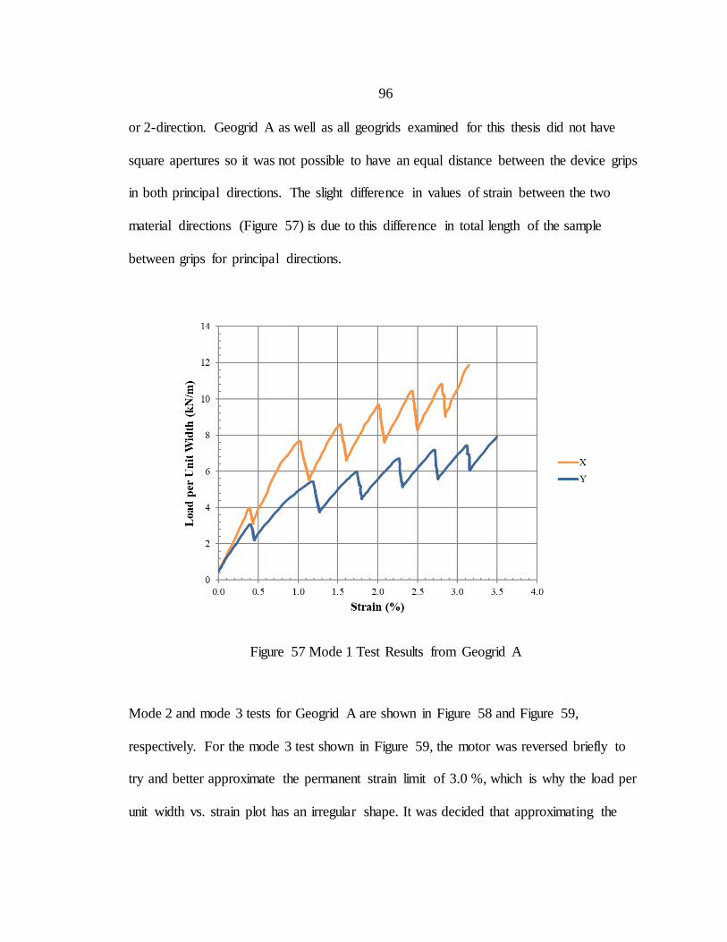
96
or 2-direction. Geogrid A as well as all geogrids examined for this thesis did not have
square apertures so it was not possible to have an equal distance between the device grips
in both principal directions. The slight difference in values of strain between the two
material directions (Figure 57) is due to this difference in total length of the sample
between grips for principal directions.
Figure 57 Mode 1 Test Results from Geogrid A
Mode 2 and mode 3 tests for Geogrid A are shown in Figure 58 and Figure 59,
respectively. For the mode 3 test shown in Figure 59, the motor was reversed briefly to
try and better approximate the permanent strain limit of 3.0 %, which is why the load per
unit width vs. strain plot has an irregular shape. It was decided that approximating the
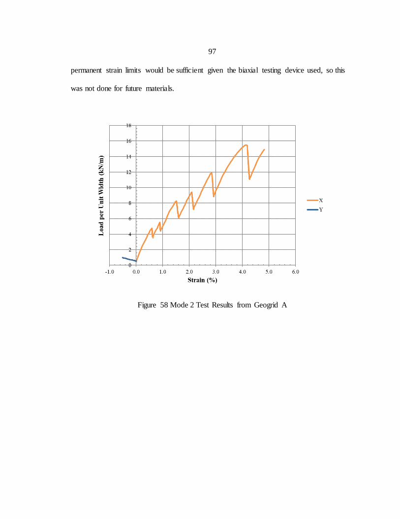
97
permanent strain limits would be sufficient given the biaxial testing device used, so this
was not done for future materials.
Figure 58 Mode 2 Test Results from Geogrid A
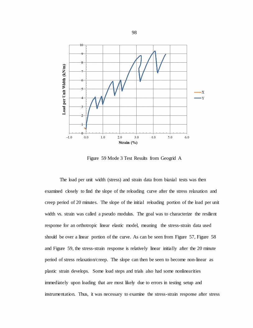
98
Figure 59 Mode 3 Test Results from Geogrid A
The load per unit width (stress) and strain data from biaxial tests was then
examined closely to find the slope of the reloading curve after the stress relaxation and
creep period of 20 minutes. The slope of the initial reloading portion of the load per unit
width vs. strain was called a pseudo modulus. The goal was to characterize the resilient
response for an orthotropic linear elastic model, meaning the stress-strain data used
should be over a linear portion of the curve. As can be seen from Figure 57, Figure 58
and Figure 59, the stress-strain response is relatively linear initially after the 20 minute
period of stress relaxation/creep. The slope can then be seen to become non-linear as
plastic strain develops. Some load steps and trials also had some nonlinearities
immediately upon loading that are most likely due to errors in testing setup and
instrumentation. Thus, it was necessary to examine the stress-strain response after stress
99
relaxation/creep on a case by case basis to ensure the response was linear and
representative of the resilient material response. The pseudo modulus was calculated
using a best fit linear trendline of the stress/strain data after each stress relaxation/creep
period as shown in Figure 60. The stress/strain interval selected for calculation of the
pseudo modulus varied slightly from trial to trial in order to use the most linear portion of
the reloading curve after stress relaxation/creep.
As mentioned in the testing procedure section, the stiffness of geosynthetics is
dependent on strain rate (Perkins, 2000). The strain rate outlined in ASTM D7556 was
not achievable with the biaxial testing device used for this testing. The strain rates for the
data used for calculation of the pseudo modulus is shown in Table 30 for all six trials of
mode 1 loading on Geogrid A. The strain rates vary between 2.99 and 7.59 % / minute
and are almost all below the minimum value of 7.0 % per minute as outlined in ASTM
D7556. The variability is attributed to several factors including the method in which
pseudo modulus was calculated and imperfections in testing setup, instrumentation and
the testing device. The electric motor used to control displacement (strain) has a short
acceleration period and does not immediately rotate at its maximum speed. During this
short acceleration period, the material does not experience a constant rate of strain. Since
the pseudo modulus was calculated from the initial loading this means the strain rate is
increasing then constant in the region of loading used for calculation of pseudo modulus.
Since the pseudo modulus was calculated on a case by case basis, the strain interval was
not always equal, meaning the strain rates shown in Table 30 should be expected to be
variable.
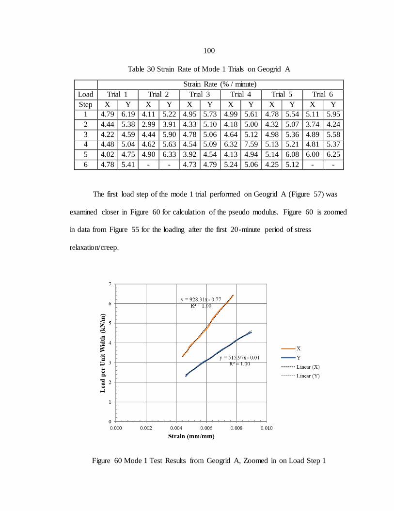
100
Table 30 Strain Rate of Mode 1 Trials on Geogrid A
Strain Rate (% / minute)
Load Trial 1 Trial 2 Trial 3 Trial 4 Trial 5 Trial 6
Step X Y X Y X Y X Y X Y X Y
1 4.79 6.19 4.11 5.22 4.95 5.73 4.99 5.61 4.78 5.54 5.11 5.95
2 4.44 5.38 2.99 3.91 4.33 5.10 4.18 5.00 4.32 5.07 3.74 4.24
3 4.22 4.59 4.44 5.90 4.78 5.06 4.64 5.12 4.98 5.36 4.89 5.58
4 4.48 5.04 4.62 5.63 4.54 5.09 6.32 7.59 5.13 5.21 4.81 5.37
5 4.02 4.75 4.90 6.33 3.92 4.54 4.13 4.94 5.14 6.08 6.00 6.25
6 4.78 5.41 - - 4.73 4.79 5.24 5.06 4.25 5.12 - -
The first load step of the mode 1 trial performed on Geogrid A (Figure 57) was
examined closer in Figure 60 for calculation of the pseudo modulus. Figure 60 is zoomed
in data from Figure 55 for the loading after the first 20-minute period of stress
relaxation/creep.
Figure 60 Mode 1 Test Results from Geogrid A, Zoomed in on Load Step 1
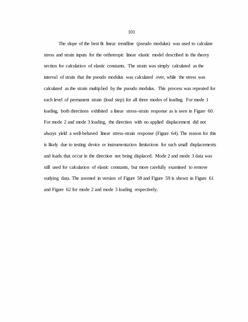
101
The slope of the best fit linear trendline (pseudo modulus) was used to calculate
stress and strain inputs for the orthotropic linear elastic model described in the theory
section for calculation of elastic constants. The strain was simply calculated as the
interval of strain that the pseudo modulus was calculated over, while the stress was
calculated as the strain multiplied by the pseudo modulus. This process was repeated for
each level of permanent strain (load step) for all three modes of loading. For mode 1
loading, both directions exhibited a linear stress-strain response as is seen in Figure 60.
For mode 2 and mode 3 loading, the direction with no applied displacement did not
always yield a well-behaved linear stress-strain response (Figure 64). The reason for this
is likely due to testing device or instrumentation limitations for such small displacements
and loads that occur in the direction not being displaced. Mode 2 and mode 3 data was
still used for calculation of elastic constants, but more carefully examined to remove
outlying data. The zoomed in version of Figure 58 and Figure 59 is shown in Figure 61
and Figure 62 for mode 2 and mode 3 loading respectively.
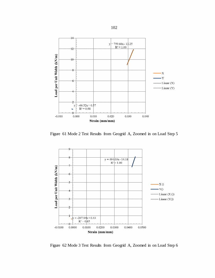
102
Figure 61 Mode 2 Test Results from Geogrid A, Zoomed in on Load Step 5
Figure 62 Mode 3 Test Results from Geogrid A, Zoomed in on Load Step 6
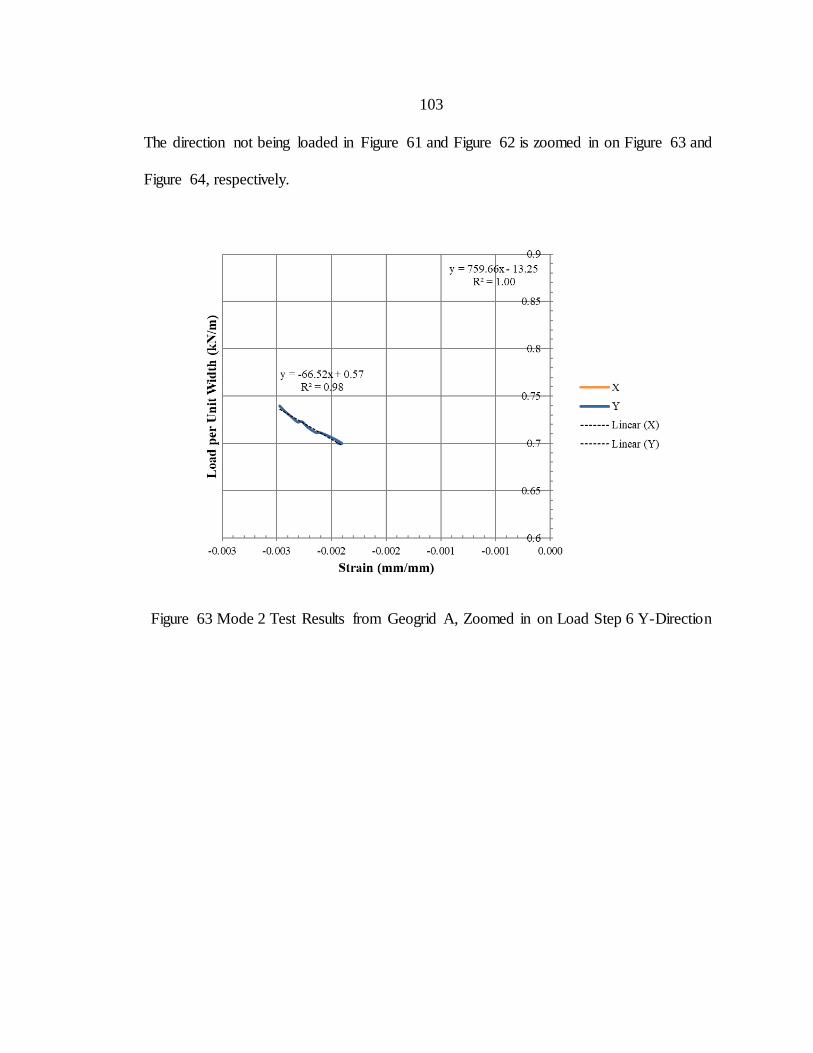
103
The direction not being loaded in Figure 61 and Figure 62 is zoomed in on Figure 63 and
Figure 64, respectively.
Figure 63 Mode 2 Test Results from Geogrid A, Zoomed in on Load Step 6 Y-Direction
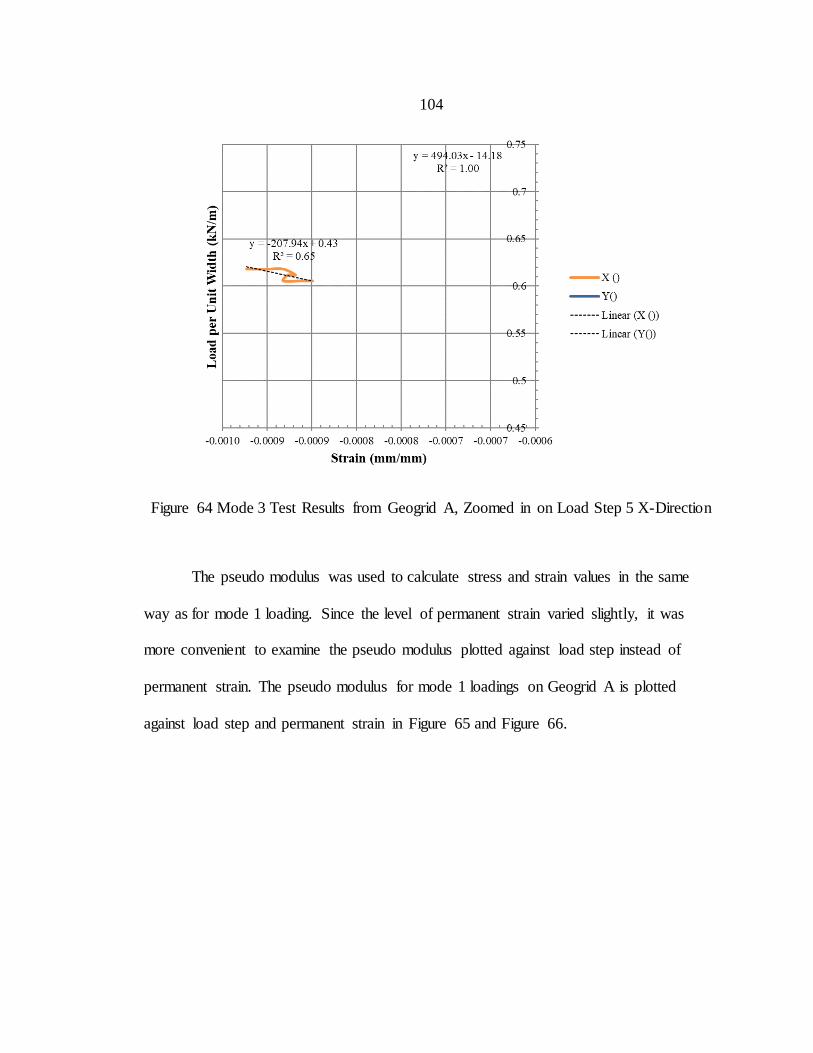
104
Figure 64 Mode 3 Test Results from Geogrid A, Zoomed in on Load Step 5 X-Direction
The pseudo modulus was used to calculate stress and strain values in the same
way as for mode 1 loading. Since the level of permanent strain varied slightly, it was
more convenient to examine the pseudo modulus plotted against load step instead of
permanent strain. The pseudo modulus for mode 1 loadings on Geogrid A is plotted
against load step and permanent strain in Figure 65 and Figure 66.
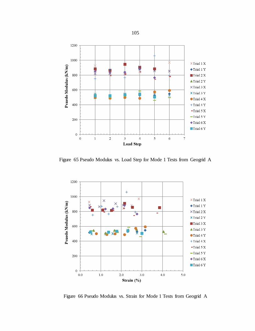
105
Figure 65 Pseudo Modulus vs. Load Step for Mode 1 Tests from Geogrid A
Figure 66 Pseudo Modulus vs. Strain for Mode 1 Tests from Geogrid A
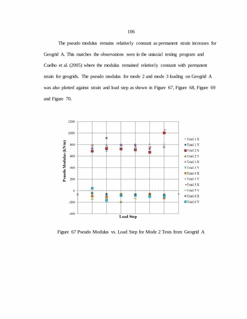
106
The pseudo modulus remains relatively constant as permanent strain increases for
Geogrid A. This matches the observations seen in the uniaxial testing program and
Cuelho et al. (2005) where the modulus remained relatively constant with permanent
strain for geogrids. The pseudo modulus for mode 2 and mode 3 loading on Geogrid A
was also plotted against strain and load step as shown in Figure 67, Figure 68, Figure 69
and Figure 70.
Figure 67 Pseudo Modulus vs. Load Step for Mode 2 Tests from Geogrid A
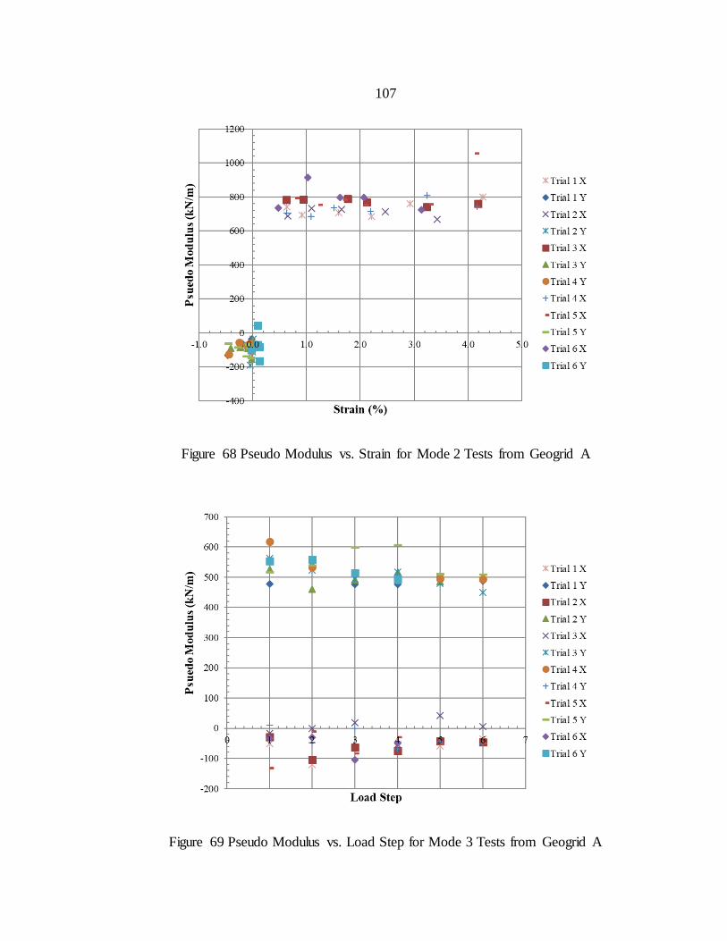
107
Figure 68 Pseudo Modulus vs. Strain for Mode 2 Tests from Geogrid A
Figure 69 Pseudo Modulus vs. Load Step for Mode 3 Tests from Geogrid A
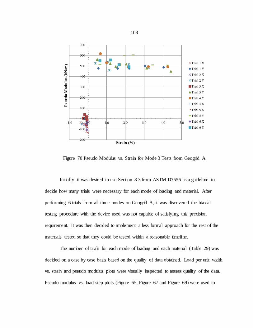
108
Figure 70 Pseudo Modulus vs. Strain for Mode 3 Tests from Geogrid A
Initially it was desired to use Section 8.3 from ASTM D7556 as a guideline to
decide how many trials were necessary for each mode of loading and material. After
performing 6 trials from all three modes on Geogrid A, it was discovered the biaxial
testing procedure with the device used was not capable of satisfying this precision
requirement. It was then decided to implement a less formal approach for the rest of the
materials tested so that they could be tested within a reasonable timeline.
The number of trials for each mode of loading and each material (Table 29) was
decided on a case by case basis based on the quality of data obtained. Load per unit width
vs. strain and pseudo modulus plots were visually inspected to assess quality of the data.
Pseudo modulus vs. load step plots (Figure 65, Figure 67 and Figure 69) were used to
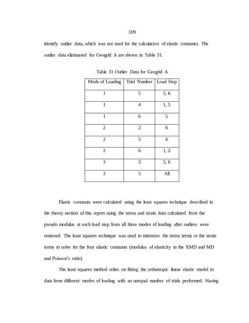
109
identify outlier data, which was not used for the calculation of elastic constants. The
outlier data eliminated for Geogrid A are shown in Table 31.
Table 31 Outlier Data for Geogrid A
Mode of Loading Trial Number Load Step
1 5 5, 6
1 4 1, 5
1 6 5
2 2 6
2 5 6
2 6 1, 2
3 3 5, 6
3 5 All
Elastic constants were calculated using the least squares technique described in
the theory section of this report using the stress and strain data calculated from the
pseudo modulus at each load step from all three modes of loading after outliers were
removed. The least squares technique was used to minimize the stress terms or the strain
terms to solve for the four elastic constants (modulus of elasticity in the XMD and MD
and Poisson’s ratio).
The least squares method relies on fitting the orthotropic linear elastic model to
data from different modes of loading with an unequal number of trials performed. Having
110
a different number of trials for each mode of loading biases the results of the least squares
regression to those modes with a higher number of trials, which undermines the goal of
the method. To eliminate this bias, a single data set was created for each mode of loading
and load step. This was accomplished by first taking an average of the pseudo modulus
from all trials at each load step and for each mode of loading. The ratio of strain in the x-
direction (1-direction) and strain in the y-direction (2-direction) was then taken for all
trials at each load step and each mode of loading. The strain ratio was then averaged for
all trials for each load step and mode of loading. This resulted in a single value for
average strain ratio and average pseudo modulus for each load step and mode of loading.
It was also recognized that if the stress/strain data used for calculation of elastic constants
was not over an equal interval of stress or strain this would create a slight bias. The
Japanese Testing Standard recommended that stress strain data over an equal load
interval be used for the determination of elastic constants. For this thesis it was decided
that using an equal strain interval of 0.2 % was appropriate because this is what was done
for determination of uniaxial properties.
A stress-strain data set was created by assigning an arbitrary value of strain of 0.2
% to the strain value in the direction being loaded (x-direction for mode 1 (could also
choose y-direction for mode 1), x-direction for mode 2, y-direction for mode 3). The
strain in the other direction was then calculated based upon the average strain ratio for
that given load step and mode of loading. The stress values were calculated using the
average pseudo modulus multiplied by the strain for the given load step and mode of
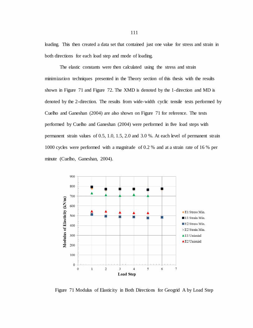
111
loading. This then created a data set that contained just one value for stress and strain in
both directions for each load step and mode of loading.
The elastic constants were then calculated using the stress and strain
minimization techniques presented in the Theory section of this thesis with the results
shown in Figure 71 and Figure 72. The XMD is denoted by the 1-direction and MD is
denoted by the 2-direction. The results from wide-width cyclic tensile tests performed by
Cuelho and Ganeshan (2004) are also shown on Figure 71 for reference. The tests
performed by Cuelho and Ganeshan (2004) were performed in five load steps with
permanent strain values of 0.5, 1.0, 1.5, 2.0 and 3.0 %. At each level of permanent strain
1000 cycles were performed with a magnitude of 0.2 % and at a strain rate of 16 % per
minute (Cuelho, Ganeshan, 2004).
Figure 71 Modulus of Elasticity in Both Directions for Geogrid A by Load Step

112
Figure 72 Poisson’s Ratio in Both Directions for Geogrid A by Load Step
Observing Figure 71, the uniaxial modulus in the MD is slightly lower than the
biaxial modulus, while the opposite is true for the XMD. It is important to remember that
the biaxial modulus values are not expected to match the uniaxial values because they are
from a different testing procedure with different cycle/hold times, strain rates and
boundary conditions. The comparison between uniaxial and biaxial results was made only
to confirm that the modulus of elasticity values being calculated from biaxial tests were
reasonable. The increased stiffness observed in the XMD from biaxial tests in
comparison to uniaxial could be due to the behavior of the junctions of geogrids under
biaxial loading in comparison to uniaxial loading as discussed in the literature review and
observed by McGown et al. (2004).
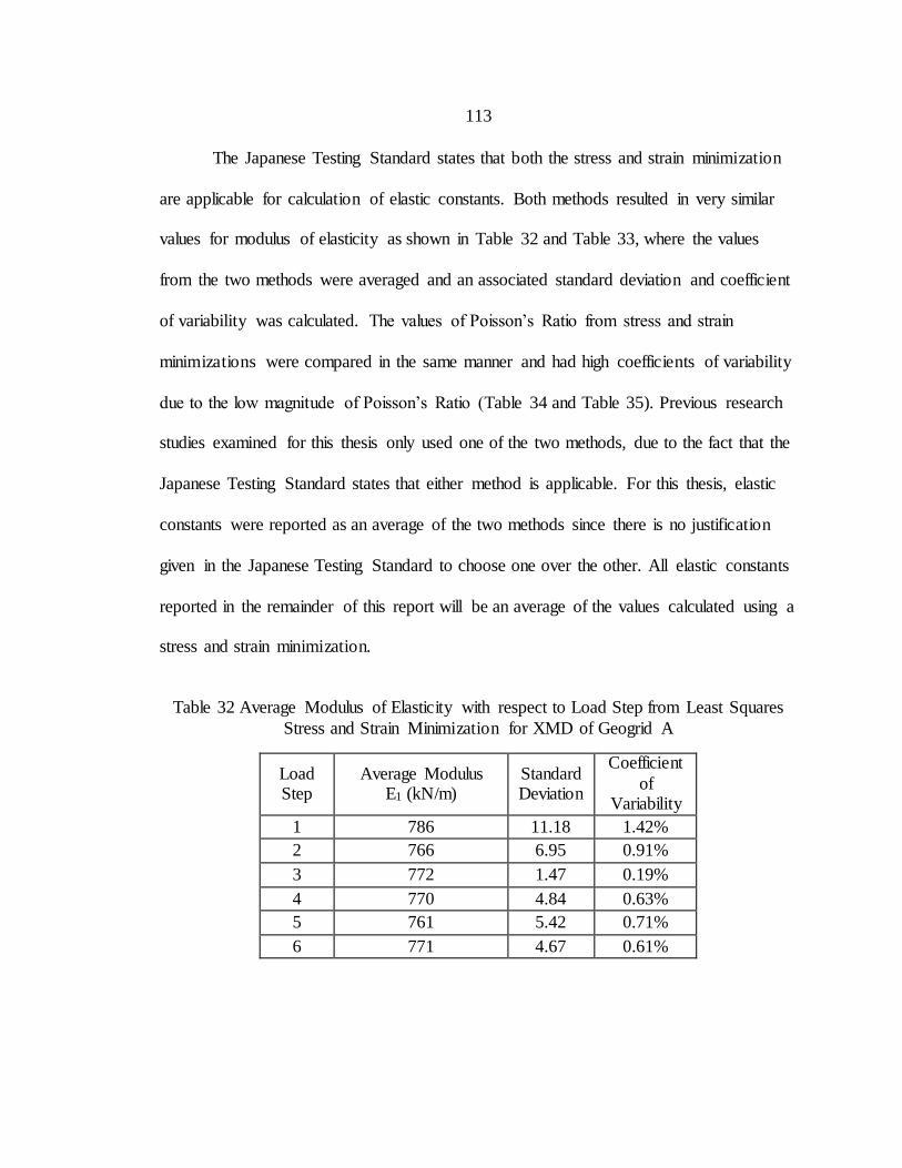
113
The Japanese Testing Standard states that both the stress and strain minimization
are applicable for calculation of elastic constants. Both methods resulted in very similar
values for modulus of elasticity as shown in Table 32 and Table 33, where the values
from the two methods were averaged and an associated standard deviation and coefficient
of variability was calculated. The values of Poisson’s Ratio from stress and strain
minimizations were compared in the same manner and had high coefficients of variability
due to the low magnitude of Poisson’s Ratio (Table 34 and Table 35). Previous research
studies examined for this thesis only used one of the two methods, due to the fact that the
Japanese Testing Standard states that either method is applicable. For this thesis, elastic
constants were reported as an average of the two methods since there is no justification
given in the Japanese Testing Standard to choose one over the other. All elastic constants
reported in the remainder of this report will be an average of the values calculated using a
stress and strain minimization.
Table 32 Average Modulus of Elasticity with respect to Load Step from Least Squares
Stress and Strain Minimization for XMD of Geogrid A
Load Step
Average Modulus E1 (kN/m)
Standard Deviation
Coefficient
of Variability
1 786 11.18 1.42%
2 766 6.95 0.91%
3 772 1.47 0.19%
4 770 4.84 0.63%
5 761 5.42 0.71%
6 771 4.67 0.61%
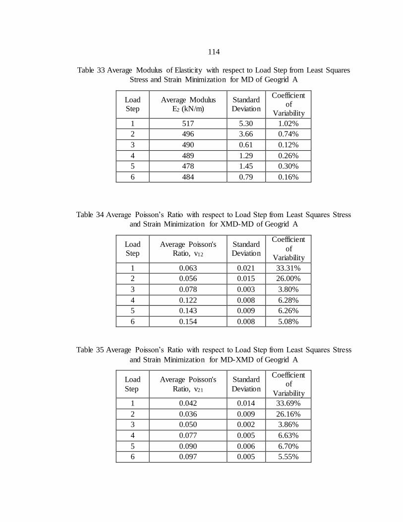
114
Table 33 Average Modulus of Elasticity with respect to Load Step from Least Squares
Stress and Strain Minimization for MD of Geogrid A
Load Step
Average Modulus E2 (kN/m)
Standard Deviation
Coefficient of
Variability
1 517 5.30 1.02%
2 496 3.66 0.74%
3 490 0.61 0.12%
4 489 1.29 0.26%
5 478 1.45 0.30%
6 484 0.79 0.16%
Table 34 Average Poisson’s Ratio with respect to Load Step from Least Squares Stress
and Strain Minimization for XMD-MD of Geogrid A
Load Step
Average Poisson's Ratio, v12
Standard Deviation
Coefficient
of Variability
1 0.063 0.021 33.31%
2 0.056 0.015 26.00%
3 0.078 0.003 3.80%
4 0.122 0.008 6.28%
5 0.143 0.009 6.26%
6 0.154 0.008 5.08%
Table 35 Average Poisson’s Ratio with respect to Load Step from Least Squares Stress
and Strain Minimization for MD-XMD of Geogrid A
Load
Step
Average Poisson's
Ratio, v21
Standard
Deviation
Coefficient of
Variability
1 0.042 0.014 33.69%
2 0.036 0.009 26.16%
3 0.050 0.002 3.86%
4 0.077 0.005 6.63%
5 0.090 0.006 6.70%
6 0.097 0.005 5.55%
115
To examine how well the elastic constants fit the data measured from biaxial
tension tests, the stress values in both direction were calculated using Equations (11) and
(12) from the Theory section and shown again below. The stress values were calculated
using the measured strain from biaxial tests and the elastic constants for each load step
from Table 32, Table 33, Table 34 and Table 35. These calculated stress values were then
compared to the measured stress values from biaxial tension tests. The calculated and
measured stress values in both directions from all load steps for all trials from all three
modes of loading after outliers were removed are shown on Figure 73.
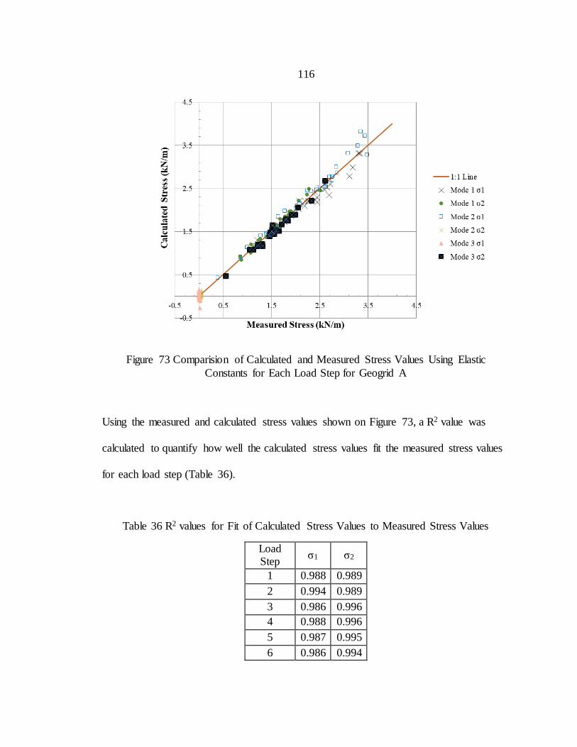
116
Figure 73 Comparision of Calculated and Measured Stress Values Using Elastic
Constants for Each Load Step for Geogrid A
Using the measured and calculated stress values shown on Figure 73, a R2 value was
calculated to quantify how well the calculated stress values fit the measured stress values
for each load step (Table 36).
Table 36 R2 values for Fit of Calculated Stress Values to Measured Stress Values
Load Step
σ1 σ2
1 0.988 0.989
2 0.994 0.989
3 0.986 0.996
4 0.988 0.996
5 0.987 0.995
6 0.986 0.994
117
The comparison shown on Figure 73 with the associated R2 values (Table 36),
shows that the elastic constants used (Table 32, Table 33, Table 34 and Table 35) to
describe the resilient response of Geogrid A fit the measured data. The direction with
applied displacement (σ1 and σ2 for mode 1, σ1 for mode 2 and σ2 for mode 3) is
described very well by the elastic constants as shown by how similar the calculated stress
and measured stress values are on Figure 73. The direction with no applied displacement
(σ2 for mode 2 and σ1 mode 3) has very low stress and strain values and the measured
stress values were more variable than those in the direction being loaded. These low and
more variable measured stress values lead to slightly larger differences between the
calculated and measured stress values for σ2 values from mode 2 and σ1 values from mode
3 loading. Overall the high correlation between measured and calculated stress values
(Table 36) combined with the fact that the modulus values are in the range of values
calculated previously using uniaxial tests gives confidence to these values for elastic
constants.
Observing Figure 71 and Figure 72, it was noted that the modulus of elasticity
values appear to remain relatively constant with increasing levels of permanent strain
(load step). This is encouraging as all previously calculated measures of stiffness for
geogrids have shown little change in stiffness with increasing permanent strain. When
examined closely, the modulus of elasticity in both directions does slightly decrease with
load step (Table 32 and Table 33), while Poisson’s Ratio slightly increases (Table 34 and
Table 35). The slight decrease in modulus as permanent strain increases was also
observed by Cuelho and Ganeshan (2004) for Geogrid A.
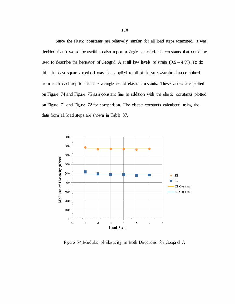
118
Since the elastic constants are relatively similar for all load steps examined, it was
decided that it would be useful to also report a single set of elastic constants that could be
used to describe the behavior of Geogrid A at all low levels of strain (0.5 – 4 %). To do
this, the least squares method was then applied to all of the stress/strain data combined
from each load step to calculate a single set of elastic constants. These values are plotted
on Figure 74 and Figure 75 as a constant line in addition with the elastic constants plotted
on Figure 71 and Figure 72 for comparison. The elastic constants calculated using the
data from all load steps are shown in Table 37.
Figure 74 Modulus of Elasticity in Both Directions for Geogrid A
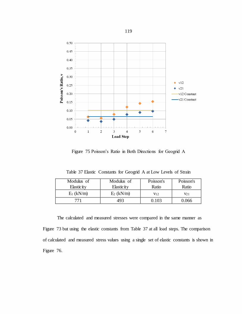
119
Figure 75 Poisson’s Ratio in Both Directions for Geogrid A
Table 37 Elastic Constants for Geogrid A at Low Levels of Strain
Modulus of
Elasticity
Modulus of
Elasticity
Poisson's
Ratio
Poisson's
Ratio
E1 (kN/m) E2 (kN/m) v12 v21
771 493 0.103 0.066
The calculated and measured stresses were compared in the same manner as
Figure 73 but using the elastic constants from Table 37 at all load steps. The comparison
of calculated and measured stress values using a single set of elastic constants is shown in
Figure 76.
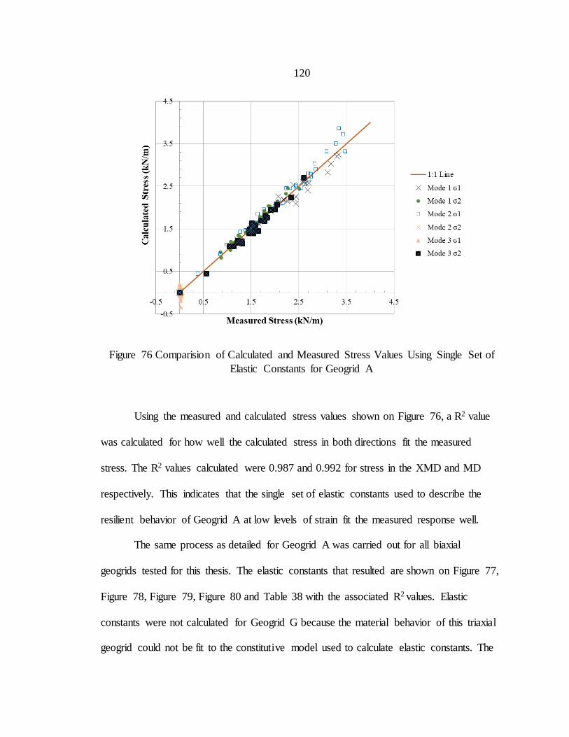
120
Figure 76 Comparision of Calculated and Measured Stress Values Using Single Set of
Elastic Constants for Geogrid A
Using the measured and calculated stress values shown on Figure 76, a R2 value
was calculated for how well the calculated stress in both directions fit the measured
stress. The R2 values calculated were 0.987 and 0.992 for stress in the XMD and MD
respectively. This indicates that the single set of elastic constants used to describe the
resilient behavior of Geogrid A at low levels of strain fit the measured response well.
The same process as detailed for Geogrid A was carried out for all biaxial
geogrids tested for this thesis. The elastic constants that resulted are shown on Figure 77,
Figure 78, Figure 79, Figure 80 and Table 38 with the associated R2 values. Elastic
constants were not calculated for Geogrid G because the material behavior of this triaxial
geogrid could not be fit to the constitutive model used to calculate elastic constants. The
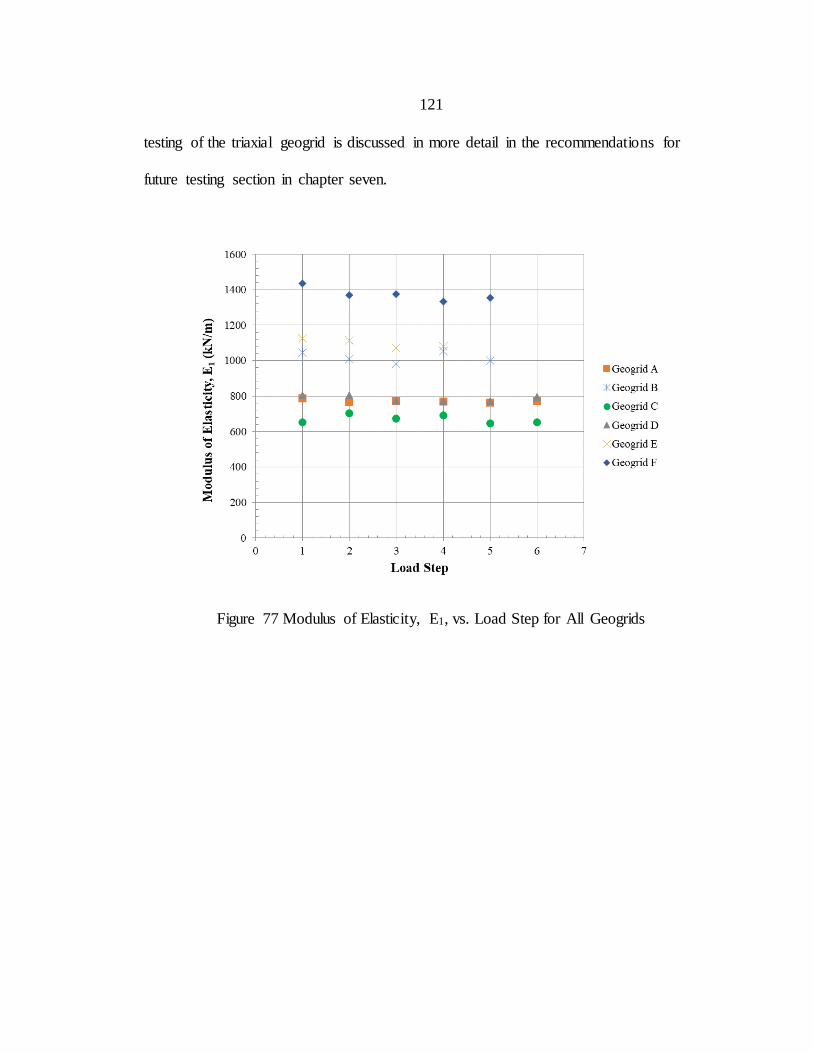
121
testing of the triaxial geogrid is discussed in more detail in the recommendations for
future testing section in chapter seven.
Figure 77 Modulus of Elasticity, E1, vs. Load Step for All Geogrids
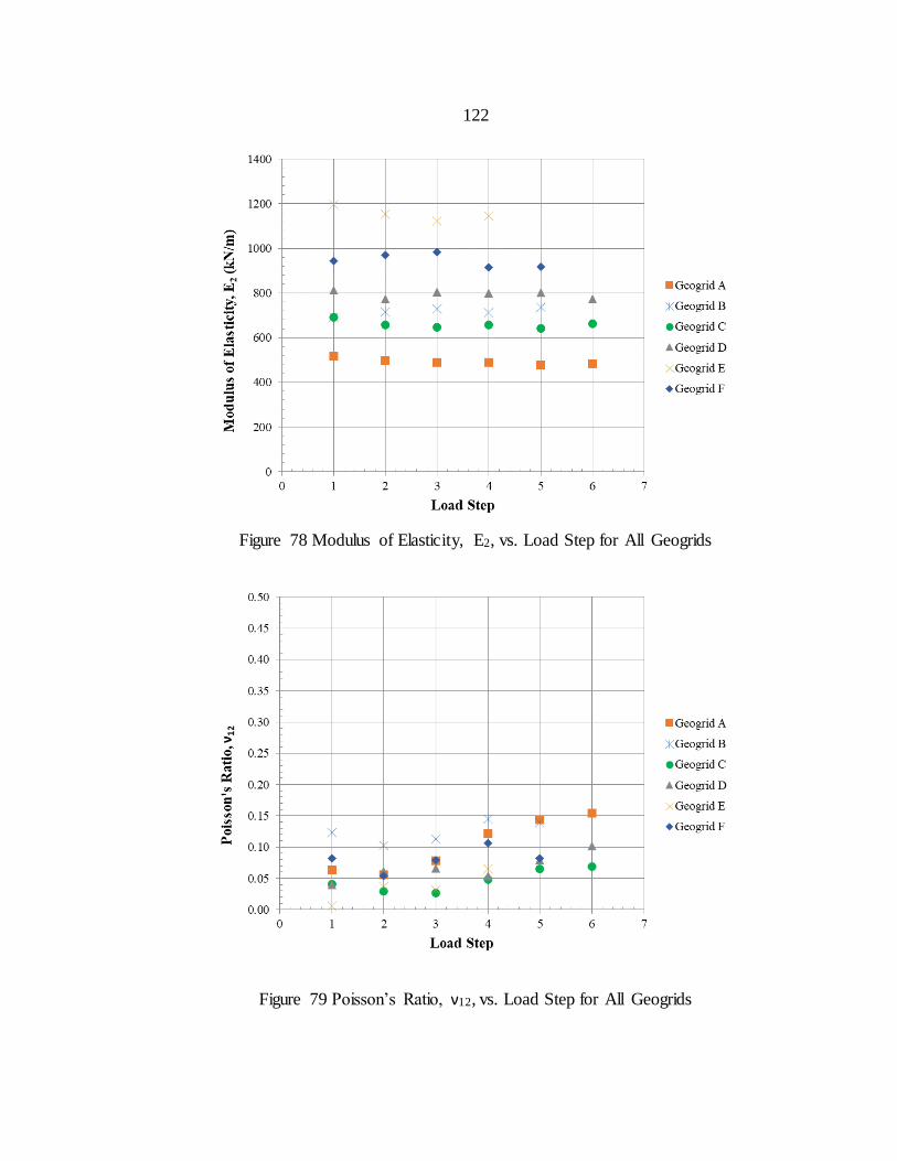
122
Figure 78 Modulus of Elasticity, E2, vs. Load Step for All Geogrids
Figure 79 Poisson’s Ratio, ν12, vs. Load Step for All Geogrids
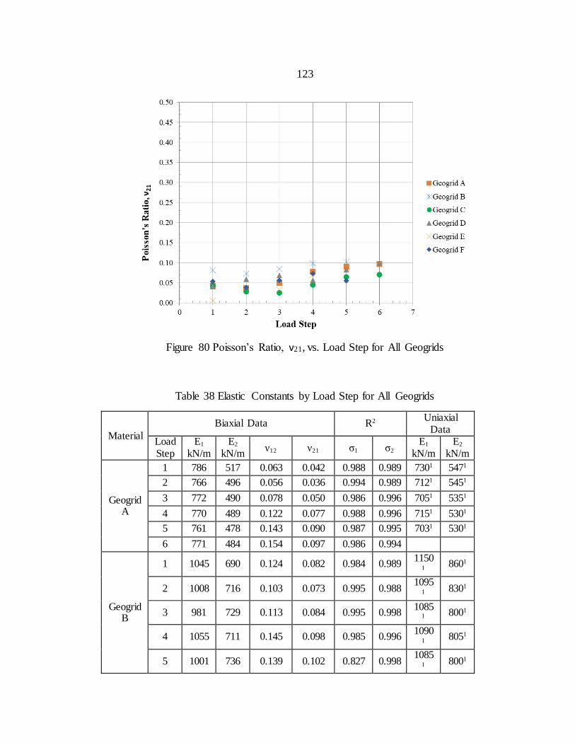
123
Figure 80 Poisson’s Ratio, ν21, vs. Load Step for All Geogrids
Table 38 Elastic Constants by Load Step for All Geogrids
Material
Biaxial Data R2 Uniaxial
Data Load Step
E1 kN/m
E2 kN/m
ν12 ν21 σ1 σ2 E1
kN/m E2
kN/m
Geogrid A
1 786 517 0.063 0.042 0.988 0.989 7301 5471
2 766 496 0.056 0.036 0.994 0.989 7121 5451
3 772 490 0.078 0.050 0.986 0.996 7051 5351
4 770 489 0.122 0.077 0.988 0.996 7151 5301
5 761 478 0.143 0.090 0.987 0.995 7031 5301
6 771 484 0.154 0.097 0.986 0.994
Geogrid B
1 1045 690 0.124 0.082 0.984 0.989 1150
1 8601
2 1008 716 0.103 0.073 0.995 0.988 1095
1 8301
3 981 729 0.113 0.084 0.995 0.998 1085
1 8001
4 1055 711 0.145 0.098 0.985 0.996 1090
1 8051
5 1001 736 0.139 0.102 0.827 0.998 1085
1 8001
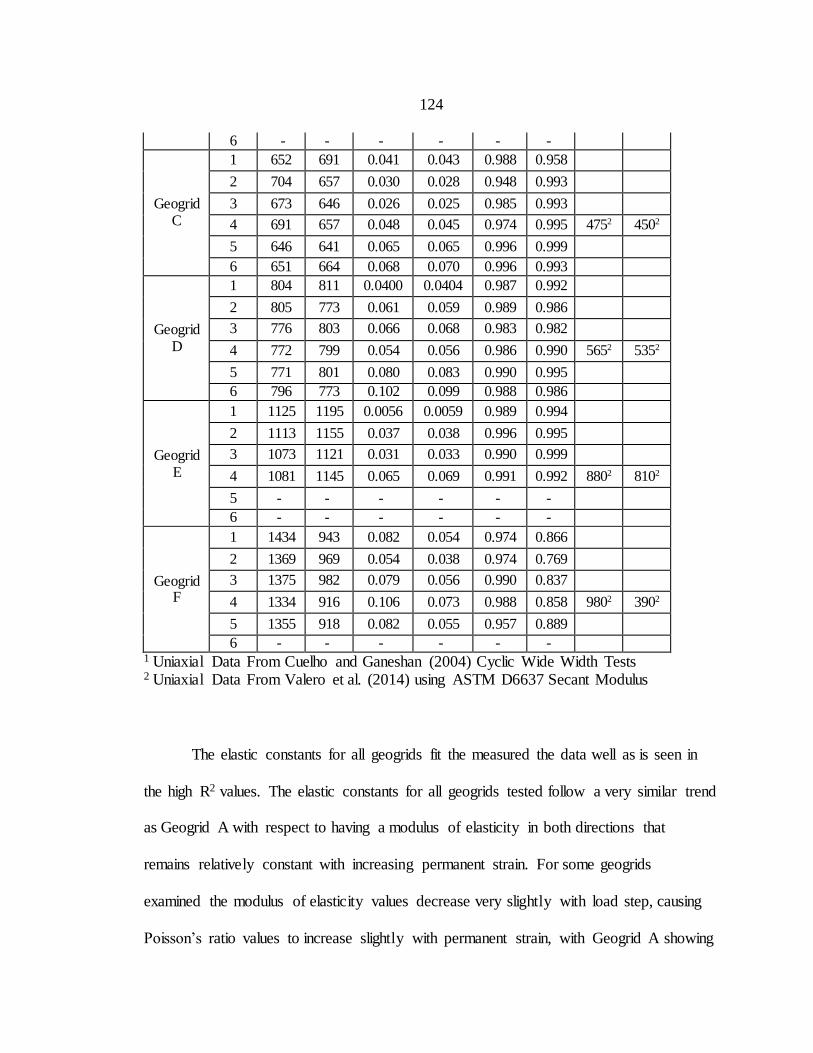
124
6 - - - - - -
Geogrid C
1 652 691 0.041 0.043 0.988 0.958
2 704 657 0.030 0.028 0.948 0.993
3 673 646 0.026 0.025 0.985 0.993
4 691 657 0.048 0.045 0.974 0.995 4752 4502
5 646 641 0.065 0.065 0.996 0.999
6 651 664 0.068 0.070 0.996 0.993
Geogrid D
1 804 811 0.0400 0.0404 0.987 0.992
2 805 773 0.061 0.059 0.989 0.986
3 776 803 0.066 0.068 0.983 0.982
4 772 799 0.054 0.056 0.986 0.990 5652 5352
5 771 801 0.080 0.083 0.990 0.995
6 796 773 0.102 0.099 0.988 0.986
Geogrid E
1 1125 1195 0.0056 0.0059 0.989 0.994
2 1113 1155 0.037 0.038 0.996 0.995
3 1073 1121 0.031 0.033 0.990 0.999
4 1081 1145 0.065 0.069 0.991 0.992 8802 8102
5 - - - - - -
6 - - - - - -
Geogrid F
1 1434 943 0.082 0.054 0.974 0.866
2 1369 969 0.054 0.038 0.974 0.769
3 1375 982 0.079 0.056 0.990 0.837
4 1334 916 0.106 0.073 0.988 0.858 9802 3902
5 1355 918 0.082 0.055 0.957 0.889
6 - - - - - -
1 Uniaxial Data From Cuelho and Ganeshan (2004) Cyclic Wide Width Tests 2 Uniaxial Data From Valero et al. (2014) using ASTM D6637 Secant Modulus
The elastic constants for all geogrids fit the measured the data well as is seen in
the high R2 values. The elastic constants for all geogrids tested follow a very similar trend
as Geogrid A with respect to having a modulus of elasticity in both directions that
remains relatively constant with increasing permanent strain. For some geogrids
examined the modulus of elasticity values decrease very slightly with load step, causing
Poisson’s ratio values to increase slightly with permanent strain, with Geogrid A showing

125
this trend most significantly. Poisson’s ratio values for Geogrid E at load step 1 are an
order of magnitude lower than those for other load steps for this material. To confirm that
these low Poisson’s ratio values are not a result of unreliable stress/strain data it would be
desirable to conduct significantly more trials than was possible for this thesis. The biaxial
values for modulus of elasticity were compared to uniaxial values when possible as
shown in Table 38. The values from Cuelho and Ganeshan (2004) should be expected to
be in the same range as biaxial values since these are both resilient values with fairly
similar procedures. The values from Valero et al. (2014) however differ significantly
from biaxial tests because these uniaxial values were calculated as a secant modulus at
2.0 % strain from a single stage monotonic loading. This highlights how misleading a
secant modulus value can be if it is calculated over large strain intervals for geogrids that
develop plastic strain and thus exhibit a nonlinear loading curve. This was examined by
Cuelho and Ganeshan (2004) for Geogrid A in Figure 81. The nonlinear monotonic
loading curve of geosynthetics has a large effect on the secant modulus with increasing
permanent strain. This highlights the importance of calculating modulus values from
initial loading over small intervals of strain where the loading curve is linear.
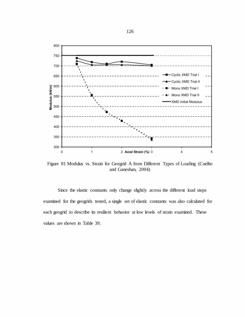
126
Figure 81 Modulus vs. Strain for Geogrid A from Different Types of Loading (Cuelho
and Ganeshan, 2004)
Since the elastic constants only change slightly across the different load steps
examined for the geogrids tested, a single set of elastic constants was also calculated for
each geogrid to describe its resilient behavior at low levels of strain examined. These
values are shown in Table 39.
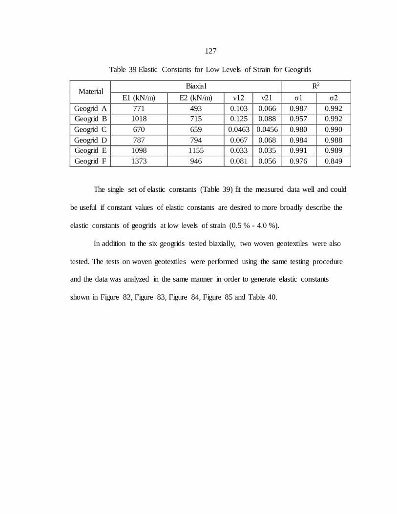
127
Table 39 Elastic Constants for Low Levels of Strain for Geogrids
Material Biaxial R2
E1 (kN/m) E2 (kN/m) ν12 ν21 σ1 σ2
Geogrid A 771 493 0.103 0.066 0.987 0.992
Geogrid B 1018 715 0.125 0.088 0.957 0.992
Geogrid C 670 659 0.0463 0.0456 0.980 0.990
Geogrid D 787 794 0.067 0.068 0.984 0.988
Geogrid E 1098 1155 0.033 0.035 0.991 0.989
Geogrid F 1373 946 0.081 0.056 0.976 0.849
The single set of elastic constants (Table 39) fit the measured data well and could
be useful if constant values of elastic constants are desired to more broadly describe the
elastic constants of geogrids at low levels of strain (0.5 % - 4.0 %).
In addition to the six geogrids tested biaxially, two woven geotextiles were also
tested. The tests on woven geotextiles were performed using the same testing procedure
and the data was analyzed in the same manner in order to generate elastic constants
shown in Figure 82, Figure 83, Figure 84, Figure 85 and Table 40.

128
Figure 82 Modulus of Elasticity, E1, vs. Load Step for All Geotextiles
Figure 83 Modulus of Elasticity, E2, vs. Load Step for All Geotextiles
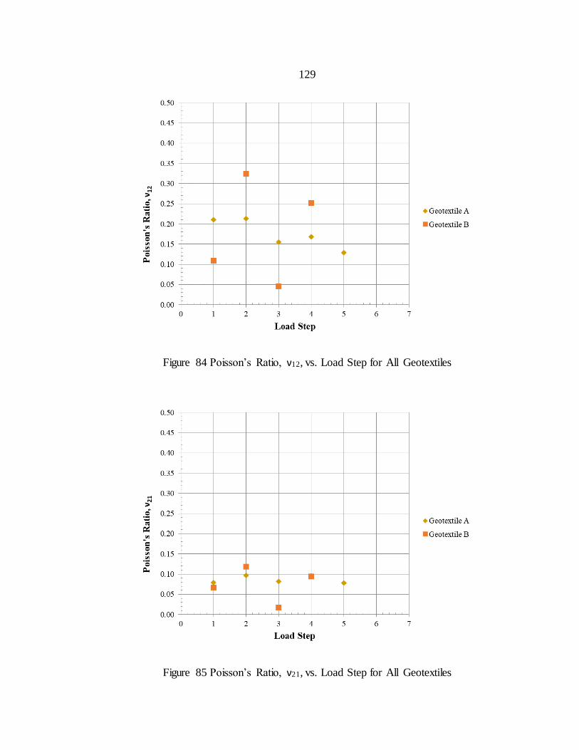
129
Figure 84 Poisson’s Ratio, ν12, vs. Load Step for All Geotextiles
Figure 85 Poisson’s Ratio, ν21, vs. Load Step for All Geotextiles
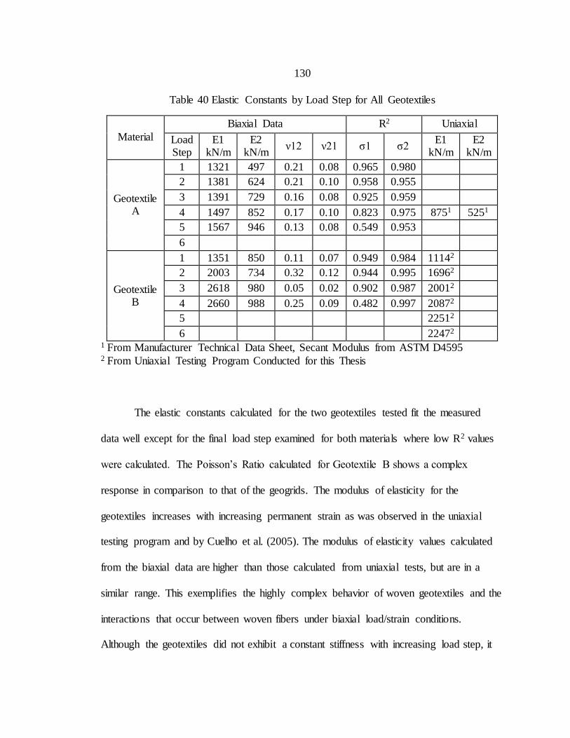
130
Table 40 Elastic Constants by Load Step for All Geotextiles
Material
Biaxial Data R2 Uniaxial
Load Step
E1 kN/m
E2 kN/m
ν12 ν21 σ1 σ2 E1
kN/m E2
kN/m
Geotextile A
1 1321 497 0.21 0.08 0.965 0.980
2 1381 624 0.21 0.10 0.958 0.955
3 1391 729 0.16 0.08 0.925 0.959
4 1497 852 0.17 0.10 0.823 0.975 8751 5251
5 1567 946 0.13 0.08 0.549 0.953
6
Geotextile B
1 1351 850 0.11 0.07 0.949 0.984 11142
2 2003 734 0.32 0.12 0.944 0.995 16962
3 2618 980 0.05 0.02 0.902 0.987 20012
4 2660 988 0.25 0.09 0.482 0.997 20872
5 22512
6 22472 1 From Manufacturer Technical Data Sheet, Secant Modulus from ASTM D4595 2 From Uniaxial Testing Program Conducted for this Thesis
The elastic constants calculated for the two geotextiles tested fit the measured
data well except for the final load step examined for both materials where low R2 values
were calculated. The Poisson’s Ratio calculated for Geotextile B shows a complex
response in comparison to that of the geogrids. The modulus of elasticity for the
geotextiles increases with increasing permanent strain as was observed in the uniaxial
testing program and by Cuelho et al. (2005). The modulus of elasticity values calculated
from the biaxial data are higher than those calculated from uniaxial tests, but are in a
similar range. This exemplifies the highly complex behavior of woven geotextiles and the
interactions that occur between woven fibers under biaxial load/strain conditions.
Although the geotextiles did not exhibit a constant stiffness with increasing load step, it
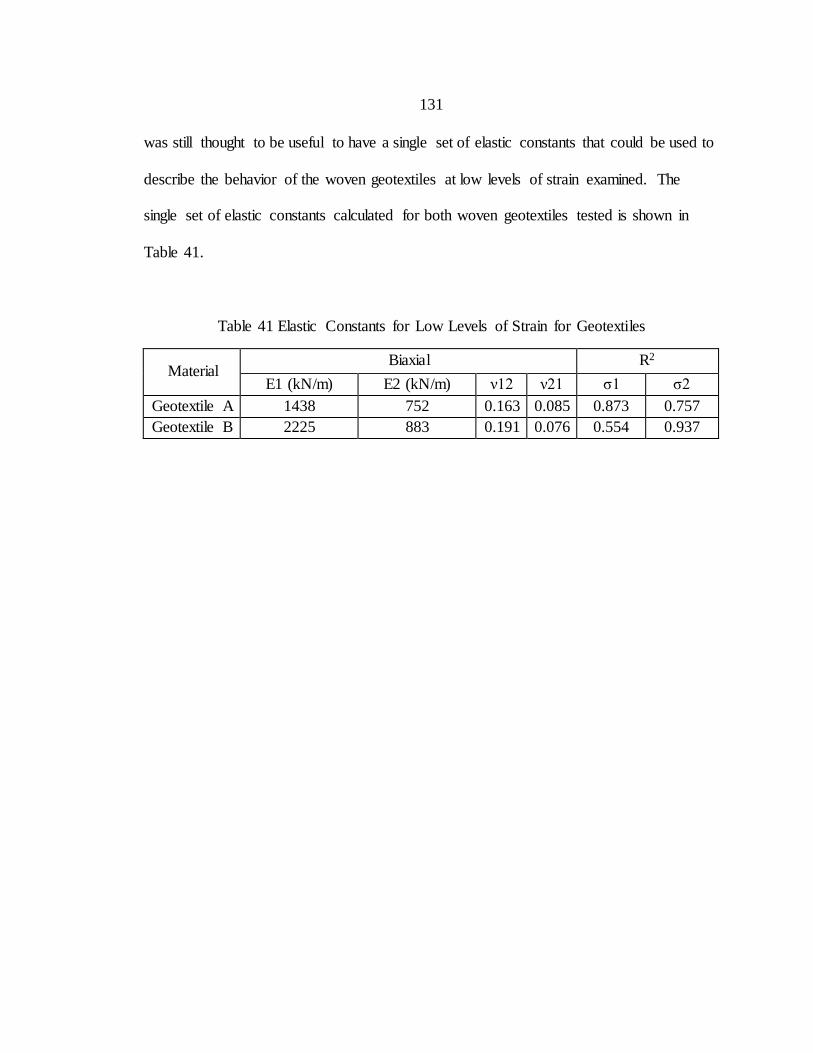
131
was still thought to be useful to have a single set of elastic constants that could be used to
describe the behavior of the woven geotextiles at low levels of strain examined. The
single set of elastic constants calculated for both woven geotextiles tested is shown in
Table 41.
Table 41 Elastic Constants for Low Levels of Strain for Geotextiles
Material Biaxial R2
E1 (kN/m) E2 (kN/m) ν12 ν21 σ1 σ2
Geotextile A 1438 752 0.163 0.085 0.873 0.757
Geotextile B 2225 883 0.191 0.076 0.554 0.937
132
CHAPTER SEVEN
SUMMARY AND RECOMMENDATIONS
Summary of Testing and Analysis
The uniaxial and biaxial testing programs implemented were successful in
characterizing the resilient response of different geosynthetic materials. The uniaxial
testing program was useful for creating a biaxial testing procedure on the experimental
biaxial testing device available. The uniaxial results were able to show that the four
different types of loading examined (cyclic stress relaxation, monotonic stress relaxation,
cyclic creep and monotonic creep) simulated an equivalent resilient response on a biaxial
geogrid and woven geotextile. The time to generate a representative resilient response in
the lab with these four types of loading was shown to be relatively quick (20 minutes).
The biaxial testing procedure was developed using available literature, the
uniaxial testing program results and considerations for the available biaxial testing
device. The procedure used was able to generate data that fit an orthotropic linear elastic
constitutive model that was used to calculate elastic constants for different geosynthetic
materials. The elastic constants were successfully solved for using a least squares
approximation for different geosynthetics. The elastic constants calculated using the least
squares approximation were reasonable values based upon how well they fit the measured
biaxial stress/strain data and their proximity to resilient uniaxial modulus values. The
elastic constants calculated from biaxial tests are not expected to be identical to uniaxial
values because the test conditions are different. Elastic constants calculated from biaxial
133
tests with an orthotropic linear elastic constitutive model provide a better representation
of geosynthetic material properties than uniaxial tests because Poisson’s ratio is included
in the model. Thus, the elastic constants calculated are more applicable for predicting the
stress/strain response of geosynthetics in field loading applications. The elastic constants
were calculated from stress/strain data after stress relaxation and creep so that they can be
used to describe a resilient response of geosynthetics expected in field loadings. The
elastic constants were calculated from stress/strain data from three modes of loading and
thus describe the response of geosynthetics in multiple field loading situations where
geosynthetics experience simultaneous loading in both directions, or plane strain loading.
Recommendations for Future Testing
The uniaxial tests performed were modeled after an existing ASTM standard
(D7556), and thus do not need significant modification or recommendations. The creep
tests however do not have an existing standard and could be investigated further to
confirm the conclusions drawn in this thesis. Due to time limitations, a robust uniaxial
creep testing program was not possible for this thesis and thus a small number of trials
were performed on only two materials. The creep properties of geosynthetics have been
studied in the past but not in the same format as was investigated for this research. To
examine the resilient response of geosynthetics after uniaxial creep, it is recommended
that a procedure modeled after ASTM D7556 be developed and implemented on more
materials with enough trials to determine if precision requirements in ASTM D7556 are
met.
134
Ideally more trials on all materials tested biaxially would have been performed to
try and quantify the precision of the data collected and what is possible with the given
biaxial device. More trials performed on the geotextiles could have helped better
understand the values of Poisson’s ratio reported at different load steps. More trials on
Geogrid E would also be helpful to confirm the very low Poisson’s ratio values calculated
for load step 1.
The biaxial tests on geosynthetics were modeled after the uniaxial testing
program, ASTM D7556 and biaxial tension tests performed on structural membranes.
The biaxial testing device used for this project was a relatively new testing device that
had not been used for any formal testing programs or robust research previously. This
created a lot of experimentation with the device in order to generate reasonably precise
data that was useful for determining the material response of geosynthetics. Some
improvements to the instrumentation and control of the device is necessary to generate
data with higher precision. The LVDTs used to measure strain in the materials are
accurate instruments, but attaching them to the geosynthetic at discrete points is not the
best way to measure strain in the material. The setup of the LVDTs inherently introduces
small amounts of human error that influence strain measurements between trials. It would
beneficial to use video software to observe the strain of all nodes in the interior portion of
the cruciform sample in order to generate a strain field. This type of approach would
eliminate human error and save time associated with testing setup. The measurement of
strain between discrete points also was problematic for the triaxial geogrid tested. The
triaxial geogrid was tested in all three modes of biaxial loading using the developed
135
testing procedure. The data generated from testing the triaxial geogrid was very erratic
and difficult to fit into the constitutive model. The data from the triaxial geogrid
ultimately was not used for calculation of elastic constants due to the quality of the data.
It was thought that the discrete measurement points of strain for the triaxial geogrid may
have caused some the data to be confusing and if a strain field was calculated then a
better representation of the material response could have been generated.
The mechanism through which the biaxial testing device created displacement in
the material could also be improved on future biaxial testing devices. The electric motor
was not ideal for loading materials because it is not technically creating a constant rate of
strain for the initial loading of a material after stress relaxation or creep. This is due to the
fact that the electric motor must accelerate to the desired speed before it operates at a
constant speed. The same is true when the motor is turned off as it must decelerate before
stopping. This deceleration causes difficulty in reaching the desired level of permanent
strain precisely in the testing procedure used. The permanent strain limits used for biaxial
tests were not precisely or consistently adhered to because of the human control of the
displacement and the deceleration of the motor. A major improvement necessary for
creating a more standardized testing procedure would be to setup the biaxial device so
that a testing procedure with precise permanent strain limits could be programmed. An
interface with feedback to the device control such as that on the uniaxial testing device
would be ideal so that the strain limits are precisely followed. The measurement of load
using load cells in the chains of the device was a smart way to design the biaxial testing
device but caused some minor problems. The weight of the load cells in the chains and
136
the self-weight of the chain cause a slight sagging in the chain at low levels of load. The
effect of this was not significant for this study because the data of interest was at loads
corresponding to 0.5 % strain and above where the sagging is minimal. In the future, it
may be desirable to measure load in all four directions if tests were performed on samples
at a 45 degree orientation to confirm that the load is equal on both sides of a sample.
Another improvement that could be made on the biaxial testing device is the
material gripping method. The material grips on the biaxial device did not cause any
issues with the data collected but could be improved. The rigid plates that were bolted
together to grip the material were very functional and cost-effective, but also required
significant time for testing setup. The geosynthetic also had to be modified to fit in the
grips for each testing sample and then manually centered in each grip. Eight bolts then
had to be tightened on all four grips, ensuring the material stayed centered the entire time.
This process was not difficult to perform but was much more time-intensive than using
the gripping method available for the uniaxial testing device. A possible improvement to
the biaxial testing device would be to have clamps more similar to those used in the
uniaxial testing device.
Overall, the biaxial device used for this thesis was an adequate device designed in
an intelligent and cost-effective manner for the testing of geosynthetics. However, the
device in conjunction with the procedure developed and number of trials performed on
each material was not able to produce the high quality, repeatable data that would be
necessary to create a standardized testing procedure such as ASTM D7556. Some
potential improvements could be made in the instrumentation for measuring strain and
137
controlling displacement. A photometric method for measuring strain would be
recommended so that a strain field is generated instead of measuring strain at discrete
points using LVDTs. A hydraulic loading mechanism that is controlled by a
programmable procedure would eliminate the need for a human controlled procedure and
a case by case analysis of data. This type of testing device would certainly be
significantly more expensive but might be necessary for creating a biaxial testing
procedure for simulating the resilient response of geosynthetics similar to the uniaxial
ASTM D7556 testing procedure.

138
REFERENCES CITED
139
ASCE/SEI 55-10. (2010). Standard for Tensile Membrane Structures
ASTM D7556. (2010). Standard Test Methods for Determining Small-Strain Tensile Properties of Geogrids and Geotextiles by In-Air Cyclic Tension Tests.
ASTM D4595. (2015). Standard Test Method for Determining Tensile Properties of Geogrids by the Single or Multi-Rib Tensile Method.
ASTM D4439. (2017a). Standard Terminology for Geosynthetics.
ASTM D4595. (2017b). Standard Test Method for Tensile Properties of Geotextiles by the Wide-Width Strip Method.
Beccarelli, P. (2015). The Development of Biaxial Testing Devices and Procedures for
Architectural Fabrics. In Biaxial Testing for Fabrics and Foils: Optimizing
Devices and Procedures (pp. 73-118). Cham: Springer International Publishing.
Bridgens, B., & Gosling, P. (2003). Biaxial fabric testing to determine in-situ material properties. Paper presented at the Proceedings of the Int. Conf. on Structural Membranes.
Bridgens, B., & Gosling, P. (2004). A new biaxial test protocol for architectural fabrics.
Paper presented at the IASS 2004 Symposium Montpellier: Shell and spatial structures from models to realisation.
Bridgens, B., & Gosling, P. (2010). Interpretation of results from the MSAJ “testing method for elastic constants of membrane materials”. Paper presented at the
Tensinet symposium. Chapra, S. C., & Canale, R. P. (1998). Numerical methods for engineers (Vol. 2):
McGraw-Hill New York.
Checkland, P., Bull, T., & Bakker, E. (1958). A two-dimensional load-extension tester for fabrics and film. Textile Research Journal, 28(5), 399-403.
Cuelho, E. (1998). Determination of Geosynthetic Constitutive Parameters and Soil/Geosynthetic Interaction by In-Air and In-Soil Experiments. (Master of
Science Master's), Montana State University, Bozeman, Montana. Cuelho, E., & Ganeshan, S. (2004). Developing Test Protocols to Determine
Geosynthetic Material Properties That Better Represent Traffic Loading Conditions. Western Transportation Institute, Montana State University–
Bozeman, USA.
140
Cuelho, E., Perkins, S., & Ganeshan, S. (2005). Determining geosynthetic material properties pertinent to reinforced pavement design. In Advances in Pavement
Engineering (pp. 1-12). Haas, R., & Dietzius, A. (1913). Stoffdehnung und Formänderung der Hülle von Prall-
Luftschiffen: Springer.
Hangen, Detert, & Alexiew. (2008). BIAXIAL TESTING OF GEOGRIDS: RECENT DEVELOPMENTS. EUROGEO, 4.
Klein, W. G. (1959). Stress-Strain Response of Fabrics Under Two-Dimensional Loading: Part I: The RL Biaxial Tester. Textile Research Journal, 29(10), 816-
821. Koerner, R. M. (2012). Designing with Geosynthetics - 6Th Edition: Xlibris US.
Krause, D. L., & Bartolotta, P. A. (2001). Biaxial Testing of High-Strength Fabric
Improves Design of Inflatable Radar Domes. Kupec, J., & McGown, A. (2004). The Biaxial load-strain behaviour of Biaxial Geogrids.
Geoasia04.
McGown, A., Kupec, J., Heerten, G., & Voskamp, W. (2004). Current Approaches to the Determination of the Design Stiffness and Strength of Polymeric Biaxial Geogrids. Vorträge der Baugrundtagung, 123-130.
MSAJ. (1995). Testing Method for Elastic Constants of Membrane Materials. In (Vol.
(MSAJ/M-02-1995), pp. 28). Toranomon, Minatoku, Toyko, Japan: The Membrane Structures Association of Japan.
Perkins, S. (2000). Constitutive modeling of geosynthetics. Geotextiles and Geomembranes, 18(5), 273-292.
Reichardt, C., Woo, H., & Montgomery, D. (1953). A two-dimensional load-extension
tester for woven fabrics. Textile Research Journal, 23(6), 424-428.
Valero, S. N., Sprague, C. J., & Wrigley, N. E. (2014). Full Scale Trafficking of Geogrid
Reinforced Sections Under Realisitic Service Conditions. Paper presented at the International Conference on Geosynthetics, Berlin, Germany.
Van Craenenbroeck, M., Puystiens, S., De Laet, L., Van Hemelrijck, D., & Mollaert, M. (2015). Biaxial testing of fabric materials and deriving their material properties–
A quantitative study. Paper presented at the Proceedings of the International Association for Shell and Spatial structures (IASS) symposium.

141
APPENDICES
142
APPENDIX A
NONLINEAR LEAST SQUARES APPROXIMATION FOR SOLVING ELASTIC
CONSTANTS
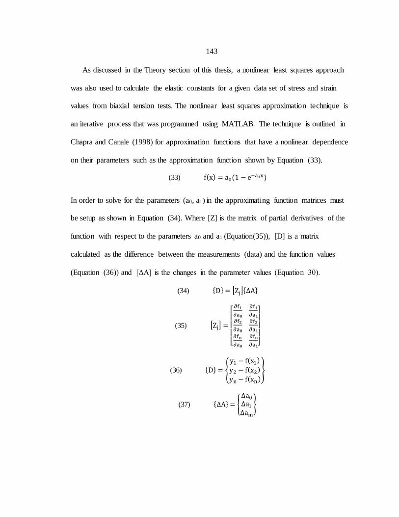
143
As discussed in the Theory section of this thesis, a nonlinear least squares approach
was also used to calculate the elastic constants for a given data set of stress and strain
values from biaxial tension tests. The nonlinear least squares approximation technique is
an iterative process that was programmed using MATLAB. The technique is outlined in
Chapra and Canale (1998) for approximation functions that have a nonlinear dependence
on their parameters such as the approximation function shown by Equation (33).
(33) f(x) = a0(1 − e−a1x)
In order to solve for the parameters (a0, a1) in the approximating function matrices must
be setup as shown in Equation (34). Where [Z] is the matrix of partial derivatives of the
function with respect to the parameters a0 and a1 (Equation(35)), [D] is a matrix
calculated as the difference between the measurements (data) and the function values
(Equation (36)) and [ΔA] is the changes in the parameter values (Equation 30).
(34) {D} = [Zj]{ΔA}
(35) [Zj] =
[ ∂f1
∂a0
∂f1
∂a1∂f2
∂a0
∂f2
∂a1
∂fn
∂a0
∂fn
∂a1]
(36) {D} = {
y1 − f(x1)
y2 − f(x2)
yn − f(xn)}
(37) {ΔA} = {Δa0
Δa1Δam
}
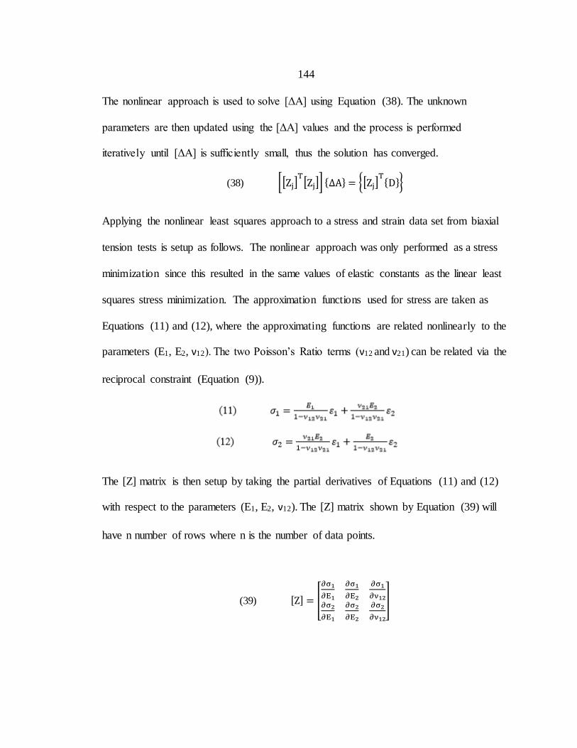
144
The nonlinear approach is used to solve [ΔA] using Equation (38). The unknown
parameters are then updated using the [ΔA] values and the process is performed
iteratively until [ΔA] is sufficiently small, thus the solution has converged.
(38) [[Zj]T[Zj]] {ΔA} = {[Zj]
T{D}}
Applying the nonlinear least squares approach to a stress and strain data set from biaxial
tension tests is setup as follows. The nonlinear approach was only performed as a stress
minimization since this resulted in the same values of elastic constants as the linear least
squares stress minimization. The approximation functions used for stress are taken as
Equations (11) and (12), where the approximating functions are related nonlinearly to the
parameters (E1, E2, ν12). The two Poisson’s Ratio terms (ν12 and ν21) can be related via the
reciprocal constraint (Equation (9)).
The [Z] matrix is then setup by taking the partial derivatives of Equations (11) and (12)
with respect to the parameters (E1, E2, ν12). The [Z] matrix shown by Equation (39) will
have n number of rows where n is the number of data points.
(39) [Z] = [
∂σ1
∂E1
∂σ1
∂E2
∂σ1
∂ν12∂σ2
∂E1
∂σ2
∂E2
∂σ2
∂ν12
]
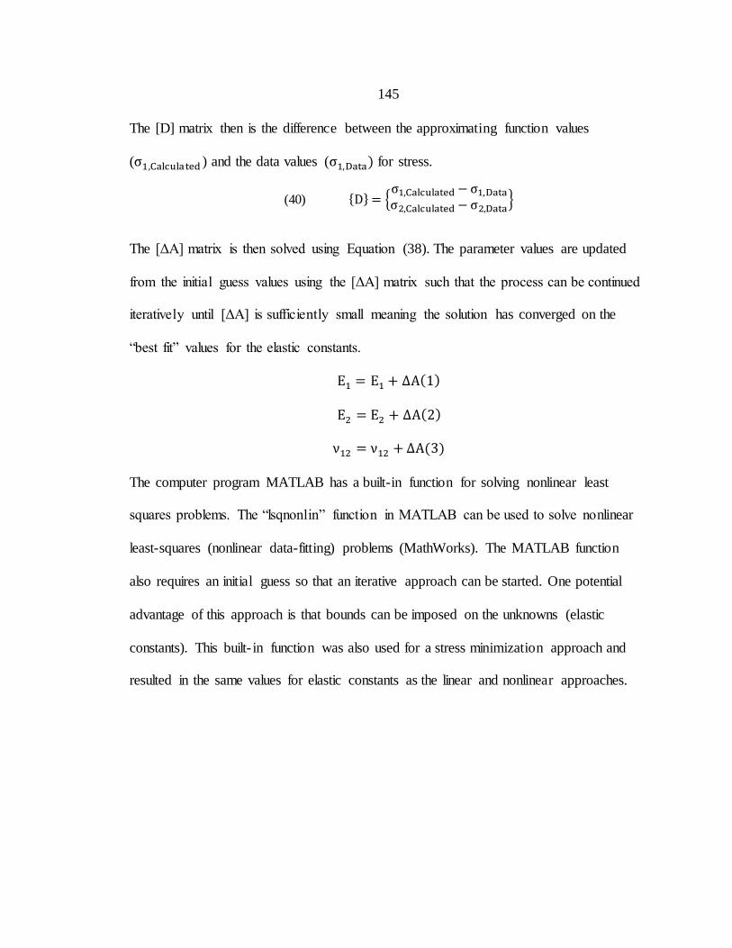
145
The [D] matrix then is the difference between the approximating function values
(σ1,Calculated ) and the data values (σ1,Data) for stress.
(40) {D} = {σ1,Calculated − σ1,Data
σ2,Calculated − σ2,Data}
The [ΔA] matrix is then solved using Equation (38). The parameter values are updated
from the initial guess values using the [ΔA] matrix such that the process can be continued
iteratively until [ΔA] is sufficiently small meaning the solution has converged on the
“best fit” values for the elastic constants.
E1 = E1 + ΔA(1)
E2 = E2 + ΔA(2)
ν12 = ν12 + ΔA(3)
The computer program MATLAB has a built-in function for solving nonlinear least
squares problems. The “lsqnonlin” function in MATLAB can be used to solve nonlinear
least-squares (nonlinear data-fitting) problems (MathWorks). The MATLAB function
also requires an initial guess so that an iterative approach can be started. One potential
advantage of this approach is that bounds can be imposed on the unknowns (elastic
constants). This built- in function was also used for a stress minimization approach and
resulted in the same values for elastic constants as the linear and nonlinear approaches.

146
APPENDIX B
LOAD PER UNIT WIDTH VS. STRAIN PLOTS FOR BIAXIAL TESTS
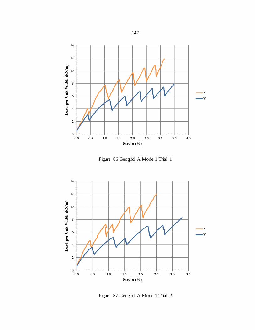
147
Figure 86 Geogrid A Mode 1 Trial 1
Figure 87 Geogrid A Mode 1 Trial 2
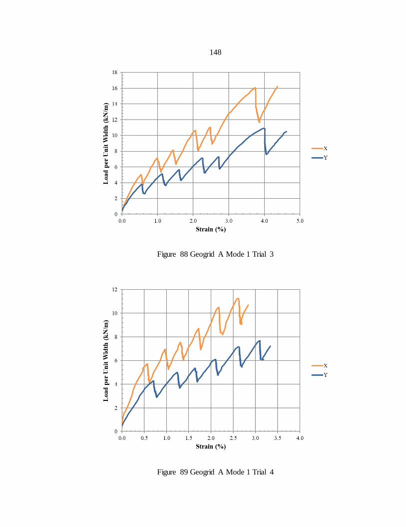
148
Figure 88 Geogrid A Mode 1 Trial 3
Figure 89 Geogrid A Mode 1 Trial 4
149
Figure 90 Geogrid A Mode 1 Trial 5
Figure 91 Geogrid A Mode 1 Trial 6
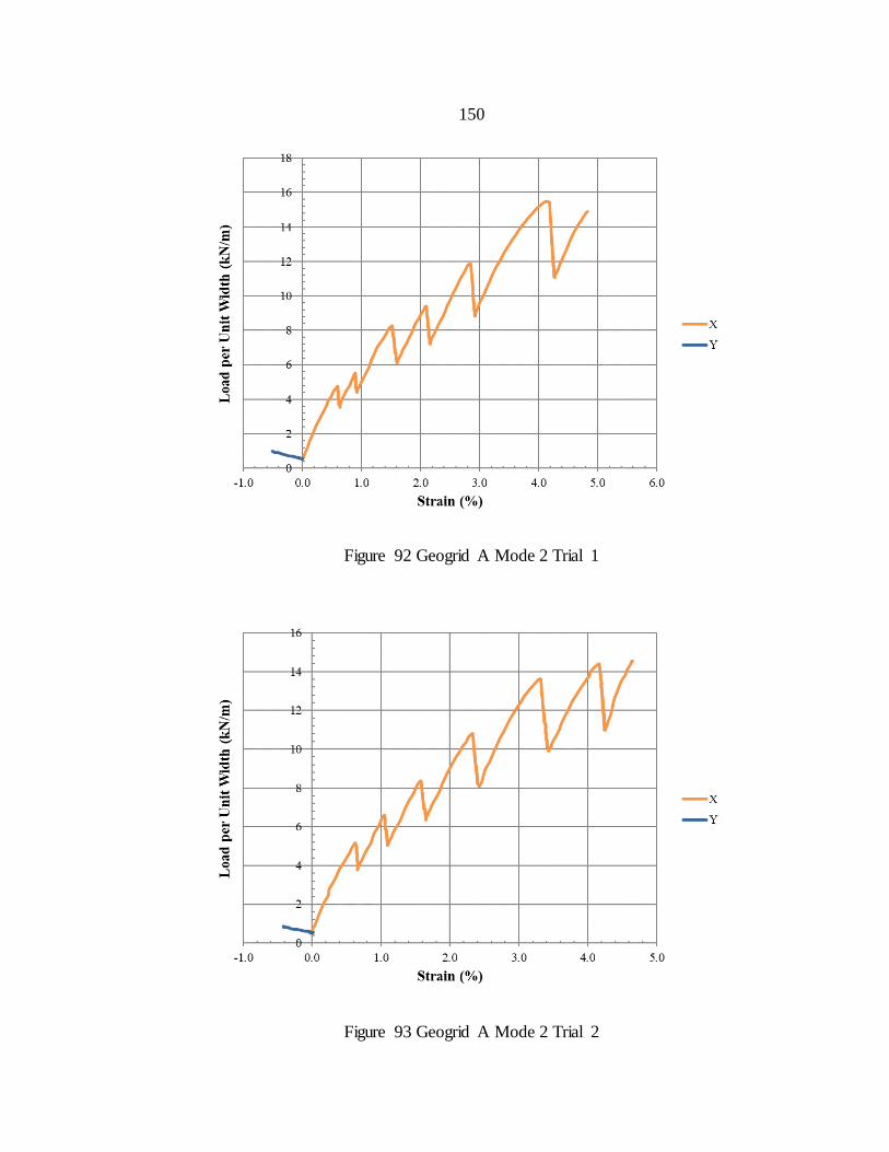
150
Figure 92 Geogrid A Mode 2 Trial 1
Figure 93 Geogrid A Mode 2 Trial 2
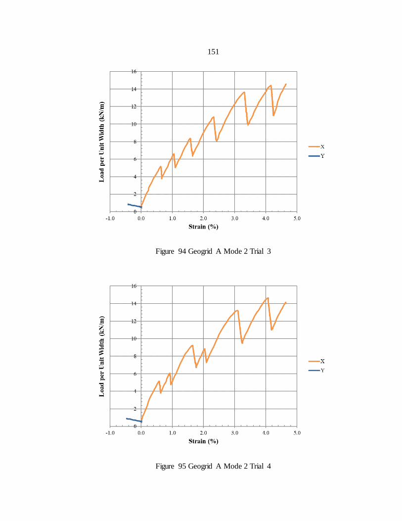
151
Figure 94 Geogrid A Mode 2 Trial 3
Figure 95 Geogrid A Mode 2 Trial 4
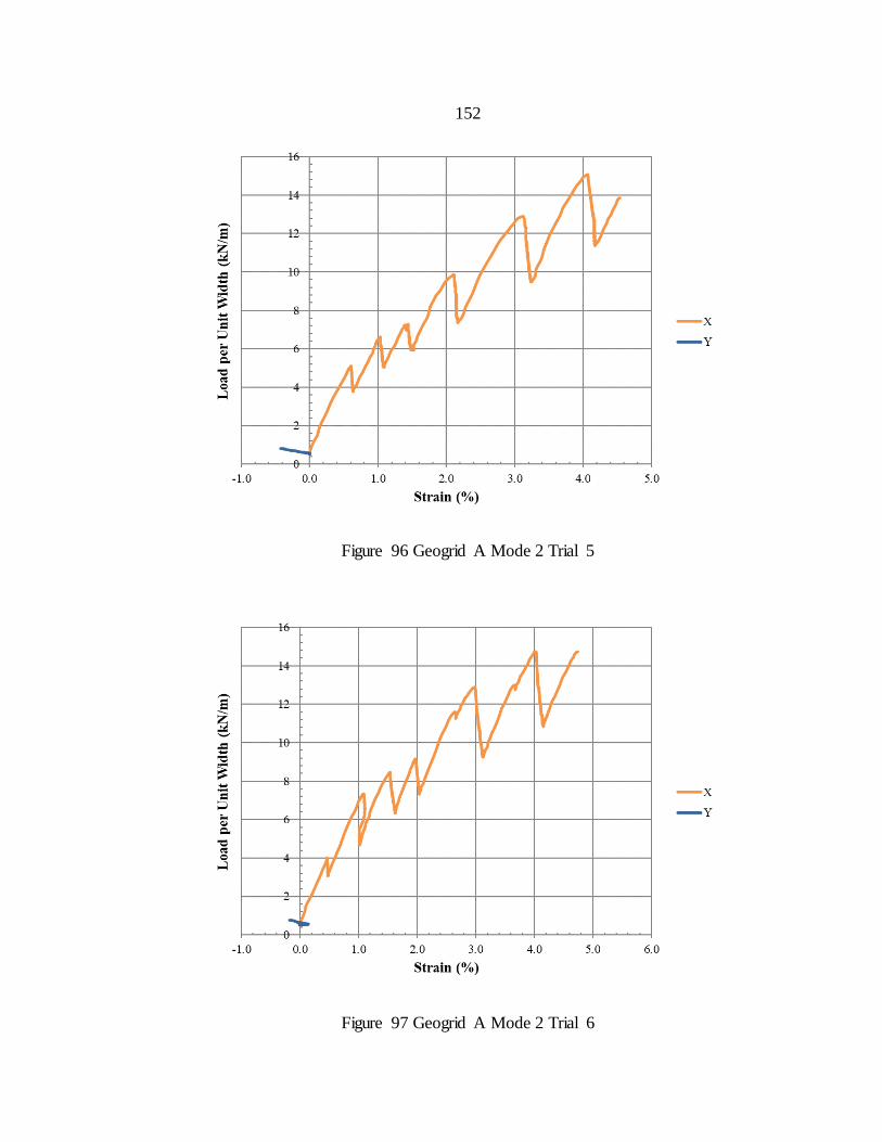
152
Figure 96 Geogrid A Mode 2 Trial 5
Figure 97 Geogrid A Mode 2 Trial 6

153
The irregularities seen on these load per unit width vs. strain plots between 2.0 %
and 3.0 % strain and 3.0 % and 4.0 % strain are due to the motor stopping automatically
then manually being restarted it at lower motor speeds to try to reach the next permanent
strain limit. This process had to be repeated multiple times for other materials and is why
the curve may appear irregular. This was acceptable because the only data of interest is
the initial loading after stress relaxation/creep.
Figure 98 Geogrid A Mode 3 Trial 1
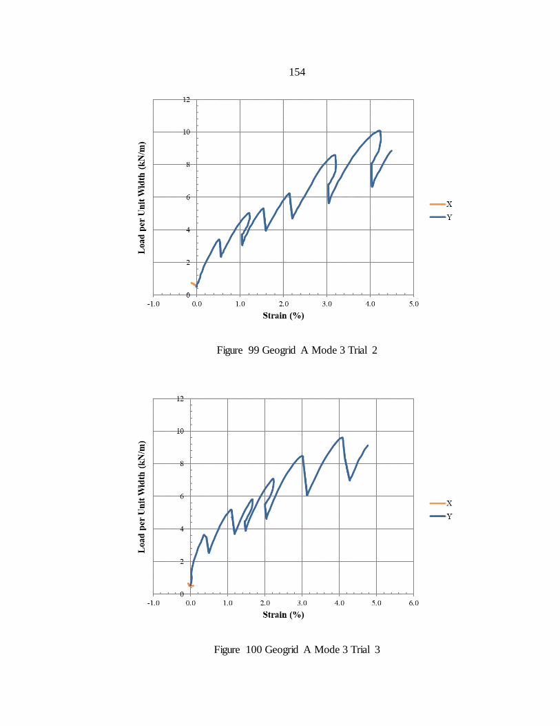
154
Figure 99 Geogrid A Mode 3 Trial 2
Figure 100 Geogrid A Mode 3 Trial 3
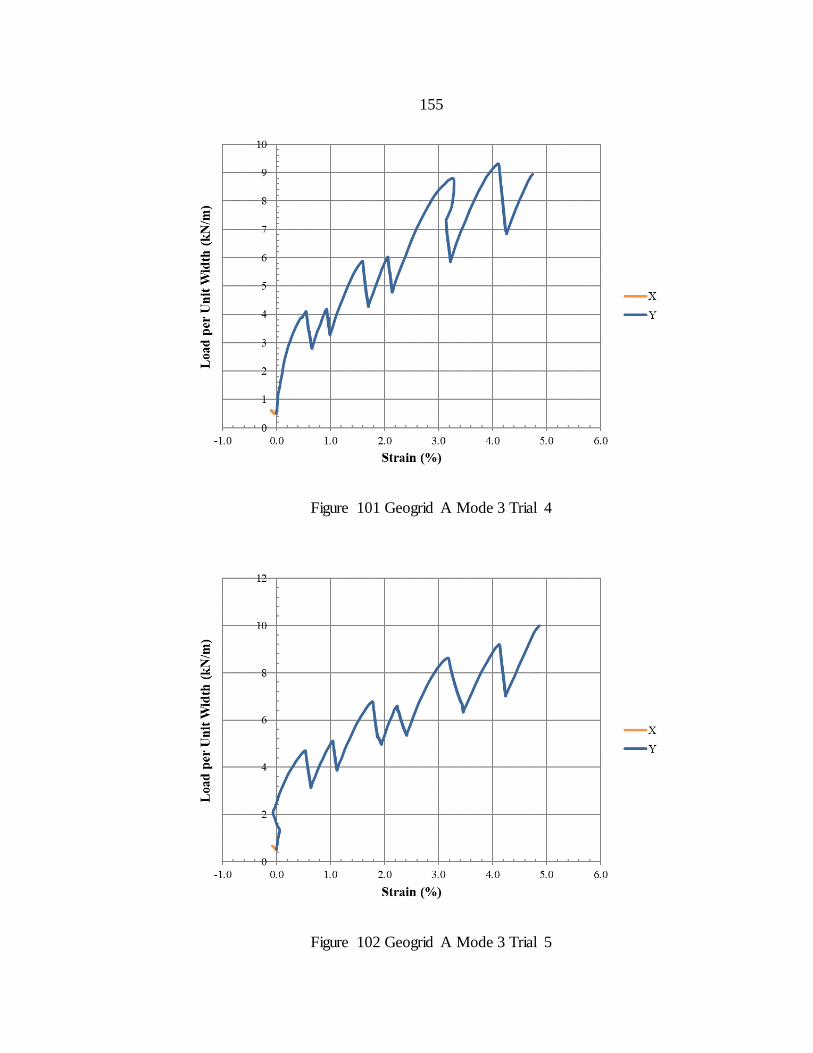
155
Figure 101 Geogrid A Mode 3 Trial 4
Figure 102 Geogrid A Mode 3 Trial 5
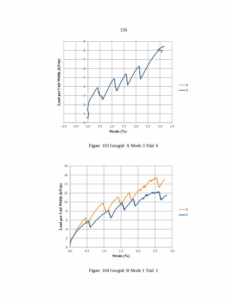
156
Figure 103 Geogrid A Mode 3 Trial 6
Figure 104 Geogrid B Mode 1 Trial 2
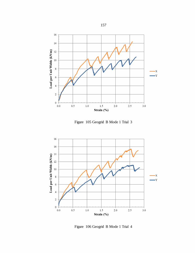
157
Figure 105 Geogrid B Mode 1 Trial 3
Figure 106 Geogrid B Mode 1 Trial 4
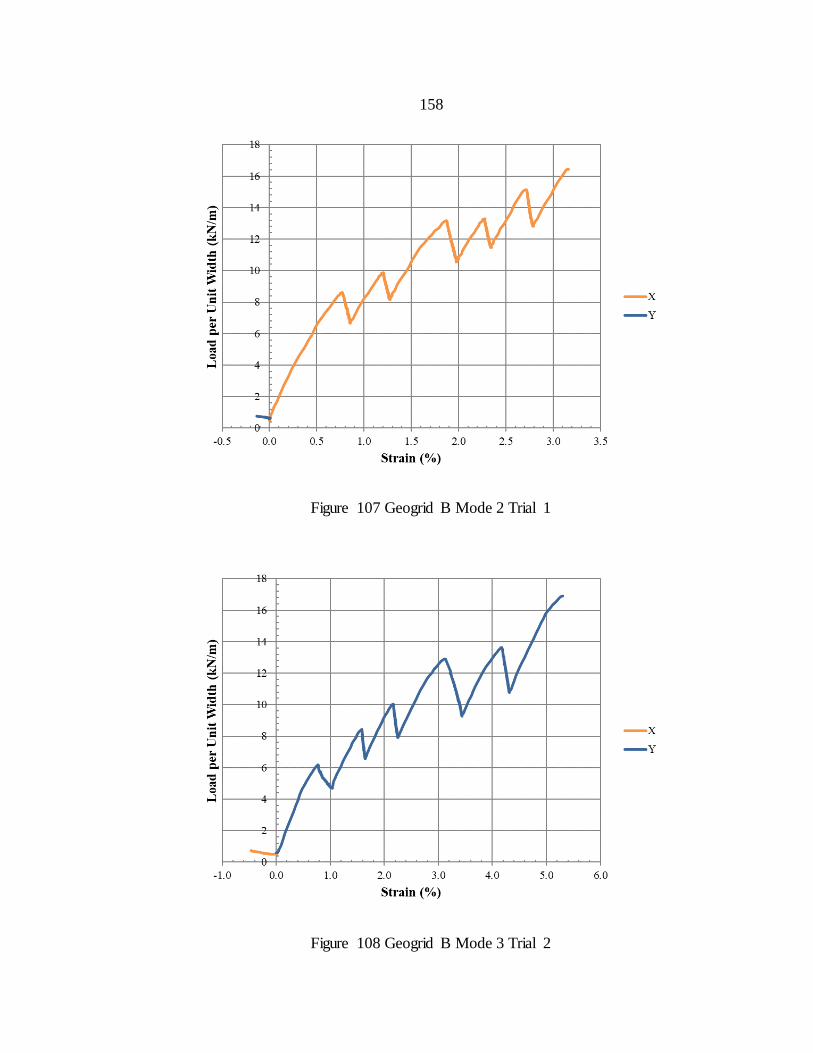
158
Figure 107 Geogrid B Mode 2 Trial 1
Figure 108 Geogrid B Mode 3 Trial 2
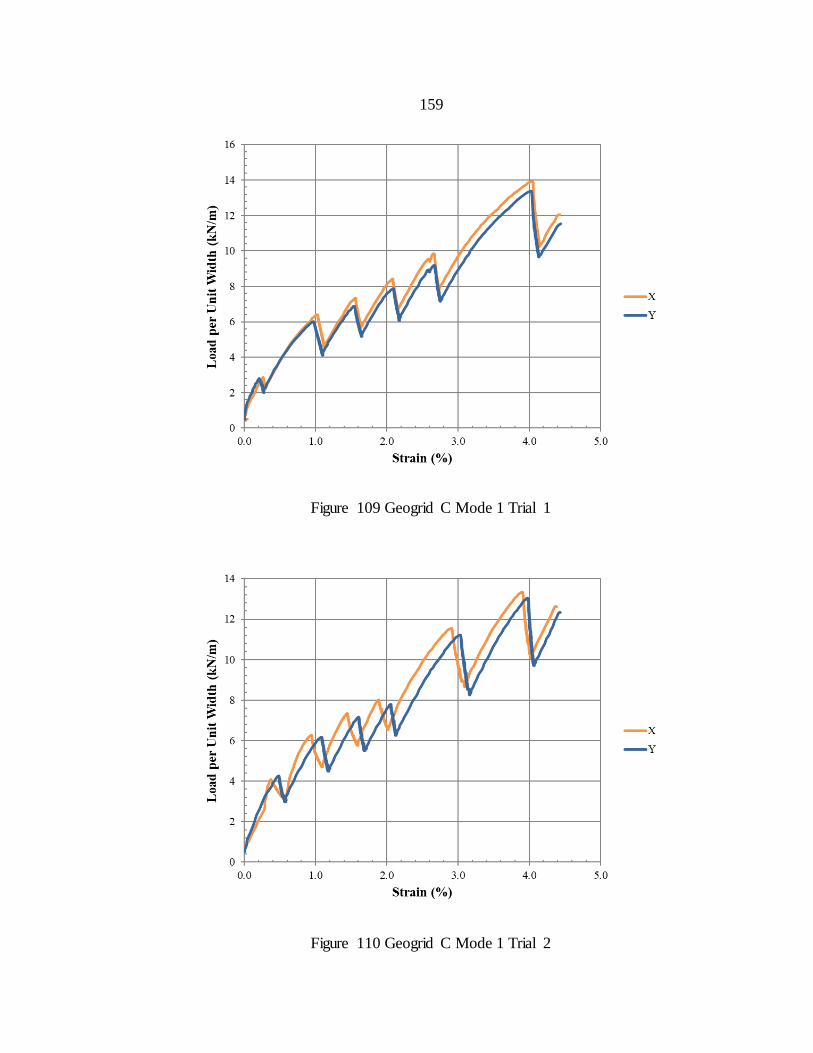
159
Figure 109 Geogrid C Mode 1 Trial 1
Figure 110 Geogrid C Mode 1 Trial 2
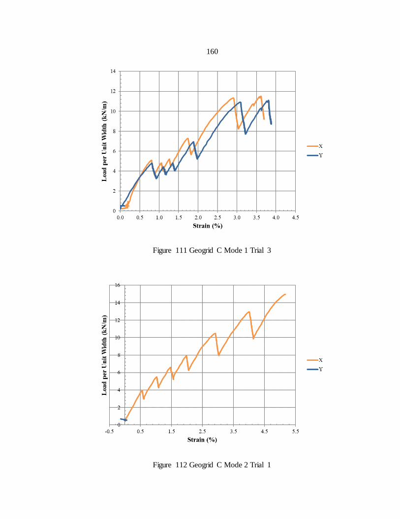
160
Figure 111 Geogrid C Mode 1 Trial 3
Figure 112 Geogrid C Mode 2 Trial 1
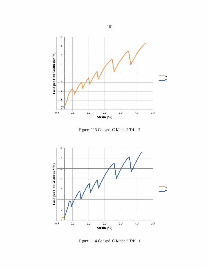
161
Figure 113 Geogrid C Mode 2 Trial 2
Figure 114 Geogrid C Mode 3 Trial 1
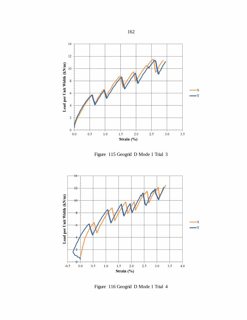
162
Figure 115 Geogrid D Mode 1 Trial 3
Figure 116 Geogrid D Mode 1 Trial 4
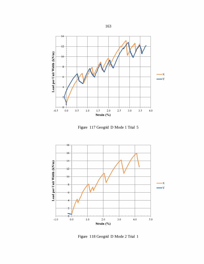
163
Figure 117 Geogrid D Mode 1 Trial 5
Figure 118 Geogrid D Mode 2 Trial 1
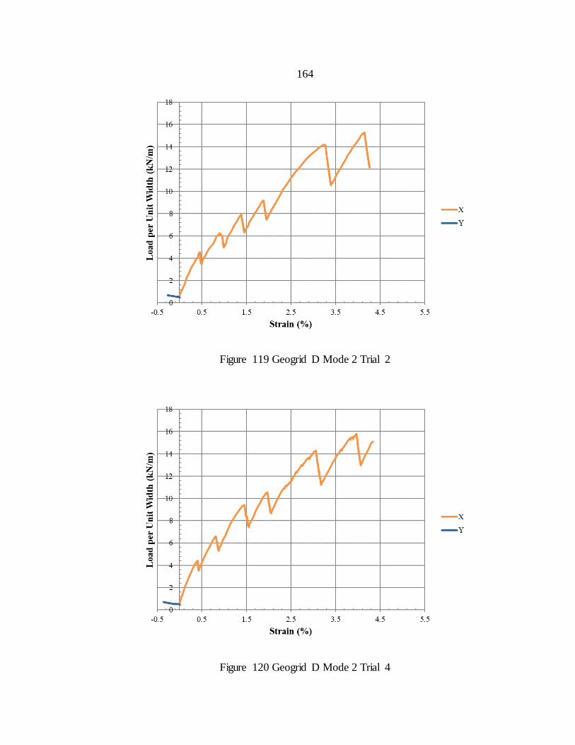
164
Figure 119 Geogrid D Mode 2 Trial 2
Figure 120 Geogrid D Mode 2 Trial 4
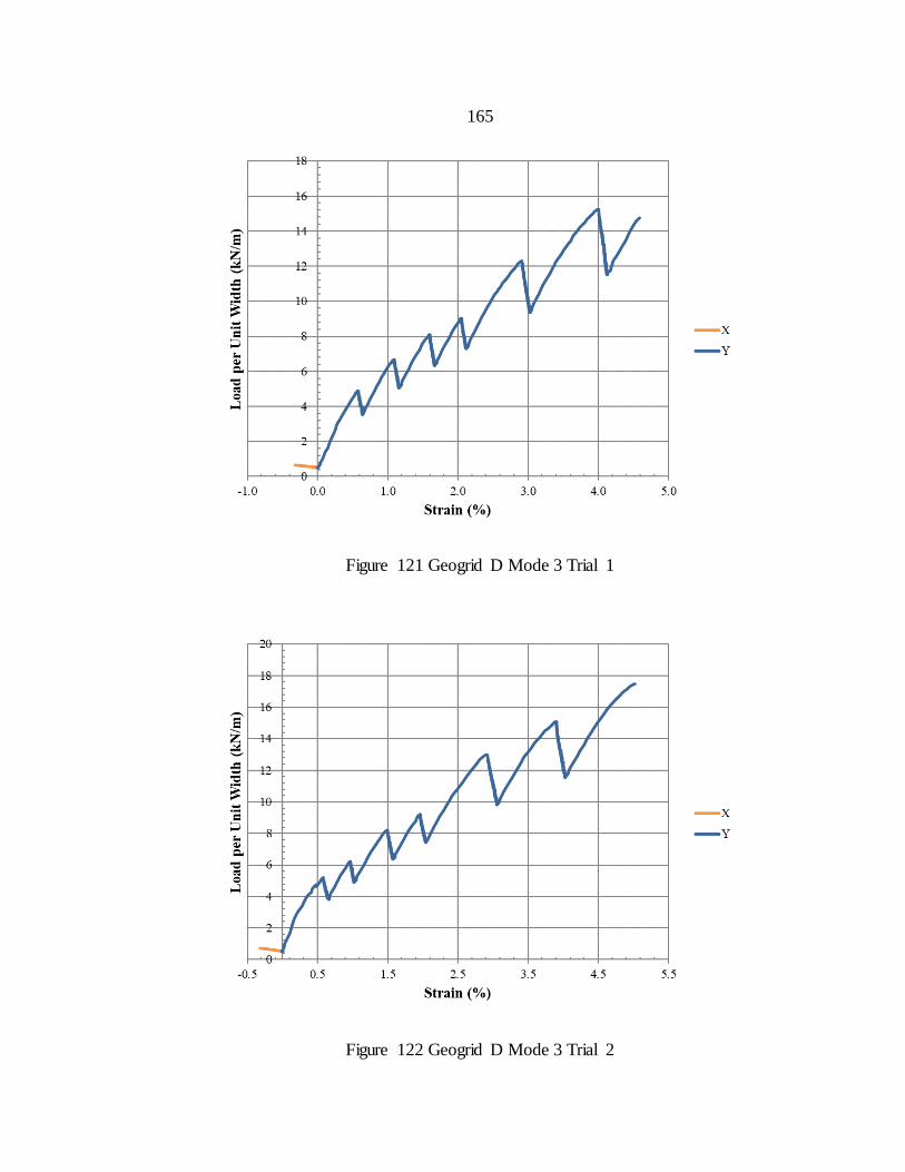
165
Figure 121 Geogrid D Mode 3 Trial 1
Figure 122 Geogrid D Mode 3 Trial 2
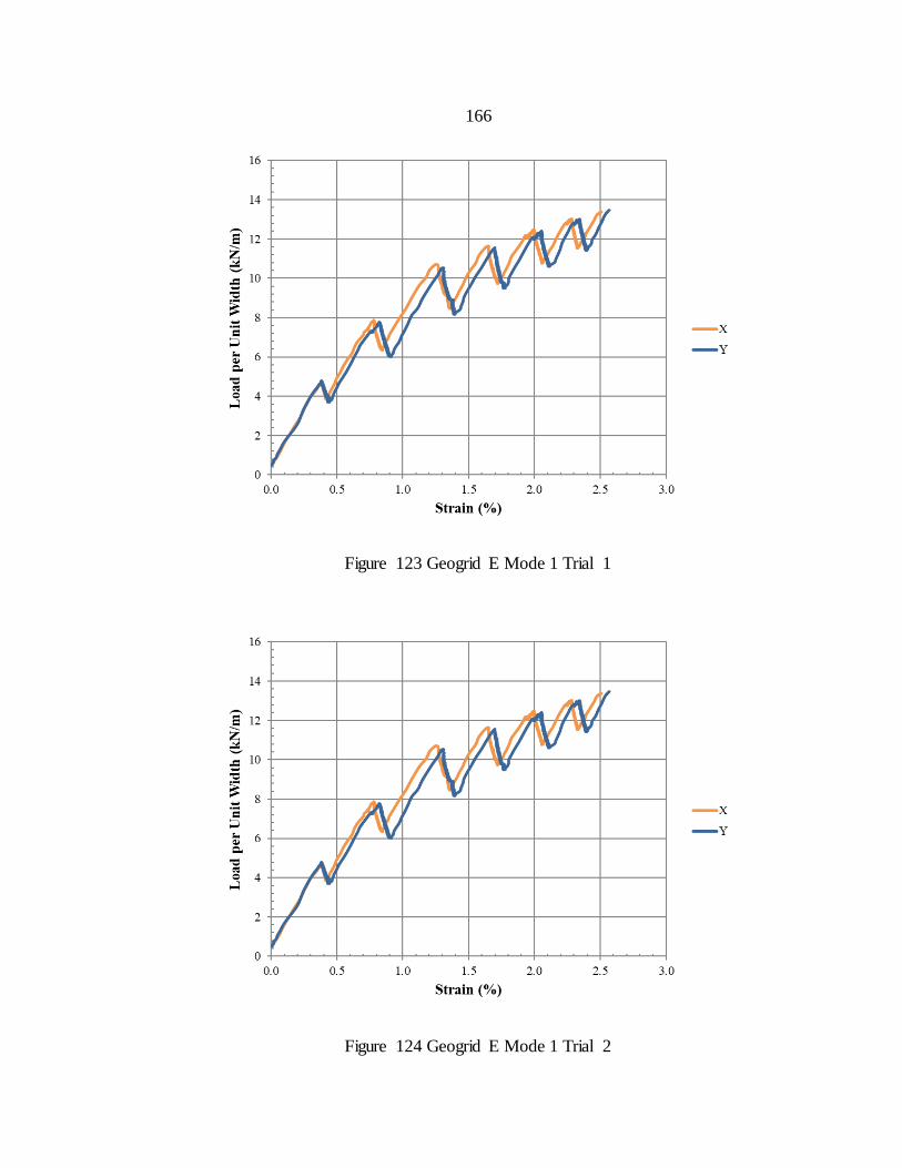
166
Figure 123 Geogrid E Mode 1 Trial 1
Figure 124 Geogrid E Mode 1 Trial 2
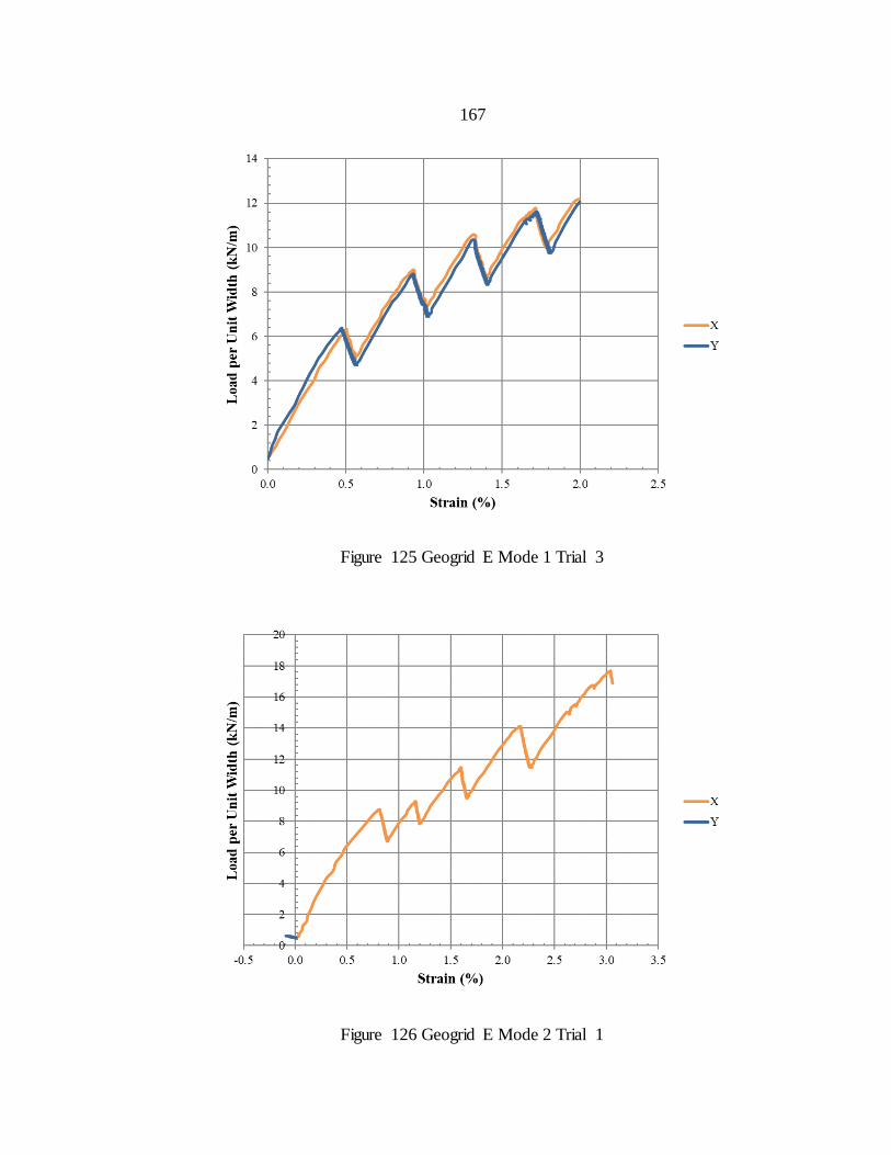
167
Figure 125 Geogrid E Mode 1 Trial 3
Figure 126 Geogrid E Mode 2 Trial 1
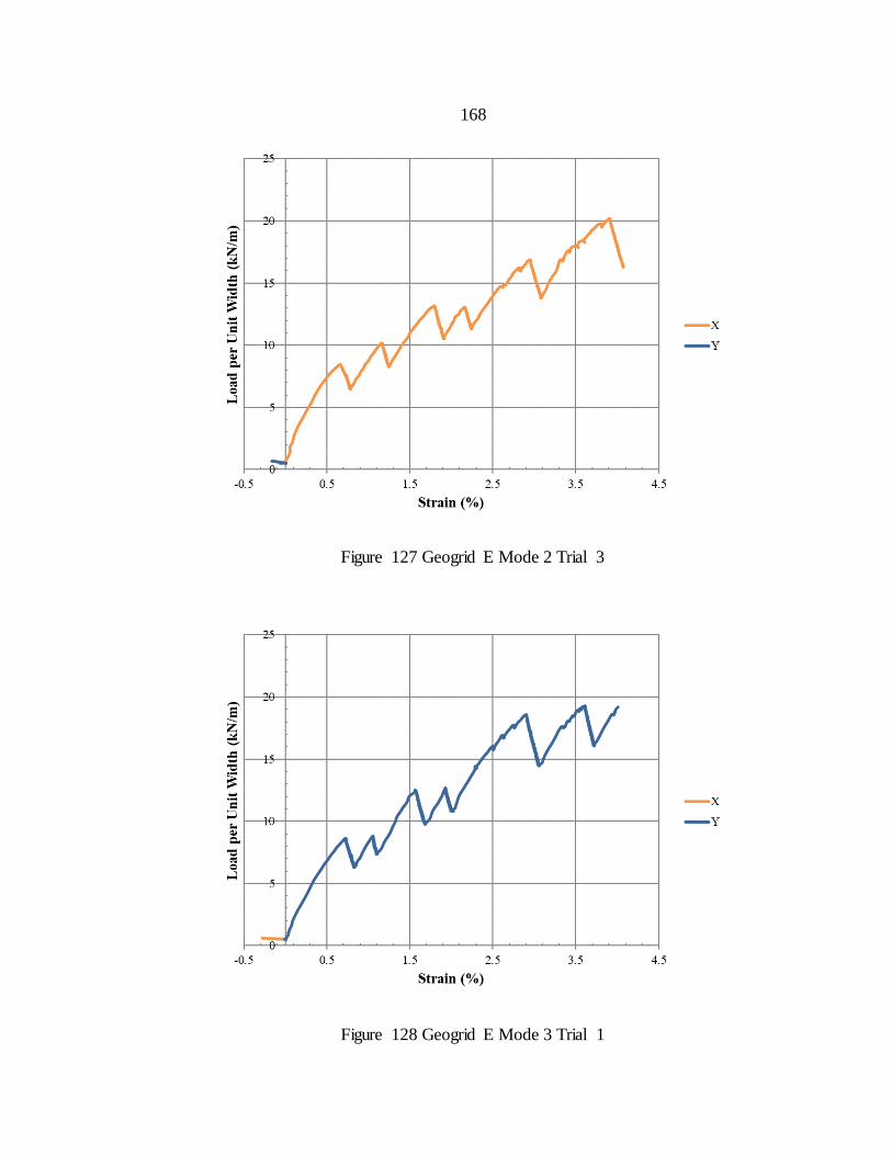
168
Figure 127 Geogrid E Mode 2 Trial 3
Figure 128 Geogrid E Mode 3 Trial 1
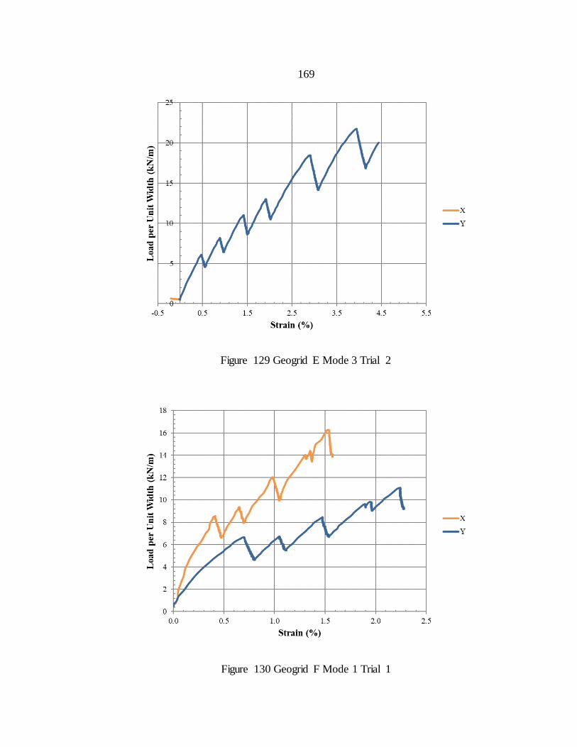
169
Figure 129 Geogrid E Mode 3 Trial 2
Figure 130 Geogrid F Mode 1 Trial 1
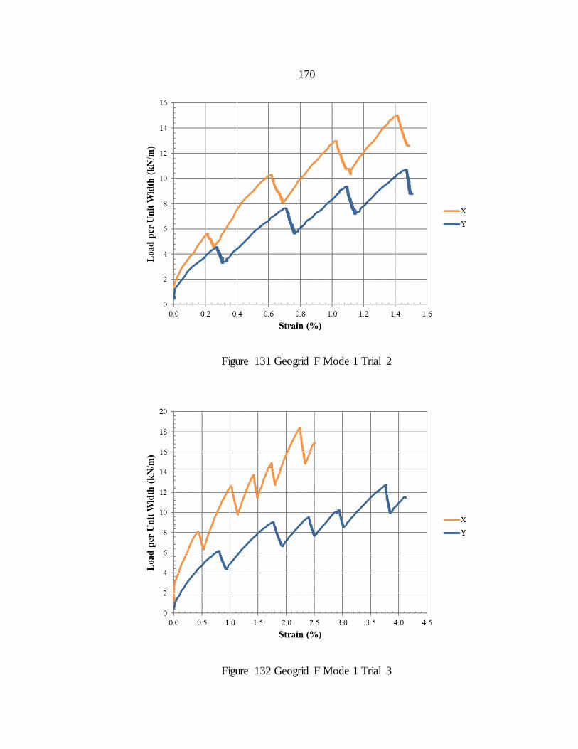
170
Figure 131 Geogrid F Mode 1 Trial 2
Figure 132 Geogrid F Mode 1 Trial 3
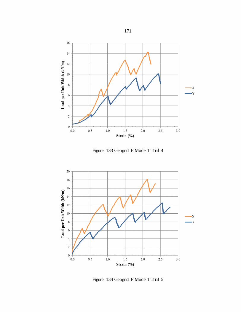
171
Figure 133 Geogrid F Mode 1 Trial 4
Figure 134 Geogrid F Mode 1 Trial 5
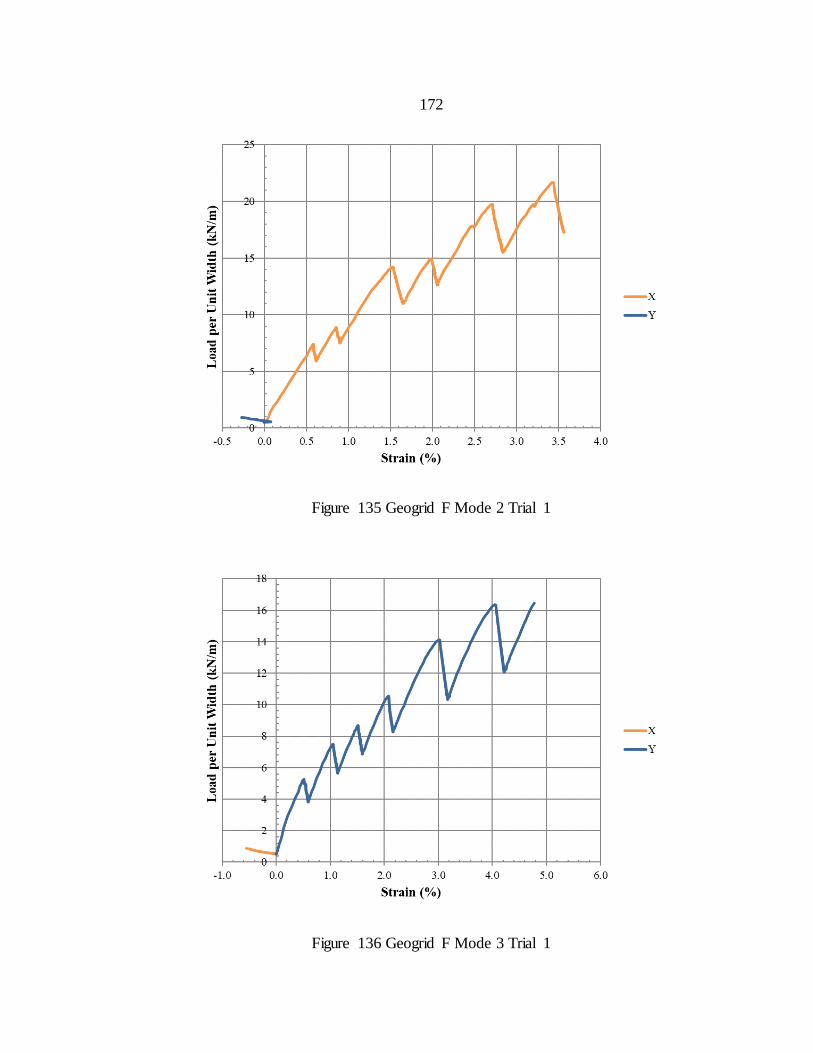
172
Figure 135 Geogrid F Mode 2 Trial 1
Figure 136 Geogrid F Mode 3 Trial 1
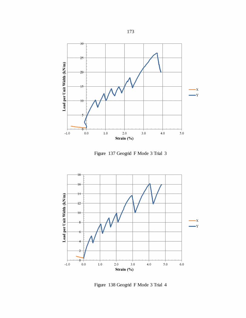
173
Figure 137 Geogrid F Mode 3 Trial 3
Figure 138 Geogrid F Mode 3 Trial 4
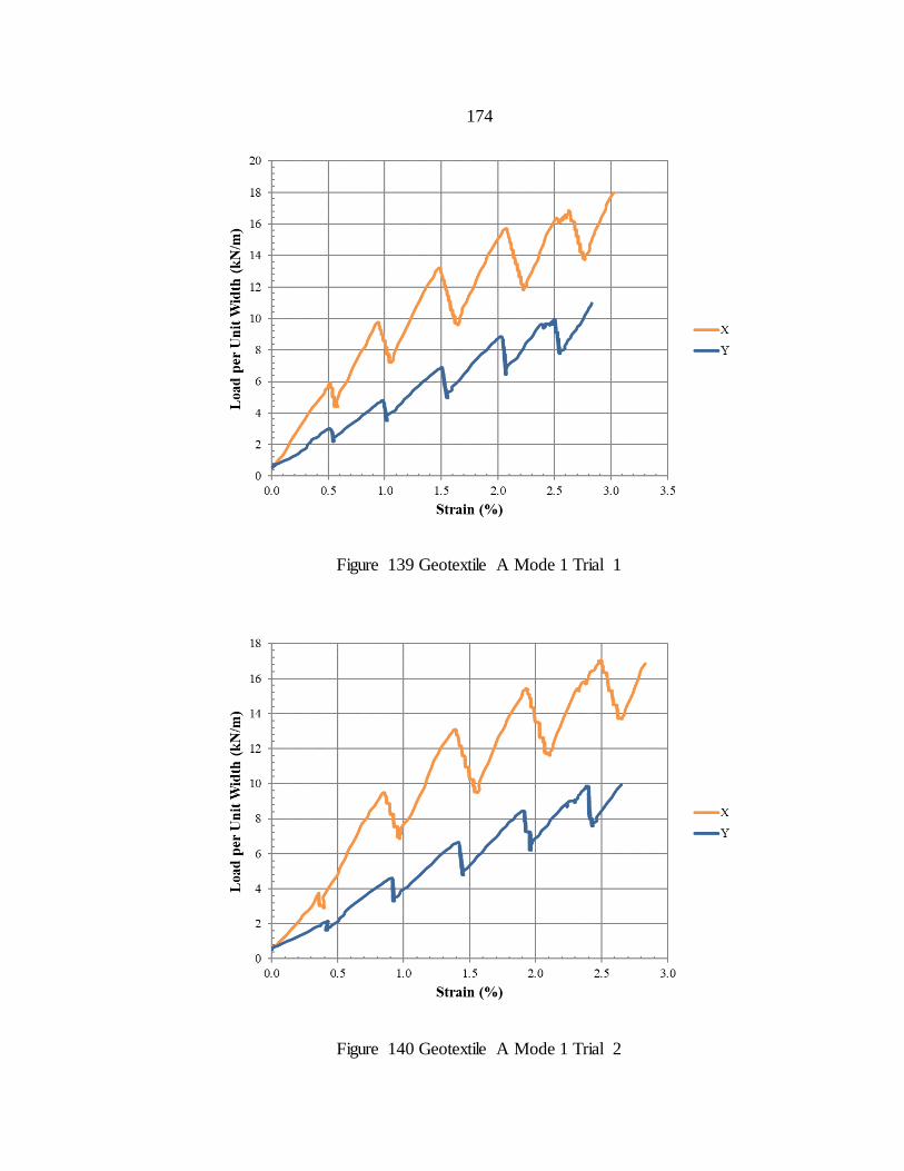
174
Figure 139 Geotextile A Mode 1 Trial 1
Figure 140 Geotextile A Mode 1 Trial 2
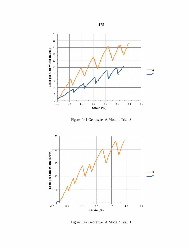
175
Figure 141 Geotextile A Mode 1 Trial 3
Figure 142 Geotextile A Mode 2 Trial 1
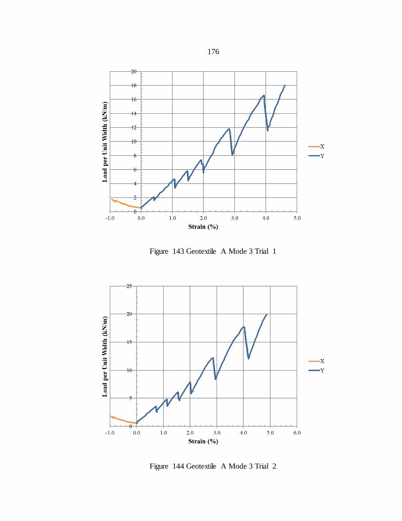
176
Figure 143 Geotextile A Mode 3 Trial 1
Figure 144 Geotextile A Mode 3 Trial 2
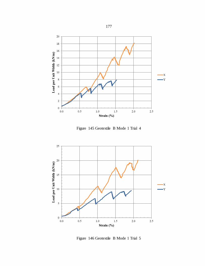
177
Figure 145 Geotextile B Mode 1 Trial 4
Figure 146 Geotextile B Mode 1 Trial 5
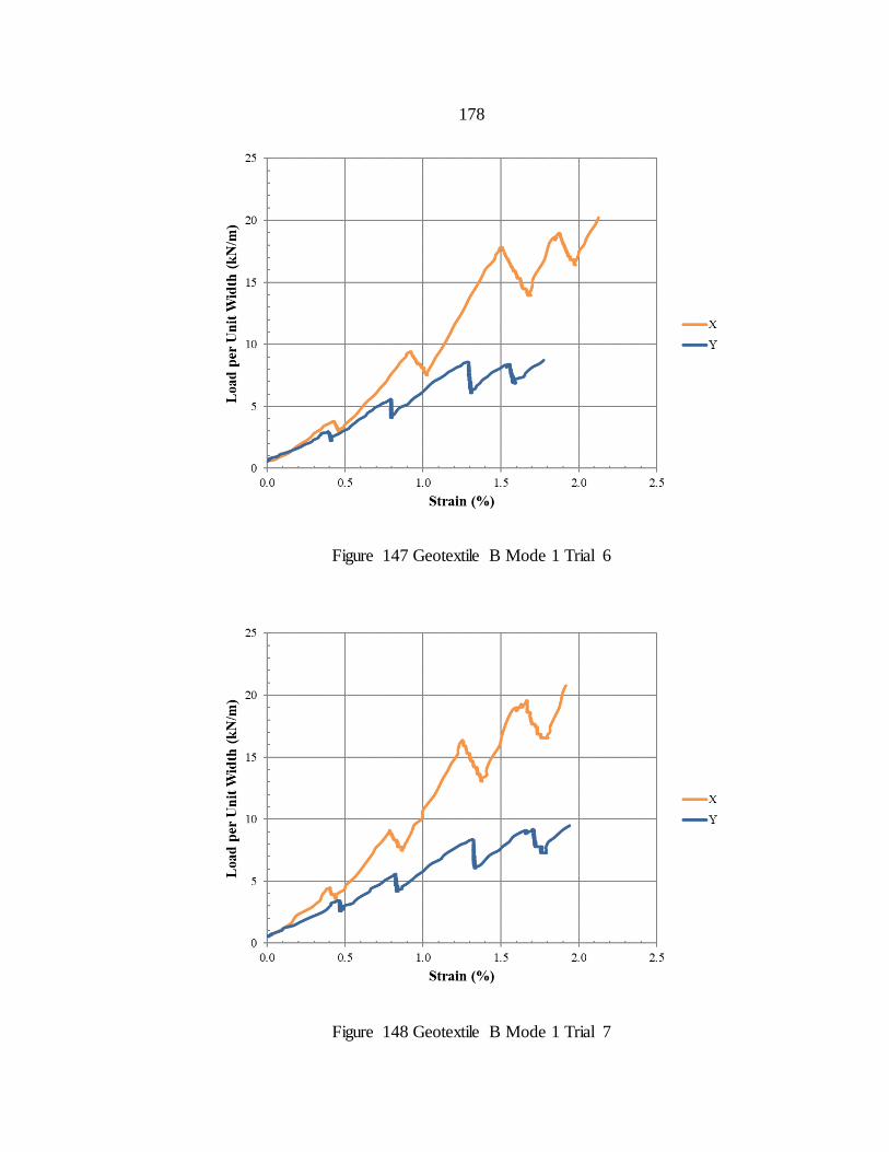
178
Figure 147 Geotextile B Mode 1 Trial 6
Figure 148 Geotextile B Mode 1 Trial 7
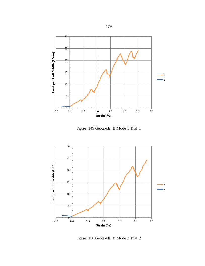
179
Figure 149 Geotextile B Mode 1 Trial 1
Figure 150 Geotextile B Mode 2 Trial 2

180
Figure 151 Geotextile B Mode 3 Trial 1

181
APPENDIX C
DRAFT OF TESTING STANDARD FOR DETERMINATION OF ELASTIC
CONSTANTS FOR GEOSYNTHETICS USING IN-AIR BIAXIAL TENSION TESTS

182
Scope
This test method covers the determination of the elastic constants of geogrids and geotextiles subjected to small-strain biaxial tension tests meant to represent loads
experienced by geosynthetics in field loadings such as reinforced pavement.
Terminology
Aperture – Openings in a geogrid, space between by ribs and nodes. Cross-machine direction (XMD) - Direction of geosynthetic along the width of the roll,
perpendicular to machine direction. Cruciform sample – Shape of biaxial specimens tested, having an interior portion and
four arms. Elastic Constants – Modulus of elasticity and Poisson’s ratio for XMD and MD. Gauge Length – Distance between attachment points of LVDTs used for measurement of
displacement within the interior portion of cruciform sample. Geogrid - Geosynthetic formed by a regular network of integrally connected elements
with apertures greater than 6.35 mm (1⁄4 in.) to allow interlocking with surrounding soil, rock, earth, and other surrounding materials to primarily function as reinforcement. Geosynthetic - Product manufactured from polymeric material used with soil, rock, earth,
or other geotechnical engineering related material as an integral part of a man made project, structure, or system.
Geotextile - Any permeable textile material used with foundation, soil, rock, earth, or any other geotechnical engineering related material, as an integral part of a man-made project, structure, or system
LVDT – Linearly varying displacement transducer, used to measure displacement in the interior portion of a cruciform sample.
Machine direction (MD) – Direction of geosynthetic along the length of the roll, perpendicular to the cross machine direction. Mode 1 – Tests where both perpendicular directions were pulled in tension by an equal
displacement. Mode 2 – Tests where machine direction (MD), referred to as the Y or 2-Direction, was
held at a constant displacement while the cross-machine direction (XMD), referred to as the X or 1-Direction, was displaced Mode 3 – Tests where XMD was held at a constant displacement while the MD was
displaced. Node - Point where geogrid ribs are interconnected to provide structure and dimensional
stability. Rib - For geogrids, continuous elements of a geogrid, which are either in the machine or cross-machine direction as manufactured.
Summary of Test Method
In this test a cruciform shaped geosynthetic sample is loaded in tension to a prescribed level of permanent strain. The material is then held at this level of permanent strain such
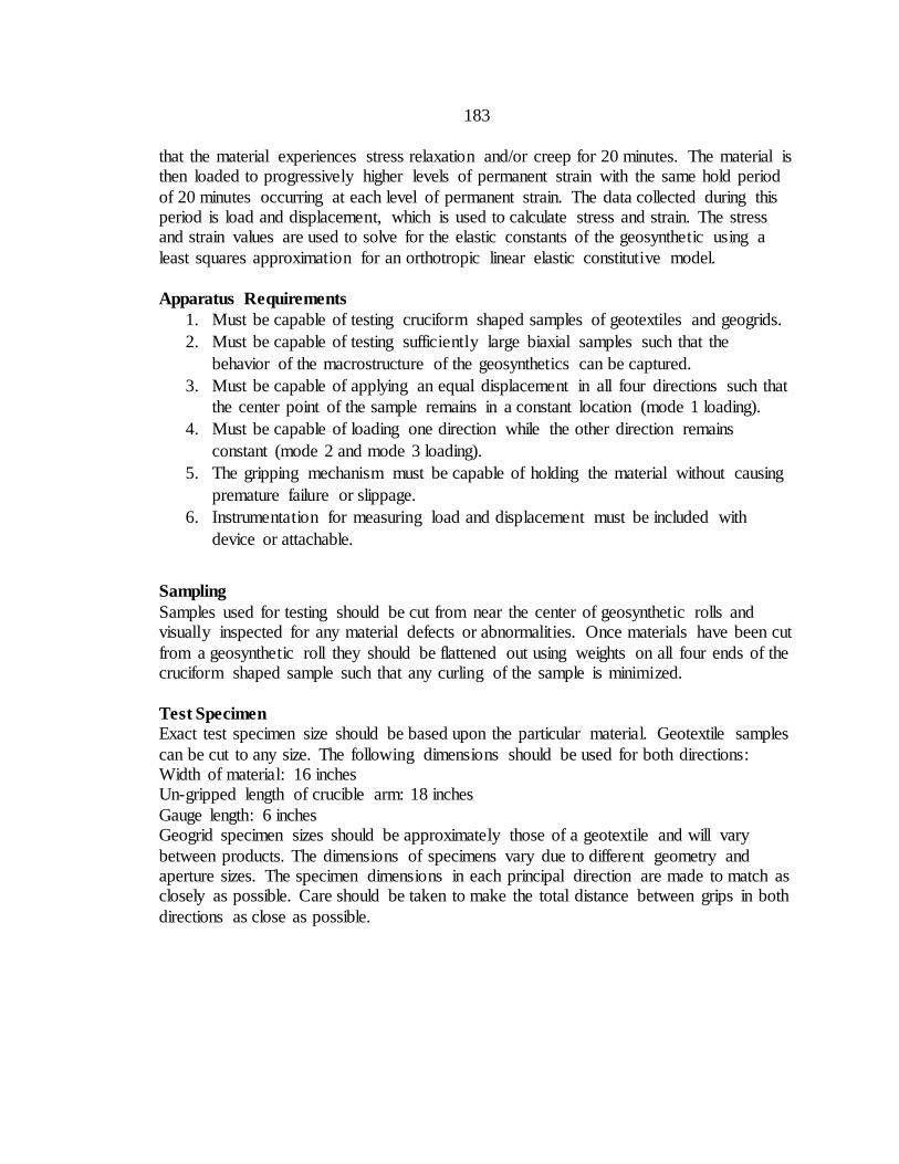
183
that the material experiences stress relaxation and/or creep for 20 minutes. The material is then loaded to progressively higher levels of permanent strain with the same hold period
of 20 minutes occurring at each level of permanent strain. The data collected during this period is load and displacement, which is used to calculate stress and strain. The stress and strain values are used to solve for the elastic constants of the geosynthetic using a
least squares approximation for an orthotropic linear elastic constitutive model.
Apparatus Requirements
1. Must be capable of testing cruciform shaped samples of geotextiles and geogrids.
2. Must be capable of testing sufficiently large biaxial samples such that the
behavior of the macrostructure of the geosynthetics can be captured.
3. Must be capable of applying an equal displacement in all four directions such that
the center point of the sample remains in a constant location (mode 1 loading).
4. Must be capable of loading one direction while the other direction remains
constant (mode 2 and mode 3 loading).
5. The gripping mechanism must be capable of holding the material without causing
premature failure or slippage.
6. Instrumentation for measuring load and displacement must be included with
device or attachable.
Sampling
Samples used for testing should be cut from near the center of geosynthetic rolls and visually inspected for any material defects or abnormalities. Once materials have been cut
from a geosynthetic roll they should be flattened out using weights on all four ends of the cruciform shaped sample such that any curling of the sample is minimized.
Test Specimen
Exact test specimen size should be based upon the particular material. Geotextile samples
can be cut to any size. The following dimensions should be used for both directions: Width of material: 16 inches Un-gripped length of crucible arm: 18 inches
Gauge length: 6 inches Geogrid specimen sizes should be approximately those of a geotextile and will vary
between products. The dimensions of specimens vary due to different geometry and aperture sizes. The specimen dimensions in each principal direction are made to match as closely as possible. Care should be taken to make the total distance between grips in both
directions as close as possible.
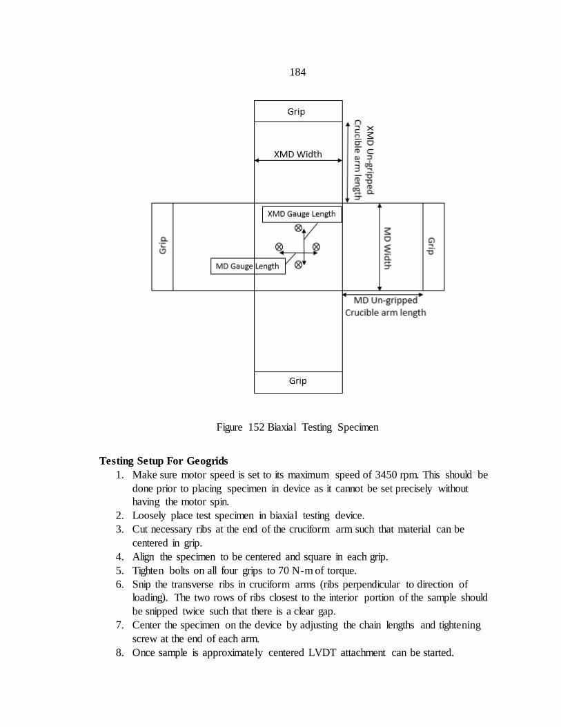
184
Figure 152 Biaxial Testing Specimen
Testing Setup For Geogrids
1. Make sure motor speed is set to its maximum speed of 3450 rpm. This should be
done prior to placing specimen in device as it cannot be set precisely without
having the motor spin.
2. Loosely place test specimen in biaxial testing device.
3. Cut necessary ribs at the end of the cruciform arm such that material can be
centered in grip.
4. Align the specimen to be centered and square in each grip.
5. Tighten bolts on all four grips to 70 N-m of torque.
6. Snip the transverse ribs in cruciform arms (ribs perpendicular to direction of
loading). The two rows of ribs closest to the interior portion of the sample should
be snipped twice such that there is a clear gap.
7. Center the specimen on the device by adjusting the chain lengths and tightening
screw at the end of each arm.
8. Once sample is approximately centered LVDT attachment can be started.
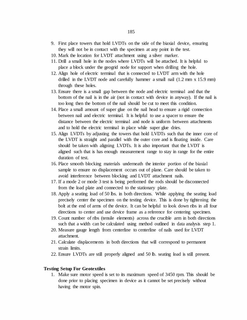
185
9. First place towers that hold LVDTs on the side of the biaxial device, ensuring
they will not be in contact with the specimen at any point in the test.
10. Mark the location for LVDT attachment using a silver marker.
11. Drill a small hole in the nodes where LVDTs will be attached. It is helpful to
place a block under the geogrid node for support when drilling the hole.
12. Align hole of electric terminal that is connected to LVDT arm with the hole
drilled in the LVDT node and carefully hammer a small nail (1.2 mm x 15.9 mm)
through these holes.
13. Ensure there is a small gap between the node and electric terminal and that the
bottom of the nail is in the air (not in contact with device in anyway). If the nail is
too long then the bottom of the nail should be cut to meet this condition.
14. Place a small amount of super glue on the nail head to ensure a rigid connection
between nail and electric terminal. It is helpful to use a spacer to ensure the
distance between the electric terminal and node is uniform between attachments
and to hold the electric terminal in place while super glue dries.
15. Align LVDTs by adjusting the towers that hold LVDTs such that the inner core of
the LVDT is straight and parallel with the outer core and is floating inside. Care
should be taken with aligning LVDTs. It is also important that the LVDT is
aligned such that is has enough measurement range to stay in range for the entire
duration of test.
16. Place smooth blocking materials underneath the interior portion of the biaxial
sample to ensure no displacement occurs out of plane. Care should be taken to
avoid interference between blocking and LVDT attachment nails.
17. If a mode 2 or mode 3 test is being performed the rods should be disconnected
from the load plate and connected to the stationary plate.
18. Apply a seating load of 50 lbs. in both directions. While applying the seating load
precisely center the specimen on the testing device. This is done by tightening the
bolt at the end of arms of the device. It can be helpful to look down ribs in all four
directions to center and use device frame as a reference for centering specimen.
19. Count number of ribs (tensile elements) across the crucible arm in both directions
such that a width can be calculated using method outlined in data analysis step 1.
20. Measure gauge length from centerline to centerline of nails used for LVDT
attachment.
21. Calculate displacements in both directions that will correspond to permanent
strain limits.
22. Ensure LVDTs are still properly aligned and 50 lb. seating load is still present.
Testing Setup For Geotextiles
1. Make sure motor speed is set to its maximum speed of 3450 rpm. This should be
done prior to placing specimen in device as it cannot be set precisely without
having the motor spin.
186
2. Loosely place test specimen in biaxial testing device.
3. Melt holes at ends of crucible arms so that bolts on grips fit through the specimen
and it is centered and square in the grip.
4. Tighten bolts on all four grips to 70 N-m of torque.
5. Cut 11 slits of equal width along the crucible arms in the direction being loaded.
6. Center the specimen on the device by adjusting the chain lengths and tightening
screw at the end of each arm.
7. Once sample is approximately centered LVDT attachment can be started.
8. First place towers that hold LVDTs on the side of the biaxial device, ensuring
they will not be in contact with the specimen at any point in the test.
9. Mark the location for LVDT attachment using a silver marker.
10. Push the sharp threaded rod through woven fibers at the marked locations.
11. Place a nut above and below the geotextile on the threaded rod and tighten against
each other to ensure a rigid connection.
12. Align LVDTs by adjusting the towers that hold LVDTs such that the inner core of
the LVDT is straight and parallel with the outer core and is floating inside. Care
should be taken with aligning LVDTs. It is also important that the LVDT is
aligned such that it has enough measurement range to stay in range for the entire
duration of test.
13. Place smooth blocking materials underneath the interior portion of the biaxial
sample to ensure no displacement occurs out of plane. Care should be taken to
avoid interference between blocking and LVDT attachment rods.
14. If a mode 2 or mode 3 test is being performed the rods should be disconnected
from the load plate and connected to the stationary plate.
15. Apply a seating load of 50 lbs. in both directions and while doing this precisely
center the specimen on the testing device. This is done by tightening the bolt at
the end of arms of the device. It can be helpful to look down fibers in all four
directions to center and use device frame as a reference for centering specimen.
16. Measure width of sample gripped.
17. Measure gauge length from centerline to centerline of rods.
18. Calculate displacements in both directions that will correspond to permanent
strain limits.
19. Ensure LVDTs are still properly aligned and 50 lb. seating load is still present.
Testing Procedure
1. Make sure motor speed dial is set to its maximum speed of 3450 rotations per
minute.
2. Make sure displacement values corresponding to permanent strain values are
known.
3. Reset the data logging device (resend program) so that data being collected starts
from scratch.
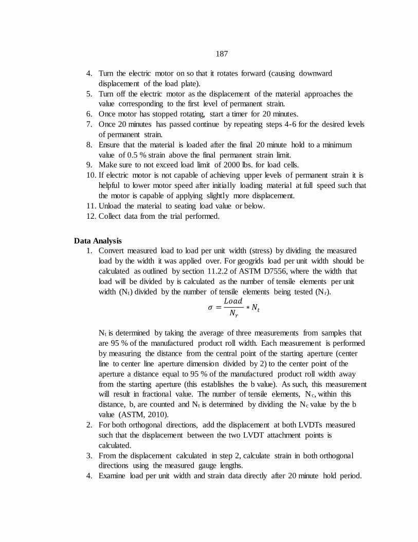
187
4. Turn the electric motor on so that it rotates forward (causing downward
displacement of the load plate).
5. Turn off the electric motor as the displacement of the material approaches the
value corresponding to the first level of permanent strain.
6. Once motor has stopped rotating, start a timer for 20 minutes.
7. Once 20 minutes has passed continue by repeating steps 4-6 for the desired levels
of permanent strain.
8. Ensure that the material is loaded after the final 20 minute hold to a minimum
value of 0.5 % strain above the final permanent strain limit.
9. Make sure to not exceed load limit of 2000 lbs. for load cells.
10. If electric motor is not capable of achieving upper levels of permanent strain it is
helpful to lower motor speed after initially loading material at full speed such that
the motor is capable of applying slightly more displacement.
11. Unload the material to seating load value or below.
12. Collect data from the trial performed.
Data Analysis
1. Convert measured load to load per unit width (stress) by dividing the measured
load by the width it was applied over. For geogrids load per unit width should be
calculated as outlined by section 11.2.2 of ASTM D7556, where the width that
load will be divided by is calculated as the number of tensile elements per unit
width (Nt) divided by the number of tensile elements being tested (N r).
𝜎 =𝐿𝑜𝑎𝑑
𝑁𝑟
∗ 𝑁𝑡
Nt is determined by taking the average of three measurements from samples that
are 95 % of the manufactured product roll width. Each measurement is performed
by measuring the distance from the central point of the starting aperture (center
line to center line aperture dimension divided by 2) to the center point of the
aperture a distance equal to 95 % of the manufactured product roll width away
from the starting aperture (this establishes the b value). As such, this measurement
will result in fractional value. The number of tensile elements, Nc, within this
distance, b, are counted and Nt is determined by dividing the Nc value by the b
value (ASTM, 2010).
2. For both orthogonal directions, add the displacement at both LVDTs measured
such that the displacement between the two LVDT attachment points is
calculated.
3. From the displacement calculated in step 2, calculate strain in both orthogonal
directions using the measured gauge lengths.
4. Examine load per unit width and strain data directly after 20 minute hold period.
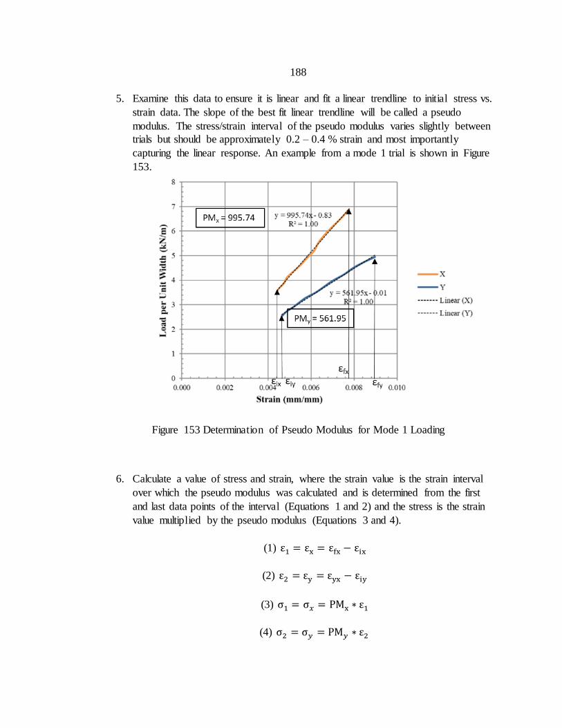
188
5. Examine this data to ensure it is linear and fit a linear trendline to initial stress vs.
strain data. The slope of the best fit linear trendline will be called a pseudo
modulus. The stress/strain interval of the pseudo modulus varies slightly between
trials but should be approximately 0.2 – 0.4 % strain and most importantly
capturing the linear response. An example from a mode 1 trial is shown in Figure
153.
Figure 153 Determination of Pseudo Modulus for Mode 1 Loading
6. Calculate a value of stress and strain, where the strain value is the strain interval
over which the pseudo modulus was calculated and is determined from the first
and last data points of the interval (Equations 1 and 2) and the stress is the strain
value multiplied by the pseudo modulus (Equations 3 and 4).
(1) ε1 = εx = εfx − εix
(2) ε2 = εy = εyx − εiy
(3) σ1 = σ𝑥 = PMx ∗ ε1
(4) σ2 = σ𝑦 = PM𝑦 ∗ ε2
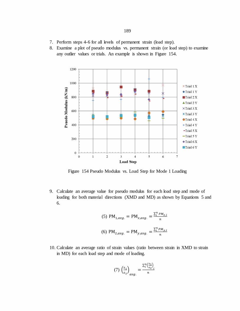
189
7. Perform steps 4-6 for all levels of permanent strain (load step).
8. Examine a plot of pseudo modulus vs. permanent strain (or load step) to examine
any outlier values or trials. An example is shown in Figure 154.
Figure 154 Pseudo Modulus vs. Load Step for Mode 1 Loading
9. Calculate an average value for pseudo modulus for each load step and mode of
loading for both material directions (XMD and MD) as shown by Equations 5 and
6.
(5) PM1,𝑎𝑣𝑔. = PM𝑥,𝑎𝑣𝑔. =∑ 𝑃𝑀𝑥 ,𝑖
𝑛𝑖
𝑛
(6) PM2,𝑎𝑣𝑔. = PM𝑦,𝑎𝑣𝑔. =∑ 𝑃𝑀𝑦,𝑖
𝑛𝑖
𝑛
10. Calculate an average ratio of strain values (ratio between strain in XMD to strain
in MD) for each load step and mode of loading.
(7) (ε1
ε2)
𝑎𝑣𝑔.
=∑ (
ε1ε2
)𝑖
𝑛𝑖
𝑛
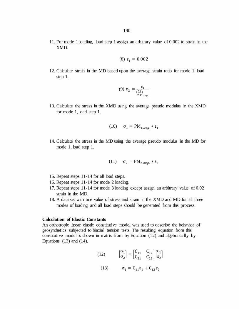
190
11. For mode 1 loading, load step 1 assign an arbitrary value of 0.002 to strain in the
XMD.
(8) ε1 = 0.002
12. Calculate strain in the MD based upon the average strain ratio for mode 1, load
step 1.
(9) ε2 =ε1
(ε1ε2
)𝑎𝑣𝑔.
13. Calculate the stress in the XMD using the average pseudo modulus in the XMD
for mode 1, load step 1.
(10) σ1 = PM1,𝑎𝑣𝑔. ∗ ε1
14. Calculate the stress in the MD using the average pseudo modulus in the MD for
mode 1, load step 1.
(11) σ2 = PM2,𝑎𝑣𝑔. ∗ ε2
15. Repeat steps 11-14 for all load steps.
16. Repeat steps 11-14 for mode 2 loading.
17. Repeat steps 11-14 for mode 3 loading except assign an arbitrary value of 0.02
strain in the MD.
18. A data set with one value of stress and strain in the XMD and MD for all three
modes of loading and all load steps should be generated from this process.
Calculation of Elastic Constants
An orthotropic linear elastic constitutive model was used to describe the behavior of geosynthetics subjected to biaxial tension tests. The resulting equation from this constitutive model is shown in matrix from by Equation (12) and algebraically by
Equations (13) and (14).
(12) [σ1
σ2] = [
C11 C12
C21 C22] [
ε1
ε2]
(13) σ1 = C11ε1 + C12ε2
191
(14) σ2 = C21ε1 + C22ε2
Constants C11, C12, C21 and C22 are defined by Equations (15), (16), (17) and (18)
(15) C11 =E1
1−ν12ν21
(16) C22 =E2
1−ν12ν21
(17) C12 =ν21E1
1−ν12ν21
(18) C21 =ν12E2
1−ν12ν21
The major and minor Poisson’s ratio terms are related by Equation (19) and constrained
by Equation (20).
(19) ν12 = ν21 E1
E2
(20) ν12ν21 < 1
A least squares approximation is used to solve for the elastic constants of geosynthetics using the data generated from biaxial tests. The least squares approximation can be
performed as a stress or strain minimization. Reported values for elastic constants should be an average of the value obtained from stress and strain minimizations. The process for
calculating elastic constants using a stress minimization is shown by Equations (21) through (27).
(21) S = ∑{(C11ε1 + C12ε2 − σ1)2 + (C21ε1 + C22ε2 − σ2)
2}
(22) ∂S
∂C11=
∂S
∂C22=
∂S
∂C12= 0
(23) [
∑(ε12) ∑(ε1ε2) 0
∑(ε1ε2) ∑(ε22 + ε1
2) ∑(ε1ε2)
0 ∑(ε1ε2) ∑(ε22)
] [
C11
C12
C22
] = [
∑(σ1ε1)
∑(σ1ε2 + σ2ε1)
∑(σ2ε2)]
(24) E2 = C22 −C12
2
C11
192
(25) ν12 = [C11
C22(1 −
E2
C22)]
0.5
(26) E1 =ν122 E2
1−E2C22
(27) ν21 = ν12 E2
E1
For a strain minimization Equations (13) and (14) are rearranged in terms of strain as
defined in Equations (28) and (29).
(28) ε1 =σ1
E1−
σ2
E2ν21
(29) ε2 =σ2
E2−
σ1
E1ν12
Constants are defined by Equations (30) through (32)
(30) E11 =1
E1
(31) E22 =1
E2
(32) E12 =ν12
E1 = E21 =
ν21
E2
Least Squares is applied in a similar manner as for the stress minimization as shown in
Equations (33) through (35). The elastic constants are calculated using Equations (36)
through (39).
(33) S = ∑[{(E11σ1 − E12σ2) − ε1}2 + {(E22σ2 − E12σ1) − ε2}
2]
(34) ∂S
∂E11=
∂S
∂E22=
∂S
∂E12= 0
(35) [
∑(σ12) ∑(−σ1σ2) 0
∑(−σ1σ2) ∑(σ22 + σ1
2) ∑(−σ1σ2)
0 ∑(−σ1σ2) ∑(σ22)
] [
𝐸11
E12
E22
] = [
∑(σ1ε1)
∑(−σ1ε2 − σ2ε1)∑(σ2ε2)
]
193
(36) E1 =1
E11
(37) E2 =1
E22
(38) ν12 = E1 ∗ E12
(39) ν21 = ν12 E2
E1
The elastic constants are calculated at each load step using the data set of stress and strain
values from all three modes of loading for that given load step as described in Step 19 in
the Data Analysis section. If a single set of elastic constants is desired then data sets from
all load steps should be combined.
Recommended


![Index [rd.springer.com]978-1-4419-6312-3/1.pdf · Elastic deformation elastic constants (see Elastic constants) generalized Hooke’s law, 173 linear elasticity, 15, 25 strain energy,](https://img.pdfslide.us/doc/110x75/5e349187dde0ff2df4470398/index-rd-978-1-4419-6312-31pdf-elastic-deformation-elastic-constants-see.jpg)