Working Paper
March 20, 2011
Determinants of Comparative Advantage in Services
Erik van der Marel* Sciences‐Po
Abstract
This paper analyzes whether and to what extent determinants of comparative advantage have explanatory power for conventional services trade. It assesses the geographical, Heckscher‐Ohlin and institutional determinants of services trade based on the literature for goods trade. Moreover, this paper investigates the importance of a country’s governance of regulation as a source of comparative advantage in services markets. Determinants for services trade differ from goods. Services trade is more sensitive to a country’s stock of high‐skilled and mid‐skilled labour, more receptive to the level of trust enjoyed by any importers, and more dependant on the quality of regulatory governance practiced when liberalizing services sectors. The counterfactual analyses presented in this paper show furthermore that these factors when affected by policy can bring substantial gains to countries. Specifically, countries with already good regulatory governance structures would enjoy relatively higher growth share in services trade by capitalizing on their high‐skilled stock. Other countries, however, would instead to better by improving their condition of regulatory governance. JEL Codes: F13; L8 ; F15. Key words: Trade in services; Comparative advantage, Institutions; Regulation.
* Research Fellow at the Groupe d’Economie Mondiale (GEM) at Sciences Po. Please send comments to erik.vandermarel@sciences‐po.org. The author wishes to thank Bernard Hoekman, Patrick Messerlin, Ben Shepherd, Sébastien Miroudot, Davin Chor, Marc Melitz and Alexandre Levernoy for very valuable comments and suggestions when writing this paper.

2
1 Introduction The concept of comparative advantage in international trade initially developed by Ricardo has been a fundamental starting point in trade economics for theoretical and empirical work. Eaton and Kortum (2002) led to a resurgence of this theory and empirical research has subsequently developed into the institutional structure of comparative advantage such as Levchenko (2007) and Nunn (2007) on contract enforcement and Costinot (2009) on human capital.1 A recent paper by Chor (2010) incorporates Heckscher‐Ohlin forces as an additional source of comparative advantage by way of including Romalis’ (2004) methodology of factor proportions within a common framework founded on an extended Eaton‐Kortum model.
A lot of these works have focused on goods trade. We lack any rigorous empirical understanding of the determinants of comparative advantage in services trade. This is in sharp contrast to current patterns of trade where the role services has demanded an ever increasing importance. Particularly in developed OECD countries where services trade take up on average almost 25 of their national output.2 This paper empirically extends Chor (2010) by taking services as the focal point of research in order to assess the geographical, factor, institutional and regulatory determinants of comparative advantage in services trade. The bulk of services trade takes place among the OECD economies as Table 1 suggests. While these economies thus have a revealed comparative advantage in services, it leaves unexploited why these countries are better capable of exporting services. In other words, what do services require to be successfully traded, particularly compared to goods?
Such analysis is crucial not only from an academic perspective but also from a policy point of view. Much of the academic literature supposes that services are no different than goods. By quantifying the sources of comparative advantage in services and then focussing on the systematic differences of services compared to goods, this paper assesses whether this implicit assumption in the literature – structure of comparative advantage are the same – is supported by the data. As for policy, to know where differences in sources of comparative advantage come from would also facilitate formulating policy responses that go beyond demand management mechanisms. For example, improving developed economies’ current account imbalance through expanding the scope for international trade in services has recently put forward as an alternative policy initiative for rebalancing the global economy. (See for example, Claessens, Evenett and Hoekman, 2010).
This paper contributes to the existing empirical literature on the comparative advantage in services in a number of ways. First, there is reason to believe that human capital is especially important for comparative advantage in services (Hoekman and Mattoo, 2008). However, in contrast to what is often claimed in literature, high‐skilled factor intensities differ greatly among services. Construction, transport and storage services, but also telecommunication services require far less high‐skilled labor than some business services. These differences in services factor requirements are also present among countries as shown in Table 1 and should effect their services export structures and hence comparative advantage. By taking both mid and high‐skilled labour in our analysis, this paper also investigates to what extent mid‐skilled labour forms a determinant for services trade.
Second, recent empirical works by Levchenko (2007) and Nunn (2007) suggest that industries which are respectively more dependent on contract enforcement and more relationship specific
1 Other studies that develop institutional structure of comparative advantage include Cuñat and Melitz (2007) on labor
market flexibility, and finally Beck (2003) and Manova (2008) on financial development. 2 This number is the average of all countries selected in this paper’s sample over the years 1999 to 2005. Large differences
remain. The US shows a percentage of around 5% whereas on average (excl. Luxembourg) European countries show an average of 20%. Column 2 of Table 1 shows the average of each sector’s services trade value divided by their sectoral output, by country. Moreover, especially for developing countries services trade is considered as a development tool, which even more importantly, puts forward the question what actually determines comparative advantage in services. See e.g. Ghani and Kharas, (2010), Mattoo and Payton (2007), Mattoo, Stern and Zanini (2008).

3
require good rule of law. Institutions should also matter for services.3 Services are often very differentiated as a result of the structure of joint production and consumption. Moreover, the intangibility of services implies that other types of institutions may determine comparative advantages such as the level of trust acquired from a partner country.4 This paper takes these issues into account by extending Levchenko’s and Nunn’s empirical work for services. Evidence on the link between institutions and services trade is, however, broad‐based and largely anecdotal. Most papers put this link in connection with developing countries so that such outcome is rather predictable as services trade increases with economic development.
Third, the characteristics of services markets often result in extensive regulation. Differences in regulation across countries should affect trade. This paper also takes into account deregulation in combination with good governance as a source of comparative advantage in services; in line with theory developed by Copeland and Mattoo (2008). Moreover, these regulatory institutions can be organised in a specific geographical setting, which in turn constitutes a source of services trade. To date no rigorous empirical understanding has been undertaken to verify in how far liberalised services markets need a specific type of regulatory environment on which services exporters can capitalize.
The paper is organized as follows. Section 2 provides a theoretical framework according to the model of comparative advantage developed by Eaton and Kortum (2002) and extended by Chor (2010). Section 3 sets out the empirical specification which will then be estimated using OLS and other techniques to take into account zero‐trade flows in services. Section 4 goes deeper into analyzing the differences between services and goods when measuring the determinants of comparative advantage. Consequently, section 5 provides an alternative way of showing the estimated coefficients for goods and services using counterfactuals. Last, a conclusion will be given at he end of the paper. 2 Theoretical Environment The model presented in this section provides a framework for the empirical analysis and draws heavily on Eaton and Kortum (2002) and on Chor (2010). The latter extends the Eaton and Kortum model by including interaction terms for factor prices and institutional productivity. These interactions represent measures of comparative advantage which in turn consist of Heckscher‐Ohlin, institutional and regulatory determinants of comparative advantage. In this paper, the explanation of the model is set out in a sectoral context so as to include services only. 2.1 Benchmark Model for Services Data The economy consists of D countries, indexed by d = 1,…, D (a country can be indexed by either o or d). Furthermore, there are S sectors that represent all services that an economy produces, indexed by 3 Such evidence is currently based on Amin and Mattoo (2006) who show that across Indian states services output per
capita is strongly associated with relatively stronger institutions. The authors state that this is, for example, reflected by the transmission and distribution losses of the public sector electricity providers. See also Hoekman and Matoo (2008). This paper goes a step further in analysing the interaction of country and sectoral institutional forces that may cause countries to have greater services exports.
4 For example, see Lennon (2007) which concludes that sources of services trade is distinguished from goods trade. Moreover, in the public policy/ international relations literature there is a separate ongoing debate about the level of trust with regards to the type of services liberalisation and regulation. See, e.g. Nicolaidis (2007) and Nicolaidis and Schmidt (2007).

4
s = 0, 1,…, S. Here, only the services sectors (s ≥ 1) are tradable whilst sector 0 indicates the non‐tradable service sector.5 For each of these service sectors (s ≥ 1) a continuum, with mass normalized to one, of differentiated variety is available, indexed by js ∈ (0,1). Whereas the model is static, the dataset we have collected consist of 7 years, the model is static and subsequently time subscripts in the equations will be suppressed.6 As well, the model refers to individual varieties which in the empirical part will be replaced by individual services sectors. Consumer Preferences Each country d has a mass of identical consumers, which is normalized to one, each of whom owns all factors of production. As in Donaldson (2010), we assume the continuum of differentiated varieties j to come from one sector s. Total utility is a Cobb‐Douglas collection over the consumption of goods and services produced by sector s with a constant elasticity of substitution function over the consumption of each variety js within each sector. Therefore, the log utility function of a consumer in country d is:
lnUd = (1η) lnQnd + η Σs≥1 (μ / εs) ln ∫(Qds(j)εsdj, (1)
where Qds (j) is the quantity of variety js from sector s consumed in country d, εs = (σs – 1) / σs, where σs is the constant elasticity of substitution, and Σs µs = 1. Note that Qnd (j) is the non‐tradable service sector while the share of income spent on tradables is equal to η ∈ (0,1). All agents within country d charge a cost price of cd per unit for bringing in their factors of production, called together Fd. Consumers maximize their utility by using their income that is at their disposal after incurring the cost of the all factors of production, which is cdFd. Production and Market Structure Each variety j of each sector s is produced in a perfectly competitive framework using constant returns to scale production technology. Let zos(j) denote the amount of variety j of sector s that can be produced in country o,7 which in Eaton and Kortum (2002) is the realization of a stochastic variable Zos drawn from a Type‐I (Gumbel) extreme value distribution, i.e. the productivity distribution. The productivity differences across countries and sectors is summarized by the parameters of the distribution, which gives:
Fos(z) = Pr[Zos ≤ z] = exp (– ψos z –θs) (2) where the distributions are independent across variety, services and country. ψos > 0 governs the state of technology in country o for a specific sector s whilst θs > 0 governs the variation of
5 Despite the fact that a large part of the services sectors remain non‐tradable, such as to a large extent the personal
services sector, these services are nevertheless becoming tradable. An example of such non‐tradable becoming tradable is when people are travelling abroad to undergo treatments by, e.g. hairdressers, surgeons, or even elderly care can be provided by foreign suppliers. On the other hand, some personal services are likely to remain nationally supplied. The data on the personal services are rather scare and will therefore automatically to a large extent left out in the analysis.
6 Therefore, in contrast to former studies which have dealt with empirical measures of comparative advantage we treat the variables that determine comparative advantage as country‐sector‐year specific.
7 For clarity, country d is the importing country and country o is the exporting country.

5
productivity in sector s for any country o. The former can be seen as the country’s absolute advantage, the latter represents Ricardian productivity, i.e. comparative advantage. In the empirical part of this paper we have data on both country and sector level which represent absolute and comparative advantage respectively. However, it is the interaction between sector and country attributes that will reveal the true the force of comparative advantage in services.8
Before trade takes place, producers which have access to the technology in equation (2) calculate costs of a particular service variety by poos = co / zos(j), where cos denotes the unit costs that agents charge for bringing in their factors of production F, in this case labor and capital, to produce any service. Services Trade Costs Before services became tradable, consumers in country d had the only possibility to consume the non‐tradable service for which their country could have the worst draw from the productivity distribution in equation (2). Now services have become tradable, it gives the consumers the opportunity to consume the varieties from abroad for which its exporters enjoys a superior productivity draw. This results in that the producers of this variety specialise for which they receive the best productivity draw. Each country o holds potential producers that can supply and export a sector variety s. However, to export services costs must be incurred. At the one hand, these costs cover transportation costs that can be considerably low for cross‐border services trade.9 On the other hand, they also include other barriers to trade which can be considerably higher for services if one takes into account all non‐tariff and regulatory restrictions.10
Standard practice in trade literature is to conveniently use Samuelson’s (1954) iceberg transport costs to cover such geographic or other natural non‐tariff barriers. For one unit of service to be traded from country o to country d, these costs can be modelled as Bods ≥ 1 units of a service that must be produced and sent in country o.11 The iceberg costs can vary considerably for services as some services can be easily tradable (e.g. Mode 1 cross‐border trade over the internet), whilst for other services (such as through Mode 2 where the consumer moves) it is more costly to trade.12 Moreover, one assumes to satisfy the usual property of Bods ≤ Boks, Bkds, which means that it is always less costly to send services directly from country o to country d, rather than via a third country k. Services Prices The price of an identical services variety in country o differs from the price in country d because the above mentioned trade costs need to be incurred. Let pods (j) denote the price of variety j of service s produced in country o, but send to country d for consumption there. This gives:
8 This distinction of productivity will also come out in my counterfactual analysis where we treat the sector and country
variables as respectively comparative and absolute advantage. 9 The Generally the General Agreement of Trade in Services (GATS) within the WTO defines four modes of supply in
international services trade. Mode 1 covers cross‐border trade with services supplied from the territory of one country into the territory of another, which largely takes place over the internet, Mode 2 defines trade as consumption abroad with services supplied in the territory of a country to the consumers of another (i.e. tourism), Mode 3 measures trade through ccommercial presence with services supplied through any type of business or professional establishment of one country in the territory of another or, more precisely, sales of foreign firm affiliates, and finally Mode 4 trade deals with temporary movement of labour, i.e. presence of natural persons with service supplied by nationals of a country in the territory of another workers abroad. This paper only takes into account trade through Mode 1 and 2 and hence leaves out all other types of services trade that additionally could take place as described in the GATS.
10 Of note, by focussing on services trade through Mode 1 as established in the GATS we ignore services trade through Mode 3 where fixed (entry) costs play a much larger role. Note furthermore that complementarities between cross‐border trade and trade through commercial presence appear to exist, see for instance Lennon (2009) and Fillat‐Cateljón, Francois and Woerz (2009). In this paper, these complementarities will to some extent taken into account.
11 No trade costs are incurred when Bods = 1, Furthermore, Boos = 1 if normalized. 12 As well here, some services are still surrounded by higher levels of regulatory protection or other non‐regulatory non‐
tariff barriers. Moreover, services data in the empirical part covers Mode 1 and 2. As stated, Mode 2 trade can constitute considerable transport costs since this mode of trade considers a consumer to move to the country of recipient.
6
pods(j) = Bodspoos(j) = cosBods/zos(j) (3)
where cos denotes the unit production costs for a service sector s to be made by a prospective exporter, country o. Following Chor (2010), we specify factor price terms in order to incorporate the role of Heckscher‐Ohlin forces of comparative advantage through production cost differences between country o and d based on each of their endowment structures. More precisely, there are F factors of production, indexed by f = 0, 1, …, F. Furthermore, the unit production cost is cos that is a Cobb‐Douglas aggregate over factor prices in country o, so that we get cos = ПFf=0(wof)Posf. Here, wof is the price of factor f in country o while posf ∈ (0,1) is the share of total payments in service sector s, also in country o, that goes to agents who offer a particular factor. Moreover, under constant returns to scale the following condition holds ΣFf=0posf = 1.13 This interaction makes clear how well services firms can make use of country o’s factor attributes such as the amount of skilled labour or capital and so can raise this country’s productivity. Hence, for any lower value of cos and Bos, services prices will tend to decrease. Services Productivity As in goods trade, the probability of enjoying increased exports in service sectors depends on the productivity level, here zos(j). The realization of this productivity term depends on a fine interplay between sector and country characteristics. To the extent that producers within country o can successfully export their services depends again on how well they are able to capitalize on country o’s attributes that is precisely necessary for the service to be exported. For example, after deregulation in a particular services sector has taken place, the ability to successfully export by services producers depends on how well domestic (regulatory) institutions govern these deregulated markets in terms of private sector development. Countries where these institutions are more efficient are expected be more productive services sectors because they will become more institutionally dependant on good policy (i.e. re‐regulation). These and other institutional determinants of services will be specified as follows:
lnzos(j) = Σ{cs}β1CoSs + γo + γs + β0εos(j) (4)
which states the productivity on logs of country o in variety j in sector s. Formally, in equation (4) Coc and Sss represent through the interaction term the realization of increased productivity in country o’s for service sector variety s. The term β0εos(j) deals with the possibility that a country with on average a lower rate of productivity for its service sectors can nevertheless be an exporter due to a positive productivity shock. Therefore, εos(j) is a stochastic term and are the independent draws from the Type 1 (Gumbel) extreme‐value distribution that affects zos(j) directly. The parameter β0 regulates the variance of these productivity shocks. Furthermore, γo and γs in the equation are respectively the exporter and sector fixed effects. 13 As stated in Chor (2010), each firm takes the wof as given as they are too small to influence aggregate factor markets.
Moreover, such model does not imply factor price equalization across countries due to the presence of productivity differences and transport costs.

7
Equilibrium Prices Consumers in country d are indifferent about where to buy a given service variety j. Yet they are only interested in buying the variety from country o if this country actually offers the variety at the lowest cost, which can be formalized by pds(j) = min{pods(j): i = 1,…N}. Therefore, the equilibrium price needs to be solved by taking into account the stochastic term of the productivity shock εos(j) in equation (4) that directly affects prices pods(j) of a particular service variety and that enables the service variety subsequently to be exported from country o to d. Given that the productivity term in equation (4) zos(j) is drawn through εos(j) from the cumulative distribution function (CDF) in equation (2), pods(j) is therefore the realization of a random variable Pods(j) drawn from the CDF:
Gods(p) = Pr(Pods ≤ p) = 1 – exp[ – (cosBods)‐θpθψos] (5) where ψos = exp{ θΣ{cs}βciCocSss + θγo + θγs } and θ = 1/β0, which inversely regulates the variance of productivity shocks of each comparative advantage determinant in each services sector s around its average.14 Equation (5) is the price distribution for variety j in service sector s in country o that is presented to country d, but is not actually bought yet. Consumption of a particular service variety j will only happen in country d when the price distribution is the lowest among all countries N, which is therefore also given in a CDF form called Gos(p) and which can be given as follows:
Gds = 1 – ΠDO=1 [1 – Gods(p)],
= 1 – exp( – [ΣDO=1(cosBods) ‐θψos] pθ)
This price distribution has some important properties. One of them is that one can now calculate the price index for the CES function. That is to say, one can now calculate any moment of the prices of interest given the price distribution of the actual prices paid by consumers in country d. Hence, the price index that is expected – or the expected value of the equilibrium price – of any variety j of service sector s found in country d is the following:
E[pds(j)] = Pds = ωs[ΣDO=1(cosBods) ‐θψos]‐1/θ (6) where ω = Γ[(θ+1‐σ/θ)] and Γ is the Gamma function. In the empirical part the observed prices for the services sectors that we will use are collected by statistical agencies, in this case the OECD. These prices will be used for these expected prices.
14 Since equation (5) states the distribution of a price, consumers in country d face a price that is presented by country o for
variety j in service sector s by substituting equation (4) into (5), which gives the following result in logs: lnpods(j) = ln(cosBods) ‐ γo + γs ‐ Σβ1CoSs ‐ β0εos(j). From the term on the right‐hand side it becomes clear that in increase in factor costs and natural barriers increases the price of a service, whereas a higher productivity draw lowers the service price for variety j. Note furthermore that in the empirical part the inverse parameter spread θ for each comparative advantage determinant will be suppressed in each estimation equation.

8
Services Trade Flows A second property from the price distribution that derives directly from the model developed by Eaton and Kortum (2002) is that the price distribution for the services sector variety as given in equation (5) actually purchased by country d from any country o has a similar price distribution, which can be formalized as ∀o Pr [Pds < p | Pds = Pods] = Gds(p). A service imported from a different source has no affect on the price of a purchased service in country d. This property implies that the probability that country d imports the service at the lowest price from any country o can be summarized as follows:
πods = Pr[Pod(j) ≤ min{Pod(j), s ≠ o}]
= (coBods)θψos / Σok=1(cksBkds)θψks (7)
This property of πods combined with a same price distribution for each exporting country o leads to the immediate corollary that the average expenditure per service variety s of the importing country d does not vary among any exporting country o. The fraction that consumers in country d spend on buying a service variety s from country o, that is Xods, must be equal to the fraction of these consumers’ expenditure on all services from all countries o, which is Xds. Aggregating trade flows therefore entails that:
πods = Xod / Xd
= (coBods)‐θψos / ΣDk=1(cksBkds) ‐θψks = ωsθ(cosBods) ‐θψos(pds)θ (8) where the last expression on the right‐hand side makes use of the price index given in equation (6). It states that the share that consumers spend on imports of services s from country o is exactly πods. By the same token, it indicates to what extent country o is able to exploit comparative advantage in a particular services variety s. This depends in turn on how well services firms can make use of country o’s favourable conditions that the service variety particularly requires. 3 Empirical Step 1: OLS, zerotrade flows and Poisson In what follows we set out the estimated equation and explain briefly the motivations and definitions of the selected variables. Then we will analyze the OLS results and other estimations techniques such as Poisson to deal with zero trade flows. The estimated equation follows standard practice in literature by incorporating geographical trade barriers, Heckscher‐Ohlin and institutional forces, but is extended with data from input‐output tables, data on sectoral factor intensities and country factor endowments. Moreover, sectoral regulatory reform and national governance variables are also included. All of these are original and appropriate for services trade.

9
3.1 Empirical Strategy Our starting point is to acquire empirical measures of the variables as presented in the model. We apply standard practice for the dyadic geographical variables that can be found in the extensive gravity literature. Accordingly, the geographical barriers specification, Bods, in equation (8) for any country pair is a log‐linear function that can be presented as follows:
’GEO = Bods = exp{β1Dodt + γot + γdt + γst + δod + υodst} (9a) where β1Dodt is a linear combination over time of the dyadic variables that represent the iceberg cost of trade. Some of these empirical measures of trade barriers are time invariant whereas others are time‐variant.15 The γot and γdt terms represent multilateral resistance based on standard theories of international trade such as Anderson and van Wincoop (2003; 2004).16 They allow the error term over time to be correlated with the dyadic variables. It means that trade patterns are determined by the level of bilateral trade costs relative to trade costs elsewhere in the world.17 These multilateral resistance terms will be accounted for using fixed effects. The γst term represents time‐varying sector fixed effect. The reason to include these fixed effects is to correct for the fact that some services require different amount of transportation costs to be traded as explained in the previous section.18 The δod and υodst are error terms that capture potential reciprocity in geographic barriers arising from all other factors. They, respectively, stand for the country‐pair specific component affecting two‐way trade such that δod = δdo, and the country‐pair specific component affecting one‐way trade per sector per year. Note that when performing our estimations the former term will be dealt with through clustering by country‐pair. Together these are treated as iid draws from mean‐zero normal distribution: δod ~ N(0,σ2δ) and υodst ~ N(0,σ2δ).
Equation (8) made clear to what extent services firms can take advantage of favourable domestic conditions in country o. Services sectors in country o that require these domestic attributes relatively more intense in their production will find an opportunity to exploit this comparative advantage. In other words, the capacity of services to be successfully exported depends on the match between the economy‐wide conditions of the exporting country and the services sector specific features or “intensities” in a particular country. This country‐sector match is measured in our estimations using interaction terms for both the Heckscher‐Ohlin and the institutional forces. Therefore, we can first formulate the Heckscher‐Ohlin interaction forces in our estimations as follows:
15 Note that subscripts t have now been included in the empirical specifications as we collected a small panel data set of
seven years from 1999 to 2005. 16 Note that other international trade theories have been developed to predict gravity relationships for trade flows, e.g.
Anderson (1979), Helpman and Krugman (1985), Bergstrand (1985), Deardorff (1998). Other theories derive a gravity‐like expression for international trade flows are e.g. Feenstra, Markussen and Rose (1999), Eaton and Kortum (2002) and Haverman and Hummels (2001), which do not rely on complete specialisation.
17 In addition to the variables listed here, early gravity models often included per capita GDP as an additional regressor. We exclude it because recent gravity theories do not provide any sound basis for including it. Current best practice, as reflected in a variety of works, is to include aggregate GDP only. For examples, see Anderson and Van Wincoop (2003, 2004); Chaney (2008); and Helpman, Melitz and Rubinstein (2008). However, by using country‐year fixed effects these time‐varying monadic terms will be perfectly collinear with these fixed effects and hence should be dropped from the estimation equation, see also Baldwin and Taglioni (2006).
18 A clear example would be that the transportation costs vary considerably between trade in a telecommunication service over the internet or trade in a transportation service that uses fixed infrastructure. Moreover, the reason we include time‐varying sector fixed effects is to correct for the fact that some services sectors have experienced technological developments that have affected the costs of transporting a services less costly over time.

10
’HO = cos = exp{ β2 (lnVoft/Vokt)(lnPosft/Pofkt) + γot + γst + δod + υodst} (9b)
where the term cos = ПFf=0(wof)Posf in equation (3) stood for the interaction between total factor payments in country o, called wof, and the share of total payments of factor f paid in sector s in country o, specified as posf. Following Chor (2010) and Romalis (2004) in equation (9b) this interaction between the total factor payments is in our estimations an inverse function over time of the share of factor endowments in country o called Voft, expressed against any third factor in country o called factor k. Note, that we also specify the share of factor payments that goes to agents which bring in their factors as a relative term in sector s within country o, called Posft.
Second, we subsequently can formulate both the institutional and the regulatory forces as interaction terms that will be described as follows:
’INST = ’REG = ψost = exp{β3CotSst + γot + γst + δod + υodst} (9c) where ψost as in equation (8) includes the institutional and regulatory interaction terms which measure country o’s increased productivity in services sector s as a consequence of having comparative advantage. Following equation (4) in our estimations this terms is replaced by CotSst, which cover interaction variables between the economy‐wide attributes of country o (Cot) and the sector‐specific institutional dependency (Sst) that a service entails. Furthermore, in both equations (9b) and (9c) the terms γot which stands for the time‐varying exporter fixed effect, and γst which represents the time‐varying sector fixed effect. The terms δod and υodst represent again the separated error terms affecting two‐way and one‐way trade, respectively.
The next step is to substitute equations (9a), (9b) and (9c) into equation (8) which results in the following estimation equation:
ln(Xodst) = β0 + β1’GEOodst + β2’HOost + β3’INSTost + β4’REGost + γot + γdst + δod + υodst (10) where the terms ’GEO, ’HO and ’INST each stand for a vector of variables that include respectively the geographical barriers, Heckscher‐Ohlin forces and institutional and regulatory determinants. The first vector on the right‐hand side ’GEO represents the time‐variant and time‐invariant dyadic variables on bilateral trade costs. The second vector represents the interaction terms between relative country factor endowments, which are an inverse function of the relative factor prices, and the sector factor intensities. The third and fourth vector of variables ’INST and ’REG includes the institutional and regulatory interaction terms between sector specific services features and country‐wide attributes. Taking the fixed effects from the previous equations together we have γot as the time‐varying exporter and γdst as the time varying sector‐specific effect of the importing country. This fixed effect corrects for the fact that country d, with on average a lower rate of productivity for its service sectors, can nevertheless have a higher productivity shock in the sector whilst importing from country o. In sum, equation (10) represents the empirical specification that allows us to quantify the determinants of comparative advantage in services.

11
3.2 Variable Description and Data Sources The countries selected for the analysis are listed in Table A2 in the annex. All 23 countries belong to the OECD group of economies. Although non‐OECD economies such as India play an increasing role in services trade, the first column in Table 1 together with Figure 1 suggest that to date services trade mainly takes place among the spectrum of developed economies. As soon as only 17 trading partners are included for a particular country no significant trade shares in services as part of total services trade are added by trading with an additional country.19 At sector level, 14 categories of services are selected of which two, research and development and computer and related activities, are sub‐categories of Real Estate, Renting and Business Activities. The services sectors are selected at 2‐digit level based on the ISIC Rev. 3 classification and thus include broad definitions. However, service sectors are chosen based on the variable availability of each database. The sectoral breakdowns of each variable have subsequently been tied together. Fortunately, I can generate a small panel dataset from 1999 to 2005 which would be rather balanced if one excluded the dependant variable. Dependant Variable The dependant variable is services trade from the OECD services trade database. Services trade usually span four modes of supply of which Mode 1 and Mode 2 are covered by the sample. Hence, Foreign Direct Investment (FDI), a proxy for mode 3 services trade, and the temporary movement of natural persons (mode 4) are left out. Minor adjustments have been made for some sectors to take account of the sectoral breakdown of the right‐hand side variables. Financial services and Insurance services are taken together called Financial Intermediation. All business services are summarized under Real Estate, Renting and Other Business services, including Miscellaneous Business, Professional and Technical services as defined in the OECD database. Last, Personal, Cultural and Recreational services are reorganised under Community, Social and Personal services, and Other Personal, Cultural and Recreational services plus Government services NIE represent Other Community, Social and Personal Services in my dataset. All together I have 23 x 22 x 14 x 7 = 49,588 data points of which only 8,362 (or 16 %) report positive trade flows after taking the log for the dependant variable. Still, compared with the existing empirical services trade literature this quantity can be accepted once it is recognised that services trade data are notoriously weak. The Geographical Vector The first vector of independent variables as explained in equation (10) includes standard gravity variables. The time‐invariant variables are comprised of the simple distance between the capitals of each country,20 contiguity, shared common official language, colonial links and sharing similar legal origins. The latter is used since services trade depends to a large extent on regulations which are typically build on a country’s legal structure. The time‐variant variable stands for belonging to a common regional services trade agreement, specifically the EU. The reason for this choice is that the dataset only covers OECD economies and that among these set of countries the EU is the only integration arrangement where deep integration has been pursued for services.21 It allows
19 Besides, to get the type of data necessary to analyze the determents of comparative advantage as done in this paper, one
needs to collect a large amount of variables that are currently not obtainable for almost all non‐OECD economies. Concentrating on the 23 countries in my sample gives enough variation to obtain significant explanators. See for further explanations the footnote in Figure 1.
20 Alternative distance variables, such as simple distance of most populated cities, populated weighted distance and populated weighted CES distance with thete=‐1 are also used with similar results.
21 Among the set of countries that we use, only the US and Australia share an RTA specifically for services (Singal, 2010). However, this RTA does not go as deep in policy harmonization as the EU and even compared to Nafta policy integration targeted at services does not go as deep.
12
identifying an applied policy regime that is specifically targeted at developing an integrated framework of mutual recognition and harmonisation for services trade integration. Moreover, it would be interesting to see whether these mutual recognition and harmonisation regimes in the EU have any additional effect to sharing similar legal origins as regulatory concepts are based on legal structures. The HeckscherOhlin Vector For the factor variables we do not only include high‐skilled labour as a determinant for services trade but also mid‐skilled labour. Our motivation is that for most services sectors mid‐skilled labour represents an important component.22 Doing this reveals the extent to which mid‐skilled labour is a direct determinant of comparative advantage in services. As for capital, we include ICT capital which is with respect to services essential since technology has hugely expanded the scope of services trade.23 We take labour factor intensities as the log of the ratio of hours worked by both the high and mid‐skilled to total hours worked in a service sector in country o, which gives log(H/L)s and log(M/L)s, respectively. These factor intensities are then interacted by measures of relative factor endowments, log(H/L)o and log(M/L)o, which is the ratio of the level of skill occupation by person to the total amount of skill occupations in country o.24 For capital, we take factor intensities, log(Knit/L)s and log(Kict/L)s, as the log of non‐ICT and ICT capital services per hour worked respectively; and for the relative capital factor endowment, log(Knit/L)o and log(Kitc/L)o. We calculate the absolute capital compensation of both ICT and non‐ICT capital in USD divided by the total hours worked in country o.25 Further details on these variables can be found in the data description. The Institutional Vector The group of sector‐level variables within the institutional vector is composed of some recently developed variables in the trade literature, namely HI and RS. HI is adopted from Levchenko (2007) but recalculated for services inputs and extended to services sectors using input‐output matrices. It is labelled the HIS and measures the institutional intensity of services by way of input‐use concentration in each services sector for each of the 23 countries using the Herfindahl index. The higher a value of HIS the greater services input concentration in a given service sector is diluted and hence more dependant on institutional governance.26 We interact this variable with a measure of country o’s condition of the rule of law as done in Levchenko (2007). Nunn (2007) developed a
22 For example, whereas all business services together have an average share of high‐skilled labour of 29 per cent as part of
their total labour force, communication and distribution sectors only have a high‐skilled labour share of around 10 per cent and transport services even lower at around 7‐8 per cent. These differences among services sectors are to a very large extent comprised of the variation in mid‐skilled labour employed in each sector.
23 Regression analysis revealed that physical capital is largely collinear with ICT‐capital. Since the expansion of services trade is largely due to ICT innovations we are rather interested in ICT‐capital as a determinant of comparative advantage in services and, hence, physical capital is dropped from our regressions. However, for both physical and ICT‐employed capital, conclusions do not significantly change.
24 As explained in the data appendix, the measures of factor intensities are taken from the EUKlems and measures of factor endowments from the ILO database. Other studies that analyze similar relative measurements of factor endowments use data from Hall and Jones (1999) based on Barro and Lee (2000). Although we could have taken data from Barro and Lee dataset directly, their latest data update does not entirely cover the panel years we cover in our study. However, working with a more limited panel with data from Barro and Lee gives results that are largely similar to ours.
25 Taking compensation for capital is in similar spirit to Romalis (2004). 26 As in Levchenko (2007), the Herfindahl index is multiplied by (‐1) in order to have a measure that increases with
institutional intensity as this index normally shows concentration by higher values. In a cross‐country setting using the Gini‐coefficients and overall services output divided by overall GDP instead of services trade (by sector) Amin and Mattoo (2006) ask the question whether better institutions (e.g. rule of law) matter relatively more for services. Their methodology is flawed, however, for our approach since we want to measure the sources of comparative advantage. Their approach by taking the size of the services sector as a proxy for trade might as well reflect merely a larger non‐tradable service sector and does not state anything on how industries can capitalize on its potential tradability. Second, to state that institutions matter more for services, one has to compare these interaction terms of sectoral services input concentration using input‐output matrices and countries’ rule of law with goods sectors, as will be done in this paper.

13
somewhat different variable that measures the relationship specificity, RS, of goods sectors by way of their value input use27: the more differentiated a goods sector the more it is prone to hold‐up problems affecting production. Here too we take Nunn’s RS1 and RS2 variables but extend these to an RS3 index which includes only services sectors so that this measure takes stock of the services inputs value that each sector uses.28 Furthermore, since services inputs play a much larger role for almost all services sectors, we interact this RS3 index with a different country characteristic, namely Trust. From services literature there is some evidence that the tradability of services differ from goods by the level of confidence each importer has in an exporting country (Lennon, 2008). Besides a more complex web of transactions for services relative to goods, services themselves are more prone to the level of confidence in a relationship between consumer and supplier precisely because services are often tailored to individual consumer needs (Copeland and Mattoo, 2008).29 To quantify Trust we use average trust levels in a particular exporting country from a sample of importing countries put forward by Guiso, Sapienza and Zingales (2009).30 The Regulatory Vector For the regulatory variables we create a refined measure of the extent to which a change in regulation affect production, calculated as the share of services inputs use, by value, that are assessed as deregulated. We analyze the proportion of services inputs in each sector that have implemented deregulatory measures and are therefore more institutionally dependant.
Specifically, if a service sector shows lower levels of regulation we consider this sector as deregulated. The three sources of data for regulatory barriers mentioned above are adopted from van der Marel (2010) and represent entry barriers, conduct regulation and FDI restrictions respectively. Data is taken from the OECD Product Market Regulation (PMR) and Non‐Manufacturing Regulation (NMR) and from Golub (2003 and 2009) measuring FDI restriction. The PMR and NMR classification together with Golub’s classification is based on 2‐digit sector level, which properly fits with the categorization of the input‐output tables that are necessary to measure the value inputs use. Only a few sectors need aggregations, such as Transport and Storage, which is done on a weighted basis. Entry barriers is an index that measures all types of regulatory barriers that prevents foreign services suppliers from entering the domestic market. Conduct regulation is an index that stands for various domestic regulatory measures to foreign services suppliers affecting operational procedures of the firm once they have entered the market.31 Generally these measures are less discriminatory but could defacto discriminate between domestic and foreign suppliers (see Hoekman and Mattoo, 2008).32 The third regulatory measure corresponds to barriers through mode 3 services trade in 27 Nunn (2007) calculates two indices for his relationship specificity for goods, called RS1 and RS2, of which the latter index
is a more liberal interpretation of Rauch’s (1999) network classification. 28 This results thus in what we call the RS3 index. Services sectors themselves use a much larger proportion of services input
than goods sectors. For a typical OECD country like France in 2005, on average the manufacturing sector uses 36% services as inputs against an average of 73% for services sectors using OECD input‐output tables. As a consequence the extended RS3 variable that we calculate has a much larger value than the RS indexes in Nunn (2007) or Chor (2009).
29 Reputational forces also play a large role for intangible firm‐specific assets, which is particularly meaningful in explaining foreign direct investment and by setting up plants by a firm (Markusen and Venables, 2000). It would not be unlikely that these reputational forces through this mode of supply (Mode 3 in services) play a larger role for services firms since services are precisely intangible.
30 The countries covered in this variable largely cover the country sample in our dataset. They mostly are European countries which are also members of the OECD. Moreover, Guiso, Sapienza and Zingales (2009) also regres the bilateral level of trust on goods trade and FDI (proxy for mode 3 services trade) showing that lower bilateral trust leads to less goods trade and FDI between two countries.
31 Francois, Hoekman and Woerz (2007) suggest as well that cross‐border barriers are actually separable from domestic regulation. In their analysis they use economy‐wide measures of regulation as a proxy for restrictions in Mode 3 trade. These economy‐wide restriction could, however, also have an effect on cross‐border services trade as they measure general market competition of within the country (see Lennon, 2009).
32 Conduct regulation is originally used only for professional services by Conway and Nicoletti (2006). The authors also analyse other sector‐specific regulation that are not entry‐specific barriers such as in retail and network services. For convenience purposes we call all these types of sector‐specific regulations other than entry regulation as “conduct”

14
terms of FDI restrictions quantified by Golub (2009). Work by Fillat‐Castejón, Francois and Woerz (2008) highlight the complementary nature of previous established services FDI and cross‐border trade in services. Once established in a foreign market, higher cross‐border exports are observed which could reinforce a country’s comparative advantage in services. Note that the data description gives full explanation which regulatory measures are included for each of the three indexes.
Using information of services input use by value in the production of each final service, along with our measures of regulation as described above, we construct for each final services sector an index that represents the proportion of intermediate services use that are deregulated in the exporting country as follows:33
DERst = Σθsi (1 – REGstEntry/Conduct/FDI) (11) where θsi ≡ usi/us. Here usi is the value of service input use i used in the final production of the services sector s, and us is the total value of all services inputs used in services sector s in country o. As such, the term (1 – REGstEntry/Conduct/FDI) calculates institutional dependency as an (additive) inverse measure of the extent to which regulation have changed over time. Note that this measure of deregulation is calculated for every exporting country o in sector s over time period t although subscripts for country o in equation (11) are suppressed.
Generally, the intuition for using these three types of regulation is that a more deregulated domestic market of a particular service tends to be relatively more dependant on domestic institutional structures that govern the regulatory framework of the domestic economy as a whole. In equation (11) this is measured by way of their input use: service sectors that use these deregulated inputs more intensively are relatively more institutionally dependent to export. As an example, a list of all services sectors and their level of institutional dependency through measure of entry barriers is provided in Table A8. Strikingly, the more institutional dependent services are those that are used as inputs for further production while consumer‐end services such as health and tourism are, according to this measure of DERst, less institutionally dependent.34 It’s important to note that services inputs are not only important for goods. In fact, services inputs are actually more demanded in services themselves as part of their output.35
Regulatory comparative advantage is consequently realized if deregulation is matched by national institutions that effectively shape these markets in terms of putting in place the right economy‐wide policies such as private sector development. Because services firms will capitalize on good governance of a country’s regulatory framework these firms are encouraged to specialize and export their services. To measure this dynamic force we interact the sectoral variables of DER with measures that quantifies a country’s efficiency of government and quality of regulation, taken from Kaufman, Kraay and Mastruzzi (2005). These indicators measure, respectively, the quality of public
regulation. The choice for the PMRs lies in the fact that other new Services Trade Restrictiveness Indexes such as by the Australian Productivity Commission, OECD or the World Bank only cover one year instead of showing a panel dimension. See for further information Data Appendix.
33 This measure is adapted from Nunn (2007), but moderated to include the extent of deregulation. 34 Another way of putting this distinction in services could be by labelling these input services as business, producer, market
or intermediate services whereas consumer‐end services as personal, final‐end or non‐market services. However, one needs to be carful with these dichotomies as they could be misleading. For example, the tourism sector is considered as a consumer‐end service but is not state‐supplied, contrary to e.g. health or education in most countries. Yet, business people may also use hotels and restaurants which in that case makes the tourism sector an input for further production in goods and services. Moreover, some competition among businesses may operate in the educational or health‐care market making these sectors open to market forces.
35 See footnote 28.

15
services and policy formulation and the ability of a government to provide sound policies and regulation that enables and promotes private sector development in the exporting country. These indexes show how national institutions can shape comparative advantage since specialization depends on how services markets are effectively deregulated. 3.3 Empirical Results The results of the simple OLS regressions for equation (10) are reported in Table 2. Some dyadic gravity variables that cover geography and distance come out significant with the expected signs. First, the log of distance reports a coefficient of around ‐0.60 which is in line with other works that try to analyze services trade within a gravity framework (e.g. Kimura and Lee, 2004; Welsh, 2006 and Fink, 2009).36 Typically, the distance coefficient here is somewhat lower than for goods trade since services trade through Mode 1 can be delivered over the net. Accordingly, halving the physical distance between countries would only increase trade by somewhat more than a half, (0.5)‐0.657 = 1.57. As expected, contiguity also plays a significant role in my country sample. Services trade with a border neighbour increases total services trade by 2.45 to 2.85 times (=e0.897 Ω e1.048), which is considerable relative to goods covering a similar group sample. Colony and sharing a common language on the other hand remain insignificant. A part of the explanation may lie in the fact that we only have OECD countries where most of the variation of sharing a similar language is absorbed by the variation of sharing a similar border.
Furthermore, sharing a similar legal origin has a very significant outcome for services trade. It suggests that that since services are surrounded by regulation, firms find it easier to invest in countries where these regulatory laws are already familiar to them. Yet, services trade policy aiming at harmonizing regulatory rules and legal procedures to facilitate services trade does not play any complementary role using OLS. Studies such as Lejour and de Paiva Verheijden (2004), Walsh (2006), Kox and Nordas (2007) and Fink (2009) give mixed results on whether the EU has truly led to significant increase of services trade among member economies.37 One potential explanation for its insignificance is the fact that increasing services trade takes place in an earlier period when there are secured prospects of becoming member of the EU in the near future. In this period reform demanded by the European Commission already has been implemented as a credibility mechanism. Once I allow for such anticipated effects it turns out that this EU dummy becomes significant as can be seen in Table A7 in the annex.38 Note that these elasticities for total services trade are sizable compared with those described in Fink (2009) concerning his EU15 dummy.
The results on the Heckscher‐Ohlin forces show that high‐skilled labour is a robust determinant of comparative advantage whereas mid‐skilled labour is not since the coefficient on the latter
36 Fink (2009), however, reports a distance coefficient to be somewhat higher than reported in this paper, but uses the BOP
data as a source. Nevertheless, this coefficient is still lower than standard gravity literature shows if one regresses trade in goods. Early works that include gravity with services trade are works by Francois (1993), Freund and Weinhold (2002) and Grünfeld and Moxnes (2003).
37 Note that this is a separate literature from the literature that deals with the trade‐inhibiting effect of barriers to trade in services using gravity, such as the works by Copenhagen Economics, 2005; Kox, Lejour and Montizaan, 2005 and de Bruijn, Kox and Lejour, 2006. Francois, Pinduyk and Woerz (2008) provide evidence of large gains from EU services trade by reducing barriers using a GTAP model.
38 This is true when we set the time‐varying EU‐dummy to either 2001 or 2002 instead of 2004 when Czech Republic, Slovakia and Hungary actually became member of the EU. This significant outcome is furthermore consistent with the fact that prospective EU‐members are required to transpose many of the EU regulations as described in the acquis communautaire within their domestic jurisdiction before becoming actual member of the EU. Another reason for its insignificance might be purely technical. Using OLS regressions with only importer‐sector, exporter and year fixed effects separately gives the EU dummy a significance effect by 1.52 to 1.65 times (=e0.416 Ω e0.499). This latter finding is similar to Fink (2009), which however uses time‐varying country fixed effects with a bigger country sample for the EU15 integration effect. Note that one can expect important differences across services sectors as stated in Fink (2009).

16
remains insignificant. Similarly, but perhaps less surprising are the coefficient results for ICT employed capital that play a large role in expanding the scope of services exports. In other words, economies endowed with a relative larger endowment of ICT‐capital and high‐skilled labour will find it easier to exploit comparative advantage in services because these sectors employ ICT and skills relatively more intense. Note furthermore that the elasticities for both mid and high‐skilled labour are much greater than for ICT‐capital. This may reflect the sheer fact that services are much more labour rather than ICT intense. Alternatively, it could also reflect the fact that capital as a factor is much more mobile between countries.
The coefficients of the institutional interaction terms in column 3 and 4 in Table 2 show that countries endowed with a qualitatively better institutional framework export relatively more institutionally dependent services. A decrease in the concentration of services inputs, HIS, within a sector will particularly increase exports when there is a strong rule of law. Similarly, the exports of relationship specific services depends to a significant degree on the level of trust obtained from partner countries. What’s furthermore interesting is that by interacting RS3 with a country’s rule of law, the coefficient does not become significant albeit positive. It provides complementary evidence that in addition to a country’s the rule of law, other intangible country features play a substantial role in determining comparative advantage in services. In other words, contract‐depended services sectors need both safekeeping instruments conducted by a country’s rule of law, plus reputation‐related attributes in order to exploit comparative advantage.
The coefficient on the regulatory interaction terms come out as highly significant and provides evidence that countries with a superior public sectors are better placed to stimulate export in newly unlocked services markets. Column 5 shows the extent to which national governments are capable of effectively shaping deregulation, DERstEntry, in a good way. In addition, in column 6 DERstConduct is interacted with a country variable that tries to capture the regulatory quality. It reveals moreover that services specialisation through reducing deeper regulatory measures behind the border would depend on the quality of national policies such as private sector development. Finally, column 7 takes the link between FDI and cross‐border services export into consideration. Here we also create an interaction term with the quality of regulation since increasing inward FDI largely depends on a country’s investing climate for private sector development once established in a market. It shows that services trade through this channel largely depends on a county’s ability to provide qualitatively good regulation as opposed to only market deregulation.39 Therefore, countries that promote FDI by qualitatively better regulatory policies will simultaneously facilitate greater exports through mode 1 and 2 in previously regulated service sectors. 3.4 Zero Trade Flows The dataset contains many zero trade flows. In our dataset there are two different ways in which these zero trade flows appear. A majority of the dataset contain dots (.) while a smaller but still considerable part of the total services trade observations contain a zero (0). We deal with both these issues in a stepwise manner by first replacing all observed zeros in the dataset by 1 followed by again estimating equation (10) using OLS. Next we will replace all observed zeros and dots by zero and run the alternative estimation technique that take zero‐trade flows into account and simultaneously deals with heteroskedasticity.
39 This FDI index of deregulation is also interacted with country variable government efficiency, which neither gives
significant results.
17
The OLS results of our first approach are reported in Table 3.40 This time the first three columns report a significant EU dummy contrary to previous findings with a coefficient that is considerably higher than sharing a similar legal system. The change of significance suggests that the EU dummy is sensitive to biased sample selection, which may help in explaining its variability of significance in previous works. Moreover, sharing a common language now become also significant. The factor proportion variables as well as the institutional determinants stay significant and do not change much in size. It confirms the results on factor proportions found earlier that high‐skilled labour and ICT capital plays an important role in developing comparative advantage in services. Table 3 also shows once more that the institutional variables play a large part in services exports as suggested by their coefficient sizes.
Another way of dealing with zero trade flows is through estimating equation (10) by using the Poission Pseudo‐Maximum Likelihood technique (PPML).41 The PPML estimator deals with heteroskedasticity where the non‐log‐linearization of the dependant variable should not lead to inconsistent estimated following practice introduced by Santos Silva and Tenreyro (2005). Comparing the PPML coefficients in Table 4 with those of OLS in Table 2, some differences become clear. First, as expected the role of distance (i.e. transport costs) and the importance of sharing a border become smaller whereas the results of sharing a similar legal system becomes surprisingly insignificant. The insignificance of the other dyadic variables largely remains similar. Striking, however, are the results for the EU dummy.42 OLS predicts a trade‐enhancing effect within the EU of 1.75 to 1.84 if significant, but PPML suggests that this effect would almost double and lie between 3.05 and 3.27 (=e1.116 Ω e1.186). Part of the reason that these coefficients are so high may lie in the fact that PPML is more sensitive to extreme value observation for the dependant variable.
Further differences for both the factor proportions as well as the regulatory variables are also observable. Mid‐skilled labor takes up a much more important role as it now becomes a direct determinant of comparative advantage in services. Furthermore, the importance of investing in ICT becomes much less significant – an issue that is hard to reconcile with the fact that ICT has greatly increased the tradability of almost all types of services over the last two decades. Moreover, dropping HIS and RS3 from the regressions also makes the interaction term on ICT capital insignificant. The traditional institutional variables HIS and RS3 remain very significant, however. The institutional variables for regulation become insignificant with even a negative sign for the interaction variables of entry (DERstEntry) and conduct (DERstConduct) deregulation.
Although PPML is an appealing alternative to deal with zero trade flows, the interpretation of the coefficients using this technique should be done with extreme care.43 Especially when the dependant variable shows large set of zero trade flows, the PPML technique can yield severe biased estimates as
40 An alternative approach for using ln(a + Xods) is to take for a the first decile of the distribution of strictly positive trade
flows as done in Bénassy‐Quéré, A., M. Coupet and T. Mayer, (2007). In our dataset this corresponds to 0.234. However, regression results do not change significantly by doing this.
41 Another often used estimation method to deal with zeros is the two‐stage procedure from Helpman, Melitz and Rubinstein (2008). The use of a probability estimation for positive trade flows in their first stage regression takes into account the fixed costs that give rise to many zeros in the dataset. Fixed costs do not exist in the Eaton and Kortum model that this paper takes as the model environment. The PPML approach to deal with zero‐trade flows is, however, neither implicit in the Eeaton and Kortom model since this model assumes a non‐constant variance of the error terms. Nevertheless, the justification for applying PPML in our paper is that this estimator is widely used in many empirical studies.
42 Although OLS and PPML would show similar effects for a preferential trade agreement in goods after controlling for country‐fixed effects, the coefficients in my regressions differ quite substantially. Without the Anderson and van Wincoop specification (i.e. traditional “naïve” gravity model) Santos Silva and Tenreyro (2006) find much stronger effects for sharing a PTA in OLS than in PPML, even controlling for an openness dummy suggesting the estimates for this dummy is sensitive to fixed effects. Here the EU dummy as a proxy for being a member of a PTA in services, takes the value of 1 when both countries are member of the EU.
43 The PPML technique also delivers consistent estimates on the assumption that υodst in equation (10) has an expectation of one conditional on the covariates (Head and Mayer, 2010). See also Santos Silva and Tenreyro (2006) for in‐depth discussion why using this estimation technique.

18
shown by Martin and Pham (2009).44 Moreover, Head and Mayer (2010) state that techniques that incorporate zeros could also generate biased results because many zeros in the dataset are actually incorrect zeros. Services trade data suffer particularly from both these problems seen the many time‐line gaps and non existence of trade within a typical trade relationship of two countries.45 Above mentioned studies mainly show that the time‐varying dyadic variables are affected if these problem persist. Any strong conclusions on the changing significance of the factor proportion and regulatory variables in Table 4 are therefore hard to reach. 4 Empirical Step 2: Differences between Goods & Services A natural question that arises with empirical analysis of services trade is whether the data hold any meaningful outcomes relatives to goods. Are the patterns of comparative advantage described in this paper any different for services than for goods? Although at first sight it may seem less evident where those differences would come from, there are good reasons to expect that services trade follow a distinct pattern compared to goods. One important difference in services would stem from their delivery which requires additional organisational skills due to their joint consumption and production and their high degree of differentiation. One would also expect input concentration in combination with strong rule of law to play a stronger role for services since services are more network dependant as suggested by Amin and Mattoo (2006). The goal in this section is to investigate differences in sources of comparative advantage between goods and services trade. 4.1 Empirical Strategy To make such analysis we choose for goods trade an exactly similar data set of economies as selected for the analysis in services trade with similar time length as well as for 14 2‐digit sectors as indicated in Table A1 in the annex. A first approach often taken in literature is to separately evaluate the differences in the parameter estimates of the variables derived from the data of goods and services trade. However, even though such way of comparing coefficients would give an interesting first insight of how the determinants differ, direct comparison could be misleading and could generate inaccurate conclusions. The principal reason is that both data sets do not contain similar variance in data and separating the two samples could therefore lead to an inconsistency of significance of the variables.
To solve this problem we introduce interaction terms that make use of a dummy variable in order to analyze the statistical significant differences of the geographical, Heckscher‐Ohlin, institutional and regulatory variables of comparative advantage. Each of the vector of independent variables as used in equation (10) are interacted with a dummy that takes a value of one for any services sector observation and zero when observations hold a goods sector. Consequently, the following equation is estimated:
44 An alternative method suggested by Martin and Pham (2009) is the Tobit model although it assumes the υodst to be log‐
normal and homoskedastic. 45 Moreover, in line with Head and Mayer (2010) our estimate on sharing legal origins also become insignificant. On the
other hand, whereas the importance of an RTA as an time‐varying dyadic variable becomes less or insignificant when using PPML in Santos Silva and Tenreyro (2006) and Head and Mayer (2010) – although not in Martin and Pham (2009) – in our regressions the results for such variable when using an EU dummy becomes suddenly very significant.

19
ln(Xodsgt) = β0 + β1SDUMs + β2’VARgt + βΔ’VARsgt*SDUMs + γot + γdst + δod + υodst (11)
where Xodsgt stands for the total bilateral exports in goods and services broken out by 28 sectors from country o to country d; SDUMs refers to the services dummy that takes the value of one for any of the fourteen services sectors and zero otherwise; ’VARsgt summarizes the vectors with all the comparative advantage variables specified in equation (10) which covers once more the interaction terms of geography, Heckscher‐Ohlin, institutions and regulation. In equation (11), the coefficient of βg measures the separate slope parameter effect of all the comparative advantage variables on bilateral exports in goods. Additionally, the coefficients of βΔ capture the separate differential effect of the variable determinants on bilateral exports in services relative to goods since all the independent variables are interacted with the services dummy in the dataset. Hence, once we take these two coefficients the following equation:
βg + βΔ*SDUMs = Δ ln(Xodsgt) / Δ ’VARsgt (12)
makes clear that βg + βΔ = βs , which stands for separate slope parameter effect of all the comparative advantage forces on bilateral exports in services. This parameter should be interpreted differently than the parameter estimates in the regressions that are split up into goods and services and estimated separately. These differential estimates merely measure whether the comparative advantage forces affect services exports disproportionately more (or less) relative to goods instead of comprising these determinants as a direct source of services exports. In others words, it demonstrates how relatively well services sectors are better placed than goods industries to capitalize on country attributes to exploit comparative advantage. 4.2 Empirical Outcomes The regression results are preformed in OLS and are presented in Table 5. The table only shows the estimated differentials, βΔ, which reveal some interesting insights. First, as described in earlier services studies using gravity, the distance mark‐up increases substantially reflecting most probably ICT forces that lower the cost of transporting services as discussed before.46 Sharing a common border is much more important for exporting a service than a good as well as sharing a similar language in some instances. Sharing a similar jurisdiction does not play any significantly larger role for services trade than for goods trade. Surprisingly, the coefficients have an unexpected negative sign. One should bear in mind, however, that this does not mean that sharing a similar legal systems plays no role in goods trade.47 Neither does becoming member of the EU that tries to harmonize policy actually increases trade more for services relative to goods. This is rather surprising considering the European Commission’s effort in establishing a common market for services.48
46 Taking the average of the distance mark‐ups in Table 5 it would suggest that this mark‐up decreases by 85% for services
trade. The formula to compute this effect is (ebo ‐1) x 100%, where bo is the estimated coefficient. 47 Indeed, verifying regressions for goods trade separately shows a significant outcome in all cases. 48 Interestingly, running separate regressions for only goods trade with the usual fixed effects shows a negative sign for the
EU dummy with respect to the country sample used. This would suggest that trade diversion took place. However, also in

20
As for the Heckscher‐Ohlin determinants, high‐skilled labour amount to a much larger role for services than for goods in order to develop comparative advantage. This is not surprising as earlier findings point out to the fact that services are rather labour intense and that this is likely due to the skill intensity of services such as financial and business services. Additionally, mid‐skilled labour also comes out as an important labor differential for services. This suggests that relative to goods trade services exports are significantly more prone to a country’s mid‐skilled endowments. This likely reflects the mid‐skilled intensity of several services such as transport and storage and post and telecommunications. However, mid‐skilled labour as shown in Table 2 is not a direct determinant for comparative advantage. Increasing a country’s stock of mid‐skilled labor would therefore not directly result in that services firms take advantage of the availability of this factor. Yet compared with goods, it happens indirectly and possibly a pulling effect occurs once specializing in services. One explanation is that specialisation in services tend to bring along additional supportive labour whereas the incentive to specialise actually comes from high‐skill endowments.49 The results for ICT‐investment follow the logic as previously described. Services exports are much more sensitive to an economy’s stock of ICT capital because services use this factor more intensively than goods. Overall, all factors variables reveal greater importance for services relative to goods as part of exploiting comparative advantage.
The institutional and regulatory variables show some interesting results. First, the differential of HIS interacted with rule of law shows a negative and significant coefficient. This actually suggests that securing mechanisms for contract enforcement are less important for services than in goods. This is contrary to common belief that transactions in services are more complex than in goods and therefore rule of law is more important for exporting services (Amin and Mattoo, 2006). Once again, it is important to remember that institutional dependant services sectors would still benefit from a strong rule of law, but our result suggests that this mechanism is less important for services than for goods. Probably other forces play an important role. This is shown by the fact that exporters which enjoy a higher level of trust by importers tend to trade more services given their relationship specificity as seen in column 4.50 The differential coefficient on this interaction term is positive and significant.
Considering the regulatory determinants, would these forces play a larger role in services than in goods trade? Because services are regulatory intense, one would expect this to be true. However, columns 5 and 7 show that the value input use through decreasing entry barriers and lowering FDI restrictions in services accounts as much for services as for goods. No significant differential effect is found for these interaction variables: supporting liberalisation of services through a better quality of governance to frame deregulation (i.e. re‐regulation) appears as important for services as for goods trade. In sharp contrast, regulatory governance is particularly more meaningful for de‐regulating behind‐the‐border measures so as to exploit comparative advantage in services, as shown in column 6. It shows that services are more dependant on national institutions for deregulating these conduct measures. This could reflect that further liberalization of behind‐the‐border barriers requires specialized knowledge on the functioning of a particular services market after removing entry
goods trade it seems very likely that anticipated effect could have taken place although no such effects were found in our empirical analysis when running separate regressions.
49 Other relative mid‐skilled labour intensive services sectors are e.g. construction, hotels and restaurants and telecommunication. The relative high‐skilled labour intensive services sectors are largely made up by the business services sectors after analyzing data of the EUKlems as stated before. Moreover, indirect evidence of this pulling effect of high‐skilled labour intensive services as described above could be seen by the fact that some mid‐skilled intensive services sectors such as construction have experienced a decline in exports over the years by most OECD countries. Specialisation as a result of comparative advantage in business services would then bring along high demand for mid‐skilled labour to an extent where possible substitution effects of mid‐skilled labour between the two sector has taken place.
21
barriers has taken place. Therefore, countries which are in a position to translate this knowledge into sound policies are in a better position to specialize in services trade than goods trade.
The differential analysis leaves behind some puzzling issues concerning mid‐skilled labor and some of the institutional determinants. It’s rather surprising to see the insignificance of mid‐skilled labour on services trade although this factor appears to be an indirect determinant. As said, one explanation might be that specialisation in services has a positive side‐effect on mid‐skilled labour demand that is bigger than for goods. If true, this has some interesting policy implications. It is much more feasible to educate the low‐skilled to mid‐skilled rather than merely focussing on high‐skilled labour even though this latter type of skills remain a major factor of importance to develop comparative advantage. There is debate on whether increased trade and technology are correlated with higher unemployment rates among the low and mid‐skilled.51 Concentrating on services exports might gain renewed interest and demand for these groups of unemployed.
Another puzzle is that the traditional institutional structures of comparative advantage put forward by Levchenko (2007) interacted with rule of law seem to play a less central role for services than for goods. A part of the explanation probably lies in that regulatory knowledge makes up the greatest differential impact between goods and services. Especially the type of regulation that targets ongoing operations for businesses affecting the variable costs of the firm. However, that does note mean there are no other institutional forces that encourage specialization in services. For example, the fact that the degree of confidence in the exporter substantially matters may well point to other reputational or perhaps cultural determinants that play a factor of major importance to develop comparative advantage in services.
5 Empirical Step 3: Counterfactuals With the different estimation techniques undertaken thus far, we can explore several ways to conduct counterfactual analysis for both services and goods. Although some of these counterfactuals remain hypothetical, these comparative statistical exercises give a good indication of the relative importance of each of the different sources of comparative advantage. Even within a like‐minded group of OECD economies differences in factor endowments, institutions and regulation are substantial between countries. This means that these countries can gain sizable trade gains among each other. The counterfactual analysis should give further insights the extent to which these trade gains can be reached for each determinant. 5.1 Empirical Strategy The first part of the counterfactual analysis will be concentrated on the general patterns between services and goods. These counterfactuals are based on the OLS fixed effects estimates as presented in Table 2. With relative simple computations one can derive analytical counterfactual expressions in terms of gains or losses of trade flows. When using fixed effects estimates, however, the drawback of 50 Note that interacting the RS3 variable with rule of law as done in Nunn (2007) Chor (2010) for their RS2 index does not
give significant results and shows for the differential analysis also a negative sign confirming the fact that rule of law is a less strong factor for services to make use of in order to specialize and hence export.
51 See for an interesting debate in this issue Krugman (2008) whether it’s rather technology or trade that depresses wages or causes higher unemployment rates. See further e.g. Bhagwati and Blinder (2009) and Blinder (2009a) on offshoring and educational needs respectively as a result of offshoring in the US. However, one needs careful analysis into what extent such services tasks are sensitive to outsourcing in the near future as suggested by Blinder (2009b) as figures are accused to be exaggerated according to others. See also Bhagwati and Blinder (2009) for in‐depth discussion on this issue.

22
conducting counterfactual simulations is that one can only obtain first‐order direct effects. In other words, the simulations do not take into account how changes in trade costs translate into changes in trade flows through the multilateral resistance term.52 As such, the trade gains or losses as part of counterfactual outcomes could be considered as static as opposed to dynamic. As a result, to obtain any trade changes due to a shock to any of the independent variables the outcomes will be computed as follows:
ln(X*odst / X odst) = ζ ln(θ*odst / θ odst ) (13) where ln(X*odst / Xodst) stands for the percentage change in services trade, ln(θ*odst / θodst ) for the actual applied shock and ζ for the estimated coefficient that needs to be applied for the respective counterfactual shock. Furthermore, to avoid any impression of undue precision the counterfactuals are repeated using both sided standard errors of the respective coefficient. By doing so one can interpret the results in some way of lying within a range.
The second part of the counterfactual analysis examines the relative importance of Spain, an average performer on all variables, on any of the counterfactual shocks. Spain is then compared with several top performers with respect to some determinants such as high‐skilled labour and regulation. In our view these are the most important comparative advantage determinants for services trade and which also meaningful in terms of policy formulation.53 5.2 General Counterfactuals The first counterfactual exercise that we undertake is reported in Table 6a. They relate to the geographical trade cost variables in services trade and their difference compared with goods. Here we consider a counterfactual scenario where distance between countries is set by half and where all dyadic variables are set to 1 so that, for example, each country shares a similar language or that each economy enjoys a common border with another.54 The biggest result from performing this exercise comes from sharing a similar border with any other economy in the country sample. What’s furthermore interesting is that if all countries would share a similar historical legal origin this would matter as much as halving the size of distance between any two countries. Relative to goods, the results in Table 6 show that trade gains from halving the distance size between countries in goods trade would actually double.
A second interesting outcome from the analysis is that being a member of the EU’s applied policy regime for services bring along measurable benefits. It could potentially increase services trade that is higher than the benefits arising from halving the physical distance between countries. It shows that
52 To deal with this problem one can use direct estimations as done in Anderson and van Wincoop (2003) or use the
approach followed by Baier and Bergstrand (2009) using Taylor series approximation. The latter approach, however, is designed for a country’s total trade flows in cross‐section. As my dataset has a panel dimension and includes 28 goods and services sectors we rely on the fixed effect counterfactual outcomes.
53 A similar, but slightly different, methodology of performing counterfactual analysis is done by applying these counterfactual simulations based on the standardized beta coefficients recalculated from the coefficients in Table 2. The main reason for doing that is that these coefficients are centred around each variable mean of zero with a standard deviation of 1. We have run such counterfactual analysis although output is omitted. The results from such analysis are similar than those obtained from the results in this section.
54 Common practice in precedent works undertaking counterfactual analysis on the geographical variables is to set distance equal to 0. However, in order to avoid any loss of validity of the counterfactual outcomes as a result of extreme large shocks we choose to demonstrate results in a semi‐gravity world.

23
in services, as opposed to goods, integration initiatives that tend to change regulatory rules and laws can actually make up the trade costs due to geographical constraints to a very substantial degree.55 That is, when taking into account the anticipated effects of becoming an EU member.
For the Heckscher‐Ohlin forces we conduct a somewhat different counterfactual shock. Table 6b shows a world where all countries enjoy a similar industry factor intensity set by its average over the whole data sample of 23 countries and 28 sectors. It means that no services or goods sector is capable of capitalizing on its country factor endowments in order to exploit comparative advantage. Everywhere the average production costs are now similar and what remains is a country’s absolute advantage. The results for high‐skilled labour indicate a substantial drop of almost 50% in services trade. This loss in trade is even greater when mid‐skilled intensive services sectors cannot take advantage of the variance in country endowments, especially with respect to goods trade. ICT‐related capital has in fact a positive result which could indicate its high mobility among the country sample. Although ICT‐capital is a direct determinant for exploiting production cost differences across industries, it appears to do so in similar way for each country as all countries are equally endowed with this factor.56
Table 6c illustrates an alternative situation where country governance indicators are modestly improved to the sample’s average for only those countries which are performing below this average. Only the worst performers increase their governance structure to the average level.57 It shows in all cases that the institutional sources of comparative advantage are very substantial. Both recently developed variables of input concentration and relationship specificity have an equally large effect on services trade by respectively improving rule of law and trust. The regulatory counterfactuals for services confirm the notion that sizable trade gains have been reached in those countries where services liberalization has been accompanied with an improvement in their regulatory environment or state of government. The high outcome for these sources could be furthermore explained by the fact that decreased input concentration, the relationship specificity and regulatory dependant services are mainly found in those sectors that are higher‐skilled. In these services, such as business and financial services, higher trade shares are in effect observable. 5.3 Counterfactual Country Comparison The trade implications as a result of counterfactual simulations can be analyzed more closely for individual countries. Here we consider only those determinants that have proved to be most relevant to services trade in the empirical analysis: high‐skilled labour and regulatory policy.58 These determinants are also somewhat intuitive in terms of trade promotion. We describe a hypothetical situation in which Spain, a typical economy in terms of average performance on these variables, raises its country attributes to the world frontier level. The world frontier level is defined as the maximum value of these country characteristics in our data sample. Then we interact this world
55 However, this would be particularly true if the coefficient for 2004 had been found significant in Table 2 or by taking into
account the significant coefficient in Table A7 after considering the anticipated effects of becoming EU member. Once again, applying different types of fixed effect for the EU dummy might solve this issue to a technical issue.
56 This is confirmed by the extremely small coefficients outcomes in the regression models as performed in this paper. 57 This is not done for the variable Trust which is modestly increased by 20% for those who have an average trust level of
below the average. Admittedly, the interpretation for doing this is not entirely clear as it would be similarly unclear in what way an exporting country could increase or improve the trust enjoyed by importing countries to an average.
58 Here we choose the variables ln(H/L)s x ln(H/L)o, DER Enntrys x Goveffo and DER Conducts x Regqo for undertaking the counterfactual analysis as these variables tend to be direct applicable in terms of policy for services trade. Other variables such as RS3s x Trusto are harder to interpret for policy analysis. Increasing the level of trust of an importer in an exporter is rather difficult to translate into applied policy recommendations. (see footnote 57). The origins for this variables are often rooted in cultural attitudes within a country or have to do with historical relationships between countries.

24
frontier value for Spain with its actual sector‐specific variables. For comparative reasons, we also select a country that is already a standard top performer in terms of high‐skilled supply and regulatory governance and which has placed itself in the highest decile in our country sample. Then we apply the same procedure for this country. We increase its country performance to the world maximum level and then interact this country value with its sector variables.
In Table 7a Spain is compared with the United States which is a country that has one of the greatest share in high‐skilled labour stock in the sample.59 It shows that both countries can increase their services trade substantially although such trade increase is more important for the US than for Spain with a difference of 11%. One potential explanation of this difference in increasing trade shares for both countries is that countries already having greater human capital endowments will reap larger trade benefits because they expand on the high‐skilled labour intensive services. Larger trade shares are found in these services sectors relative to other services. This analysis is also true for the entire set of countries since not all of these countries gain trade share in similar importance. Countries with a higher skilled labour supply will reap greater benefits. It implies sizable differences of the extent to which industries can leverage on increased factor endowments. In sum, countries with relative greater high‐skilled supply export more high‐skilled intensive services. These countries therefore benefit disproportionately more than other countries which increase their high‐skilled labour stock.
A different pattern arises when we increase a country’s performance on government and regulatory institutions. In Table 7b and 7c Spain’s governance indicators of respectively government efficiency and regulatory quality are increased to the world maximum. Then both cases are compared respectively with Sweden and Denmark which represent one of the best performers on both indicators. As for government efficiency in combination with entry barriers, Spain realizes considerable benefits compared to Sweden, which only increases its trade share by 29% compared to Spain’s 133%. Looking at the quality of regulation these benefits are magnified by almost a double, 237% for Spain and only 55% for high‐achiever Denmark. This once again shows how important it is to couple deregulation of markets with good regulatory governance – particularly for those countries where performance can still be much improved. Again, this outcome is true for all countries: low to average performers would benefit disproportionately more in terms of services trade increase than the high performers.
The examples above entail a systematic component. Namely, the larger trade gains arising from improved institutional and regulatory sources would especially come up in those countries that are lying behind in governance relative to the rest of the world. The composition of their services exports tend to be particularly sensitive to improving these governance structures than just focusing on increasing the stock of high‐skilled labour. In other words, raising a country’s governance structure has relatively much more importance for those countries that find themselves in the lower percentiles of the country characteristics studied. Increasing the quality of these governance institutions would therefore help these countries relatively more as a first step to reinforce benefits deriving comparative advantage in services. Alternatively, countries with already a greater share in human capital enjoy greater gains in services trade when increasing their high‐skilled labour supply.
6 Conclusion
59 See for a comparative figure of high‐skilled labor share but then expressed in GDP in column 4 of Table 1.

25
This paper has looked into the determinants of comparative advantage in services. Using a country sample of 23 countries, which represent the bulk of services trade that takes place in the world, our data allow for enough variation to derive meaningful expressions for quantifying the sources of comparative advantage in services. First, it seems rewarding to harmonize regional jurisdictions which can compensate to a substantial degree the loss of services trade due to geographical trade costs as happens within the EU. The EU is by far the most developed services RTA in the world. However, seen the current stalling state of creating of a single European services market, the scope of trade gains from further re‐regulation in services would go beyond the benefits measured in this paper.
In addition, factor endowments matter for services in several ways. First, countries better endowed with a relative high‐skilled labour force and an ICT‐employed capital stock will find it easier to exploit comparative advantage in services that intensively uses these factors of production. An example is business services that is high‐skilled intense. This paper also investigates if mid‐skilled labour forms a source of comparative advantage. The results show that although mid‐skilled labour constitutes no direct determinant for services specialization, countries with a relative greater stock of this factor will find it nevertheless easier to export services than goods. Presumably a pull‐effect takes place: the increased scope of trade for the high‐skilled intensive services brings along a substantial demand for the mid‐skilled. Better endowed countries of this factor will take advantage of this fact. This entails important implications in that investing in mid‐skilled education, next to human capital, becomes an important source for benefiting from services trade.
Third, institutions matter a great deal. The link between institutions and services trade remains fairly underdeveloped in literature. Although the link between institutions and trade turns out to be robust for both goods and services, services trade appears to be substantially more associated with higher levels of trust it receives from importers as part of their relationship specific element and less with rule of law. This could be well‐explained by the fact that services are to a great extent tailored to consumer needs and therefore are rather “consumer‐intense”. Even though abstract items such as trust remains difficult to apply in policy, an interesting avenue of future research would be to see whether these so‐called consumer‐intensive services reveal any differences in trade patterns compared to the more standardized services.
Last, services de‐regulation needs to go hand in hand with good governance and a better regulatory framework that pushes for private policy development. This is what we call re‐regulation. Liberalization and de‐regulation of services markets as such is not enough since these service markets need qualitatively better government and regulatory governance to develop comparative advantage. However, compared to goods not all types of regulation appear to be a more important source of comparative advantage in services. Services are often used as inputs of further production. De‐regulation of services markets as part of their input use through entry barriers or FDI restrictions affects services output as much as goods output. However, behind‐the‐border measures affect the exploitation of development of comparative advantage for services significantly more than for goods. Therefore it would be crucial for services policy, and services policy research, to better understand the links between competition and changing structures of domestic regulation.

26
References Amin, M. and A. Mattoo (2008) “Human Capital and the Changing Structure of the Indian Economy”, Policy Research Working Paper, No. 4576, The World Bank: Washington DC. Anderson, J. (1979) “A Theoretical Foundation for the Gravity Equation”, American Economic Review, No. 69, pp. 106‐116. Anderson, J.E. and E. van Wincoop (2003) “Gravity with Gravitas: A Solution to the Border Puzzle”, American Economic Review, Vol. 93, No. 1, pp. 170‐92. Baier S. and J. Bergstran (2009) “Bonus vetus OLS: A Simple Method for Approximating International Trade Cost Effects using The Gravity Equation”, Journal of International Economics, Vol. 77, No. 1, pp. 77‐85. Barro, R. and J.W. Lee (2000) “International Data on Education Attainment: Updates and Implications”, Center for International Development, Harvard University: Cambridge, MA. Link to dataset: http://www.cid.harvard.edu/ciddata/ciddata.html Bergstrand, J. (1985) “The Gravity Equation in International Trade: Some Microeconomic Foundations and Empirical Evidence”, Review of Economics and Statistics, No. 69, pp. 474‐81. Chaney, T. (2008) “Distorted gravity: The intensive and extensive margins of international trade”, American Economic Review, Vol. 98, No. 4, 1707‐21. Copeland and Mattoo (2008) “The Basic Economics of Services Trade”, in A. Mattoo, R. Stern and G. Zanini (eds) (2008) A Handbook of International Trade in Services, Oxford University Press, USA. Copenhagen Economics (2005) “Economic Assessment of the Barriers to the Internal Market in Services”, Report commissioned by the European commission, www.copenhageneconomics.com Cummings, J.D. and M. Rubio‐Misas (2006) “Deregulation, Consolidation and Efficiency: Evidence from the Spanish Insurance Industry”, Journal of Money, Credit and Banking, Vol. 38, No. 2, pp. 323‐55. Baldwin, R. and D. Taglioni (2006) “Gravity for Dummies and Dummies for Gravity Equations”, NBER Working Paper, No. 12516, National Bureau of Economic Research. Barro, R. and J. Lee (1993) “International Comparisons of Educational Attainment”, Journal of Monetary Economics, Vol. 32, pp. 363‐94. Beck, T. (2003) “Financial Development and International Trade”, Review of International Economics, Vol. 11, No. 2, pp. 296‐316. Bénassy‐Quéré, A., M. Coupet and T. Mayer, (2007) “Institutional Determinants of Foreign Direct Investment”, World Economy, Vol. 30, Issue, 5, pp. 764‐82.

27
Bhagwati, J. and A.S. Blinder (2009) Offshoring of American Jobs: What Response from US Economic Policy?, MIT Press, Cambridge Massachusetts. Blinder, A.S. (2009b) “How Many US Jobs might be Offshorable?”, World Economics, Vol. 10, Issue, 2, pp. 41‐78. Bliner, A.A. (2009a) “Education for the Third Industrial Revoluation”, in J. Hannaway and D. Goldhaber (eds.) Creating a New Teaching Profession, Urban Institute. Earlier version as CEPS Working Paper, No. 163: http://www.princeton.edu/ceps/workingpapers/163blinder.pdf Chor, D. (2010) “Unpacking Sources of Comparative Advantage: A Quantitative Approach”, Journal of International Economics, Vol. 82, No. 2, pp. 152‐67. Claessens, S, S. Evenett, and B. Hoekman (2010) Rebalancing the Global Economy: A Primer for Policymaking, e‐book on VoxEU.org: http://www.voxeu.org/index.php?q=node/5219 Conway, P. and G. Nicoletti (2006) “Product Market Regulation in the Non‐Manufacturing Sector of OECD Countries: Measuring and Highlights”, OECD Economics Department Working Papers No. 530, OECD Publishing, OECD Paris. Copenhagen Economics (2005) “Economic Assessment of the Barriers to the Internal Market for Services”, Consulting Report, available at: http://ec.europa.eu/internal_market/services/docs/services‐dir/studies/2005‐01‐cphstudy_en.pdf Costinot, A. (2009) “On the Origins of Comparative Advantage”, Journal of International Economics, Vol. 77, No. 2, pp. 255‐64. Cuñat, A. M. Melitz (2009) “Volatility, Labour Market Exibility, and the Pattern of Comparative Advantage”, NBER Working Paper Series, No. 13062, National Bureau of Economic Research: Cambridge MA. Deardorff, A. (1998) “Determinants of Bilateral Trade: Does Gravity Work in A Neo‐Classical World?”, in Jeffrey Frankel (ed.) The Regionalization of the World Economy, Chicago, IL: University of Chicago Press. De Bruijn, R. H. Kox and A. Lejour (2006) “The Trade‐Induced Effects of the Services Directive and the Country of Origin Principle”, CPB Discussion Paper, No. 108, Centraal Plan Bureau, The Hague. Donaldson, D. (2010) “Railroads of the Raj: Estimating the Impact of Transportation Infrastructure”, NBER Working Paper Series, No. 16487, National Bureau of Economic Research: Cambridge MA. Dornbusch, R., S. Fischer and P.A. Samuelson (1977) “Comparative Advantage, Trade, and Payments in a Ricardian Model with a Continuum of Goods”, American Economic Review, Vol. 67, No. 5, pp. 823‐39. Eaton, J. and S. Kortum (2002) “Technology, Geography, and Trade”, Econometrica, Vol. 70, No. 5, pp. 1741‐79.

28
Eschenbach, F. & B. Hoekman (2006) “Services Policy Reform and Economic Growth in Transition Economies, 1990‐2004”, CEPR Discussion Papers 5625, Centre for Economic Policy Research, London. EU KLEMS Database (2008), see Timmer, M., M. O’Mahony and B. van Ark (2008) “The EU KLEMS Growth and Productivity Accounts: An Overview”, University of Groningen and University of Birmingham, downloadable at www.euklems.net. Feenstra, R., J. Markusen and A. Rose (1999) “Using the Gravity Equation to Differentiate Among Alternative Theories of Trade”: http://www.econ.ucdavis.edu/~feenstra. Fillet‐Castejón, C., J. Francois and J. Woerz (2008) “Trade through FDI: Investing in Services”, IIDE Discussion Paper 20080502, Institute for International & Development Economics, Rotterdam/ Linz. Fink C. (2009) “Has the EU Single Market Program Led to Deeper Integration of EU Services Market?”, GEM Working Paper, July, Group d’Économie Mondiale, Sciences Po Paris. Francois, J. (1993) “Explaining the Pattern of Trade in Producer Services”, International Economic Journal, Vol. 7, No. 3, pp. 23‐31. Francois, J. and B. Hoekman (2009) “Services Trade and Policy”, Economics Working Paper 2009‐03, Department of Economics, Johannes Kepler University Linz. Francois, J., B. Hoekman and J. Woerz (2007), “Does Gravity Apply to Intangibles? Measuring Barriers to Trade in Services”, Paper presented at the CEPII‐OECD Workshop ‘Recent Developments in International Trade in Services’, Paris, November. Francois, J., O. Pinduyk and J. Woerz (2008) “Trade Effects of Services Trade Liberalisation in the EU”, IIDE Discussion Paper 20080801, Institute for International & Development Economics, Rotterdam/ Linz. Francois, J., O. Pindyuk and J. Woerz (2009) “Trends in International Trade and FDI in Services, IIDE Discussion Paper, No. 200908‐02, Institute for International and Development Economics. Freund, C. and D. Weinhold (2002) “The Internet and International Trade in Services”, The American Economic Review, Vol. 92, No. 2, pp. 236‐40. Ghani, E. and H. Kharas (2010) “Service Led Growth in South Asia: An Overview”, in Ejaz Ghani (ed) The Service Revolution in South Asia, Oxford University Press, India. Golub, S.S. (2003) “Measures of Restrictions on Inward Foreign Direct Investment for OECD Countries”, OECD Economic Studies, No. 36, pp. 85‐116. Golub, S.S. (2009) “Openness to Foreign Direct Investment in Services: An International Comparative Analysis”, World Economy, Vol. 32, Issue, 8, pp. 1245‐268.

29
Grünfeld L. A. and A. Moxnes (2003) “The Intangible Globalization: Explaining the Patterns of International Trade and FDI in Services”, NIIA Working Paper, No. 657, Norwegian Institute of International Affairs, Oslo. Guiso, L. P. Sapienza and L. Zingales (2004) “Cultural Biases in Economic Exchange”, NBER Working Paper Series, No. 11005, National Bureau of Economic Research: Cambridge MA. Guiso, L., P. Sapienza and L. Zingales (2009) “Cultural Bias in Economic Exchange”, Quarterly Journal of Economics, Vol. 124, No. 3, pp. 1095‐131. Hall, R. and C. Jones (1999) “Why do Some Countries Produce So Much More Output Per Worker Than Others?”, Quarterly Journal of Economics, Vol. 114, No. 1, pp. 83‐116. Haverman, J. and D. Hummels (2001) “Alternative Hypotheses and the Volume of Trade: The Gravity Equation and the Extent of Specialization”, mimeo, Purdue University. Head, K., T. Mayer and J. Ries (2010) “The Erosion of Colonial Trade Linkages After Independence”, Journal of International Economics, Vol. 81, No. 1, pp. 1‐14. Helpman, E., Melitz, M. & Rubinstein, Y. (2008) “Estimating trade flows: Trading partners and trading volumes”, Quarterly Journal of Economics, Vol. 123, No. 2, pp. 441‐87. Helpman, E. and P. Krugman (1985) Market Structure and Foreign Trade, Cambridge MA: MIT Press. Hoekman, B. and A. Mattoo (2008) “Services and Growth”, World Bank Policy Research Working Paper, No. 4461, World Bank, Washington DC. Kaufmann, D., A. Kraay and M. Mastruzzi (2005) “Governance Matters IV: Governance Indicators for 1996‐2004”, World Bank Policy Research Paper, No. 3630, World Bank, Washington DC. Kimura, F. and H.H. Lee (2004) “The Gravity Equation in International Trade in Services”, Review of World Economies, Vol. 142, No. 1, pp. 92‐121. Kolstad, I. and E. Villanger, (2008) “Determinants of Foreign Direct Investment in Services” European Journal of Political Economy, No. 24, pp. 518‐533. Kox, H. and H.K. Nordas (2007) “Services Trade and Domestic Regulation”, OECD Trade Policy Working Paper, No. 49, OECD Publishing, OECD Paris. Kox. H. A. Lejour and R. Montizaan (2005) “The Free Movement of Services within the EU”, CPB Discussion Paper, No. 69, Centraal Plan Bureau, The Hague. Krugman, P. (2008) “Trade and Wages, Reconsidered”, draft paper for Brookings Panel on Economic Activity, February. Lejour, A. and J.W. de Paiva Verheijden (2004) “Services Trade within Canada and the European Union: What Do They have in Common?”, CPB Discussion Paper, No 42, Centraal Plan Bureau, The Hague.

30
Lennon, C. (2007) “Trade in Services and Trade in Goods: Differences and Complementarities”, Working Paper, University of Paris 1 – Paris School of Economics, France: Paris. Lennon, C. (2009) “Trade in Services: Cross‐Border Trade vs. Commercial Presence: Evidence of Complementarities”, WIIW Working Paper, No. 59, Austria: Vienna. Levchenko, A. (2007) “Institutional Quality and International Trade”, Review of Economic Studies, Vol. 74, No. 3, pp. 791‐819. Manova, K. (2008) “Credit Constraints, Heterogeneous Firms, and International Trade”, NBER Working Paper Series, No. 14531, National Bureau of Economic Research: Cambridge MA. Markussen, J.R. and A.J. Venables (2000) “The Theory of Endowments, Intra‐industry Trade and Multinational Trade”, Journal of International Economics, Vol. 52, No. 2, pp. 209‐34. Martin, W. and C.S. Pham (2009) “Estimating the Gravity Model When Zero Trade Flows are Frequent”, World Bank Manuscript. Mattoo, A. and L. Payton (2007) Services Trade and Development: The Experience of Zambia, Palgrave Macmillan, New York. Mattoo, A. R. Stern and G. Zanini (2008) A Handbook of International Trade in Services, Oxford University Press, USA. Miroudot, S., J. Sauvage and B. Shepherd (2010) “Measuring the Cost of International Trade in Services”, GEM Working Paper, November, Sciences‐Po, Paris. Nicolaidis, K. (2007) “Trusting the Poles? Constructing Europe Through Mutual Recognition”, Journal of European Public Policy, No. 12, Vol. 682. Nicolaidis, K. and S. Schmidt (2007) “Mutual Recognition ‘on Trial’: The Long Road to Services Liberalisation”, Journal of European Public Policy, No. 14, Vol. 717. Nunn, N. (2007) “Relationship‐Specificity, Incomplete Contracts and the Pattern of Trade”, Quarterly Journal of Economics, Vol. 122, No. 2, pp. 569‐600. Rauch, J.E. (1999) “Networks Versus Markets in International Trade” Journal of International Economics”, No. 48, pp. 7‐35. Romalis, J. (2004) “Factor Proportions and the Structure of Commodity Trade”, American Economic Review, Vol. 94, No. 1, pp. 67‐97. Samuelson, P. (1954) “The Transfer Problem and Transport Costs, II: Analysis of Effects of Trade Impediments”, The Economic Journal, Vol. 64, No. 2, pp. 264‐89. Santos Silva, J.M.C. and Tenreyro, S. (2006) “The Log of Gravity”, The Review of Economics and Statistics, No. 88, Vol. 4, pp. 641‐58.

31
Shingal, A. (2010) “How Much Do Agreements Matter for Services Trade?”, World Trade Institute, paper presented at the ETSG 2010: http://www.etsg.org/ETSG2010/papers/Shingal.pdf Van der Marel (2011) “Services Trade and TFP: The Role of Regulation”, GEM Working Paper, February, Groupe d’Économie Mondiale, Sciences‐Po, Paris. Van der Marel (2011) “Services Trade and TFP: The Role of Regulation”, GEM Working Paper, February, Groupe d’Économie Mondiale, Sciences‐Po, Paris. Walsh, K. (2006) “Trade in Services: Does Gravity Hold? A Gravity Model Approach to Estimating Barriers to Services Trade”, IIIS Discussion Paper, No 183, Institute for International Integration Studies, University of Dublin: Dublin.

32
Tables and Figures
Table 1: Data for Services Trade, Income and Factors.
country Imports from sample as % of all imports
Exports % of sectoral gross
output
High‐skilled labor as % of sectoral Share
of GDP
Mid‐skilled labor as % of sectoral Share
of GDP
IT‐Capital as % of sectoral Share of GDP
Australia 43,2 7,7 13,7 14,0 3,1 Austria 79,1 24,1 11,6 23,7 2,9 Belgium 82,9 24,8 9,3 21,0 2,8 Czech Republic 75,7 12,0 11,7 18,6 3,3 Denmark 70,0 23,4 5,4 27,9 3,6 Finland 70,5 10,5 21,4 14,5 3,7 France 64,3 8,0 11,3 26,1 1,7 Germany 66,4 12,4 8,5 25,8 2,2 Greece 71,7 19,8 20,9 15,0 ‐ Hungary 82,3 16,0 17,6 17,9 3,7 Ireland 82,3 66,1 15,1 21,5 1,0 Italy 71,1 4,3 10,3 28,7 2,1 Japan 56,6 2,2 18,5 19,3 3,5 Korea 40,6 5,2 28,7 13,7 1,7 Luxembourg 11,7 63,3 11,3 17,7 2,2 Netherlands 77,2 22,3 8,1 30,6 2,9 Poland 81,5 10,9 15,3 15,9 ‐ Portugal 79,1 10,3 15,9 6,0 3,4 Slovak Republic 85,6 13,4 12,6 20,7 ‐ Spain 58,1 8,8 16,5 9,8 3,1 Sweden 77,5 15,9 11,4 25,3 3,5 United Kingdom 72,7 10,1 13,3 25,7 2,6 United States 41,5 4,2 25,0 17,7 3,8 Note: Data is taken for 2005. Figures for column 2 to 5 are averages. Data is taken from EUKlems and re‐calculated by author. The imports share from the sample as % of all imports (column 1) varies greatly as not every reporting country report their bilateral trading partners. However, regressing the number of trading partners with the importers volume of trade in a small panel data set with fixed effects for year, sector and importer results in a 1 % significant coefficient of 0.031 with an R‐square of 0.938.

33
Figure 1: Imports from Sample as % of All Imports vs. No. of Trading partners (19992007)
0.2
.4.6
.8%
impo
rts o
f all
impo
rts
0 5 10 15 20Number of parners
Bilateral trade Fitted values
Note: Only services trade included. The imports share from the sample as % of all imports as depicted on the vertical axis is similar to the data in column 1 of Table 1. This measure varies greatly as not every reporting country reports their bilateral trading partners. However, regressing the number of trading partners with this measure of imports share on a country’s total imports in a small panel data set with fixed effects for year, sector and importer results in a 1 % a significant coefficient of 0.031 with an R‐squared of 0.938. A particular country can obtain a maximum of 22 trading partner as measured on the horizontal axis.

34
Table 2: OLS regressions
(1) (2) (3) (4) (5) (6) (7) Services Services Services Services Services Services Services OLS OLS OLS OLS OLS OLS OLS ln(Xodst) ln(Xodst) ln(Xodst) ln(Xodst) ln(Xodst) ln(Xodst) ln(Xodst) GEO ln (Distance) ‐0.624*** ‐0.625*** ‐0.628*** ‐0.657*** ‐0.634*** ‐0.633*** ‐0.625*** (0.115) (0.121) (0.121) (0.126) (0.119) (0.118) (0.114)
Contiguity 1.048*** 1.019*** 1.027*** 0.897*** 1.009*** 0.992*** 1.001*** (0.194) (0.187) (0.185) (0.177) (0.187) (0.183) (0.177)
Language ‐0.139 0.120 0.120 0.231 0.104 0.121 0.0932 (0.264) (0.270) (0.275) (0.274) (0.267) (0.264) (0.255)
Colony ‐0.0827 ‐0.0294 ‐0.0124 ‐0.0170 ‐0.0332 ‐0.00884 0.0192 (0.177) (0.194) (0.193) (0.202) (0.193) (0.190) (0.185)
Legal 0.645*** 0.416** 0.392** 0.377* 0.466** 0.427** 0.445** (0.193) (0.194) (0.194) (0.200) (0.187) (0.190) (0.180)
EU 0.557 0.611 0.597 0.751* 0.610 0.572 0.643 (0.371) (0.405) (0.398) (0.383) (0.402) (0.404) (0.398)
HO ln (H/L)s x ln (H/L)o 0.322*** 0.306*** 0.294*** 0.260*** 0.279*** 0.252*** (0.0526) (0.0546) (0.0612) (0.0503) (0.0551) (0.0528)
ln (M/L)s x ln (M/L)o 0.289 0.462 0.0896 0.0933 0.316 0.511 (0.294) (0.390) (0.303) (0.292) (0.301) (0.392)
ln (Kit/L)s x ln (Kit/L)o 0.0359** 0.0489*** 0.0690*** 0.0449*** 0.0490*** 0.0544*** (0.0162) (0.0179) (0.0127) (0.0158) (0.0174) (0.0157)
INST & REG HISs x Rulawo 2.437*** (0.540)
RS3s x Trusto 7.151*** (1.602)
DER Entrys x Goveffo 2.375*** (0.364)
DER Conducts x Regqo 2.753*** (0.458)
DER FDIs x Regqo 3.809*** (0.435)
FE Exp‐year Yes Yes Yes Yes Yes Yes Yes FE Imp‐secor‐year Yes Yes Yes Yes Yes Yes Yes Observations 9353 7291 7291 6861 7291 7291 7291 R2 0.761 0.782 0.787 0.792 0.792 0.790 0.797 Notes: ***, ** and * denote significance at the 1%, 5% and 10% levels respectively. Robust standard errors with importer‐sector‐year and exporter‐year fixed effects for all specifications and clustered by country pair. All columns apply for services trade.

35
Table 3: OLS regressions dealing with zero trade flows
(1) (2) (3) Services Services Services #1 if 0 #1 if 0 #1 if 0 ln(Xodst) ln(Xodst) ln(Xodst) GEO ln (Distance) ‐0.558*** ‐0.561*** ‐0.560*** (0.0876) (0.0874) (0.0863)
Contiguity 0.769*** 0.758*** 0.764*** (0.137) (0.137) (0.135)
Language 0.363* 0.366* 0.367* (0.212) (0.212) (0.211)
Colony 0.0328 0.0458 0.0444 (0.159) (0.159) (0.158)
Legal 0.387** 0.369** 0.375** (0.160) (0.161) (0.159)
EU 0.763** 0.740** 0.757** (0.297) (0.300) (0.297)
HO ln (H/L)s x ln (H/L)o 0.225*** 0.242*** 0.243*** (0.0419) (0.0434) (0.0436)
ln (M/L)s x ln (M/L)o 0.316 0.499 0.594 (0.346) (0.360) (0.408)
ln (Kit/L)s x ln (Kit/L)o 0.0661*** 0.0675*** 0.0679*** (0.00970) (0.00985) (0.00930)
INST & REG HISs x Rulawo 1.655*** 1.613*** 1.650*** (0.498) (0.491) (0.564)
RS3s x Trusto 3.192*** 3.019*** 3.328*** (1.127) (1.131) (1.068)
DER Entrys x Goveffo 1.292*** (0.273)
DER Conducts x Regqo 1.486*** (0.362)
DER FDIs x Regqo 1.432*** (0.352)
FE Exp‐year Yes Yes Yes FE Imp‐sector‐year Yes Yes Yes Observations 8159 8159 8159 R2 0.831 0.830 0.830 Notes: ***, ** and * denote significance at the 1%, 5% and 10% levels respectively. Robust standard errors with importer‐sector and exporter fixed effects for all specifications and clustered by country pair. All columns apply for services trade. Columns 1 to 3 report OLS result ln (1 + Xodst) for every 0 observation given in the dataset for all the dependent variable.

36
Table 4: PPML regressions
(1) (2) (3) (4) (5) (6) (7) Services Services Services Services Services Services Services OLS OLS OLS OLS OLS OLS OLS ln(Xsodt) ln(Xsodt) ln(Xsodt) ln(Xsodt) ln(Xsodt) ln(Xsodt) ln(Xsodt) GEO ln (Distance) ‐0.275** ‐0.349*** ‐0.340*** ‐0.320** ‐0.349*** ‐0.348*** ‐0.347*** (0.110) (0.113) (0.112) (0.128) (0.113) (0.113) (0.113)
Contiguity 0.610*** 0.602*** 0.625*** 0.626*** 0.602*** 0.601*** 0.605*** (0.181) (0.159) (0.156) (0.162) (0.159) (0.160) (0.159)
Language 0.354 0.410 0.408 0.541** 0.410 0.414 0.409 (0.263) (0.261) (0.263) (0.266) (0.261) (0.260) (0.261)
Colony 0.235 0.105 0.122 ‐0.0341 0.105 0.105 0.106 (0.268) (0.250) (0.252) (0.274) (0.250) (0.250) (0.251)
Legal 0.242 0.223 0.207 0.194 0.223 0.224 0.220 (0.170) (0.174) (0.173) (0.187) (0.174) (0.174) (0.174)
EU 1.154*** 1.119*** 1.173*** 1.186*** 1.118*** 1.116*** 1.131*** (0.290) (0.288) (0.293) (0.288) (0.288) (0.288) (0.290)
HO ln (H/L)s x ln (H/L)o 0.330*** 0.277*** 0.257*** 0.330*** 0.339*** 0.326*** (0.0730) (0.0751) (0.0874) (0.0771) (0.0746) (0.0735)
ln (M/L)s x ln (M/L)o 1.506*** 1.660*** 1.663*** 1.506*** 1.504*** 1.521*** (0.482) (0.490) (0.485) (0.483) (0.482) (0.474)
ln (Kit/L)s x ln (Kit/L)o 0.0170 0.0195* 0.0442*** 0.0170 0.0167 0.0166 (0.0113) (0.0104) (0.0122) (0.0114) (0.0114) (0.0109)
INST & REG HISs x Rulawo 2.331*** 1.961*** (0.581) (0.682)
RS3s x Trusto 3.761** (1.908)
DER Entrys x Goveffo ‐0.0137 (0.438)
DER Conducts x Regqo ‐0.277 (0.388)
DER FDIs x Regqo 0.315 (0.415)
FE Exp‐year Yes Yes Yes Yes Yes Yes Yes FE Imp‐sector‐year Yes Yes Yes Yes Yes Yes Yes Observations 49,588 32,472 32,472 28,754 32,472 32,472 32,472 R2 0,619 0,689 0,698 0,706 0,689 0,689 0,690 Notes: ***, ** and * denote significance at the 1%, 5% and 10% levels respectively. Robust standard errors with importer‐sector and exporter fixed effects for all specifications and clustered by country pair. All columns apply for services trade. The R‐squared is calculated according to Santos‐Silva and Tenreyro (2006), which is computed as the square of the correlation between trade and fitted values.

37
Table 5: OLS Differentials between Goods and Services Trade
(1) (2) (3) (4) (5) (6) (7) ∆ ∆ ∆ ∆ ∆ ∆ ∆ OLS OLS OLS OLS OLS OLS OLS ln(Xodsgt) ln(Xodsgt) ln(Xodsgt) ln(Xodsgt) ln(Xodsgt) ln(Xodsgt) ln(Xodsgt)
GEO ln (Distance) 0.732*** 0.640*** 0.652*** 0.397*** 0.613*** 0.635*** 0.662*** (0.107) (0.112) (0.114) (0.111) (0.115) (0.115) (0.118)
Contiguity 0.638*** 0.522*** 0.506** 0.351** 0.540*** 0.589*** 0.557*** (0.199) (0.198) (0.203) (0.164) (0.199) (0.206) (0.210)
Language 0.186 0.472** 0.462** 0.476** 0.418** 0.334 0.371* (0.204) (0.200) (0.208) (0.205) (0.206) (0.217) (0.211)
Colony ‐0.122 0.0329 0.0565 ‐0.0318 0.0169 ‐0.0107 0.0675 (0.174) (0.211) (0.219) (0.183) (0.217) (0.238) (0.234)
Legal 0.0625 ‐0.197 ‐0.189 ‐0.252** ‐0.124 ‐0.109 ‐0.124 (0.150) (0.137) (0.143) (0.124) (0.137) (0.133) (0.141)
EU 0.254 0.0386 0.0204 0.240 ‐0.0720 0.000145 ‐0.0505 (0.220) (0.245) (0.247) (0.244) (0.254) (0.244) (0.252)
HO ln (H/L)s x ln (H/L)o 0.0744** 0.0678** 0.169*** 0.135*** 0.167*** 0.133*** (0.0293) (0.0292) (0.0288) (0.0351) (0.0340) (0.0349)
ln (M/L)s x ln (M/L)o 0.591*** 0.599*** 0.549*** 0.597*** 0.646*** 0.673*** (0.113) (0.119) (0.105) (0.113) (0.118) (0.131)
ln (Kit/L)s x ln (Kit/L)o 0.00507 0.00826* 0.0305*** 0.0119** 0.0155*** 0.0177*** (0.00509) (0.00487) (0.00562) (0.00506) (0.00477) (0.00528)
INST & REG HISs x Rulawo ‐3.461*** (0.538)
RS3s x Trusto 3.445*** (1.082)
DER Entrys x Goveffo 0.177 (0.291) DER Conducts x Regqo 0.815*** (0.292) DER FDIs x Regqo 0.463 (0.317)
FE Exp‐year Yes Yes Yes Yes Yes Yes Yes FE Imp‐sector‐year Yes Yes Yes Yes Yes Yes Yes
Observations 47970 36539 36517 32943 36426 36426 36426 R2 0.759 0.773 0.777 0.776 0.774 0.775 0.775 Notes: ***, ** and * denote significance at the 1%, 5% and 10% levels respectively. Robust standard errors with importer‐sector and exporter fixed effects for all specifications and clustered by country pair. Columns 1 to 7 give differential results between services and goods based on equation (11). Therefore a positive differential coefficient reported in the table represents a greater importance of the respective variable for services.

38
Table 6: Counterfactual Analysis for Services Trade
Table 6a: Counterfactuals on Geography and Distance for Services Services Relative to goods ln(Xods) + σ σ ln(Xodsg) + σ σ GEO 1/2 Distance 54,22 41,81 67,71 ‐98,82 98,90 98,72 Contiguity 177,04 234,01 129,79 68,54 105,44 38,26 Language 12,75 12,75 13,93 60,32 95,81 31,26 Colony 1,94 2,27 15,28 3,34 27,62 16,31 Legal 51,59 84,04 24,86 ‐17,88 5,82 28,39 EU 84,23 176,21 22,88 3,94 32,79 18,65
Table 6b: Counterfactuals on Heckscher‐Ohlin forces for Services Services Relative to goods ln(Xods) + σ σ ln(Xodsg) + σ σ HO ln (H/L)s x ln (H/L)o ‐47,77 52,35 42,59 ‐11,61 15,63 7,30 ln (M/L)s x ln (M/L)o ‐85,37 95,52 6,87 ‐96,17 97,35 94,25 ln (Kit/L)s x ln (Kit/L)o 3,75 17,98 0,74 1,60 3,47 0,64
Table 6c: Counterfactuals on Institutions and Regulation for Services Services Relative to goods ln(Xods) + σ σ ln(Xodsg) + σ σ INST HISs x Rulawo 136,722 242,83 77,221 ‐27,85 26,16 29,17 RS3s x Trusto 134,228 196,729 87,5586 43,78 64,26 26,98 REG DER Entrys x Goveffo 166,197 239,603 114,305 4,35 12,87 2,52 DER Conducts x Regqo 122,616 176,607 84,1458 17,63 26,27 10,36 DER FDIs x Regqo 220,84 303,338 160,853 8,07 14,84 2,34

39
Table 7: Country Comparison for Spain: World Frontier Level
Table 7a: World Frontier for High‐skilled labour supply: ln(H/L)s x ln(H/L)o
Percentile (2005)
High‐skilled supply (H/L)
Increased Services Trade in %
Average 0.22 Maximum 0.44 Spain 25 ‐ 50 % 0.20 17% United States 95 ‐ 99 % 0.34 28%
Table 7b: World Frontier for Government Efficiency: DER Entrys x Goveffo
Percentile (2005)
Government Efficiency
Increased Services Trade in %
Average 1.49 Maximum 2.30 Spain 50 ‐ 75 % 1.65 133% Sweden 90 ‐ 95 % 2.07 29%
Table 7c: World Frontier for Regulatory Quality: DER Conducts x Regqo
Percentile (2005) Regulatory Quality Increased Services
Trade in % Average 1.31 Maximum 2.01 Spain 50 ‐ 75 % 1.29 237% Denmark 90 ‐ 95 % 1.71 55%

40
Data Sources and Composition I Dependent Variables Services and Goods Exports (OECD): Trade data for services is taken from the OECD Statistics on International Trade in Services: Volume I: Detailed Tables by Service Category. The types of services are presented according to the services classification of the 1993 Fifth edition of the Balance of Payments Manual of the International Monetary Fund (BPM5) and its detailed extension, the Extended Balance of Payments Services (EBOPS) Classification. Data are submitted directly to the OECD by the non‐EU OECD member countries and are published without any further changes. The Trade and Services Database from Francois, Pindyuk and Woerz (2009) has been consulted for additional observations, but has eventually not been included as comparisons with goods sectors required similarity in database source. Trade data for goods is also taken from the OECD and reports disaggregation on a two‐digit level just as in services. Goods trade data is from the International Trade by Commodity Statistics database and follows the SITC Rev 3 classification code. The sectors are chosen partly on the basis of availability of other sector variables, partly so as to cover the total range of goods production within an economy. This yields for each services and goods 13 sector groups. See Table A1 in the appendix for the selection of sectors for both services and goods. II Dyadic Variables Distance and Geography: Variables for distance, common language, colonial relationships and sharing a common language and border come from the CEPII bilateral database (http://www.cepii.fr/anglaisgraph/bdd/distances.htm). Particularly, the simple unweighted distance by the great circle formula distance between each country’s capital city is used. For language the Ethnologue‐based version of common language that equals one if a languages is spoken by at least 9% of the population in both countries is used. Colony equals one if a country ever engaged in a colonial relationship with another country. The EU dummy is set to 1 if a country became member of the EU in a particular year, i.e. Poland, Slovak Republic, Czech Republic and Hungary in 2004. Legal is from Andrei Schleifer’s dataset: (http://post.economics.harvard.edu/faculty/shleifer/Data/qgov_ web.xls) and takes the value of 1 if countries share a similar historical legal origins. Data for Luxembourg is missing in this dataset, but set equal to the historical origins in France. GDP data is taken from the World Bank’s World Development Indicators. III Sector variables Factor Intensities: Data is taken from the EUKlems database and are given for each 2‐digit goods and services sector as given in Table A1. Skill‐intensity for high‐ and mid‐skilled are the ratio of hours worked by both the high and mid‐skilled to total hours worked in a service sectors respectively, the so‐called L_HS and L_MS variables in the EUKlems database. For ICT‐capital intensity I take the variable of CAPIT_qph in the EUKlems database which stands for the ICT capital services per hours worked. Taking these factor intensities per sector gives me data observations for

41
each country and industry specific, which is in contrast to former studies were the factor intensities of US are used and applied to each other country. Services Input Concentration (HIS): Data is constructed following Levchenko (2007), but then calculated for services inputs only. This measure is equal to the Herfindahl index of intermediate input use and applied to the OECD’s input/ output table taken from the STAN structural analysis database for the years 1999/2000 and 2005/2006 that divides services and goods sectors in to 2‐digits based on the ISIC Rev. 3 classification. This division maps almost perfectly with the trade data. Sectors that are more disaggregated in these input/ output tables than the trade data are aggregated by a weighted average. Services Input RelationshipSpecificity (RS3): Data for this index is constructed following Nunn 2007). RS is the share in values of inputs that are relationship specific. In goods the classification for the relationship‐specificity for this variable is based on Rauch (1999). We extend this classification with the services sector, giving them equal importance in relationship specificity. This measure is then multiplied by the services sectoral share of intermediate input use in the total amount of intermediate input use using the the OECD’s input/ output table taken from the STAN structural analysis database for the years 1999/2000 and 2005/2006. Sectors that are more disaggregated in these input/ output tables than the trade data are aggregated by a weighted average. Entry Barriers (OECD): Data is part of the Product Market Regulation database and are on discrete basis. The data is interpolated for several years to make them continues for the years that are missing in the panel data set. Entry barriers measure different types of regulation that exists for services trade specific to a sector. They include Licensing, Educational Requirements, Quotas and Economic needs test for Professional services (i.e. accounting, architectural, engineering and legal services); Registration in commercial register, Licenses or permits needed to engage in commercial activity and Specific regulation of large outlets for Distribution services; and sector specific entry barriers for Transport and Communication services. See van der Marel (2010) for further details. Slovenia is not included as data for this country is not available. Index is rescaled from 0 to 1, and then multiplied by (‐1) so as to give a reversed order of the level of institutional dependency for each deregulated service sector
Conduct Regulation (OECD): Data is part of the Product Market Regulation database and are on discrete basis. The data is also interpolated to make them continuous for the years that are missing in the panel data set.. Head categories (sector), such as professional services are unweighted averages. They include Regulation on prices and fees, Regulation on Advertising and Regulation on forms of business and inter‐professional cooperation for Professional services (i.e. accounting, architectural, engineering and legal services); Operational restrictions (protection of existing firms and regulation concerning opening hours) and Price controls for Distribution; and Public ownership, Market structure, Vertical integration and Price controls for Transport and Communication services. See van der Marel (2010) for further details. Slovenia is not included as data for this country is not available. Index is rescaled from 0 to 1, and is then multiplied by (‐1) so as to give a reversed order of the level of institutional dependency for each deregulated service sector.
FDI Restrictions (Golub, 2009): Data is provided by Stephen Golub and explained in Golub (2003) and (2009). Initially the FDI restrictiveness indicator has also been used for the Product Market Regulation database as sector specific variables as part of Barriers to Trade and Investments

42
category. The FDI restriction scoring method includes measures on the broad categories, namely (a) foreign ownership (foreign equity allowance), (b) screening and approval procedures and (c) operational restrictions such as national or residential requirements for board of director/ managers, duration of work permits for expatriates and other restrictions. Services industries and their subsectors are weighted by their FDI instead of GDP. However, an average of FDI and trade weights has been employed using OECD data taken from Golub (2003) to mitigate endogeneity issues. Index ranges from 0 to 1, and is then multiplied by (‐1) so as to give a reversed order of the level of institutional dependency for each deregulated service sector. IV Country variables Factor Endowments: The relative factor endowments for both high‐skilled and mid‐skilled are per worker and is constructed as the ratio of the level of skill occupation by person to the total amount of skill occupation in a country. This data is taken from the ILO database, which covers cleanly the high‐and mid‐skilled labour endowments for the years 1999 to 2005. At the time of data collection, the Barro and Lee database on factor endowments had not been updated for the latest year up to 2005. However, because the database has recently been updated their data is used as a robustness check where similar significance come out. For the relative factor capital endowments we calculate the absolute capital compensation of ICT capital in USD and divide them by the total hours worked in a country. Data for this variables is taken from the EUKlems database. Rule of Law: Taken from the World Bank Governance Indicators, i.e. Kaufmann, Kraay and Mastruzzi (2005), which is available from 1996 onwards. Some years are missing for which data is interpolated. This index ranges from ‐2.5 to + 2.5 and measures the extent to which agents have confidence in and abide by the rules of society, including the quality of property rights, the police, and the courts, as well as the risk of crime. Trust: Taken from Guiso, Zapienza and Zingales (2004) Panel A, which shows the average trust from citizens of a given country to citizens of other countries. The authors also calculate the average trust that citizens of a given country receives from all the other country and gives a summary measure of how trustworthy are the citizens of the country in each row of Panel A. This index is taken as a country measure and is recalculated for each country as the deviation from the mean of the average trust level of all exporters together. Government Efficiency: Taken from the World Bank Governance Indicators, i.e. Kaufmann, Kraay and Mastruzzi (2005), which is available from 1996 onwards. Some years are missing for which data is interpolated. This index ranges from ‐2.5 to + 2.5 and the quality of public services, the capacity of the civil service and its independence from political pressures; the quality of policy formulation. Regulatory Quality: Taken from the World Bank Governance Indicators, i.e. Kaufmann, Kraay and Mastruzzi (2005), which is available from 1996 onwards. Some years are missing for which data is interpolated. This index ranges from ‐2.5 to + 2.5 and the ability of the government to provide sound policies and regulations that enable and promote private sector development
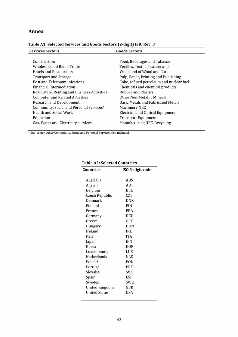
43
Annex Table A1: Selected Services and Goods Sectors (2digit) ISIC Rev. 3
Services Sectors Goods Sectors Construction Food, Beverages and Tabacco Wholesale and Retail Trade Textiles, Textile, Leather and Hotels and Restaurants Wood and of Wood and Cork Transport and Storage Pulp, Paper, Printing and Publishing Post and Telecommunications Coke, refined petroleum and nuclear fuel Financial Intermediation Chemicals and chemical products Real Estate, Renting and Business Activities Rubber and Plastics Computer and Related Activities Other Non‐Metallic Mineral Research and Development Basic Metals and Fabricated Metals Community, Social and Personal Services* Machinery NEC Health and Social Work Electrical and Optical Equipment Education Transport Equipment Gas, Water and Electricity services Manufacturing NEC, Recycling
* Sub‐sector Other Community, Social and Personal Services also included.
Table A2: Selected Countries
Countries ISO 3digit code Australia AUS Austria AUT Belgium BEL Czech Republic CZE Denmark DNK Finland FIN France FRA Germany DEU Greece GRC Hungary HUN Ireland IRL Italy ITA Japan JPN Korea KOR Luxembourg LUX Netherlands NLD Poland POL Portugal PRT Slovalia SVK Spain ESP Sweden SWE United Kingdom GBR United States USA

44
Table A3: Summary Statistics Country Attributes
Min. 10th 25th 50th 75th 90th Max Std. Dev. High‐skilled ln (H/L)o ‐2.5773 ‐1.9604 ‐1.7752 ‐1.5830 ‐1.2902 ‐1.0856 ‐0.8262 0.3525 Mid‐skilled ln (M/L)o ‐1.2344 ‐1.1716 ‐1.0754 ‐0.9267 ‐0.8266 ‐0.7760 ‐0.7042 0.1429 ICT capital ln (Kit/L)o ‐6.0298 0.0387 0.3598 0.9738 2.8740 5.1733 5.5547 2.3551 Rule of Law Rulawo 0.2791 0.6974 0.8552 1.4316 1.7503 1.8810 1.9747 0.4784 Trust Tursto ‐0.3021 ‐0.2671 ‐0.1321 .0254 0.2079 0.2829 0.2979 .1971 Government Efficiency Goveffo 0.3983 0.7409 0.9346 1.7178 1.9648 2.0986 2.3038 0.5456 Regulatory Quality Regqo 0.4544 0.7528 0.9788 1.3427 1.6559 1.8029 2.0113 0.4016
Table A4: Summary Statistics Pairwise Correlation Country Atributes
log (H / L)o log (M/L)o log (Kit/L)o Rulawo Tursto Goveffo Regqo ln (H/L)o 1.0000 ln (M/L)o ‐0.3185* 1.0000 ln (Kit/L)o ‐0.4060* 0.2012* 1.0000 Rulawo 0.5970* 0.1948* ‐0.2477* 1.0000 Tursto 0.6083* 0.2732* ‐0.0450* 0.9198* 1.0000 Goveffo 0.6477* 0.1895* ‐0.3427* 0.9560* 0.9239* 1.0000 Regqo 0.6870* 0.1053* ‐0.3695* 0.8770* 0.8021* 0.9008* 1.0000
Note: * denotes significance at the 1% level. Bonferroni adjusted significance level included.

45
Table A5: Summary Statistic Sector Characteristics (Services)
Min. 10th 25th 50th 75th 90th Max Std. Dev. High‐skilled ln (H/L)s ‐4,9654 ‐3,1252 ‐2,5610 ‐1,7952 ‐1,1611 ‐0,7485 ‐0,5105 0,9296 Mid‐skilled ln (M/L)s ‐3,0267 ‐1,1661 ‐0,7680 ‐0,4917 ‐0,3106 ‐0,1798 ‐0,0220 0,4443 ICT capital ln (Kit/L)s ‐7,8221 ‐1,4023 ‐0,0806 1,0223 2,7808 4,4808 8,4754 2,6890 Herfindahl Index HISs 0,0030 0,0315 0,0507 0,0828 0,1454 0,2316 0,8121 0,0951 Relationship specificity RS3s 0,0902 0,3847 0,5291 0,6897 0,7850 0,8639 0,9900 0,1878 Entry Barriers DER Entrys 0,0201 0,1536 0,2091 0,2996 0,4218 0,5255 0,7294 0,1418 Conduct Regulation DER Conds 0,0620 0,1815 0,2490 0,3417 0,4422 0,5462 0,8472 0,1453 FDI Restrictions DER FDIs 0,1232 0,3299 0,4183 0,5231 0,6394 0,7615 0,9232 0,1612
Table A6: Summary Statistics Pairwise Correlation Sector Characteristics (Services)
log (H/L)s log (M/L)s log (Kit/L)s HISs RS3s DER Entrys DER Conds DER FDIs ln (H/L) s 1.0000 ln (M/L) s ‐0.1927* 1.0000 ln (Kit/L)s 0.1298* 0.1321* 1.0000 HIS s 0.2440* ‐0.0193* 0.0809* 1.0000 RS3s 0.3537* ‐0.0349* 0.0441* 0.7863* 1.0000 DER Entrys 0.2003* 0.0334* 0.1461* 0.5931* 0.7566* 1.0000 DER Conds 0.3139* 0.0500* 0.0603* 0.6495* 0.8130* 0.8612* 1.0000 DER FDIs 0.2011* 0.0371* 0.0319* 0.7714* 0.9199* 0.8127* 0.8276* 1.0000
Note: * denotes significance at the 1% level. Bonferroni adjusted significance level included.

46
Table A7: Anticipated effects of EU membership
(1) (2) (3) Services Services Services OLS OLS OLS ln(Xodst) ln(Xodst) ln(Xodst) GEO ln (Distance) ‐0.600*** ‐0.565*** ‐0.521*** (0.118) (0.123) (0.131)
Contiguity 1.072*** 1.103*** 1.144*** (0.197) (0.200) (0.206)
Language ‐0.153 ‐0.168 ‐0.189 (0.264) (0.264) (0.265)
Colony ‐0.0710 ‐0.0555 ‐0.0349 (0.179) (0.181) (0.183)
Legal 0.652*** 0.659*** 0.671*** (0.192) (0.192) (0.193)
EU 2003 0.669* (0.391)
EU 2002 0.833** (0.419)
EU 2001 1.035** (0.463)
FE Exp‐year Yes Yes Yes FE Imp‐sector‐year Yes Yes Yes Observations 9353 9353 9353 R2 0.761 0.761 0.761
Notes: ***, ** and * denote significance at the 1%, 5% and 10% levels respectively. Robust standard errors with importer‐sector and exporter fixed effects for all specifications and clustered by country pair. All columns apply for services trade.

47
Table A8: Institutionally dependant variable by way of input use through deregulation of Entry Barriers (19992005)
Services Sectors DER Entrys
Financial Intermediation 0,47 Post and Telecommunications 0,46 Computer and Related Activities 0,41 Wholesale and Retail Trade 0,38 Transport and Storage 0,37 Real Estate, Renting and Business Activities 0,35 Research and Development 0,32 Education 0,30 Gas, Water and Electricity services 0,28 Community, Social and Personal Services* 0,27 Hotels and Restaurants 0,23 Health and Social Work 0,23 Construction 0,17
* Unweighted average of Community, Social and Personal Services and Other Community, Social and Personal Services.
Recommended