Defence R&D Canada
Centre for Operational Research and Analysis
Canadian Operational Support CommandOperational Research & Analysis
Design of Tactical Support Strategies in Military Logistics: Trade-offs Between Efficiency and EffectivenessA Column and Cut Generation Modeling Methods
S. Sebbah
NSERC Visiting Fellow, CANOSCOM Operational Research & Analysis
A. Ghanmi
CANOSCOM Operational Research & Analysis
A. Boukhtouta
CANOSCOM Operational Research & Analysis
DRDC CORA TM 2011-211December 2011


Design of Tactical Support Strategies in
Military Logistics: Trade-offs Between
Efficiency and EffectivenessA Column and Cut Generation Modeling and Solution Methods
S. Sebbah
NSERC Visiting Fellow, CANOSCOM Operational Research & Analysis
A. Ghanmi
CANOSCOM Operational Research & Analysis
A. Boukhtouta
CANOSCOM Operational Research & Analysis
Defence R&D Canada – CORA
Technical Memorandum
DRDC CORA TM 2011-211
December 2011

Principal Author
Original signed by S. Sebbah
S. Sebbah
Approved by
Original signed by P. Archambault
P. Archambault
Acting Section Head, Land Systems and Operations
Approved for release by
Original signed by P. Comeau
P. Comeau
Chief Scientist, DRDC CORA
c© Her Majesty the Queen in Right of Canada as represented by the Minister of
National Defence, 2011
c© Sa Majesté la Reine (en droit du Canada), telle que représentée par le ministre
de la Défense nationale, 2011

Abstract
Military tactical logistics planning is concerned with the problem of distributing
heterogeneous commodities (e.g., fuel, food, ammunition, etc.) from main operat-
ing bases to forward operating bases in a theatre of operations using a combination
of heterogeneous transportation assets such as logistics trucks and tactical heli-
copters. Minimizing the sustainment cost while satisfying the operational demand
under time and security constraints is of high importance for the Canadian Forces.
In this study, a logistics planning model is developed to explore effective and ef-
ficient strategies for tactical logistics distribution. A mathematical optimization
algorithm based on a column and cut generation technique, using Gomory-Chvátal
rank−1 cuts, is developed to solve the problem.
This report presents details of a mathematical formulation and a solution algorithm
along with an example application to demonstrate the methodology. Computational
results are presented in order to measure the degree of efficiency and scalability
of the proposed approach, and to study the trade-off between the efficiency and
effectiveness in the resulting sustainment strategies.
Résumé
Le problème propre à la planification de la logistique tactique militaire concerne
la distribution de biens hétèrogènes (p. ex., du carburant, de la nourriture, des mu-
nitions, etc.) depuis des bases d’opérations principales vers des bases d’opérations
avancées dans un théâtre d’opérations, à l’aide de moyens de transport hétérogènes
tels que des camions et des hélicoptères tactiques. Il est primordial pour les Forces
canadiennes de réduire au minimum le coût du maintien en puissance, tout en ré-
pondant aux exigences opérationnelles malgré les contraintes qu’imposent le temps
et la sécurité. Dans la présente étude, un modèle de planification logistique est mis
au point pour explorer des stratégies efficientes et efficaces de distribution par les
services de logistique tactiques. Un algorithme d’optimisation mathématique fondé
sur le modèle de génération de colonnes et de coupes et utilisant les plans de coupe
d’ordre 1 de Gomory-Chvàtal est élaboré pour régler le problème.
DRDC CORA TM 2011-211 i

This page intentionally left blank.
ii DRDC CORA TM 2011-211

Executive summary
Design of Tactical Support Strategies in Military
Logistics: Trade-offs Between Efficiency and
Effectiveness
S. Sebbah, A. Ghanmi, A. Boukhtouta; DRDC CORA TM 2011-211;
Defence R&D Canada – CORA; December 2011.
Background: Military tactical logistics planning is concerned with the problem of
distributing heterogeneous commodities (e.g., fuel, food, ammunition, etc.) from
Main Operating Bases (MOBs) to Forward Operating Bases (FOBs) in a theatre
of operations using a combination of heterogeneous transportation assets such as
logistics trucks and tactical helicopters. Given the amount of supplies the Canadian
Forces (CF) transports during each mission, optimization of the sustainment costs
is becoming a primordial issue in order to effectively and efficiently continue to
support the CF deployed troops.
In the design of supply chain strategies, decision-makers are facing the challenge
of finding good trade-offs between efficiency and effectiveness, which are related
to the cost of achieving an objective and the degree of satisfaction of that objective.
The CF is continually making tactical decisions to strike good trade-offs between
efficiency and effectiveness during deployment and sustainment phases. In this
study, we focus on the design of tactical logistics strategies, which achieve different
optimal balances between support efficiency and its effectiveness, i.e., meet the re-
quirements of the troops with the optimal supply cost. We introduce a new concept
"Quality-of-Support (QoS)" which is a combination of parameters that measure the
effectiveness of the elaborated support strategies. These parameters are the lead-
time, safety of routes, security in transportation of commodities, and reliability of
transportation assets.
Objective and scope: The objective of this research is to develop a scalable and ef-
ficient mathematical optimization method to the military tactical logistics planning
problem. Our main goal is to provide the military decision makers with a practical
tactical logistics planning tool that will help in striking good trade-offs between
efficiency and effectiveness in elaborating tactical support strategies. In this work,
we tried to answer the question: if you are given a tactical logistics network, a set of
heterogeneous transportation assets of different classes and modes (land, air) with
different capacities, speed, range, etc., a set of heterogeneous commodities, a set of
end-users requesting different commodities with different QoS requirements, then,
what is the optimal way, in terms of cost, to load and route an optimal fleet-size
DRDC CORA TM 2011-211 iii

(to be determined) of transportation assets to carry the different commodities with
their associated QoS requirements to their destinations?
Significance of contributions and results: In this study, a tactical logistics plan-
ning method, that is to be integrated into a logistics decision support system, is
developed. We analyzed the trade-offs between cost, lead-time and safety of routes
with different demand patterns of commodities. The obtained results can be used
to estimate a weekly sustainment cost given the targeted QoS. Furthermore, for
different distributions of demands over a given lead-time interval, we showed the
distribution of the number of lifts over the classes of transportation assets. These
statistics would be used to compose the optimal support fleet to respond to the ter-
rain reality and the challenge of meeting the requirement of different demands. The
analysis of the safety of land routes showed that this parameter has a significant
impact on the support cost. Different levels of safety of routes were considered and
the inherent cost was analyzed. The computational results obtained in this study
and the proposed algorithmic approach are recommended in "what-if" tactical lo-
gistics analyses and design of large scale tactical logistics strategies, respectively.
Different perspectives were explored and several alternatives were analyzed to help
decision makers to strike different balances between efficiency and effectiveness in
tactical support and to respond efficiently to different situations.
Future work: While the main focus of this work is on military sustainment strate-
gies to achieve optimal trade-offs between efficiency and effectiveness, further im-
provement and extension of the methodology could be considered. First and fore-
most, the problem of the convoy formation and escorting, and how it affects the se-
lection of transportation assets and their routing. The convoy escorting cost, which
is part of the operational cost, is not considered in this study. Including this pa-
rameter in the study will probably change the modeling and solution approach and
the optimal solution. Secondly, we assume different percentages of reliability of
randomly selected land routes. However, if all land routes are unsafe and a limited
escorting budget has to be met, then, a question arises which routes to secure in
order to optimize the support cost? Or, how to form and route the convoys given
the safety status of the routes?
Some other questions are still open: how similar or different are the two problems of
optimizing the tactical logistics footprint (number of transportation assets) and the
problem of optimizing the operational cost? Or, does optimization of the footprint
implies the operational cost (and vice versa)? The answer is not straightforward and
necessitates more investigation. In this study, we focused on the impact of safety of
routes on the support cost, however, other facilities may fail as well as routes (e.g.,
MOBs, Depots). This research direction is highly promising, and our proposal
iv DRDC CORA TM 2011-211

of tactical logistics design strategies could be extended to survive intentional and
accidental disruptions by building back-up strategies.
DRDC CORA TM 2011-211 v

Sommaire
Design of Tactical Support Strategies in Military
Logistics: Trade-offs Between Efficiency and
Effectiveness
S. Sebbah, A. Ghanmi, A. Boukhtouta ; DRDC CORA TM 2011-211 ;
R & D pour la défense Canada – CARO ; décembre 2011.
Contexte : Le problème propre à la planification de la logistique tactique militaire
concerne la distribution de biens hétérogènes (p. ex., du carburant, de la nourriture,
des munitions, etc.) depuis des bases d’opérations principales (BOP) vers des bases
d’opérations avancées (BOA) dans un théâtre d’opérations, à l’aide de moyens de
transport hétérogènes tels que des camions et des hélicoptères tactiques. Vu la quan-
tité d’approvisionnements que les FC transportent au cours de chaque mission, l’op-
timisation du maintien en puissance devient un objectif primordial pour que les
Forces canadiennes puissent continuer de soutenir avec efficacité et efficience leurs
troupes en déploiement. Quand les décideurs conçoivent des stratégies relatives à
la chaîne d’approvisionnement, ils doivent trouver de bons compromis entre l’effi-
cience et l’efficacité, compromis qui se rapportent au coût à subir pour atteindre un
objectif et à la mesure dans laquelle ce dernier sera effectivement réalisé. Les FC
prennent constamment des décisions tactiques pour en arriver à de bons compromis
entre l’efficience et l’efficacité aux stades du déploiement et du maintien en puis-
sance. Dans la présente étude, nous nous concentrons sur l’élaboration de stratégies
de logistique tactique qui aboutissent à divers équilibres optimums entre l’efficience
et l’efficacité du soutien (satisfaire aux besoins des troupes, tout en maintenant le
coût du ravitaillement à un niveau optimal). Nous présentons un nouveau concept,
soit celui de la "Qualité du Soutien" (QdS), qui résulte d’une combinaison de pa-
ramètres utilisés pour mesurer l’efficacité des stratégies de soutien élaborées. Ces
paramètres sont les suivants : le délai d’exécution, la sécurité des itinéraires et du
transport des biens, et la fiabilité des moyens de transport.
Objectif et portée : La présente étude vise à élaborer une méthode d’optimisation
mathématique extensible et efficiente pour régler le problème posé par la planifica-
tion de la logistique tactique militaire. Notre principal objectif consiste à procurer
aux décideurs militaires un outil de planification pratique qui, en matière de logis-
tique tactique, les aidera à trouver de bons compromis entre l’efficience et l’effi-
cacité quand ils élaboreront leurs stratégies de soutien tactique. Nous avons tenté
ici de répondre à la question suivante : étant donné un réseau logistique tactique,
un ensemble de ressources de transport hétérogènes appartenant à diverses classes
et modes (terre, air) et ayant différentes capacités, vitesses et autonomies, etc., une
vi DRDC CORA TM 2011-211

gamme de biens hétérogènes (besoins exprimés) et des utilisateurs finaux qui de-
mandent différents biens et dont les besoins en matière de QdS varient, quelle est la
façon optimale, quant au coût, de charger les différents biens à bord d’une flotte de
taille optimale (à définir) pour qu’elle les transporte, en suivant l’itinéraire choisi,
jusqu’à leurs destinations tout en répondant aux besoins connexes relatifs à la QdS ?
Importance des contributions et des résultats : Dans la présente étude, nous
élaborons une méthode de planification de la logistique tactique qui doit être in-
tégrée dans un système de soutien du processus décisionnel relatif à la logistique.
Dans l’analyse, nous opérons des compromis entre le coût, le délai d’exécution et
la sécurité des itinéraires dans le cadre de différentes répartitions des besoins. Les
résultats obtenus pourraient servir à estimer le coût hebdomadaire du maintien en
puissance, compte tenu de la QdS voulue. En outre, pour différentes répartitions
des besoins au cours d’un délai d’exécution donné, nous avons montré la réparti-
tion du nombre de voyages entre les catégories de moyens de transport. Ces sta-
tistiques serviront ensuite à composer la flotte de soutien optimale en fonction des
caractéristiques réelles du terrain et du défi consistant à répondre aux besoins des
différents utilisateurs. L’analyse de la sécurité des routes terrestres a montré que
ce paramètre influe considérablement sur le coût du soutien. Nous avons examiné
différents degrés de danger sur les routes et nous avons analysé le coût inhérent
des déplacements sur ces dernières. Les résultats computationnels obtenus au cours
de l’étude et la démarche algorithmique proposée sont recommandés dans des ana-
lyses hypothétiques sur la logistique tactique et dans la conception de stratégies de
grande envergure en matière de logistique tactique, respectivement. Nous avons en-
visagé diverses perspectives et analysé plusieurs solutions de rechange pour aider
les décideurs à trouver différents équilibres entre l’efficience et l’efficacité dans le
soutien tactique et à faire face avec efficience à différentes situations.
Travail à venir : Notre étude porte principalement sur les stratégies militaires de
maintien en puissance devant permettre d’opérer des compromis optimums entre
l’efficience et l’efficacité, mais on pourrait envisager d’améliorer la méthodologie
et d’en étendre encore plus la portée. Tout d’abord, songeons au problème de la for-
mation et de l’escorte des convois et à la façon dont il influe sur le choix des moyens
de transport et des itinéraires. Dans la présente étude, nous ne prenons pas en consi-
dération le coût de l’escorte des convois, qui fait partie du coût opérationnel. Si l’on
inclut ce paramètre dans l’étude, cela changera sans doute l’approche de la modé-
lisation et de la définition de la solution ainsi que la solution optimale. En second
lieu, nous supposons différents pourcentages de fiabilité à l’égard d’itinéraires ter-
restres choisis au hasard. Cependant, si tous les itinéraires terrestres sont dangereux
et qu’il faut s’en tenir à un budget limité pour l’escorte, la question se pose de sa-
voir quels itinéraires il faut sécuriser pour optimiser le coût du soutien. Ou encore,
comment former et diriger les convois, étant donné le degré de sécurité de ces iti-
DRDC CORA TM 2011-211 vii
néraires ? D’autres questions sont encore en suspens : dans quelle mesure les deux
problèmes qui consistent à optimiser les ressources de transport affectées à la logis-
tique tactique, d’une part, et, d’autre part, le coût opérationnel sont-ils semblables,
ou différents ? Ou encore, l’optimisation des ressources va-t-elle de pair avec le coût
opérationnel (et vice versa) ? La réponse n’est pas évidente et elle nécessite d’autres
recherches. Dans la présente étude, nous avons mis l’accent sur l’effet de la sécurité
des itinéraires sur le coût du soutien. Cependant, hormis les itinéraires, d’autres élé-
ments infrastructurels (p. ex., les BOP, les dépôts) peuvent flancher. L’orientation
que notre recherche offre est très prometteuse, et notre proposition d’élaborer des
stratégies de logistique tactique pourrait être élargie, de manière que l’on en vienne
à dresser des stratégies auxiliaires pour survivre à des bouleversements intention-
nels ou accidentels.
viii DRDC CORA TM 2011-211

Table of contents
Abstract . . . . . . . . . . . . . . . . . . . . . . . . . . . . . . . . . . . . . i
Résumé . . . . . . . . . . . . . . . . . . . . . . . . . . . . . . . . . . . . . i
Executive summary . . . . . . . . . . . . . . . . . . . . . . . . . . . . . . . iii
Sommaire . . . . . . . . . . . . . . . . . . . . . . . . . . . . . . . . . . . . vi
Table of contents . . . . . . . . . . . . . . . . . . . . . . . . . . . . . . . . ix
List of figures . . . . . . . . . . . . . . . . . . . . . . . . . . . . . . . . . . xi
Acknowledgements . . . . . . . . . . . . . . . . . . . . . . . . . . . . . . . xii
1 Introduction . . . . . . . . . . . . . . . . . . . . . . . . . . . . . . . . . 1
1.1 Preliminaries . . . . . . . . . . . . . . . . . . . . . . . . . . . . . 1
1.2 Analysis of the problem and literature review . . . . . . . . . . . . 2
1.3 Objective and scope . . . . . . . . . . . . . . . . . . . . . . . . . 5
1.4 Organization . . . . . . . . . . . . . . . . . . . . . . . . . . . . . 7
2 Tactical support network model . . . . . . . . . . . . . . . . . . . . . . . 8
2.1 Support efficiency . . . . . . . . . . . . . . . . . . . . . . . . . . 12
2.2 Support effectiveness . . . . . . . . . . . . . . . . . . . . . . . . 12
3 Mathematical modeling and solution methods . . . . . . . . . . . . . . . 14
3.1 Column generation decomposition based on support plans . . . . . 15
3.2 Master model . . . . . . . . . . . . . . . . . . . . . . . . . . . . 17
3.3 Pricing model . . . . . . . . . . . . . . . . . . . . . . . . . . . . 18
3.4 Lead-time constraints . . . . . . . . . . . . . . . . . . . . . . . . 21
3.5 Support reliability constraints . . . . . . . . . . . . . . . . . . . . 23
3.5.1 Security and suitability of transportation assets . . . . . . 23
3.5.2 Commodities clustering . . . . . . . . . . . . . . . . . . 23
DRDC CORA TM 2011-211 ix

3.5.3 Safety of routes . . . . . . . . . . . . . . . . . . . . . . . 24
3.6 Gomory-Chvátal rank-1 cutting planes . . . . . . . . . . . . . . . 24
3.7 Solution algorithm . . . . . . . . . . . . . . . . . . . . . . . . . . 26
4 Computational results . . . . . . . . . . . . . . . . . . . . . . . . . . . . 28
4.1 The tactical support model . . . . . . . . . . . . . . . . . . . . . . 28
4.2 The benchmark data inputs . . . . . . . . . . . . . . . . . . . . . 29
4.3 Performance assessment . . . . . . . . . . . . . . . . . . . . . . . 30
4.4 Trade-off between lead-time and cost . . . . . . . . . . . . . . . . 32
4.5 Trade-off between lead-time and types of lifts . . . . . . . . . . . 34
4.6 Trade-off between safety of routes and cost . . . . . . . . . . . . . 39
5 Conclusions and future work . . . . . . . . . . . . . . . . . . . . . . . . 41
5.1 Summary of principal results . . . . . . . . . . . . . . . . . . . . 41
5.2 Future work . . . . . . . . . . . . . . . . . . . . . . . . . . . . . 42
References . . . . . . . . . . . . . . . . . . . . . . . . . . . . . . . . . . . . 43
List of Acronyms . . . . . . . . . . . . . . . . . . . . . . . . . . . . . . . . 47
Annex A: Price and cut models . . . . . . . . . . . . . . . . . . . . . . . . 49
Annex B: Further computational results . . . . . . . . . . . . . . . . . . . . 53
x DRDC CORA TM 2011-211

List of figures
Figure 1: Generic JTFSC Joint Task Force . . . . . . . . . . . . . . . . . . 8
Figure 2: JTFSC schematic theatre lay-out . . . . . . . . . . . . . . . . . . 9
Figure 3: Different JTFSC configurations . . . . . . . . . . . . . . . . . . 11
Figure 4: A support plan . . . . . . . . . . . . . . . . . . . . . . . . . . . 16
Figure 5: Computation approach of lead-time . . . . . . . . . . . . . . . . 23
Figure 6: ILP and cuts . . . . . . . . . . . . . . . . . . . . . . . . . . . . 25
Figure 7: The solution algorithm . . . . . . . . . . . . . . . . . . . . . . . 27
Figure 8: Trade-off between cost and lead-time . . . . . . . . . . . . . . . 33
Figure 9: Number of lifts vs. constrained lead-time ≤ TSP . . . . . . . . . 35
Figure 10: Number of lifts vs. constrained lead-time ≤ 1.5∗TSP . . . . . . . 36
Figure 11: Number of lifts vs. constrained lead-time ≤ 2∗TSP . . . . . . . . 36
Figure 12: Number of lifts vs. constrained lead-time ≤ 2.5∗TSP . . . . . . . 37
Figure 13: Number of lifts vs. constrained lead-time ≤ 2.6∗TSP . . . . . . . 37
Figure 14: Number of lifts vs. constrained lead-time ≤ 2.8∗TSP . . . . . . . 38
Figure 15: Trade-off between cost and safety of land routes . . . . . . . . . 40
DRDC CORA TM 2011-211 xi

Acknowledgements
The author would like to thank LCol T. Gibbons, Maj J. Lycon and Maj K. Chow
for their valuable comments and suggestions on the tactical support model.
xii DRDC CORA TM 2011-211

1 Introduction
1.1 Preliminaries
Military tactical logistics planning addresses the problem of distributing heteroge-
neous commodities (e.g., fuel, food, ammunition, etc.) from Main Operating Bases
(MOBs) to Forward Operating Bases (FOBs) in a theatre of operations using a com-
bination of heterogeneous transportation assets such as logistics trucks and tactical
helicopters. The Canadian Forces (CF) makes extensive use of a variety of tac-
tical transportation assets to supply its oversea deployments, and sometimes uses
multiple sources of supply.
Given the amount of supplies the CF transports during each mission, optimization
of the sustainment costs is becoming crucial to the effective and efficient support
of CF deployed troops. In the design of supply chain distribution strategies, partic-
ularly in the military, there are different trade-offs between the capital/operational
cost and the achievable supply performance [1–3]. In this report, we use these two
metrics to measure the efficiency and the effectiveness of military support strate-
gies, respectively. These trade-offs are key to developing the most efficient and
effective logistics and supply chain management strategy. Focusing solely on the
supply cost may results in strategies that are less flexible and not effective in meet-
ing the requirements of deployed troops. For example, using a land transportation
mode, e.g., trucks, to reduce transportation costs may increase the delivery time and
the vulnerability of the transported supplies. Furthermore, a flexible supply strategy
is the one that can be dynamically changed to respond to a new unexpected event
with less disturbance of the whole supply chain. Such a supply strategy is usually
not necessarily highly optimized [4–7].
In the design of supply chain strategies, decision-makers face the challenge of find-
ing good trade-offs between efficiency and effectiveness, which are related to the
cost of achieving an objective and the degree of satisfaction reached toward that ob-
jective. In the military, the trade-off between efficiency and effectiveness appears at
different levels during the deployment and sustainment phases of operations. Dur-
ing the deployment phase, the operational support goals are to ensure deployment
speed by reducing the time as much as possible while keeping its cost at its low-
est value. Similarly, during the sustainment phase, the objective is to ensure that
the deployed forces are able to achieve their objectives during this period while
minimizing the cost to provide the required support level. Therefore, in the design
of military supply strategies, the focus should be on cost-efficient strategies that
guarantee some Quality-of-Supply (QoS) parameters (e.g., sustainment lead-time,
security, integrity, etc.).
Organizations struggle to achieve efficiency and effectiveness. The CF, because
DRDC CORA TM 2011-211 1

of its size and complexity, is continually called to elaborate strategies and take
decisions at different levels to balance between these two dual concepts. In terms of
logistics, although integrating QoS considerations in the design of supply strategies
may increase the supply cost, their advantages in some cases largely offset their
costs. The scientific literature on the trade-off between efficiency and effectiveness
with real-world characteristics in logistics planning is not rich. Some references
[3, 4, 8, 9] provided qualitative studies and comparative analysis of the trade-off
between the two concepts.
Several inter-related problems need to be addressed in the design of military logis-
tics networks. The design problem includes strategic decisions, such as the location
of the main and forward operating bases, forward support groups, communication
technology, and transportation modes. Once the logistics network physical configu-
ration is determined, the focus shifts to the tactical and operational level’s decisions,
such as distribution decisions of supplies within the network. Several studies have
considered the location and distribution issues in the design of industrial logistics
networks [10] and some in military strategic logistics [11–13].
In this study, we focus on the design of tactical logistics strategies, which achieve
different optimal balances between supply efficiency and its effectiveness, i.e., meet
the QoS requirements of the troops with the optimal supply cost. From the opti-
mization point of view, our main concern is to find the optimal loading and routing
of an optimized fleet-size of heterogeneous transportation assets, given transporta-
tion capacity and security constraints, to supply the different FOBs while meeting
the expressed QoS in terms of supply lead-time and security.
1.2 Analysis of the problem and literature review
Our tactical logistics planning problem can be divided into two sub-problems: load-
ing of commodities onto transportation assets and routing of the loaded transporta-
tion assets. These two problems are solved jointly to identify the optimal fleet mix
of transportation assets to meet the demands of the end-users with the required
QoS. For the loading of commodities sub-problem, in addition to the classical con-
straints inherent to the capacity (payload and bulk capacities) of the transportation
assets, there are some additional constraints related to security issues (e.g., ammu-
nition is transported separately) and reliability of transportation assets (e.g., some
truck classes are more suitable, due to their reliability, to transport some classes
of commodities than others). These constraints cannot be treated separately as they
directly affect the loading of commodities and the selection of the appropriate trans-
portation assets. The routing sub-problem involves finding the optimal routing of
an optimal fleet mix of transportation assets to provide QoS guarantees to the dif-
ferent FOBs. In planning of the transportation assets routing, constraints inherent
2 DRDC CORA TM 2011-211

to the range of the used transportation assets, their cruising speed, and reliability
should be taken into consideration in the selection of the routing plan. Planning of
these two sub-problems cannot be done separately as they are related to each other,
and their constraints overlap.
Our loading and routing sub-problems are closely related to the Multi-Bin Pack-
ing Problem (MBPP) [14] and the Capacitated Vehicle Routing Problem with Time
Window (CVRPTW) [15], respectively. The MBPP requires the determination of
a packing pattern of a given set of items into a minimum number of identical or
different bins. While in the CVRPTW, the objective is to determine the optimal
routing of a fleet of capacitated vehicles in order to supply clients who have time
windows within which the deliveries must be made. By analogy, our loading prob-
lem involves loading of standard units of commodities (pallets) of different weights
onto trucks and helicopters of different payload and bulk capacities. Furthermore,
incompatibility constraints between goods and between goods and transportation
classes are added in our case. The commodities-clustering constraints state that
some classes of commodities are not mixed with others, and the reliability of trans-
portation assets forbids the loading of some classes of commodities on some classes
of transportation assets. In our tactical logistics problem, the transportation model
involves routing of trucks and helicopters of different capacities to serve FOBs with
time windows (lead time) supporting a split-delivery strategy. Indeed, as most of the
demands cannot be loaded onto a single transportation asset, several trucks and/or
helicopters would be needed to satisfy the demands of any FOB.
It is clear that our problem is N P−Hard 1 since it generalizes the CVPR and the
BPP. Different solutions to handle the loading and routing of transportation assets
have been proposed to solve several logistics problems where the objective was to
optimize the operational cost and meet different loading and routing constraints.
In [15], Laporte presented an exhaustive review of the several extensions proposed
for the VRP, and a classification of the different extensions was made according to
some characteristics: (i) topology: demand locations to be satisfied, their number,
number of depots, etc.; (ii) vehicles: homogeneous/heterogeneous fleet, fixed or
variable fleet size, similar or different capacities, time windows for vehicle avail-
ability; (iii) supply strategy: split delivery, mixed delivery, time windows; (iv)
objective: minimize the supply footprint, penalties in case where the service re-
quirements are not met, penalties implying fleet size. Most of the vehicle routing
problems are at least N P -hard. A variety of solutions based on heuristics, and exact
methods have been developed to the different versions of the problem [15–19].
Some previous studies of the VRP have considered different versions of the vehicles
1. Non-deterministic polynomial-time hard. The optimization problem, "what is the optimal
solution of the loading and routing problem in our tactical logistics problem?", is NP-hard, since
there is no easy way (polynomial-time algorithm) to determine if a solution is the optimal one.
DRDC CORA TM 2011-211 3

loading problem. In [20], Rebeiro and Soumis treated vehicles as commodities. In
their non-split VRP model, trips are pre-determined and the problem is to allocate
one vehicle to each trip. The authors proposed a Column Generation (CG) solu-
tion method, and showed that the optimal Linear Problem (LP) relaxation gives a
good bound for the Integer Linear Problem (ILP). In [21], Fisher et al. also treated
vehicles as commodities. The authors proposed a mixed-delivery VRP where each
vehicle is restricted to carry one order at a time. Approximation algorithms have
been proposed to effectively approach feasible good solutions. In [22], Malapert
et al. proposed a constrained programming based approach to the two-dimensional
pickup and delivery routing problem with loading constraints. Therein, the set of
items requested by each client can be loaded onto a single vehicle, though split
deliveries are not allowed. The objective was to find a partition of the clients into
routes of a minimal total cost, such that for each route there exists a feasible loading
of the items onto the vehicle loading surface that satisfies the capacity constraints.
In [23], Iori et al. proposed an exact approach based on branch-and-cut for the vehi-
cle routing problem with two-dimensional loading constraints. The considered case
is a symmetric capacitated vehicle routing problem in which a fleet of K identical
vehicles are used to serve customers. All vehicles are identical and have a known
lift capacity and a single rectangular loading surface. All items of a given customer
must be assigned to a single vehicle (called item clustering constraints). Further-
more, sequential loading constraints are added: items of a customer must not be
blocked by items of customers to be visited later along the route.
The vehicle fleet mix optimization problem has been studied by some scientists
at the Defence Research and Development Canada (DRDC). Kaluzny and Erke-
lens [24], in support of the project office management Medium Support Vehicle
System (MSVS), studied the optimal mix of MSVS required for the replenishment
of first line units. The study computed the minimum number of vehicles needed to
transport the lift requirements using an optimization approach based on a classical
ILP approach. Different configurations of transportation trucks with different trans-
portation capabilities were considered and recommendations of a fleet of vehicles
that minimizes the logistics footprint (number of trucks) of deployed combat service
support units were formulated. Asiedu [25] has extended the work and presented a
study to assess the impact of using 8-tonne variants of trucks on the optimal vehicle
fleet mix. Asiedu and Hill [26] have proposed a new approach to tactical logistics
support fleet mix planning, which includes some dynamic aspects of the logistics
problem. The authors proposed an integrated simulation and classical ILP-based
optimization method to optimize the vehicle fleet mix given a set of dynamic op-
erational factors. Given a number of vehicles and containers, the proposed method
selects the optimal fleet mix that optimizes a multi-term objective function.
Although the tactical logistics planning problem considered in this study involves
vehicle routing and loading, it is quite different from the classical CVRPTW with
4 DRDC CORA TM 2011-211

loading constraints. Indeed, we have: (i) heterogeneous transportation assets of
two modes (land, air) with different characteristics, i.e., capacity, speed, range, op-
erational cost, reliability, which can transport different classes of commodities but
not all; (ii) multiple classes of commodities with different weights which could
be transported on some classes of transportation assets but not necessarily on oth-
ers depending on the reliability of the transportation asset and the sensitivity of
the transported commodity; (iii) demands for commodities are expressed with QoS
parameters including time and reliability, although, for each destination and com-
modity, there are transportation and loading constraints to be observed; (iv) de-
pending on the range of the transportation assets and the traveled distance, multiple
transportation assets of different classes would be necessary to convey a given com-
modity to its destination. This configuration also happens when different lead-times
have to be met; (v) the objective is to minimize an objective function of the operat-
ing cost, and at the same time meet the lead-time of the different FOBs, and guar-
antee reliable delivery of the commodities. Based on these new practical aspects of
the problem, the routing and loading problems have to be re-designed in order to
meet the different new requirements. To the best of our knowledge this problem has
not been dealt with in the literature, and this study is the first to include the different
new practical aspects of the problem.
1.3 Objective and scope
The objective of this research is to develop a scalable and efficient mathematical op-
timization method to the military tactical logistics planning problem. Our main goal
is to provide the military decision makers with a practical tactical logistics planning
tool that will help in striking good trade-offs between efficiency and effectiveness
in elaborating tactical support strategies. This study tries to answer this question:
Given a tactical logistics network, a set of heterogeneous transportation assets of
different classes and modes (land, air) with different capacities, speed, range, etc.,
a set of heterogeneous commodities, a set of end-users requesting different com-
modities with different QoS requirements, then, what is the optimal way, in terms
of cost, to load and route an optimal fleet-size (to be determined) of transportation
assets to carry the different commodities with their associated QoS requirements to
their destinations?
This work is a major extension and enhancement over existing work in the literature.
The following characteristics of the military tactical support model, constraints, and
characteristics of the solution method are considered:
• Characteristics of the military tactical support model:
– two modes of transportation including air and land, and heterogeneous trans-
portation assets of different classes;
DRDC CORA TM 2011-211 5

– heterogenous commodities of different classes;
– demands for commodities are associated with QoS parameters;
– each land route is characterized by a binary safety status (safe, not safe);
– each pair of transportation class and land route is characterized by a binary
status (practicable or not) stating whether transportation assets of the class can
travel on the specified land route.
– similarly, each pair of transportation class and class of commodity is charac-
terized by a binary status (can be transported or not) stating whether trans-
portation assets of the class can transport commodities of the specified class.
– furthermore, each pair of two classes of commodities is characterized by a
binary status (can be clustered or not) stating whether commodities of the two
classes can be clustered on the same transportation asset.
– demands of any destination cannot be conveyed using a single lift.
• constraints in the military tactical support model:
– lead-time: demands for commodities issued at FOBs are required within dif-
ferent lead-times. Priorities are often associated with demands of commodities
in military logistics. The lead-time of demands decreases as their priorities in-
crease.
– reliability of transportation assets and transportation safety: transportation as-
sets of different classes have different levels of reliability, which could forbid
some loading patterns, e.g., loading of ammunition on light support trucks.
Furthermore, some commodities-clustering patterns are forbidden, because of
safety reasons during transportation. For example, ammunition is never clus-
tered with other commodities of other classes.
– land routes safety: land routes are not necessarily safe. In this case, in order to
ensure safe delivery of supplies, land routes known to be not safe are not used.
Furthermore, depending on the nature of the terrain e.g., stony routes, some
land route may be forbidden for some transportation assets of some specific
classes.
• The main characteristics of the proposed methodology and solution method are
summarized as follows:
– mathematical decomposition method based on CG is developed to obtain an
optimal solution to the Linear Problem (LP);
– the CG approach is augmented with a cut generation strategy, based on Gomory-
Chvátal rank−1 cuts, to cut off continuous solutions and strengthen the linear
bound in the derivation process of the integer solutions;
– three versions of the pricing model are developed to generate different trans-
portation strategies in order to meet the requirements in terms of lead-time and
safety;
– a column and cut generation algorithm is developed to use the different pieces
of the optimization models.
– the optimization model is a generic one, and can have as input different other
6 DRDC CORA TM 2011-211

classes of transportation assets and classes of commodities.
– the optimal combinations of trucks and helicopters are found for several values
of lead-time and different demand patterns.
This study focuses on cost efficient support strategies that are effective in achieving
a set of parameters. The main parameters we address regarding the support ef-
fectiveness are the on-time delivery of supplies, reliability of transportation assets,
security in transportation of commodities, and safety of routes.
1.4 Organization
This report is organized as follows. Section 2 gives an overview of our tactical
logistics network model. Section 3 provides mathematical optimization models and
solution algorithms for the considered problem. Section 4 presents the experimental
results and discusses the trade-off between efficiency and effectiveness. Section 5
concludes the report. Annex A contains the detailed Mixed Integer Linear Problems
(MILP), and Annex B contains the computational measuring of the performance of
the optimization algorithm.
DRDC CORA TM 2011-211 7

2 Tactical support network model
Canadian Operational Support Command (CANOSCOM) has recently proposed
a global military doctrine to provide enhanced operational support capability to a
Joint Task Force (JTF). The Joint Task Force Support Component Concept (JTFSC)
is defined as ". . . an integrated operational support formation of health services sup-
port, general support engineering, communication & information systems support,
military police, personnel support, logistics and land equipment maintenance units
and elements . . ." [27]. The JTFSC gathers all operational support elements de-
ployed with a JTF under a single JTFSC command. The JTFSC focus is general
support to JTF. It comprises a small JTFSC command and control element along
with a broad range of operational support functional capabilities. The component
structure within which the JTFSC functions is depicted in Figure 1 [27].
Figure 1: Generic JTFSC Joint Task Force
Based on the JTFSC schematic lay-out given in [27], we elaborated a more de-
tailed logistics support network (Figure 2) illustrating the JTFSC support compo-
nents, supported forces, and the flow of supplies. In a theatre of operations, the
JTFSC main component is located near the Sea or Air Port Of Disembarkation
((S/A)SPOD), and the detachment and forward components are located at the entry
point of the air forces and maritime forces, and at the MOBs and FOBs of the land
forces. These components serve as the in-theatre delivery formation that enhances
and sustains the JTF combat components.
In terms of supply flows, the JTFSC receives materiel and forces deploying at the
in-theatre APOD and SPOD and delivers these forward to FOBs to meet tactical
8 DRDC CORA TM 2011-211

requirements. In addition to the APOD and SPOD, operations could also be ex-
ternally supported by local sources (e.g., contractors), or established operational
support hubs. In Figure 2, the JTFSC support components are interconnected by
arrows, which define the supply network topology, showing the directions of the
supply flows. Two supply network topologies, overlapping on some arrows, are
shown to distinguish between land and air routes. These routes are established
based on the range of the trucks and helicopters used in transportation. If any of the
Figure 2: JTFSC schematic theatre lay-out
transportation assets, a truck or helicopter, can reach a point B from point A, then
a corresponding route (air or land) is added to illustrate that in the related supply
network topology. The arrows in the supply network topology give the reach-ability
of the different network components using the different transportation assets.
DRDC CORA TM 2011-211 9

The lower part of Figure 2 shows different classes of commodities, trucks, and he-
licopters. Each commodity class is associated with a weight per pallet, and each
truck and helicopter class is associated with a payload (Pc) and bulk (Bc) capac-
ity. The arrows departing from the commodities to the transportation assets show
some potential transportation relationships. In our supply model, depending on
the classes of the commodities (perishable, security sensitive, ammunition, etc.) a
transportation asset of a given class could be used because of its adaptability (e.g.,
safety and reliability), but others may not be used. In addition, because of the dan-
ger of mixing some classes of supplies, some commodities are never transported
together. What is not illustrated in the supply network topology of Figure 2 is the
potential allocations of transportation assets to routes. The illustrated arrows are
added whenever the range of any given class of transportation assets is greater or
equal to the distance of the route separating the two end-locations.
Figure 3 illustrates three more potential configurations of the JTFSC within differ-
ent theatres: (a) Two independent JTFSCs provide support to two deployed JTFs;
(b) a single JTFSC provides support to two deployed JTFs where supply does go
through a theatre to another; (c) a single JTFSC provides support to two deployed
JTFs where supply goes through one theatre to another (inter-theatre supply). These
configurations are potential JTFSC deployments. The main JTFSC coordinates its
efforts with its forward and detachment JTFSCs in the the tactical support at the
different locations to transport commodities to their destinations along the most
efficient ways.
10 DRDC CORA TM 2011-211

MOB
FOB
Units
FOBFOBUnits
TFSC
Units
Thea t re 2
Air
M a r i t i m e
MOB
FOB
Units
FOBFOBUnits
TFSC
Units
Thea t re 1
Air
M a r i t i m e
(a) Different JTFSC to supply different MOBs in different theatres
MOBFOB
Units
FOBFOBUnits
MOB
FOB
Units
FOB
Units
FOBUnits
TFSC
Units
Thea t re 1 Thea t re 2
Air
M a r i t i m e
Air
M a r i t i m e
(b) MOBs in different theatres supplied by the same JTFSC
MOBFOB
Units
FOBFOBUnits
MOB
FOB
Units
FOB
Units
FOBUnits
TFSC
Units
Thea t re 1 Thea t re 2
Air
M a r i t i m e
Air
M a r i t i m e
(c) MOBs in different theatres supplied by the same JTFSC + inter-theatre supply
Figure 3: Different JTFSC configurations
DRDC CORA TM 2011-211 11

2.1 Support efficiency
The support efficiency in our model is measured by the cost of the established
transportation plan, i.e., the total capital expenditure to operate the selected trans-
portation assets. The cost model is set as a combination of different cost compo-
nents [28], including the operating cost, crew cost, spare-part cost, amortized capi-
tal cost, etc. The operating cost of a transportation asset depends on its hourly cost
rate, its cruising speed, and the length of the traveled distance (or time). Equation
(1) gives the mathematical expression of the operating cost.
Operating cost ($) =Hourly Cost Rate($/h)×Distance (km)
Cruising Speed (km/h)(1)
In the selection process of transportation assets to optimize the operating cost, the
advantage is given to transportation assets of classes which offer a good ratio be-
tween their hourly cost and cruising speed to achieve the targeted tactical support.
Recall that the two support network topologies, air and land, although overlap, con-
tain routes joining similar end-locations of different distances. This parameter is
relevant as it enters in the computation of the operating cost.
2.2 Support effectiveness
Beyond war-fighting, the CF has been involved in a variety of critical-time and
security-sensitive missions with regard to domestic security, disaster relief, peace-
keeping, and humanitarian assistance, which require high support effectiveness
(e,g., operation CADENCE: security to the 2010 G8 and G20 , operation HESTIA:
response to 2010 Haiti earthquake) [29]. In general, the success and failure of such
missions greatly depend on the effectiveness of the elaborated support strategy. The
main issues we address regarding the support effectiveness are the on-time delivery
of supplies, reliability of transportation assets, security in transportation of com-
modities, and safety of routes. In this research study, an effective support strategy
is the one that takes into consideration these issues.
Demands for commodities are required within different lead-times depending on
assigned priorities. For the JTFSC, it is of high importance to elaborate support
strategies that manage the different priorities without incurring a high support cost.
Our study of the security of supplies, reliability of transportation assets, and safety
of routes is motivated by the fact that these issues have a direct impact on the on-
time delivery of supplies.
The impact of safety of the network’s assets on the supply chain cost has been
considered by some authors in military and commercial logistics applications [30–
12 DRDC CORA TM 2011-211

32]. In this study, our goal is to provide support taking into account the safety
status of the supply routes. For example, if the support network topology is not
100% safe, then the model should update the support strategy to consider the new
situation.
DRDC CORA TM 2011-211 13

3 Mathematical modeling and solution
methods
In logistics planning, two techniques have generally been used to solve the logistics
problem: simulation and mathematical programming models.
Simulation is perceived by logistics planners as an essential tool for supply chain
processes. Given the high costs associated with the implementation of some sup-
ply chain decisions, simulation provides a means for detailed evaluation of these
decisions before their physical implementation. However, simulation models pro-
posed in the literature are usually not aimed at solving the supply chain problem
explicitly [33]. Simulation models are developed as a general descriptive represen-
tation of the supply chain activities resulting from any other mathematical model,
for example, scheduling and capacity planning. Simulation can be perceived as a
test-bed for implementing, testing, and evaluating decisions made by mathematical
models. It is very useful in evaluating some factors, particularly those representing
supply chain dynamic, stochastic and uncertainty factors. However, simulation is
also characterized by some limitations. One of the main limitations of simulation,
especially in supply chain optimization, is primarily the fact that it is a descriptive
tool, which requires alternative scenarios to construct and explore by simulation.
While in some case it is possible to construct such alternatives, but not possible in
the general case because the number of alternatives is large.
The second class of solution models in logistics planning is mathematical program-
ming. The most common type of mathematical programming models is linear and
integer programming models, commonly known as LP and ILP. These models have
the objective function and all constraints expressed as a linear function in variables.
The objective function represents the objectives to optimize, and the constraints
limit the values that decision variables can assume, i.e., the solution space of the
model. Mathematical programming models are used to optimize decisions regard-
ing certain activities subject to resource and budget constraints. Their main advan-
tages are that they provide an accurate approximation of complex decision-making
problems, an ability to efficiently explore even large solution spaces, and effectively
supporting analysis of decisions made. There are also some limitations of mathe-
matical programming models. They have difficulties representing some dynamic
and stochastic aspects of the optimization problem. Additionally, solving large-
scale problems, where the solution space is large, is computationally challenging
and requires efficient tools to solve the problem.
In order to simultaneously optimize the fleet-size and the routing and loading of
the selected transportation assets, we adopt a CG decomposition approach. CG
is an efficient optimization method for solving large scale linear programs and its
14 DRDC CORA TM 2011-211

performance unfolds in solving integer linear programming problems [15,20]. The
main idea behind CG is that as most variables in many large programs are set to
zero in the optimal solution, then, considering only a subset of the most promising
variables would be an interesting approach to reduce the size of the problem and
increase the scalability of the solution method.
In our tactical logistics problem, the number of combinations of loading and routing
of an optimal set of transportation assets of given transportation classes is large.
This number corresponds to the number of arrangements of the commodities onto
the different transportation assets times the number of ways to route the optimal
set of transportation assets, given their ranges and transportation capabilities, and
the characteristics of the support network topology. Furthermore, the symmetry of
the model resulting from the similitude of transportation assets and commodities
would make any pure ILP solution method intractable. The motivation in using CG
is both to reduce the size of the resulting ILP model and increase the scalability of
the optimization algorithm.
As illustrated in Figure 2, our tactical logistics network model is composed of a
set of locations, including MOBs, FOBs, and main JTFSC which is generally co-
located within a MOB, and a set of air and land routes. We suppose that demands for
tactical support are issued by end-users at FOBs, and the source of tactical support
is the main JTFSC.
Following CG modeling, the whole tactical logistics problem is split into two prob-
lems: the master problem and the pricing problem. The master problem is a re-
stricted version of the problem with only a subset of variables being considered.
The pricing problem is a new problem created to identify a new promising variable,
which would improve the linear objective function of the master problem. These
two problems are executed concurrently until the optimal objective of the restricted
master problem is achieved. In the next section we present our decomposition ap-
proach, and define the master and pricing problems.
3.1 Column generation decomposition based on
support plans
Our CG decomposition approach is based on the separation of the optimization of
the tactical support plans and their design. A support plan p ∈ P , is a combination
of heterogeneous transportation assets distributed along the support network routes
to transport different amounts of commodities to different destinations. The dis-
tribution is performed in a way that sends at most one transportation asset on each
route. Figure 4 illustrates a support plan where a set of heterogeneous trucks and he-
licopters are used to supply a set of FOBs with commodities of classes k1,k2, . . .kn.
DRDC CORA TM 2011-211 15

This illustrative supply plan partially responds to the needs of the supplied FOBs,
and does not supply all FOBs. In order to satisfy all demands, a combination of
these support plans will be needed.
Figure 4: A support plan
We define these sets and parameters:
Sets:
16 DRDC CORA TM 2011-211

P set of support plans, indexed by p,
M set of locations, including JTFSC, MOBs, and FOBs, indexed by m,
N set of destinations, indexed by n, N ⊂ M ,
R set of routes, including land and air routes, indexed by r, recall that, to each
route is associated two oriented arcs,
V set of classes of transportation assets, e.g., Heavy Logistics Vehicle Wheeled
(HLVW) cargo trucks, CH-147D Chinook helicopters, indexed by v,
K set of classes of commodities, indexed by k,
D set of demands, indexed by dn,k ∈ N which is the amount of commodities
(number of pallets) of class k required at destination n,
ω+(m) set of outgoing routes from location m ∈ M , similarly ω+(n) for n ∈ N ,
ω−(m) set of incoming routes to location m ∈ M , similarly ω−(n) for n ∈ N .
Parameters:
Dr distance of route r (km),Qv payload capacity of transportation assets of class v (Ton),Bv bulk capacity of transportation assets of class v (number of pallets),
Gv range of transportation assets of class v (km),Sv cruising speed of transportation assets of class v (km/h),Wk weight of one unit (pallet) of commodity of class k (Ton),Cv,r cost of a transportation asset of class v on route r ($) (see Equation 1),
Cp cost of supply plan p. It is equal to the sum over the cost of each transportation
asset used on the different routes within the supply plan p ($),(an,k
)p
amount of commodities of class k transported from the main JTFSC to desti-
nation n within the supply plan p ∈ P (number of pallets),
Tn,k lead-time within which destination n requires a commodity of class k (sec.),Tv,r travel time for transportation assets of class v on route r (sec.),Tv,m servicing time (re-fuelling, transshipment) for transportation assets of class v
at location m (sec.).
The selected transportation assets within each support plan should respond to the
QoS expressed by the end-users. Given that a support plan cannot meet all the
demands, it is a combination of support plans, which are QoS compliant, that are
used to construct an effective global support strategy. In our CG approach, the
optimization and design of support plans are modelled by the master and pricing
problems, respectively. These two models are presented below.
3.2 Master model
In the master model, we optimize the selection of support plans p ∈ P . We define
the following variables:
DRDC CORA TM 2011-211 17

up ∈ N is the number of copies of support plan p. These variables allow to build up
global support strategies by combining similar support plans. For example,
within a support plan p, if a truck of class v is used on route r and up = n(∈N),then, n similar trucks of class v will be used in the global support strategy on
route r by plan p.
The ILP Model: the master ILP model is given as follows:
Minimize:
zMASTER =∑p∈P
Cp up
subject to: ∑p∈P
(an,k
)p
up = dk,n n ∈ N ,k ∈ K (2)
up ∈ N p ∈ P . (3)
The objective function measures the cost of the candidate support plans p ∈ P.
Constraints (2) are the demand constraints to ensure that the requested commodi-
ties (number of pallets) of each class k ∈ K by each destination n ∈ N are met.
Constraints (3) define the domain of variables up.
If we know all the potential support plans with their loaded vehicles, then a solution
to this problem would be to construct all of them and provide them to the master
model to select the most promising ones. However, this approach is intractable
and impractical as the possible number of support plans is large, and we do not
know how to explicitly enumerate all of them. Instead, we use a pricing problem to
construct only a subset of the most promising support plans. The master model is a
restricted version of the above model obtained by replacing up ∈ N in Constraints
(3) by up ∈ R+ for all p ∈ P .
3.3 Pricing model
The pricing problem, which is used to generate a promising support plan when
it is executed, corresponds to the minimization of the reduced cost of the master
problem subject to a set of design constraints. In this model, we do not assume any
specific number of transportation assets, rather, the only available input information
is the classes of transportation assets.
The reduced cost is expressed as the difference between the support plan cost and
the number of pallets it transports multiplied by the values of the dual variables γn,k
associated with constraints (2). It is written as follows:
18 DRDC CORA TM 2011-211

Cp = Cp −∑k∈K
∑n∈N
an,k γn,k2
We define the following variables and parameters of the pricing problem for de-
signing a single support plan:
Variables
xv,r ∈ {0,1} encodes the information whether a transportation asset of class v ∈ V is
used on route r ∈ R , or not. It is equal to
xv,r =
{1 if a transportation asset of class v is used on route r,
0 otherwise.
yn,k ∈ N for each destination n ∈ N and class of commodities k ∈ K , it is equal
to the amount of commodities k transported to destination n.
yn,k,r ∈ N for each destination n ∈ N , commodity k ∈ K , and route r ∈ R , it is
equal to the amount of commodities of class k transported to destination
n along route r.
Parameters
αv,k ∈ {0,1} encodes the information whether transportation assets of class v ∈ V
can transport commodities of class k ∈ K , or not. It is equal to
αv,k =
{1 if transportation assets of class v can transport commodities of class k,
0 otherwise.
The expression of the reduced cost is re-written as a function of the variables of the
pricing problem as follows:
Cp =∑r∈R
∑v∈V
Cv,r xv,r −∑k∈K
∑n∈N
yn,k γn,k.
The ILP Pricing Model:
Minimize:
Cp =∑r∈R
∑v∈V
Cv,r xv,r −∑k∈K
∑n∈N
yn,k γn,k
2. an,k for the current support plan p is similar to (an,k)p in the master model
DRDC CORA TM 2011-211 19

subject to:
∑r∈ω+(m)
yn,k,r −∑
r∈ω−(m)
yn,k,r =
⎧⎪⎪⎨⎪⎪⎩
yn,k if m = JT FSC
−yn,k if m ∈ FOBs
0 otherwise
k ∈ K ,n ∈ N (4)
∑v∈V
Gv≤Dr
xv,r ≤ 1 r ∈ R (5)
yn,k,r ≤∑v∈V
αv,k Bv xv,r n ∈ N ,k ∈ K ,r ∈ R
(6)∑n∈N
∑k∈K
Wk yn,k,r ≤∑v∈V
Qv xv,r r ∈ R (7)
∑n∈N
∑k∈K
yn,k,r ≤∑v∈V
Bv xv,r r ∈ R (8)
xv,r ∈ {0,1} r ∈ R ,v ∈ V (9)
yn,k ∈ N k ∈ K ,n ∈ N .(10)
yn,k,r ∈ N k ∈ K ,n ∈ N ,r ∈ R .(11)
The objective function of the pricing problem, which corresponds to the minimiza-
tion of the reduced cost of the restricted master problem, minimizes the supply cost
that maximizes the transportation capability of the current support plan according
to the values of the dual variables (γn,k) associated with constraints (2). These dual
values are used as the communication vector between the master and pricing mod-
els. Using these values, the master problem guides the pricing in the building of the
most efficient and effective support plan. Based on the obtained information from
the master problem, the pricing problem builds a QoS compliant support plan to
carry commodities to the different destinations waiting to be delivered commodi-
ties. The master problem updates these values at each iteration to reflect the new
solution obtained by adding the previously generated support plan by the pricing
problem.
Constraints (4) are flow conservation constraints. They are used to route flow of
commodities from the main JTFSC (source) to the destinations (FOBs). These con-
straints are used for all adjacent routes to each location in the network topology,
including air and land routes. Constraints (5) are used for each route r ∈ R to set
the maximum number of transportation assets of all classes to at most one. In this
selection, only transportation assets v with a range greater or equal to the distance of
20 DRDC CORA TM 2011-211

the selected route r are considered. Constraints (6) are used to select the appropriate
transportation assets to transport the different classes of commodities. Depending
on different criteria, e.g., sensitivity of transported commodities and reliability of
transportation assets, some transportation assets could be more suitable to transport
some commodities than others. Constraints (7) and (8) are payload and bulk trans-
portation capacity constraints, respectively. These constraints are used to limit the
total amount of transported units of all commodities by the payload or bulk capacity
of the selected transportation asset. Finally, domain constraints (9) to (11) define
the domains of the optimization variables.
The output of the pricing problem is a supply plan. Within a supply plan, on each
route r ∈ R is scheduled at most one vehicle (truck or helicopter) of a given class
v ∈ V carrying a set of commodities each of a class k ∈ K to a set of destinations
each indexed by n ∈ N . The flow of commodities of class k ∈ K that reaches a
destination n is given by the variable yn,k, and on each route r by variable yn,k,r.
3.4 Lead-time constraints
In this study, the lead time, which is the time within a commodity of class k is
required at a destination n, is one of the criteria used to measure the effectiveness of
the whole support strategy. In order to meet the lead-time of the different demands
expressed at the different destinations, we propose the following extension of the
pricing problem to generated support plans, which are lead-time compliant. For
this purpose, we define the following sets of variables:
Variables:
hn,k,r ∈ {0,1} for each destination n ∈ N , commodities of class k ∈ K , and route
r ∈ R , it encodes whether route r is used by any transportation asset to
carry commodities of class k to destination n. It is equal to:
hn,k,r =
{0 if route r is used in carrying commodities of class k to destination n
1 otherwise
Tn,k,m ∈ R+: used for each destination n ∈ N , commodities of class k ∈ K , and lo-
cation m ∈ M . It is the time to get commodities of class k destined to
n at location m from all its adjacent locations. In Figure 5, the amount
of time to get commodities of class k1 of destination FOB to location
m is equal to the amount of time to get the commodities to m from all
adjacent end-nodes m′i(i = 1, . . . ,4), i.e., the amount of time to get the
last pallet of k.
DRDC CORA TM 2011-211 21

The lead-time constraints are expressed as follows:
λn,k −ψn,k yn,k,r ≤ hn,k,r ≤ 1−ψn,k yn,k,r k ∈ K ,n ∈ N ,r ∈ R (12)
Tn,k,m ≥ maxr:ω−(r)=m
m′:ω+(m′)=r
[ Servicing−Time︷ ︸︸ ︷Tv,m′
(xv,r −hn,k,r
)+
Transportation−Time︷ ︸︸ ︷Tv,r
(xv,r −hn,k,r
) ]
n ∈ N ,k ∈ K ,m ∈ M ,v ∈ V (13)∑m∈M
Tn,k,m ≤ Tn,k k ∈ K ,n ∈ N (14)
hn,k,r ∈ {0,1} n ∈ N ,k ∈ K ,r ∈ R (15)
Tn,k,m ∈ {0,1} n ∈ N ,k ∈ K ,m ∈ M (16)
where ψn,k 1 (e.g.,1/dn,k) and λn,k ψn,k (e.g.,1/(2×dn,k)).
Constraints (12) are used to set up variables hn,k,r to their appropriate values. If a
given route r is used by any transportation asset to carry commodities of class k to
destination n, then, hn,k,r will be set to zero, otherwise one. Constraints (13) are
used, for each class of commodities k ∈ K and destination n ∈ N , to capture the
time required to get commodities of class k at location m from all its neighbors m′.
This time includes a servicing time at adjacent locations Tv,m′ (also depends on the
class of transportation assets) and transportation time Tv,r (which also depends on
the class of transportation assets) along the travelled routes r between the adjacent
locations m and m′ for all m′ : ω+(m′) = ω−(m). Although we allow split delivery,
i.e., pallets (even of the same class of commodity) of a given destination can be
transported on different transportation assets, we compute the delivery-time as the
time to get all the pallets of the considered class of commodity to their destination.
Over all adjacent locations m′ and travelled routes r to the current location m, the
time required to get commodities of any class and of any destination to m is equal
to the time that the last pallet going through m′ arrives at m.
Figure 5, which illustrates the total time, helps to demonstrate how the time to get
commodities of class k1 of destination FOB at a given location m is computed. At
location m, the illustrated arriving transportation assets are all transporting pallets
of class k1. The demand of a given class of commodities is considered as met when
all its pallets are received at their destination. The required time to get these pallets
to the illustrated location m, from all its neighbours m′i(i ∈ 1 . . .4) is equal to the
time to get the last pallet from any neighbour. It is equal to the transportation time
along the route used by the last transportation asset (helicopter or truck) of class
v to reach m, plus, the servicing time at the departure location. Constraints (14)
sum over the time required to get all the pallets of any class and destination to any
location in the network, and set up an upper bound on the sum by the lead time
22 DRDC CORA TM 2011-211

FOB
Servicingt i m e
Transportat iont i m e
Servicingt i m e
Transportat iont i m e
Time
m K1
K1
K1
m’ 1
m’ 2
m’ 3
m’ 4
K1
Figure 5: Computation approach of lead-time
expressed by the destination for the class of commodity. Constraints (15) and (16)
define the domains of the added variables.
3.5 Support reliability constraints
In this section we add some constraints to guarantee reliability of the provided sup-
port. The parameters that define a reliable support are: security and safety of trans-
portation assets, security in transporting commodities, and safety of land routes.
These constraints are detailed below.
3.5.1 Security and suitability of transportation assets
Some security-sensitive commodities (e.g., ammunition) may require a specific
transportation asset of a specific mode (e.g., air). In order to set the incompatibility
constraints between the transportation assets and commodities, we use parameters
αv,k (defined in Section 3.3). If a class of transportation assets v ∈ V is reliable and
suitable to transport a class of commodity k ∈ K , then, αv,k will be equal to one,
otherwise to zero.
3.5.2 Commodities clustering
In order to simulate the commodities-clustering constraints, we use as many simi-
lar transportation classes that could transport commodities, which cannot be trans-
DRDC CORA TM 2011-211 23

ported together. For example, if a class v of transportation assets can transport
commodities of these two sets of classes, k1, . . . ,ki and ki+1, . . .ki+τ which cannot
be clustered together, then, two similar classes of transportation assets v1 and v2,
identical to v, are added to replace v, and parameters of αv1,k and αv2,k for each k
are set up to avoid clustering of commodities of the two classes. Table 1 shows the
values of the parameters according to the stated clustering strategy.
Table 1: Commodities clustering
k1 k2 . . . ki ki+1 ki+2 . . . ki+τ
vv1 1 1 1 1 0 0 0 0
v2 0 0 0 0 1 1 1 1
3.5.3 Safety of routes
Unsafe routes can be forbidden in the model by simply adding the following con-
straints for unsafe routes.
xv,r ≤ ρr r ∈ R ,v ∈ V (17)
where
ρr =
{1 if route r is safe
0 otherwise(18)
Constraints 17 state that if a route is not safe (ρr = 0), then, no transportation asset
of any class can use it. These parameters are used only for land routes as we suppose
that air routes are safe.
3.6 Gomory-Chvátal rank-1 cutting planes
In addition to CG, cut generation is a solution approach used in ILP to improve the
efficiency of the B&B algorithm. Cuts are constraints added to cut away (become
infeasible) non integer solutions that would otherwise be solutions of the continu-
ous relaxation. The addition of cuts usually reduces the feasible solution space by
cutting continuous feasible solutions. In ILP, valid cuts are those violated by the
LP solution but not by the ILP. Figure 6 shows a graphical illustration of an ILP
solution method using valid cuts. The optimal solution of the LP (relaxation) offers
24 DRDC CORA TM 2011-211

a higher objective (maximization problem) value than the ILP solution obtained by
adding the illustrated two cutting planes. However, in ILP this LP solution is not
feasible and needs to be cut away. In Figure 6, the addition of the two cutting planes
improved the upper bound of the LP which is now equal to the ILP solution.
0 1 2 3 4 50
1
2
3
4
5
X
Y
FeasibleILP solutions
Objective
Optimum LPRelaxation
Cutting planes
Optimum ILP
Constraints
Feasiblesolutions
area
Figure 6: ILP and cuts
In this study, we use CG to solve the LP-relaxed master problem. The solution we
obtain is used as a lower bound in the B&B algorithm to reach integrality. In order
to strengthen the CG formulation, we derive general Gomory-Chvátal (GC) rank-1
cuts [34, 35] based on the restricted master problem. The GC cutting planes are
valid inequalities for the integer hull of our polyhedron space but not necessarily
valid for the whole polyhedron space, i.e., continuous solutions may be cut off but
not integer solutions (see Figure 6).
The GC rank-1 cut for our LP is defined as follows:
∑p∈P
∑n∈N
∑k∈K
⌊(δn,k an,k
)p
⌋up ≤
⌊ ∑n∈N
∑k∈K
δn,k dn,k
⌋(19)
where δn,k are called the GC multipliers.
DRDC CORA TM 2011-211 25

These inequalities are used to cut off a fractional solution up (p ∈ P ) of the LP by
choosing adequate multipliers δn,k. These multipliers can be obtained by solving a
separation problem [36], which consists of finding a GC cut that is violated by the
fractional up solution, i.e, find δn,k ∈ R+ such that∑p∈P
∑n∈N
∑k∈K
⌊(δn,k an,k
)p
⌋up >
⌊ ∑n∈N
∑k∈K
δn,k dn,k
⌋(20)
or prove that no such δn,k exist.
The GC rank-1 separation problem is also shown to be N P -hard [37]. In [36],
Fischetti and Lodi used the GC cutting planes in solving an integer programming
problem. The authors showed how the separation problem can be formulated as a
mixed integer problem. Interesting results were obtained showing the improvement
of the lower bounds and the optimal solution when adding the violated GC rank-1
cuts.
Adding the GC cuts to the master problem implies that the pricing problem is up-
dated for each new cut in the master problem. Each cut in the master problem
results in a new resource constraint in the pricing problem. Annex A shows how
the pricing model is updated, the extended master model, and the mixed integer
separation model.
3.7 Solution algorithm
The flowchart in Figure 7 illustrates our column and cut generation based algorithm
to the tactical logistics problem. The CG solution algorithm consists to execute the
pair master-pricing problems until no improving variable (support plan) could be
found. Each time a promising support plan (improve the value of the objective)
is found it is added to the master problem, and the process re-starts again. If no
improving plan is available, i.e., the reduced cost of the pricing problem is greater
or equal to zero, then, the GC rank-1 separation problem is initiated. The separation
problem will find, if any, a cutting plane to cut-off the fractional solution or return a
certificate that no such cut is available. In case a cutting plane is found, it is added
to the master problem, and the whole process re-starts again, otherwise, the process
ends and a B&B algorithm is started to derive an integer solution. Both the column
and cut generation processes are performed only at the root node of the tree not
during the branch and bound algorithm. During the branch and bound algorithm
the integer solution is derived using only the so far generated columns (i.e., support
plans) and cuts.
26 DRDC CORA TM 2011-211

Figure 7: The solution algorithm
DRDC CORA TM 2011-211 27

4 Computational results
This section presents our computational results obtained when solving the tactical
logistics support problem using the proposed algorithm. The column and cut gen-
eration based optimization algorithm has been coded in C++, and run on a Linux
laptop equipped with an Intel Centrino 2.53 GHz CPU and a 4 GB RAM. We used
CPLEX 12.0 optimization tools [38] to solve the different mathematical program-
ming models.
The main contributions of this work are twofold. First, we propose an optimization
methodology to be integrated in a decision support system, in order to design large
scale tactical support strategies. Secondly, we study and analyze the relationships
between the different parameters involved in the design process of efficient and
effective tactical support strategies. Two subsections, each focusing on one of the
following aspects, are elaborated:
– We focus on the efficiency of the optimization method through the study of the
quality of the obtained solutions and the running time of the proposed algorithm
(see Section 4.3 );
– We investigate the trade-off between efficiency and effectiveness, i.e, the impact
of the lead-time, safety of the routes and the reliability of the transportation assets
on the tactical support cost. Also, we investigate how the lead-time shapes the
optimal fleet mix of transportation assets to provide different QoS guarantees.
4.1 The tactical support model
In this section, we present the characteristics of the different classes of tactical sup-
port components including the transportation assets and commodities. In the whole
study, we consider a network topology of 7 nodes and 24 routes composed as fol-
lows: 1 JTFSC, 3 MOBs, 3 FOBs, 12 land routes, and 12 air routes (see Figure 2 for
a comparable topology). The land and air routes, which are of different distances,
are established based on the reach-ability of the different locations. Tables 2 and 3
and Section 4.2 present the data we used in our illustrative examples to demonstrate
our methodology. The accuracy of this hypothetical example is discussed with the
client and validated before further investigations.
From a transportation requirement point of view, our classes of commodities are
classified into three categories: general, refrigerated, and ammunitions. Table 2
presents the types of commodities of each category and the weight per standard
pallet (transportation unit) of each category. In this study we assume that standard
pallets of equal size are used, and their weights are defined by the contained class
28 DRDC CORA TM 2011-211

Table 2: Characteristics of classes of commodities
Categories Type Weight per pallet (Ton)
K1 RefrigeratedConsumable (e.g., fresh food, rations,
medical materiel)1.0
K2 General
Durable (e.g., fortification and barrier ma-
teriels)1.5
Consumable (e.g., food, clothing, per-
sonal demands, medical materiel)
Repairable (e.g., parts required for main-
tenance support)
K3 AmmunitionConsumable (chemical and special
weapons, bombs, explosives, mines,
fuses, detonators, and others)
2.0
of commodity. For an exhaustive list of classes of commodities with their classifi-
cation into different categories see [39].
In Table 3 are presented the characteristics of the different classes of transportation
assets used in this study. As illustrated, two classes of helicopters: CH-147D Chi-
nook and CH-146 Griffon, and three classes of trucks: LSVW (Light Support Ve-
hicle Wheeled), MLVW (Medium Logistic Vehicle Wheeled), and HLVW (Heavy
Logistic Vehicle Wheeled), are used. In addition to their physical (payload and bulk
capacities) and operational (hourly cost, range, and cruising-speed) characteristics,
each transportation class is characterized by the set of classes of commodities that
it can transport as described in the last column. This last characteristic is elaborated
based on the reliability of the transportation classes and the sensitivity of the classes
of commodities.
Regarding the commodities clustering constraints, we used the approach described
in Section 3.5.2 in order to avoid clustering of ammunitions with any of the two
others. Recall that the cost per hour is composed of several costs [28], including
fuel consumption, spare parts, crew, etc.
4.2 The benchmark data inputs
In order to test the performance of the proposed algorithm and study the trade-off
between the efficiency and effectiveness of the resulting tactical support strategies,
we defined a set of 75 instances by estimating the needs of a set of deployed troops.
Given the size of the deployed troops and the usage rates for each class of supplies
DRDC CORA TM 2011-211 29

Table 3: Characteristics of classes of transportation assets
Capacity
Helicopters Pay
load
(To
n)
Bu
lk(#
Pal
let)
Ran
ge
(km
)
Spee
d(k
m/h
)
Co
stp
erh
ou
r($
)
Co
mm
od
itie
s
CH-147D Chinook 12.2 8 800 220 8000 K1,K2,K3
CH-146 Griffon 1.9 1 550 200 5000 K2
Tru
cks LSVW-Cargo 2.0 2 550 98 352 K1,K2
MLVW-Cargo 5.0 4 536 90 442 K1,K2,K3
HLVW-Cargo 10.0 8 732 85 517 K1,K2,K3
[40], the number of standard pallets of a commodity required to be delivered each
week is calculated as [24]:
#of pallets per week =⌈# personnel × usage rate(kg/person/week)
weight per pallet (kg/pallet)
⌉(21)
Depending on the type of the supported mission, three different support models,
where demands for some commodities of a given category are higher compared to
the two other categories, are considered. The motivation behind this orientation is
that the needed amount of commodities of a given class depends on the supported
missions, e.g., peacekeeping missions need more K2, fighting missions need more
K3. Following this approach, two intervals of values are used to randomly generate
the number of pallets needed of each class of commodities at each FOB. These
intervals are [20,30] for mission-specific commodities (high demand) and [10,20]for the two others.
4.3 Performance assessment
In this section, we focus on the performance of the optimization algorithms. We
study the performance of the column generation algorithm alone and the combined
column and cut generation one. Table 4 presents the performance variation of our
algorithms using 15 different input demands. The first five input demands are gener-
ated for support of missions where demands for K1 are higher (generated in [20,30])
30 DRDC CORA TM 2011-211

than K2 and K3 (generated in [10,20]). In the next five and last five instances, de-
mands for K2 and K3 are respectively higher than the two others.
In Table 4, we measure the cost of the optimal linear solution ZLP, the integer so-
lution ZILP (both in dollars), the integrality gap between them (%), and the running
time (in seconds) until the final integer solution (ZILP) of both the column gener-
ation and the column and cut generation algorithms. The integer solution in both
the column generation and the column and cut generation algorithms is derived by
applying a classical branch-and-bound algorithm when the optimal continuous so-
lution is obtained at the root node. In this first set of 15 instances, we relaxed the
lead-time constraints by setting a large bound on the lead-time of all commodities
at all destinations. Annex B presents further results based on input instances with
different lead-time requirements and different levels of safety of land routes.
The CG algorithm obtains integer solutions with an integrality gap in [5.2%, 17.3%]
within a running time in [1.4,3.6] seconds. However, looking closely at the inte-
ger optimal solutions obtained by combining the column and cut generation (gap =
0%), we realize that only a few instances of integer solutions have been improved,
i.e., the optimal solution is obtained by the column generation algorithm. The ad-
dition of the GC cuts has helped in cutting the continuous solutions and improved
the current integer solution in instances 2, 7, 15. The column and cut generation
algorithm obtained the optimal solution in 12 out of 15 instances and provided a
good integrality gap in the remaining 3 scenarios (gap ≤ 2.7), while the column
generation alone obtained the optimal solution in 9 out of 15 scenarios. The differ-
ence in running time between the two algorithms is due to the time spent in solving
the separation problem (see Annex B) to obtain cutting planes. The difference in
running time is of the order of 2% to 154%. Other distributions of commodities are
considered and the obtained results are almost similar to the ones here (see Annex
B).
DRDC CORA TM 2011-211 31

Table 4: Performance assessment of the solution algorithm
inst
ance
s Column Generation Column and Cut Generation
zLP zILP Gap Time zLP zILP Gap Time
($) ($) (%) (sec) ($) ($) (%) (sec)
1 166504.4 182470.5 9.5 2.7 177514.5 182470.5 2.7 413.6
2 132208.2 152058.8 15.0 3.0 145976.4 145976.4 0.0 275.6
3 143543.5 152058.8 5.9 2.7 152058.8 152058.8 0.0 3.2
4 152572.0 164223.5 7.6 2.8 164223.5 164223.5 0.0 294.9
5 139285.0 152058.8 9.1 3.6 152058.8 152058.8 0.0 5.5
6 139894.1 164223.5 17.3 3.2 164223.5 164223.5 0.0 5.3
7 154491.7 167264.7 8.2 2.3 164223.5 164223.5 0.0 5.1
8 173973.1 194635.2 11.8 1.4 194635.2 194635.2 0.0 284.4
9 152777.6 170305.8 11.4 3.0 165744.1 170305.8 2.7 269.2
10 160574.1 176388.2 9.8 1.4 173347.0 176388.2 1.7 310.1
11 179125.2 188552.9 5.2 2.7 188552.9 188552.9 0.0 4.5
12 178823.3 188552.9 5.4 2.1 188552.9 188552.9 0.0 281.7
13 198436.7 209841.1 5.7 2.3 209841.1 209841.1 0.0 270.2
14 181345.3 194635.2 7.3 2.9 194635.2 194635.2 0.0 275.4
15 190377.6 206800.0 8.6 2.0 200717.6 200717.6 0.0 266.1
4.4 Trade-off between lead-time and cost
In this section, we study the trade-off between the lead-time expressed with the dif-
ferent commodities and the incurred transportation cost. For each destination and
32 DRDC CORA TM 2011-211

class of commodities, we define a time interval [TSP, ∞[ containing the possible val-
ues of the lead-time within the commodities are required at their destinations. TSP
corresponds to the travel-time along the shortest path (loading plus transportation)
to reach a given destination using the fastest transportation asset, and ∞ means no
lead-time constraint is associated with the class of commodities at the destination.
In Figure 8, we show the variation of the normalized transportation cost as a func-
tion of the normalized lead-time of different distributions of commodities in the
defined lead-time interval. The normalized values of the transportation cost (y-
1 1.2 1.4 1.6 1.8 2.0 2.2 2.4 2.6 2.81
1.5
2
2.5
3
3.5
4
Normalized lead-time
Nor
mal
ized
cos
t
10%30%50%80%100%
Figure 8: Trade-off between cost and lead-time
axis) and lead-time (x-axis) are obtained by dividing the different values of the cost
and lead-time by the lowest cost value and lowest lead-time value TSP, respectively.
We consider five distributions of commodities for each value of lead-time taken
from the lead-time interval above as follows: 10%, 30%, 50%, 80%, and 100% of
commodities require at least the selected lead-time (an upper bound equals to the
selected lead-time) value and the others are not constrained in terms of lead-time.
Note that the curve tagged 10% is associated with the distribution consisting of
10% of commodities constrained by the given lead-time on the x-axis, and 90% of
commodities not constrained (with respect to lead-time) at all.
DRDC CORA TM 2011-211 33

In Figure 8, two noticeable lead-time values appear at the two ends of our interval.
The points corresponding to the normalized lead-time equal to 1 and 2.8 (lead-
time equals to TSP and 2.8 ∗ TSP, respectively). These two values are particular
because the support cost is at its highest and lowest values, respectively. Inside
the interval, we notice that as the lead-time constraint is relaxed, i.e., lead-time
increases, the transportation cost drops down to reach its lowest value when the
lead-time is 2.8 ∗TSP for all distributions of commodities. The high drop in cost is
mainly due to the large difference in speed between the helicopters and trucks, and
also to the difference in length of the land and air routes.
The different curves associated with the distributions of commodities follow the
same pattern. The transportation cost is directly proportional to the percentage of
commodities requiring low lead-time, and inversely proportional to the lead-time.
However, it costs more to provide tactical support when a high level of demands
are required within a shorter lead-time.
Three main levels of transportation cost appear in Figure 8. These levels correspond
to normalized lead-time values in the intervals [1,1.4[, [1.4,2.4[, [2.4,∞[, respec-
tively. In the next section, we analyze the inherent solutions in these intervals to
find out about the number of lifts performed and the used classes of transportation
assets.
4.5 Trade-off between lead-time and types of lifts
Figures 9 to 14 show the number of lifts realized by each class of transportation
assets. We define a lift as a transportation from one location to another without
stops for refueling or transshipment.
In Figure 9, 10%, 30%, 50%, 80%, and 100% of demands are required within a
lead-time ≤ TSP. First, we see that the SLVW Cargo, MLVW Cargo trucks, and the
CH-146 Griffon are not part of the optimal set of lifts of any distributions. This is
mainly due to their limited capacity, range, and suitability to transport some classes
of commodities. Secondly, The optimal sets of lifts, of all configurations, are com-
posed solely of HLVW Cargo trucks and CH-147D Chinook helicopters. The set of
used transportation assets is dominated by MLVW Cargo trucks as the percentage
of commodities requiring a lead-time ≤ TSP is under 50%. As the percentage of
commodities with tight lead-time (≤ TSP) increases, the number of helicopters to
meet the new requirements increases and the number of trucks decreases. When
100% of commodities are required within the shortest lead-time, then, the only
feasible solution is by using transportation assets of the fastest class, i.e., CH-147
Chinook helicopters. Note that the total number of lifts is almost the same for the
different distributions of commodities.
34 DRDC CORA TM 2011-211

Figure 9: Number of lifts vs. constrained lead-time ≤ TSP
The next two Figures 10 to 11 illustrate the distributions of the performed lifts
over the different classes of transportation assets when the lead-time value is in
the interval [1.4,2.4]. In Figure 8, the variation of the transportation cost within
this interval of lead-time is not as high as the other parts of the whole lead-time
interval. Figures 10 and 11 show the same pattern of lifts over the different classes
of transportation assets. When the number of commodities requiring a lead-time
in [1.4,2.4] is equal to 10%, the number of lifts realized by the CH-147 Chinook
helicopters is equal to 3 and those by the HLVW Cargo trucks is 65. The number of
lifts realized by the CH-147 Chinook helicopters and HLVW Cargo trucks increases
and decreases respectively as the percentage of commodities requiring a lead-time
in [1.4,2.4] increases. For all values of lead-time in [1.4,2.4], when the percentage
of commodities requiring a lead-time in this interval is equal to 100%, the number
of lifts realized by CH-147D Chinook helicopters is equal to the number of lifts
realized by the HLVW Cargo trucks.
In Figure 12 we focus on the lead-time interval [2.4,2.8]. The variations of the cost
within this interval is high. In this interval the distributions of the realized lifts over
the transportation assets contain another class of transportation assets: the MLVW
DRDC CORA TM 2011-211 35

Figure 10: Number of lifts vs. constrained lead-time ≤ 1.5∗TSP
Figure 11: Number of lifts vs. constrained lead-time ≤ 2∗TSP
36 DRDC CORA TM 2011-211

Figure 12: Number of lifts vs. constrained lead-time ≤ 2.5∗TSP
Figure 13: Number of lifts vs. constrained lead-time ≤ 2.6∗TSP
DRDC CORA TM 2011-211 37

Figure 14: Number of lifts vs. constrained lead-time ≤ 2.8∗TSP
Cargo trucks. The number of lifts realized by trucks of the MLVW class increases
as the percentage of demands requiring shorter lead-time increases. Another notice-
able fact in this interval is the large number of lifts. This number is larger than the
number of lifts in all other intervals of lead-time and distributions of demands. The
number of lifts when 100% of demands require a lead-time ≤ 2.6∗TSP is twice the
number of lifts performed in other lead-time intervals. Therefore, we conclude that
optimization of the transportation cost is not necessarily equivalent to optimization
of the support footprint. This observation could be explained by the cruising speed
of this class, which is a bit higher compared to the two other classes of trucks,
and much less expensive compared to the two other classes of helicopters. How-
ever, these patterns of distributions appear only in this short interval. Indeed, as
illustrated in Figure 14, in the next interval ]2.6,∞[ the distributions do not contain
any truck of the MLVW Cargo class. The distributions are formed exclusively of
the HLVW Cargo trucks. The difference in the cruising-speed between these two
classes of trucks is very low to justify the advantage of the MLVW Cargo trucks
over HLVW Cargo trucks over a long lead-time interval.
38 DRDC CORA TM 2011-211

4.6 Trade-off between safety of routes and cost
In Figure 15, we show the variation of the normalized support cost as a function of
the vulnerability of the land routes. In these experiments, we suppose that all air
routes are reliable but not land routes. Land routes are of two categories: front and
end routes. Front routes are at the front of the support network topology, i.e., close
to the JTFSC, and end routes are those at the end of the network topology, i.e, close
to the end-nodes (FOBs).
In this section, we study the effect of the unsafety of the routes on the support cost.
In this model, an unsafe land route is not used by transportation assets. We study
how the distribution of the safety over the land routes affects the cost by considering
scenarios where front and end land routes are unsafe.
In Figure 15 are recorded on the x-axis the percentages of unsafe front and end land
routes. Recall that in this set of experiments we do not impose any tight bound on
the lead-time. As the percentage of unsafe land routes increases, the supply cost
increases. A cost increase of the order of ∼ 230% results when 50% of the land
routes are unsafe. For 50% or over of unsafe land routes, the transportation cost
stays the same. This is because the 50% remaining routes become not useful to
reduce the transportation cost.
An interesting finding in Figure 15 is that the unsafety of the end routes costs more
than the front routes. The explanation of this difference resides in the loading of the
transportation assets. Indeed, front routes are used by assets to push as many com-
modities as possible to the intermediate operating bases, where they are dispatched
to their destinations. In this case, when helicopters are used instead of trucks on the
front routes, they are loaded at their maximum capacity, by mixing commodities
of different destinations, to optimize the transportation cost. However, the loadings
of helicopters when used on end routes depend on their capacity and the demands
of the end FOBs. In this case, if the demand of a given FOB is lower than the ca-
pacity of the used helicopters, then, more helicopters will be used to dispatch small
quantities of commodities to the FOBs.
DRDC CORA TM 2011-211 39

10 % 20 % 30 % 40 % 50 %0.8
1
1.2
1.4
1.6
1.8
2
2.2
2.4
Percentage of unsafe routes
Nor
mal
ized
cos
t
Front land routesEnd land routes
Figure 15: Trade-off between cost and safety of land routes
40 DRDC CORA TM 2011-211

5 Conclusions and future work
5.1 Summary of principal results
In this study, a tactical logistics planning method, that is to be integrated into a lo-
gistics decision support system, is developed. We proposed an optimization method
to find an optimal mix of transportation assets with their loading and routing given
a set of constraints, including capacity of transportation assets, reliability and suit-
ability of transportation assets, security of commodities, safety of land routes, and
lead-time constraints associated with each commodity and destination. The pro-
posed optimization approach is based on a large scale optimization method named
Column Generation (CG). The CG algorithm was extended by the addition of a
cut generation algorithm based on Gomory-Chvátal rank-1 cutting planes to cut
continuous solutions and approach the optimal integer solutions.
We focused on the trade-offs between efficiency and effectiveness, and proposed an
extensive study of the resulting balances of optimizing different parameters of the
tactical support model. We investigated the lead-time and security effects on the
supply cost through experiments with different classes of commodities and trans-
portation assets of air and land modes.
The experimental results showed that the proposed algorithmic approach is effi-
cient. The optimal solution was obtained within a reasonable time in most of the
studied instances. The CG alone succeeded to find the integer optimal solution of a
large number of instances, and the computational results showed that the addition of
the Gomory-Chvátal rank-1 cuts improves the lower bound significantly and helps
to solve a majority of the instances in the root node of the branch-and-bound tree
without adding any elaborated branching strategy.
In the analysis of the trade-off between cost and lead-time, and between cost and
safety of routes we constructed several plots to show the variations of the support
cost vs. lead-time requirement; and support cost vs. safety of land routes of different
distributions of demands. For a similar network topology and support models, these
plots can be used to estimate weekly sustainment costs given the targeted QoS (lead-
time, safety, reliability). Furthermore, for different distributions of demands over
different lead-time intervals, we showed different distributions of the number of lifts
over the classes of transportation assets. Such statistics can be used to compose the
optimal support fleet to respond to the terrain reality and the challenge of meeting
the requirements of different demands. The analysis of the safety of land routes
showed that this parameter has an impact on the support cost. Different levels of
safety of routes were explored and the inherent cost analyzed.
The computational results obtained in this study, and the proposed algorithmic ap-
DRDC CORA TM 2011-211 41

proach are recommended for "what-if" tactical logistics analyses. Different per-
spectives were explored and several alternatives were analyzed to help decision
makers to strike different balances between efficiency and effectiveness in tactical
support and to respond efficiently to different situations.
5.2 Future work
The obtained results open a number of interesting research directions that we intend
to pursue in the future. First, we suggest that the problem of convoy formation and
escorting, and how it affects the selection of transportation assets and their routing
is worth exploring. In this study, selected transportation assets are routed indepen-
dently of each other. In convoy formation and routing, the speed of a transportation
asset is defined by the speed of the convoy not its own cruising-speed. The convoy
escorting, which is part of the operational cost, was not considered in this study.
Including this parameter would change the modeling and solution approaches and
the optimal solution. Second, we assumed different percentages of reliability of
randomly selected land routes. However, if all land routes are unsafe and a lim-
ited escorting budget has to be met, then an obvious question that arises: Which
routes should be secured in order to optimize the support cost? Also, how should
the convoys be formed?
Some other questions are still open: how similar or different are the two problems
of optimizing the tactical logistics footprints and the problem of optimizing the op-
erational cost? Or, does optimization of the footprints imply necessarily the opera-
tional cost (and vice versa)? One of the instances in the computational results above
showed that optimizing the operational cost does not necessarily imply optimizing
the footprints. However, further research is required along this direction to clearly
establish this relationship. The answer is not straightforward and necessitates more
investigation.
In this study, we focused on the impact of safety of routes on the support cost.
However, other facilities may also fail (e.g., MOBs, Depots). Some critical infras-
tructures which are those components of infrastructure that, if lost, could pose a
serious threat to needed supplies such as food, energy, and water need to be highly
protected, or backup infrastructure be pre-planned in case of any service interrup-
tion of those critical components. This research direction is highly promising, and
our proposal of tactical logistics design strategies could be extended to survive in-
tentional and accidental disruptions by building back-up strategies.
From the optimization perspective, as most of the solution time of the column and
cut generation algorithm is spent in solving the separation problem, we are consid-
ering the benefits of developing heuristic-based approaches to enhance this part of
the solution algorithm and reduce the computational time.
42 DRDC CORA TM 2011-211

References
[1] Mongold, M.B. and Johnson, A.W. (2006), Pure pallets: effectiveness and
efficiency impacts on the defense transportation system, Journal of
Transportation Management, pp. 18–36.
[2] Beamon, B.M. (1998), Supply chain design and analysis: Models and
methods, International journal of production economics, 55(3), 281–294.
[3] Mentzer, J.T. and Konrad, B.P. (1991), An efficiency/effectiveness approach
to logistics performance analysis, Journal of business logistics, 12(1), 33–62.
[4] Fearne, A. and Fowler, N. (2006), Efficiency versus effectiveness in
construction supply chains: the dangers of lean thinking in isolation, Supply
chain management: An international journal, 11(4), 283–287.
[5] Gunasekaran, A., Patel, C., and Tirtiroglu, E. (2001), Performance measures
and metrics in a supply chain environment, International journal of
operations & production Management, 21(1/2), 71–87.
[6] Chan, F.T.S. (2003), Performance measurement in a supply chain, The
International Journal of Advanced Manufacturing Technology, 21(7),
534–548.
[7] Mouzas, S. (2006), Efficiency versus effectiveness in business networks,
Journal of Business Research, 59(10-11), 1124–1132.
[8] Caplice, C. and Sheffi, Y. (1994), A review and evaluation of logistics
metrics, The International Journal of Logistics Management, 5(2), 11–28.
[9] Meepetchdee, Y. and Shah, N. (2007), Logistical network design with
robustness and complexity considerations, International Journal of Physical
Distribution & Logistics Management, 37(3), 201–222.
[10] Drezner, Z. and Hamacher, W.H (2004), Facility location: application and
theory, Springer, Verlag.
[11] Ghanmi, A. and Shaw, R. H. A. D. (2006), Modeling and simulation of
Canadian Forces strategic lift strategies, In Proceedings of the 38th
conference on Winter simulation, WSC ’06, pp. 1340–1348, Winter
Simulation Conference.
[12] Ghanmi, A. and Shaw, R. (2007), Modelling and analysis of Canadian Forces
strategic lift and pre-positioning options, Journal of the Operational
Research Society, 59(12), 1591–1602.
[13] Ghanmi, A. (2010), Canadian forces global reach support hubs: facility
location and aircraft routing models, Journal of the Operational Research
Society.
DRDC CORA TM 2011-211 43

[14] Karmarkar, N. and Karp, R.M. (1982), An efficient approximation scheme
for the one-dimensional bin-packing problem, In Foundations of Computer
Science, 1982. SFCS’08. 23rd Annual Symposium on, pp. 312–320, IEEE.
[15] Laporte, G. (1992), The vehicle routing problem: an overview of exact and
approximate algorithms, European Journal of Operational Research, 59(3),
345–358.
[16] Desrochers, M., Desrosiers, J., and Solomon, M. (1992), A new optimization
algorithm for the vehicle routing problem with time windows, Operations
Research, 40(2), 342–354.
[17] Fisher, M. (1995), Vehicle routing, Handbooks in operations research and
management science, 8, 1–33.
[18] Jimenez, F. and Verdegay, JL (1999), Solving fuzzy solid transportation
problems by an evolutionary algorithm based parametric approach, European
Journal of Operational Research, 117(3), 485–510.
[19] Ziliaskopoulos, A. and Wardell, W. (2000), An intermodal optimum path
algorithm for multimodal networks with dynamic arc travel times and
switching delays, European Journal of Operational Research, 125(3),
486–502.
[20] Ribeiro, C. and Soumis, F. (1994), A column generation approach to the
multi-depot vehicle scheduling problem, Operations Research, 42, 41–52.
[21] Fisher, M.L., Tang, B., and Zheng, Z. (1995), A network flow based heuristic
for bulk pickup and delivery routing, Transportation Science, 29(1), 45.
[22] Malapert, A., Guéret, C., Jussien, N., Langevin, A., and Rousseau, L-M
(2008), Two-dimensional pickup and delivery routing problem with loading
constraints, Technical Report CIRRELT.
[23] Iori, M., González, J.J.S., and Vigo, D. (2007), An exact approach for the
vehicle routing problem with two-dimensional loading constraints,
Transportation Science, 41(2), 253–264.
[24] Kaluzny, B.L. and Erkelens, A.J. (2008), The optimal MSVS fleet for
first-line replenishment, Technical Report Materiel Group Operational
Research, DRDC CORA, TR 2006-026.
[25] Asiedu, Y. (2010), Assessment of the impact of 8-tonne cargo vehicles on the
optimal MSVS fleet mix, Technical Report Materiel Group Operational
Research, DRDC CORA, TR 2010-005.
[26] Asiedu, Y. and Hill, A (2011), A dynamic approach to logistics support fleet
mix planning, Technical Report Directorate Materiel group operational
research/acquisition support team, DRDC CORA, TM 2011-00.
[27] Gibbons, T.M. (2010), Joint Task Force Support Component Concept,
Technical Report Canadian Forces. Draft 3.
44 DRDC CORA TM 2011-211

[28] National Defence of Canada (2010), Cost Factors Manual.
[29] National Defence of Canada (Last access: Nov 2011).
www.forces.gc.ca/site/operations/index-enf.asp.
[30] Church, R.L., Scaparra, M.P., and Middleton, R.S. (2004), Identifying
critical infrastructure: the median and covering facility interdiction problems,
Annals of the Association of American Geographers, 94(3), 491–502.
[31] Church, R.L. and Scaparra, M.P. (2007), Protecting critical assets: the
r-interdiction median problem with fortification, Geographical Analysis,
39(2), 129–146.
[32] Whiteman, P.S. (1999), Improving single strike effectiveness for network
interdiction, Military Operations Research, 4, 15–30.
[33] Terzi, S. and Cavalieri, S. (2004), Simulation in the supply chain context: a
survey, Computers in industry, 53(1), 3–16.
[34] Chvátal, V. (1973), Edmonds polytopes and a hierarchy of combinatorial
problems, Discrete Mathematics, 4(4), 305–337.
[35] Gomory, R.E. (1960), Solving linear programming problems in integers,
American Mathematical Society, pp. 211–216.
[36] Fischetti, M. and Lodi, A. (2007), Optimizing over the first Chvátal closure,
Mathematical Programming, 110(1), 3–20.
[37] Eisenbrand, F. (1999), NOTE–On the membership problem for the
elementary closure of a polyhedron, Combinatorica, 19(2), 297–300.
[38] IBM (2010), CPLEX 12 user’s manual.
[39] Girard, S., Martel, A., Berger, A., J. Boukhtouta, Chouinard, M., Ghanmi,
A., and Guitouni, A (2008), Canadian Forces Overseas Supply Network:
Strategic Need and Design Methodology, Technical Report CIRRELT.
[40] Department National Defence, Staff Data Handbook,
B-GL-303-004/AF-001.
DRDC CORA TM 2011-211 45

This page intentionally left blank.
46 DRDC CORA TM 2011-211
List of Acronyms
APOD Air Port Of Disembarkation
B&B Branch-and-Bound
CANOSCOM Canadian Operational Support Command
CF Canadian Forces
CG Column Generation
CH-147 Chinook
CVRPTW Capacitated Vehicle Routing Problem with Time Windows
FOB Forward Operating Base
JTF Joint Task Force
JTFSC Joint Task Force Support Component
HLVW Heavy Logistics Vehicle Wheeled
HQ Headquarters
ILP Integer Linear Program
GC ComoryChvátal
LP Linear Program
LSVW Light Support Vehicle Wheeled
MBPP Multi Bin Packing Problem
MILP Mixed Integer Linear Program
MLVW Medium Light Vehicle Wheeled
MOB Main Operating Base
NDHQ National Defence Headquarters
QoS Quality-of-Support
SPOD Sea Port Of Disembarkation
VRP Vehicle Routing Problem
DRDC CORA TM 2011-211 47

This page intentionally left blank.
48 DRDC CORA TM 2011-211

Annex A: Price and cut models
Master Model
Minimize:
zMASTER =∑p∈P
Cp up
subject to:∑p∈P
(an,k
)p
up = dk,n n ∈ N ,k ∈ K (A.1)
∑p∈P
∑n∈N
∑k∈K
⌊(δn,k an,k
)p
⌋up ≤
⌊ ∑n∈N
∑k∈K
δn,k dn,k
⌋(A.2)
up ∈ N p ∈ P . (A.3)
Pricing Model
Minimize:
Cp = Cp −∑n∈N
∑k∈K
an,k γn,k −∑
i
βiwi
=∑r∈R
∑v∈V
Cv,r xv,r −∑k∈K
∑n∈N
an,k γn,k −∑
i
βiwi (A.4)
DRDC CORA TM 2011-211 49

subject to:
∑r∈ω+(m)
yn,k,r −∑
r∈ω−(m)
yn,k,r =
⎧⎪⎪⎨⎪⎪⎩
yn,k if m = JT FSC
−yn,k if m ∈ FOBs
0 otherwise
k ∈ K ,n ∈ N
(A.5)∑v∈V
Gv≤Dr
xv,r ≤ 1 r ∈ R (A.6)
yn,k,r ≤∑v∈V
αv,k Bv xv,r n ∈ N ,k ∈ K ,r ∈ R
(A.7)∑n∈N
∑k∈K
Wk yn,k,r ≤∑v∈V
Qv xv,r r ∈ R (A.8)
∑n∈N
∑k∈K
yn,k,r ≤∑v∈V
Bv xv,r r ∈ R (A.9)
wi ≤∑d∈V
∑c∈C
δn,k an,k i ∈ {1, . . . , |A.1|}
(A.10)
xv,r ∈ {0,1} r ∈ R ,v ∈ V
(A.11)
yn,k ∈ N k ∈ K ,n ∈ N .(A.12)
yn,k,r ∈ N k ∈ K ,n ∈ N ,r ∈ R .(A.13)
wi ∈ N i ∈ {1, . . . , |A.1|}(A.14)
Separation Model
Minimize:
zSEPARATION =∑p∈P
αp u∗p−β
50 DRDC CORA TM 2011-211

subject to:
αp >∑n∈N
∑k∈K
an,k δn,k −1 p ∈ P (A.15)
β ≤∑n∈N
∑k∈K
dn,k δn,k (A.16)
δn,k ∈ R+ k ∈ K ,n ∈ N (A.17)
αp ∈ R+ p ∈ P (A.18)
β ∈ R+ (A.19)
DRDC CORA TM 2011-211 51

This page intentionally left blank.
52 DRDC CORA TM 2011-211

Annex B: Further computational results
Table B.1: 10% of commodities are required within a lead-time [TSP, . . . [
lead
-tim
e Column Generation Column and Cut Generation
zLP zILP Gap Time zLP zILP Gap Time
($) ($) (%) (sec) ($) ($) (%) (sec)
1.0∗TSP 239166.1 254007.4 6.2 2.0 254007.4 254007.4 0.0 3.2
1.2∗TSP 238710.0 260089.8 8.9 1.4 254007.4 254007.4 0.0 188.3
1.4∗TSP 216726.3 236486.0 9.1 4.4 230403.7 236486.0 2.6 230.2
1.6∗TSP 217833.5 236486.0 8.5 6.1 231620.2 236486.0 2.1 291.4
1.8∗TSP 216726.3 236486.0 9.1 2.9 231924.3 236486.0 1.9 249.5
2.0∗TSP 216550.7 230403.7 6.3 3.6 230403.7 230403.7 0.0 276.5
2.2∗TSP 217833.5 230403.7 5.7 6.2 230403.7 230403.7 0.0 7.4
2.4∗TSP 217255.5 230403.7 6.0 4.9 230403.7 230403.7 0.0 271.2
2.6∗TSP 205666.1 218019.6 6.0 6.4 218019.6 218019.6 0.0 7.3
2.8∗TSP 188400.8 200717.6 6.5 2.2 200717.6 200717.6 0.0 255.8
DRDC CORA TM 2011-211 53

Table B.2: 30% of commodities are required within a lead-time [TSP, . . . [
lead
-tim
e Column Generation Column and Cut Generation
zLP zILP Gap Time zLP zILP Gap Time
($) ($) (%) (sec) ($) ($) (%) (sec)
1.0∗TSP 307365.3 332686.6 8.2 2.2 332686.6 332686.6 0.0 5.9
1.2∗TSP 306287.1 332686.6 8.6 2.7 332686.6 332686.6 0.0 546.8
1.4∗TSP 250727.3 269743.3 7.5 23.4 269743.3 269743.3 0.0 298.3
1.6∗TSP 250988.5 269743.3 7.4 16.9 269743.3 269743.3 0.0 87.3
1.8∗TSP 251362.3 269757.6 7.6 31.6 269757.6 269757.6 0.0 35.4
2.0∗TSP 250639.7 269743.3 7.6 27.7 268917.6 269743.3 0.3 617.0
2.2∗TSP 249983.3 269743.3 7.9 29.3 269729.9 269743.3 0.6 572.9
2.4∗TSP 249244.7 268572.0 7.7 24.2 268086.0 268572.0 0.1 627.6
2.6∗TSP 219958.4 231807.8 5.3 27.2 231807.8 231807.8 0.0 605.0
2.8∗TSP 189389.2 200717.6 5.9 3.4 200717.6 200717.6 0.0 5.4
54 DRDC CORA TM 2011-211
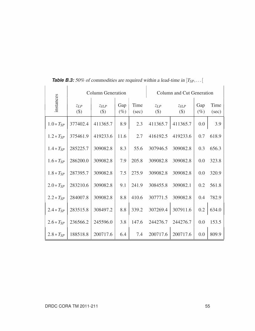
Table B.3: 50% of commodities are required within a lead-time in [TSP, . . . [
inst
ance
s Column Generation Column and Cut Generation
zLP zILP Gap Time zLP zILP Gap Time
($) ($) (%) (sec) ($) ($) (%) (sec)
1.0∗TSP 377402.4 411365.7 8.9 2.3 411365.7 411365.7 0.0 3.9
1.2∗TSP 375461.9 419233.6 11.6 2.7 416192.5 419233.6 0.7 618.9
1.4∗TSP 285225.7 309082.8 8.3 55.6 307946.5 309082.8 0.3 656.3
1.6∗TSP 286200.0 309082.8 7.9 205.8 309082.8 309082.8 0.0 323.8
1.8∗TSP 287395.7 309082.8 7.5 275.9 309082.8 309082.8 0.0 320.9
2.0∗TSP 283210.6 309082.8 9.1 241.9 308455.8 309082.1 0.2 561.8
2.2∗TSP 284007.8 309082.8 8.8 410.6 307771.5 309082.8 0.4 782.9
2.4∗TSP 283515.8 308497.2 8.8 339.2 307269.4 307911.6 0.2 634.0
2.6∗TSP 236566.2 245596.0 3.8 147.6 244276.7 244276.7 0.0 153.5
2.8∗TSP 188518.8 200717.6 6.4 7.4 200717.6 200717.6 0.0 809.9
DRDC CORA TM 2011-211 55

Table B.4: 80% of commodities are required within a lead-time in [TSP, . . . [
inst
ance
s Column Generation Column and Cut Generation
zLP zILP Gap Time zLP zILP Gap Time
($) ($) (%) (sec) ($) ($) (%) (sec)
1.0∗TSP 521630.6 562641.6 7.8 1.8 562641.7 562641.7 0.0 3.88
1.2∗TSP 520176.1 556559.3 6.9 1.8 556559.3 556559.3 0.0 4.4
1.4∗TSP 378842.1 409580.2 8.1 153.1 409580.2 409580.2 0.0 462.5
1.6∗TSP 403497.8 378842.1 6.5 399.7 403497.8 403497.8 0.0 442.4
1.8∗TSP 379888.3 403497.8 6.2 989 403497.8 403497.8 0.0 1302.7
2.0∗TSP 361087.2 386506.4 7.0 1441 383800 386506.4 0.7 1461.6
2.2∗TSP 363241.3 385920.7 6.2 2294.7 384567.7 385920.7 0.3 2948.4
2.4∗TSP 362269.9 389547.5 7.5 2099.6 378052.8 384135.2 1.6 2662.9
2.6∗TSP 309555.9 319941.1 3.3 706.4 319941.1 319941.1 0.0 729.3
2.8∗TSP 189059 200717.6 6.6 10.5 200717.6 200717.6 0.0 555.2
56 DRDC CORA TM 2011-211

Table B.5: 100% of commodities are required within a lead-time in [TSP, . . . [
inst
ance
s Column Generation Column and Cut Generation
zLP zILP Gap Time zLP zILP Gap Time
($) ($) (%) (sec) ($) ($) (%) (sec)
1.0∗TSP 631363.6 741818.1 17.4 1.3 741818.1 741818.1 0.0 2.41
1.2∗TSP 615340.9 720000.0 17.0 1.5 698181.8 698181.8 0.0 3.3
1.4∗TSP 435248.3 460358.8 5.7 488.5 460358.8 460358.8 0.0 497.9
1.6∗TSP 436643.3 460358.8 5.4 2906 60358.8 460358.8 0.0 2932.7
1.8∗TSP 438212.7 460358.8 5.0 4820 460358.8 460358.8 0.0 5332.1
2.0∗TSP 415356.2 440326.1 6.0 13662.8 440326.2 440326.2 0.0 3696.2
2.2∗TSP 416066.7 440326.1 5.8 20174.0 438402.8 440326.1 0.4 20880.5
2.4∗TSP 415236.0 437369.4 5.3 18660.8 437184.4 437369.4 0.0 19563.5
2.6∗TSP 347987.2 352033.8 1.1 1444.0 352033.8 352033.8 0.0 1471.9
2.8∗TSP 188578.2 200717.6 6.4 17.7 200717.6 200717.6 0.0 240.6
3.0∗TSP 188705.0 200717.6 6.3 12.2 200717.6 200717.6 0.0 290.3
DRDC CORA TM 2011-211 57

Table B.6: Percentage of unsafe front-routes in [10%,100%] to be changed
Column Generation Column and Cut Generation
zLP zILP Gap Time zLP zILP Gap Time
($) ($) (%) (sec) ($) ($) (%) (sec)
20% 227115.0 240861.1 6.0 3.6 240861.1 240861.1 0.0 5.0
30% 296326.2 314457 6.1 5.7 314457.6 314457.6 0.0 7.8
50% 427223.2 447974 4.8 11.5 443045.0 447974.6 1.1 921.8
80% 428373.2 447974.6 4.5 5.6 441843.0 447974.6 1.3 662.1
100% 427223 447974 4.8 3.4 447974 447974.6 0.0 28.2
Table B.7: Percentage of unsafe end-routes in [20%,100%] to be changed
Column Generation Column and Cut Generation
zLP zILP Gap Time zLP zILP Gap Time
($) ($) (%) (sec) ($) ($) (%) (sec)
20% 269247.4 287264.7 6.6 4.1 287264.7 287264.7 0.0 242.0
30% 345260.1 365943.8 5.9 6.2 365943.8 365943.8 0.0 9.9
50% 433582.0 460358.8 6.1 4.3 460358.8 460358.8 0.0 273.7
80% 433758.1 460358.8 6.1 3.9 460358.8 460358.8 0.0 5.9
100% 433853.3 460358.8 6.1 3.2 460358.8 460358.8 0.0 264.3
58 DRDC CORA TM 2011-211

DOCUMENT CONTROL DATA(Security classification of title, body of abstract and indexing annotation must be entered when document is classified)
1. ORIGINATOR (The name and address of the organization preparing thedocument. Organizations for whom the document was prepared, e.g. Centre
sponsoring a contractor’s report, or tasking agency, are entered in section 8.)
Defence R&D Canada – CORA
Dept. of National Defence, MGen G.R. Pearkes Bldg.,
101 Colonel By Drive, Ottawa, Ontario, Canada K1A
0K2
2. SECURITY CLASSIFICATION (Overallsecurity classification of the document
including special warning terms if applicable.)
UNCLASSIFIED
3. TITLE (The complete document title as indicated on the title page. Its classification should be indicated by the appropriateabbreviation (S, C or U) in parentheses after the title.)
Design of Tactical Support Strategies in Military Logistics: Trade-offs Between Efficiency and
Effectiveness
4. AUTHORS (Last name, followed by initials – ranks, titles, etc. not to be used.)
Sebbah, S.; Ghanmi, A.; Boukhtouta, A.
5. DATE OF PUBLICATION (Month and year of publication ofdocument.)
December 2011
6a. NO. OF PAGES (Totalcontaining information.Include Annexes,
Appendices, etc.)
76
6b. NO. OF REFS (Totalcited in document.)
40
7. DESCRIPTIVE NOTES (The category of the document, e.g. technical report, technical note or memorandum. If appropriate, enterthe type of report, e.g. interim, progress, summary, annual or final. Give the inclusive dates when a specific reporting period is
covered.)
Technical Memorandum
8. SPONSORING ACTIVITY (The name of the department project office or laboratory sponsoring the research and development –include address.)
Defence R&D Canada – CORA
Dept. of National Defence, MGen G.R. Pearkes Bldg., 101 Colonel By Drive, Ottawa, Ontario,
Canada K1A 0K2
9a. PROJECT NO. (The applicable research and development
project number under which the document was written.Please specify whether project or grant.)
9b. GRANT OR CONTRACT NO. (If appropriate, the applicable
number under which the document was written.)
10a. ORIGINATOR’S DOCUMENT NUMBER (The officialdocument number by which the document is identified by the
originating activity. This number must be unique to thisdocument.)
DRDC CORA TM 2011-211
10b. OTHER DOCUMENT NO(s). (Any other numbers which maybe assigned this document either by the originator or by the
sponsor.)
11. DOCUMENT AVAILABILITY (Any limitations on further dissemination of the document, other than those imposed by security
classification.)
( X ) Unlimited distribution( ) Defence departments and defence contractors; further distribution only as approved
( ) Defence departments and Canadian defence contractors; further distribution only as approved( ) Government departments and agencies; further distribution only as approved( ) Defence departments; further distribution only as approved( ) Other (please specify):
12. DOCUMENT ANNOUNCEMENT (Any limitation to the bibliographic announcement of this document. This will normally correspond
to the Document Availability (11). However, where further distribution (beyond the audience specified in (11)) is possible, a widerannouncement audience may be selected.)

13. ABSTRACT (A brief and factual summary of the document. It may also appear elsewhere in the body of the document itself. It is highlydesirable that the abstract of classified documents be unclassified. Each paragraph of the abstract shall begin with an indication of the
security classification of the information in the paragraph (unless the document itself is unclassified) represented as (S), (C), (R), or (U).It is not necessary to include here abstracts in both official languages unless the text is bilingual.)
Military tactical logistics planning is concerned with the problem of distributing heterogeneous
commodities (e.g., fuel, food, ammunition, etc.) from main operating bases to forward operating
bases in a theatre of operations using a combination of heterogeneous transportation assets
such as logistics trucks and tactical helicopters. Minimizing the sustainment cost while satis-
fying the operational demand under time and security constraints is of high importance for the
Canadian Forces. In this study, a logistics planning model is developed to explore effective and
efficient strategies for tactical logistics distribution. A mathematical optimization algorithm based
on a column and cut generation technique, using Gomory-Chvátal rank−1 cuts, is developed to
solve the problem.
This report presents details of a mathematical formulation and a solution algorithm along with
an example application to demonstrate the methodology. Computational results are presented in
order to measure the degree of efficiency and scalability of the proposed approach, and to study
the trade-off between the efficiency and effectiveness in the resulting sustainment strategies.
14. KEYWORDS, DESCRIPTORS or IDENTIFIERS (Technically meaningful terms or short phrases that characterize a document and could
be helpful in cataloguing the document. They should be selected so that no security classification is required. Identifiers, such asequipment model designation, trade name, military project code name, geographic location may also be included. If possible keywordsshould be selected from a published thesaurus. e.g. Thesaurus of Engineering and Scientific Terms (TEST) and that thesaurus identified.
If it is not possible to select indexing terms which are Unclassified, the classification of each should be indicated as with the title.)
Tactical logistics
Tactical support efficiency
Tactical support effectiveness
Vehicle loading and routing
Optimal fleet mix
Quality-of-Support
Large scale optimization
Column and cut generation
Gomory-Chvátal rank−1 cutting planes


Defence R&D Canada Ca nada's Leader In Defence
a nd Na tional Security Science and Technology
R & D pour la defense Canada Chef de file au Canada en ma tiere de sdence er de rechno logle pour Ia de fense er Ia securlre na tionale
DEFENCE ~EFENSE www.drdc-rddc.gc.ca
Recommended

![arXiv:1604.03649v1 [math.OC] 13 Apr 2016 · Gomory{Johnson model To illustrate what cutting-plane theorems in the Gomory{Johnson model look like, we give three examples of such theorems,](https://img.pdfslide.us/doc/110x75/5b947ea109d3f219658d1111/arxiv160403649v1-mathoc-13-apr-2016-gomoryjohnson-model-to-illustrate.jpg)