472
Journal of Engineering Sciences
Assiut University
Faculty of Engineering
Vol. 43
No. 4
July 2015
PP. 472 – 489
DESIGN OF ROBUST PID CONTROLLERS
FOR FIRST-ORDER PLUS TIME DELAY SYSTEMS
BASED ON FREQUENCY DOMAIN SPECIFICATIONS
Noha Medhat Darwish
Electrical Engineering Dept., Faculty of Engineering, Assiut University, Assiut, Egypt
(Received 6 May 2015; Revised 12 June 2015; Accepted 19 July 2015)
ABSTRACT
This paper considers a design method for PID controllers to achieve the robustness to the uncertainty
of the time delay for the first-order plus time delay system (FOPTD). Initially, the stabilizing regions
of the PID controller gains are determined by a graphical stability method. Then, we specify two
simultaneous design specifications: gain margin and phase crossover frequency. These specifications
give a set of stabilizing PID controllers. To get a unique PID controller, we introduce an additional
constraint which is finding the smallest absolute value of the slope of the open-loop system
magnitude at the specified phase crossover frequency. The obtained PID controller is located in the
stability region, and also robust to system time delay variation due to the proposed constraint.
Keywords: First-Order Plus Time Delay (FOPTD) systems, Gain margin, Proportional-Integral-
Derivative (PID) controllers, Robustness, Stabilizing region.
1. Introduction
Over 90% of the process control and industrial applications are controlled by the
proportional-integral-derivative (PID) controllers [1, 2]. The PID controller has a simple
structure and gives a good performance in the closed-loop response.
Practically, there are several methods for tuning of PID gains such as Ziegler-Nichols
methods [3]. These methods may give a satisfactory closed-loop response, but they cannot
give any information on the stabilizing region of these gains.
The primary aim of the controller design is to maintain the stability of the control system.
There are several methods for computing the stabilizing PID controllers for delay-free linear
time invariant systems [4-8]. However, many of industrial systems have time delay, so the
stable plant that has an S-shaped step response is modeled as first- or second-order plus time
delay models [1].
Several methods for computing the stabilizing PID controllers for the first-order plus
time delay (FOPTD) systems are proposed by the authors of [4, 6, 9-11]. In [4, 6, and 10],
an extension of the Hermite-Biehler Theorem based on Pontryagin results [12] was
investigated to determine all the stabilizing PID controllers. An alternative way is proposed
473
JES, Assiut University, Faculty of Engineering, Vol. 43, No. 4, July 2015, pp. 472 – 489
in [4, 6] using the generalized Nyquist stability criterion. In [9], the stabilizing regions of
the PID gains are obtained by the graphical stability criterion for the FOPTD systems.
As the stability is an important goal for designing the PID controllers, but it is not enough
requirement to get a satisfactory response behavior (robustness and performance). Robust
control is an area of intensive research. It can be achieved using gain and phase margin
specifications [9, 13-15] or closed-loop sensitivity constraint. The sensitivity constraint is
similar with the gain and phase margin specifications as they have a direct relation [1, 16]. In
[13], simple tuning rules for designing PID controller are obtained to satisfy optimal gain and
phase margins. In [14], the robustness is achieved by gain and phase margins while the
closed-loop performance is achieved by bandwidth and maximum amplitude ratio. The
limitation of this work is the nonlinear optimization problem which needs numerical
solution. In [9, 15], the robust design is proposed by achieving the pre-specifications of phase
margin and gain crossover frequency in addition to the flat phase tuning constraint. The
obtained controller has two properties: first, its gains are located in the stabilizing region.
Second, it is robust to a bounded variation in the system gains, which include the uncertainty
of the plant steady-state gain and the overall variations of the controller gains.
Uncertainty in dc gain of the model is important but in dealing with time delay plants,
uncertainty in time delay is more important and critical. In this paper, we consider the
problem of time delay uncertainty by proposing a method to design PID controllers to
achieve the pre-specifications of gain margin, phase crossover frequency, and a minimum
absolute value of the derivative of the open-loop system magnitude with respect to the
frequency at the specified phase crossover frequency based on the FOPTD systems. This
minimum derivative ensures the robustness to a bounded variation in the system time delay
and makes the closed-loop system more robust than the method proposed by the authors of
[13]. For a specified gain margin, choosing a value for the phase crossover frequency
affects on the location of PID gains in the stabilizing region, so the closed-loop robustness
and performance can be adjusted.
As a starting point, all stabilizing PID controllers are determined using a graphical
stability method which is a simple algorithm. Then, we obtain the three dimension relative
stability regions that satisfy the designed gain margin. It is necessary to determine these
stabilizing regions because the first aim of the proposed method is to get a set of stabilizing
PID controllers that guarantee two simultaneous design specifications: gain margin and
phase crossover frequency. From this set, we search for the smallest rate of change of the
open-loop magnitude at the specified phase crossover frequency point cw to get a unique PID
controller which is the second aim.
The contributions of this paper can be summarized as follows:
(1) It considers a design method that makes the closed-loop system more robust than
the method proposed in [13] due to the smallest slope constraint at the specified
phase crossover frequency.
(2) It treats the problem of time delay uncertainty which was not considered in [9, 15].
(3) It proposes a simple approach that provides a satisfactory response behavior
(performance and robustness) that it does not require numerical solution for the
nonlinear optimization as in [14].
474
Noha Medhat Darwish, Design of robust PID controllers for first-order plus time delay ……….
This paper is organized as follows: In the next section, stabilizing and robust PID
controller design is presented. Then, an illustrative example is given. Conclusion is
provided in the last section.
2. Stabilizing and robust PID controller design for FOPTD systems
2.1. FOPTD systems and PID controller
The design method proposed in this paper is based on the FOPTD systems which is
mathematically described by the transfer function,
Lse
Ts
KsG
)1()( (1)
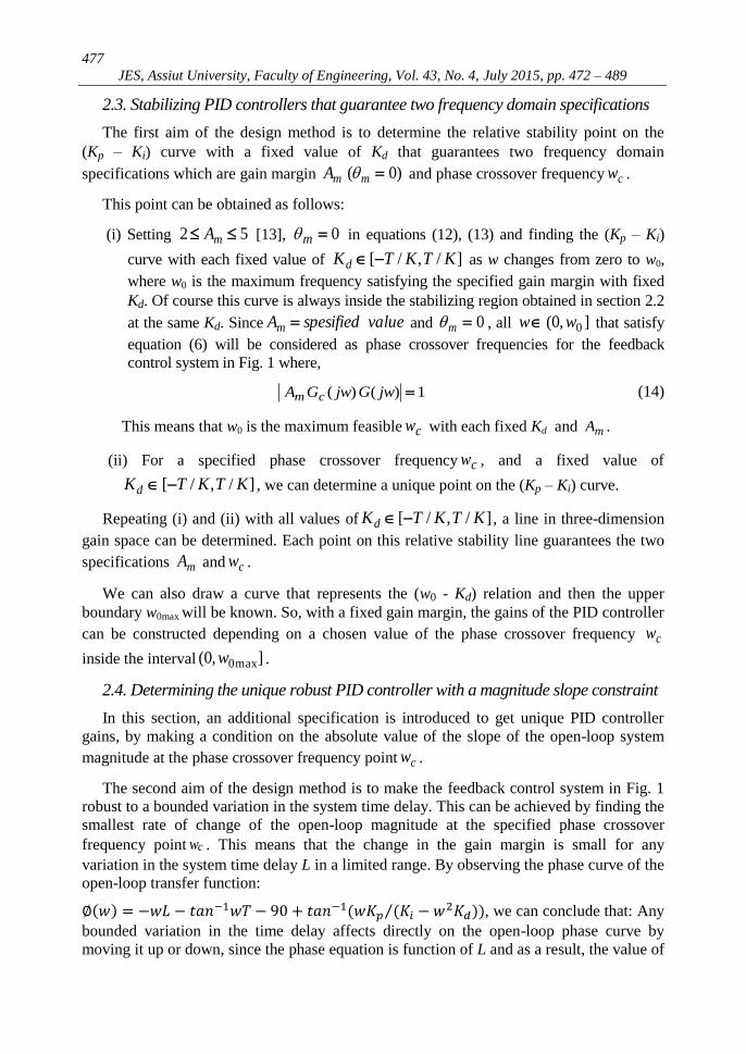
Consider the feedback control system as shown in Fig. 1 with a gain-phase margin
tester [17], where G(s) is the FOPTD plant and )(sGc is the designed PID controller with
the transfer function,
s
KsKsKsG
ipdc
2
)( (2)
where, dK is the derivative gain, pK is the proportional gain, and iK is the integral gain.
The gain-phase margin tester is represented by the frequency independent transfer
function mjm eA
. It provides information for plotting the boundaries of all stabilizing PID
controller gains that achieve specified gain and phase margins [18].
Fig. 1. Feedback control system with gain-phase tester.
For design specification on the gain margin mA , we set 0m , and for design
specification on the phase margin m , we set 1mA .
2.2. Stabilizing region of the PID gains
From Fig. 1, the closed-loop transfer function is:
)()(1
)()()(
sGsGeA
sGsGeAsT
cj
m
cj
m
m
m
(3)
So, the characteristic polynomial will be as follows:
0)()(1)(
sGsGeAs cj
mm (4)
Gc(s) G(s)
+ )(tr
)(ty
mjm eA

475
JES, Assiut University, Faculty of Engineering, Vol. 43, No. 4, July 2015, pp. 472 – 489
By substituting equations (1) and (2) into equation (4), we obtain
)()1()( 2ipd
Lsjm KsKsKeeKATsss m
)( 22ipd
Lsjm KsKsKeeKAsTs m
0 (5)
Determining all the stabilizing PID controllers for the FOPTD plant is a primary aim in
controller design. The closed-loop system is stable if all the roots locations of the
polynomial in equation (5) with 1mA and om 0 are in the left-half of the s-plane. The
location of these roots depends on the PID gains which are Kd, Kp, and Ki. The boundaries
of these gains can be determined by the infinity root boundary (IRB), real root boundary
(RRB) and complex root boundary (CRB) [18-20].
(i) IRB: 0)( s , so we get a boundary on Kd as:
K
TKd
This boundary can be obtained as follow:
Put 0)( s , so the coefficient of 𝑠2 will be equal to zero,
0 d
Lsjm KeeKAT m ,
Put ( 1mA and om 0 ), we obtain:
0 Lsd eKKT
𝑒−𝐿𝑠 can be approximated by a first-order or second-order Pade approximation.
For first-order Pade approximation:
Ls
Lse Ls
2
2, then
K
TK
sd
For second-order Pade approximation:
22
22
612
612
sLLs
sLLse Ls
, then K
TK
sd
so we get a boundary on Kd as:
K
TKd
The same result can be obtained using third-order and fourth-order Pade
approximations. This means that Kd will have positive and negative values.
(ii) RRB: 0)0( s , so we get a boundary on Ki as:
Ki = 0

476
Noha Medhat Darwish, Design of robust PID controllers for first-order plus time delay ……….
(iii) CRB: )( jws , the resulting polynomial will be as follows:
0)()()( 2)(2
ipd
wLjm KjwKKweAKjwwTjw m
0))()sin()(cos()( 22 ipdmmm KjwKKwwLjwLAKjwwT (6)
The real part R (w) and the imaginary part I(w) are as follows:
0))cos()()sin(()( 22 midmpm wLKKwwLwKAKwTwR (7)
0))cos()sin()(()( 2 mpmidm wLKwwLKKwAKwwI (8)
It is clear that from equations (7) and (8) both the real as well as the imaginary parts of
)( jw depend on dK , pK , and iK , which causes difficulties when trying to find the
range of these gains that make the system stable. To overcome this problem, we will now
multiply the characteristic polynomial of equation (6) by )( mwLj
e
for which only the
imaginary part of the resulting polynomial depends on pK only.
Multiply equation (6) by )( mwLj
e
,
0)()()( 22)()(
ipdm
wLjwLjKjwKKwAKjwwTejwe mm
)()())sin()(cos( 22ipdmmm KjwKKwAKjwwTwLjwL
0)Im()Re( wjw (9)
where Re(w) is the real part and Im(w) is the imaginary part as follows:
wLwwLwTw m sin()cos()Re( 2 0) 2 imdmm KKAKwAK (10)
0)sin()cos()Im( 2 pmmm KwAKwLwTwLww (11)
Equating the real part and the imaginary part to zero, we obtain:
pKm
mm
AK
wLwLwT )cos()sin( (12)
iKd
m
mm KwAK
wLwTwLw 22 )cos()sin(
(13)
For each fixed value of Kd, we can determine the values of Kp and Ki as w changes from
zero to infinity using equations (12), (13) and plot the curve of Ki versus Kp that describes
these values. This curve divides the two-dimension space (Kp – Ki) into stable and unstable
regions by RRB and CRB. The stabilizing region can be determined by choosing an
arbitrary point in each region. Mathematically, equation (12) can give positive and
negative values of Kp that stabilize the FOPTD system depending on the values of w.
By sweeping over all values of ]/,/[ KTKTKd , we can determine all the three-
dimension stabilizing regions for the PID controller gains.
477
JES, Assiut University, Faculty of Engineering, Vol. 43, No. 4, July 2015, pp. 472 – 489
2.3. Stabilizing PID controllers that guarantee two frequency domain specifications
The first aim of the design method is to determine the relative stability point on the
(Kp – Ki) curve with a fixed value of Kd that guarantees two frequency domain
specifications which are gain margin )0( mmA and phase crossover frequency cw .
This point can be obtained as follows:
(i) Setting 52 mA [13], 0m in equations (12), (13) and finding the (Kp – Ki)
curve with each fixed value of ]/,/[ KTKTKd as w changes from zero to w0,
where w0 is the maximum frequency satisfying the specified gain margin with fixed
Kd. Of course this curve is always inside the stabilizing region obtained in section 2.2
at the same Kd. Since valuespesifiedAm and 0m , all ],0( 0ww that satisfy
equation (6) will be considered as phase crossover frequencies for the feedback
control system in Fig. 1 where,
1)()( jwGjwGA cm
(14)
This means that w0 is the maximum feasible cw with each fixed Kd and mA .
(ii) For a specified phase crossover frequency cw , and a fixed value of
]/,/[ KTKTKd , we can determine a unique point on the (Kp – Ki) curve.
Repeating (i) and (ii) with all values of ]/,/[ KTKTKd , a line in three-dimension
gain space can be determined. Each point on this relative stability line guarantees the two
specifications mA and cw .
We can also draw a curve that represents the (w0 - Kd) relation and then the upper
boundary w0max will be known. So, with a fixed gain margin, the gains of the PID controller
can be constructed depending on a chosen value of the phase crossover frequency cw
inside the interval ],0( max0w .
2.4. Determining the unique robust PID controller with a magnitude slope constraint
In this section, an additional specification is introduced to get unique PID controller
gains, by making a condition on the absolute value of the slope of the open-loop system
magnitude at the phase crossover frequency point cw .
The second aim of the design method is to make the feedback control system in Fig. 1
robust to a bounded variation in the system time delay. This can be achieved by finding the
smallest rate of change of the open-loop magnitude at the specified phase crossover
frequency point cw . This means that the change in the gain margin is small for any
variation in the system time delay L in a limited range. By observing the phase curve of the
open-loop transfer function:
∅(𝑤) = −𝑤𝐿 − 𝑡𝑎𝑛−1𝑤𝑇 − 90 + 𝑡𝑎𝑛−1(𝑤𝐾𝑝 (𝐾𝑖 − 𝑤2𝐾𝑑))⁄ , we can conclude that: Any
bounded variation in the time delay affects directly on the open-loop phase curve by
moving it up or down, since the phase equation is function of L and as a result, the value of

478
Noha Medhat Darwish, Design of robust PID controllers for first-order plus time delay ……….
the gain margin will be changed. This change is due to the variation in the phase crossover
frequency value. If the absolute value of the slope of the magnitude curve at the specified
phase crossover frequency cw is small, so the variation in the gain margin value is small
and the closed-loop step response is still have a good performance, and the robustness
property is achieved.
Equate equations (7) and (8) and put 0m , we obtain
)15(
))sin()()cos()sin()cos()((
2
22
wTw
wLKKwwLwKwLKwwLKKwAK idppidm
Then the gain margin equation will be as follows:
))cos()(sin())sin())(cos((( 2
2
wLwLKwwLwLKKwK
wTwA
pidm
(16)
Since mc AGG /1 , then
wTw
wLwLKwwLwLKKwKjwGjwG
pidc
2
2 ))cos()(sin())sin())(cos((()()( (17)
From equation (17), we can get,
22 )(
))sin(2)cos(1()()(
wTw
wLEwLEK
dw
jwGjwGd c
(18)
where,
ipd KTLwLTwKTLwLTwKLwLTwwE )1)2(())(()(1 223342 ,
ipd KTLwLTwKTLwLTwKLwLTwwE )1)2(())(()(2 223342
As discussed in section 2.3, all PID gains points on the relative stability line that
guarantee the two specifications mA and cw will be substituted in equation (18) and the
values of this equation are computed at these gains. Then we search among these values
for the smallest one. The resulting PID controller makes the closed-loop system in Fig. 1
robust to bounded system time delay variation. In some cases, the designed PID controller
may give phase margin greater than 70 degree (very slow closed-loop step response) or
less than 30 degree (oscillatory closed-loop step response), so we need to search for the
smallest magnitude slope with a condition on the phase margin range to be om
o 7030 .
Although in this case, the slope is not the minimum value which means the degree of
robustness is reduced, but the robustness is still preserved with a good performance.
479
JES, Assiut University, Faculty of Engineering, Vol. 43, No. 4, July 2015, pp. 472 – 489
3. An illustrative example
Consider a FOPTD system described by the transfer function )1(
)(3.0
s
esG
s
We will apply the proposed method to get the robust PID controller as follows:
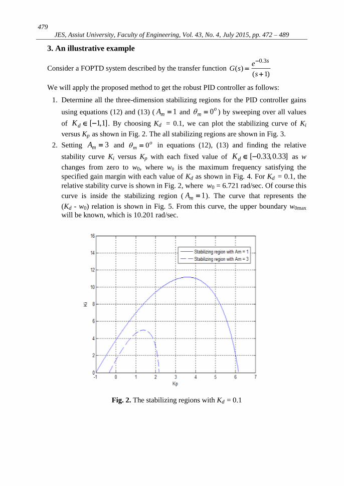
1. Determine all the three-dimension stabilizing regions for the PID controller gains
using equations (12) and (13) ( 1mA and o
m 0 ) by sweeping over all values
of ]1,1[dK . By choosing Kd = 0.1, we can plot the stabilizing curve of Ki
versus Kp as shown in Fig. 2. The all stabilizing regions are shown in Fig. 3.
2. Setting 3mA and om 0 in equations (12), (13) and finding the relative
stability curve Ki versus Kp with each fixed value of ]33.0,33.0[dK as w
changes from zero to w0, where w0 is the maximum frequency satisfying the
specified gain margin with each value of Kd as shown in Fig. 4. For Kd = 0.1, the
relative stability curve is shown in Fig. 2, where w0 = 6.721 rad/sec. Of course this
curve is inside the stabilizing region ( 1mA ). The curve that represents the
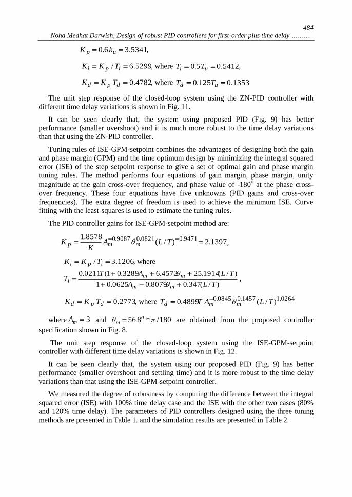
(Kd - w0) relation is shown in Fig. 5. From this curve, the upper boundary w0max
will be known, which is 10.201 rad/sec.
Fig. 2. The stabilizing regions with Kd = 0.1
480
Noha Medhat Darwish, Design of robust PID controllers for first-order plus time delay ……….
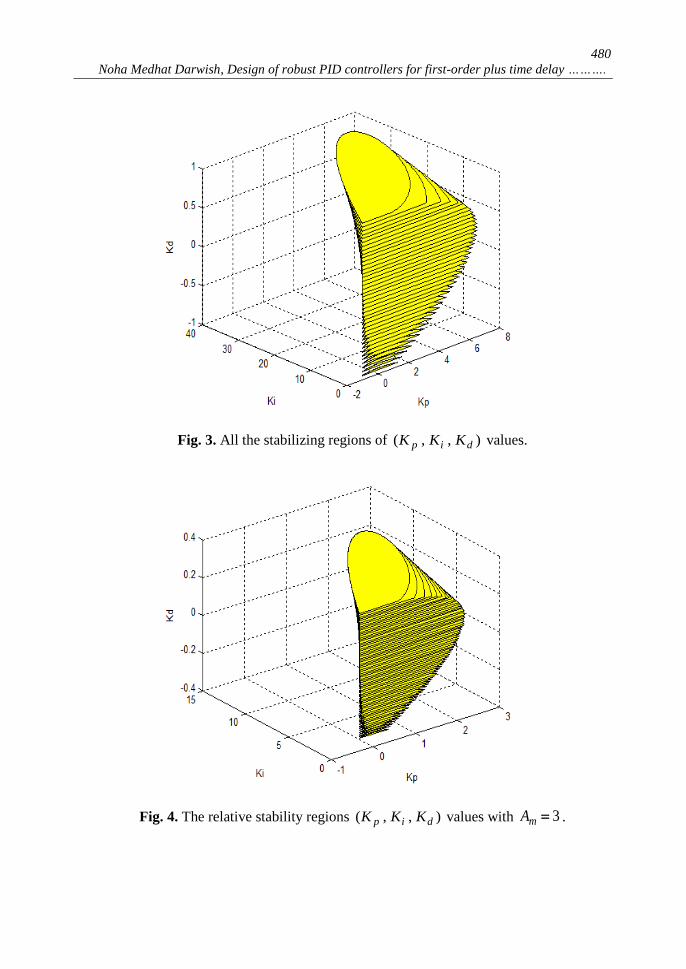
Fig. 3. All the stabilizing regions of ),,( dip KKK values.
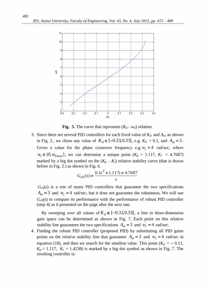
Fig. 4. The relative stability regions ),,( dip KKK values with 3mA .
481
JES, Assiut University, Faculty of Engineering, Vol. 43, No. 4, July 2015, pp. 472 – 489
Fig. 5. The curve that represents (Kd - w0) relation.
3. Since there are several PID controllers for each fixed value of Kd and Am as shown
in Fig. 2., we chose any value of ]33.0,33.0[dK , e.g. Kd = 0.1, and 3mA .
Given a value for the phase crossover frequency e.g. 4cw rad/sec, where
],0( max0wwc , we can determine a unique point (Kp = 1.117, Ki = 4.7687)
marked by a big dot symbol on the (Kp – Ki) relative stability curve (that is drawn
before in Fig. 2.) as shown in Fig. 6.
s
sssGc
7687.4117.11.0)(
2
0
Gc0(s) is a one of many PID controllers that guarantee the two specifications
3mA and 4cw rad/sec, but it does not guarantee the robustness. We will use
Gc0(s) to compare its performance with the performance of robust PID controller
(step 4) as it presented on the page after the next one.
By sweeping over all values of ]33.0,33.0[dK , a line in three-dimension
gain space can be determined as shown in Fig. 7. Each point on this relative
stability line guarantees the two specifications 3mA and 4cw rad/sec.
4. Finding the robust PID controller (proposed PID) by substituting all PID gains
points on the relative stability line that guarantee 3mA and 4cw rad/sec in
equation (18), and then we search for the smallest value. This point (Kd = − 0.11,
Kp = 1.117, Ki = 1.4238) is marked by a big dot symbol as shown in Fig. 7. The
resulting controller is:

482
Noha Medhat Darwish, Design of robust PID controllers for first-order plus time delay ……….
s
sssG proposedc
4238.1117.111.0)(
2
The bode plots of the open-loop transfer functions with Gc0(s) and the robust PID
controller Gc-proposed(s) are shown in Fig. 8. It is clear that, the absolute value of the slope of
the magnitude curve using Gc-proposed(s) at the specified phase crossover frequency 4cw
rad/sec is smaller than that using Gc0(s). It is also clear that, the desired gain margin value is
achieved using both PID controllers (20log 3 = 9.54 dB) at 4cw rad/sec.
Fig. 6. The ),( ip KK point with Kd = 0.1 that satisfies 3mA and 4cw rad/sec.
Fig. 7. The smallest magnitude slope point on the relative stability line with 3mA
and 4cw rad/sec.

483
JES, Assiut University, Faculty of Engineering, Vol. 43, No. 4, July 2015, pp. 472 – 489
Fig. 8. The bode plots of the open-loop transfer functions.
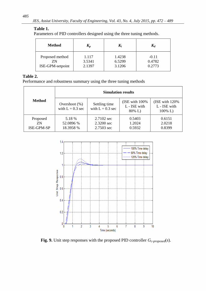
The unit step response of the closed-loop system using the proposed PID controller
Gc-proposed(s) with different time delay variations is shown in Fig. 9. It is clear that the
effect of the variation in the system time delay by %20 on the step response is small.
This means that the robustness is achieved.
The unit step response of the closed-loop system using another PID controller Gc0(s)
with different system time delay variations is shown in Fig. 10. It is shown that the effect
of the variation in the time delay by %20 on the step response is large and the robustness
is not achieved.
A comparison is made with two different methods. We computed the PID controllers
using the Ziegler-Nichols frequency response method [1, 3] and the PID controller using
the tuning rules for setpoint (ISE-GPM-setpoint) [13].
Ziegler-Nichols method is based on a simple characterization of the process dynamics.
The design is based on knowledge of the point on the Nyquist curve of the process transfer
function G(s) where the Nyquist curve intersects the negative real axis. This point is
characterized by the parameters Ku and Tu which are called the ultimate gain and the
ultimate period. Ziegler-Nichols gives simple formulas for the gains of the PID controller
in terms of the ultimate gain and the ultimate period.
The parameters of Ziegler-Nichols frequency response method will be as follows:
uk = 5.8902, uw = 5.8047 rad/sec,
and 1.0824 /2 uu wT sec
The PID controller gains are:
484
Noha Medhat Darwish, Design of robust PID controllers for first-order plus time delay ……….
3.53416.0 up kK ,
6.5299 / ipi TKK , where 0.5412 5.0 ui TT ,
0.4782 dpd TKK , where 0.1353 125.0 ud TT
The unit step response of the closed-loop system using the ZN-PID controller with
different time delay variations is shown in Fig. 11.
It can be seen clearly that, the system using proposed PID (Fig. 9) has better
performance (smaller overshoot) and it is much more robust to the time delay variations
than that using the ZN-PID controller.
Tuning rules of ISE-GPM-setpoint combines the advantages of designing both the gain
and phase margin (GPM) and the time optimum design by minimizing the integral squared
error (ISE) of the step setpoint response to give a set of optimal gain and phase margin
tuning rules. The method performs four equations of gain margin, phase margin, unity
magnitude at the gain cross-over frequency, and phase value of -180o at the phase cross-
over frequency. These four equations have five unknowns (PID gains and cross-over
frequencies). The extra degree of freedom is used to achieve the minimum ISE. Curve
fitting with the least-squares is used to estimate the tuning rules.
The PID controller gains for ISE-GPM-setpoint method are:
1397.2)/(8578.1 9471.00821.09087.0 TLAK
K mmp ,
3.1206 / ipi TKK , where
)/(347.08079.00625.01
)/(1914.254572.63289.01(0211.0
TLA
TLATT
mm
mmi
,
0.2773 dpd TKK , where 0264.11457.00845.0 )/(4899.0 TLATT mmd
where 3mA and 180/*8.56 om are obtained from the proposed controller
specification shown in Fig. 8.
The unit step response of the closed-loop system using the ISE-GPM-setpoint
controller with different time delay variations is shown in Fig. 12.
It can be seen clearly that, the system using our proposed PID (Fig. 9) has better
performance (smaller overshoot and settling time) and it is more robust to the time delay
variations than that using the ISE-GPM-setpoint controller.
We measured the degree of robustness by computing the difference between the integral
squared error (ISE) with 100% time delay case and the ISE with the other two cases (80%
and 120% time delay). The parameters of PID controllers designed using the three tuning
methods are presented in Table 1. and the simulation results are presented in Table 2.
485
JES, Assiut University, Faculty of Engineering, Vol. 43, No. 4, July 2015, pp. 472 – 489
Table 1. Parameters of PID controllers designed using the three tuning methods.
Method Kp Ki Kd
Proposed method
ZN
ISE-GPM-setpoint
1.117
3.5341
2.1397
1.4238
6.5299
3.1206
-0.11
0.4782
0.2773
Table 2. Performance and robustness summary using the three tuning methods
Method
Simulation results
Overshoot (%)
with L = 0.3 sec
Settling time
with L = 0.3 sec
(ISE with 100%
L - ISE with
80% L)
(ISE with 120%
L - ISE with
100% L)
Proposed
ZN
ISE-GPM-SP
5.18 %
52.0896 %
18.3958 %
2.7102 sec
2.3200 sec
2.7503 sec
0.5403
1.2024
0.5932
0.6151
2.0218
0.8399
Fig. 9. Unit step responses with the proposed PID controller Gc-proposed(s).

486
Noha Medhat Darwish, Design of robust PID controllers for first-order plus time delay ……….
Fig. 10. Unit step responses with PID controller Gc0(s)
Fig. 11. Unit step responses with ZN-PID controller.

487
JES, Assiut University, Faculty of Engineering, Vol. 43, No. 4, July 2015, pp. 472 – 489
Fig. 12. Unit step responses with ISE-GPM-setpoint controller.
4. Conclusion
This paper considers the design method for PID controllers to achieve the robustness to
the uncertainty of the time delay for the first-order plus time delay system (FOPTD). We
first determine the stabilizing regions of the PID controller gains by a graphical stability
method. Then, we specify two simultaneous design specifications: gain margin and phase
crossover frequency. To get a unique PID controller, an additional constraint on the
magnitude slope is introduced, by searching for the smallest absolute value of the
derivative of the open-loop system magnitude with respect to the frequency at the specified
phase crossover frequency. The obtained PID controller is located in the stability region,
and also robust to system time delay variation due to that constraint.
The design steps of the proposed method are summarized in an example. It is shown in
the illustrative example that the proposed method gives better performance (smaller
overshoot) for the unit step response than that in the ZN method and GPM-ISE method.
Also, the proposed PID controller is more robust to a bounded variation in the system time
delay than that using ZN and GPM-ISE controllers.
REFERENCES
[1] K. Astrom and T. Hagglund, PID Controllers: Theory, Design, and Tuning, Research
Triangle Park: Instrument Society of America, 1995.
[2] K. Astrom and T. Hagglund, Advanced PID Control, Research Triangle Park: Instrument
Society of America, 2005.
[3] J. G. Ziegler and N. Nichols, “Optimum settings for automatic controllers”, Transactions of
the ASME, vol. 64, no. 8, pp. 759-768, 1942.
[4] S. P. Bhattacharyya, A. Datta, and L. H. Keel, Linear Control Theory: Structure,
Robustness and Optimization. Taylor & Francis Group, 2009.

488
Noha Medhat Darwish, Design of robust PID controllers for first-order plus time delay ……….
[5] A. I. Saleh, M. M. Hasan, and N. M. Darwish, “Determination of Controllers Gains Limit
Using The Mikhailov Stability Criterion”, Journal of Engineering Sciences, Assiut
University, Egypt, vol. 38, no. 1, pp. 209-219, 2010.
[6] G. J. Silva, A. Datta A, and S. P. Bhattacharyya, PID Controllers for Time-Delay Systems.
Boston: Birkhӓuser, 2005.
[7] N. Tan and I. Kaya, “Computation of stabilizing PI and PID controllers”, In Proceedings of
IEEE Conference on Control Applications, vol. 2, pp. 876-881, 2003.
[8] N. Tan, I. Kaya, C. Yeroglu, et al. “Computation of stabilizing PI and PID controllers using
the stability boundary locus”, Energy Conversion and Management, vol. 47, no. (18-19),
pp. 3045-3058, 2006.
[9] Y. Luo and Y.Q. Chen, “Synthesis of robust PID controllers design with complete
information on pre-specifications for the FOPTD systems”, In Proceedings of American
Control Conference, pp. 5013-5018, 2011.
[10] G. J. Silva, A. Datta A, and S. P. Bhattacharyya, “New Results on the Synthesis of PID
Controller”, IEEE Transaction on Automatic Control, vol. 47, no. 9, pp. 241-252, 2002.
[11] D. J. Wang, “Further results on the synthesis of PID controllers”, IEEE Transaction on
Automatic Control, vol. 52, no. 6, pp. 1127-1132, 2007.
[12] L. S. Pontryagin,” On the zeros of some elementary transcendental function (in English)”,
American Mathematical Society Translation, vol. 2, pp. 95-110, 1955.
[13] W. K. HO, K. W. LIM, and W. XU, “Optimal Gain and Phase Margin Tuning for PID
Controllers”, Automatica, vol.34, no. 8, pp. 1009-1014, 1998.
[14] K. Li, “PID Tuning for Optimal Closed-Loop Performance With Specified Gain and Phase
Margins”, IEEE Transaction on Control Systems Technology, vol. 21, no. 3, pp. 1024-
1030, 2013.
[15] Y. Luo and Y.Q. Chen, “Stabilizing and robust fractional order PI controller synthesis for
first order plus time delay systems”, Automatica, vol. 48, no. 9, pp. 2159-2167, 2012.
[16] J. Qibing, L. Qie, W. Qi, et al, “PID Controller Design Based on the Time Domain
Information of Robust IMC Controller Using Maximum Sensitivity”, Chinese Journal of
Chemical Engineering, vol. 21, no. 5, pp. 529-536, 2013.
[17] C. H. Chang and K. W. Han, “Gain margins and phase margins for control systems with
adjustable parameters”, Journal of Guidance, Control, and Dynamics, vol. 13, no. 3, pp.
404-408, 1990.
[18] S. E. Hamamci, “An algorithm for stabilization of fractional-order time delay systems
using fractional-order PID controllers”, IEEE Transaction on Automatic Control, vol. 52,
no. 10, pp. 1964–1969, 2007.
[19] J. Ackermann and D. Kaesbauer, “Stable polyhedral in parameter space”, Automatica, vol.
39, no. 5, pp. 937- 943, 2003.
[20] S. E. Hamamci, and N. Tan, “Design of PI controllers for achieving time and frequency
domain specifications simultaneously”, ISA Transaction, vol. 45, no. 4, pp. 529-543, 2006.

489
JES, Assiut University, Faculty of Engineering, Vol. 43, No. 4, July 2015, pp. 472 – 489
تصميم المحكمات التناسبية التكاملية التفاضلية المتينة للنظم من
الدرجة األولى ذات التأخير الزمنى بناء على خصائص فى مجال التردد
الملخص العربى:
هذا البحث يتناول طريقة تصميم للمحكمات التناسبية التكاملية التفاضلية لتحقيق المتانة فى حالة التغير الطفيف
. بداية تم ايجاد معامالت المحكمات التناسبية ذو التأخير الزمنى الزمنى للنظام من الدرجة األولى فى التأخير
التكاملية التفاضلية التى تضمن اتزان نظام التحكم باستخدام طريقة االتزان الرسومية. بعد ذلك تم تحديد
وقد نتج عن ذلك مجموعة من درجة ١٨٠خاصيتين للتصميم هما كسب الحد والتردد الذى يحقق زاوية وجه
المحكمات التناسبية التكاملية التفاضلية التى تحقق قيم هاتين الخاصيتين. اليجاد محكم تناسبى تكاملى تفاضلى
المقدار فى مجال التردد لنظام منحنى تم اضافة قيد على القيمة المطلقة لميل ٬وحيد من تلك المجموعة السابقة
وذلك من خالل ايجاد أصغر قيمة مطلقة لهذا ٬درجة ١٨٠دد الذى يحقق زاوية وجه الدائرة المفتوحة عند التر
الميل. هذا المحكم التناسبى التكاملى التفاضلى الذى تم ايجاده يحقق االتزان وفى نفس الوقت يحقق المتانة
لنظام التحكم فى حالة التغير الطفيف فى التأخير الزمنى.
Recommended