DESIGN OF NEXT GENERATION ANTENNA MOUNT
IN TELECOMMUNICATION TOWERS WITH
LOW EFFECTIVE PROJECTED AREA
By
RUBEN GREGORY PUTHOTA DOMINIC SAVIO
Presented to the Faculty of the Graduate School of
The University of Texas at Arlington in Partial Fulfillment
Of the Requirements
For the Degree of
MASTER OF SCIENCE IN MECHANICAL ENGINEERING
THE UNIVERSITY OF TEXAS AT ARLINGTON
August 2015

ii
Copyright © by Ruben Gregory Puthota Dominic Savio 2015
All Rights Reserved

iii
Acknowledgements
Firstly, I would like to thank my professor Dr. Dereje Agonafer who has been an
immense presence in my graduate studies guiding me to complete thesis and mold me
into a professional student with his own experience.
I want to sincerely thank CommScope Inc. for giving me the opportunity to work
on their project and develop that into a thesis. I am also thankful to industry mentors Mr.
Tom Palmer and Mr. Al Skrepcinski for their overall help to finish my thesis.
I also like to thank all EMNSPC lab members and mechanical department who
supported me throughout my graduate studies and helped me get through it all,
particularly Betsegaw Gebrehiwot one of the PhD students, who was like a mentor and a
brother to me, inspired a lot with his urge to learn and willingness to share his knowledge.
I take this opportunity to show my gratitude to Dr. Haji Sheikh and Dr. Ratan
Kumar for being there as my committee members and also thank them for their valuable
comments on my thesis and the work I put in.
Finally, I am also grateful to my parents Mr&Mrs Dominic Savio, brother Amal
Kennedy, sister-in-law Tina and friend Kanimozhi for their unconditional love, patience,
financial backing and mental support to complete my thesis and also my life in general.
July 23, 2015

iv
Abstract
DESIGN OF NEXT GENERATION ANTENNA MOUNT
IN TELECOMMUNICATION TOWERS WITH
LOW EFFECTIVE PROJECTED AREA
Ruben Gregory Puthota Dominic Savio, MS
The University of Texas at Arlington, 2015
Supervising Professor: Dereje Agonafer
Design of new antenna mount with low effective projected area (EPA) and high
load carrying capacity for telecommunication towers is the purpose of this thesis. The
main aim is to reduce the EPA of the mount against the wind pressure direction at the
desired elevation from ground by reducing the mount frame structure parts compared to
the previous mount designs used in the market. The model in itself has to withstand its
dead weight, operator’s weight along with five antenna-radio units. The new model has
been designed with a single horizontal frame and four supporting structure for
EPA reduction and also the EPA is calculated through Image Processing using MATLAB
tool which has not been done previously for mounting structures in the
telecommunication field. The stress and deformation results calculated using ANSYS
15.0 workbench tool and results are analyzed for von-mises stress criterion.

v
Table of Contents
Acknowledgements .............................................................................................................iii
Abstract .............................................................................................................................. iv
List of Illustrations ..............................................................................................................vii
List of Tables ...................................................................................................................... ix
Chapter 1 INTRODUCTION ................................................................................................ 1
1.1. Wireless communication .......................................................................................... 1
1.2. Telecommunication Towers ..................................................................................... 3
1.3. Antenna-RRU mounting structures.......................................................................... 6
1.4. Image Processing .................................................................................................. 10
Chapter 2 ANTENNA-RADIO UNIT MOUNT DESIGN THEORY [6] ................................ 11
2.1. Design Factors....................................................................................................... 11
2.2 Design parameters and Standard calculation [6]. .................................................. 13
2.2.1. Parameters ..................................................................................................... 13
2.2.2 Standard calculation for wind force [6] ............................................................ 14
2.2.2.1. Effective projected area of mounting structure to the
windward face normal to the azimuth of the frame (EPAN) [6] ............................. 14
2.2.2.2 Wind pressure calculation [6] ................................................................... 15
Chapter 3 EFFECTIVE PROJECTED AREA CALCULATION ......................................... 20
3.1. Methodology .......................................................................................................... 20
3.2. Flowchart ............................................................................................................... 20
3.3. Verification of the Method ...................................................................................... 24
Chapter 4 NEW ANTENNA MOUNTING STRUCTURE DESIGN .................................... 28
4.1. Mount CAD model ................................................................................................. 28
4.2. Material Data ......................................................................................................... 31

vi
4.3. Finite Element Model ............................................................................................. 32
4.3.1. Importing CAD model ..................................................................................... 33
4.3.2. Contact analysis ............................................................................................. 34
4.3.3. Meshing the Model ......................................................................................... 35
4.3.4. Boundary Conditions ...................................................................................... 38
Chapter 5 RESULTS ......................................................................................................... 40
5.1. Effective Projected Area results [17] ..................................................................... 40
5.1.1. Effective projected area of frame structures .................................................. 40
5.1.2. Effective Projected Area of supporting structures .......................................... 42
5.2. Finite Element Analysis Results [19] ..................................................................... 44
5.2.1. Stress and Strain Results ............................................................................... 44
5.2.2. Total Deformation Result ................................................................................ 48
Chapter 6 Conclusion ........................................................................................................ 50
References ........................................................................................................................ 51
Biographical Information ................................................................................................... 53

vii
List of Illustrations
Figure 1.1 Nikola Tesla [9] .................................................................................................. 1
Figure 1.3 Monopole Tower [13] ......................................................................................... 3
Figure 1.4 Self-supporting Tower [13] ................................................................................. 4
Figure 1.5 Guyed Tower [13] .............................................................................................. 4
Figure 1.6 Types of telecommunication towers [7] ............................................................. 5
Figure 1.7 Antenna-Radio units .......................................................................................... 5
Figure 1.8 Antenna Solar panel protector ........................................................................... 6
Figure 1.9 Antenna mount carrying four antenna units ....................................................... 7
Figure 1.10 Antenna mount carrying three antenna units................................................... 8
Figure 1.11 Connector plates and bolts .............................................................................. 8
Figure 1.12 Separator flanges ............................................................................................ 9
Figure 1.13 Tower leg connectors ...................................................................................... 9
Figure 1.14 Arrangement of electromagnetic spectrum based on
energy per photon [2] ........................................................................................................ 10
Figure 3.1 Rendering options without changes [18] ......................................................... 21
Figure 3.2 Rendered settings [18] ..................................................................................... 21
Figure 3.3 Flowchart for EPA calculation .......................................................................... 22
Figure 3.4 SF-QV 14-B mount structure [5] ...................................................................... 24
Figure 3.5 SF-QV 14-B mount with background plate [18] ............................................... 24
Figure 3.6 Binary image of frame structure....................................................................... 25
Figure 3.7 Binary image of flat members of supporting structure [17] .............................. 25
Figure 3.8 Binary image of round members of supporting structure [17] ......................... 26
Figure 4.1 Mounting structures with vertical pipes [18] ..................................................... 28
Figure 4.2 Mounting structure with Antenna-Radio units [18] ........................................... 29

viii
Figure 4.3 Frame and supporting structure connection plate [18] .................................... 30
Figure 4.4 Antenna vertical tube connection plate [18] ..................................................... 30
Figure 4.5 Schematic diagram of structural analysis ........................................................ 32
Figure 4.6 Material library in ANSYS workbench 15.0 [19]............................................... 33
Figure 4.7 Imported geometry model ................................................................................ 34
Figure 4.8 Initial contact information ................................................................................. 35
Figure 4.9 Tets, bricks, prism and pyramid mesh elements ............................................. 36
Figure 4.10 Proximity and Curvature mesh method [19] .................................................. 36
Figure 4.11 Detailed view of the meshed mounting structure [19] ................................... 37
Figure 4.12 Boundary conditions [19] ............................................................................... 39
Figure 5.1 Binary image of flat members of frame structure............................................. 41
Figure 5.2 Binary image of round member of frame structure .......................................... 41
Figure 5.3 Binary image of flat members of supporting structures ................................... 42
Figure 5.4 Binary image of round members of supporting structures ............................... 43
Figure 5.5 Von-Mises and maximum shear stress criterion [16]....................................... 44
Figure 5.6 Maximum von-mises stress point [19] ............................................................. 45
Figure 5.7 Detailed view of max stress point [19] ............................................................. 45
Figure 5.8 Detailed front view of the max stress point [19] ............................................... 46
Figure 5.9 Strain result [19] ............................................................................................... 47
Figure 5.10 Detailed view of max-strain point on frame structure [19] ............................. 47
Figure 5.11 Detailed front view of max strain point on frame structure [19] ..................... 48
Figure 5.12 Total Deformation (True scale) [19] ............................................................... 48
Figure 5.13 Magnified view of the deformation [19] .......................................................... 49

ix
List of Tables
Table 2.1 Exposure category ............................................................................................ 16
Table 2.2 Exposure category-continued ........................................................................... 17
Table 2.3 Topographic category ....................................................................................... 17
Table 2.4 Wind probability factor ...................................................................................... 18
Table 2.5 Importance factor .............................................................................................. 18
Table 2.6 Wind pressure details [6] ................................................................................. 19
Table 3.1 Effective projected area [17] ............................................................................. 26
Table 4.1 Material property data ....................................................................................... 31
Table 5.1 EPAMN Result .................................................................................................... 40
Table 5.2 EPAFN Result ..................................................................................................... 42
Table 5.3 EPAN Result ...................................................................................................... 43

1
Chapter 1
INTRODUCTION
1.1. Wireless communication
Wireless communication, one of the most important inventions that the entire 20th
century is said to be surviving with it. Nikola Tesla is considered more like the father of
wireless communication since it all started with his ideology that he proposed to the entire
world. Tesla was born on july 10th 1856 in Croatia who had a great photographic memory.
Telsa is still one of the most underrated among the list of inventors like Thomas Edison,
Marconi and Benjamin Franklin. In his own words [15], “If in a thunderstorm hit earth’s
surface, it creates concentric wave that travels along earth’s crust and comes back to the
original place where it started. Earth’s crust is a conductor of electrical energy because of
the abundance in ion particles and hence we should destroy distance as our senses can
only tell about things nearer but how to know things that are far away. We should be able
to transmit information that is far away and the wireless power transmission concept
should be able to provide free power to all humans who should be able to have power
just like they breather air”.
Figure 1.1 Nikola Tesla [9]
2
In 1890s Tesla built the first model to demonstrate the wireless transmission of
electrical energy where he used a transmitter and a portable receiver at a national level
electrical conference at St. Louis [9]. The first telecommunication tower called the
Wardenclyffe tower [1] was built on long island in 1901 by Tesla with the funding from
businessman J.P. Morgan to test Tesla’s idea of wireless power transmission and
wireless communication at high altitudes where the air is conductive because it’s thinner
[9]. But the first proper telecommunication station, the Telefunken radio station was built
at Sayville, Long Island in 1912 [4].
Wireless communication is one of the fastest growing parts of the
communications industry. The cellular systems usage has been growing in an
exponential rate over the last decade and it has been estimated that there could be
currently 2 billion users worldwide and counting. The demand in cellular systems, laptops
worldwide increases the need and speed of the wireless network. Thus the wireless
systems started to see an evolution from First generation (1G-pcs) usage of analog
communications to Second generation (2G-TDMA/CDMA) systems which moved from
analog to digital which also increased the speed in communication. The 2G systems later
in the 2000s evolved to 3G (WYMAX/EVDO) systems which had higher frequency band
and faster compared to the previous generation systems [2]. The current and emerging
need of wireless network means that the technology involving the Mechanical
engineering, Electrical engineering, Information Engineering, Automation Engineering
also has to be evolved [14].
The evolution in the Mechanical side of wireless communication industry includes
the design Antenna-Radio units and wireless mounting systems without failure. The
increase in demand of the frequency band in turn increases the number of Antenna-
Radio units mounted on a telecommunication tower and so the weight of the whole unit is
3
also higher. Presently the wireless Mount structure holds four Antenna-Radio units to
form one sector. Three such sectors are fixed at the same elevation from the ground level
on the tower to produce an interference of 360ᵒ for the signal frequency. This thesis is
based on the future need of increased bandwidth which could increase the count of the
Antenna-Radio units to five. The increased antenna-radio units will definitely increase the
number of structures used for the design of mount in order to have a better weight
carrying capacity thus increasing the EPA. One of the major parts of the design process
is to calculate and reduce the EPA as low as possible but also without compromising the
mechanical stability of the mount [14].
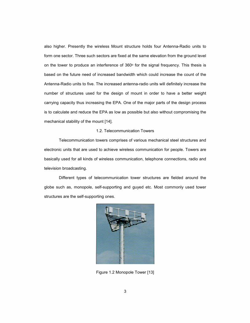
1.2. Telecommunication Towers
Telecommunication towers comprises of various mechanical steel structures and
electronic units that are used to achieve wireless communication for people. Towers are
basically used for all kinds of wireless communication, telephone connections, radio and
television broadcasting.
Different types of telecommunication tower structures are fielded around the
globe such as, monopole, self-supporting and guyed etc. Most commonly used tower
structures are the self-supporting ones.
Figure 1.2 Monopole Tower [13]

4
Figure 1.3 Self-supporting Tower [13]
Figure 1.4 Guyed Tower [13]

5
Figure 1.5 Types of telecommunication towers [7]
Towers can vary in height between 100ft to 2000ft and also depends on the site
whether it is a hill or plain area [11]. Telecommunication towers are manufactured in huge
parts and are erected on site using cranes and could take a month to complete
depending on the tower structure [11]. Towers carry Antennas and Remote radio units to
produce electrical signals and transmit them for usage.
Figure 1.6 Antenna-Radio units

6
One of those advanced antenna mount designs to be used to avoid solar
radiation is shown below.
Figure 1.7 Antenna Solar panel protector
1.3. Antenna-RRU mounting structures
As discussed earlier, a tower will be built to carry on antennas and radio units
that generate signals needed for wireless communication. To fix all those antenna units
we need proper mechanical mounting structures that could hold all the equipment. As the
evolution of wireless communication goes on growing the need to build better mounts are
also necessary and mounting structure are also evolving based on the increase in

7
number of antenna units and its weight. Some of the antenna mounts are shown in the
images. There are different types of antenna mounting structures based on the
requirement. Antenna mounts varies with different numbers of antenna units like two,
three or even four units.
Figure 1.8 Antenna mount carrying four antenna units
Antenna mounts consists of different structures and assembled parts that acts as
a bridge between antenna-radio units and tower legs. Basically, a mounting structure
comprises of main frame structures those hold all the antenna, antenna vertical pipes,
radio units, cables and also main supporting structures that holds the entire frame to
connect them to the tower leg. The connections and the parts used are all well designed
to hold frames, antennas, radio units and fiber optic cables [10]. There are separators
used to hold all frame structures without bumping into other closely fixed sector’s frame
elevated at the same height.
8
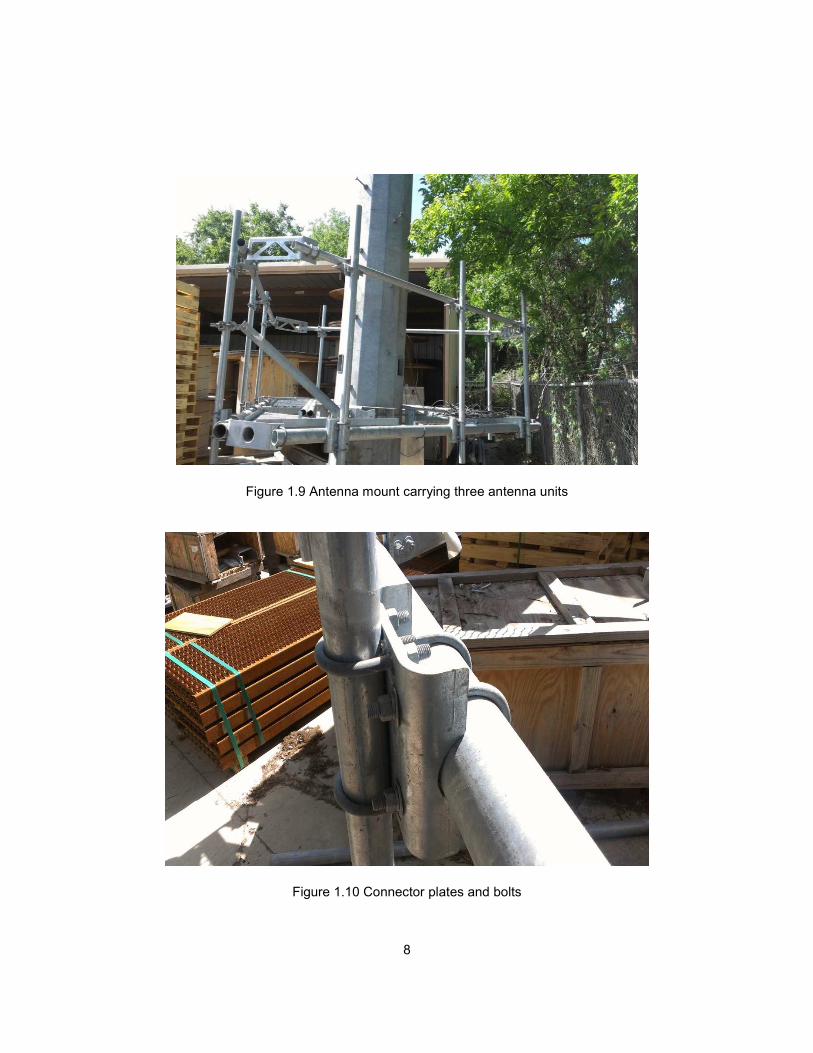
Figure 1.9 Antenna mount carrying three antenna units
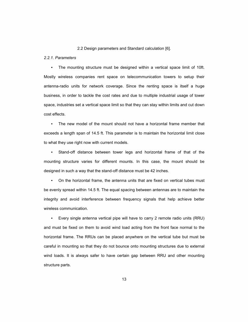
Figure 1.10 Connector plates and bolts

9
Figure 1.11 Separator flanges
All the mounting frames are fixed to tower legs using strong plate structures and
some of the connectors for specific mounting structures will be flexible enough to tilt or
pivot the entire structure to help adjust radio signal frequency and direction.
Figure 1.12 Tower leg connectors

10
1.4. Image Processing
Image processing is one of the methods that can be used to calculate projected
area of mount structures. Image processing has become a major research oriented area
that is used vastly from photography to various fields like computer vision, astrology and
engineering imaging [12]. One of the areas that use image processing is the
differentiation of different wavelength waves.
Figure 1.13 Arrangement of electromagnetic spectrum based on energy per photon [2]
According to Jain [3], digital image processing is an application of function that
transform a two dimensional image using a computer. The main five purpose of image
processing are visualization, Image sharpening, Image retrieval, pattern measurement
and Image recognition [8]. There are two types of Image processing, one the analog and
the other digital. Analog Image processing is used for obtaining hard copies in
photographs and printouts. Digital Image processing uses computer to process images
and one of the biggest flied it is being used is on producing proper satellite images. The
procedure followed to attain the RGB image is to compress the image at first, pre-
processing method for noise filtering, edge extraction. Then the RGB image is converted
to Grey scale image for further measurements or calculations based on requirements.
One of the advanced techniques in image processing is to use parallel processing,
network based processing and artificial intelligence [12]. Some of the current researches
where Image processing is used are brain imaging, cancer imaging and a lot more
medical related areas.

11
Chapter 2
ANTENNA-RADIO UNIT MOUNT DESIGN THEORY [6]
In this chapter, we discuss about all the design requirements, parameters, the
telecommunication standard data to be used in order to design the new Antenna-radio
unit mounting structure to mount antennas on telecommunication towers. The design of
antenna mount structure should be eligible to be mounted on different kinds of
telecommunication towers irrespective of their leg structures. The mounting structure
should be easy to use without any complicated assembly parts, so that it is mountable
using cranes and humans who work on bolt-nut connections.
2.1. Design Factors
The design of new mounting structures has to be done with care not only
because the structures need to support antenna and radio units that make our modern
communication possible but also the people who work on and around the tower need to
conduct their work safely. Hence the following factors need to be considered while
designing the mounting structures:
• Effective Projected Area (EPA)
The antenna-radio mounting assembly can be as high as 70m to 100m above ground
and all of the assembly is expected to be placed within 3m to 3.6m vertical space. At
such height, the wind blows at higher speed than it does close to the ground. To reduce
the wind force applied on the antenna-radio mounting structure, it is important to
minimize the area where wind force is applied to the mounting structure (i.e. the EPA). If
the EPA of the mount is reduced then the weight of the structure that needs to support
the antenna-radio assembly could also be reduced.

12
• Weight carrying capacity
A radio-antenna unit is expected to weigh as much as 1330N. A sector may carry up to
five antenna-radio units and also adding the operating human weight which could be
2224N, the mounting structure for the sector should be designed to carry 8896N dead
load.
• Weight of the mounting structure
The antenna-radio mounting structures are mounted on to the telecommunication towers
by skilled operators using different methods. Currently existing mounting structures,
which are made of hot-dip galvanized carbon steel, are heavy and could become heavier
in the coming years since the structure will be expected to carry more number of and
heavier telecommunication equipment. So the design of new mounting structures should
consider an installation which may involve mounting the members up 70m to 100m above
ground. If possible materials other than steel which are lighter but able to provide
structural support to the antenna-radio assembly and sustain the elements should be
considered.
• Cost
Effort should be made to minimize the life-cycle cost of the new design (purchase,
transportation, etc) and the cost of the new design should not increase significantly
compared to existing mounting structures.
• Specifications
The antenna mount design should meet the ANSI/TIA 222 rev-G standards [6] developed
for telecommunication towers. The parameters and wind load condition data should be
used as per the standards. The materials to be selected should always maintain ASME
standard.
13
2.2 Design parameters and Standard calculation [6].
2.2.1. Parameters
• The mounting structure must be designed within a vertical space limit of 10ft.
Mostly wireless companies rent space on telecommunication towers to setup their
antenna-radio units for network coverage. Since the renting space is itself a huge
business, in order to tackle the cost rates and due to multiple industrial usage of tower
space, industries set a vertical space limit so that they can stay within limits and cut down
cost effects.
• The new model of the mount should not have a horizontal frame member that
exceeds a length span of 14.5 ft. This parameter is to maintain the horizontal limit close
to what they use right now with current models.
• Stand-off distance between tower legs and horizontal frame of that of the
mounting structure varies for different mounts. In this case, the mount should be
designed in such a way that the stand-off distance must be 42 inches.
• On the horizontal frame, the antenna units that are fixed on vertical tubes must
be evenly spread within 14.5 ft. The equal spacing between antennas are to maintain the
integrity and avoid interference between frequency signals that help achieve better
wireless communication.
• Every single antenna vertical pipe will have to carry 2 remote radio units (RRU)
and must be fixed on them to avoid wind load acting from the front face normal to the
horizontal frame. The RRUs can be placed anywhere on the vertical tube but must be
careful in mounting so that they do not bounce onto mounting structures due to external
wind loads. It is always safer to have certain gap between RRU and other mounting
structure parts.

14
2.2.2 Standard calculation for wind force [6]
In general to calculate the force, we need the pressure and the area
exposed to that pressure. In the case of the telecommunication towers, the wind force
acting against the mounting structures are calculated by wind pressure multiplied with the
effective projected area (EPA) of the structure in the plane of the windward direction.
Wind force = Wind pressure * EPA 1
Effective projected area is defined as the projected area of a body in a desired 2-D plane
multiplied with the body’s drag coefficient.
EPA = Projected area * Cd 2
To get the wind pressure and EPA of telecommunication tower parts there are certain
standard formulae calculated by the telecommunication standards EIA/TIA 222 rev-G. In
this study we calculate the EPA for the mounting structure for wind force acting normal to
the mounting structure frame.
2.2.2.1. Effective projected area of mounting structure to the windward face normal to the
azimuth of the frame (EPAN) [6]
(EPA)N = (EPA)MN + (EPA)FN 3
Where,
(EPA)MN Effective projected area of the mount frame structure
Cas*(Af + Rrf*Ar) 4
Cas 1.58 + 1.05(0.6-ε)1.8 for ε ≤ 0.6 5
Cas 1.58 + 2.63(ε-0.6)2.0 for ε > 0.6 6
Af Projected area of flat components of the mount frame structure
Rrf 0.6 + 0.4*ε2 7

15
ε Solidity ratio of mounting frame without antennas and mounting pipes
= (Af+Ar)/Ag 8
Ar Projected area of round components of mounting frame
Ag Gross area of the frame if it were a solid defined by the largest outside
dimensions of all the flat and round components
(EPA)FN Effective projected area of the supporting structure of the mount frame
= 0.5[ 2.0*Afs+1.2*Ars] 9
Afs Projected area of flat components of the supporting structures
Ars Projected area of all round components without shielding factor
2.2.2.2 Wind pressure calculation [6]
The pressure of the wind against the mounting structure in any direction is calculated by,
Pressure (P) = GH *qz 10
Where,
GH is the Gust response factor and qz is the velocity pressure.
Gust Effect Factor:
Gust Effect Factor can be expressed by the following equation,
Gh = 0.85+0.15[(h/150)-3.0] h, in feet 11
Where, h is the height of structure. Gust factor in this case for mounting structures are
considered to be 1.1 since we use pole structures in the mount model. For guyed masts
the factor is considered to be 0.85.
Velocity Pressure:
According to the EIA/TIA-222 Rev G standard the velocity pressure itself is calculated by,
qz = 0.00256*Kz *Kzt *Kd *V2*I (lb/ft2) 12

16
Kz Velocity pressure coefficient
Kzt Topographic factor
Kd Wind direction probability factor
V Wind speed for loading condition, mph
I Importance factor
Velocity Pressure Coefficient
Based on exposure category, velocity pressure coefficient (Kz) is determined by,
Kz = 2.01*(Z/Zg)2/α, 13
Kzmin ≤ Kz ≤ 2.01 where, Z is the height above ground level, α is the 3-second gust wind
speed power law exponent and Zg is the nominal height of atmospheric boundary layer.
Exposure category can be classified into B, C and D.
• B is for structures built in urban and suburban areas with closely spaced
obstructions.
• C is for structures built in open terrain with scattered obstructions with heights
less than 30ft. The category includes flat, open countru, grasslands and
shorelines.
• D is for flat and shorelines exposed to wind flowing over open water for a
distance of at least 1 mile. Exposure D extends inland to a distance of 660ft or
ten times the height of the structure.
Table 2.1 Exposure category
Exposure
Category
Zg α Kzmin Ke
B 1200 ft 7.0 0.70 0.90

17
Table 2.2 Exposure category-continued
C 900 ft 9.5 0.85 1.00
D 700 ft 11.5 1.03 1.10
Topographic Factor
The wind speed-up effect is included in the calculation of wind loads by,
Kzt = [1+(Ke*Kt/Kh)]2 14
Where,
Kh Height reduction factor, Kh = e(f.z/H)
e Natural log base = 2.718
Ke Terrain constant (table 1)
Kt Topographic constant (table 2)
f Height attenuation factor (table 2)
Z Height above ground level
H Height of crest above terrain
Kzt is 1.0 for topographic category 1 and can be used for the new mounting structure
since the design is for category 1 which means no abrupt changes in the topography like
flat terrains.
Table 2.3 Topographic category
Topographic category Kt f
2 0.43 1.25
3 0.53 2.00
4 0.72 1.50

18
Table 2.4 Wind probability factor
Structure type Wind probability factor, Kd
Latticed structures with triangular and
square cross section
0.85
Tubular pole structures 0.95
The basic wind speed to be considered for the model is 85 mph and the importance
factor for the new mounting structure with a wind load without ice loading should be
considered as 1.00 based on industry data.
But in general importance factor depends on the classification of structures based on
hazard level. Structures are classified into I, II and III starting from low hazard to human
life and damage towards high level damage progressively. Importance factors based on
that are,
Table 2.5 Importance factor
Structure class Wind load without ice Wind load with ice
I 0.87 N/A
II 1.00 1.00
III 1.15 1.00
Thus, by following all the standard values and formulae we calculate the wind pressure to
be used for the new design of mounting structures for antenna-radio units used in
telecommunication towers.

19
Table 2.6 Wind pressure details [6]
Z(ft) Kz GH V(mph) qz (lb/ft2) P (psi)
250 1.53 1.1 85 26.97 0.206
225 1.50 1.1 85 26.37 0.201
200 1.46 1.1 85 25.73 0.196
160 1.39 1.1 85 24.55 0.187
120 1.31 1.1 85 23.10 0.176
100 1.26 1.1 85 22.23 0.169
80 1.20 1.1 85 21.21 0.162
60 1.13 1.1 85 19.97 0.152
40 1.04 1.1 85 18.33 0.140
33 1 1.1 85 17.57 0.134
30 1 1.1 85 17.57 0.134
25 1 1.1 85 17.57 0.134
20 1 1.1 85 17.57 0.134
15 1 1.1 85 17.57 0.134
0 1 1.1 85 17.57 0.134
These values are the input for the whole design that will be carried out in the following
chapters.

20
Chapter 3
EFFECTIVE PROJECTED AREA CALCULATION
3.1. Methodology
Image processing is the technique used here to calculate EPA for mounting
structures for wind force acting normal to the frame. Image processing can be done using
a lot of software but in this case we use MATLAB programming tool [17]. The basic idea
is to use images and calculate the number of pixels in them to use them find the area of
that image. MATLAB codes are easier way to approach an image and get all the details
that can be derived from that image.
Usually they manually calculate all the projected area of different parts of
mounting structures and then use them in all the standard formulae to obtain EPA. This
method acts as a perfect alternative to calculate EPA quicker than manual one and
accuracy level is close too. The verification of the method using an example will be
explained in the later part of the chapter 3. But this explains why we choose this method
to replace the current manual one and the detailed version of the method will be
explained in the following sections.
3.2. Flowchart
The flowchart below shows the Image Processing concept which is implemented
using MATLAB R2014a tool in calculating EPA of mounting structure with windward face
acting on the normal face. The important note before having the model in CREO
parametric will always be making the software’s background screen white in color. While
creating a background plate as a reference area for the structure, it is advisable to use
dark colors on it and all the parts of the mount model with a lighter color to create a
contrast between them. Rendering options in CREO parametric 3.0 [18] enable us to
work on reducing reflections or glossiness of colors used in case of shadows occurring

21
on the model due to default room light settings. Some of the options available in CREO
parametric 3.0 [18] are shown below in pictures.
Figure 3.1 Rendering options without changes [18]
Figure 3.2 Rendered settings [18]
22
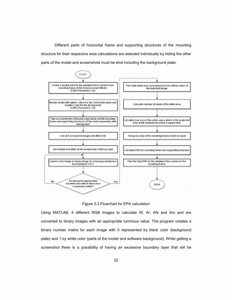
Different parts of horizontal frame and supporting structures of the mounting
structure for their respective area calculations are selected individually by hiding the other
parts of the model and screenshots must be shot including the background plate.
Figure 3.3 Flowchart for EPA calculation
Using MATLAB, 4 different RGB images to calculate Af, Ar, Afs and Ars and are
converted to binary images with an appropriate luminous value. The program creates a
binary number matrix for each image with 0 represented by black color (background
plate) and 1 by white color (parts of the model and software background). While getting a
screenshot there is a possibility of having an excessive boundary layer that will be
23
represented by white color which is trimmed off. Trimming off the boundaries is a big step
in the entire program. MATLAB identifies each column and row and tries to calculate the
sum of the first column. Then MATLAB will start to compare the sum of the first column
with the next column and it proceeds. If the sum of other columns is equal to that of the
first most one, that column will be deleted. This process stops when the sum of a
particular column is less than that of the first one. Now the process starts again from the
last column in the reverse way and stops until the sum of column is less than that of the
last column. The same procedure is followed for all the rows and thus the excessive
boundaries with value 1 are deleted.
The background plate’s area is called in as an input by MATLAB and pixel
number of all 4 images are counted and saved in the memory. Then, percentage white
pixels to whole image are obtained using MATLAB codes. Now, MATLAB multiplies the
percentage with the area of the background plate which was called in earlier which gives
us all the white region values. These white region areas represent the projected area of
flat, round parts of horizontal and supporting structures of the mounting structures. After
getting all the projected area, the MATLAB gets gross area dimensions as input. All
calculated areas and input gross area are then used in their respective formulae
mentioned above in chapter 2 to calculate the total EPA of the mounting structure with
windward direction acting along the azimuth’s normal face. The software tool gives an
alternative to calculate the projected area of an assembly instead of hand calculation
where we still have to check every single part’s detail to calculate their projected area
which takes more time, especially for mounting structures with lot of parts. This method is
also helpful to quickly calculate the projected area of faces in different angles to the
windward direction if needed.

24
3.3. Verification of the Method
The methodology of calculating EPA using image processing through MATLAB
tool was explained in detail in the section above. Though theoretically explained, the
method required verification for one of the mounting structure which is currently being
used in the market. To verify the method, we requested a cad model of an existing model
from CommScope Incorporation and they sent us one of their own models SF-QV 14-B.
The exact methodology is followed for the model and the EPA result of SF-QV 14-B
obtained from MATLAB is compared with the manufacturer’s value [5].
Figure 3.4 SF-QV 14-B mount structure [5]
Figure 3.5 SF-QV 14-B mount with background plate [18]

25
The binary images of the flat and round frame, supporting structures are also shown in
this chapter below.
Figure 3.6 Binary image of frame structure
Figure 3.7 Binary image of flat members of supporting structure [17]

26
Figure 3.8 Binary image of round members of supporting structure [17]
The EPA values of frame, supporting structures and the entire mounting structure after
substituting the projected areas calculated through MATLAB [17] in the standard
equations are shared below in the tables.
Table 3.1 Effective projected area [17]
EPAMN EPAFN EPAN
13.28 ft2 6.27 ft2 19.59 ft2
Table 3-2 MATLAB and manufacturer value comparison
EPAN (MATLAB) EPAN (CATALOG) [5] Error percentage
19.59 ft2 20.45 ft2 4.2 %
27
The results of SF-QV 14-B model [5] from CommScope Inc is calculated using image
processing through MATLAB programming tool and compared with the manufacturer
value. The calculated result of EPA is 19.59 ft2 and that of manufacturer’s is 20.45 ft2 [5].
Thus it is clearly understandable that there is only a 4.2 % difference between the values
and the difference is considered to be error percentage of the method used. Wind load is
measured by EPA multiplied with wind pressure and with this 4.2% difference in EPA will
have an impact in wind force calculation. Since EPA and wind force are linearly
dependent whatever change in percentage occurs in EPA will be the same in wind load
values. So based on the 5% allowable rule used in industries, it is safe to say that
anything below 5% is considerable for mounting structure models. Thus it shows that the
method is a good enough alternative to manual calculation. More over this method is
quick as it saves a lot of time and human error in calculation will also be reduced when
compared with manual calculation.
Though the results are acceptable, the error percentage can be improved to have
better set of EPA values close to manually calculated value. The error percentage can be
taken as one of the limitations of the method used in this project. As discussed earlier the
error percentage can be improved with better resolution and pixel density of the computer
screen used. The computer screen used in this case is a 23 inches Dell screen with a
resolution of 1920 x 1080. As MATLAB converts images to binary images and counts the
number of pixels for further are calculation, it is easy to improve results when we have
good resolution computer screens through which we snap screenshots of the structures
to be used for projected area calculation. Such high resolution screens like 27 inches HP
screen with 2560 x 1440 resolution, 24 or 32 inches NEC Multisync with 3840 x 2160 and
ACER 28 inches with 3840 x 2160 can be used to improve results.
28
Chapter 4
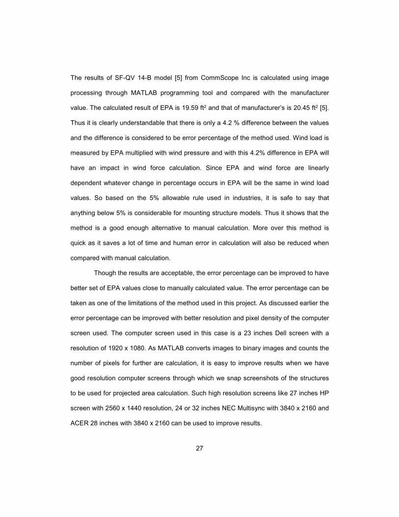
NEW ANTENNA MOUNTING STRUCTURE DESIGN
4.1. Mount CAD model
The new model is designed with the all basic requirements and not
compensating on any of the design parameters. The mounting structure consists of frame
and supporting structures. The number of parts of the frame structure is reduced by
having only one horizontal frame structure with plate structures supporting the vertical
pipes used to hold antenna and remote radio units. The reduction in assembly parts
reduces the EPA of the frame and also the weight of the whole mounting structure. The
horizontal frame does not exceed the limit of 14.5 ft and the antenna units are placed on
the frame equidistant to each other from one end to the other.
Figure 4.1 Mounting structures with vertical pipes [18]

29
The frame structure of the mount is connected to the tower through the
supporting structures. The use of rectangular plates is required to connect the horizontal
frame towards the supporting structures. In this model, we used four main supporting
structure pipes to form two different sets of V-frame type structures. They are fixed are at
two locations on the frame structure to form a perfect symmetrical body. This is to have a
model that is well supported from the tower to carry the dead weight and additional load.
Thus the entire model has reduced a lot of assembly models compared to the other
existing models. The V-frames are all connected to the tower using connecting plates that
can have additional plates in case if we need to increase the stand-off distance.
Currently, this model carries a stand-off distance of 42 inches which is within the design
limit.
Figure 4.2 Mounting structure with Antenna-Radio units [18]

30
The connection plates and vertical pipe connections used to connect antenna
units are all shown in the images below.
Figure 4.3 Frame and supporting structure connection plate [18]
Figure 4.4 Antenna vertical tube connection plate [18]

31
4.2. Material Data
Material selected for the mounting structure should always satisfy ASME
standards. Most of the mount structures are always some of the steel structures with
different grades. So, we go by the same selection with steel structures for our mount
model. All the steel structures must be galvanized with zinc to avoid rusting problems
after installation of the mounting structure. The material properties of all the material used
and assumed are provided in the tabular data below in this chapter 4.
Table 4.1 Material property data
Material Density
(lb ft-3)
Elastic
modulus
( psi)
Poisson’s
ratio
Yield
strength
(psi)
A36-steel 490.06 2.90E+07 0.26 36300
A500-
steel
490.06 2.90E+07 0.26 45687
Antenna-
material
1.6855 3.48E+07 0.3 1E+06
RRU-
material
1.2948 3.48E+07 0.3 1E+06
A36, A500 grade steels are selected because they are currently being used for
manufacturing mounting structures and they can also withstand self-weight and dead
load applied on them for the dimension used. Our main concern in this project is to
design and analyze only the mounting structure. Hence, we are assuming the material
properties of antenna and remote radio units used in here. The assumptions of yield

32
strength and Elastic modulus are so high compared to steel structures. The reason
behind the selection is that the antenna and radio units must not bend or show max
stresses for high wind loads. We are going to study only the mounting structures and
hence to avoid other stress concentration distraction we assume high strength materials
for antenna-radio units. While assuming the material property it is highly important to use
the density properly. As per design parameters, the antenna with 180 lbs and 2 radio
units with 60 lbs each should carry a combined load of 300 lbs dead weight. Thus the
densities are calculated with the given weight and are used in as material properties. The
other main steel material properties are used by referring MatWeb website [20] for this
thesis.
4.3. Finite Element Model
Finite element method is used to analyze the mounting structure modelled in
CREO parametric 3.0 by using ANSYS 15.0 simulation software. The simulation process
is carried out in ANSYS workbench which acts as a graphical unit interface. For this
model, we carry out static structural analysis and the work flow of the analysis used is
shown in the picture below.
Figure 4.5 Schematic diagram of structural analysis

33
4.3.1. Importing CAD model
All the required materials are included in the ANSYS workbench library through
engineering data. All the required properties like densities, isotropic coefficients, yield
strength and ultimate strength can be plugged in from the property chart shown on the
left side of the figure below. These materials can then be called into the solver while
analyzing easily.
Figure 4.6 Material library in ANSYS workbench 15.0 [19]
The CAD model with assembly parts designed is converted and saved as a
STEP file. The STEP file is then imported into ANSYS design modeler to start structural
analysis. It is always recommended to turn on the surface bodies, line bodies option in
design modeler to import all parts of the assemble model without losing anything. Then
generate the model and the whole assembly is created within design modeler. For this
assembly mounting structure model we have approximately around 490 parts which
includes all the steel tube, pipes, bolts, U-bolts, connection plates and reference tower
leg. If necessary the different parts can be color coded differently to differentiate them

34
and also naming them is an option that can be helpful while analyzing in the mechanical
solver. The imported model in ANSYS 15.0 [19]can be seen in the below image.
Figure 4.7 Imported geometry model
4.3.2. Contact analysis
After importing and generating the CAD model in ANSYS, it is moved to the
mechanical solver where the model is pre-processed to get structural results. When the
model is sent to the solver all the contacts between parts are all generated automatically
based on assembling of parts in CREO parametric [18]. Before going onto analyze it is
always good to check the contacts if there are any unnecessary contacts acting between
different parts. For this manual check, ANSYS provides us an option named contact

35
information where the program will run throughout all the contacts and produces a data
sheet that has the penetration, gap, type of contact, status and pin-ball radius for each
contact. Based on that it is easy to pre-check all the contacts and delete the unwanted
contacts. Color codes represented to inform the user that the contacts could be far open
or too close or proper. In our model all contact types are bonded and hence a linear type
problem. The initial contact information generated helped to delete excessive contacts
created and also helped increase pin ball radius for contacts those were open but had to
be bonded. By increasing pin ball radius based on the gap information it is easy to make
the bonded contact more active than being far open. Finally, checking all the contacts is
absolutely necessary so that the model would not have more gaps between parts which
will create peak stresses and mislead the analysis.
Figure 4.8 Initial contact information
4.3.3. Meshing the Model
Once the model is checked for contacts the next important step to carry out is to
mesh the model using different options. There are plenty of meshing methods available in
ANSYS 15.0. Each model has to be meshed based on its geometry and structure. There
are different types of elements while generating mesh for a body. Tetrahedral,
hexahedral (brick) and prism elements are the different types of mesh elements. Brick
elements are the best element to be used since it produces an even mesh over a body
part and also reduced the count of elements produced.

36
Some of the element pictures are shown below.
Figure 4.9 Tets, bricks, prism and pyramid mesh elements
While generating mesh for model, there are two strategies to be followed. Using global
meshing methods at first and then based on the model requirements local meshing
methods can be used.
Figure 4.10 Proximity and Curvature mesh method [19]

37
In this case, one of the advanced mesh method is used as a global method to
produce fine number of elements for the entire structure. Proximity and curvature is used
for the model because of the round structures and chamfered edges in it. Proximity and
curvature method specifically recognizes all the closely placed faces and curved
structures and meshes them with finer elements which cannot be achieved using other
global mesh methods. The element size gradually grows from 25inches to 0.125 inches
based on the size and shape of the structure. The growth rate for all the mesh elements
that grows from edges towards the whole body is 1.8 approximately.
Figure 4.11 Detailed view of the meshed mounting structure [19]
38
After globally meshing the model, a local mesh method named hex dominant is
used on parts which have larger surface to volume ratio. This particular method tries to
create better brick elements or hexahedral elements which will reduce the number of
element rather than having tetrahedral mesh elements more in number. The main
mounting frame structure is locally meshed with a face sizing which creates three
elements on its thickness. All the parts those have a stable body structure that is the
body doesn’t alter from source face to target face are considered as sweep-able bodies
and are meshed with brick elements easily. Other parts which are not sweep-able are all
meshed with tetra-hedral elements. Thus following all the above stated meshing
techniques, we finally generated the model with 6 million element count and 13 million
nodes approximately. Once meshing is done, all the contact information should be
regenerated because contacts depend on nodes too.
4.3.4. Boundary Conditions
After meshing the entire mounting structure, the model has to have all the
boundary conditions before solving the entire analysis. Boundary conditions are all based
on the project definition and design parameters. As discussed earlier, the mounting
structure has to carry its own weight and a dead load of 2000 lbs which includes antenna-
radio unit weight and human load who works up on towers to fix all those bolts. The
mounting structure should also withstand a wind load at a height 250 ft above ground
level and wind load values are determined using standard formulae and picked from
calculated data table shown in chapter 2. All the boundary conditions allotted for this
particular mounting structure is discussed in this section.
• The connection plates used to connect all those V-frame type supporting
structure to the tower leg are all fixed.

39
• Since the entire model is fixed at a height of 250 ft from ground level, standard
gravitational force acts on the whole structure. Thus, in this model a force of
32.174 ft/s2 acts on the negative Y direction.
• As the structure is exposed to wind, a pressure of 0.206 psi taken from the
previously calculated tabular data strikes against the mount in the direction
normal to the frame structure of the mount model. In this case, the 0.206 psi wind
pressure acts on the negative Z direction.
• Other important condition of the mount design is to withstand human load of 500
lbs and so the load is added to act on the weakest point of the whole model
which is one of the edge of the horizontal frame structure because it could
provide more stress on the entire model. So, in directional sense this 500 lbs
load acts towards negative Y direction.
Figure 4.12 Boundary conditions [19]

40
Chapter 5
RESULTS
5.1. Effective Projected Area results [17]
To calculate the EPA for the new mounting structure projected in windward
direction acting normal to the azimuth of the frame, the same image processing method
is used since it is verified that the method is good alternative. As per standard
calculations EPA for the mount structure is calculated separately for frames and
supporting structures.
5.1.1. Effective projected area of frame structures
As discussed in the earlier chapters, snap shots of just frame structures
projected onto the reference background plate are taken. Then they are called into
MATLAB to get binary images and calculate the projected area which is then substituted
in the standard equations to get effective projected area. Before taking snapshots the
frame structure which in here the only the horizontal frame is decomposed into two
sections based on the shape of the parts. Here, the horizontal frame has flat and round
members and projected area calculated separately. Finally the program gives the EPA of
the frame structure.
The EPAMN results and binary images are showed below which are calculated through
MATLAB codes.
Table 5.1 EPAMN Result
Af Ar EPAMN
2.9ft2 4.2ft2 9.9ft2

41
Figure 5.1 Binary image of flat members of frame structure
Figure 5.2 Binary image of round member of frame structure

42
5.1.2. Effective Projected Area of supporting structures
As we calculate the EPA for frame structure, supporting structures are also disintegrated
into two different sections based on the shape that is round and flat members. Projected
area is calculated for both flat and round members of the supporting structures and the
values are multiplied with their corresponding drag coefficient to calculate the EPA and
they are added up to calculate EPA for entire supporting structure. The results and binary
images are shown below.
Table 5.2 EPAFN Result
Afs Ars EPAFN
4ft2 4.7ft2 6.8ft2
Figure 5.3 Binary image of flat members of supporting structures

43
Figure 5.4 Binary image of round members of supporting structures
And, finally both effective projected areas of frame and supporting structures are
summed to calculate the overall EPA of the mounting structure projected in the windward
direction acting normal to the azimuth of the frame.
Table 5.3 EPAN Result
EPAMN EPAFN EPAN
9.9ft2 6.8ft2 16.7ft2
The EPAN calculated for mounting structure is about 16.7ft2 which does not exceed the
maximum limit that is 64ft2. Also the new mount has a lower EPA when compared the
currently used mounting structure by CommScope Inc. The results are better than most
of the mount structures and hence it is the first success for the model and it gave way to
go on work on finite element analysis.

44
5.2. Finite Element Analysis Results [19]
Finite element analysis is carried out for the mount model in ANSYS workbench
15.0 with all the boundary conditions we got from EIA/TIA 222 rev G standards. The
stress, deformation and strain results are analyzed and elaborately discussed in this
chapter.
5.2.1. Stress and Strain Results
After defining the material properties, contacts between parts and meshing the geometry,
we define the boundary conditions before starting to run the simulation. For this model
stress results were analyzed and since the materials used are all steel structures which
are ductile and also the mounting structure having multiaxial loadings, it is safe to
analyze the equivalent von-mises stress instead of normal and shear stresses
individually. Von-mises stress is nothing but a logical way to sum of all the directional
stresses. Von-mises stress results can be further compared to the yield strength to verify
whether the entire model satisfies von-mises stress criterion.
�� = ������^ �����^ ������^�
^1/2 ≥ �� 15
Where, σ1, σ2 and σ3 are principle stresses of the model on all three directions, σv
represents the von-mises stress and σy represents the yield strength. Von-mises criterion
can be stated as the model will fail when the von-mises stress exceeds the yield strength.
Figure 5.5 Von-Mises and maximum shear stress criterion [16]
45
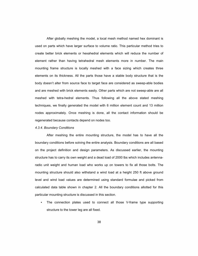
The stress results for the mounting structure is shown and discussed below.
Figure 5.6 Maximum von-mises stress point [19]
As shown in the figure 5-6 above the results are clear that most of the model does not
experience a stress beyond 2331.6 psi which are represented by dark blue color. Though
there are points where higher stress occurs and particularly in this image the max point is
not visible. For that, a zoomed version of the area of concern in different views is shown
below.
Figure 5.7 Detailed view of max stress point [19]

46
Figure 5.8 Detailed front view of the max stress point [19]
From the figures, it is clear that the max stress occurs at the junction of the
horizontal frame and the supporting structures where there will be a lot of tension and
compression force due to wind pressure and human load acting on different directions.
The max stress is around 21ksi on the horizontal frame but since the material used is
A500 the von-mises stress is lower than its yield strength which is 45ksi. The factor of
safety can be calculated for the model using the formula,
F.S. = σy/σv 16
Thus, safety factor of 2.2 is obtained for this model and so it can be said that the
mounting structure is mechanically stable for the loading conditions.
The strain results are also calculated as stress and equivalent strain points are
shown in the images below. As per hooke’s law, max strain points will occur at the same
stress points since the materials are ductile and have elastic properties.

47
Figure 5.9 Strain result [19]
Just like the maximum stress point, strain results are also not visible and hence the
zoomed views of the max strain points are shown below.
Figure 5.10 Detailed view of max-strain point on frame structure [19]

48
Figure 5.11 Detailed front view of max strain point on frame structure [19]
Results show that the max strain occurs at the same spot as the stress and the max
value is 7.4E-04 and lies within the yield range of the material used. Thus the model is
stable enough for all given load conditions.
5.2.2. Total Deformation Result
Figure 5.12 Total Deformation (True scale) [19]

49
The deflection results are analyzed for the model since there are multiple loads
and it is important to check these results. From the results it is clear that the maximum
deformation occurs at the vertical tubes holding all the weight of antenna-radio unit of 300
lbs on the side where human load acts. But the max deformation is way low and hence
will not affect the mounting structure when it is applied with a human load at the weakest
point of the entire frame structure. Also we have additional tiebacks connecting the outer
most vertical pipes towards the tower legs and they act as additional support to reduce
the deflection further. Thus the deformation results also show that the mounting structure
designed is perfectly stable.
In the true scale image of deformation 0.22in deflection is not clear enough for
the viewer to see and so the results effects are magnified by 66 times and now it is visible
where the 0.22in deflection occurs.
Figure 5.13 Magnified view of the deformation [19]

50
Chapter 6
Conclusion
The EPA along the windward face normal to the azimuth face of the mounting
structure has been successfully calculated using Image Processing through MATLAB
R2014a software which has not been done previously in the telecommunication field. The
calculated EPA 16.7 ft2 which compared to the other sample mounts used in the market
is much lesser. The minimized EPA helps to reduce the Wind load acting on the structure
and reduces the weight of the Mounting structure itself. One limitation of the method is
that a computer screen with a good resolution and a higher PPI should be considered so
that the pixels of the image are much higher and more accurate.
The max deformation and Stress results calculated are 0.22in and 21ksi respectively
which shows that the mount structure is stable and also the frame will have tie backs
extending from the tower legs which will further reduce the deflection and stress values
acting on the mounting structure. Validation for the simulated results can be done by
experimental analysis for the model by assembling the whole mounting structure and
then with the help of a wind tunnel results can be measured. The next analysis to be
carried out will be for the same model with high wind pressures to check its stability under
bad weather conditions and have a dynamic load analysis. Vibration analysis can also be
done for the mount but for that the vibration data for the towers is also required. The
Mounting structure analysis for transient load conditions can to be simulated as a future
work.

51
References
1. A Green Road. (2013,). Free energy wardenclyffe tower wireless energy
demonstration project, wireless communication through earth, rain making machine.
Retrieved from http://agreenroad.blogspot.com/2013/06/nikola-tesla-free-energy-
wardenclyffe.html
2. Goldsmith. A (2005). In cambridge university press (Ed.), Wireless
communicaion (pp. 237-240)
3. Jain. A (1989). Digital imale processing Prentice Hall.
4. Audio Engineering Society. (2002). The telefunken radio station at sayville, long
island. Retrieved
from http://www.aes.org/aeshc/docs/recording.technology.history/sayville.html
5. CommScope Incorporation. (2013). CommScope inc catalog (5th edition ed., )
6. Committees (Ed.). (2006). EIA/TIA 222 rev-G standard. Arlingotn: TIA standards and
Engineering publications.
7. Elcosh Company. (2011). Types of telecommunication towers. Retrieved
from http://www.elcosh.org/index.php
8. Engineers Garage. (2012). Image processing. Retrieved
from http://www.engineersgarage.com/articles/image-processing-tutorial-applications?
9. ENT Journal. (november 27, 2012, ). Nikola tesla and his discovery of wireless
technology. Retrieved from https://entjournal.wordpress.com/2012/11/27/nikola-tesla-
and-his-discovery-of-wireless-technology/
10. Fiber Optics Associations. (2015). Fibre optic cables. Retrieved
from http://www.thefoa.org/user/

52
11. Ishtiaq Muhammad. (2012). Manufacturing and erection of telecommunication
towers (B.E Mechanical Engineering).
12. R.G.a.R. Woods. (2006). Digital image processing (3rd Edition ed.) Prentice Hall.
13. Tower direct. (2-015). Selfsupporting towers. Retrieved
from http://towerdirect.net/used-190-self-supporting-towers/
14. Ruben Gregory Puthota. (2015). Next generation antenna mounts. International
Technical Conference and Exhibition on Packaging and Integration of Electronic and
Photonic Microsystems, San Francisco, CA. 1.
15. Nikola tesla and his vision. . (2012, sep 28). [Video/DVD] Youtube:
LaboratoryTesla.
16. efunda. (2015). Failure criteria for ductile materials. Retrieved
from http://www.efunda.com/formulae/solid_mechanics/failure_criteria/failure_criteria.c
fm
17. Mathworks. (2014). Matlab r2014a (8.3rd ed.)
18. PTC. (2014). Creo parametric 3.0 (3.0th ed.)
19. Canonsburg, P., U.S. (2015). ANSYS workbench (15.0th ed.)
20. MatWeb. (2015). Online material information. Retrieved
from http://www.matweb.com/

53
Biographical Information
Ruben Gregory is a Mechanical engineer graduate student at University of Texas
at Arlington who completed his studies in summer, 2015. He had a great opportunity to
work for couple of company projects with CommScope Incorporation and his area of
interest has always been design engineering and the thesis work speaks about the
interest. Ruben graduated from SKCET, India as an undergraduate in mechanical
engineering in 2011 during which did an internship for a year with BHEL, India a power
plant equipment manufacturing company. Ruben Gregory lives in Arlington, Texas, USA.
In future, Ruben would love to work for oil-based industry as a Design engineer and gain,
improve knowledge with industrial experiences.
Recommended