Clemson UniversityTigerPrints
All Theses Theses
12-2012
DESIGN AUTOMATION ANDOPTIMIZATION OF HONEYCOMBSTRUCTURES FOR MAXIMUM SOUNDTRANSMISSION LOSSRohan GalgalikarClemson University, [email protected]
Follow this and additional works at: https://tigerprints.clemson.edu/all_theses
Part of the Mechanical Engineering Commons
This Thesis is brought to you for free and open access by the Theses at TigerPrints. It has been accepted for inclusion in All Theses by an authorizedadministrator of TigerPrints. For more information, please contact [email protected].
Recommended CitationGalgalikar, Rohan, "DESIGN AUTOMATION AND OPTIMIZATION OF HONEYCOMB STRUCTURES FOR MAXIMUMSOUND TRANSMISSION LOSS" (2012). All Theses. 1514.https://tigerprints.clemson.edu/all_theses/1514

DESIGN AUTOMATION AND OPTIMIZATION OF HONEYCOMB STRUCTURES FOR MAXIMUM SOUND
TRANSMISSION LOSS
A Thesis Presented to
the Graduate School of Clemson University
In Partial Fulfillment of the Requirements for the Degree
Master of Science Mechanical Engineering
by Rohan Ram Galgalikar
December 2012
Accepted by: Dr. Lonny L. Thompson, Committee Chair
Dr. Joshua D. Summers Dr. Georges M. Fadel

ii
ABSTRACT
Cellular materials with macro effective properties defined by repeated meso-
structures are increasingly replacing conventional homogeneous materials due
to their high strength to weight ratio, and controllable effective mechanical
properties, such as negative Poisson‘s ratio and tailored orthotropic elastic
properties. Honeycomb structures are a well-known cellular material that has
been used extensively in aerospace and other industries where the premium on
the weight reduction with high-strength is required. Common applications of
honeycomb cellular structures are their use as the core material in sandwich
plates and plates between two face sheets. Honeycomb structures are built from
repetition of a common hexagonal unit cell tessellation defined by four
independent geometric parameters; the hexagonal unit cell side lengths, h, and l,
cell wall thickness, t and orientation of the angle between the cell walls . These
parameters can be controlled to achieve desirable effective properties.
Another important application of honeycomb sandwich structures is the ability
to adjust the unit cell geometric parameters to increase the Sound Transmission
Loss (STL); a metric for measurement of noise cancellation for acoustic waves
passing though the panel structure, while maintaining a low mass, and
controllable effective stiffness and strength properties. Previous research has
been limited to parametric studies exploring the effect of change in a single unit
cell parameter on the Sound Transmission Loss (STL). To obtain an optimal STL
result and to determine sensitivities, the present work presents a novel

iii
technique to control all four of the unit cell parameters while maintaining
constant overall dimensions and mass of the honeycomb sandwich plate. These
two constraints are necessary to ascertain that the high STL occurs only due to
the change in geometric properties of honeycomb unit cell, as the STL increases
with increase in mass and change in overall dimensions.
An optimization problem has been set-up with the design variables as hexagonal
interior angle, number of unit cells in the horizontal direction, and number of
unit cells in the vertical direction for a representative plate model with in-plane
acoustic pressure wave transmission analysis. These variables indirectly control
the other unit cell lengths and cell-wall thickness parameters while satisfying
the aforementioned constraints. All three of the design variables are restricted
to integers to ensure the resulting geometry is regular and manufacturable. The
STL response is optimized over a frequency range of 200-400 Hz, within a
typical resonance region of the frequency response function. The goal of the
optimization is to maximize the area under the STL curve over the frequency
range of interest, with constraints on fixed mass and overall plate dimensions.
The optimization process required a complete design automation workflow of
geometry creation based on changes in number of cells, constraints on overall
dimensions and mass, output results extraction, construction of response
surface to expedite the optimization using genetic algorithms. The process
involved a coupled structural-acoustic finite element model with direct steady-
state analysis and natural frequency extraction created and solved using the
commercial finite element software package ABAQUS. The model is used to

iv
obtain acoustic pressure values for calculation of the STL of the honeycomb
sandwich plate. Quadratic Timoshenko beam elements have been used to
discretize the thin-walled honeycomb cellular structures for increased accuracy
at higher frequencies. The elastic structure model is coupled with acoustic
elements by applying surface based tie-constraints to transfer normal plate
surface accelerations as input to calculate radiated sound pressure. The entire
process of finite element model creation and solution has been parameterized
and automated by extensive use of Python scripts directly interfaced with the
ABAQUS solver. A detailed workflow has been set-up in the optimization
package modeFRONTIER that generates the input variables using a genetic
algorithm, NSGA-II, controls the Python scripts to create and solve the finite
element Abaqus model, calls the Python scripts to extract results for post-
processing needed to generate the STL vs. Frequency plots and finally optimizes
the geometric unit cell parameters to maximize STL over a typical frequency
range, all while respecting constraints on overall dimensions and mass. The
frequency range from 200 Hz to 400 Hz was used to demonstrate the design
automation and optimization process developed. The same workflow can be
used to optimize STL for other frequency ranges.
To speed-up the optimization process, approximation functions have been
generated utilizing the Response Surface Methodology (RSM) in modeFRONTIER.
The Shepherd K-Nearest algorithm was found to be the most accurate of five
alternative RSM functions considered. It has been shown that interpolation with
this function accurately predicts the output with less than 1% error and

v
significantly speeds up the optimization process compared to a complete finite
element solution at each iteration.
Results of the optimization process show that although a single design with the
highest STL measure was found, in general, the designs with less than-25o ,
number of horizontal cells greater than 60 and the ratio of unit cell lengths
(h/l) greater than 1 also give relatively high STL values over the frequency range
studied. The designs with the highest STL measure show close to 70 %
improvement over the designs with the lowest measured STL. Design trends
have also been observed for the stiffness properties of honeycomb core. The
designs with highest value of STL have low *
11E and
*
12G in comparison to the
designs with the lowest STL. However the *
22E is high for designs with high STL
and low for designs with low STL.
To determine the most important design variables affecting STL results a
sensitivity analysis has been conducted using the Pareto-chart of standardized
effects. The results indicate that all the three design variables have a significant
impact on the output. The significance in the descending order is the number of
vertical cells, the number of horizontal cells and the unit cell wall orientation .
This result is noteworthy given that was the only design variable considered
for the parametric studies conducted previously.

vi
DEDICATION
This work is dedicated to my parents Mr. Ram Galgalikar and Mrs. Vibha
Galgalikar , my uncle Mr. Nitin Bendre and aunt Mrs. Charu Bendre for their
continual and unconditional love and support.

vii
ACKNOWLEDGEMENTS
First of all I would like to thank Dr. Thompson for his inputs and support
throughout the two years at graduate school as an advisor. His inputs have been
invaluable to this research. The inputs and support of my committee members
Dr. Summers and Dr. Fadel have helped me in this research as well.
I would also like to thank the modeFRONTIER customer support team for their
help with resolving the software issues.
I would also like to thank Clemson University as a whole for providing the
necessary resources and conducive atmosphere for my studies. Further I would
also like to thank the other professors from whom I learnt a lot through the
coursework.
Finally I would like to thank my roommates and close friends who helped me
through the highs and lows of the graduate school.

viii
TABLE OF CONTENTS
ABSTRACT .............................................................................................................................. ii
DEDICATION ......................................................................................................................... vi
ACKNOWLEDGEMENTS ...................................................................................................... vii
TABLE OF CONTENTS ....................................................................................................... viii
LIST OF TABLES ................................................................................................................... xii
LIST OF FIGURES ................................................................................................................. xv
Chapter 1 : INTRODUCTION .............................................................................................. 1
1.1 Sandwich Plates .......................................................................................................... 1
1.1.1 Sandwich plates with honeycomb core .......................................................... 2
1.2 Sandwich Plates in Structural Acoustics .............................................................. 4
1.2.1 Sound Transmission Loss (STL) ....................................................................... 4
1.2.2 Previous research in Structural Acoustics: ................................................... 9
1.3 Optimization and honeycombs in structural acoustics: ................................. 11
1.4 Motivation and Goals .............................................................................................. 13
1.5 Thesis objectives ...................................................................................................... 14
1.6 Thesis Overview ....................................................................................................... 15
Chapter 2 : OPTIMIZATION PROBLEM SET-UP ............................................................. 18
2.1 Honeycomb unit cell and related formulae ....................................................... 18
2.2 Optimization Problem............................................................................................. 21
2.2.1 Objective: ............................................................................................................ 21
2.2.2 Input variables: .................................................................................................. 21
2.2.3 Output variables:............................................................................................... 22
2.2.4 Derived variables: ............................................................................................. 23
2.2.5 Constraints: ........................................................................................................ 23
2.2.6 Constants: ........................................................................................................... 24
2.3 Calculations of the derived variables: ................................................................. 25

ix
2.4 Structural-Acoustic Model ..................................................................................... 26
2.4.1 Model ................................................................................................................... 26
2.4.2 Selection of representative frequency range .............................................. 27
2.4.3 Transmission and reflection of incident sound wave .............................. 28
2.4.4 Effect of angle of incidence on the sound transmission ......................... 29
2.4.5 Use of in-plane model of honeycomb instead of the
out-of-plane model ........................................................................................... 30
Chapter 3 : DESIGN AUTOMATION METHOD ............................................................... 33
3.1 Description of the modeFRONTIER Workflow: ................................................. 34
3.2 Detail description of the workflow: ..................................................................... 36
3.2.1 Calculating the input variables ...................................................................... 36
3.2.2 ABAQUS Model Creation and Solving ........................................................... 37
3.2.3 Post-processing ................................................................................................. 38
3.3 ABAQUS Model Set-up of the Honeycomb Sandwich Plate
and Python script ..................................................................................................... 40
3.3.1 Parts ..................................................................................................................... 40
3.3.2 Material properties: .......................................................................................... 40
3.3.3 Sections: .............................................................................................................. 41
3.3.4 Beam Orientation: ............................................................................................. 42
3.3.5 Step ...................................................................................................................... 43
3.3.6 Assembly............................................................................................................. 44
3.3.7 Mesh: .................................................................................................................... 45
3.3.8 Load:..................................................................................................................... 46
3.3.9 Boundary Conditions: ...................................................................................... 47
3.3.10 Postprocessing ................................................................................................ 48
3.3.11 Python script: .................................................................................................. 50
3.3.12 Output Python script: .................................................................................... 51
3.4 Challenges in integrating modeFRONTIER & ABAQUS: ................................... 52
3.4.1 Location of the output files generated by ABAQUS .................................. 52
3.4.2 Compatibility of the versions of the softwares ......................................... 52

x
3.5 Model Validation ...................................................................................................... 52
Chapter 4 : RESULTS OF DOE AND RSM ........................................................................ 56
4.1 Design of Experiments (DOE) ................................................................................ 56
4.1.1 Response Surface Methodology ..................................................................... 60
4.2 Generating RSM functions ..................................................................................... 64
4.2.1 Comparison of RSMs ........................................................................................ 65
4.3 Global Optimization using RSMs .......................................................................... 67
4.3.1 Comparison of optimal solutions RSMs: ..................................................... 69
4.4 Local Optimization Results using RSM ............................................................... 71
4.4.1 Verification of solutions near the optimum design for accuracy ......... 74
Chapter 5 : SENSITIVITY ANALYSIS AND DESIGN TRENDS ...................................... 76
5.1 Actual design: ........................................................................................................... 76
5.2 Correlation: ................................................................................................................ 77
5.3 Validation of RSM .................................................................................................... 79
Chapter 6 : ANALYSIS OF STL CURVES .......................................................................... 84
6.1 Comparison of the optimal design with a reference case .............................. 84
6.2 Natural Frequencies and mode shapes ............................................................... 87
6.2.1 The mode shapes of the mode numbers 15, 20 and 25: ......................... 89
6.2.2 The mode shapes corresponding to 16th, 17th, 18th
and 19th mode numbers: ................................................................................. 90
6.2.3 Natural Frequencies of the reference configuration................................. 93
6.3 Comparison of the STL curves .............................................................................. 95
Chapter 7 : CONCLUSIONS AND FUTURE WORK ....................................................... 100
7.1 Accomplishments: ................................................................................................. 100
7.2 Conclusions: ............................................................................................................ 101
7.3 Future work: ............................................................................................................ 103
REFERENCES ....................................................................................................................... 105
APPENDICES ....................................................................................................................... 109

xi
Appendix A : air_honeycomb_edit_input.py .......................................................... 109
Appendix B: output_air_honeycomb_edit.py ......................................................... 127
Appendix C: honeycomb.m ........................................................................................ 128
Appendix D: matlab_output.m .................................................................................. 129
Appendix F: output. Bat .............................................................................................. 129
Appendix G: DOE case-1 design table: ..................................................................... 129

xii
LIST OF TABLES
Table 1-1: Hierarchy of sandwich composte properties with cellular core ............ 3
Table 2-1: Upper and lower bounds on the design variables ................................... 22
Table 3-1: Material Properties of Aluminum ................................................................ 40
Table 3-2: Material Properties of Air .............................................................................. 41
Table 3-3: Section properties for core and facesheets ............................................... 41
Table 3-4 : Standard sandwich plate model used for validation ............................. 53
Table 4-1: Results of DOE-1 conducted with the workflow-1
having ABAQUS model in it. ......................................................................... 56
Table 4-2: Sample designs from DOE-1 conducted with workflow-1
with ABAQUS model in it. ............................................................................. 57
Table 4-3: Design with the highest STL measure obtained in DOE-1
conducted with workflow-1 having ABAQUS model in it. ..................... 59
Table 4-4: Comparison of RSM functions with performance measures
given in modeFRONTIER ............................................................................... 67
Table 4-5: Results of optimization conducted with the workflow-2,
having RSM node, for four RSM functions ................................................ 69
Table 4-6: Honeycomb unit cell parameters for the optimal designs
obtained from the RSMs ................................................................................ 70
Table 4-7: Truncated Design Space ................................................................................ 72
Table 4-8: Original design space ..................................................................................... 72
Table 4-9: Optimization results in the truncated design space............................... 73

xiii
Table 4-10: Optimal design in the truncated design space obtained
by an optimization using workflow-2 and
Shepherd K-Nearest RSM function............................................................ 73
Table 4-11: Designs evaluated near the optimal design for verification
of the optimal solution ............................................................................... 75
Table 5-1: Correlation coefficients ................................................................................. 77
Table 5-2: Results of DOE using Shepherd K-Nearest RSM with workflow-2 ....... 79
Table 5-3: Designs with the least value of STL in terms of area under
the curve in the descending order from DOE-1 ...................................... 81
Table 5-4: Designs with the least value of STL in terms of area under
the curve in the descending order from DOE-1 ...................................... 83
Table 6-1: Unit cell parameters for reference and optimal designs ....................... 84
Table 6-2: Comparison of the optimal design and reference design ..................... 86
Table 6-3: Natural Frequencies of the honeycomb plate of the optimal
design ................................................................................................................ 88
Table 6-4: Natural frequencies of the honeycomb plate of the
reference configuration ................................................................................ 93
Table 6-5: STL in terms of area under the curve and RMS values for
the 3 designs with the highest and 3 with the lowest values
for 200-400 Hz range .................................................................................... 96
Table 6-6: Honeycomb unit cell parameters correspoding to the designs
with the highest and lowest values of STL measure............................... 96

xiv
Table 6-7: Effective stiffness properties of honeycomb cores
corresponding to designs with the highest and lowest
values of STL measure .................................................................................... 98

xv
LIST OF FIGURES
Figure 1-1: Plate with core sandwiched between two thin skin layers ..................... 1
Figure 1-2: Hierarchy of properties of sandwich structures with cellular core ..... 2
Figure 1-3: STL characteristics of a typical wall partition [18] .................................. 5
Figure 2-1: Honeycomb unit cell left: regular right: auxetic ................................... 18
Figure 2-2: Sandwich plate with same overall dimensions but with a
diffrent core .................................................................................................... 22
Figure 2-3: Auxetic honeycomb unit cell left: constraint satisfied ....................... 23
Figure 2-4: Calculations of derived variables ............................................................... 25
Figure 2-5: Model set-up ................................................................................................... 26
Figure 2-6: Transmission and reflection of incident sound wave ........................... 28
Figure 2-7: In-plane configuration of honeycomb sandwich plate.......................... 31
Figure 2-8 : Out-of-plane configuration of honeycomb sandwich plate ................ 31
Figure 3-1 : A brief overview of the modeFRONTIER workflow
with ABAQUS ................................................................................................ 34
Figure 3-2: modeFRONTIER workflow-1 with ABAQUS for DOE and
Optimization .................................................................................................. 35
Figure 3-3: Orientation ...................................................................................................... 42
Figure 3-4: Partitioning the horizontal edge of Air .................................................... 44
Figure 3-5: Mesh for Air .................................................................................................... 46
Figure 3-6: Load................................................................................................................... 47
Figure 3-7: Boundary Conditions .................................................................................... 47

xvi
Figure 3-8 : Sandwich plate for the reference configuration .................................... 53
Figure 3-9: STL vs. Frequency plot for reference configuration ............................. 54
Figure 3-10: STL vs. Frequency plot for the refernce configuration
obtained using workflow-1 ...................................................................... 54
Figure 4-1:Honeycomb sandwich plate for the design with the
highest STL obtained from DOE-1 conducted with workflow-1
having ABAQUS model in it. ........................................................................ 59
Figure 4-2: Overview of the process used for generating and
using RSM functions. .................................................................................... 60
Figure 4-3: Process overview of the workflow-2 with RSM function
used for predicting the STL results .......................................................... 61
Figure 4-4: Workflow-2 with the RSM node used to predict the
STL results instead of solving the ABAQUS based
Structural-acoustics finite element model .............................................. 62
Figure 4-5 :Comparison of workflow-1 with ABAQUS and workflow-2
with RSM node ............................................................................................... 63
Figure 4-6: RSM distance plot for Shepherd K-Nearest Algorithm .......................... 65
Figure 4-7: RSM distance plot Neural Networks algorithm ....................................... 66
Figure 5-1: Results of Sensitivity analysis on DOE-1 .................................................. 76
Figure 5-2: Correlation of design variables to output variabale .............................. 78
Figure 5-3: Sensitivity analysis on the results of DOE conducted
using the Shepherd K-Nearest RSM with workflow-2 ........................... 79
Figure 6-1: Honeycomb sandwich plate for the reference configuration .............. 84

xvii
Figure 6-2 :Comparison of the STL vs. Frequency plot for the
optimal and reference configuration ...................................................... 85
Figure 6-3 : Sandwich plate left: reference configuration
right: optimal configuration ..................................................................... 85
Figure 6-4: Mode 15 freq: 235.56 Hz .............................................................................. 89
Figure 6-5: Mode 20 Freq: 289.88 Hz ............................................................................. 89
Figure 6-6: Mode 25 freq: 348.34 Hz .............................................................................. 89
Figure 6-7: Mode 16 freq: 248.31 .................................................................................... 90
Figure 6-8: Mode 17 freq: 262.13 Hz .............................................................................. 90
Figure 6-9: Mode 18 freq: 262.71 Hz .............................................................................. 90
Figure 6-10: Mode 19 freq: 278.72 Hz ........................................................................... 91
Figure 6-11: Acoustic region for the fleuxural mode-15. .......................................... 91
Figure 6-12: Acoustic region for Dilatational mode-16 ............................................. 92
Figure 6-13: Mode 3 freq: 208.22 Hz .............................................................................. 94
Figure 6-14: Mode 4 freq: 286.29 .................................................................................... 94
Figure 6-15: Mode 5 freq: 365.18 .................................................................................... 94
Figure 6-16: Comparison of the STL curves of the three designs
with the highest STL and the three with the lowest STL
for constant mass of sandwich plate .................................................... 95
Figure 0-1: Unit cell line and vertex numbering ........................................................ 126

1
CHAPTER 1 : INTRODUCTION
Cellular materials occur commonly in nature, e.g. wood, cork, sponge and corral
etc. Manmade cellular materials like foam are popularly used today. Their
popularity is primarily attributed to the capability of modification of properties
to accommodate a wide range of design requirements. Design engineers do not
have this flexibility with conventional materials like homogeneous materials [1].
Applications of cellular materials include light weight structures, energy
absorbing applications and packaging applications[2],[3]. Cellular materials
usually form the core of the sandwich plates between the two skins or face
sheets.
1.1 Sandwich Plates
Figure 1-1: Plate with core sandwiched between two thin skin layers
Sandwich plates are made up of two face sheets or skins and a core between
them [4]. Figure 1-1 shows of a typical sandwich plate. The core increases the
area moment of inertia of the composite. Hence it has high strength to weight

2
ratio [5], [1]. Various materials like foam, trusses and honeycomb structures
have been used as core for the sandwich plates [6],[7], [8].
1.1.1 Sandwich plates with honeycomb core
Sandwich plates made up of honeycomb core have high out-of-plane stiffness
and low in-plane stiffness[9]. Honeycomb structures are constructed from two
dimensional prismatic cellular material of periodic meso-structures this process
of repetition is also referred to as tessellation. Meso-structures in this context
refer to the repetitive hexagonal unit cell of the honeycomb. The properties of
sandwich plates can be described by the hierarchy shown Figure 1-2 [10],[11].
Figure 1-2: Hierarchy of properties of sandwich structures with cellular core
Macro
Meta
Meso
Micro

3
Table 1-1: Hierarchy of sandwich composte properties with cellular core
Hierarchy Definition
Micro Properties of the base material such as steel or aluminum
Meso Geometric properties of honeycomb unit cell: h, l, t,
Meta Effective mechanical properties of the honeycomb core
Macro Overall behavior of composite sandwich plate including skins.
By changing the meso-properties of the honeycomb unit cell, the meta-
properties of the honeycomb core can be changed. This in-turn changes the
macro properties of the sandwich plate thus giving flexibility to the designer to
customize the design as per specific requirements [12]. For example,
honeycomb structures have been designed for high shear deformation [13].
Honeycombs have also been designed to have high shear strength and shear
strain simultaneously [9]. It has been established that honeycomb structures
have high crush strength [14][2]. The use of honeycomb structures in heat-
exchanger applications has also been shown to be advantageous [15].
Honeycomb structures with negative cell wall angles known as auxetic or re-
entrant honeycomb have different properties than honeycombs with positive
angles. Auxetic honeycombs have a negative effective Poisson‘s ratio and hence
offer advantages over the regular honeycombs in applications such as smart
fasteners under tensile loads, seals and gaskets, and in shock absorption [16].

4
Honeycomb structures have also been shown to be effective in structural
acoustics applications for sound absorption and noise canceling properties
[10][17][18]. The following section gives an overview of use of sandwich plates
and honeycomb in structural acoustics.
1.2 Sandwich Plates in Structural Acoustics
1.2.1 Sound Transmission Loss (STL)
In structural acoustics two concepts related to reduction of sound levels are, (a)
sound absorption, (b) sound insulation [19]. Sound absorption is defined as
conversion of sound energy into heat energy, whereas sound insulation is
defined as the ―blocking‖ of incident sound wave [19]. Both of these
phenomenons are frequency dependent. Sound absorption coefficient
defined as the ratio of the energy absorbed to the energy incident, and
sound transmission coefficient defined as the ratio of the transmitted to the
incident sound energyare used as metrics for measurement of these
phenomenon.
Sound absorption is helpful for sound reduction within a confined space.
However for sound reduction between two spaces the phenomenon of sound
insulation with reduced transmission is important [19]. This research focuses on
the concept of sound insulation with sound transmission through finite sized
sandwich plate structures.

5
A zero value of implies that no sound energy is transmitted whereas value of
one implies that all the incident sound energy is transmitted, with no reflection
or absorption of energy. Sound Transmission loss (STL) is defined as the log of
the inverse of the sound transmission coefficient [19]:
10
1STL log
(1.1)
The unit of STL is decibel (dB). Figure 1-3 shows the variation of STL with
frequency for sound transmission through a typical wall partition [19].
Figure 1-3: STL characteristics of a typical wall partition [18]
The frequency response of the STL function can been divided into four different
regions, (a) Stiffness, (b) Resonance, (c) Mass, and (d) coincidence region
according to the behavior of the partition. The STL can be increased in the low

6
frequency region by increasing the stiffness of the partition [20]. However the
stiffness region is limited to low frequencies and ends at the first natural
frequency of the wall partition [20].
In the second, mid-frequency region known as resonance region, the natural
frequencies of the partition control the STL characteristics. In this region the
honeycomb structures have been used advantageously to achieve higher STL by
changing their meso properties [10] [17].
In the mass region, the behavior of the STL through the partition does not
depend on the elastic properties or stiffness of the partition, and is governed
only by the plate mass. In this mass region, the STL is referred to the ―mass
law‖, and is defined by the relative mass of the plate and surrounding air
mediums, speed of sound, angle of incidence, and frequency [21]
10
0 0
cosSTL log 1
2
s
c
(1.2)
In the above,
sMass per unit area of the partition. (Kg/m
2 )
frequency of the incident sound wave (Hz)
angle of incidence (degrees)
Density of the surrounding air medium (Kg/m3)
c0 : speed of sound in the surrounding air medium (m/s)

7
As the angle of incidence increases from normal incidence at
to its upper
limit 90o
the STL decreases for a given frequency. In the actual physical
environment incident sound waves do not have a single angle of incidence. They
are modeled with field incidence in which the angle of incidence is averaged
from
to
with all the sound waves having equal intensity [21]. The slope
of this STL line in the mass region is 6 dB/octave, meaning that for doubling of
frequency the STL increases by 6 dB [21]. In the mass region, the effective elastic
and stiffness properties of the honeycomb meta-structure will not affect STL, as
in this region, the increase in STL for a particular frequency occurs only with
increase in mass of the partition.
In the fourth, high-frequency region of the graph is the coincidence region. In
this region a major dip in the STL curve occurs. This dip corresponds to the
critical frequency of the elastic partition given by
2
0
2
sc
cf
B
(1.3)
In the above, B is the bending stiffness of the partition (N/m2), and f
c is the
critical frequency (Hz)
Coincidence occurs when the speed of the wave travelling through the plate
equals the speed of sound c0 in the surrounding medium [19],[21].
8
From the Figure 1-3 it can be noticed that the dips in STL can be reduced by
adding damping to the partition [19] ,[22].
For finite plates, resonance occurs when the frequency of the incident sound
wave equals the natural frequency of vibration of the plate [21]. Resonance is of
two types: Flexural vibration modes and dilatational modes. Both these modes
cause a dip in the STL typically at low frequencies. The phenomenon of
resonance is absent in infinite plates as there is no reflection of sound waves
from the end of plates[21].
For the plates with finite size coincidence occurs when both the frequency of
the incident sound wave matches a resonance frequency (either flexural or
dilatational) and the speed of the incident sound wave matches the wave
velocity in the plate (either flexural or dilatational) [21]. Coincidence occurs
typically at high frequencies. For plates of infinite size, as resonance does not
exist, coincidence occurs when the speed of the wave travelling through the
plate equals the speed of sound in the surrounding medium [21],[23]. At
coincidence the impedance of the plate becomes zero resulting in high sound
transmission or low STL [23]. The effects of coincidence on sound transmission
through plates have been investigated in [24],[25],[26],[22],[27],[21].

9
1.2.2 Previous research in Structural Acoustics:
Kurtze et.al [27] demonstrated, in their seminal paper, that the sandwich plates
have better acoustical performance compared with single wall. They designed
plates having a very high ratio of static to dynamic stiffness. With these
characteristics plates have sufficient stiffness to support static loads as well as
high sound transmission loss [28]. They also explored the effects of flexural
coincidence on the STL characteristics of sandwich plates.
Ford et.al [23] further extended this work to investigate the effects of
dilatational coincidence on STL characteristics. They related the dilatational
critical frequency, the minimum frequency at which dilatational coincidence
occurs, to the thickness and the stiffness of the core. They also optimized these
two core properties for a polyurethane core plate to obtain both the flexural and
dilatational critical frequencies above 4000 Hz. Also for this plate the low order
flexural modes occurred below 100 Hz. Thus the STL characteristics of the plate
followed the mass law in the 100-4000 Hz frequency range [25]. In this work
the Rayleigh-Ritz minimum energy principle was used to obtain the analytical
model to predict the resonance frequencies[25]. However this model had some
drawbacks [24][27]. Smolenski and Krokosky used the strain energy principle to
derive a better analytical model to predict the natural frequencies of the plate
[27]. They also demonstrated that the flexural modes are not sensitive to the
changes in the core thickness and Poisson‘s ratio, whereas the dilatational
modes are highly sensitive to these changes [27].

10
The analytical models presented in the above mentioned papers were limited to
calculating the natural frequencies of the plates. Dym and Lang presented the
first analytical model to calculated the sound transmission loss of the sandwich
plates[24].They made further improvements to the analytical model of
Smolenski and Krokosky by using the plate theory. Using this improved model
Dym and Lang validated the findings of Kurtze et al. and Krokosky et al. [24].
In a further study Dym and Lang established that feasibility of optimization for
maximizing the sound transmission loss of a sandwich plate [29]. Their
objective was to maximize the average sound transmission loss over the
frequency range of 1000-4000 Hz. They formulated four optimization problems:
sandwich optimization, core optimization, skin optimization and thickness
optimization. For a proper comparison with the reference case the plate surface
mass was restricted to the highest value of 0.90 g/cm2
[29]. This ensured that
the optimal sandwich plate would have the same total mass as that of the
reference plate. They concluded that for practical purposes the optimal
sandwich plate will have high bending stiffness and lower bending coincidence
frequency in comparison with the reference case [29].
Shanbag et al. studied sound transmission through sandwich plates made of
viscoelastic cores [22]. They studied the effects of change in the core shear
parameter, loss factor and geometric factor on the sound transmission loss
characteristics. Their findings were: the core shear parameter had the most
significant impact on the STL, high value of core loss factor with suitable values
of core shear parameter and geometric parameter result in high STL. Also the

11
advantages of using the viscoelastic core were found to be shift of the
coincidence frequency to a higher value and a high value of STL per se at the
coincidence frequency [22].
Moore et al. derived analytical expressions for the STL of sandwich plates made
up of orthotropic cores [23]. They also proposed a unique design of sandwich
plate for high STL. As per this design the plate exhibits a double wall or
dilatational coincidence frequency lower than the frequency range of interest as
opposed to a higher dilatational frequency in the earlier designs. The anti-
symmetric or bending coincidence frequency of the plate is higher than the
interested frequency range [23].
Lin et al. proved a very interesting and simplifying property for sound
transmission through sandwich plates[30]. Their study showed that the STL
characteristics of parallel plates separated by periodic structures can be
approximated very accurately by considering vacuum instead of air in the cavity
[30].
1.3 Optimization and honeycombs in structural acoustics:
Thamburaj et.al conducted an optimization study to maximize the sound
transmission of a sandwich plate [18]. Keeping the mass of the sandwich plate
constant and constraining the stiffness of the plate two different optimization
studies, core optimization and thickness optimization, were conducted. Their
findings confirmed that anisotropic cores have better STL characteristics
compared to isotropic cores. The results of the thickness optimization suggest

12
that thin skin on the incident side and thick skin on the transmitted side
produce better STL characteristics[18]. However this study had some limitations.
Only three discreet values of frequency were considered. The optimal designs
for each of these frequencies were different[18] . In practice an optimal design
of a sandwich beam should have good STL characteristics for a wide range of
frequencies.
Denli et al. have also conducted optimization study to maximize the STL of
sandwich plates [31]. The displacements of the nodes of the beam were taken as
design variables for this optimization study. The fundamental frequency was
constrained to a minimum value to maintain the stiffness of the structure [31].
However this study had the following limitations: the number of design
parameters was extremely high: 120 and 258. The optimal geometry obtained
was highly irregular. For the second study the optimal geometry has changing
thickness [31]. Manufacturing these optimal geometries could be uneconomical.
Franco et al. have also conducted optimization study on sandwich plates for
maximizing the STL [32]. They considered various configurations for the
optimization of random core, homogenous core and truss like core to conclude
that truss like core, by changing its cross-section area, could be optimized to
achieve better sound transmission characteristics in terms of minimum spatial
mean square velocity. Another important finding from this study was that the
use of gradient based methods for structural-acoustic optimization is not
suitable as the algorithm gets trapped in local minima [32]. One limitation of
this study is that the design space has not been fully explored since the design

13
variables were the facesheet thicknesses and core densities. The number of
spatial points used for measurement of the velocity is less and hence the results
are coarse.
Ruzzene explored the effects of using honeycomb structures in the sandwich
plates on the STL characteristics [17]. Ruzzene used a spectral formulation to
model the acoustic and structural response of the plate. The findings show that
the use of honeycomb structures in the core of the plate gives better STL
characteristics compared to the 2D truss like structures[33]. Ruzzene tried four
different configurations of honeycomb unit cells and showed that the negative
angle or ―re-entrant‖ honeycombs have better STL characteristics than the ones
with positive angles [17].
This work was further extended by Griese, who studied the effect of change in
angle between the cell walls of the honeycomb structures on the STL of the plate
[10]. Griese changed the angle from -45o to + 45o with a fixed number of unit
cells in the beam and demonstrated that plates with negative angled honeycomb
had better STL characteristics compared to the positive angled honeycomb for
the same mass of the plate [10].
1.4 Motivation and Goals
The effective properties of sandwich plate are also dependent on vertical cell
height h, slant height l and cell wall thickness t of the honeycomb unit cell apart
from angle between the cell walls However in Griese‘s study was the only
design parameter to be changed freely to study the effect of its change on the

14
STL characteristics of the sandwich plate. Thus the entire design space was not
explored as the other unit cell parameters vertical cell height h, slant height l
and cell wall thickness t were governed by the fixed number of unit cells present
in the sandwich beam with fixed dimensions. Also the results of optimization
study of Denli and Sun had limitations such as high number of design variables,
highly irregular resulting geometries. Further none of these studies presented
design automation for a complete parameterization or optimization of sandwich
honeycomb plates with the four independent unit cell geometric variables. With
this motivation the objective of this thesis is as follows.
1.5 Thesis objectives
1. Set up an optimization problem to study the effect of change in all the
design parameters vertical cell height h, slant height l and cell wall
thickness t and angle between the cell walls on the STL characteristics
of the sandwich plate. Find the optimal design that will maximize the
STL.
2. Study the effect and importance of each design variable on the final
output.
3. Maintain the total mass of all the sandwich plates constant. It has been
established that with increasing mass the STL loss of the plate increases
[10]. Hence to have a fair comparison of the all the models it is necessary
to maintain their mass constant.
15
4. Maintain the overall dimensions of the sandwich plate constant so that
changes in the stiffness and mass of the sandwich plate are only
controlled by the changes in unit cell geometry of the honeycomb core.
5. Automate the entire optimization process
6. Generate an approximation function (RSM function) to make the
optimization process computationally less expensive.
7. Demonstrate the effectiveness of the developed optimization process
with a typical frequency range within the resonance region of the
sandwich honeycomb plate.
1.6 Thesis Overview
Chapter 1:
The chapter 1 introduces the concept of cellular materials and sandwich plates.
An important distinction between the sound absorption and sound insulation
has been discussed. The concept of Sound Transmission Loss (STL) and related
formulae are presented. The STL characteristics of sandwich plates with the
advantages of using honeycomb cores have been explained. Literature review
section presents the prior research done in the field. Finally the motivation and
thesis objective are explained.
Chapter 2:
The chapter 2 begins with the definition of honeycomb unit cell and formulae
for geometrical and material properties of honeycomb cores. The next section
discusses the optimization problem defining the design variables, derived

16
variables, constraints, constant parameters, objective function and the output
variables. The calculations of the derived variables have been explained in the
next section. The last section of this chapter explains the structural acoustic
model set up used for this study. The phenomenon of reflection of the incident
sound wave and the effect of angle of incidence on the sound transmission has
been explained. The rationale for selecting the in-plane configuration of
honeycomb instead of the out-of-plane configuration has been provided.
Chapter 3:
In this chapter a detailed explanation of the modeFRONTIER workflow used to
automate and solve the optimization problem has been provided. Further the
details of the structural-acoustic finite element ABAQUS model have been
discussed. The calculations for STL have been explained. Finally the python
scripts generated to automate the ABAQUS model creation and solving have
been discussed.
Chapter 4:
Chapter 4 presents the results of optimization. The need for meta-modeling and
the process used for generating the approximation functions has been
explained. Further the selection of the approximation function with the least
error and the results of optimization using this function have been presented.
Chapter 5:
This chapter presents the results of sensitivity analysis and correlation. These
results demonstrate the significance of the design variables in terms of the

17
impact on the output variable. Further the designs trends observed from the
optimization results have been discussed.
Chapter 6 and 7:
In the chapter 6 the STL vs. frequency curves have been analyzed for the design
with the highest area under the curve (auc). This has been compared with a
reference case. The reasons for the dip in the STL have been investigated. Finally
a comparative study of the designs with the highest and lowest auc is
presented. The geometry of these designs is also discussed.
The chapter 7 presents the conclusions of the study and the future work that
can be done to extend this study. Finally in the appendix section the python
scripts, MATLAB codes and the designs obtained from DOE have been
presented.

18
CHAPTER 2 : OPTIMIZATION PROBLEM SET-UP
In this chapter the concept of honeycomb unit cell has been introduced. This is
followed by the optimization problem, calculations of derived variables the
structural-acoustic model set-up with its details.
2.1 Honeycomb unit cell and related formulae
Figure 2-1: Honeycomb unit cell left: regular right: auxetic
The honeycomb unit cell as shown in Figure 2-1 has been previously used by
other researchers [34],[11],[10].
2 cosxL l (2.1)
2( sin )yL h l (2.2)
19
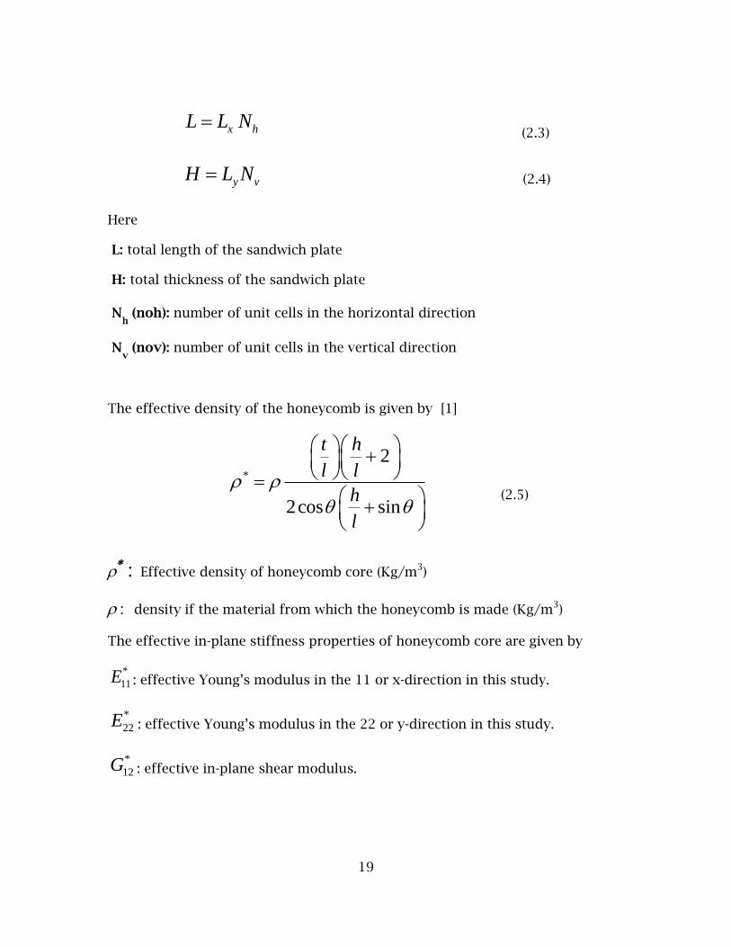
x hL L N (2.3)
y vH L N
(2.4)
Here
L: total length of the sandwich plate
H: total thickness of the sandwich plate
Nh (noh): number of unit cells in the horizontal direction
Nv (nov): number of unit cells in the vertical direction
The effective density of the honeycomb is given by [1]
*
2
2cos sin
t h
l l
h
l
(2.5)
Effective density of honeycomb core (Kg/m
3)
density if the material from which the honeycomb is made (Kg/m3)
The effective in-plane stiffness properties of honeycomb core are given by
*
11E : effective Young‘s modulus in the 11 or x-direction in this study.
*
22E : effective Young‘s modulus in the 22 or y-direction in this study.
*
12G : effective in-plane shear modulus.
20
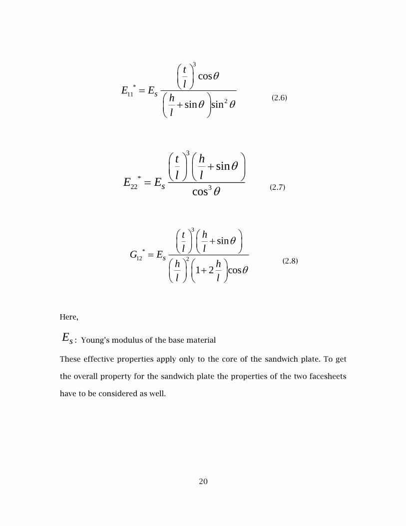
3
*
112
cos
sin sins
t
lE E
h
l
(2.6)
3
*
22 3
sin
coss
t h
l lE E
(2.7)
3
*
12 2
sin
1 2 cos
s
t h
l lG E
h h
l l
(2.8)
Here,
sE : Young‘s modulus of the base material
These effective properties apply only to the core of the sandwich plate. To get
the overall property for the sandwich plate the properties of the two facesheets
have to be considered as well.
21
The advantage of the effective property is that the honeycomb core can be
replaced with a homogenous plate having that property[1]. This simplifies the
calculations. In this particular study the mass of the core is calculated by the
product of the effective density and the total volume occupied by the plate as
shown in equation (2.9)
Mass of core, *M L H D (2.9)
where
D : the depth of the core (D = 1 m for this study)
2.2 Optimization Problem
2.2.1 Objective:
Maximize the Sound Transmission Loss (STL) of the honeycomb sandwich plate
by maximizing the area under the curve (auc) of the STL vs. Frequency graph for
the chosen frequency range.
2.2.2 Input variables:
Table 2-1 lists out the design variables chosen for this study. The upper
and lower limits of these variables have been shown to define the design space
for the optimization problem. All the design variables have been constrained to
be integers.

22
Table 2-1: Upper and lower bounds on the design variables
Variable Lower limit Upper limit
-45o 45o
Nh
20 100
Nv 1 10
Figure 2-2 shows the effect of change in number of unit cells on the core on the
sandwich plate while maintaining the overall dimensions same.
Figure 2-2: Sandwich plate with same overall dimensions but with a diffrent core
2.2.3 Output variables:
The output variable for the optimization problem is the area under the STL vs.
Frequency plot (auc).
This output variable has been chosen to obtain a single representative value of
the STL performance of the sandwich plate for the chosen frequency range.

23
2.2.4 Derived variables:
Vertical unit cell height h, slant height of the unit cell l, and the angle between
the cell walls
2.2.5 Constraints:
1. h > 2 mm (for )
2. | 2 sin |h l
(for )
3. Nh(noh), N
v (nov) and are integers
Figure 2-3: Auxetic honeycomb unit cell left: constraint satisfied
right: constraint violated
The first constraint is a manufacturability constraint setting the lower limit on h
for ease of manufacturing [35]. The second constraint is a geometrical
constraint. If | 2 sin |h l
for < 0o
then the unit cell (Figure 2-1) will not be
a feasible geometry [35]. Figure 2-3 shows the two auxetic honeycomb unit cells
that satisfy and violate the 2nd constraint. The integer limits on the design
variables ensure that the resulting geometry from the optimization process is
regular and feasible. Additionally the integer constraint on restricts the
design possibilities to a real and finite number.

24
2.2.6 Constants:
1. 𝞺* = 270 Kg/m3 [10] (effective density of the core)
2. 𝞺 = 2700 Kg/ m3 ( Mass density of Aluminum)
3. L = 2 m, H = 8.66 cm
The total mass of the sandwich plate is maintained constant so that the changes
in the STL can be attributed only to the change in the unit cell properties of
honeycomb, as the STL increases with the increasing mass [10].
The overall dimensions of the plate are maintained constant to avoid changes in
the natural frequency of the plate due to change in dimensions which in turn
would affect the STL.
The particular values of effective density of the core and the overall dimensions
of the sandwich plate are chosen from [10] to have base model for validation of
the results obtained in this study.
Total mass (MT) of the sandwich plate is the addition of the masses of core and
the facesheets.
* 2T fM L H D Lt D
= 46.764 + 27 = 73.764 Kg
tf : thickness of the facesheet and is maintained constant at 2.5 mm. As the base
material (Aluminum) is constant and the other dimensions remain unchanged
the mass of the facesheets remains constant.

25
The mass of the core also remains constant as per the calculations shown in the
section 2.3. The value of and Nh govern the value of l. Further the value h is
defined by Nv and l. Finally as the effective density and hence the mass of the
core has to be maintained constant, t is calculated from the effective density
formula. Thus the total mass of the plate is maintained constant at 73.764 Kg.
2.3 Calculations of the derived variables:
Known: Nh
(noh), Nv (nov), L, H,
Unknown: Lx, L
y, h, l, t
Figure 2-4: Calculations of derived variables
Given: Nh, N
v, L, H,
26
2.4 Structural-Acoustic Model
2.4.1 Model
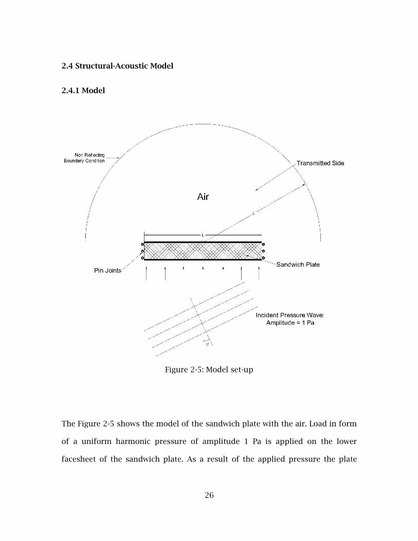
Figure 2-5: Model set-up
The Figure 2-5 shows the model of the sandwich plate with the air. Load in form
of a uniform harmonic pressure of amplitude 1 Pa is applied on the lower
facesheet of the sandwich plate. As a result of the applied pressure the plate

27
vibrates and radiates sound on the transmitted side. The radius of the semi-
circular air is same as the length of the sandwich plate L. Although the air has
been shown as a semi-circle it has been actually modeled with the non-reflecting
boundary condition on the semi-circular edge so that the transmitted sound
waves travel to infinity.
The angle of incidence of the applied pressure is 0o. This is also known as the
normal incidence[21]. In the gaps of the honeycomb core of the sandwich plate
it is assumed that vacuum is present to simply the calculations of STL [30].
2.4.2 Selection of representative frequency range
For the optimization problem a representative frequency range of 200-400 Hz
has been selected. As shown in Figure 1-3 the frequency range from
approximately 1-100 Hz is occupied by the stiffness region which is not relevant
to the current study. Further the dilatational modes of plate vibration occur
around 500 Hz causing unusual dips in the STL [10]. In order to accurately
capture the nature of these dips the frequency range should either be biased
towards the natural frequencies of the sandwich plate or a very high number of
frequency points with a linear range are required. The first method requires
solving the structural-acoustic model twice, once for natural frequency
extraction and then for the STL calculation, which is computationally very
expensive and time consuming. Automating this entire process presents further
challenges. To use the second method the frequency range has to be limited to
accurately capture the nature of STL plot. Thus to limit the complexity of the
problem the frequency range of 200-400Hz with a linear range and 100 points

28
has been selected to represent the typical resonance region for the sandwich
plate.
2.4.3 Transmission and reflection of incident sound wave
Figure 2-6: Transmission and reflection of incident sound wave
Interaction of sound waves travelling in a homogenous medium with another
medium is characterized by one of the three phenomenon: total reflection, total
transmission or partial reflection and partial transmission. This behavior is
governed by the speed of sound in both the mediums, density of the mediums
and the angle of incidence of the sound wave.

29
2
1 2
2trans
inc
p Z
p Z Z
(2.10)
2 1
2 1
ref
inc
p Z Z
p Z Z
(2.11)
The equation(2.10) and equation (2.11)specify the ratio of transmitted and
reflected pressure in terms of the characteristic impedance of the medium[21].
Here
pref
: reflected pressure amplitude (N/m2)
pinc
: incident pressure amplitude (N/m2)
ptrans
: transmitted pressure amplitude (N/m2)
Z1: characteristic impedance of medium 1.
Z2: characteristic impedance of medium 2.
2.4.4 Effect of angle of incidence on the sound transmission
For the case of c2 > c
1 (c
1 and c
2: speed of sound transmission in the respective
medium) there is limiting angle beyond which all the incident sound waves are
totally reflected[21]. For 0 < L , (is the angle of incidence and L
is the
limiting angle of incidence) the sound waves are transmitted into the other
medium[21].

30
1 11
2
sinL
c
c
(2.12)
All the formulae shown above apply to homogenous mediums only. The speed
of propagation of sound in aluminum is 5150 m/s[21]. Speed of sound in air is
343 m/s. Thus using equation (2.12) L = 3.81
o for air-aluminum interface.
However this result cannot be directly used for this study as the sandwich plate
is not a homogenous medium.
As the angle of incidence increases, for the same frequency, the STL of the beam
decreases[21]. However incident sound field with a single value of angle of
incidence is not observed in practice. Incident sound waves having equal
average intensity in all the directions is a better model of the actual
phenomenon. The angle of incidence is averaged from 0o to 78
o and model is
known as diffuse field[21].
2.4.5 Use of in-plane model of honeycomb instead of the out-of-plane model
Two types of sandwich plates can be created using the honeycombs are core:
out-of-plane and in-plane model. These configurations have been shown in
Figure 2-7 and Figure 2-8 respectively. These configurations are so identified
due the direction of the applied loads on their face sheets. For the in-plane
configuration the load on the face sheet of the sandwich plate is in the plane of
the honeycomb (in the y-direction as per Figure 2-7), whereas for the out-of-
plane configuration the applied load is perpendicular to the plane of the
honeycomb (in the z-direction as per Figure 2-8).

31
Figure 2-7: In-plane configuration of honeycomb sandwich plate
Figure 2-8 : Out-of-plane configuration of honeycomb sandwich plate
For structural acoustic applications where low sound transmission or high STL
is desirable the in-plane configuration has been shown to have better
performance over the out-plane configuration [23]. The primary reason for the
in-plane configuration having better STL characteristics is attributed to its low
in-plane stiffness that results in the ―double wall resonance‖ occurring at low
frequencies and low shear stiffness of the core that results in the coincidence
due to the flexural or anti-symmetric modes occurring at high frequencies [23].
The double wall resonance occurs when ― the mass of the face sheets in

32
resonance against the stiffness of the core‖ [23]. Thus in the frequency range of
interest generally 500-2000 Hz the STL does not degrade.

33
CHAPTER 3 : DESIGN AUTOMATION METHOD
An automated design workflow has been set-up to solve the optimization
problem by integrating ABAQUS 6.9.2, the commercial finite element package,
and modeFRONTIER 4.3.0, the commercial optimization software package.
Figure 3-1 shows a brief overview of this workflow using the ABAQUS model.
Figure 3-2 shows the actual workflow set-up in modeFRONTIER 4.3.0. This
workflow-1 can be used to run a Design of Experiments (DOE) as well as a full
optimization problem. Later another workflow-2 will be introduced which is
used to expedite the optimization process by predicting the outputs using the
mathematical approximation functions.
The design variables and the derived variables are generated in modeFRONTIER
as per the calculations shown in the Figure 2-4 . These input variables are then
used to generate the structural-acoustics coupled finite element ABAQUS model
using the Python script.

34
3.1 Description of the modeFRONTIER Workflow:
Figure 3-1 : A brief overview of the modeFRONTIER workflow with ABAQUS
process input
(DOE or optimization algorithm)
Data input
, Nv, Nh
calculations of derived variables and implementing constraints
using MATLAB
derived variables
h, l, t
ABAQUS model creation and solving with Python script
Postprocessing of ODB file with a Python script to calculate STL for
each frequency
plotting the STL vs. Frequency , calculating the area under the curve
of the plot with MATLAB and maximizing it

35
Figure 3-2: modeFRONTIER workflow-1 with ABAQUS for DOE and Optimization

36
3.2 Detail description of the workflow:
3.2.1 Calculating the input variables
, and are the input variable nodes containing the respective
variables. The upper and lower bounds on these variables are set while
configuring the nodes in modeFRONTIER. To implement the integer constraint
on these three variables the value of step is set as one in the node configuration.
This workflow has two MATLAB nodes: and .
The Matlab-69 node contains the honeycomb.m file which has to code to
calculate the derived variables (Figure 2-4). The Matlab-90 node contains the
output_air_honeycomb_edit.py file that contains the code for post-processing
calculations.
At the Matlab-69 node the design constraints are implemented by using
conditional variable at the process output connection.
All the application nodes in modeFRONTIER have two types of input and output
connectors: process connector and data connector. To implement the
constraints the output condition for the process output connector of the

37
Matlab-69 is specified by the variable x in honeycomb.m file. If the design is
infeasible value of x is zero and the process flow is terminated at node.
This results in the beginning of the next iteration. However in case of a feasible
design value of x is one and the process proceeds to the next node .
3.2.2 ABAQUS Model Creation and Solving
The next step in the process is the honeycomb sandwich plate creation and
solving in ABAQUS. All the variables namely angle, Nh, N
v, h, l, t are input to the
Python script
. This node contains a code ―air_honeycomb_edit_input.py‖
written in Python language which creates and solves the honeycomb sandwich
plate model. The code has been attached in the appendix.
The DOS batch script ―input.bat‖ in the node runs the ABAQUS
model. The file has been attached in the appendix.

38
The Job-1.odb file generated by ABAQUS is transferred to the next step using the
transfer file node .
3.2.3 Post-processing
There is a separate python script for post-processing of the outputs. The
―output_air_honeycomb_edit.py‖ script is contained in the node.
This script reads the output variables from the Job-1.odb file and does the post-
processing calculations on them. First the value of POR (acoustic pressure) for
each node in the nodeset (containing the nodes of air at the interface of air and
the top facesheet of the honeycomb sandwich plate) for all the frames (each
frame corresponds to a separate frequency) is read. The root mean square
(RMS) value of the POR for all the nodes is calculated for each individual frame
of the output. This further gives us the STL at a given frequency. These
calculations are explained in detail later. The node contains the
―output.bat‖ file that runs the output_air_honeycomb_edit.py file.

39
Further the values of STL calculated for the each frame are written to the
―abaqus.rpt‖ file contained in the node. From this file the two
vectors X (containing the values of frequency)and Y
(containing the values of STL ) are read. The MATLAB script ―matlab_output.m‖
(contained in the Matlab-90 nde) plots these vectors and calculates the STL in
terms of area under of the curve auc.
The output variable auc is contained in the node and the
objective of maximizing it is specified by the objective node .
The DOE and the Optimization algorithm are contained in the scheduler nodes
and respectively. These nodes are connected to
the process input connector of the Matlab-69 node.
For all the DOEs in this study the Uniform Latin Hypercube (ULH) has been used,
as this algorithm produces designs that are well scattered in the design space.
The optimization done this study uses the NSGA-II (Non-dominated Sorting
Genetic Algorithm-II) as it is robust[36].

40
3.3 ABAQUS Model Set-up of the Honeycomb Sandwich Plate and Python
script
3.3.1 Parts
Three parts are created initially.
1. Core
2. Facesheet
3. Air
Core: the core is modeled as 2D wire. First a single unit cell is created using the
given dimensions: h, l, t and . The entire core is then created by tessellation.
The linear pattern command is used to replicate the unit cell in the horizontal
and vertical directions.
Facesheet: This is modeled as 2D wireframe with length of 2m. In the assembly
module two instances of this part are created: one for the top of the core and
other for the bottom.
Air: Air is modeled as a 2D shell. Air is a semi-circle with radius 2m.
3.3.2 Material properties:
Aluminum is used as the material for the core and the facesheet. The material
properties of Aluminum as are follows
Table 3-1: Material Properties of Aluminum
Mass density Youngs’ modulus Poisson’s ratio
2700 Kg/m3 71.9E9 GPa 0.3

41
The material properties for air are shown in Table 3-2:
Table 3-2: Material Properties of Air
Mass density Bulk modulus
1.2 Kg/m3 141179.0 Pa
3.3.3 Sections:
Beam sections are assigned to the core and the facesheets. Two separate beam
sections are created for the sandwich plate: beamsection (for the core) and the
facesheet_beamsection (for the facesheets)
Their section properties are as shown in Table 3-3 :
Table 3-3: Section properties for core and facesheets
Beam section a
(m)
b
(mm)
Beamsection 1 t
Facesheet_beamsection 1 2.5
‗a’ is the out-of-plane thickness of the beam and it is set as 1m. This is same for
both the core as well as the facesheets. ‗b‘ is the in-plane thickness of the beam
and it has a constant value of 2.5 mm for the facesheets. The value of ‗b‘ for the
core changes to maintain a constant mass.

42
A solid homogenous section is created for the air.
3.3.4 Beam Orientation:
Beam orientations have to be assigned to the parts using the beam elements. In
this model the core and the face-sheets are meshed using the beam elements. In
2D models the default beam orientation is applied and it cannot be changed.
While assigning the beam orientation the direction of the ‗a‘ dimension of the
beam cross section has to be specified. In this model it corresponds to the
negative ‗z‘ direction. Hence ‗a‘ is the out-of-plane thickness. The Figure 3-3
shows the beam orientations assigned to the core.
Figure 3-3: Orientation
The red arrows in the figure indicate the direction of the tangent. Tangent
indicates the axial direction of the beam [37]. The plane of the beam cross
section is perpendicular to the tangent. The direction of a i.e. n1..
direction of b
i.e. n2
and tangent form a right handed triplet : 1 2 tangentn n .

43
Thus ‗b‘ is becomes the in-plane thickness.
3.3.5 Step
A SteadyStateDirectStep is created with a frequency ranging from 200 Hz to
400Hz with 100 points and linear scale. These three parameters: frequency
range, scale and number of points are important to accurately capture the dips
in STL.
One method to capture all the dips in the STL is to bias the points towards the
natural frequencies of the plate , as the dips correspond to the natural
frequencies [10]. However this method involves initial natural frequency
extraction making the model computationally expensive to solve. Automating
the process presents further difficulties.
Thus, for simplification purposes the frequency range was chosen as stated
earlier without compromising on the accuracy of the results. The frequency
range 1-100 Hz (approximately), which is the stiffness controlled region, is not
of interest in this study. Hence it is neglected. In the frequency range above 500
Hz the dilatational modes occur and cause unusual dips in the STL. Hence this
region is neglected as well.
Furthermore to ensure that all the dips of STL in the range 200-400 Hz are
captured 100 points have been used with a linear scale.

44
3.3.6 Assembly
To keep air, core and both the facehsheets together while vibrating surface-
based tie constraints are used. For creating tie constraints master and slave
surface have to be defined. The face-sheets are chosen as the master surface
and the vertices of the core, to which face-sheets are tied, are chosen as the
slave surface.
The air and the top face sheet are also tied together using the tie-constraint. The
lower edge of the air is partitioned (highlighted in red) as shown in the Figure
3-4
Figure 3-4: Partitioning the horizontal edge of Air
Only the partitioned part of the air vibrates with the sandwich plate meaning
that the load is applied only on that part. The other two parts are load free.
45
This partitioned part of the air and the top facesheet are tied together. Top
surface of the facesheet is the master and the lower surface of the edge of the
air is the slave surface.
3.3.7 Mesh:
The honeycomb core and the facesheets are meshed using the Timoshenko d
are used. These elements capture the transverse shear deformation and can be
used for the beams that have the cross-sectional dimensions up to 1/8 of the
axial dimensions [37]. This is specifically advantageous over the Euler-Bernoulli
beam elements in which the maximum allowed ratio of the cross-sectional to the
axial dimensions is 1/15 which is much lower than that of Timoshenko beam
elements [37]. Thus using the B22 elements is advantageous when value of h
and l is low.
However it should be noted that even if the out-of-plane dimension ‗a‘ is 1 m in
this model, it does not affect the results as this is a 2D model.
The mesh for the air is not uniform. It is biased to have more elements near the
air-honeycomb plate interface to capture the variation in the output variable
accurately near the interface, as high variation is expected in this region.
AC2D3, which is a 3 node 2D acoustic triangle, element is used to mesh air [37].
The Figure 3-5 shows the mesh of the air.

46
Figure 3-5: Mesh for Air
3.3.8 Load:
A time harmonic uniform pressure is applied on the lower facesheet of the
honeycomb sandwich plate. The amplitude of this pressure is 1Pa. this load is
perpendicular to the surface of the facesheet. Thus the angle of incidence is 0o
.Hence this is a forced vibration problem. The Figure 3-6 shows the application
of the load. The load is highlighted in red in the figure

47
Figure 3-6: Load
3.3.9 Boundary Conditions:
Both the sides of the honeycomb sandwich plate have been pinned i.e. the ‗x‘
and ‗y‘ translations are restricted to zero. The rotation is not restricted.
Figure 3-7: Boundary Conditions

48
The Figure 3-7 shows the boundary condition on one side of the plate. Similarly
the other side of the plate also has pinned boundary conditions. These
boundary conditions let the sandwich plate freely vibrate about the ‗z‘ axis.
3.3.10 Postprocessing
After the model has been solved by the ABAQUS an ―.odb‖ file is created, which
contains the outputs. The output required for calculating the STL is POR i.e.
acoustic pressure (N/m2). The POR is requested as a history output for nodeset
that consists of nodes on the air at the interface of air and sandwich beam. The
history output is specified so that the value of POR for each frame can be read
separately. Each frame corresponds to a different frequency. In this case
hundred frames have been requested as specified in section 3.3.5. The following
calculations are done for all the hundred frames to calculate the corresponding
values of STL.
1020log i
t
pSTL
p
(3.1)
Here
pi: RMS (Root Mean Square) value of pressure on the incident side (N/m
2).
pt: RMS (Root Mean Square) value of pressure on the transmitted side (N/m
2).
STL : Sound transmission loss measured (dB)

49
2 2 2
1 2 n
i
p p pp
n
(3.2)
Here p1, p
2,… p
n are the values of acoustic pressure of individual nodes on the
incident side. The value of acoustic pressure at all these nodes is 1 Pa. n is the
number of nodes: n = 101 on the incident side.
Acoustic pressure is a complex number and the magnitude of this complex
number is calculated.
Hence pi = 1 Pa
2 2 2
1 2 nt
p p pp
n
(3.3)
Similarly in the equation (3.3) p1, p
2, … p
n are the values of acoustic pressure of
individual nodes on the transmitted side. n is the number of nodes the values
of which is 101.
Then using the equation (3.1) STL is calculated for one frame of frequency. This
procedure is repeated for all the frames. The values of STL and frequency are
reported in ―.rpt‖ file. Further the STL vs. Frequency plot is generated by
MATLAB and its area under the curve, auc is calculated as shown in equation
(3.4) by evaluating the integral from a frequency of 200-400 Hz.

50
2
1
400
200
( )
f
f
auc STL f df
(3.4)
These calculations are implemented by a command ―trapz‖ in MATLAB.
3.3.11 Python script:
All the steps required to create a honeycomb sandwich plate, as shown in
sections 3.3.1 to 3.3.9, are implemented by a code written in Python language.
This code automates the entire process. An exhaustive list of commands
required to write the code is available in the ―Scripting Reference Manual‖ of
ABAQUS documentation [37]. The script takes h, l, t, Nh and N
v as inputs and
generates the honeycomb sandwich plate and solves it. The script
‗air_honeycomb_edit_input.py‘ has been attached in the appendix.
When a model is created in ABAQUS it generates a code that replicates the entire
process of model creation [38]. These commands are stored in a ‗.jnl‘ file
created in the running directory of ABAQUS. By changing the extension of the
‗.jnl‘ to ‗.py‘ a python script can be generated [37][38]. However this script has
commands that are specific to that model. For the purpose of this study the
python script was modified and parameterized.
The post processing part (section 3.3.10) is done by another Python script
―output_air_honeycomb_edit.py‖ attached to appendix. The code in this script
replicates the procedure shown in section 3.3.10.

51
3.3.12 Output Python script:
Calculations of STL can be done in the same python script that creates and
solves the model. However that script must wait for the model to be solved and
the ‗.odb‘ file to be generated. This can be accomplished using the
‗waitForCompletion(..)‘ command[37] . This command makes the script wait for
the results of the model and the commands that follow it are executed after the
ABAQUS has finished the solution.
However a problem is encountered when this script is implemented in
modeFRONTIER. Once ABAQUS has finished solving the model a ‗Job is done‘
message is generated. However the script has not been totally implemented at
this point. The STL calculations are done after this point. modeFRONTIER
workflow moves to the next process/node as soon it encounters the ‗Job is
done‘ message. This creates an error in the workflow.
Hence a separate python script that reads the ‗.odb‘ file and does the STL
calculations has to be used.
The modeFRONTIER workflow moves to the next node/process when the ‗job is
done‘ message, that is generated by the ABAQUS once the model has been
solved, is encountered. Hence that part of the script which is implemented after
ABAQUS has finished solving the job is not implemented and the following error
message is generated ―Is job done?.

52
3.4 Challenges in integrating modeFRONTIER & ABAQUS:
The important points to note when integrating the two softwares are:
3.4.1 Location of the output files generated by ABAQUS
By default ABAQUS generates the output files i.e the ―.odb‖ and ―.rpt‖ files in
the ―C:\Temp‖ folder of the machine [37]. However for modeFRONTIER to able
to read and process these files they must be saved to its running directory
which is different than ―C:\Temp‖. Hence the python script
air_honeycomb_edit_input.py has to be altered to accommodate these changes.
In the line no. 715 of this python script
mdb.jobs['Job-1']._Message(ODB_FILE, {'phase': BATCHPRE_PHASE,
'file': '.\\Job-1.odb', 'jobName': 'Job-1'})
the location of the ―.odb‖ file has been specified as '.\\Job-1.odb' instead of
'C:\Temp\Job-1.odb' so that the ―.odb‖ file is written to the running directory
of the modeFRONTIER.
3.4.2 Compatibility of the versions of the softwares
modeFRONTIER 4.3.0 is compatible with ABAQUS 6.9.x and lower versions [36].
For this study modeFRONTIER 4.3.0 is used with ABAQUS 6.9.2.
3.5 Model Validation
The STL results of a standard reference model were compared with that of the
same model from the Griese‘s study [10]. This model of the sandwich plate has

53
the parameters as shown in Table 3-4. Figure 3-8 shows the sandwich plate for
the reference configuration.
Table 3-4 : Standard sandwich plate model used for validation
Figure 3-8 : Sandwich plate for the reference configuration
Figure 3-9 shows the STL vs. Frequency graph for the sandwich plate with the
parameters shown in Table 3-4 from Griese‘s study [10]. The frequency range
used in Griese‘s study is 1-1000 Hz. Hence for validation purposes the
frequency range in the SteadyStateDirect step in ABAQUS was specified as 1-
1000Hz with a linear range and 100 points. However it should be noted that in
the later part of this study the frequency range has been reduced to 200-400 Hz
with the same number of points and linear range to have a higher accuracy of
the STL plot. The figure 3-10 shows the STL vs. Frequency plot obtained for
Reference
sandwich
plate
Nh N
v
h
(mm)
l
(mm)
t
(mm)
30 40 1 28.87 28.87 2.5

54
this study using the workflow-1 shown in Figure 3-2. The plot has been
generated by the workflow itself, thus helps to validate the entire design
automation model presented in this study.
Figure 3-9: STL vs. Frequency plot for reference configuration [10]
Figure 3-10: STL vs. Frequency plot for the refernce configuration obtained
using workflow-1
The plots shown in figure 3-9 and figure 3-10 agree very well with each-other
and thus validate the automated design procedure presented in this study. The
minor differences in these figures can be attributed to the fact that in Griese‘s
100 200 300 400 500 600 700 800 900 10000
10
20
30
40
50
60
70
80
90
100
Frequency (Hz)
ST
L (
db)

55
study a natural frequency extraction procedure was conducted prior to the
SteadyStateDynamic step that solves the structural-acoustic model. These
natural frequencies were later used to bias the frequency points to obtain a
smooth curve and capture the dips in the STL accurately. However for the study
presented here the natural frequency extraction procedure has not been
conducted prior to solving the structural-acoustic model, to avoid over-
complication of the modeFRONTIER workflow-1. However 100 frequency points
with the linear range validates the method used in this study. Further this range
is reduced to 200-400Hz keeping the number of frequency points same for
higher accuracy of the STL results.

56
CHAPTER 4 : RESULTS OF DOE AND RSM
4.1 Design of Experiments (DOE)
A design of experiments (DOE) was conducted using the Uniform Latin
Hypercube (ULH) algorithm with 500 designs. Workflow-1 shown in Figure 3-2
was used for this DOE. The ULH is suggested by the modeFRONTIER
documentation when a well scattered sample of designs is needed. This DOE is
referred to as DOE-1 hereafter.
The results of DOE are as shown in Table 4-1.
Table 4-1: Results of DOE-1 conducted with the workflow-1 having ABAQUS
model in it.
Total Designs 500
Feasible designs 274
Average run time per design 9.78 minutes
Total run time 44h:40m:12s
Note: All the computations reported in this study were run on machine with:
Processor: Intel® CoreTM2 Duo CPU T6500 @ 2.1 GHz. Installed memory (RAM):
3 GB

57
The Table 4-2 shows a sample of the results obtained in the DOE-1. A complete
table is provided in the appendix.
Table 4-2: Sample designs from DOE-1 conducted with workflow-1 with ABAQUS
model in it.
Design
ID Category
Nh Nv h
(mm)
l
(mm)
t
(mm) auc
11 ULH 0 81 8 5.41 12.34 0.444 5074.7
12 ULH -21 100 9 8.65 10.71 0.320 8598.6
13 ULH -31 73 5 16.89 15.98 0.486 8638.1
14 ULH -9 49 7 9.41 20.66 0.498 8253.5
15 ULH -35 64 8 16.35 19.07 0.310 NF
16 ULH -27 67 4 18.43 16.75 0.622 8578.3
17 ULH 17 47 3 7.92 22.24 1.17 7021.1
18 ULH 9 55 4 7.94 18.40 0.879 7917.4
19 ULH 3 74 3 13.72 13.53 0.956 7938.9
20 ULH 32 45 7 -7.7 26.20 0.615 NF
21 ULH -23 22 3 33.72 49.38 0.990 NF
NF implies that the design is not feasible. The designs 15, 20 and 21 are
infeasible as they do not satisfy the constraints ,which has been explained
below.

58
Design 15: as angle () < 0o
the constraint to be satisfied is
| 2 sin |h l
here h = 0.016353m and | 2 sin |l 0.02188m. Thus the constraint is
violated and the design fails.
Design 20: as angle () > 0o
the constraint to be satisfied is
h > 2mm. However the value of h = -0.0077m. Thus the constraint is violated
and the design fails.
Design 21: as angle () < 0o
the constraint to be satisfied is
| 2 sin |h l
here h = 0.033728 and | 2 sin |l 0.03858 m. Thus the constraint is violated
and the design fails.
In DOE-1 the design with the highest STL measured in terms of area under the
curve for the frequency range of 200-400 Hz is shown in the Table 4-3.

59
Table 4-3: Design with the highest STL measure obtained in DOE-1 conducted
with workflow-1 having ABAQUS model in it.
Design
ID Category
Nh Nv h
(mm)
l
(mm)
t
(mm) auc
67 ULH -39 68 3 26.34 18.92 0.661 8700
The geometry of the sandwich plate constructed with honeycomb unit cell as
described by the parameters shown in Table 4-3 has been shown in the Figure
4-1. The entire sandwich plate has not been shown for purpose of clarity. It can
be noticed that the core has 3 honeycomb unit cells with negative angles, known
as auxetic honeycombs (Figure 2-1), in the vertical direction. Similarly in the
horizontal direction 68 honeycomb unit cells are present, although not shown in
the figure.
Figure 4-1: Honeycomb sandwich plate for the design with the highest STL
obtained from DOE-1 conducted with workflow-1 having ABAQUS model in it.

60
4.1.1 Response Surface Methodology
It can be noticed from the results of DOE-1, shown in Table 4-1, that running
large number of iterations using the work-flow-1, shown in Figure 3-2 that has
the ABAQUS finite element model in it ,is computationally expensive. The
average run time for one design is around 10 minutes. Also large amount of
data, around 94GB mostly consisting of large ODB files from ABAQUS output, is
generated. Hence it is difficult to run an optimization problem using workflow-
1. Typically to obtain an optimized solution using a genetic algorithm the more
than one thousand designs have to be evaluated, which would be very time
consuming using the workflow-1. Hence the meta-modeling technique available
in modeFRONTIER has been used to generate mathematical approximation
function, also known as Response Surface Methodology (RSM) functions, that
predict the results faster than solving the ABAQUS based finite element model
shown in workflow-1.
The Figure 4-2 shows the overview of the process used in this study for
generating and using RSM functions.
Figure 4-2: Overview of the process used for generating and using RSM
functions.
DOE Generate
RSMs
Select the
best RSM
Optimization using the best RSM

61
The meta-modeling technique involves generating Response Surface
Methodology (RSM) functions, which are mathematical functions that predict or
approximate the output variable for the given inputs [36].
Figure 4-3: Process overview of the workflow-2 with RSM function used for
predicting the STL results
process input
(DOE or optimization algorithm)
Data input
, Nv, Nh
calculations of derived variables and implementing constraints using MATLAB
derived variables
h, l, t
RSM node
to predict the output
output: auc
and maxizing it

62
Figure 4-4: Workflow-2 with the RSM node used to predict the STL results
instead of solving the ABAQUS based Structural-acoustics finite element model
The process shown in the Figure 4-3 is similar to the one shown in Figure 3-1.
The calculation of derived variables is exactly same in both the processes. Figure
4-5 shows a comparison of the two workflows. In both the workflows
constraints are enforced similarly. However the part of the process that follows
the calculation of derived variables is different for the two workflows. The
process of ABAQUS model creation using the Python script, post processing of
ODB file for calculating the STL and plotting the STL vs. Frequency graph, has
been replaced by a single RSM node shown in Figure 4-4. This node
predicts the output variable using the mathematical approximation function.

63
The node contains an ―.rsm‖ file which has the mathematical function in it. The
file is not readable hence the mathematical function cannot be seen explicitly.
These functions make the entire simulation extremely fast thus making it
possible to run large number of iterations to get optimal results. To create an
RSM function a training data set, that is well-scattered in the design space, must
be provided. The design data of DOE-1, which is a well-scattered data set, is
used to train the RSM functions.
Figure 4-5 : Comparison of workflow-1 with ABAQUS and workflow-2 with RSM
node

64
4.2 Generating RSM functions
The 274 feasible designs from the DOE-1 are used to train and create the RSM
functions. The data wizard option available in modeFRONTIER has been used to
generate the RSM functions. The unit cell angle (Angle), number of unit cells in
the horizontal direction Nh (noh), number of unit cells in the vertical direction
Nv (nov), unit cell vertical height h, unit cell slant height l and cell wall
thickness t are the inputs to the approximation or RSM function. The output of
the RSM function is STL measure auc, which is the area under the curve.
To differentiate between the output variable obtained from workflow-1 with the
ABAQUS model, shown in Figure 3-2, and the output variable obtained from the
workflow-2 with the RSM node, shown in Figure 4-4, these will be referred as
actual auc and predicted auc hereafter. modeFRONTIER provides nine
algorithms for generating an RSM function, out of which five functions have
been utilized. These functions have been categorized as advanced and statistical
models and are well suited for predicting the outputs of non-linear data [36].
a) Statistical models
1. Kriging
2. Shepherd K-Nearest
3. Anisotropic Kriging
b) Advanced models
1. Radial Basis Function
2. Neural Networks

65
4.2.1 Comparison of RSMs
After generating the five RSMs their performance is compared to select the best
function. modeFRONTIER provides various measures of performance for the
RSMs. RSM distance plot, which shows the difference between the predicted and
the real values of the output variable, is one such measure. The Figure 4-6 is the
RSM distance plot for the Shepherd K-Nearest function.
Figure 4-6: RSM distance plot for Shepherd K-Nearest Algorithm

66
Figure 4-7: RSM distance plot Neural Networks algorithm
It can be noticed in Figure 4-7, that the difference between the actual value of
output and those predicted by Neural Network algorithm is clearly high
compared to that of the Shpeherd K-Nearest Algorithm shown in Figure 4-6.
Thus the accuracy of predicting the output of Neural Networks algorithm is less
than that of Shepherd K-Nearest algorithm. Along with the RSM distance plot
modeFRONTIER also provides the following measures of error as shown in the
. These measures of error are calculated for the data-set used to train the
algorithm. Hence the error might change if these functions are used to predict
outputs of a different data-set.

67
Table 4-4: Comparison of RSM functions with performance measures given in
modeFRONTIER
From the data provided in Table 4-4 it is noted that the Shepherd K-Nearest
Algorithm accurately predicts the output variables with zero error for the
training data-set. The Radial Basis, Kriging and Anisotrpic Kriging algorithms
also have almost zero error. However the Neural Networks exhibits a high error
in comparison to all the other algorithms.
4.3 Global Optimization using RSMs
Based on the RSM distance plot and the comparison shown in the
the Shepherd K-Nearest function is chosen as the best RSM function. Since, the
error shown by Kriging, Radial Basis Function and Anisotropic algorithms is
Performance
metric
Algorithm
Neural
Network
Radial basis
function
Anisotropic
Kriging
Kriging Shepherd K-
Nearest
Max Abs. Error
234
1.21E-9
2.22E-7
7.36E-11
0
Max Rel. Error
3.47
1.39E-11
2.81E-9
1.38E-12
0
Mean Abs. Error
50.3
4.00E-10
3.99E-9
2.96E-12
0
Mean Rel. Error
0.673
5.20E-12
5.51E-11
4.34E-14 0
Regression
0.994 1 1
1 1
Error Mean
-2.95E-2
-4.00E-10
4.28E-12
-8.03E-13
0

68
very low, these algorithms will also be used for optimization. The Neural
Network function will not be used to generate an RSM function as it shows high
error compared to the other algorithms.
Uniform Latin Hypercube with 30 designs is used for DOE while running the
optimization using RSMs. While running the optimization the ―evaluate
repeated designs‖ option in the scheduler node is checked off to reduce the run
time. The optimal design thus obtained from the workflow-2 shown in Figure
4-4 is then re-evaluated using the ABAQUS based finite element model used in
workflow-1, (Figure 3-2) to check for accuracy.
Finally all the optimal designs that have been re-evaluated with the ABAUQS
based finite element model are compared with the design shown in Table 4-3,
the design with the highest STL in terms of auc obtained in the DOE-1.

69
4.3.1 Comparison of optimal solutions RSMs:
Table 4-5: Results of optimization conducted with the workflow-2, having RSM
node, for four RSM functions
RSM
Algorithm N
h N
v
h
(mm)
l
(mm)
t
(mm)
Optimal
predicted
auc
Actual
auc
Error
(%)
Kriging -15 51 7 11.44 20.30 0.466 11039 8390 -31
Radial
Basis
Function
(RBF)
-24 84 8 10.71 13.03 0.350 8801 8651 -1.7
K-nearest -30 94 7 12.32 12.28 0.356 8685 8664 -0.2
Anisotrop
ic Kriging -27 90 7 11.84 12.47 0.373 8737 8645 -1
DOE-1 -39 68 3 26.34 18.92 0.661 - 8700 -
It can be noted from the results shown in Table 4-5 that the run time has been
reduced drastically, to 0.7% of that of DOE-1. The total run time of DOE-1 was
about 45 hours and close to 94 GB of data was generated. The data generated
for an optimization run using an RSM function is to the order of 8-10 MB which
is 0.01% of that of DOE-1. Thus significant reduction of utilization of
computational resources is achieved by the use of RSM functions.

70
The designs corresponding to the optimal solutions from Table 4-5 are as
shown in Table 4-6
Table 4-6: Honeycomb unit cell parameters for the optimal designs obtained
from the RSMs
RSM Algorithm
Nh N
v h
(mm) l
(mm) t
(mm)
Kriging -15 51 7 11.44 20.30 0.466
Radial Basis Function
(RBF) -24 84 8 10.713 13.031 0.350
K-nearest -30 94 7 12.328 12.284 0.356
Anisotropic Kriging
-27 90 7 11.847 12.47 0.373
It can be observed from Table 4-6 that none of the RSMs produce optimal
solution that is better than the optimal solution of DOE-1. It should also be
noted that the optimal answers predicted by RBF, K-nearest and the Anisotropic
Kriging algorithms are close to each other in the design space, as honeycomb
unit cell geometry of these designs has similar dimensions. This indicates that
optimal solution might be in the vicinity of these designs. Although the design
history has not been reported a general trend of honeycomb unit cells with
negative angles having higher STL than those with positive angles was observed
for the results of optimization using all the RSM functions. In addition the
designs with high STL had more than 50 unit cells in the horizontal direction

71
(Nh) It should be noted that all the optimal designs have high STL characteristics
only in the frequency range of 200-400 Hz.
4.4 Local Optimization Results using RSM
Based on the general design trends observed from the results of global
optimization the design space was truncated from the one reported in
Table 2-1. The truncated design space has been shown in Table 4-7. . The upper
limit of the unit cell angle has been reduced from +45o
to -25o
so that the
optimization algorithm can search for the optimal solution considering only
limited negative angles. The lower limit of the number of unit cells in the
horizontal direction was increased from 20 to 50 similarly. The original design
space has been shown again for comparison in Table 4-8.

72
Table 4-7: Truncated Design Space
Variable Lower limit Upper limit
-45o
-25o
Nh
50 100
Nv
1 10
Table 4-8: Original design space
In this truncated design space another optimization study is conducted using
the workflow-2, with the RSM node, shown in Figure 4-4. For this study only one
RSM function Shepherd K-nearest has been used since it predicts the output
variable most accurately compared to other algorithms. Results of this study
have been summarized in Table 4-9.
Variable Lower limit Upper limit
-45o
45o
Nh
20 100
Nv
1 10

73
Table 4-9: Optimization results in the truncated design space
Workflow Iterations
Feasible designs
Run time
Optimized
predicted
auc
Workflow-2 Shepherd K-
Nearest
449 174 6m 8700
Workflow-1 ABAQUS
499 274 44h 8700
The design corresponding to the optimal result is shown in Table 4-9. This
design is exactly same as the optimal design obtained in DOE-1 reported in
Table 4-3. Also it should be noted that the Shepherd K-Nearest algorithm
predicts this result accurately with 0% error.
Table 4-10: Optimal design in the truncated design space obtained by an
optimization using workflow-2 and Shepherd K-Nearest RSM function.
Workflow
Nh N
v
h
(mm)
l
(mm)
t
(mm)
Workflow-2 with
Shepherd K-Nearest
-39 68 3 26.34 18.92 0.661
Workflow-1 with
ABAQUS
-39 68 3 26.34 18.92 0.661

74
4.4.1 Verification of solutions near the optimum design for accuracy
The optimal solution predicted by the RSM function is exactly the same as that
obtained from DOE-1. To ensure that the optimal solution does not occur in the
design space adjoining to this design a highly localized study has been
conducted using the workflow-2 with the RSM node and the results obtained are
further verified with those obtained from the workflow-1 with the ABAQUS
model.
The Table 4-11 shows the various designs near the optimal design point. The
results confirm that the design reported in Table 4-10 is the global optimal
solution having highest STL measure in the frequency range of 200-400Hz.
The values of STL in terms of the output variable auc show that Shepherd K-
Nearest algorithm performs very well and the design with the highest STL
measure auc obtained is predicted accurately by the RSM function selected.

75
Table 4-11: Designs evaluated near the optimal design for verification of the
optimal solution
no
Nh Nv h
(mm)
l
(mm)
t
(mm)
Predicted
auc
Actual
auc
Error
%
1 -39 68 3 26.34 18.92 0.661 8700 8700 0
2 -29 94 7 12.08 12.16 0.361 8690 8690 0
3 -31 70 4 19.40 16.66 0.586 8602 8654 0.6
4 -33 62 4 21.29 19.23 0.584 8607 8660 0.6
5 -40 68 3 26.77 19.19 0.651 8695 8686 -0.1
6 -39 67 3 26.52 19.20 0.663 8694 8645 -0.5
7 -39 69 3 26.16 18.64 0.659 8694 8581 -1.3
8 -40 69 3 26.59 18.91 0.649 8692 8644 -0.5
9 -38 67 3 26.09 18.94 0.673 8690 8665 -0.2
10 -40 67 3 26.95 19.48 0.653 8689 8674 -0.1
11 -38 69 3 25.75 18.39 0.668 8686 8633 -0.6
12 -41 68 3 27.21 19.48 0.641 8685 8664 -0.2
13 -41 69 3 27.03 19.20 0.639 8683 8665 -0.2

76
CHAPTER 5 : SENSITIVITY ANALYSIS AND DESIGN TRENDS
The sensitivity analysis is done on the results obtained from DOE (case-1) to
evaluate which design variable has the highest impact on the output variable.
Sensitivity analysis is done using commercial statistics software Minitab 16.
5.1 Actual design:
ABC
AB
AC
BC
A
B
C
14121086420
Te
rm
Standardized Effect
2.59
A angle
B noh
C nov
Factor Name
Pareto Chart of the Standardized Effects(response is auc, Alpha = 0.01)
Figure 5-1: Results of Sensitivity analysis on DOE-1
The Pareto chart of standardized effects displays the significance of design
variables on the output. In the Error! Reference source not found. the red line
separates the insignificant design variables from the significant ones. The
design variables having the value of standardized effect greater than 2.59 have a
significant impact on the output.

77
The results of sensitivity analysis indicate that the most important factor having
an impact on the output variable is Nv (nov). This is followed by N
h (noh) and
angl . The interaction BC suggests that although Nv and N
h are independent
variables, along with their individual values the difference in their levels also
has a significant impact on the output [39].
The sensitivity analysis does not provide any information regarding the
directionality of the factors. To get this information the correlation coefficients
are calculated.
5.2 Correlation:
The correlation coefficients for the design and output variables for case-1 are
calculated using MINITAB 16 and shown in Table 5-1.
Table 5-1: Correlation coefficients
Nh N
v
auc -0.447 0.289 -0.391
The values of the correlation coefficients indicate the linearity of the
relationship between the variables. Correlation does not indicate causality [39].
Hence the values of correlation coefficients per se are not relevant to this study.
However the signs of these coefficients provide valuable information. The
negative sign of the coefficient for the two variables indicates that increase in

78
the value of one variable would result in a decrease in the value of other
variable and vice-versa. Whereas the positive sign indicates that increasing one
variable would result in an increase in the value of the other variable[39].
Thus from signs of the coefficients it can be concluded that for a high value of
auc the angle and Nv must have low values whereas the N
h should have a high
value. This is consistent with the results obtained in the optimization. The angle
and Nv try to attain their low values whereas N
h attains a high value to maximize
auc. The Figure 5-2 illustrates this idea:
Figure 5-2: Correlation of design variables to output variabale
The sensitivity analysis and the signs of the correlation coefficients in
conjunction with each other provide the complete information regarding the
impact of design variables on the output.
auc
(increase)
Nh
(increase)
Nv
(decrease)
(decrease)

79
5.3 Validation of RSM
To check for the consistency and further validity of the RSM function, Shepherd
K-Nearest, a DOE of 500 designs is run using the ULH algorithm for the RSM
using the workflow-2 shown in Figure 4-4. The results of the DOE are shown in
Table 5-2.
Table 5-2: Results of DOE using Shepherd K-Nearest RSM with workflow-2
DOE algorithm: Uniform Latin Hypercube
RSM Algorithm Iterations Feasible designs
Run time
Shepherd K-Nearest 500 275 7m12s
Further a sensitivity analysis is conducted on the results of this DOE using the
Pareto chart of standardized effects. The results of which have been shown in
Figure 5-3.
.
ABC
AB
AC
BC
A
B
C
14121086420
Te
rm
Standardized Effect
2.59
A angle
B noh
C nov
Factor Name
Pareto Chart of the Standardized Effects(response is auc, Alpha = 0.01)
Figure 5-3: Sensitivity analysis on the results of DOE conducted using the
Shepherd K-Nearest RSM with workflow-2

80
The sensitivity analysis results for case-1 and the RSM function show exactly
same results. This further validates the use of the RSM function. Design trends
from the optimization results shows the top 27 designs obtained from the DOE
(case-1) in the descending order of STL calculated in terms of area under the
curve auc. Noticeable trends for the design experiments with the highest STL
over the frequency range studied are :
1. All the values of the unit cell geometry angle are negative. Most of
them are less than -25o. These results also confirm that the auxetic
honeycombs have been found to have high STL as found earlier by
Griese and Ruzzene in their studies [10][17].
2. Value of is greater than 1 in almost all the cases indicating that
vertically aligned unit cells are preferred. Geometrically this implies
that both the unit cell lengths h and l try to attain high value
simultaneously. This trend is noticeable in the table.
3. Value of Nh is greater than 60 for majority of the designs.

81
Table 5-3: Designs with the least value of STL in terms of area under the curve
in the descending order from DOE-1
-39 8 3 26.34 18.92 0.661 8700.0
4 1.39 0.0349
-29 4 7 12.08 12.16 0.361 8690.73 0.993 0. 297
-41 83 3 24.90 15. 6 0.612 8681.48 1.560 0.0383
-25 98 7 10.94 11.25 0.377 8667.82 0.972 0.0335
-33 82 5 16.58 14.54 0.463 8665.68 1.140 0 0318
-19 82 9 9.01 12.89 0.337 8660.12 0.698 0.0261
-43 64 2 36.22 21.36 0.857 8649.39 1 .696 0.0401
-39 92 4 19.62 13.98 0.494 8648.08 1.403 0.0353
-18 50 5 15.15 21.02 0.605 8648.06 0.720 0.0287
-39 76 4 21.48 16.93 0.515 8645.70 1.268 0.0304
-27 99 6 12.36 11.33 0.416 8645.19 1.090 0.0367
-40 84 3 24.42 15.54 0.619 8640.83 1.571 0.0398
-31 73 5 16.89 15.98 0.486 8638.16 1.056 0.0303
-33 63 3 24.74 18.9 6 0.732 8628.05 1.307 0.0386
-38 46 2 38.63 27.58 1.003 8624.92 1.400 0.0363
-28 100 7 11.50 11.32 0.362 8621.92 1.015 0.0319
-22 86 5 13.35 12.54 0.524 8617.97 1.065 0.0417
-36 76 4 20.38 16.26 0.538 8617.62 1.253 0.0331
-32 53 2 33.44 22.24 1.048 8617.26 1.503 0.0471
-28 37 3 28.80 30.61 0.867 8617.12 0.940 0.0283
-24 84 5 13.96 13.03 0.515 8613.42 1.071 0.0395
-34 20 1 77.02 60.31 2.19 8610.11 1.277 0.0363
-30 49 3 26.21 23.56 .03 8609.58 1.112 0.0340
-21 100 9 8.65 10.71 0.320 8598.65 0.807 0.0298
-16 95 9 7.82 10.95 0.341 8598.56 0.714 0.0311
-42 61 2 36.41 22.06 0.881 8598.21 1. 505 0.0399
-32 75 3 22.76 15.72 0.710 8588.74 1.447 0.0451

82
Noticeable trends:
1. Value of angle close to zero degree for all these designs. Both positive
and negative angles appear in the designs.
2. Value of is less than 0.5 for all these designs. This implies that
vertical cell wall length h tries to attain low value, whereas slant
height l attains high value. This trend is in contrast to the one for the
designs with high STL measure where both h and l would attain high
values simultaneously.

83
Table 5-4: Designs with the least value of STL in terms of area under the curve
in the descending order from DOE-1
Nh Nv h
(mm) l
(mm) t
(mm) auc
h/l
t/l
-4 21 6 10.54 47.73 0.648 5996.36 0.220 0.0135
2 43 7 5.37 23.27 0.554 5831.48 0.230 0.0238
-3 23 10 6.60 3.53 0.40 5755. 0.151 0.0092
-2 41 4 11.67 24.40 073 5733.60 0.478 0.0357
2 63 10 3.77 15.88 0.387 5691.56 0.2 77 0.0243
-1 44 7 6.58 22.73 0.54 5614.71 0.289 0.0237
4 37 10 2.44 27.09 . 03 5570.94 0.9 06 0.0152
-8 30 9 9.49 33.66 0.418 5553.30 0.282 0.0124
0 69 8 5.41 14.49 0.456 5513.98 0.373 0.0314
-3 58 10 5.23 17 .65 0.375 5450.92 0.303 0 .0217
-5 0 4 1 1.99 1.91 0.937 5397.16 0.302 0.0186
-4 39 8 7.20 25.70 0.4 74 5393.30 0.280 0.0184
1 51 10 3.98 19.61 0.39 5380.58 0.203 0.0200
-3 69 9 5.57 14.51 0.4 3 5376.18 .383 0.0277
-3 45 7 7.35 22.25 0.530 5351.94 0.330 0.0238
-4 40 7 7.93 25.0 0.533 5333.86 0.316 0.0212
5 37 9 2.44 27.1 0.459 5324.61 0.090 0. 1690
-5 38 8 7.71 2 4.16 0.470 5318.69 0 .292 0.0178
-1 70 8 5.66 14.28 0.452 309.157 0.396 0.0316
-7 33 9 8.53 30.53 0.419 5293.52 0.279 0.0 372
3 45 8 2.48 22.25 0.493 5 85.272 0.190 0.0221
-2 91 10 4.71 10.996 0.356 5141.79 0.4286 0.0324
4 48 9 3.35 20.8 0.444 5126.52 0.160 0.0212
0 62 6 7.21 16.12 0.590 5109.64 .44 4 0.0365
0 81 8 5.41 12.34 0.444 5074.77 0.438 0.0359
2 76 9 4.35 13 .66 0.413 5049.24 0.330 0.0313
-1 50 5 9.00 20.00 0.707 5035.99 0.450 0.0353
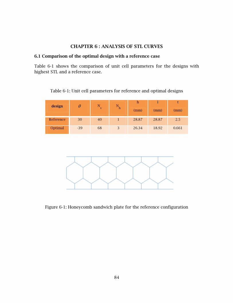
84
CHAPTER 6 : ANALYSIS OF STL CURVES
6.1 Comparison of the optimal design with a reference case
Table 6-1 shows the comparison of unit cell parameters for the designs with
highest STL and a reference case.
Table 6-1: Unit cell parameters for reference and optimal designs
Figure 6-1: Honeycomb sandwich plate for the reference configuration
design Nv N
h
h
(mm)
l
(mm)
t
(mm)
Reference 30 40 1 28.87 28.87 2.5
Optimal -39 68 3 26.34 18.92 0.661

85
Figure 6-2 : Comparison of the STL vs. Frequency plot for the optimal and
reference configuration
Figure 6-3 : Sandwich plate left: reference configuration right: optimal
configuration
Data1: optimal design from case-1
Data2: reference configuration
200 220 240 260 280 300 320 340 360 380 4000
10
20
30
40
50
60
70
80
90
100
Frequency (Hz)
ST
L(d
b)
data1
data2

86
It can be noticed from Figure 6-2 that the optimal design has more area under
the curve. Error! Reference source not found. Table 6-2 shows the auc and the
RMS values for the STL in the frequency range [200, 400] Hz.
Table 6-2: Comparison of the optimal design and reference design
Property Optimal design Reference case % difference
Auc 8700 6794 21.9
RMS value (dB) 43.56 34.80 25.19
Mass (Kg) 73.96050 73.96038 1.6e-4
*
11E (MPa) 7.89 107.82 1266
*
22E (MPa) 4.98 107.82 2065
*
12G (MPa) 0.41 26.95 6473
From the table 6-2 it can be noticed that area under the curve auc and RMS
value of STL of the optimized design are significantly higher than that of the
reference case. Also the mass of both the models is same, as this is a constraint
that has been enforced. It should be noted that the mass in this table is slightly
different than the mass of the sandwich plate mentioned in section 2.2.6. This is
because the mass reported in the table is obtained from ―.DAT‖ file in ABAQUS
whereas the mass reported in the section is calculated from an approximate
formula.
All three stiffness properties of the reference configuration are extremely high
compared to the optimal configuration. These results indicate that the stiffer

87
structure has low STL measure which is consist with findings of Moore et al.
[23] who proposed the use of less stiff in-plane honeycomb sandwich plate over
the stiff out-of-plane configuration. It should also be noted that the reference
configuration has same value of effective Young‘s modulus in the longitudinal
direction *
11E and *
22E Young‘s modulus through the thickness , which is a special
property of honeycomb cores with unit cell angle 30o
[1].
The dips in the STL curve (data-1) correspond to the 15th, 20th and 25th mode of
vibration of the honeycomb plate. These are the flexural modes of vibration.
6.2 Natural Frequencies and mode shapes
Natural frequencies for the optimal design obtained, reported in Table 4-3, are
shown in table 6-3. The natural frequency extraction was done separately using
the ―frequency step‖ in ABAQUS. The natural frequencies are for the sandwich
plate only. The air was not included for the natural frequency extraction.
The dips in the STL of this optimal design correspond to the 15th, 20th and 25th
modes of vibration. These are the odd numbered flexural modes of vibration.
Similar results have been obtained by Griese and Ford et al. in their respective
studies where dips in STL were observed for lower order flexural modes of the
sandwich plate [10][25]. These have been highlighted in Figure 6-3 and their
mode shapes have been shown.

88
Table 6-3: Natural Frequencies of the honeycomb plate of the optimal design
Mode Mode type
Natural
frequency
(Hz)
1 F1 8.43
2 F2 17.15
3 F3 26.50
4 F4 36.67
5 F5 47.86
6 F6 60.23
7 F7 73.91
8 F8 88.97
9 F9 105.4
10 F10 123.47
11 F11 142.96
12 F12 163.94
13 F13 186.39
14 F14 210.29
Mode Mode
type
Natural
frequency
(Hz)
15 F15 235.56
16 D1 248.31
17 F16 262.13
18 D2 262.71
19 D3 278.72
20 F17 289.88
21 D4 297.76
22 F18 318.70
23 D5 318.83
24 D6 340.34
25 F19 348.34
26 D7 361.94
27 F20 378.62
28 D8 383.02
29 D9 403.34

89
To differentiate between the flexural and dilatational modes they have been
identified with different mode types: letter F for flexural modes and letter D for
dilatational modes. The number following the letter identifies the mode number.
6.2.1 The mode shapes of the mode numbers 15, 20 and 25:
Figure 6-4: Mode 15 freq: 235.56 Hz
Figure 6-5: Mode 20 Freq: 289.88 Hz
Figure 6-6: Mode 25 freq: 348.34 Hz
It can be observed from the mode shapes in Figure 6-4, Figure 6-5, Figure 6-6
that they consist of 15, 17 and 19 half sine waves respectively.

90
The natural frequencies between the mode numbers 15 and 20 as well as those
between 20 and 25 do not correspond to any dips in the STL vs. Frequency
graph (Figure 6-2).
6.2.2 The mode shapes corresponding to 16th, 17th, 18th and 19th mode
numbers:
Figure 6-7: Mode 16 freq: 248.31
Figure 6-8: Mode 17 freq: 262.13 Hz
Figure 6-9: Mode 18 freq: 262.71 Hz

91
Figure 6-10: Mode 19 freq: 278.72 Hz
From Figure 6-7, Figure 6-8, Figure 6-9, Figure 6-10 it can be observed that none
of these mode-shapes have odd number of half sine waves. Mode number 17 has
16 half sine waves. Other modes are anti-symmetric or dilatational modes of
vibration.
In the Figure 6-2 no dips are observed to the frequencies corresponding to the
mode numbers 16, 17, 18 and 19.
Figure 6-11: Acoustic region for the fleuxural mode-15.

92
Figure 6-12: Acoustic region for Dilatational mode-16
The sound transmission into the acoustic region for the mode-15 and mode-16
have been shown in Figure 6-11, Figure 6-12 respectively. It can be noticed from
the contours that although the acoustic region for the dilatational mode has
more red colored regions the magnitude of the acoustic pressure is lower for
the dilatational mode compared to the flexural one. This is consistent with the
observation from the Figure 6-2 where no dips correspond to the mode16.
A similar behavior is observed for the modes numbers in between 20 and 25.
None of the modes (21, 22, 23 and 24) have odd number of half sine waves. The
mode numbers 21, 22 and 24 are anti-symmetric or dilatational modes of
vibration. The mode number 23 has 18 half sine waves. These mode shapes
have not been shown.

93
6.2.3 Natural Frequencies of the reference configuration
For the reference case shown in table 6-2 dips in the STL curve correspond to
the mode numbers 3 and 5. The first ten natural frequencies of the honeycomb
sandwich plate (reference configuration) are listed in Table 6-4.
Table 6-4: Natural frequencies of the honeycomb plate of the reference
configuration
Mode number Natural frequency
(Hz)
1 63.43
2 131.16
3 208.22
4 286.29
5 365.18
6 444.45
7 524.40
8 605.01
9 686.37
10 765.90
The modal frequencies corresponding to the mode numbers 3, 4 and 5 are in
the frequency range 200-400 Hz. These modes shapes have been shown in
Figure 6-13, Figure 6-14 and Figure 6-15 respectively. The mode shapes for
modes 3 and 5 have 3 and 5 half sine waves respectively whereas the mode 4
has 4 half sine waves. All these are flexural modes of vibration.

94
Figure 6-13: Mode 3 freq: 208.22 Hz
Figure 6-14: Mode 4 freq: 286.29
Figure 6-15: Mode 5 freq: 365.18

95
6.3 Comparison of the STL curves
Figure 6-16: Comparison of the STL curves of the three designs with the highest
STL and the three with the lowest STL for constant mass of sandwich plate
In Figure 6-16 the data 1, data2 and data3 represent the top three designs in
terms of area under the curve obtained in case-1. The data4, data5 and data6
represent the three lowest designs in terms of area under the curve. The
difference in the STL characteristics of these designs is clearly noticeable in the
graph. Designs with Highest measure of STL have fewer resonant frequencies
the range 200-400Hz, whereas the designs with lowest STL measure have
greater number of resonant frequencies hence the dips in 200-400 Hz.
200 220 240 260 280 300 320 340 360 380 4000
10
20
30
40
50
60
70
80
90
100
Frequency(Hz)
ST
L(d
b)
data1
data2
data3
data4
data5
data6

96
The Table 6-5 shows the values of the area under the curve and the RMS values
of the STL. The design parameters corresponding to these designs have been
shown in Table 6-6.
Table 6-5: STL in terms of area under the curve and RMS values for the 3 designs
with the highest and 3 with the lowest values for 200-400 Hz range
Design Id data auc
RMS value
(dB)
67 data1 8700 43.56
345 data2 8690 43.50
61 data3 8681 43.47
11 data4 5074 26.85
272 data5 5049 26.58
384 data6 5036 26.75
Table 6-6: Honeycomb unit cell parameters correspoding to the designs with the
highest and lowest values of STL measure
Id Nh N
v
h
(mm)
l
(mm)
t
(mm)
67 -39 68 3 26.34 18.92 0.66
345 -29 94 7 12.08 12.16 0.36
61 -41 83 3 24.90 15.96 0.61
11 0 81 8 5.41 12.34 0.44
272 2 76 9 4.35 13.16 0.41
384 -1 50 5 9 20.00 0.70

97
The percentage difference in STL in terms of auc of the data-1 (design with
highest STL measure) and the data-6 (design with the lowest STL measure) is
72%, which is a huge difference. Since the area under the curve auc does not
have any physical significance the RMS values of the STL can also be used as a
performance metric to compare the various designs. There is a considerable
difference in the RMS values of STL between the designs with highest and lowest
values of STL measure. The RMS values are correspondingly high for the designs
with high value of auc. An important observation from the Figure 6-16 is that
the difference between the STL values of any of the designs with lowest value of
STL measure (data -4,5,6) and designs with highest value of STL measure (data-
1,2,3) is at least 6dB, with the exception of the frequencies where the dip in STL
is observed for the best case designs. A difference of 6 dB corresponds to
doubling of the ratio of pi to p
t (equation (3.1)). The following simple
calculations illustrate this point.
10 1020log (4) 20log (2) 6 dB .
For a constant incident pressure an increase of 6 dB implies that the pt has been
reduced to half its value. Thus designs with highest STL show a substantial
improvement over designs with lowest STL. Further the effective stiffness
properties of these six designs have been calculated and compared in Table 6-7.

98
To calculate these properties the formulae shown in section 2.1 have been
used.
Table 6-7: Effective stiffness properties of honeycomb cores corresponding to
designs with the highest and lowest values of STL measure
Id
E11
(MPa)
E22
(MPa)
G12
(MPa)
auc
RMS value
(dB)
67 7.89 4.98 0.41 8700 43.56
345 13.63 1.41 0.36 8690 43.50
61 7.85 8.5 0.48 8681 43.47
11 71.9e3 1.42 3.95 5074 26.85
272 4.9e3 0.81 4.47 5049 26.58
384 24.07e3 1.37 3.56 5036 26.75
For design id 11 the value of Young‘s modulus in the longitudinal direction *
11E
is equal to that of Aluminum. However the value calculated from the equation
(2.6) is infinity, suggesting that the formula is approximate and does not give
accurate values for all values of unit cell geometry, specifically
.
Interesting design trends can be observed from the data presented in Table 6-7.
For designs with high measure of STL the Young‘s modulus in the longitudinal
direction *
11E and shear stiffness *
12G have low values compared to the designs
with low measure of STL. The difference in the values of *
11E is to the order of

99
10e3, whereas for *
12G the difference is to the order of 10. The value of the
Young‘s modulus through the thickness *
22E is high for the designs with high
STL measure and low for designs with low STL. Thus for these designs the STL
measure degrades with increasing stiffness. This finding is consistent with the
results of the study of Moore [23], where the use of a less stiff in-plane
configuration was suggested over an out-of-plane configuration of honeycomb
sandwich plate for higher STL. Furthermore, results from the present study
show that in-plane honeycomb structures having less stiffness give rise to
higher STL, compared to stiffer in-plane configurations.

100
CHAPTER 7 : CONCLUSIONS AND FUTURE WORK
7.1 Accomplishments:
1. An automated design tool has been presented for the optimization of
honeycomb sandwich plate for maximum STL measure using the four
independent geometric variables defining the unit cell of the honeycomb
core with constraints on overall mass and dimensions.
2. The process of creating and solving the ABAQUS based finite element
model has been completely parameterized and automated via Python
scripting.
3. Approximation (RSM) functions have been generated to significantly
expedite the optimization process.
4. The design automation process has been demonstrated for a typical
resonance frequency interval.
5. Optimal designs with high STL have been generated and contrasted with
designs having low STL. Comparisons of effective stiffness properties for
the optimal designs are given.

101
7.2 Conclusions:
1. An automated design tool has been presented for the optimization
problem.
2. An RSM function (using Shepherd K-Nearest algorithm) has been
presented that accurately predicts the output and reduces the run-time of
the optimization drastically.
3. The design parameters that produce the highest STL are 39o N
h = 68
, Nv = 3. This result is specific to the frequency range 200-400Hz.
4. The STL measured in terms of the area under the curve by the output
variable auc is sensitive to all the design variables Nh, N
v and The
significance in the descending order is: Nv, N
h and .
5. Angle between the cells walls of honeycomb and the number of unit
cells in the vertical direction Nv reduce whereas number of the unit cells
in the horizontal direction Nh
increases to increase the STL measured in
terms of area under the curve auc.
6. The odd numbered flexural modes of the sandwich plate correspond to
dips in the STL. However the dilatational modes did not correspond to
any dips in the STL for the frequency range considered in this study.
7. Although a single optimal design has been obtained the designs with Nh
greater than 60, less than -25o and ratio of unit cell lengths h/l

102
greater than 1 perform well to give a high value of auc. Thus a part of
design space has been found to perform well to give high STL.
8. Designs with close to 0o (both positive and negative) and h/l less
than 0.5 have lowest value of auc, and thus the STL performance of these
designs is low.
9. The designs with highest value of STL had low Young‘s modulus in
longitudinal direction *
11E
and shear stiffness *
12G
compared to the
designs with the lowest value of STL measure. However the Young‘s
modulus through the thickness *
22E is high for designs with high STL and
low for those with low STL.
10. For the designs with highest STL measure lower resonances occurred in
the 200-400 Hz frequency range, whereas for designs with low STL
measure higher number of resonances and the corresponding dips in STL
occurred in the considered frequency range.

103
7.3 Future work:
1. Sound Transmission Class (STC) is also used as a single number measure
to quantify the STL characteristics of structures over a frequency range.
This is as per American Society of Testing and Measurement (ASTM)
standard E314 [19]. The STC can be considered as an output measure
instead of the auc or RMS value of STL. The STC is obtained by comparing
the STL curve of the structure with a standard curve. If all the conditions
are satisfied, the value of STL of the standard curve at 500Hz gives the
STC for that structure [19].
2. A stiffness constraint can be added to the existing problem definition to
obtain desired load bearing capacity.
3. Natural frequency extraction can be done to obtain more accurate
resolution for dividing the number of frequency increments within
frequency ranges of the STL vs. Frequency graph for a larger frequency
range.
4. Other frequency ranges can be studied using the developed automatic
design procedures, and compared to see the differences in optimal unit
cell geometries for STL results in different frequency ranges.
5. Experimental validation can be done to study how well the theoretical
results match with the actual STL performance of the sandwich beam.
6. The effect of reflection of sound and different angles of incidence on the
STL characteristics of the sandwich plate can be studied.

104
7. The method presented in this thesis can also be extended to the study of
sandwich structures with different overall dimensions. This can be
achieved easily as the method presented here is completely
parameterized.
8. The developed Python scripts for automatic generation of the Abaqus
based finite element model for the unit cell input geometric variables can
used for other design objectives such as design for high shear flexibility,
lightweight design, and other applications.
105
REFERENCES
[1] Lorna J. Gibson and Michael F. Ashby, 1997, Cellular Solids: Structure and properties.
[2] Schultz J. C., 2011, ―MODELING AND FINITE ELEMENT ANALYSIS METHODS FOR THE DYNAMIC CRUSHING OF HONEYCOMB CELLULAR MESO-STRUCTURES,‖ Clemson University.
[3] Wang D., 2009, ―Impact behavior and energy absorption of paper honeycomb sandwich panels,‖ International Journal of Impact Engineering, 36(1), pp. 110–114.
[4] Evans K. E., 1991, ―The Design of Doubly Curved Sandwich Panels with Honeycomb Cores,‖ Composite Structures, 17, pp. 95–111.
[5] Vinson J. R., 1999, The Behavior of Sandwich Structures of Isotropic and Composite Materials.
[6] Wicks N., and Hutchinson J. W., 2004, ―Performance of sandwich plates with truss cores,‖ Mechanics of Materials, 36(8), pp. 739–751.
[7] Triantafillou T. C., and Gibson L. J., 1987, ―Failure mode maps for foam core sandwich beams,‖ Materials Science and Engineering, 95, pp. 37–53.
[8] Dharmasena K. P., Wadley H. N. G., Xue Z., and Hutchinson J. W., 2008, ―Mechanical response of metallic honeycomb sandwich panel structures to high-intensity dynamic loading,‖ International Journal of Impact Engineering, 35(9), pp. 1063–1074.
[9] Ju J., and Summers J. D., 2011, ―Compliant hexagonal periodic lattice structures having both high shear strength and high shear strain,‖ Materials & Design, 32(2), pp. 512–524.
[10] Griese D. C., 2012, ―FINITE ELEMENT MODELING AND DESIGN OF HONEYCOMB SANDWICH by,‖ (May).
[11] Seera N. K., 2011, ―VISCOELASTIC DAMPING OF HEXAGONAL HONEYCOMB SANDWICH PANELS,‖ Clemson University.
[12] Kumar R. S., and McDowell D. L., 2009, ―Multifunctional design of two-dimensional cellular materials with tailored mesostructure,‖ International Journal of Solids and Structures, 46(14-15), pp. 2871–2885.

106
[13] Ju J., 2009, ―Design of Honeycomb Meta-Materials for High Shear Flexure,‖ ASME 2009 International Design Engineering Technical Conferences and Computers and Information in Engineering, p. 805.
[14] Yamashita M., and Gotoh M., 2005, ―Impact behavior of honeycomb structures with various cell specifications—numerical simulation and experiment,‖ International Journal of Impact Engineering, 32(1-4), pp. 618–630.
[15] Hayes A. M., Wang A., Dempsey B. M., and McDowell D. L., 2004, ―Mechanics of linear cellular alloys,‖ Mechanics of Materials, 36(8), pp. 691–713.
[16] Evans K. E., and Alderson K. L., 2000, ―Auxetic materials : the positive side of being negative,‖ ENGINEERING SCIENCE AND EDUCATION JOURNAL, (August), pp. 148–154.
[17] Ruzzene M., 2004, ―Vibration and sound radiation of sandwich beams with honeycomb truss core,‖ Journal of Sound and Vibration, 277(4-5), pp. 741–763.
[18] Thamburaj P., and Sun J. Q., 2002, ―Optimization of Anisotropic Sandwich Beams for Higher Sound Transmission Loss,‖ Journal of Sound and Vibration, 254(1), pp. 23–36.
[19] Rossing T. D., 2007, Springer Handbook of Acoustics.
[20] Ng C. F., and Hui C. K., 2008, ―Low frequency sound insulation using stiffness control with honeycomb panels,‖ Applied Acoustics, 69(4), pp. 293–301.
[21] Vér I. L., 2006, ―Interaction of Sound Waves with Solid Structures,‖ Noise and vibration control engineering : principles and applications, I.L.V. and L. L.Beranek, ed., Wiley, Hoboken, N.J.
[22] S.Narayanan, and SHANBHAG R. L., 1982, ―SOUND TRANSMISSION THROUGH PANEL DAMPED,‖ Journal of Sound and Vibration, 80(3), pp. 315–327.
[23] Moore J.A. LYON R.H., 1991, ―Sound transmission loss characteristics of sandwich panel constructions,‖ Journal of Acoustical Society of America, 89(2), pp. 777–791.

107
[24] Dym C. L., and Lang M. A., 1974, ―Transmission of sound through sandwich panels,‖ Journal of Acoustical Society of America, 56(5), pp. 1523–1532.
[25] Ford R. D., Lord P., and Walker a. W., 1967, ―Sound transmission through sandwich constructions,‖ Journal of Sound and Vibration, 5(1), pp. 9–21.
[26] B.G.Watters G. K., 1959, ―New Wall Design for High Transmission Loss or High Damping,‖ THE JOURNAL OF THE ACOUSTICAL SOCIETY OF AMERICA, 31(6), pp. 739–748.
[27] Krokosky E. M., and Smolenski C. P., 1973, ―Dilational-mode sound transmission in sandwich panels*,‖ The Journal of the Acoustical Society Acoustical Society of America, 54(6), pp. 1449–1457.
[28] LONDON A., 1950, ―Transmission of Reverberant Sound through Double Walls,‖ THE JOURNAL OF THE ACOUSTICAL SOCIETY OF AMERICA, 22(2).
[29] Lang M. A., and Dym C. L., 1975, ―Optimal acoustic design of sandwich panels,‖ Journal of Acoustical Society of America, 57(6), pp. 1481–1487.
[30] Lin G., and Garrelick J. M., 1977, ―Sound transmission through periodically framed parallel plates,‖ Journal of Acoustical Society of America, 61(4), pp. 1014–1018.
[31] Denli H., and Sun J. Q., 2007, ―Structural-acoustic optimization of sandwich structures with cellular cores for minimum sound radiation,‖ Journal of Sound and Vibration, 301(1-2), pp. 93–105.
[32] Franco F., Cunefare K. a., and Ruzzene M., 2007, ―Structural-Acoustic Optimization of Sandwich Panels,‖ Journal of Vibration and Acoustics, 129(3), p. 330.
[33] El-raheb M., and Wagner P., 1997, ―Transmission of sound across a trusslike periodic panel ; 2-D analysis,‖ Journal of Acoustical Society of America, 102(4), pp. 2176–2183.
[34] Telukunta R., 2011, ―CONSTRAINED LAYER DAMPING OF HONEYCOMB COMPOSITE STRUCTURES,‖ Clemson University.
[35] Ju J., Summers J. D., Ziegert J., and Fadel G., 2012, ―Design of Honeycombs for Modulus and Yield Strain in Shear,‖ Journal of Engineering Materials and Technology, 134(1), p. 011002.

108
[36] ―modeFRONTIER 4.3.0 documentation.‖
[37] ―http://abaqus.civil.uwa.edu.au:2080/v6.9/.‖
[38] Overvelde J. T. B., 2010, ―Learn Abaqus script in one hour,‖ pp. 1–12.
[39] ―Minitab 16 documentation.‖

109
APPENDICES
Appendix A : air_honeycomb_edit_input.py
Python script for generating the honeycomb sandwich plate and
solving it.
001 # -*- coding: mbcs -*-
002 from part import *
003 from material import *
004 from section import *
005 from assembly import *
006 from step import *
007 from interaction import *
008 from load import *
009 from mesh import *
010 from job import *
011 from sketch import *
012 from visualization import *
013 from connectorBehavior import *
014 from math import *
015 from odbAccess import *
016
017
018
019
020 ####### SI units are used
021
022 ##### values for h,l,t, angle, noh, nov are sample values. In the
modeFRONTIER workflow these values are changed in each iteration.
023 h = 28.87e-3
024 l = 28.873e-3
025 t = 2.5e-3
026 angle = 30
027 noh = 40
028 nov = 1
029
030 mdb.models['Model-1'].ConstrainedSketch(name='mysketch',
sheetSize=10.0)
031
032 #### creating a honeycomb unit cell
033 line2 = mdb.models['Model-1'].sketches['mysketch'].Line(point1=(-
3.6, 0.4), point2=(
034 -3.6, 0.4 - h ))
035
036 vertices2 = line2.getVertices() ### retreiving the vertices of
line2

110
037
038 # the line id's and vertices can be found in Figure 0-1. 039
040 x1 = vertices2[1].coords[0] ### x-coordinate of vertex1
041 y1 = vertices2[1].coords[1] ### y-coordinate of vertex1
042
043
044 mdb.models['Model-
1'].sketches['mysketch'].VerticalConstraint(entity=
045 mdb.models['Model-1'].sketches['mysketch'].geometry.findAt((x1,
y1),
046 ))
047
048 # calculating the x & y coordinates of the vertex6 of line3
049 x6 = x1 + l*cos(angle*pi/180) ### x-coordinate of vertex6
050 y6 = y1 - l*sin(angle*pi/180) ### y-coordinate of vertex6
051
052 line3 = mdb.models['Model-
1'].sketches['mysketch'].Line(point1=(x1, y1), point2=
053 (x6, y6))
054
055 # calculating the x & y coordinates of the vertex5 of line4
056 x5 = x1 + 2*l*cos(angle*pi/180) ### x-coordinate of vertex5
057 y5 = y1 ### y-coordinate of vertex5
058
059 line4 = mdb.models['Model-
1'].sketches['mysketch'].Line(point1=(x6,y6 ), point2=
060 (x5, y5))
061
062
063 ##########calculating the x & y coordinates of the vertex4 of line5
064 x4 = x5 ### x-coordinate of vertex4
065 y4 = y5 + h ### y-coordinate of vertex4
066
067 line5 = mdb.models['Model-1'].sketches['mysketch'].Line(point1=(x5,
y5), point2=
068 (x4, y4))
069
070 mdb.models['Model-
1'].sketches['mysketch'].VerticalConstraint(entity=
071 mdb.models['Model-1'].sketches['mysketch'].geometry.findAt((x4,
y4),
072 ))
073
074 ################calculating the x & y coordinates of the vertex3 of
line6
075 x3 = x6 ### x-coordinate of vertex3
076 y3 = y4 + l*sin(angle*pi/180) ### y-coordinate of vertex3
077
078

111
079 line6 = mdb.models['Model-
1'].sketches['mysketch'].Line(point1=(x4,y4), point2=(x3,y3))
080
081 ####################calculating the x & y coordinates of the
vertex2 of line7
082 x2 = x1 ### x-coordinate of vertex2
083 y2 = y1 + h ### y-coordinate of vertex2
084
085 line7 = mdb.models['Model-
1'].sketches['mysketch'].Line(point1=(x3,y3), point2=(x2,y2))
086
087 ##############calculating the x & y coordinates of the vertex7 of
line8
088 x7 = x6 ### x-coordinate of vertex7
089 y7 = y3 + h/2 ### y-coordinate of vertex7
090
091 line8 = mdb.models['Model-
1'].sketches['mysketch'].Line(point1=(x3,y3), point2=(x7,y7))
092
093
094
095 mdb.models['Model-
1'].sketches['mysketch'].VerticalConstraint(entity=
096 mdb.models['Model-1'].sketches['mysketch'].geometry.findAt((x7,
y7),
097 ))
098
099 ##########calculating the x & y coordinates of the vertex8 of line9
100 x8 = x6 ### x-coordinate of vertex8
101 y8 = y6 - h/2 ### y-coordinate of vertex8
102
103 line9 = mdb.models['Model-
1'].sketches['mysketch'].Line(point1=(x6,y6), point2=(x8,y8))
104
105 mdb.models['Model-
1'].sketches['mysketch'].VerticalConstraint(entity=
106 mdb.models['Model-1'].sketches['mysketch'].geometry.findAt((x8,
y8),
107 ))
108
109 mdb.models['Model-1'].sketches['mysketch'].delete(objectList=(
line5, )) #### delete line 5
110
111 mdb.models['Model-1'].sketches['mysketch'].sketchOptions.setValues(
112 displayConstraints=OFF, displayDimensions=OFF)
113
114 ########### linear pattern in the horizontal direction
115 mdb.models['Model-
1'].sketches['mysketch'].linearPattern(angle1=0.0, angle2=
116 90.0, geomList=(
line2,line3,line4,line6,line7,line8,line9),number1= int(noh),

112
number2=1, spacing1= 2*l*cos(angle*pi/180) , spacing2=1.0,
vertexList=())
117
118 ##########calculating the X coordinates of the vertices of the line
to be drawn at the end of the nohth cell
119 ###########Y coordinates are same as that of the line5
120
121 xn = x1 + (noh)*2*l*cos(angle*pi/180)
122 yn = y1
123
124 xm = x2 + (noh)*2*l*cos(angle*pi/180)
125 ym = y2
126
127 mdb.models['Model-1'].sketches['mysketch'].Line(point1=(xn, yn),
point2=(xm, ym)) ##########
draw the missing line in the end
128
129
130 myobject = mdb.models['Model-1'].sketches['mysketch'].geometry
131
132
133 ### vertical linear pattern
134
135 nol = len(myobject)
136
# finding no. of lines in the sketch
137 mylist = []
138
139 for x in range(nol +1):
### line no starts from 2 for some reason
140 if x !=3:
### line 5 has been deleted hence x+2 != 5
141 mylist.insert(x,myobject[x+2])
142
143
144 #### number of replications has to be greater than 1 atleast for
one of the directions. hence we have the if loop.
145 if nov > 1 :
146 mdb.models['Model-
1'].sketches['mysketch'].linearPattern(angle1=0.0, angle2=
147 90.0, geomList= mylist, number1=1, number2= int(nov), spacing1=
2*l*cos(angle*pi/180), spacing2= 2*(h + l*sin(angle*pi/180)) ,
148 vertexList=())
149
150
151
152
153
154
155 mdb.models['Model-1'].Part(dimensionality=TWO_D_PLANAR,
name='core', type=
156 DEFORMABLE_BODY)

113
157 mdb.models['Model-1'].parts['core'].BaseWire(sketch=
158 mdb.models['Model-1'].sketches['mysketch'])
159
160 ############ creating the facesheet
161
162 #############length of the facesheet = noh*2*2*l*cos(angle*pi/180)
163 mdb.models['Model-1'].ConstrainedSketch(name='mysketch1',
sheetSize=10.0)
164
165 mdb.models['Model-1'].sketches['mysketch1'].Line(point1=(-3.2,
0.2), point2=(-3.2 + noh*2*l*cos(angle*pi/180), 0.2))
166
167
168 mdb.models['Model-
1'].sketches['mysketch1'].HorizontalConstraint(entity=
169 mdb.models['Model-1'].sketches['mysketch1'].geometry.findAt((-
3.2, 0.2),
170 ))
171
172
173 mdb.models['Model-1'].Part(dimensionality=TWO_D_PLANAR, name='Part-
2', type=
174 DEFORMABLE_BODY)
175 mdb.models['Model-1'].parts['Part-2'].BaseWire(sketch=
176 mdb.models['Model-1'].sketches['mysketch1'])
177
178 mdb.models['Model-1'].parts.changeKey(fromName='Part-2',
toName='facesheet')
179
180 # ##############creating the semi-circular geometry for air
181
182 mdb.models['Model-1'].ConstrainedSketch(name='mysketch2',
sheetSize=10.0)
183
184 arc = mdb.models['Model-
1'].sketches['mysketch2'].ArcByCenterEnds(center=(0.0, 0.0)
185 , direction=CLOCKWISE, point1=(-noh*2*l*cos(angle*pi/180),
0.0), point2=(noh*2*l*cos(angle*pi/180), 0.0))
186
187 mdb.models['Model-1'].sketches['mysketch2'].Line(point1=(-
noh*2*l*cos(angle*pi/180), 0.0), point2=
188 (noh*2*l*cos(angle*pi/180), 0.0))
189
190
191 mdb.models['Model-
1'].sketches['mysketch2'].HorizontalConstraint(entity=
192 mdb.models['Model-
1'].sketches['mysketch2'].geometry.findAt((0.0, 0.0),
193 ))
194
195

114
196 mdb.models['Model-1'].Part(dimensionality=TWO_D_PLANAR, name='air',
type=
197 DEFORMABLE_BODY)
198 mdb.models['Model-1'].parts['air'].BaseShell(sketch=
199 mdb.models['Model-1'].sketches['mysketch2'])
200
201 ############creating the material
202 ##########Aluminum
203 mdb.models['Model-1'].Material(name='Aluminum')
204 mdb.models['Model-1'].materials['Aluminum'].Density(table=((2700.0,
), ))
205 mdb.models['Model-
1'].materials['Aluminum'].Elastic(table=((719000.0,
206 0.3), ))
207
208 #############air
209 mdb.models['Model-1'].Material(name='air')
210 mdb.models['Model-1'].materials['air'].Density(table=((1.2, ), ))
211 mdb.models['Model-
1'].materials['air'].AcousticMedium(acousticVolumetricDrag=
212 OFF, bulkTable=((141179.0, ), ))
213
214
215 ############ creating sections
216
217 ################beam section
218 mdb.models['Model-1'].RectangularProfile(a= 1, b=t, name=
#### thickness
219 'beam_profile')
220 mdb.models['Model-1'].BeamSection(integration=DURING_ANALYSIS,
material=
221 'Aluminum', name='beamsection', poissonRatio=0.0,
profile='beam_profile',
222 temperatureVar=LINEAR)
223 ######### facesheet beam section
224 mdb.models['Model-1'].RectangularProfile(a= 1, b= 0.0025, name=
#### thickness = 2.5mm
225 'facesheet_beam_profile')
226 mdb.models['Model-1'].BeamSection(integration=DURING_ANALYSIS,
material=
227 'Aluminum', name='facesheet_beamsection', poissonRatio=0.0,
profile='facesheet_beam_profile',
228 temperatureVar=LINEAR)
229
230 ############air section
231 mdb.models['Model-1'].HomogeneousSolidSection(material='air', name=
232 'air_section')
233
234 ########### section assignment
235 ################retreiving all the edges of the "core"
236 alledgescore = mdb.models['Model-1'].parts['core'].edges
237

115
238 #############assigning the beam section to the core
239 mdb.models['Model-1'].parts['core'].SectionAssignment(offset=0.0,
offsetField=
240 '', offsetType=MIDDLE_SURFACE, region=Region(
241 edges=alledgescore), sectionName='beamsection')
242
243 #############assigning beam orientation
244 mdb.models['Model-
1'].parts['core'].assignBeamSectionOrientation(method=
245 N1_COSINES, n1=(0.0, 0.0, -1.0), region=Region(
246 edges= alledgescore ) )
247
248
249
250 ################retreiving the edge of the facesheet
251 alledgesfacesheet = mdb.models['Model-1'].parts['facesheet'].edges
252
253 ##############assigning beam orientation to facesheet
254 mdb.models['Model-
1'].parts['facesheet'].assignBeamSectionOrientation(method=
255 N1_COSINES, n1=(0.0, 0.0, -1.0), region=Region(
256 edges= alledgesfacesheet ) )
257
258 ###########assigning beamsection to facesheet
259 mdb.models['Model-
1'].parts['facesheet'].SectionAssignment(offset=0.0, offsetField=
260 '', offsetType=MIDDLE_SURFACE, region=Region(
261 edges=alledgesfacesheet), sectionName='facesheet_beamsection')
262
263 ####################retreiving the faces of the air
264 allfacesair = mdb.models['Model-1'].parts['air'].faces
265
266 ##################assigning airsection to air
267 mdb.models['Model-1'].parts['air'].SectionAssignment(offset=0.0,
offsetField=
268 '', offsetType=MIDDLE_SURFACE, region=Region(
269 faces=allfacesair), sectionName='air_section')
270
271 ##############3 creating partition on the lower horizontal edge of
air
272
273 #################3retrieving all the edges of the air
274 alledgesair = mdb.models['Model-1'].parts['air'].edges
275
276 ###############setting the edge1 = 0 since this variable has to be
defined before using it
277 edge1 = 0
278
279 #################this loop will retrieve the index of that edge of
the air which has the desired length
280 for x in alledgesair:
281 if x.getSize() == 2*noh*2*l*cos(angle*pi/180):

116
282 edge1 = x.index
283
284
285
286 #####################partitioning the horizontal edge
287 partitionedge1 = mdb.models['Model-
1'].parts['air'].PartitionEdgeByParam(edges= alledgesair[edge1],
288 parameter=0.25)
289
290
291
292
293 partitionedge2 = mdb.models['Model-
1'].parts['air'].PartitionEdgeByParam(edges=
294 mdb.models['Model-
1'].parts['air'].edges.findAt(((noh*l*cos(angle*pi/180), 0.0,0.0), )),
295 parameter=0.67)
296
297
298
299 ###### creating a geometrical set : air (part )
300 ##### mdb.models['Model-1'].parts['air'].Set(name='myset', edges=
mdb.models['Model-
1'].parts['air'].edges.findAt(((noh*l*cos(angle*pi/180), 0.0,0.0), )))
301
302
303 mdb.models['Model-1'].rootAssembly.DatumCsysByDefault(CARTESIAN)
304
305 ############# creating the instances for all the parts
306 mdb.models['Model-1'].rootAssembly.Instance(dependent=ON,
name='air-1', part=
307 mdb.models['Model-1'].parts['air'])
308 mdb.models['Model-1'].rootAssembly.Instance(dependent=ON,
name='core-1', part=
309 mdb.models['Model-1'].parts['core'])
310 mdb.models['Model-1'].rootAssembly.Instance(dependent=ON,
name='facesheet-1',
311 part=mdb.models['Model-1'].parts['facesheet'])
312 mdb.models['Model-1'].rootAssembly.Instance(dependent=ON,
name='facesheet-2',
313 part=mdb.models['Model-1'].parts['facesheet'])
314
315 ###############3 this command seperates the instances
316 mdb.models['Model-1'].rootAssembly.instances['facesheet-
2'].translate(vector=(
317 5.05, 0.0, 0.0))
318
319
320
321 ############### translating the facesheet on the top and bottom of
the honeycomb core
322

117
323 ##################translating facesheet-1 to the top of the core
324 ################create the vector to translate the facesheet
325 ##############3for this we select the left corner of the facesheet
and top left corner of the core
326
327 ################3coordinates of the bottom & top left corners of
the core
328
329 ############3bottom left
330 xb = x1
331 yb = y1 - (l*sin(angle*pi/180) + h/2)
332
333 #############top left
334 xt = x1
335 yt = yb + nov*2*(h + l*sin(angle*pi/180) )
336
337
338 ###### retrieving the coordinates of left corner of the facesheet-1
339 ########## to do this we get the coordinates of the both the
vertices of the facesheet-1 and the compare the x-coordinate
340 ############ the one with lesser value is the left corner vertex
341
342 verticesfs1 = mdb.models['Model-
1'].rootAssembly.instances['facesheet-1'].vertices
343
344 #################retreiving the coordinates of the vertices
345 vx1 = verticesfs1[0].pointOn
346 vx2 = verticesfs1[1].pointOn
347
348 ################defining a variable before using it
349 index = 1
350
351 ############ grabbing the left vertex of the facesheet
352 if vx1[0][0] < vx2[0][0]:
353 index = 0
354 if vx1[0][0] >= vx2[0][0]:
355 index = 1
356
357 ################vertex of interest
358 vi = verticesfs1[index]
359
360
361
362 #################vector for translating facesheet-1
363
364 vector1 = xt - vi.pointOn[0][0], yt - vi.pointOn[0][1], 0
365
366
367 ###################translating facesheet-1
368 mdb.models['Model-
1'].rootAssembly.translate(instanceList=('facesheet-1', ),
369 vector= vector1)

118
370
371
372 ##############similarly translating facesheet-2
373
374 verticesfs2 = mdb.models['Model-
1'].rootAssembly.instances['facesheet-2'].vertices
375
376 ##############retreiving the coordinates of the vertices
377 vx3 = verticesfs2[0].pointOn
378 vx4 = verticesfs2[1].pointOn
379
380 ###################defining a variable before using it
381 index = 1
382
383
384 if vx3[0][0] < vx4[0][0]:
385 index = 0
386 if vx3[0][0] >= vx4[0][0]:
387 index = 1
388
389 ###############vertex of interest
390 vj = verticesfs2[index]
391
392
393
394 ################vector for translating facesheet-2
395
396 vector2 = xb - vj.pointOn[0][0], yb - vj.pointOn[0][1], 0
397
398
399 ################translating facesheet-2
400 mdb.models['Model-
1'].rootAssembly.translate(instanceList=('facesheet-2', ),
401 vector= vector2)
402
403
404 ############## translating air to it position on top of the core
405 verticesair = mdb.models['Model-1'].rootAssembly.instances['air-
1'].vertices
406
407
408 index1 = 2
409
410 #####################retrieving the left most vertex of the
horizontal edge of air to create the vector for translating air
411
412
413 if verticesair[0].pointOn[0][0] < verticesair[1].pointOn[0][0]
and verticesair[0].pointOn[0][0] < verticesair[2].pointOn[0][0] and
verticesair[0].pointOn[0][0] < verticesair[3].pointOn[0][0] :
414 index1 = verticesair[0].index

119
415 if verticesair[1].pointOn[0][0] < verticesair[0].pointOn[0][0]
and verticesair[1].pointOn[0][0] < verticesair[2].pointOn[0][0] and
verticesair[1].pointOn[0][0] < verticesair[3].pointOn[0][0] :
416 index1 = verticesair[1].index
417 if verticesair[2].pointOn[0][0] < verticesair[1].pointOn[0][0]
and verticesair[2].pointOn[0][0] < verticesair[0].pointOn[0][0] and
verticesair[2].pointOn[0][0] < verticesair[3].pointOn[0][0] :
418 index1 = verticesair[2].index
419 if verticesair[3].pointOn[0][0] < verticesair[0].pointOn[0][0]
and verticesair[3].pointOn[0][0] < verticesair[1].pointOn[0][0] and
verticesair[3].pointOn[0][0] < verticesair[2].pointOn[0][0] :
420 index1 = verticesair[3].index
421
422 ############index1 is the index of the required vertex
423 ##############vertex is the starting point for the vector
424
425 ##################end point of the vector - assuming that the
raduis of the air is equal to length of beam
426
427 xe = xt - noh*l*cos(angle*pi/180)
428 ye = yt
429
430 vk = verticesair[index1]
431 #############vector for translating
432 vector3 = xe - vk.pointOn[0][0], ye - vk.pointOn[0][1],0
433
434
435 ############traslating air to the its final position
436 mdb.models['Model-1'].rootAssembly.translate(instanceList=('air-1',
),
437 vector= vector3)
438 ###########
439
440
441 alledgesair2 = mdb.models['Model-1'].rootAssembly.instances['air-
1'].edges
442 edgemiddle1 = 9
443 for x in alledgesair2:
444 if round(x.getSize(),1) == round(noh*2*l*cos(angle*pi/180),1):
445 edgemiddle1 = x.index
446
447
448
449 ###### creating a geometrical set : air-1
450 mdb.models['Model-1'].rootAssembly.Set(name='myset', edges=
mdb.models['Model-1'].rootAssembly.instances['air-1'].edges.findAt(
451 ((xt + noh*l*cos(angle*pi/180),yt , 0.0), ), ))
452
453
454 ################creating steps & field output requests
455

120
456 mdb.models['Model-1'].SteadyStateDirectStep(frequencyRange=((200,
400, 100,
457 1.0), ), name='Step-1', previous='Initial', scale=LINEAR)
458 mdb.models['Model-1'].fieldOutputRequests['F-Output-
1'].setValues(variables=(
459 'S', 'U', 'V', 'A', 'POR', 'ACV', 'GRADP', 'INTEN'))
460
461
462 ####### history output request
463 regionDef=mdb.models['Model-1'].rootAssembly.sets['myset']
464
465
466 mdb.models['Model-1'].HistoryOutputRequest(name='H-Output-2',
467 createStepName='Step-1', variables=('POR', ), region=regionDef,
468 sectionPoints=DEFAULT, rebar=EXCLUDE)
469
470 index2 = 7
471 for x in alledgesair:
472 if x.getSize() == pi*2*noh*l*cos(angle*pi/180):
473 index2 = x.index
474 print alledgesair[0]
475
476 #################creating an interaction i.e. a non-reflecting BC
on the curved edge of the air
477
478 mdb.models['Model-1'].AcousticImpedance(createStepName='Step-1',
definition=
479 NONREFLECTING, name='Int-1', nonreflectingType=CIRCULAR,
radius= 2*noh*l*cos(angle*pi/180),
480 surface=Region(
481 side1Edges=mdb.models['Model-1'].rootAssembly.instances['air-
1'].edges.findAt(
482 ((xt + noh*l*cos(angle*pi/180),yt + 2*noh*l*cos(angle*pi/180) ,
0.0), ), )))
483
484
485 ######## creating BC
486
487 ####### pinned BC for the left side of the plate
488 ########edges
489
490 for x in range(nov):
491 mdb.models['Model-1'].DisplacementBC(amplitude=UNSET,
createStepName='Step-1',
492 distributionType=UNIFORM, fieldName='', fixed=OFF,
localCsys=None, name=
493 'BC' + str(x + 1 ), region=Region(
494 edges=mdb.models['Model-1'].rootAssembly.instances['core-
1'].edges.findAt(
495 ((xb,yb + (l*sin(angle*pi/180) + h) +
x*2*(l*sin(angle*pi/180) + h) ,0),) )), u1=0j
496 , u2=0j, ur3=UNSET)
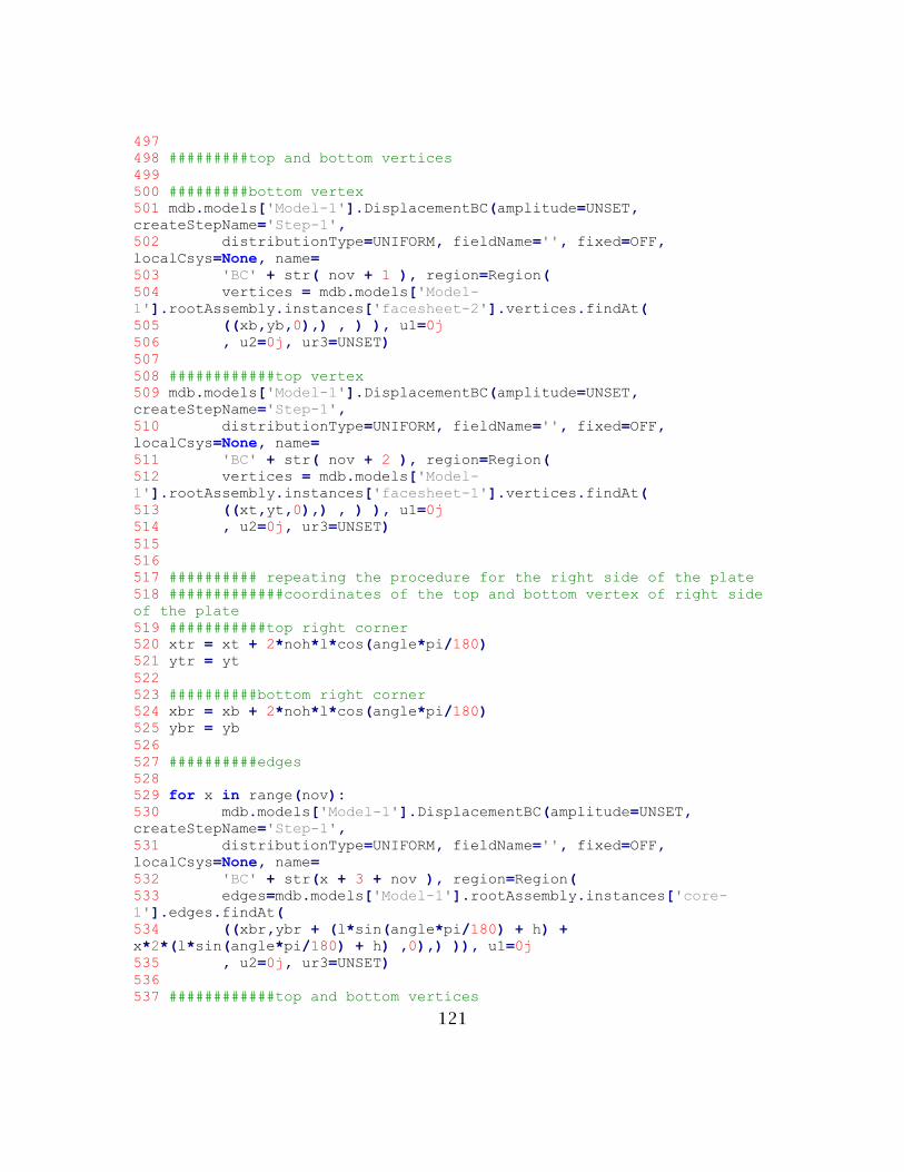
121
497
498 #########top and bottom vertices
499
500 #########bottom vertex
501 mdb.models['Model-1'].DisplacementBC(amplitude=UNSET,
createStepName='Step-1',
502 distributionType=UNIFORM, fieldName='', fixed=OFF,
localCsys=None, name=
503 'BC' + str( nov + 1 ), region=Region(
504 vertices = mdb.models['Model-
1'].rootAssembly.instances['facesheet-2'].vertices.findAt(
505 ((xb,yb,0),) , ) ), u1=0j
506 , u2=0j, ur3=UNSET)
507
508 ############top vertex
509 mdb.models['Model-1'].DisplacementBC(amplitude=UNSET,
createStepName='Step-1',
510 distributionType=UNIFORM, fieldName='', fixed=OFF,
localCsys=None, name=
511 'BC' + str( nov + 2 ), region=Region(
512 vertices = mdb.models['Model-
1'].rootAssembly.instances['facesheet-1'].vertices.findAt(
513 ((xt,yt,0),) , ) ), u1=0j
514 , u2=0j, ur3=UNSET)
515
516
517 ########## repeating the procedure for the right side of the plate
518 #############coordinates of the top and bottom vertex of right side
of the plate
519 ###########top right corner
520 xtr = xt + 2*noh*l*cos(angle*pi/180)
521 ytr = yt
522
523 ##########bottom right corner
524 xbr = xb + 2*noh*l*cos(angle*pi/180)
525 ybr = yb
526
527 ##########edges
528
529 for x in range(nov):
530 mdb.models['Model-1'].DisplacementBC(amplitude=UNSET,
createStepName='Step-1',
531 distributionType=UNIFORM, fieldName='', fixed=OFF,
localCsys=None, name=
532 'BC' + str(x + 3 + nov ), region=Region(
533 edges=mdb.models['Model-1'].rootAssembly.instances['core-
1'].edges.findAt(
534 ((xbr,ybr + (l*sin(angle*pi/180) + h) +
x*2*(l*sin(angle*pi/180) + h) ,0),) )), u1=0j
535 , u2=0j, ur3=UNSET)
536
537 ############top and bottom vertices

122
538
539 ###########bottom vertex
540 mdb.models['Model-1'].DisplacementBC(amplitude=UNSET,
createStepName='Step-1',
541 distributionType=UNIFORM, fieldName='', fixed=OFF,
localCsys=None, name=
542 'BC' + str( 2*nov + 3 ), region=Region(
543 vertices = mdb.models['Model-
1'].rootAssembly.instances['facesheet-2'].vertices.findAt(
544 ((xbr,ybr,0),) , ) ), u1=0j
545 , u2=0j, ur3=UNSET)
546
547 #############top vertex
548 mdb.models['Model-1'].DisplacementBC(amplitude=UNSET,
createStepName='Step-1',
549 distributionType=UNIFORM, fieldName='', fixed=OFF,
localCsys=None, name=
550 'BC' + str( 2*nov + 4 ), region=Region(
551 vertices = mdb.models['Model-
1'].rootAssembly.instances['facesheet-1'].vertices.findAt(
552 ((xtr,ytr,0),) , ) ), u1=0j
553 , u2=0j, ur3=UNSET)
554
555
556 #################applying load on the lower facesheet
557 mdb.models['Model-1'].Pressure(amplitude=UNSET,
createStepName='Step-1',
558 distributionType=UNIFORM, field='', magnitude=(1+0j),
name='Load-1',
559 region=Region(
560 side2Edges=mdb.models['Model-
1'].rootAssembly.instances['facesheet-2'].edges.findAt(
561 ((xb,yb, 0.0), ), )))
562
563 ###### meshing
564
565 #######meshing air
566 ########setting mesh controls for air
567 mdb.models['Model-1'].parts['air'].setMeshControls(elemShape=TRI,
regions=
568 mdb.models['Model-1'].parts['air'].faces)
569
570 #########assigning acoustic elements
571 mdb.models['Model-
1'].parts['air'].setElementType(elemTypes=(ElemType(
572 elemCode=AC2D4, elemLibrary=STANDARD), ElemType(elemCode=AC2D3,
573 elemLibrary=STANDARD)), regions=(
574 mdb.models['Model-1'].parts['air'].faces, ))
575
576
577
578

123
579 #########setting bias for the edges
580 #################bias for middle part of the partitioned lower edge
of air
581 ############retrieving index for the middle part of the edge
582
583 alledgesair1 = mdb.models['Model-1'].parts['air'].edges
584 edgemiddle = 9 ## setting this variable to a random value to use
it further
585 edgeendl = 9 ## setting this variable to a random value to use it
further
586 edgeendlr = 9 ## setting this variable to a random value to use it
further
587 edgecurve = 9 ## setting this variable to a random value to use it
further
588
589 for x in alledgesair1:
590 if round(x.getSize(),1) == round(noh*2*l*cos(angle*pi/180),1):
591 edgemiddle = x.index
592
593
594 mdb.models['Model-1'].parts['air'].seedEdgeByBias(end1Edges=
595 ((mdb.models['Model-1'].parts['air'].edges[edgemiddle]),),
596 number=100, ratio=1.0)
597
598 ##########retrieving the index of the left part of the partitioned
edge
599 for x in alledgesair1:
600 if round(x.getSize(),1) == round(noh*l*cos(angle*pi/180),1):
601 edgeendl = x.index
602 ########seed bias for left part of the partitioned edge
603 mdb.models['Model-1'].parts['air'].seedEdgeByBias(end1Edges=
604 ((mdb.models['Model-1'].parts['air'].edges[edgeendl]),),
605 number=50, ratio=3.0)
606
607 ############retrieving the index of the right part of the
partitioned edge
608 for x in alledgesair1:
609 if round(x.getSize(),1) == round(noh*l*cos(angle*pi/180),1) and
x.index != edgeendl:
610 edgeendr = x.index
611
612
613 ############seed bias for the right part of the partitioned edge of
air
614 mdb.models['Model-1'].parts['air'].seedEdgeByBias(end2Edges=
615 ((mdb.models['Model-1'].parts['air'].edges[edgeendr]),),
616 number=50, ratio=3.0)
617
618 #############retrieving index of the curved edge
619 for x in alledgesair:
620 if round(x.getSize(),1) ==
round(pi*2*noh*l*cos(angle*pi/180),1):

124
621 edgecurve = x.index
622
623 ############seed bias for the curved edge
624 mdb.models['Model-1'].parts['air'].seedEdgeBySize(edges=
625 ((mdb.models['Model-1'].parts['air'].edges[edgecurve]),),
size=0.08)
626
627 ###########generating mesh on air
628 mdb.models['Model-1'].parts['air'].generateMesh()
629
630 ################assigning element type to the core
631 mdb.models['Model-
1'].parts['core'].setElementType(elemTypes=(ElemType(
632 elemCode=B22, elemLibrary=STANDARD), ), regions=(
633 ((mdb.models['Model-1'].parts['core'].edges),) ))
634 ##########seeding and meshing the core
635 mdb.models['Model-1'].parts['core'].seedPart(deviationFactor=0.1,
size=0.005)
636 mdb.models['Model-1'].parts['core'].generateMesh()
637
638 ############assigning element type to the facesheet
639 mdb.models['Model-
1'].parts['facesheet'].setElementType(elemTypes=(ElemType(
640 elemCode=B22, elemLibrary=STANDARD), ), regions=(
641 ((mdb.models['Model-1'].parts['facesheet'].edges),) ,))
642
643 ###########seeding and meshing the facesheet
644 mdb.models['Model-
1'].parts['facesheet'].seedPart(deviationFactor=0.1, size=
645 0.006)
646 mdb.models['Model-1'].parts['facesheet'].generateMesh()
647
648 ###### creating the tie constraints
649
650 ###########tie constraints at the bottom for the core and
facesheet-2
651 edges11 = mdb.models['Model-1'].rootAssembly.instances['facesheet-
1'].edges
652 edges22 = mdb.models['Model-1'].rootAssembly.instances['facesheet-
2'].edges
653 ecl1 = []
654
655 for i in range(noh):
656 ecl1.insert(i,(xb + l*cos(angle*pi/180)
+i*2*l*cos(angle*pi/180),yb,0))
657
658
659 ######### creating tie constraints. Each execution of the for loop
creates a constraint. We create noh no. of constraints
660
661 ############ constraints at the bottom

125
662 s1 = mdb.models['Model-1'].rootAssembly.instances['core-
1'].vertices
663
664 for x in range(len(ecl1)):
665
666 vertices11 = s1.findAt( (ecl1[x],))
667 mdb.models['Model-1'].Tie(adjust=ON, master=Region(
668 edges = edges22),name='Constraint' + str(x),
669 positionToleranceMethod=COMPUTED,slave=Region(
670 vertices = vertices11 ), thickness=ON,
671 tieRotations=ON)
672
673 #############repeating the same procedure for the top facesheet and
core
674 ecl2 = []
675
676 for i in range(noh):
677 ecl2.insert(i,(xt + l*cos(angle*pi/180)
+i*2*l*cos(angle*pi/180),yt,0))
678
679
680 ###### creating tie constraints. Each execution of the for loop
creates a constraint. We create noh no. of constraints
681
682 ####### constraints at the top
683 s2 = mdb.models['Model-1'].rootAssembly.instances['core-
1'].vertices
684
685 for x in range(len(ecl2)):
686
687 vertices22 = s2.findAt( (ecl2[x],))
688 mdb.models['Model-1'].Tie(adjust=ON, master=Region(
689 edges = edges11),name='Constraint' + str(x + len(ecl1) ),
690 positionToleranceMethod=COMPUTED,slave=Region(
691 vertices = vertices22 ), thickness=ON,
692 tieRotations=ON)
693
694 ###tie constraints for air & the facesheet-1
695 #########3master = facesheet-2 and slave = middle part of the
partitioned edge of air
696 pointmm = mdb.models['Model-1'].rootAssembly.instances['air-
1'].edges[edgemiddle].pointOn
697
698 mdb.models['Model-1'].Tie(adjust=ON, master=Region(
699 side1Edges = edges11),name='Constraint' + str( len(ecl2) +
len(ecl1) + 1 ),
700 positionToleranceMethod=COMPUTED,slave=Region(
701 side1Edges = mdb.models['Model-
1'].rootAssembly.instances['air-1'].edges.findAt(pointmm,) ),
thickness=ON,
702 tieRotations=ON)
703

126
704
705 ########creating job
706 mdb.Job(atTime=None, contactPrint=OFF, description='',
echoPrint=OFF,
707 explicitPrecision=SINGLE, getMemoryFromAnalysis=True,
historyPrint=OFF,
708 memory=90, memoryUnits=PERCENTAGE, model='Model-1',
modelPrint=OFF,
709 multiprocessingMode=DEFAULT, name='Job-1',
nodalOutputPrecision=SINGLE,
710 numCpus=1, numDomains=1, parallelizationMethodExplicit=DOMAIN,
queue=None,
711 scratch='', type=ANALYSIS, userSubroutine='', waitHours=0,
waitMinutes=0)
712
713 mdb.jobs['Job-1'].submit(consistencyChecking=OFF)
714
715 mdb.jobs['Job-1']._Message(ODB_FILE, {'phase': BATCHPRE_PHASE,
716 'file': '.\\Job-1.odb', 'jobName': 'Job-1'})
Figure 0-1: Unit cell line and vertex numbering

127
Appendix B: output_air_honeycomb_edit.py
001 from abaqus import *
002 from abaqusConstants import *
003 from math import *
004 from odbAccess import *
005 from caeModules import *
006 from viewerModules import *
007 from driverUtils import executeOnCaeStartup
008 session.Viewport(name='Viewport: 1', origin=(0.0, 0.0),
width=238.177169799805,
009 height=151.02604675293)
010 session.viewports['Viewport: 1'].makeCurrent()
011 session.viewports['Viewport: 1'].maximize()
012
013 executeOnCaeStartup()
014
015 a = mdb.models['Model-1'].rootAssembly
016
017 session.viewports['Viewport: 1'].setValues(displayedObject=a)
018 o3 = session.openOdb(
019 name='Job-1.odb')
020 session.viewports['Viewport: 1'].setValues(displayedObject=o3)
021
022
023
024 #### session.odbs is the repository which contains the opened odb
file
025 myodb = session.odbs['Job-1.odb']
026 # session.viewports['Viewport:
1'].odbDisplay.basicOptions.setValues(
027 # numericForm=COMPLEX_MAGNITUDE)
028 ######### retrieving the number of frames in the odb
029 frame_no = myodb.steps['Step-1'].frames
030
031 #### fetching the number of nodes in the partitioned part of the
air
032
033
034 ######## we want the values of POR for the entire nodeset MYSET for
individual frequency/frame in a seperate index in the list mydata
035
036
037 mydata = [] ###### values of POR of all the nodes in the
nodeset MYSET for individual frames
038 mysrss = [] ###### rms value of POR for the nodes in MYSET for
each frequency
039 mystl = [] ###### sound transmission loss at each frequency
040 mycurve = [] ###### freq & stl values
041 for x in frame_no:
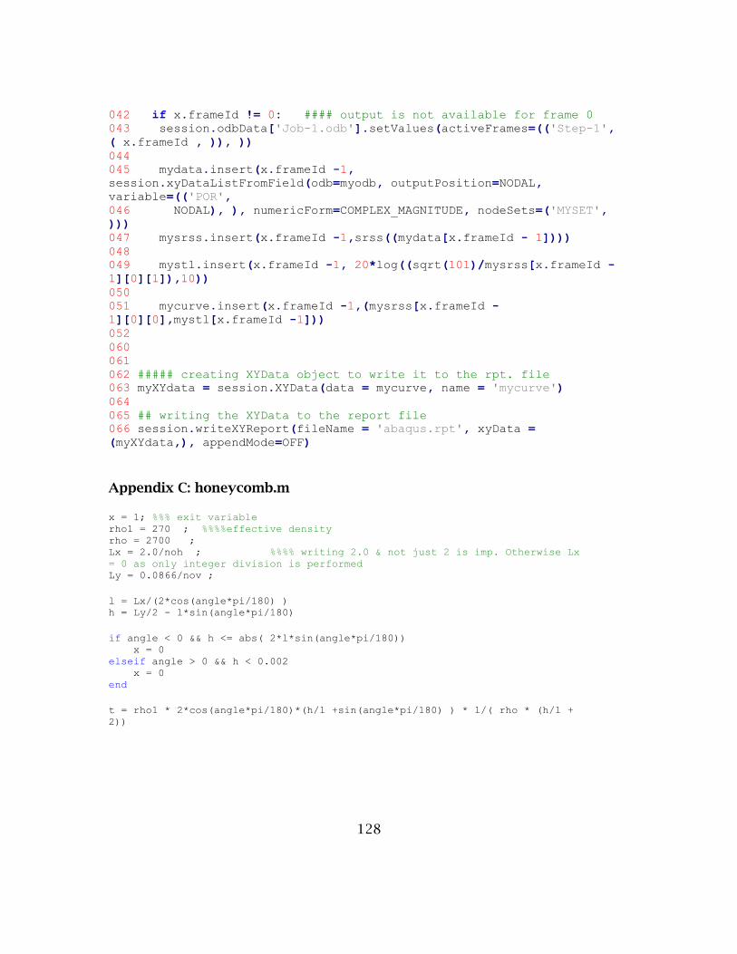
128
042 if x.frameId != 0: #### output is not available for frame 0
043 session.odbData['Job-1.odb'].setValues(activeFrames=(('Step-1',
( x.frameId , )), ))
044
045 mydata.insert(x.frameId -1,
session.xyDataListFromField(odb=myodb, outputPosition=NODAL,
variable=(('POR',
046 NODAL), ), numericForm=COMPLEX_MAGNITUDE, nodeSets=('MYSET',
)))
047 mysrss.insert(x.frameId -1,srss((mydata[x.frameId - 1])))
048
049 mystl.insert(x.frameId -1, 20*log((sqrt(101)/mysrss[x.frameId -
1][0][1]),10))
050
051 mycurve.insert(x.frameId -1,(mysrss[x.frameId -
1][0][0],mystl[x.frameId -1]))
052
060
061
062 ##### creating XYData object to write it to the rpt. file
063 myXYdata = session.XYData(data = mycurve, name = 'mycurve')
064
065 ## writing the XYData to the report file
066 session.writeXYReport(fileName = 'abaqus.rpt', xyData =
(myXYdata,), appendMode=OFF)
Appendix C: honeycomb.m x = 1; %%% exit variable rho1 = 270 ; %%%%effective density rho = 2700 ; Lx = 2.0/noh ; %%%% writing 2.0 & not just 2 is imp. Otherwise Lx
= 0 as only integer division is performed Ly = 0.0866/nov ;
l = Lx/(2*cos(angle*pi/180) ) h = Ly/2 - l*sin(angle*pi/180)
if angle < 0 && h <= abs( 2*l*sin(angle*pi/180)) x = 0 elseif angle > 0 && h < 0.002 x = 0 end
t = rho1 * 2*cos(angle*pi/180)*(h/l +sin(angle*pi/180) ) * l/( rho * (h/l +
2))

129
Appendix D: matlab_output.m
h = figure; plot(X,Y) xlabel('Frequency (Hz)'); ylabel('STL (db)') AXIS([200 400 0 100]); saveas(h,'figure1.m')
auc = trapz(X,Y)
Appendix E: input.bat
rem cd C:\Temp
abaqus cae noGUI=air_honeycomb_edit_input.py
Appendix F: output. Bat
abaqus cae noGUI=output_air_honeycomb_edit.py
Appendix G: DOE case-1 design table:
<ID> <CATEGORY>
Nh Nv h l t auc
0 ULH 41 35 7 -0.01865 0.037858 6.19E-04 NaN
1 ULH 44 96 1 0.033241 0.014481 0.00145 7863.361
2 ULH -35 65 5 0.019432 0.018781 4.68E-04 NaN
3 ULH 13 34 8 -0.00138 0.030185 5.40E-04 NaN
4 ULH -39 26 9 0.035957 0.049491 2.74E-04 NaN
5 ULH 30 87 4 0.004189 0.013272 8.10E-04 6914.042
6 ULH -24 43 7 0.01654 0.025457 4.27E-04 NaN
7 ULH -32 53 2 0.03344 0.022249 0.001048 8617.263
8 ULH 43 80 10 -0.00733 0.017092 4.03E-04 NaN
9 ULH 5 91 2 0.020689 0.011031 0.001113 7971.405

130
10 ULH -18 35 10 0.013613 0.030042 3.36E-04 NaN
11 ULH 0 81 8 0.005413 0.012346 4.44E-04 5074.777
12 ULH -21 100 9 0.00865 0.010711 3.20E-04 8598.651
13 ULH -31 73 5 0.016891 0.015981 4.86E-04 8638.165
14 ULH -9 49 7 0.009418 0.020663 4.98E-04 8253.534
15 ULH -35 64 8 0.016353 0.019075 3.10E-04 NaN
16 ULH -27 67 4 0.01843 0.016751 6.22E-04 8578.397
17 ULH 17 47 3 0.007928 0.022249 0.001172 7021.134
18 ULH 9 55 4 0.007945 0.018408 8.79E-04 7917.452
19 ULH 3 74 3 0.013725 0.013532 9.56E-04 7938.947
20 ULH 32 45 7 -0.0077 0.026204 6.15E-04 NaN
21 ULH -23 22 3 0.033728 0.04938 9.90E-04 NaN
22 ULH 18 68 8 6.34E-04 0.015463 5.04E-04 NaN
23 ULH 9 72 6 0.005017 0.014062 6.05E-04 7848.316
24 ULH -19 22 4 0.026476 0.048074 8.03E-04 NaN
25 ULH -23 69 10 0.010482 0.015744 2.99E-04 NaN
26 ULH 5 73 2 0.020452 0.013751 0.001237 7976.152
27 ULH -11 94 1 0.045368 0.010837 0.001374 8278.675
28 ULH 15 39 10 -0.00254 0.026546 4.39E-04 NaN
29 ULH 13 59 7 0.002273 0.017395 5.66E-04 6630.6
30 ULH -9 25 5 0.014995 0.040499 7.22E-04 7722.938
31 ULH 0 37 7 0.006186 0.027027 5.55E-04 6026
32 ULH -19 59 1 0.049136 0.017926 0.001727 8226.713
33 ULH -1 70 8 0.005662 0.014288 4.52E-04 5309.157
34 ULH 45 75 1 0.029967 0.018856 0.001706 7832.647
35 ULH 37 37 6 -0.01315 0.033842 7.15E-04 NaN
36 ULH 24 99 1 0.038803 0.011057 0.001436 7995.971
37 ULH -5 20 4 0.015199 0.050191 9.37E-04 5397.164
38 ULH 1 99 5 0.008484 0.010103 6.10E-04 7998.389
39 ULH 15 21 9 -0.00795 0.049299 5.05E-04 NaN
40 ULH 30 81 4 0.003697 0.014256 8.30E-04 6920.63
41 ULH 40 37 8 -0.01727 0.035281 5.49E-04 NaN
42 ULH -24 70 10 0.01069 0.015638 2.95E-04 NaN
43 ULH 1 71 2 0.021404 0.014087 0.00123 7847.009
44 ULH 4 84 2 0.020818 0.011934 0.001154 7954.496
45 ULH 38 41 2 0.002594 0.030952 0.001637 8565.755
46 ULH 15 50 10 -0.00103 0.020706 4.29E-04 NaN

131
47 ULH -28 35 7 0.021377 0.032359 4.11E-04 NaN
48 ULH -15 22 7 0.018365 0.047058 5.00E-04 NaN
49 ULH 10 39 8 8.91E-04 0.026037 5.24E-04 NaN
50 ULH 25 58 7 -0.00185 0.019024 5.89E-04 NaN
51 ULH -27 99 6 0.012363 0.011337 4.16E-04 8645.197
52 ULH 43 61 7 -0.0091 0.022415 5.68E-04 NaN
53 ULH -39 32 7 0.031491 0.040211 3.45E-04 NaN
54 ULH 10 80 8 0.003208 0.012693 4.73E-04 7742.415
55 ULH -17 44 1 0.050248 0.023766 0.002013 8176.115
56 ULH -20 38 8 0.014991 0.028005 4.01E-04 NaN
57 ULH 11 53 10 6.62E-04 0.019221 4.18E-04 NaN
58 ULH 31 58 7 -0.00417 0.020114 5.92E-04 NaN
59 ULH 12 55 8 0.001548 0.018588 5.08E-04 NaN
60 ULH -21 25 4 0.02618 0.042846 7.74E-04 NaN
61 ULH -41 83 3 0.024907 0.015964 6.12E-04 8681.482
62 ULH -32 76 2 0.029872 0.015516 9.35E-04 8488.3
63 ULH -5 59 1 0.044783 0.017014 0.001862 7866.684
64 ULH -24 99 1 0.047797 0.011057 0.001251 8396.733
65 ULH -13 75 10 0.007408 0.013684 3.32E-04 8489.3
66 ULH 2 21 9 0.003148 0.047648 4.65E-04 6140.812
67 ULH -39 68 3 0.026342 0.018923 6.61E-04 8700.046
68 ULH -5 62 2 0.023061 0.016191 0.00126 8243.912
69 ULH -33 51 6 0.01995 0.02338 4.24E-04 NaN
70 ULH 39 40 7 -0.01406 0.032169 6.15E-04 NaN
71 ULH 20 41 9 -0.00407 0.025956 4.91E-04 NaN
72 ULH 19 47 6 -1.09E-04 0.022503 6.84E-04 NaN
73 ULH -21 95 1 0.047341 0.011275 0.001304 8282.847
74 ULH -7 33 9 0.008532 0.030531 4.19E-04 5293.529
75 ULH 45 80 1 0.0308 0.017678 0.001636 7836.32
76 ULH -14 27 6 0.016451 0.038171 5.76E-04 NaN
77 ULH -28 50 9 0.015445 0.022651 3.17E-04 NaN
78 ULH 34 77 4 0.002065 0.015665 8.42E-04 8354.244
79 ULH 25 23 1 0.023026 0.047973 0.003165 7001.969
80 ULH -6 34 6 0.010308 0.029574 6.11E-04 7183.665
81 ULH 6 57 6 0.005373 0.01764 6.23E-04 7690.837
82 ULH 17 46 7 -4.61E-04 0.022732 5.98E-04 NaN
83 ULH 21 24 10 -0.01166 0.044631 4.65E-04 NaN

132
84 ULH -45 43 9 0.028067 0.032889 2.38E-04 NaN
85 ULH -16 41 6 0.01421 0.025373 5.42E-04 8319.927
86 ULH 18 78 5 0.004494 0.01348 7.06E-04 6766.676
87 ULH 7 91 1 0.041951 0.011072 0.001485 7865.467
88 ULH -2 57 3 0.015046 0.017555 0.00101 7985.752
89 ULH -42 61 2 0.036411 0.02206 8.81E-04 8598.213
90 ULH -7 55 2 0.023882 0.018318 0.001301 8174.911
91 ULH -35 78 7 0.015163 0.015651 3.41E-04 NaN
92 ULH 15 96 1 0.040509 0.010784 0.001453 8009.943
93 ULH 11 41 4 0.006084 0.024847 9.47E-04 7627.729
94 ULH 24 70 10 -0.00203 0.015638 4.23E-04 NaN
95 ULH -20 47 9 0.012555 0.022642 3.54E-04 NaN
96 ULH 6 52 5 0.006639 0.019337 7.35E-04 7891.035
97 ULH -41 42 3 0.035131 0.031548 7.00E-04 NaN
98 ULH 11 42 8 7.84E-04 0.024255 5.23E-04 NaN
99 ULH 19 65 1 0.038003 0.016271 0.001889 7706.941
100 ULH -30 60 6 0.016839 0.019245 4.35E-04 NaN
101 ULH 44 56 8 -0.01183 0.024824 5.11E-04 NaN
102 ULH 21 84 1 0.03873 0.012752 0.001605 7872.67
103 ULH -9 90 10 0.00609 0.01125 3.37E-04 8404.599
104 ULH 22 79 3 0.009319 0.013652 9.98E-04 7353.652
105 ULH -23 93 2 0.026214 0.011681 9.39E-04 8433.211
106 ULH 0 77 5 0.00866 0.012987 6.49E-04 7550.559
107 ULH -36 78 9 0.014126 0.015847 2.69E-04 NaN
108 ULH -38 60 9 0.017833 0.02115 2.67E-04 NaN
109 ULH -36 76 4 0.020385 0.016264 5.38E-04 8617.622
110 ULH -17 60 9 0.009907 0.017428 3.58E-04 NaN
111 ULH 2 93 2 0.021275 0.010759 0.001088 7923.437
112 ULH -6 65 2 0.023267 0.015469 0.001229 8243.255
113 ULH 45 94 2 0.011012 0.015045 0.001121 6978.386
114 ULH -15 66 9 0.008871 0.015686 3.62E-04 8482.567
115 ULH 28 78 3 0.007617 0.01452 0.00101 6961.942
116 ULH -41 57 4 0.026076 0.023246 5.23E-04 NaN
117 ULH 37 97 10 -0.00344 0.012909 3.99E-04 NaN
118 ULH 36 22 8 -0.02761 0.056185 5.81E-04 NaN
119 ULH -27 48 1 0.053915 0.023382 0.001792 8345.459
120 ULH -13 25 4 0.02006 0.041052 8.48E-04 8191.219

133
121 ULH 12 39 3 0.008983 0.026214 0.001205 7638.01
122 ULH -16 42 8 0.01224 0.024769 4.17E-04 NaN
123 ULH -44 52 8 0.023983 0.026734 2.69E-04 NaN
124 ULH 34 87 6 -5.36E-04 0.013865 6.10E-04 NaN
125 ULH 40 75 3 0.003245 0.017405 0.001011 8192.625
126 ULH 42 92 7 -0.0036 0.014626 5.24E-04 NaN
127 ULH 36 91 9 -0.00317 0.013583 4.41E-04 NaN
128 ULH 30 93 7 -2.24E-05 0.012416 5.36E-04 NaN
129 ULH 43 67 3 5.15E-04 0.020408 0.001042 NaN
130 ULH -3 45 7 0.00735 0.022253 5.30E-04 5351.947
131 ULH 12 85 6 0.004716 0.012028 5.90E-04 7675.98
132 ULH 23 63 2 0.014912 0.017244 0.001391 7488.28
133 ULH 29 28 3 -0.00536 0.040834 0.001351 NaN
134 ULH -7 48 1 0.045858 0.02099 0.002054 8007.935
135 ULH 14 95 8 0.002788 0.010849 4.65E-04 7524.601
136 ULH -7 53 8 0.007729 0.01901 4.46E-04 7894.713
137 ULH -22 41 1 0.053154 0.026306 0.001997 8395.351
138 ULH -30 83 5 0.015616 0.013912 4.80E-04 8559.673
139 ULH -35 45 10 0.01989 0.027128 2.60E-04 NaN
140 ULH 37 71 7 -0.00443 0.017636 5.65E-04 NaN
141 ULH 39 62 7 -0.00688 0.020754 5.76E-04 NaN
142 ULH -27 91 3 0.020033 0.012333 7.10E-04 8506.45
143 ULH -45 43 10 0.027586 0.032889 2.16E-04 NaN
144 ULH -9 77 3 0.01649 0.013149 8.76E-04 8287.242
145 ULH 9 69 1 0.041005 0.014673 0.001784 7861.09
146 ULH 8 98 8 0.003978 0.010304 4.49E-04 7808.616
147 ULH 14 60 4 0.00667 0.017177 8.80E-04 7805.327
148 ULH 32 29 8 -0.01613 0.040661 5.73E-04 NaN
149 ULH -37 87 2 0.030312 0.014392 8.42E-04 8576.019
150 ULH -22 35 6 0.01876 0.030815 5.13E-04 NaN
151 ULH -11 99 5 0.010623 0.01029 5.61E-04 8400.832
152 ULH -28 30 6 0.02494 0.037752 4.79E-04 NaN
153 ULH 34 71 6 -0.00228 0.016989 6.41E-04 NaN
154 ULH 3 70 8 0.004664 0.014305 4.65E-04 6265.838
155 ULH -8 30 9 0.009496 0.033661 4.18E-04 5553.309
156 ULH 41 37 5 -0.01483 0.035811 8.24E-04 NaN
157 ULH -25 50 7 0.015512 0.022068 4.15E-04 NaN

134
158 ULH 23 59 5 0.001466 0.018413 7.67E-04 NaN
159 ULH -42 77 8 0.017106 0.017476 2.70E-04 NaN
160 ULH 38 82 3 0.004905 0.015476 9.82E-04 6948.769
161 ULH 22 36 6 -0.00401 0.029959 7.17E-04 NaN
162 ULH -31 58 1 0.05366 0.020114 0.00159 8378.031
163 ULH -30 68 1 0.05179 0.016981 0.001485 8361.272
164 ULH 31 57 3 0.003892 0.020467 0.00113 7265.83
165 ULH 16 47 7 8.47E-05 0.022134 5.93E-04 NaN
166 ULH 45 54 1 0.024781 0.026189 0.002078 6736.436
167 ULH -24 95 1 0.047987 0.011522 0.001283 8366.427
168 ULH -26 65 6 0.01472 0.017117 4.54E-04 NaN
169 ULH -38 32 7 0.030601 0.039657 3.52E-04 NaN
170 ULH 40 46 4 -0.00742 0.028378 9.54E-04 NaN
171 ULH 35 40 7 -0.01132 0.030519 6.22E-04 NaN
172 ULH -18 87 6 0.010951 0.012086 4.72E-04 8575.555
173 ULH -39 69 2 0.033386 0.018649 8.88E-04 8579.793
174 ULH -38 23 8 0.039381 0.055175 3.14E-04 NaN
175 ULH -38 46 2 0.038634 0.027587 0.001003 8624.924
176 ULH -2 91 10 0.004714 0.010996 3.56E-04 5141.79
177 ULH 20 67 6 0.001784 0.015883 6.42E-04 NaN
178 ULH 45 72 2 0.007761 0.019642 0.001278 6918.769
179 ULH 25 65 1 0.036126 0.016975 0.001901 7706.63
180 ULH -45 85 8 0.017177 0.016638 2.52E-04 NaN
181 ULH 14 67 9 0.00109 0.015382 4.51E-04 NaN
182 ULH -19 86 10 0.008334 0.012298 3.06E-04 8574.594
183 ULH 20 73 5 0.003674 0.014578 7.23E-04 7003.584
184 ULH -12 94 5 0.010921 0.010876 5.64E-04 8438.214
185 ULH 21 86 5 0.004196 0.012455 6.92E-04 6866.996
186 ULH -8 78 6 0.009018 0.012947 5.30E-04 8414.28
187 ULH 16 86 10 9.96E-04 0.012097 4.00E-04 NaN
188 ULH -25 77 9 0.010867 0.01433 3.16E-04 NaN
189 ULH 29 66 6 -0.00118 0.017324 6.53E-04 NaN
190 ULH 24 83 7 8.22E-04 0.013188 5.48E-04 NaN
191 ULH -18 54 8 0.01143 0.019472 3.98E-04 NaN
192 ULH -42 96 7 0.015565 0.014017 2.96E-04 NaN
193 ULH -12 53 4 0.014836 0.019289 7.65E-04 8439.632
194 ULH 4 48 9 0.003354 0.020884 4.44E-04 5126.525

135
195 ULH -5 76 3 0.015584 0.013208 9.04E-04 8177.972
196 ULH -4 82 3 0.015286 0.012225 8.86E-04 8153.011
197 ULH 33 52 8 -0.00708 0.02293 5.37E-04 NaN
198 ULH -7 42 2 0.024573 0.023988 0.001421 8205.818
199 ULH -43 36 6 0.03312 0.037981 3.68E-04 NaN
200 ULH -15 56 3 0.019218 0.018487 9.17E-04 8481.316
201 ULH -33 63 3 0.024741 0.018926 7.32E-04 8628.058
202 ULH -1 44 7 0.006582 0.022731 5.40E-04 5614.714
203 ULH 43 38 2 -0.00289 0.035982 0.00165 NaN
204 ULH -32 55 1 0.054661 0.02144 0.001614 8428.346
205 ULH 32 31 3 -0.00572 0.038038 0.001324 NaN
206 ULH 5 84 2 0.020608 0.01195 0.001158 7974.748
207 ULH -3 69 9 0.005571 0.014513 4.03E-04 5376.183
208 ULH 5 100 8 0.004538 0.010038 4.40E-04 7919.134
209 ULH -37 31 5 0.032968 0.040391 4.91E-04 NaN
210 ULH -39 92 4 0.019627 0.013987 4.94E-04 8648.081
211 ULH 35 79 10 -0.00453 0.015453 4.16E-04 NaN
212 ULH -13 33 8 0.012409 0.0311 4.40E-04 NaN
213 ULH -24 84 5 0.01396 0.013031 5.15E-04 8613.422
214 ULH -43 64 2 0.036221 0.021364 8.57E-04 8649.398
215 ULH 10 71 4 0.008342 0.014302 8.25E-04 7885.978
216 ULH 24 40 4 -3.06E-04 0.027366 9.94E-04 NaN
217 ULH 37 62 3 0.002279 0.020196 0.001091 8499.645
218 ULH 28 27 2 0.001957 0.041947 0.001868 NaN
219 ULH -3 58 10 0.005234 0.017265 3.75E-04 5450.92
220 ULH 19 56 5 0.002511 0.018886 7.68E-04 6920.892
221 ULH 31 48 6 -0.0053 0.024305 6.94E-04 NaN
222 ULH -34 48 8 0.019465 0.02513 3.23E-04 NaN
223 ULH -31 58 9 0.015171 0.020114 2.99E-04 NaN
224 ULH 10 33 8 6.93E-05 0.030771 5.32E-04 NaN
225 ULH -10 20 8 0.014229 0.050771 4.68E-04 NaN
226 ULH -8 30 7 0.01087 0.033661 5.27E-04 7092.505
227 ULH 37 32 10 -0.01922 0.039129 4.58E-04 NaN
228 ULH 28 72 6 -1.68E-04 0.01573 6.41E-04 NaN
229 ULH -6 38 1 0.046066 0.026461 0.002302 8028.161
230 ULH 38 44 10 -0.01343 0.028841 4.45E-04 NaN
231 ULH -7 98 4 0.012078 0.010281 6.77E-04 8259.288

136
232 ULH 22 31 10 -0.0087 0.034791 4.59E-04 NaN
233 ULH -11 88 2 0.023859 0.011576 0.001047 8236.192
234 ULH 17 53 6 0.001448 0.01973 6.66E-04 NaN
235 ULH 27 80 5 0.002291 0.014029 7.13E-04 7114.261
236 ULH 7 29 7 0.001952 0.034742 5.97E-04 NaN
237 ULH -29 79 2 0.028667 0.014473 9.51E-04 8535.043
238 ULH 6 24 8 0.001033 0.041896 5.32E-04 NaN
239 ULH -10 89 10 0.006311 0.011409 3.34E-04 8453.719
240 ULH -16 27 2 0.03227 0.03853 0.001467 8533.534
241 ULH 21 56 9 -0.00204 0.019128 4.75E-04 NaN
242 ULH -24 39 7 0.017602 0.028068 4.30E-04 NaN
243 ULH -30 49 3 0.026216 0.023565 8.03E-04 8609.581
244 ULH -43 81 8 0.016925 0.016881 2.64E-04 NaN
245 ULH -20 73 4 0.015811 0.014578 6.60E-04 8503.674
246 ULH 5 37 9 0.002447 0.02713 4.59E-04 5324.615
247 ULH 6 73 2 0.02021 0.013774 0.001242 7919.766
248 ULH 12 34 5 0.002408 0.030069 8.14E-04 6852.647
249 ULH -25 98 7 0.010944 0.011259 3.77E-04 8667.823
250 ULH 24 30 8 -0.00943 0.036488 5.68E-04 NaN
251 ULH -22 92 3 0.018825 0.011723 7.42E-04 8530.635
252 ULH 22 39 6 -0.00314 0.027655 7.09E-04 NaN
253 ULH -21 51 10 0.011857 0.021003 3.15E-04 NaN
254 ULH 41 98 5 -2.10E-04 0.013521 6.59E-04 NaN
255 ULH -37 24 2 0.053048 0.052172 0.001146 NaN
256 ULH -44 73 5 0.021889 0.019043 3.96E-04 NaN
257 ULH 35 78 1 0.034323 0.015651 0.001692 7700.343
258 ULH 16 96 6 0.00423 0.010836 5.80E-04 7577.336
259 ULH 35 74 2 0.012188 0.016497 0.001295 6812.256
260 ULH 19 33 5 -0.00177 0.032049 8.42E-04 NaN
261 ULH 34 60 9 -0.00643 0.020104 4.75E-04 NaN
262 ULH -34 20 1 0.077025 0.060311 0.002191 8610.115
263 ULH -34 87 1 0.051053 0.013865 0.001263 8445.136
264 ULH 27 30 1 0.026316 0.037411 0.002854 6713.419
265 ULH 41 32 9 -0.02235 0.041407 4.97E-04 NaN
266 ULH 11 26 3 0.006957 0.039181 0.001301 7476.129
267 ULH -3 23 10 0.006609 0.043538 4.02E-04 5755.6
268 ULH 31 36 7 -0.0105 0.032406 6.33E-04 NaN

137
269 ULH 30 76 6 -3.80E-04 0.015193 6.33E-04 NaN
270 ULH 29 26 3 -0.00689 0.043975 0.00137 NaN
271 ULH 4 64 6 0.006124 0.015663 6.02E-04 7539.446
272 ULH 2 76 9 0.004352 0.013166 4.13E-04 5049.244
273 ULH -29 88 6 0.013516 0.012993 4.15E-04 8568.305
274 ULH -30 49 7 0.017968 0.023565 3.88E-04 NaN
275 ULH 8 83 6 0.005523 0.012167 5.82E-04 7802.581
276 ULH -1 66 4 0.011089 0.015154 7.92E-04 7743.127
277 ULH 36 44 9 -0.0117 0.028092 4.92E-04 NaN
278 ULH 29 47 8 -0.00638 0.024327 5.45E-04 NaN
279 ULH -36 20 3 0.05076 0.061803 8.28E-04 NaN
280 ULH 39 90 7 -0.00281 0.014297 5.33E-04 NaN
281 ULH -10 89 1 0.045281 0.011409 0.001429 8282.662
282 ULH -8 88 6 0.008814 0.011475 5.16E-04 8365.016
283 ULH -43 29 3 0.046589 0.047149 7.07E-04 NaN
284 ULH -17 29 2 0.032192 0.036058 0.001431 8503.211
285 ULH 30 52 1 0.032197 0.022206 0.002174 7626.976
286 ULH -19 82 9 0.00901 0.012898 3.37E-04 8660.122
287 ULH 39 55 10 -0.01039 0.023396 4.33E-04 NaN
288 ULH -15 97 5 0.011422 0.010673 5.45E-04 8508.565
289 ULH 19 25 3 6.60E-04 0.042305 0.001354 NaN
290 ULH 22 100 9 7.71E-04 0.010785 4.31E-04 NaN
291 ULH 32 69 10 -0.00473 0.01709 4.26E-04 NaN
292 ULH -18 52 3 0.020682 0.02022 9.08E-04 8458.958
293 ULH -34 49 6 0.020982 0.024617 4.20E-04 NaN
294 ULH -2 41 4 0.011677 0.024405 8.73E-04 5733.608
295 ULH -5 93 5 0.009601 0.010794 5.97E-04 8229.192
296 ULH 13 59 8 0.001499 0.017395 5.06E-04 NaN
297 ULH 42 38 6 -0.01648 0.035411 6.99E-04 NaN
298 ULH 13 31 2 0.014203 0.033107 0.001737 7826.913
299 ULH -32 50 10 0.016827 0.023584 2.71E-04 NaN
300 ULH -4 40 7 0.007934 0.025061 5.33E-04 5333.861
301 ULH 45 22 3 -0.03102 0.064282 0.001345 NaN
302 ULH 1 24 1 0.042573 0.041673 0.002866 7767.161
303 ULH 24 24 4 -0.00773 0.04561 0.00108 NaN
304 ULH 4 37 10 0.00244 0.027093 4.13E-04 5570.946
305 ULH -22 81 2 0.026638 0.013315 0.001004 8452.923

138
306 ULH -45 88 10 0.015694 0.016071 2.06E-04 NaN
307 ULH -13 77 9 0.007809 0.013329 3.63E-04 8466.174
308 ULH -26 96 3 0.019514 0.01159 7.04E-04 8531.624
309 ULH 29 95 9 -0.00102 0.012035 4.39E-04 NaN
310 ULH 26 57 9 -0.00375 0.019519 4.78E-04 NaN
311 ULH -17 26 2 0.033409 0.040219 0.001463 8510.323
312 ULH -40 54 3 0.029972 0.024174 6.83E-04 NaN
313 ULH -16 61 10 0.009031 0.017054 3.29E-04 NaN
314 ULH -33 82 5 0.01658 0.014541 4.63E-04 8665.68
315 ULH 10 44 5 0.004653 0.023078 7.75E-04 7659.422
316 ULH -4 21 6 0.010547 0.047735 6.48E-04 5996.361
317 ULH -25 97 10 0.009137 0.011375 2.80E-04 NaN
318 ULH 42 46 9 -0.01476 0.029253 4.78E-04 NaN
319 ULH -10 30 4 0.016703 0.033848 8.55E-04 8284.245
320 ULH 16 23 2 0.009183 0.04523 0.001889 6815.516
321 ULH 26 71 7 -6.84E-04 0.01567 5.68E-04 NaN
322 ULH -21 35 6 0.018184 0.030604 5.19E-04 NaN
323 ULH -16 95 9 0.007829 0.010951 3.41E-04 8598.563
324 ULH -6 46 1 0.045585 0.021859 0.002108 7929.929
325 ULH 36 94 1 0.035571 0.01315 0.001489 7925.252
326 ULH 0 69 8 0.005413 0.014493 4.56E-04 5513.984
327 ULH -26 33 1 0.05808 0.033715 0.002091 8473.52
328 ULH -37 88 6 0.01578 0.014229 3.71E-04 NaN
329 ULH -9 31 7 0.011295 0.03266 5.21E-04 7508.428
330 ULH 38 84 1 0.033999 0.015107 0.001606 7780.066
331 ULH -19 27 6 0.01997 0.039171 5.44E-04 NaN
332 ULH 3 45 8 0.004248 0.022253 4.93E-04 5285.272
333 ULH 23 32 4 -0.00244 0.033949 0.001034 NaN
334 ULH 36 85 2 0.013102 0.014542 0.001208 6742.791
335 ULH 12 97 6 0.005025 0.01054 5.70E-04 7722.436
336 ULH 8 99 9 0.003392 0.0102 4.09E-04 7753.69
337 ULH 31 86 1 0.036313 0.013566 0.001587 7852.901
338 ULH 32 62 4 7.46E-04 0.019019 9.00E-04 NaN
339 ULH 7 93 3 0.013113 0.010833 8.92E-04 7998.36
340 ULH -33 89 4 0.018122 0.013397 5.42E-04 NaN
341 ULH -17 97 4 0.013977 0.01078 6.28E-04 8512.16
342 ULH -25 97 2 0.026457 0.011375 9.07E-04 8455.094
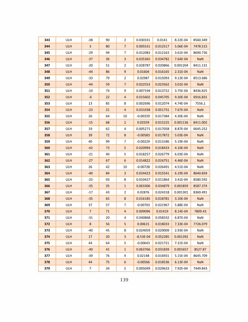
139
343 ULH -38 90 2 0.030331 0.0141 8.22E-04 8560.349
344 ULH 3 80 7 0.005531 0.012517 5.06E-04 7478.515
345 ULH -29 94 7 0.012083 0.012163 3.61E-04 8690.736
346 ULH -37 36 3 0.035365 0.034782 7.64E-04 NaN
347 ULH -20 51 2 0.028787 0.020866 0.001204 8411.131
348 ULH -44 86 9 0.01604 0.016165 2.31E-04 NaN
349 ULH -33 79 2 0.02987 0.015093 9.13E-04 8513.686
350 ULH -44 59 7 0.022553 0.023562 3.01E-04 NaN
351 ULH -10 74 9 0.007194 0.013722 3.75E-04 8436.825
352 ULH -6 22 4 0.015602 0.045705 9.20E-04 6916.831
353 ULH 13 85 8 0.002696 0.012074 4.74E-04 7556.1
354 ULH -23 21 4 0.031038 0.051731 7.67E-04 NaN
355 ULH 26 64 10 -0.00329 0.017384 4.30E-04 NaN
356 ULH -15 68 2 0.02559 0.015225 0.001136 8411.002
357 ULH 19 62 4 0.005271 0.017058 8.87E-04 6645.252
358 ULH 39 72 8 -0.00583 0.017872 5.03E-04 NaN
359 ULH 40 99 7 -0.00229 0.013186 5.19E-04 NaN
360 ULH -42 73 5 0.020994 0.018433 4.10E-04 NaN
361 ULH -21 40 5 0.018257 0.026779 6.03E-04 NaN
362 ULH -27 67 6 0.014822 0.016751 4.46E-04 NaN
363 ULH 26 42 10 -0.00728 0.026491 4.51E-04 NaN
364 ULH -40 84 3 0.024423 0.015541 6.19E-04 8640.834
365 ULH -25 93 8 0.010427 0.011864 3.41E-04 8580.592
366 ULH -35 35 1 0.063306 0.034879 0.001859 8587.374
367 ULH -17 43 2 0.02876 0.024318 0.001301 8369.491
368 ULH -35 65 8 0.016185 0.018781 3.10E-04 NaN
369 ULH 37 57 7 -0.00703 0.021967 5.88E-04 NaN
370 ULH 7 71 4 0.009096 0.01419 8.14E-04 7809.43
371 ULH -31 20 4 0.040868 0.058332 6.87E-04 NaN
372 ULH 8 56 5 0.00615 0.018033 7.33E-04 7726.079
373 ULH -40 45 8 0.024059 0.029009 2.93E-04 NaN
374 ULH 17 20 3 -8.53E-04 0.052285 0.001392 NaN
375 ULH 44 64 5 -0.00643 0.021721 7.31E-04 NaN
376 ULH -40 41 1 0.063766 0.031839 0.001657 8527.87
377 ULH -39 76 4 0.02148 0.016931 5.15E-04 8645.709
378 ULH 44 75 6 -0.00566 0.018536 6.13E-04 NaN
379 ULH 7 34 5 0.005049 0.029633 7.92E-04 7449.843
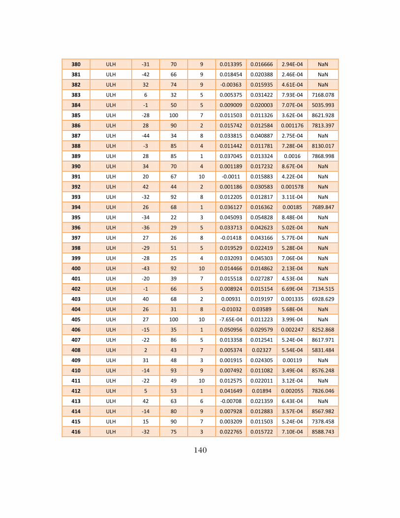
140
380 ULH -31 70 9 0.013395 0.016666 2.94E-04 NaN
381 ULH -42 66 9 0.018454 0.020388 2.46E-04 NaN
382 ULH 32 74 9 -0.00363 0.015935 4.61E-04 NaN
383 ULH 6 32 5 0.005375 0.031422 7.93E-04 7168.078
384 ULH -1 50 5 0.009009 0.020003 7.07E-04 5035.993
385 ULH -28 100 7 0.011503 0.011326 3.62E-04 8621.928
386 ULH 28 90 2 0.015742 0.012584 0.001176 7813.397
387 ULH -44 34 8 0.033815 0.040887 2.75E-04 NaN
388 ULH -3 85 4 0.011442 0.011781 7.28E-04 8130.017
389 ULH 28 85 1 0.037045 0.013324 0.0016 7868.998
390 ULH 34 70 4 0.001189 0.017232 8.67E-04 NaN
391 ULH 20 67 10 -0.0011 0.015883 4.22E-04 NaN
392 ULH 42 44 2 0.001186 0.030583 0.001578 NaN
393 ULH -32 92 8 0.012205 0.012817 3.11E-04 NaN
394 ULH 26 68 1 0.036127 0.016362 0.00185 7689.847
395 ULH -34 22 3 0.045093 0.054828 8.48E-04 NaN
396 ULH -36 29 5 0.033713 0.042623 5.02E-04 NaN
397 ULH 27 26 8 -0.01418 0.043166 5.77E-04 NaN
398 ULH -29 51 5 0.019529 0.022419 5.28E-04 NaN
399 ULH -28 25 4 0.032093 0.045303 7.06E-04 NaN
400 ULH -43 92 10 0.014466 0.014862 2.13E-04 NaN
401 ULH -20 39 7 0.015518 0.027287 4.53E-04 NaN
402 ULH -1 66 5 0.008924 0.015154 6.69E-04 7134.515
403 ULH 40 68 2 0.00931 0.019197 0.001335 6928.629
404 ULH 26 31 8 -0.01032 0.03589 5.68E-04 NaN
405 ULH 27 100 10 -7.65E-04 0.011223 3.99E-04 NaN
406 ULH -15 35 1 0.050956 0.029579 0.002247 8252.868
407 ULH -22 86 5 0.013358 0.012541 5.24E-04 8617.971
408 ULH 2 43 7 0.005374 0.02327 5.54E-04 5831.484
409 ULH 31 48 3 0.001915 0.024305 0.00119 NaN
410 ULH -14 93 9 0.007492 0.011082 3.49E-04 8576.248
411 ULH -22 49 10 0.012575 0.022011 3.12E-04 NaN
412 ULH 5 53 1 0.041649 0.01894 0.002055 7826.046
413 ULH 42 63 6 -0.00708 0.021359 6.43E-04 NaN
414 ULH -14 80 9 0.007928 0.012883 3.57E-04 8567.982
415 ULH 15 90 7 0.003209 0.011503 5.24E-04 7378.458
416 ULH -32 75 3 0.022765 0.015722 7.10E-04 8588.743

141
417 ULH 38 91 6 -0.00137 0.013945 5.98E-04 NaN
418 ULH -26 80 5 0.014757 0.013908 5.09E-04 8586.369
419 ULH 42 81 4 -2.91E-04 0.016613 8.12E-04 NaN
420 ULH -26 94 3 0.019622 0.011836 7.09E-04 8558.437
421 ULH 16 83 9 0.001356 0.012534 4.39E-04 NaN
422 ULH 18 72 7 0.001673 0.014604 5.56E-04 NaN
423 ULH -2 64 5 0.009206 0.015635 6.69E-04 7531.981
424 ULH 11 45 5 0.00434 0.022638 7.76E-04 7540.564
425 ULH 4 51 3 0.013062 0.019656 0.001081 7944.072
426 ULH -14 96 9 0.007408 0.010736 3.47E-04 8548.803
427 ULH 18 49 10 -0.0023 0.021458 4.35E-04 NaN
428 ULH 1 51 10 0.003988 0.019611 3.93E-04 5380.585
429 ULH 8 28 6 0.002197 0.036065 6.94E-04 6865.381
430 ULH 33 74 4 0.002049 0.016113 8.54E-04 8350.491
431 ULH 43 67 4 -0.00309 0.020408 8.57E-04 NaN
432 ULH -16 24 6 0.019164 0.043346 5.68E-04 NaN
433 ULH 28 72 4 0.00344 0.01573 8.62E-04 6943.611
434 ULH 22 23 4 -0.00674 0.046893 0.001081 NaN
435 ULH -30 63 5 0.017824 0.018329 5.05E-04 NaN
436 ULH -6 42 1 0.045802 0.023941 0.002201 7909.59
437 ULH 33 27 3 -0.00962 0.044162 0.001358 NaN
438 ULH 2 63 10 0.003776 0.015883 3.87E-04 5691.566
439 ULH -11 81 2 0.02405 0.012577 0.001086 8203.937
440 ULH -4 51 6 0.008588 0.019656 5.91E-04 7316.07
441 ULH 7 61 5 0.006647 0.016517 7.16E-04 7873.588
442 ULH -18 50 5 0.015158 0.021029 6.05E-04 8648.067
443 ULH -41 60 4 0.025313 0.022084 5.19E-04 NaN
444 ULH -5 38 8 0.007715 0.026416 4.70E-04 5318.699
445 ULH -36 63 5 0.020192 0.01962 4.63E-04 NaN
446 ULH -12 87 8 0.007856 0.011751 3.97E-04 8538.358
447 ULH 1 54 4 0.010502 0.018521 8.43E-04 7282.555
448 ULH -23 26 2 0.037976 0.041783 0.00137 8546.933
449 ULH -29 43 9 0.017702 0.02659 3.16E-04 NaN
450 ULH -37 82 1 0.05249 0.01527 0.001272 8415.669
451 ULH -8 56 9 0.007321 0.018033 3.96E-04 7835.966
452 ULH -3 62 7 0.007031 0.016151 5.07E-04 6374.564
453 ULH 14 66 10 5.52E-04 0.015615 4.13E-04 NaN
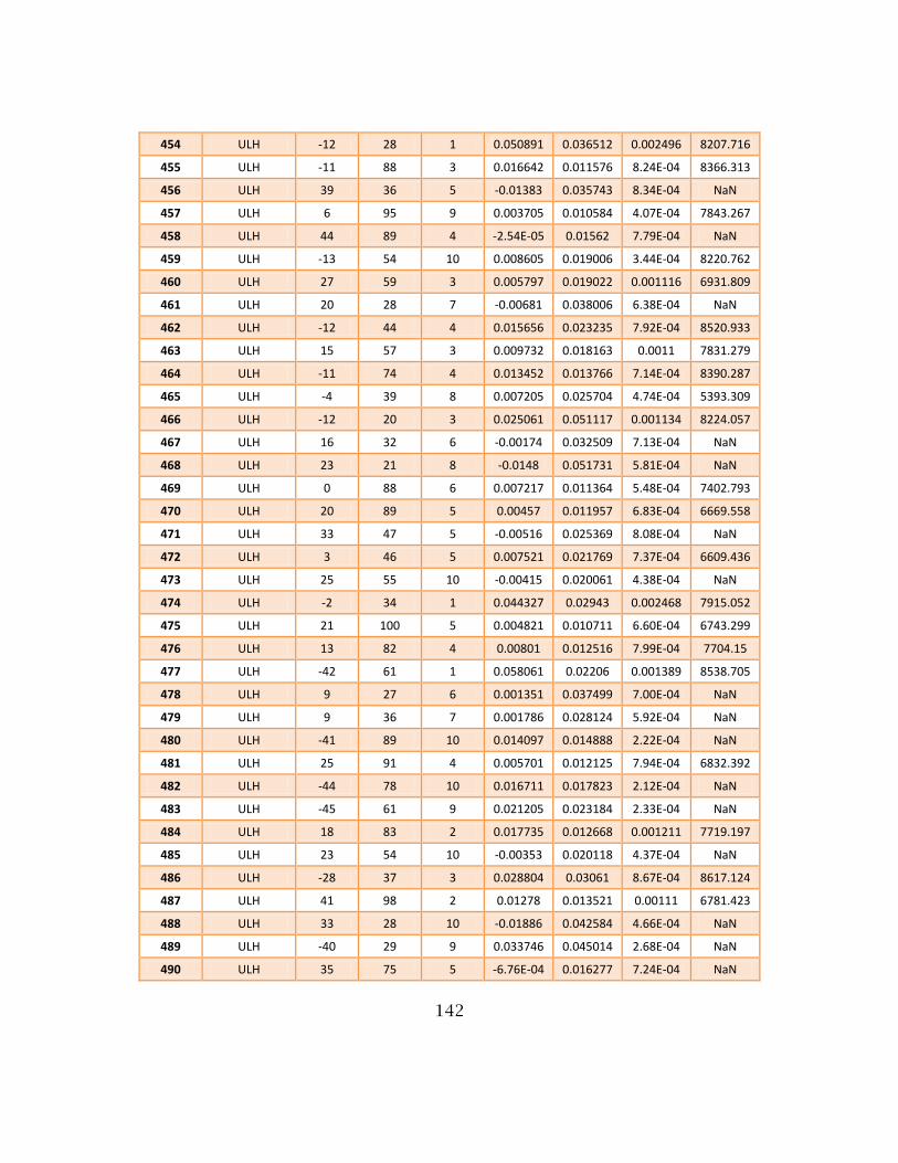
142
454 ULH -12 28 1 0.050891 0.036512 0.002496 8207.716
455 ULH -11 88 3 0.016642 0.011576 8.24E-04 8366.313
456 ULH 39 36 5 -0.01383 0.035743 8.34E-04 NaN
457 ULH 6 95 9 0.003705 0.010584 4.07E-04 7843.267
458 ULH 44 89 4 -2.54E-05 0.01562 7.79E-04 NaN
459 ULH -13 54 10 0.008605 0.019006 3.44E-04 8220.762
460 ULH 27 59 3 0.005797 0.019022 0.001116 6931.809
461 ULH 20 28 7 -0.00681 0.038006 6.38E-04 NaN
462 ULH -12 44 4 0.015656 0.023235 7.92E-04 8520.933
463 ULH 15 57 3 0.009732 0.018163 0.0011 7831.279
464 ULH -11 74 4 0.013452 0.013766 7.14E-04 8390.287
465 ULH -4 39 8 0.007205 0.025704 4.74E-04 5393.309
466 ULH -12 20 3 0.025061 0.051117 0.001134 8224.057
467 ULH 16 32 6 -0.00174 0.032509 7.13E-04 NaN
468 ULH 23 21 8 -0.0148 0.051731 5.81E-04 NaN
469 ULH 0 88 6 0.007217 0.011364 5.48E-04 7402.793
470 ULH 20 89 5 0.00457 0.011957 6.83E-04 6669.558
471 ULH 33 47 5 -0.00516 0.025369 8.08E-04 NaN
472 ULH 3 46 5 0.007521 0.021769 7.37E-04 6609.436
473 ULH 25 55 10 -0.00415 0.020061 4.38E-04 NaN
474 ULH -2 34 1 0.044327 0.02943 0.002468 7915.052
475 ULH 21 100 5 0.004821 0.010711 6.60E-04 6743.299
476 ULH 13 82 4 0.00801 0.012516 7.99E-04 7704.15
477 ULH -42 61 1 0.058061 0.02206 0.001389 8538.705
478 ULH 9 27 6 0.001351 0.037499 7.00E-04 NaN
479 ULH 9 36 7 0.001786 0.028124 5.92E-04 NaN
480 ULH -41 89 10 0.014097 0.014888 2.22E-04 NaN
481 ULH 25 91 4 0.005701 0.012125 7.94E-04 6832.392
482 ULH -44 78 10 0.016711 0.017823 2.12E-04 NaN
483 ULH -45 61 9 0.021205 0.023184 2.33E-04 NaN
484 ULH 18 83 2 0.017735 0.012668 0.001211 7719.197
485 ULH 23 54 10 -0.00353 0.020118 4.37E-04 NaN
486 ULH -28 37 3 0.028804 0.03061 8.67E-04 8617.124
487 ULH 41 98 2 0.01278 0.013521 0.00111 6781.423
488 ULH 33 28 10 -0.01886 0.042584 4.66E-04 NaN
489 ULH -40 29 9 0.033746 0.045014 2.68E-04 NaN
490 ULH 35 75 5 -6.76E-04 0.016277 7.24E-04 NaN

143
491 ULH -41 79 9 0.015815 0.016772 2.47E-04 NaN
492 ULH -14 30 3 0.022744 0.034354 0.001052 8552.721
493 ULH 41 23 4 -0.02697 0.057609 0.001067 NaN
494 ULH 17 90 9 0.001414 0.011619 4.34E-04 NaN
495 ULH 34 25 1 0.01632 0.048249 0.00307 6914.832
496 ULH 0 62 6 0.007217 0.016129 5.90E-04 5109.641
497 ULH 3 28 2 0.019778 0.035763 0.001694 7796.367
498 ULH 11 97 10 0.002326 0.010502 3.83E-04 7580.816
499 ULH 13 53 10 -2.60E-05 0.019364 4.22E-04 NaN
Recommended