i
DESIGN AND PERFORMANCE ANALYSIS OF FAULT TOLERANT TTCAN SYSTEMS
by
AAKASH ARORA
THESIS
Submitted to the Graduate School
of Wayne State University,
Detroit, Michigan
in partial fulfillment of the requirements
for the degree of
MASTER OF SCIENCE
August 2005
MAJOR: COMPUTER ENGINEERING
Approved by:
Advisor Date
i
2
TABLE OF CONTENTS
ACKNOWLEDGEMENTS…………………………………………………….…...... i
LIST OF TABLES…………………………………………………………………….. iv
LIST OF FIGURES…………………………………………………………………… v
1 INTRODUCTION…………………………………………………………………… 1
2 LITERATURE REVIEW……………………………………………………………. 6
2.1 Fault Tolerance Theory…………………………………………………… 6
2.1.1 Classification of failures …………………………………………7
2.1.2 Classification of Failures in CAN and TTCAN........................ 7
2.2 Error Rate in TTCAN……………………………………………………… 8
2.3 Introducing Fault Tolerance in TTCAN………………………………….. 9
3 PROPOSED FAULT TOLERANCE TECHNIQUES FOR TTCAN……………13
3.1 Assumptions……………………………………………………………….13
3.2 Mailbox Method……………………………………………………………14
3.2.1 Proposed Architecture………………………………………….14
3.2.2 Algorithm…………………………………………………………15
3.2.3 Analysis…………………………………………………………..18
3.3 Arbitration Window Method………………………………………………20
3.3.1 Proposed Architecture………………………………………….21
3.3.2 Algorithm…………………………………………………………22
3.3.3 Analysis…………………………………………………………..24
3.4 Asynchronous Redundant Bus Method…………………………………25
3.4.1 Proposed Architecture………………………………………….26
2
3
3.4.2 Algorithm…………………………………………………………27
3.4.3 Analysis…………………………………………………………..29
4 PERFORMANCE ANALYSIS……………………………………………………..32
4.1 Performance Analysis of Mailbox Method……………………………...32
4.1.1 Results …………………………………………………………..32
4.1.2 Analysis………………………………………………………….36
4.2 Performance Analysis of Arbitration Window Method………………...38
4.2.1 Results …………………………………………………………..38
4.2.2 Analysis………………………………………………………….40
4.3 Performance Analysis of Asynchronous Redundant Bus Method…..41
4.3.1 Results…………………………………………………………...42
4.3.2 Analysis…………………………………………………………..44
4.4 Comparison of Proposed Techniques ………………………………… 46
5 CONCLUSION………………………………………………………………………48
6 FUTURE WORK……………………………………………………………………50
REFERENCES……………………………………………………………………….. 51
ABSTRACT…………………………………………………………………………….54
AUTOBIOGRAPHICAL STATEMENT……………………………………………...56
3
4
LIST OF TABLES
Table I: Bit error rates………………………………………………………………….8
Table II: Testing environment………………………………………………………...9
Table III: Failures per hour…………………………………………………………...9
Table IV: Delay in the case of Mailbox Window Method………………………….36
Table V: Delay in case of Arbitration Window Method ……………………………40
Table VI: Number of messages per hour missing deadline………………………43
Table VII: Comparison of Worst Case Delay……………………………………….46
Table VIII: Comparison of probability of unsuccessful delivery…………………..47
4
5
LIST OF FIGURES
Figure 1: Progression of application of electronics in vehicles……………………..1
Figure 2: TTCAN System Matrix ……………………………………………………...3
Figure 3: Safety critical applications of in-vehicle networks………………………..4
Figure 4: Proposed System Architecture……………………………………………15
Figure 5: A System Matrix with a Mailbox Window in every basic cycle………...16
Figure 6: Proposed Algorithm for Mailbox window Method……………………….17
Figure 7: A TTCAN System Matrix for the Arbitration Window Method………….22
Figure 8: Algorithm for Proposed Arbitration Window method……………………23
Figure 9: TTCAN system with redundant bus………………………………………26
Figure 10: Proposed TTCAN architecture with asynchronous redundant bus….27
Figure 11: Algorithm for Proposed Asynchronous Redundant Bus method…….28
Figure 12: Calculation of delay……………………………………………………….29
Figure 13: Effect of mailbox window…………………………………………………33
Figure 14: Effect of number of time windows in a basic cycle…………………....34
Figure 15: Effect of average failure rate per second (λ )………………………....35
Figure 16: Effect of Arbitration Window method…………………………………...39
Figure 17: Effect of average failure rate per second ……………………………...39
Figure 18: Average latency versus Secondary bus speed……………………….43
Figure 19: Effect of Asynchronous Redundant Bus Technique……………….....44
5
1
1 INTRODUCTION
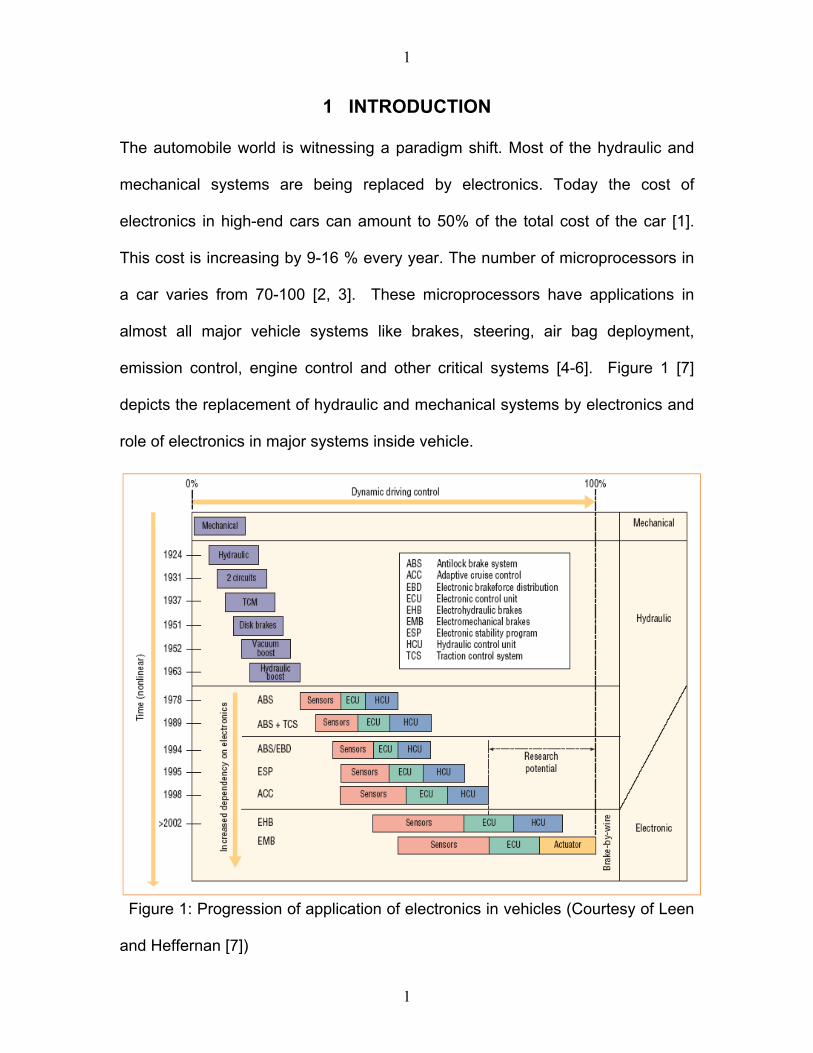
The automobile world is witnessing a paradigm shift. Most of the hydraulic and
mechanical systems are being replaced by electronics. Today the cost of
electronics in high-end cars can amount to 50% of the total cost of the car [1].
This cost is increasing by 9-16 % every year. The number of microprocessors in
a car varies from 70-100 [2, 3]. These microprocessors have applications in
almost all major vehicle systems like brakes, steering, air bag deployment,
emission control, engine control and other critical systems [4-6]. Figure 1 [7]
depicts the replacement of hydraulic and mechanical systems by electronics and
role of electronics in major systems inside vehicle.
Figure 1: Progression of application of electronics in vehicles (Courtesy of Leen
and Heffernan [7])
1
2
In order to be effective, sensors, actuators and microprocessors in a vehicle must
communicate using appropriate network protocols. A fine comparison of 40 such
protocols that exist since early 1980’s can be found in [7], [8] and [9]. By far CAN
(Controller Area Network) has been the most dominating protocol in Europe and
is now being used in the USA as well. The fact that last year almost 300 million
CAN microchips were sold [10], establishes the worldwide acceptance of CAN.
CAN was invented by Robert Bosch in the1980’s. The basic features of CAN like
high speed serial interface, low cost physical medium, short data lengths, fast
reaction times, multi-master and peer-to-peer communication, error detection and
containment [11] make it the common choice for many designers.
Factors like cost, stability, reliability and safety demand a distributed, safety
critical real-time computing platform [3]. But the event-triggered nature of CAN
prevents it from being used for deterministic real-time communications. Message
latency is not guaranteed in CAN and increases with higher bus message traffic
load [7]. This pushed research on time-based scheduling of messages for in-
vehicle networks in the early 1990’s. As a result, various time-triggered
architectures started to emerge. One of these, TTCAN, is based on unchanged
standard of CAN protocol [12].
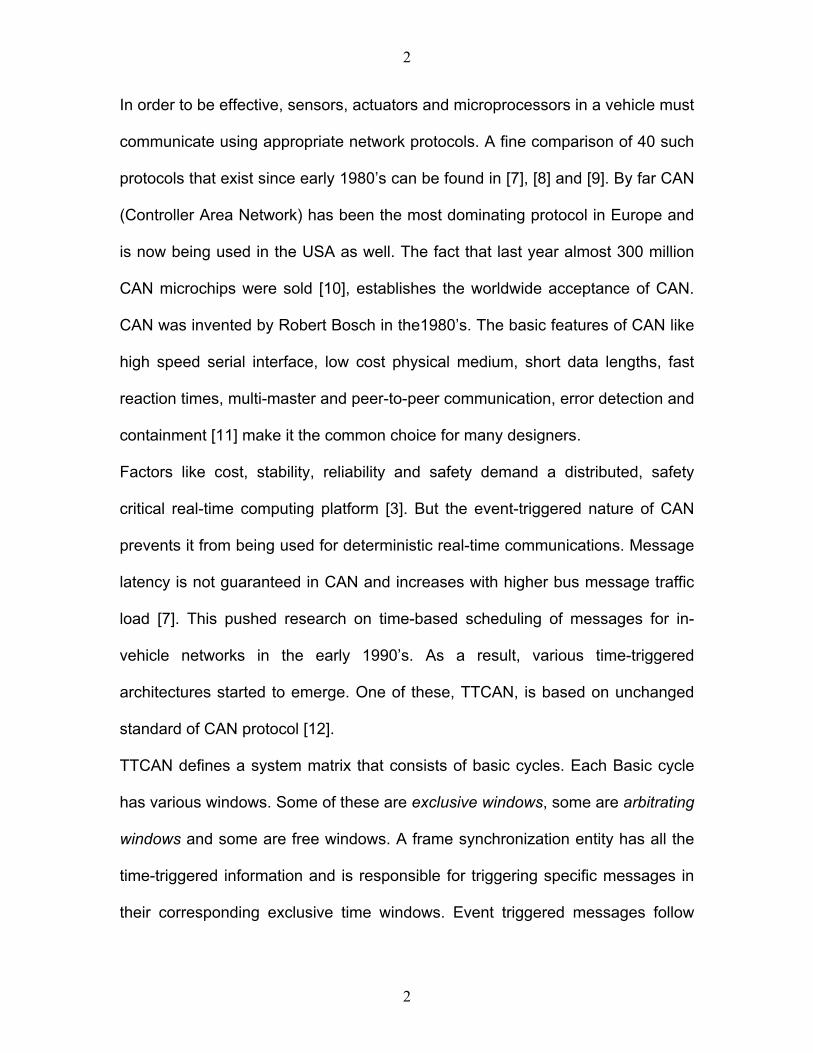
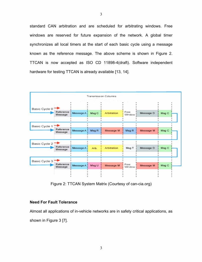
TTCAN defines a system matrix that consists of basic cycles. Each Basic cycle
has various windows. Some of these are exclusive windows, some are arbitrating
windows and some are free windows. A frame synchronization entity has all the
time-triggered information and is responsible for triggering specific messages in
their corresponding exclusive time windows. Event triggered messages follow
2
3
standard CAN arbitration and are scheduled for arbitrating windows. Free
windows are reserved for future expansion of the network. A global timer
synchronizes all local timers at the start of each basic cycle using a message
known as the reference message. The above scheme is shown in Figure 2.
TTCAN is now accepted as ISO CD 11898-4(draft). Software independent
hardware for testing TTCAN is already available [13, 14].
Figure 2: TTCAN System Matrix (Courtesy of can-cia.org)
Need For Fault Tolerance
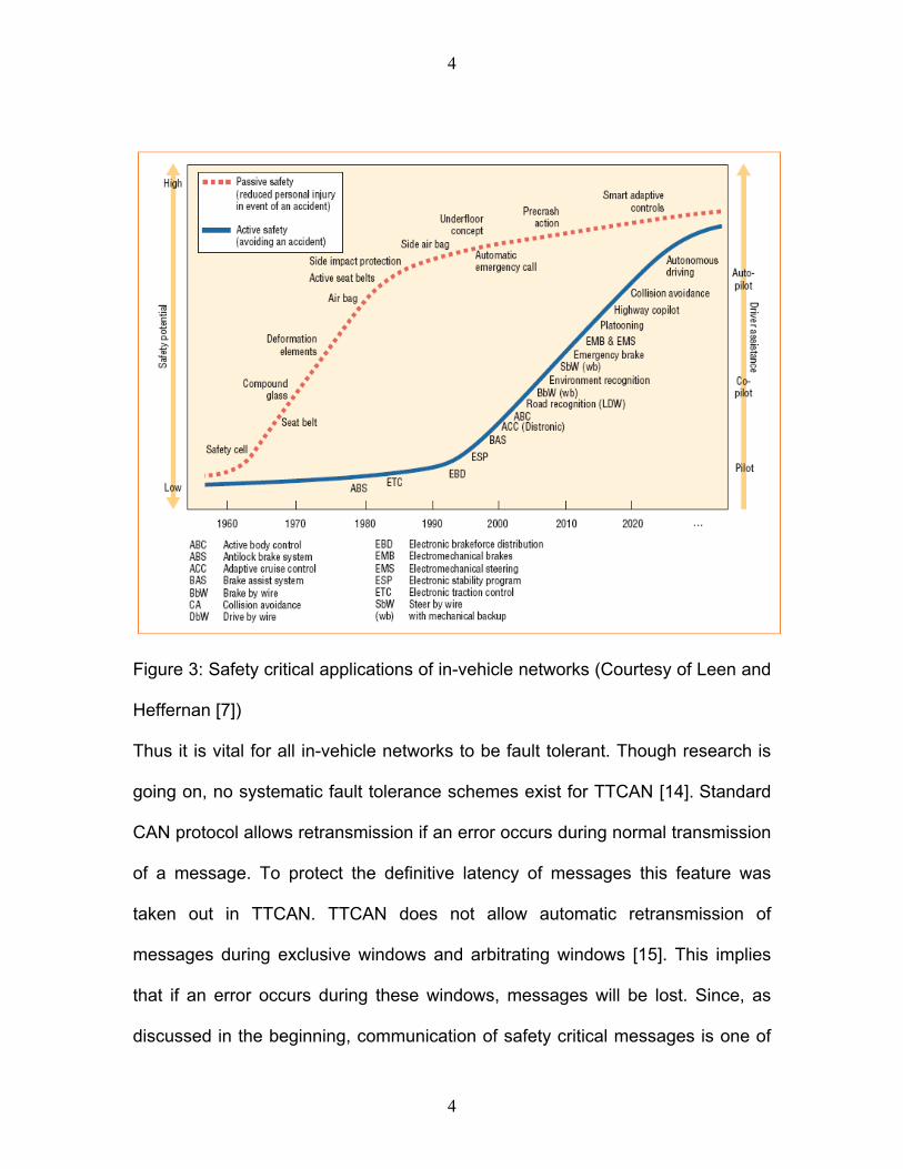
Almost all applications of in-vehicle networks are in safety critical applications, as
shown in Figure 3 [7].
3
4
Figure 3: Safety critical applications of in-vehicle networks (Courtesy of Leen and
Heffernan [7])
Thus it is vital for all in-vehicle networks to be fault tolerant. Though research is
going on, no systematic fault tolerance schemes exist for TTCAN [14]. Standard
CAN protocol allows retransmission if an error occurs during normal transmission
of a message. To protect the definitive latency of messages this feature was
taken out in TTCAN. TTCAN does not allow automatic retransmission of
messages during exclusive windows and arbitrating windows [15]. This implies
that if an error occurs during these windows, messages will be lost. Since, as
discussed in the beginning, communication of safety critical messages is one of
4
5
the main purposes of using TTCAN, loss of these messages defeats the purpose
of this new protocol, and much more than that puts the life of passengers at risk.
A study [16] shows that it is possible to have up to 2480 failures per hour in a
TTCAN system in the worst case. Hence to protect the lives of passengers, it is
important to make TTCAN completely fault tolerant. The main objective of the
thesis work presented here is to increase the fault tolerance of the TTCAN
systems by addressing the above mentioned issue. The work presented here
makes an attempt to achieve this goal by proposing and analyzing three new
techniques for increasing fault tolerance. The first two techniques ameliorate the
design of the system matrix to reduce the probability of unsuccessful delivery of a
message. These methods have been discussed analytically. The third technique
describes a method of incorporating an asynchronous redundant bus. This
method has been analyzed using simulations.
The work has been organized as following. Chapter 2 presents a survey of
existing literature on fault tolerance in time-triggered protocols, focusing on Time
Triggered CAN. Chapter 3 describes the proposed schemes for increasing fault
tolerance in TTCAN. It goes on to discuss the required architectures and
algorithms for successful implementation of these methods. Also various
parameters like worst-case response time, latency, average rate of failure per
second, etc that are used for analysis and simulation, are described in this
chapter. Parameters like probability of unsuccessful delivery and delay in delivery
of a message facing error are studied. Chapter 5 presents the conclusion and
Chapter 6 presents the future work.
5
6
2 Literature Review
2.1 Fault Tolerance Theory
Fault tolerance is defined as the ability of a system to respond gracefully to an
unexpected hardware or software failure. According to another definition, it is the
ability of a system or a component to continue normal operation despite the
presence of faults.
In case of X-by-wire systems, the definition and theory of fault tolerance provided
by Cedric Wilwert, et al in [17] is most suited. The paper defines fault tolerance
as a means of dependability, as much as fault prevision, fault prevention and
fault elimination. The authors go on further to distinguish and define errors, faults
and failures. As per their definition,
• Failure is a condition when the service delivered deviates from the
specified service. The failure is also the effect of an error on the service.
• Error is the part of the state of system which is susceptible to produce a
failure, and this is also the manifestation of a fault in the system.
• Fault is the supposed or assumed cause of an error.
The “fault-error-failure” chain is recursive, i.e., fault in a system will lead to an
error which will result in a failure. This failure will become a fault of some other
systems and the chain will continue. A nice example is of coding failure caused
by reasoning errors. This failure becomes a dormant fault in software. When
activated, this fault will lead to errors in data being processed by software. The
output will deviate from the expected outcome, thus causing failure.
6
7
The aim of fault tolerance is to provide means for graceful degradation of a
system in a manner that deviation of actual output from expected output is
minimum possible.
2.1.1 Classification of failures
For analyzing fault tolerance of a system it is necessary to have a failure model
for the system. Failures can be defined in different dimensions [17]. Two such
basic dimensions are value domain and temporal domain.
In the value domain, failures can be categorized as Byzantine failures, Coherent
failures and Fail-Silent failures. The Byzantine failure occurs when a failure is
perceived differently in non faulty nodes of the network. If all nodes perceive the
failure identically then the failure is known as Coherent failure. If no
communication is received by the nodes when they expect to receive it, the
failure is known as Fail-silent.
In the temporal domain, failures are categorized as permanent failures, transient
failures and intermittent. If the failure is irreparable then it is known as Permanent
failure. Transient failures are caused by external and transient stimulus.
Intermittent failures are caused by conception faults that are repeated
intermittently.
2.1.2 Classification of Failures in CAN and TTCAN Systems
Most of the fault tolerance studies for in-vehicle networks have been done on
coherent or fail salient transient failure models. Some studies [18, 16] categorize
7
8
the failures in a CAN system as Inconsistent Message Duplicate (IMD) failures
and Inconsistent Message Omission (IMO) failures.
In a CAN system, sometimes nodes may receive the same message twice, this is
called Inconsistent Message Duplicate (IMD) failure whereas in some other
cases, nodes may not receive a message, this is known as Inconsistent Message
Omission (IMO) failure. As discussed in Chapter 1, in a TTCAN system
retransmission of a message is not allowed in case of an error. Thus, in a
TTCAN system we only have IMO failures.
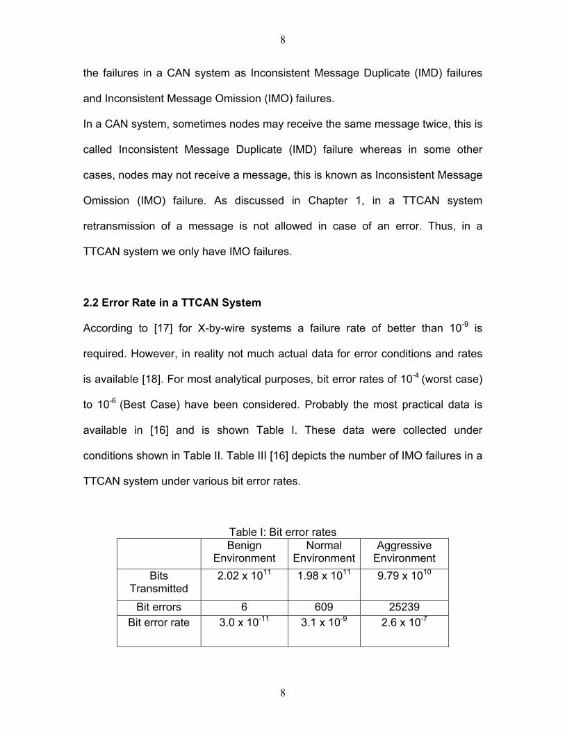
2.2 Error Rate in a TTCAN System According to [17] for X-by-wire systems a failure rate of better than 10-9 is
required. However, in reality not much actual data for error conditions and rates
is available [18]. For most analytical purposes, bit error rates of 10-4 (worst case)
to 10-6 (Best Case) have been considered. Probably the most practical data is
available in [16] and is shown Table I. These data were collected under
conditions shown in Table II. Table III [16] depicts the number of IMO failures in a
TTCAN system under various bit error rates.
Table I: Bit error rates Benign
Environment Normal
EnvironmentAggressive
Environment Bits
Transmitted 2.02 x 10¹¹ 1.98 x 10¹¹ 9.79 x 10¹⁰
Bit errors 6 609 25239 Bit error rate 3.0 x 10⁻¹¹ 3.1 x 10⁻⁹ 2.6 x 10⁻⁷
8
9
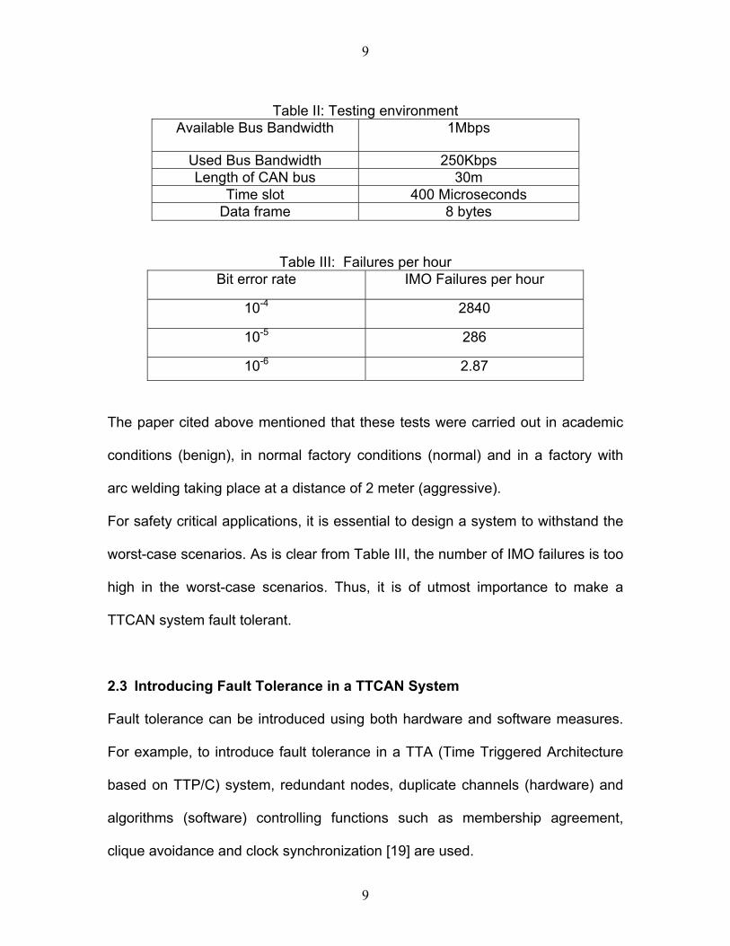
Table II: Testing environment
Available Bus Bandwidth 1Mbps
Used Bus Bandwidth 250Kbps Length of CAN bus 30m
Time slot 400 Microseconds Data frame 8 bytes
Table III: Failures per hour Bit error rate IMO Failures per hour
10-4 2840
10-5 286
10-6 2.87
The paper cited above mentioned that these tests were carried out in academic
conditions (benign), in normal factory conditions (normal) and in a factory with
arc welding taking place at a distance of 2 meter (aggressive).
For safety critical applications, it is essential to design a system to withstand the
worst-case scenarios. As is clear from Table III, the number of IMO failures is too
high in the worst-case scenarios. Thus, it is of utmost importance to make a
TTCAN system fault tolerant.
2.3 Introducing Fault Tolerance in a TTCAN System
Fault tolerance can be introduced using both hardware and software measures.
For example, to introduce fault tolerance in a TTA (Time Triggered Architecture
based on TTP/C) system, redundant nodes, duplicate channels (hardware) and
algorithms (software) controlling functions such as membership agreement,
clique avoidance and clock synchronization [19] are used.
9
10
TTCAN provides fault tolerance for global clock synchronization by providing
potential time master nodes. These nodes can become the time master in an
event of failure of actual time master. Thus, the time synchronous nature of a
TTCAN system is preserved [13, 15, 20]. But other than that, no systematic fault
tolerant scheme exists for a TTCAN system [14]. For example, as described in
the problem statement in Chapter 1, in case of occurrence of an error,
retransmission of a message in not allowed. This leads to loss of safety critical
messages, thus endangering lives of passengers.
Different studies have been carried out to address fault tolerance issues in
TTCAN systems. Mϋller, et al proposed a fault tolerant TTCAN in ref [21]. They
proposed to introduce fault tolerance in a TTCAN system by providing
synchronous redundant channels. These channels vary in number from two to
three. The work focuses mainly on the topologies and synchronization issues.
The authors try to solve problems related to phase synchronization of cycle time,
global time and rate. The main drawback of this technique is that it requires the
redundant bus to be dedicated. This means that the redundant bus cannot be
shared between two networks. This problem is inherent to almost all redundant
bus implementations that are synchronous in nature. Another drawback is that
this solution requires the speed of the redundant bus to be exactly same as that
of the primary bus. Same speed of primary and secondary busses is required to
maintain the synchronous nature of the solution.
Colnarič and Verber [22] proposed to use the redundant bus for sharing of bus
load. In this technique there are multiple timetables in Frame Synchronization
10
11
Entity. Each bus has its own timetable for normal circumstances. In case of a
failure, load of one bus is moved to the other. There exists a separate timetable
for such a condition. The failure is detected using a monitor and diagnostic time
slot. In this slot, the time master polls each bus. If there is no reply from any of
the busses, that bus is assumed to have the failure and the load of that bus is
shifted to the other bus. There are several issues related to this proposed
solution. First, the solution has not been proved by analysis, simulation or
experiments. Second, under normal circumstances the bus utilization is very low.
This is done in order to accommodate the load of the secondary bus in case of a
failure. Also, when load of one bus is transferred to another, some messages are
eliminated from the timetable thus decreasing the overall output.
In another study [23], Broster, et al, have tried to handle the IMO failures. In this
case no redundant bus is used. The solution is software based. They have
proposed a new system matrix for reducing the probability of an unsuccessful
delivery. In the system matrix proposed by them, each exclusive window is
repeated twice and is placed next to each other. First the system is studied with
a normal system matrix and the probability of failure is calculated. Then the
system matrix is redesigned as stated above, i.e., by transmitting each message
twice, one after another. Again probability of a failure is calculated. The analysis
is based on poisson’s fault model. The results of this study show that probability
of an unsuccessful delivery decreases in the second case, i.e., when each
message is transmitted twice. Though the scheme produces good results, it is far
less than efficient. Transmitting every message two times forces the period of
11
12
each message to be more than the case when only single transmission is
required. Increasing the period of any message is not a good idea, especially in
case of safety critical messages.
Though work has been done on defining fault tolerance for Time Triggered CAN
systems, collecting bit error rates, failure rates and introducing techniques to
handle failures, no satisfactory solution exists. Especially, not much work has
been done to address the problem of message omission in case of an error. In
Chapter 3, three schemes are proposed to solve this issue.
12
13
3 PROPOSED FAULT TOLERANCE TECHNIQUES FOR TTCAN
As concluded in Chapter 2, not much work has been done on making TTCAN
networks fault tolerant. Especially, the issue of the loss of messages due to
prohibition of retransmission in exclusive time windows has not been addressed
effectively. This section of the thesis work presents three techniques for
addressing this particular problem. Section 3.1 of this thesis describes the
assumptions for the three proposed techniques. Section 3.2 explains the first
proposed technique, which is referred to as the Mailbox Window method. Section
3.3 describes the second proposed technique, which is known as the Arbitration
Window method. Section 3.4 presents the third proposed technique, which is
called the Asynchronous Redundant Bus method.
3.1 Assumptions
The work presented in this section assumes a coherent (in value domain),
transient (in time domain) failure model. Also it is being assumed that for any
practical fault tolerant system, occasional delivery failures are acceptable and
expected and that hard deadlines cannot be made in any form of electrical
communications that are subject to unpredictable faults [23]. The distribution of
faults is considered to follow Poisson’s distribution. All the system design
analysis presented in the following work is for the worst-case scenarios. Also it is
essential to mention here that TTCAN uses the error detection mechanism
identical to that of the CAN which includes Cyclic Redundancy Check (CRC) and
Acknowledgement field in each message.
13
14
3.2 Mailbox Method
The basic objective of this method is to increase the fault tolerance of a TTCAN
system by decreasing the probability of an unsuccessful delivery of a message
and delay in delivery of the message that is caused by the prohibition of
retransmission in an exclusive window. The Mailbox Window method makes an
attempt to decrease this probability by providing an “extra chance” to the failed
message. This chance is provided by attaching an extra window at end of each
basic cycle called the Mailbox window. Any failed message can be dynamically
rescheduled for either any forthcoming arbitrary window in the current basic cycle
or for the Mailbox window. The proposed architecture, algorithm and analysis are
presented in the following sections.
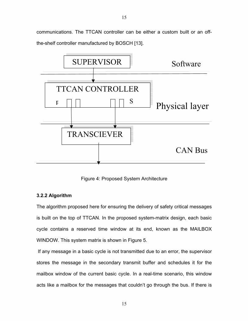
3.2.1 Proposed Architecture The proposed architecture is based on layered network approach. The physical
layer consists of the transceivers and the transfer medium. On the top of this
layer is the TTCAN controller that enforces the protocol. The controller is in turn
supervised by a software layer, which takes care of scheduling and exception
handling algorithms. The TTCAN controller maintains two pairs of receive and
transmit buffers. The transmit buffers are represented by P_Tx_Buf and
S_Tx_Buf. Similarly, the receive buffers are P_Rx_Buf and S_Rx_Buf (where P
and S stand for Primary and Secondary, respectively). Figure 4 shows the above
mentioned architecture.
The physical layer can be implemented using a twisted pair of copper wires.
Available SAE standards for CAN, for example SAEJ2241 etc can be used for
14
15
communications. The TTCAN controller can be either a custom built or an off-
the-shelf controller manufactured by BOSCH [13].
SUPERVISOR Software
TTCAN CONTROLLER SP Physical layer
TRANSCIEVER
CAN Bus
Figure 4: Proposed System Architecture
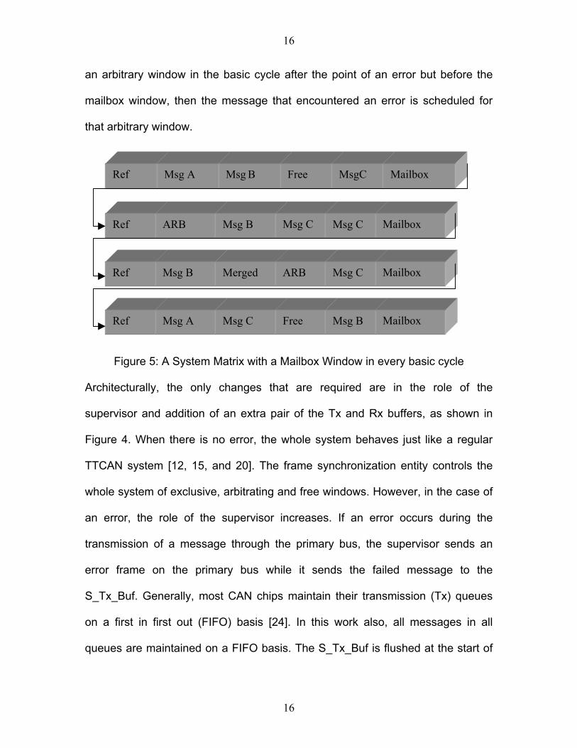
3.2.2 Algorithm The algorithm proposed here for ensuring the delivery of safety critical messages
is built on the top of TTCAN. In the proposed system-matrix design, each basic
cycle contains a reserved time window at its end, known as the MAILBOX
WINDOW. This system matrix is shown in Figure 5.
If any message in a basic cycle is not transmitted due to an error, the supervisor
stores the message in the secondary transmit buffer and schedules it for the
mailbox window of the current basic cycle. In a real-time scenario, this window
acts like a mailbox for the messages that couldn’t go through the bus. If there is
15
16
an arbitrary window in the basic cycle after the point of an error but before the
mailbox window, then the message that encountered an error is scheduled for
that arbitrary window.
Mailbox Msg BFree Msg C Msg A Ref
Mailbox Msg CARB Merged Msg B Ref
Mailbox Msg CMsg CMsg B ARB Ref
Mailbox MsgCFree Msg BMsg A Ref
Figure 5: A System Matrix with a Mailbox Window in every basic cycle
Architecturally, the only changes that are required are in the role of the
supervisor and addition of an extra pair of the Tx and Rx buffers, as shown in
Figure 4. When there is no error, the whole system behaves just like a regular
TTCAN system [12, 15, and 20]. The frame synchronization entity controls the
whole system of exclusive, arbitrating and free windows. However, in the case of
an error, the role of the supervisor increases. If an error occurs during the
transmission of a message through the primary bus, the supervisor sends an
error frame on the primary bus while it sends the failed message to the
S_Tx_Buf. Generally, most CAN chips maintain their transmission (Tx) queues
on a first in first out (FIFO) basis [24]. In this work also, all messages in all
queues are maintained on a FIFO basis. The S_Tx_Buf is flushed at the start of
16
17
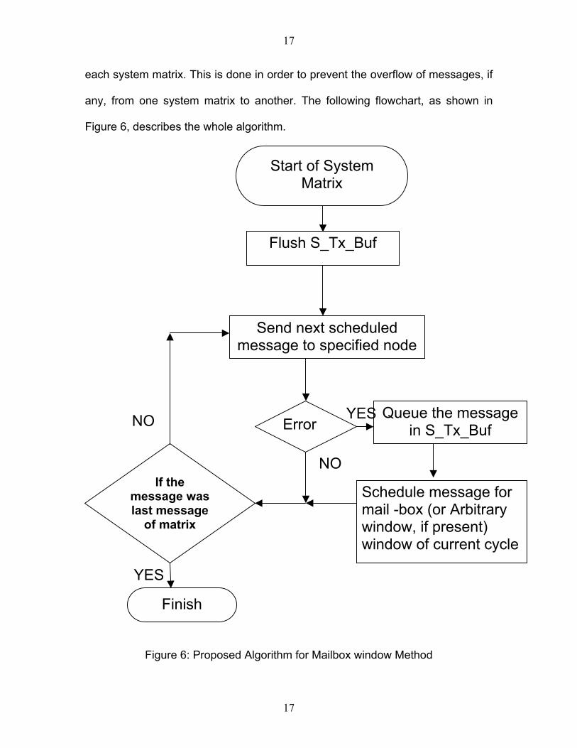
each system matrix. This is done in order to prevent the overflow of messages, if
any, from one system matrix to another. The following flowchart, as shown in
Figure 6, describes the whole algorithm.
Start of System Matrix
Flush S_Tx_Buf
Send next scheduled message to specified node
Queue the message in S_Tx_Buf
YESNO Error
NOIf the
message was last message
of matrix
Schedule message for mail -box (or Arbitrary window, if present) window of current cycle
YES
Finish
Figure 6: Proposed Algorithm for Mailbox window Method
17
18
3.2.3 Analysis
The performance parameters chosen for the proposed scheme are the
probability of unsuccessful delivery and the latency (delay) of message
transmission. The goal of the proposed technique is to reduce the value of both
parameters.
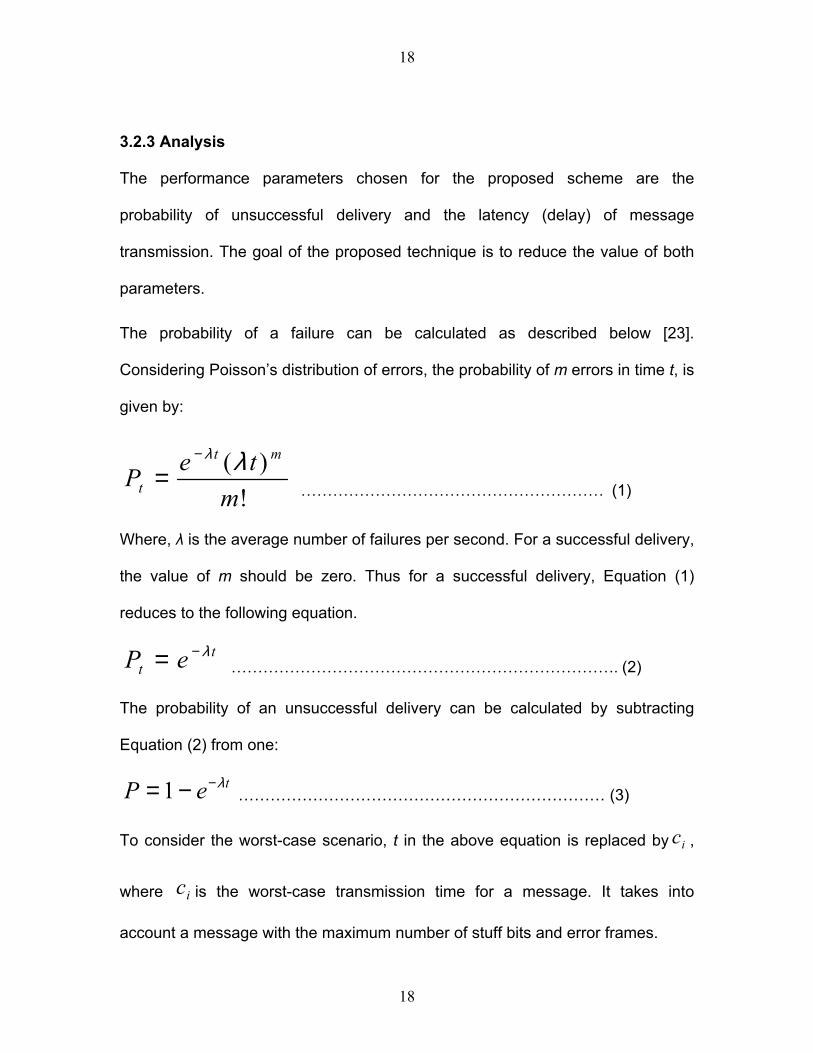
The probability of a failure can be calculated as described below [23].
Considering Poisson’s distribution of errors, the probability of m errors in time t, is
given by:
!)(
mtePmt
tλλ−
= ………………………………………………… (1)
Where, λ is the average number of failures per second. For a successful delivery,
the value of m should be zero. Thus for a successful delivery, Equation (1)
reduces to the following equation.
tt eP λ−= ………………………………………………………………. (2)
The probability of an unsuccessful delivery can be calculated by subtracting
Equation (2) from one:
teP λ−−=1 …………………………………………………………… (3)
To consider the worst-case scenario, t in the above equation is replaced by ,
where is the worst-case transmission time for a message. It takes into
account a message with the maximum number of stuff bits and error frames.
ic
ic
18
19
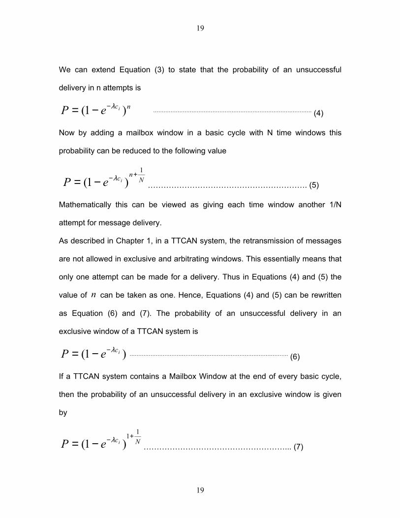
We can extend Equation (3) to state that the probability of an unsuccessful
delivery in n attempts is
ncieP )1( λ−−= ………………………………………………………………………………. (4)
Now by adding a mailbox window in a basic cycle with N time windows this
probability can be reduced to the following value
N
ncieP1
)1(+−−= λ
……………………………………………………. (5)
Mathematically this can be viewed as giving each time window another 1/N
attempt for message delivery.
As described in Chapter 1, in a TTCAN system, the retransmission of messages
are not allowed in exclusive and arbitrating windows. This essentially means that
only one attempt can be made for a delivery. Thus in Equations (4) and (5) the
value of can be taken as one. Hence, Equations (4) and (5) can be rewritten
as Equation (6) and (7). The probability of an unsuccessful delivery in an
exclusive window of a TTCAN system is
n
)1( iceP λ−−= ………………………………………………………………………………. (6)
If a TTCAN system contains a Mailbox Window at the end of every basic cycle,
then the probability of an unsuccessful delivery in an exclusive window is given
by
NcieP11
)1(+−−= λ
………………………………………………... (7)
19
20
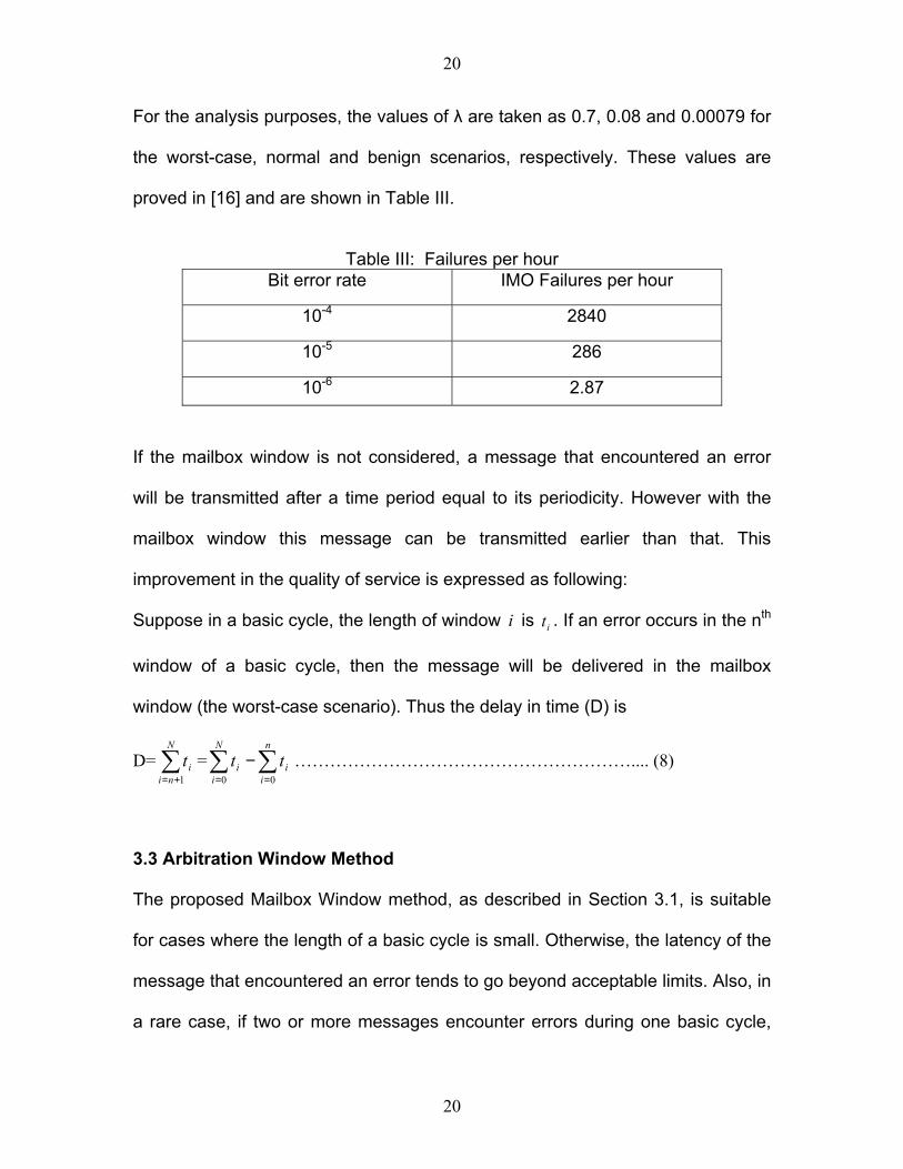
For the analysis purposes, the values of λ are taken as 0.7, 0.08 and 0.00079 for
the worst-case, normal and benign scenarios, respectively. These values are
proved in [16] and are shown in Table III.
Table III: Failures per hour
Bit error rate IMO Failures per hour
10-4 2840
10-5 286
10-6 2.87
If the mailbox window is not considered, a message that encountered an error
will be transmitted after a time period equal to its periodicity. However with the
mailbox window this message can be transmitted earlier than that. This
improvement in the quality of service is expressed as following:
Suppose in a basic cycle, the length of window i is t . If an error occurs in the nith
window of a basic cycle, then the message will be delivered in the mailbox
window (the worst-case scenario). Thus the delay in time (D) is
D= =∑ ………………………………………………….... (8) ∑+=
N
niit
1∑==
−n
ii
N
ii tt
00
3.3 Arbitration Window Method
The proposed Mailbox Window method, as described in Section 3.1, is suitable
for cases where the length of a basic cycle is small. Otherwise, the latency of the
message that encountered an error tends to go beyond acceptable limits. Also, in
a rare case, if two or more messages encounter errors during one basic cycle,
20
21
then only one message is able to make it through the Mailbox Window. To
overcome these shortcomings, a new method is proposed in this section.
As mentioned in Chapter one, a TTCAN system matrix consists of three types of
windows: the exclusive windows, arbitration windows and free windows. The
exclusive windows are reserved for specific messages as per timetable laid out in
frame synchronization entity. The free windows are reserved for future expansion
of the network. The arbitration windows are unreserved. Any message can
compete for the bus during the arbitration window. In case of a collision, as per
CAN specifications, a message with a higher priority wins the bus during the
bitwise arbitration.
The basic idea of the method presented here is to use arbitration windows in a
system matrix design in such a manner that it increases the fault tolerance of the
TTCAN system. It is being assumed that the lowest priority safety critical
message has a higher priority than the highest priority non-safety critical
message. This helps in ensuring that during a collision in an arbitration window,
the safety critical message gets the access to the bus.
3.3.1 Proposed Architecture
The proposed architecture for this technique is identical to the one presented for
the mailbox window method as shown in Figure 4.
21
22
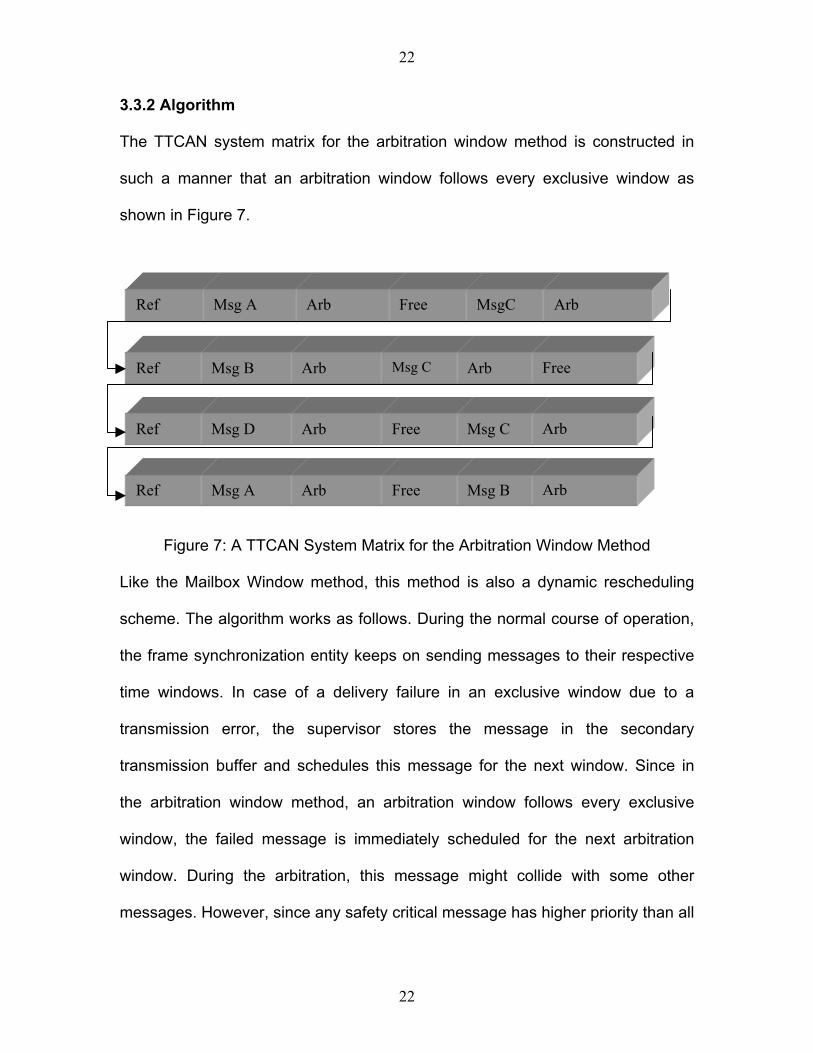
3.3.2 Algorithm
The TTCAN system matrix for the arbitration window method is constructed in
such a manner that an arbitration window follows every exclusive window as
shown in Figure 7.
Arb Msg B Free Arb Msg A Ref
Arb Msg C Free Arb Msg D Ref
Free ArbMsg C Arb Msg B Ref
Arb MsgCFree ArbMsg A Ref
Figure 7: A TTCAN System Matrix for the Arbitration Window Method
Like the Mailbox Window method, this method is also a dynamic rescheduling
scheme. The algorithm works as follows. During the normal course of operation,
the frame synchronization entity keeps on sending messages to their respective
time windows. In case of a delivery failure in an exclusive window due to a
transmission error, the supervisor stores the message in the secondary
transmission buffer and schedules this message for the next window. Since in
the arbitration window method, an arbitration window follows every exclusive
window, the failed message is immediately scheduled for the next arbitration
window. During the arbitration, this message might collide with some other
messages. However, since any safety critical message has higher priority than all
22
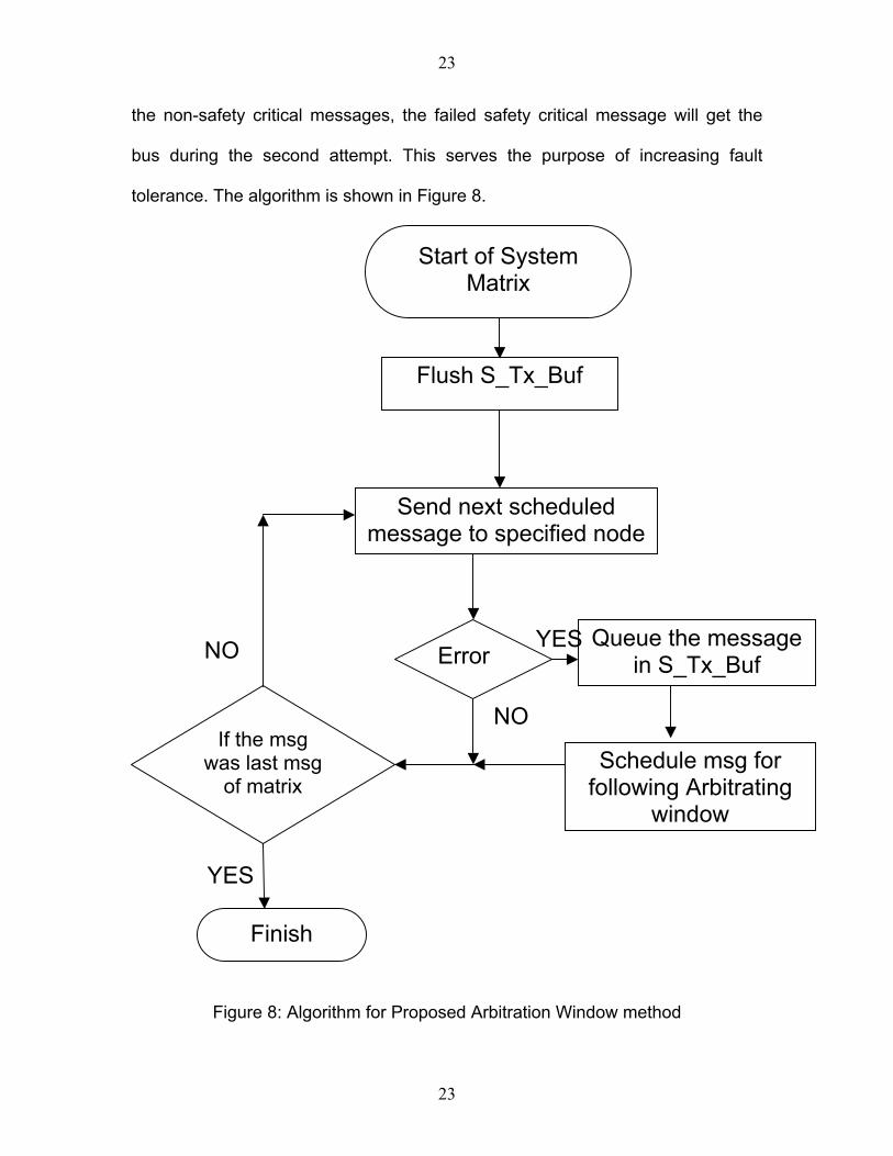
23
the non-safety critical messages, the failed safety critical message will get the
bus during the second attempt. This serves the purpose of increasing fault
tolerance. The algorithm is shown in Figure 8.
Start of System Matrix
Flush S_Tx_Buf
Send next scheduled message to specified node
Queue the message in S_Tx_Buf
YESNO Error
NOIf the msg
was last msg of matrix
Schedule msg for following Arbitrating
window
YES
Finish
Figure 8: Algorithm for Proposed Arbitration Window method
23
24
3.3.3 Analysis
The performance analysis parameters here are the probability of an unsuccessful
delivery and delay in the delivery of the message. The analysis can be extended
from the analysis of the Mailbox Window method. In the Mailbox Window
method, the mailbox window was viewed as providing an extra 1/N (where N is
equal to the number of windows in a basic cycle) chance to the message that
encountered error. In the present case, each message gets one complete (as
compared to 1/N chance in the previous case) extra chance in the form of
arbitrating window that follows its exclusive window. This means that each
message gets two chances of delivery. Thus, for the arbitrary window case,
Equation (7) can be extended to express the probability of an unsuccessful
failure as:
2)1( iceP λ−−= ……………………………………………… (9)
The worst-case delay in this case is equal to the length of longest exclusive
window. This is true because if transmission failure occurs in an exclusive
window the message will get transmitted in the following window which as per
our design is an arbitration window. Hence the transmission will be completed
after a delay of one window length. The length of the longest window can be
calculated as shown below. This calculation has been proved in a study
described in Ref [25]. Also Ref [26] provides an applet to calculate worst case
time for transmission of a CAN message for a given bus speed and data load for
a message.
24
25
bitefsstuff
datastufffixdatafixdata ).tl
1-l ll-l1l(l t +
++++= ……………… (10)
Where
fixl =length of fixed size bits in a message subject to bit stuffing
datal =length of data field
efsl =length of bits which are not subjected to bit stuffing
stuffl = number of stuff bits
bitt =bit timing
Also for error frames
bititerdeflagerror tllt )2( lim+= ……….………………………………………… (11)
Length of a time window in worst case can be calculated by adding (10) and (11).
Delay = errordatawindow ttt += …………………….……………….………..… (12)
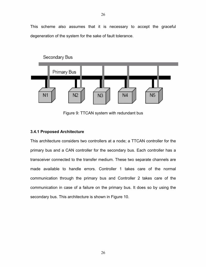
3.4 Asynchronous Redundant Bus Method
In this method a TTCAN system is considered in which a non-synchronous
secondary bus is attached to each node. This arrangement is shown Figure 9. In
the system matrix no mailbox window is considered. The redundant bus need not
be dedicated to a single network. It can be used on a bandwidth sharing basis.
The speed of the redundant bus can differ from the speed of the primary bus.
There is no need of synchronization, i.e., the secondary bus need not have time
slots. The Secondary bus can be a normal CAN bus.
25
26
This scheme also assumes that it is necessary to accept the graceful
degeneration of the system for the sake of fault tolerance.
Figure 9: TTCAN system with redundant bus
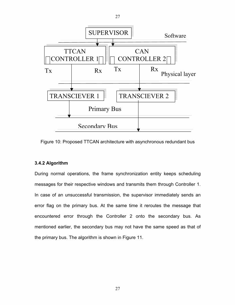
3.4.1 Proposed Architecture
This architecture considers two controllers at a node; a TTCAN controller for the
primary bus and a CAN controller for the secondary bus. Each controller has a
transceiver connected to the transfer medium. These two separate channels are
made available to handle errors. Controller 1 takes care of the normal
communication through the primary bus and Controller 2 takes care of the
communication in case of a failure on the primary bus. It does so by using the
secondary bus. This architecture is shown in Figure 10.
26
27
Figure 10: Proposed TTCAN architecture with asynchronous redundant bus
SUPERVISOR Software
CAN CONTROLLER 2
TTCAN CONTROLLER 1
Tx Rx Tx Rx Physical layer
TRANSCIEVER 2 TRANSCIEVER 1
Primary Bus
Secondary Bus
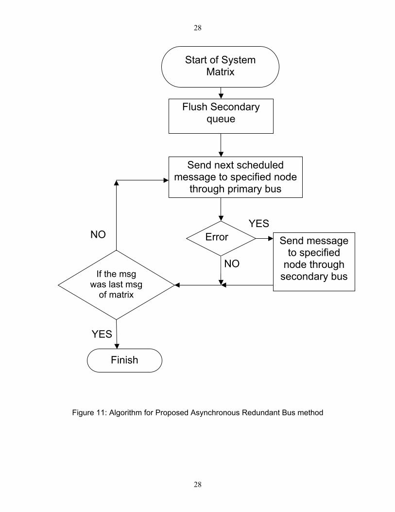
3.4.2 Algorithm
During normal operations, the frame synchronization entity keeps scheduling
messages for their respective windows and transmits them through Controller 1.
In case of an unsuccessful transmission, the supervisor immediately sends an
error flag on the primary bus. At the same time it reroutes the message that
encountered error through the Controller 2 onto the secondary bus. As
mentioned earlier, the secondary bus may not have the same speed as that of
the primary bus. The algorithm is shown in Figure 11.
27
28
Start of System Matrix
Flush Secondary queue
Send message to specified
node through secondary bus
Send next scheduled message to specified node
through primary bus
Error YES
NO
NO
If the msg was last msg
of matrix
YES
Finish
Figure 11: Algorithm for Proposed Asynchronous Redundant Bus method
28
29
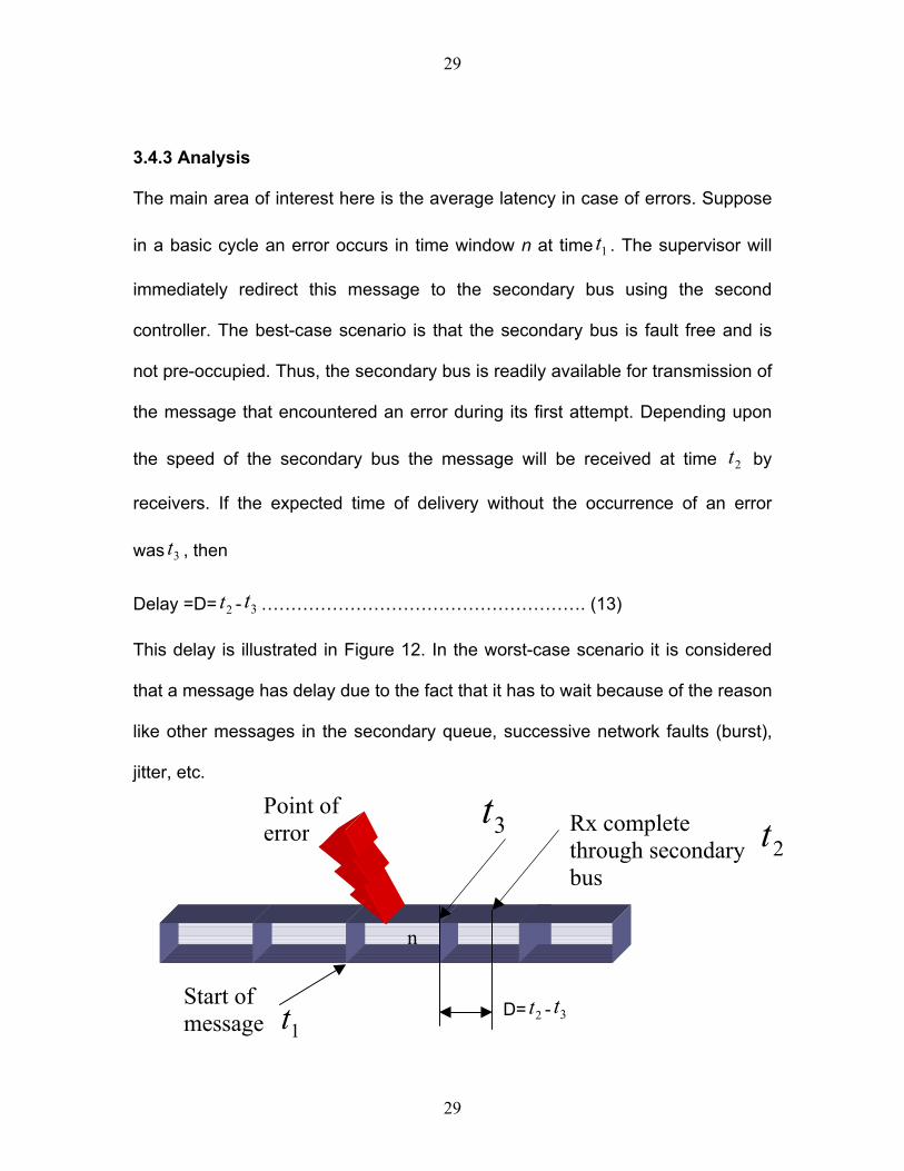
3.4.3 Analysis
The main area of interest here is the average latency in case of errors. Suppose
in a basic cycle an error occurs in time window n at time t . The supervisor will
immediately redirect this message to the secondary bus using the second
controller. The best-case scenario is that the secondary bus is fault free and is
not pre-occupied. Thus, the secondary bus is readily available for transmission of
the message that encountered an error during its first attempt. Depending upon
the speed of the secondary bus the message will be received at time by
receivers. If the expected time of delivery without the occurrence of an error
was t , then
1
2t
3
Delay =D= - ………………………………………………. (13) 2t 3t
This delay is illustrated in Figure 12. In the worst-case scenario it is considered
that a message has delay due to the fact that it has to wait because of the reason
like other messages in the secondary queue, successive network faults (burst),
jitter, etc.
3t Rx complete t
Point of error
n
through secondary bus
2
1t 2 3t
Start of message29
D= -t
30
Figure 12: Calculation of delay
Another parameter for performance analysis is probability of unsuccessful
delivery. In this case each message gets two attempts of delivery, one through
primary and second through primary bus. For the attempt made through the
primary bus this probability can be driven from Equation (6).
)1( ipcp eP λ−−= ……………………………………………………… (14)
Where pλ is the average failure rate per second on the primary bus.
Similarly for the attempt made through the secondary bus the probability of
unsuccessful delivery can be calculated as shown below
)1( is cs eP λ−−= ……………………………………………………… (15)
Where sλ is the average failure rate per second on the secondary bus.
The probability of unsuccessful failure for the overall system is the intersection of
and which represents the occurrence of error on both primary and
secondary busses simultaneously. In such a case the message tries to take the
primary bus but faces an unsuccessful delivery and as per algorithm supervisor
sends this message onto the secondary bus. On secondary bus also this
message faces an unsuccessful delivery. Our objective is to find the probability of
occurrence of such a completely unsuccessful delivery. This probability is shown
below.
pP sP
)1)(1())(( isip ccspsp eePPPPP λλ −− −−==∩= …………………… (16)
For studying the worst case let
30
31
λ = pλ = sλ ……………………………………………………….……………….. (17)
Substituting equation (17) in equation (18),
2)1( iceP λ−−= ……………………………………………………………….. (18)
The comparison of the equation (9) and equation (18) show that these two
equations are identical. This is true since in the asynchronous redundant method
as well as arbitration window method a message encountering error gets a
complete extra chance for retransmission.
31
32
4 PERFORMANCE ANALYSIS
4.1 Performance Analysis of the Mailbox Method
The main objective of the work presented in this thesis is to increase the fault
tolerance in TTCAN. To measure the performance of the proposed Mailbox
Window technique, the probability of an unsuccessful delivery and delay in
delivery of message that countered an error, have been considered as the
metrics for fault tolerance. Lower the probability of an unsuccessful delivery
better the fault tolerance of the TTCAN system. The performance of the Mailbox
Window method has been analyzed by varying the parameters like average
failure rate per second, the number of windows in a basic cycle and the number
of data bytes in a message. The effect of all these parameters on the probability
of an unsuccessful delivery is measured. The basic tools used for these
measurements are Equations (6) and (7) derived in Section 3.2.3. The analysis
presented here is generic and is independent of the system matrix design. For
the purpose of calculation of the worst-case length of a message ( ), shown in
Equations (6) and (7), the speed of the bus is assumed to be 250 kbps.
ic
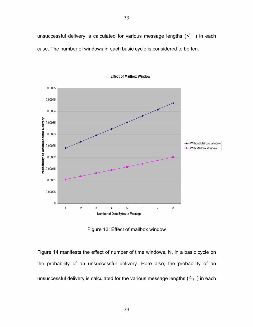
4.1.1 Results
Figure 13 compares the effect of two cases, one with the Mailbox Window and
the other one without the Mailbox Window. The value of the probability of an
32
33
unsuccessful delivery is calculated for various message lengths ( ) in each
case. The number of windows in each basic cycle is considered to be ten.
ic
Effect of Mailbox Window
0
0.00005
0.0001
0.00015
0.0002
0.00025
0.0003
0.00035
0.0004
0.00045
0.0005
1 2 3 4 5 6 7 8
Number of Data Bytes in Message
Pro
bab
ility
of
Un
succ
essf
ul D
eliv
ery
Without Mailbox WindowWith Mailbox Window
Figure 13: Effect of mailbox window
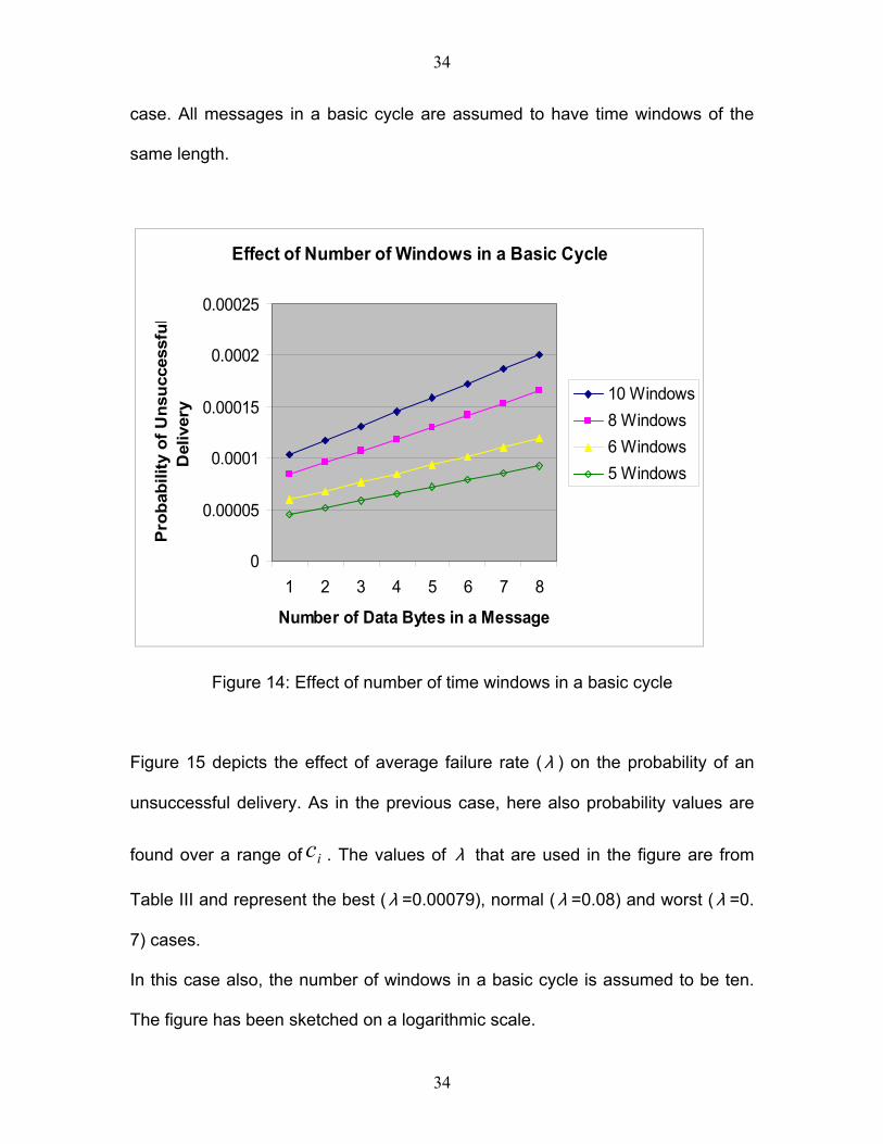
Figure 14 manifests the effect of number of time windows, N, in a basic cycle on
the probability of an unsuccessful delivery. Here also, the probability of an
unsuccessful delivery is calculated for the various message lengths ( ) in each ic
33
34
case. All messages in a basic cycle are assumed to have time windows of the
same length.
Effect of Number of Windows in a Basic Cycle
0
0.00005
0.0001
0.00015
0.0002
0.00025
1 2 3 4 5 6 7 8
Number of Data Bytes in a Message
Pro
babi
lity
of U
nsuc
cess
ful
Del
iver
y 10 Windows8 Windows6 Windows5 Windows
Figure 14: Effect of number of time windows in a basic cycle
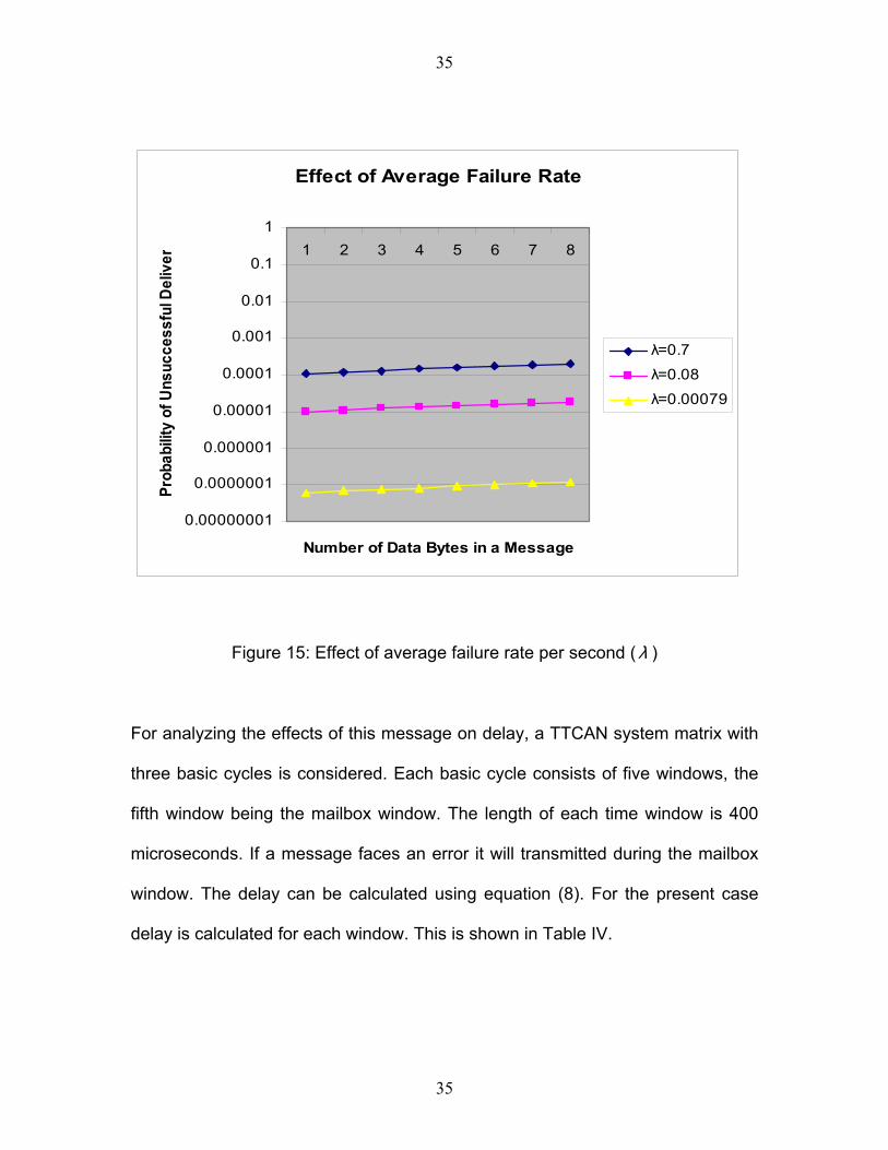
Figure 15 depicts the effect of average failure rate ( λ ) on the probability of an
unsuccessful delivery. As in the previous case, here also probability values are
found over a range of . The values of ic λ that are used in the figure are from
Table III and represent the best (λ =0.00079), normal ( λ =0.08) and worst (λ =0.
7) cases.
In this case also, the number of windows in a basic cycle is assumed to be ten.
The figure has been sketched on a logarithmic scale.
34
35
Effect of Average Failure Rate
0.00000001
0.0000001
0.000001
0.00001
0.0001
0.001
0.01
0.1
11 2 3 4 5 6 7 8
Number of Data Bytes in a Message
Prob
abilit
y of
Uns
ucce
ssfu
l Del
iver
λ=0.7
λ=0.08
λ=0.00079
Figure 15: Effect of average failure rate per second (λ )
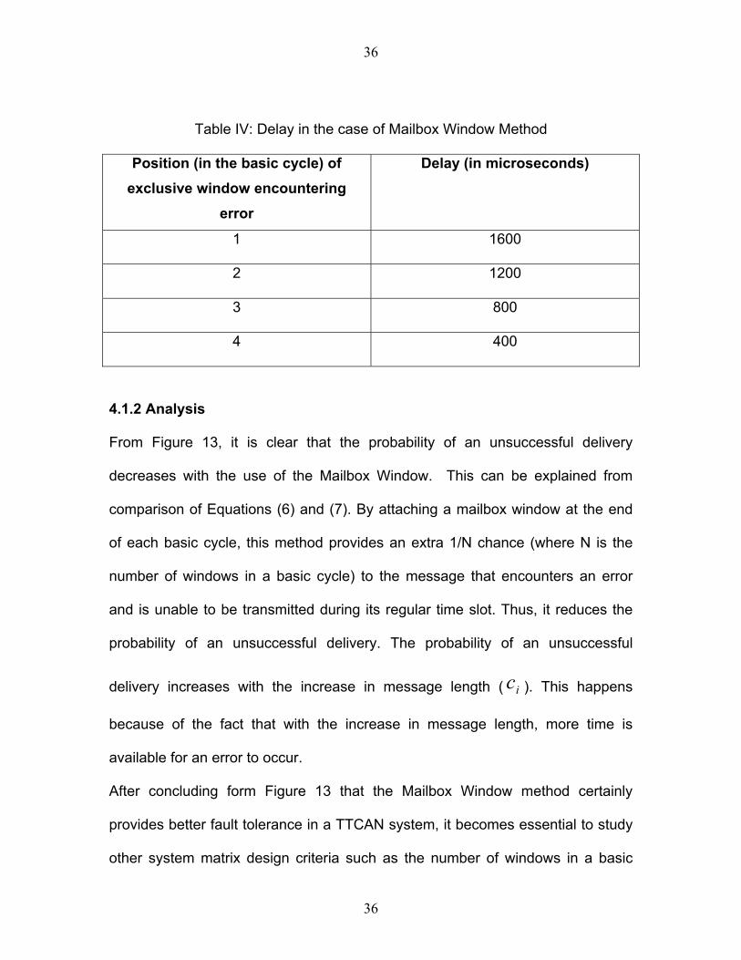
For analyzing the effects of this message on delay, a TTCAN system matrix with
three basic cycles is considered. Each basic cycle consists of five windows, the
fifth window being the mailbox window. The length of each time window is 400
microseconds. If a message faces an error it will transmitted during the mailbox
window. The delay can be calculated using equation (8). For the present case
delay is calculated for each window. This is shown in Table IV.
35
36
Table IV: Delay in the case of Mailbox Window Method
Position (in the basic cycle) of exclusive window encountering
error
Delay (in microseconds)
1 1600
2 1200
3 800
4 400
4.1.2 Analysis
From Figure 13, it is clear that the probability of an unsuccessful delivery
decreases with the use of the Mailbox Window. This can be explained from
comparison of Equations (6) and (7). By attaching a mailbox window at the end
of each basic cycle, this method provides an extra 1/N chance (where N is the
number of windows in a basic cycle) to the message that encounters an error
and is unable to be transmitted during its regular time slot. Thus, it reduces the
probability of an unsuccessful delivery. The probability of an unsuccessful
delivery increases with the increase in message length ( ). This happens
because of the fact that with the increase in message length, more time is
available for an error to occur.
ic
After concluding form Figure 13 that the Mailbox Window method certainly
provides better fault tolerance in a TTCAN system, it becomes essential to study
other system matrix design criteria such as the number of windows in a basic
36
37
cycle. Figure 14 provides an insight to this aspect. Figure 14 shows that the
probability of a failed delivery decreases with the decrease in number of windows
in a basic cycle. A mailbox window can be viewed as an extra chance of delivery
for failed messages. This chance of delivery is distributed over N windows. Thus
this chance is inversely proportional to N. If N is decreased, then the chance of
delivery is increased and vice versa. Hence, the probability of an unsuccessful
delivery will decrease as N decreases. This explains the nature of curves in
Figure 14. The figure helps in choosing the size of a basic cycle in a system
matrix for a given message size and an acceptable probability of an unsuccessful
delivery.
The effect of the best, worst and normal values of λ on the probability of a failed
message is shown in Figure 15. These values were collected during a study [16]
conducted in various conditions like laboratory conditions (best value ofλ ),
factory conditions (normal value ofλ ) and in a factory with arc welding taking
place at a two-meter distance (worst case value of λ ). Form the abovementioned
figure it is clear that in the worst-case scenario the probability of an unsuccessful
delivery increases.
The delay in the delivery of the message depends on the length of basic cycle
and position of the exclusive window in which the error occurred; this is evident
from Table IV. The earlier the error occurs in the basic cycle more it has to wait
for the mailbox time slot. The effect of the length of basic cycle can be shown
from the following consideration. In the case mentioned in section 4.1.1 there are
five windows in a basic cycle of length 400 microseconds each. If an error occurs
37
38
in the first exclusive window then message is received after 1600 microseconds
of deadline as shown in Table IV. However if there were ten windows in the basic
cycle everything else remaining same this message would have reached 3600
microseconds after its deadline. Thus it is better to have shorter basic cycles in
case of Mailbox Window method.
4.2 Performance Analysis of Arbitration Window Method
The chosen performance metrics for the Arbitration Window method are the
probability of an unsuccessful delivery of a message and delay in delivery of
message. The probability can be analyzed with the help of Equation (6) derived
in Section 3.2.3 and (10) derived in Section 3.3.3 of this work.
The performance of the proposed system has been analyzed by varying the
average rate of failure per second (λ ) and the worst-case length of a message
( ). The values for ic λ have been chosen as discussed in the case of the Mailbox
Window method. The bus speed is assumed to be 250 kbps
4.2.1 Results
Figure 16 shows two cases, one where the TTCAN is implemented according to
the Arbitration Window technique and the other where normal TTCAN is
implemented. The effect of the Arbitration Window method is noted on the
probability of an unsuccessful delivery. This effect is calculated for various
message lengths. The average rate of failure per second considered for the set
of results shown in Figure 16 is 0.7. The figure is drawn on a logarithmic scale.
38
39
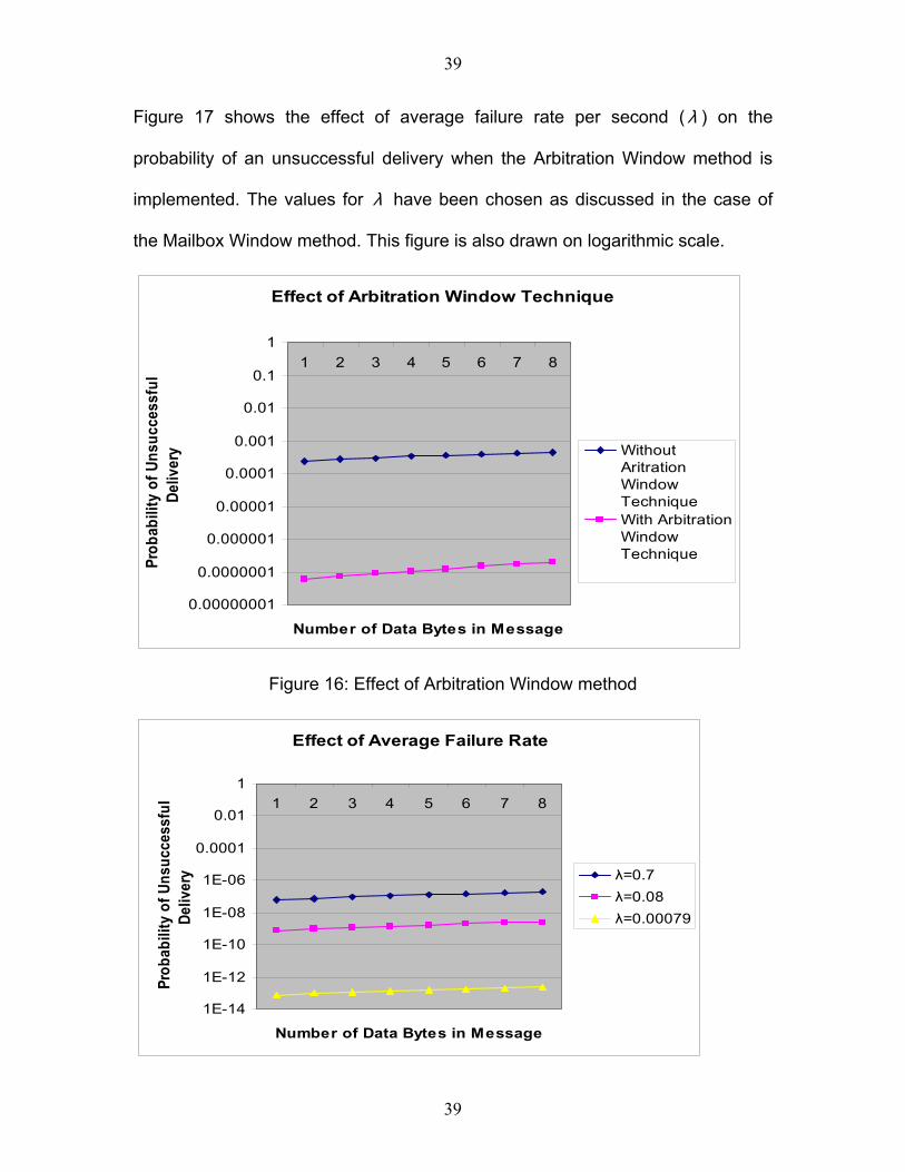
Figure 17 shows the effect of average failure rate per second ( λ ) on the
probability of an unsuccessful delivery when the Arbitration Window method is
implemented. The values for λ have been chosen as discussed in the case of
the Mailbox Window method. This figure is also drawn on logarithmic scale.
Effect of Arbitration Window Technique
0.00000001
0.0000001
0.000001
0.00001
0.0001
0.001
0.01
0.1
11 2 3 4 5 6 7 8
Number of Data Bytes in Message
Prob
abili
ty o
f Uns
ucce
ssfu
lDe
liver
y WithoutAritrationWindowTechniqueWith ArbitrationWindowTechnique
Figure 16: Effect of Arbitration Window method
Effect of Average Failure Rate
1E-14
1E-12
1E-10
1E-08
1E-06
0.0001
0.01
11 2 3 4 5 6 7 8
Number of Data Bytes in Message
Prob
abili
ty o
f Uns
ucce
ssfu
lDe
liver
y λ=0.7λ=0.08λ=0.00079
39
40
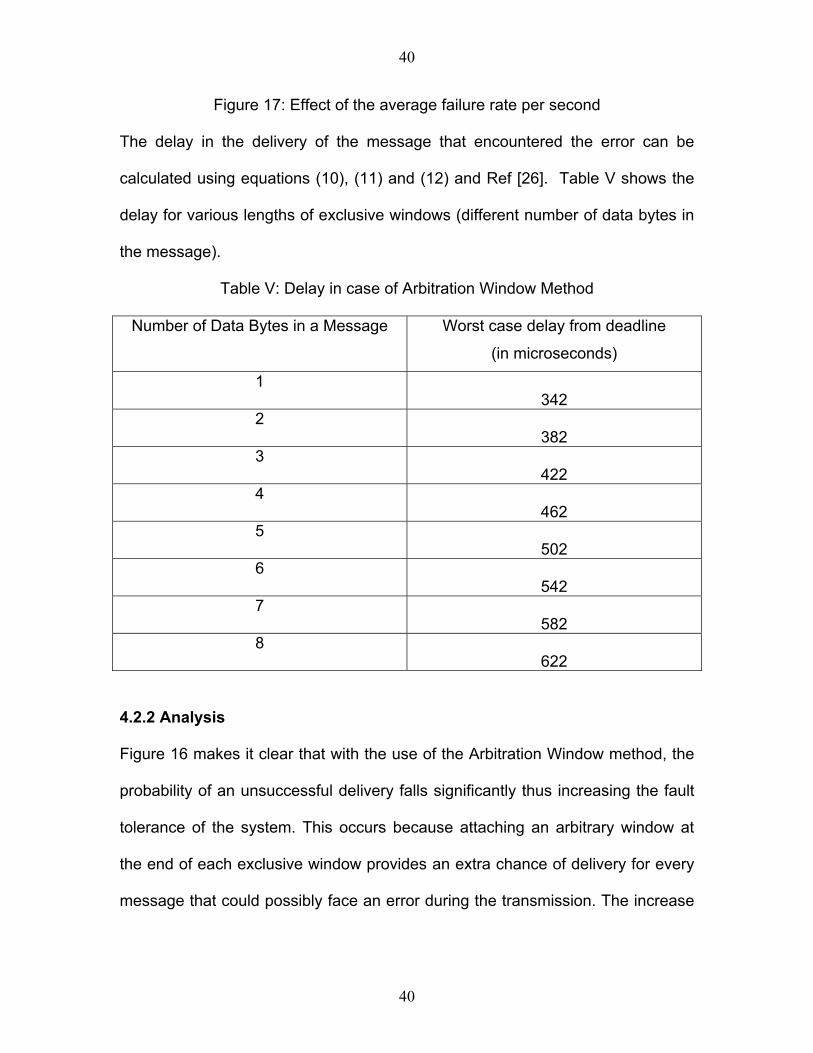
Figure 17: Effect of the average failure rate per second
The delay in the delivery of the message that encountered the error can be
calculated using equations (10), (11) and (12) and Ref [26]. Table V shows the
delay for various lengths of exclusive windows (different number of data bytes in
the message).
Table V: Delay in case of Arbitration Window Method
Number of Data Bytes in a Message Worst case delay from deadline
(in microseconds)
1 342
2 382
3 422
4 462
5 502
6 542
7 582
8 622
4.2.2 Analysis
Figure 16 makes it clear that with the use of the Arbitration Window method, the
probability of an unsuccessful delivery falls significantly thus increasing the fault
tolerance of the system. This occurs because attaching an arbitrary window at
the end of each exclusive window provides an extra chance of delivery for every
message that could possibly face an error during the transmission. The increase
40
41
of probability of an unsuccessful delivery with the increase in the message size
can be attributed to the extended exposure of the message to error occurrence.
Figure 17 shows the effect of the average rate of failure per second ( λ ) on the
probability of an unsuccessful delivery when the Arbitrary Window method is
used. As expected in the worst-case scenario, that is, when λ is equal to 0.7,
the probability of an unsuccessful delivery is more than what it is in the best-case
(λ equal to 0.0079). These values of λ were collected in conditions stated in
Section 4.1.3 (analysis of mailbox window method)
Table V shows the worst case delay for the message encountering error based
on the length of exclusive window for which it was scheduled. The delay is
directly proportional to the length of exclusive window facing error since this is
amount of time for which a message has to wait in order to be transmitted in the
next time slot which is an arbitrating window, as per proposed system matrix. As
can be seen from the Table V maximum possible delay is 622 microseconds.
Unlike mailbox window method, delay in this case is independent of length of
basic cycle.
4.3 Performance Analysis of the Asynchronous Redundant Bus Method
The Asynchronous Redundant Bus method has been analyzed by software
simulation. The purpose of the simulation is to collect results that can help in
finding the average latency when the redundant bus is used. The simulation
setup is described as follows. There are two buses and five nodes. The primary
bus is the one on which all the time triggered communications are carried out and
41
42
the dedicated redundant secondary bus is the one which handles
communications in case of a transmission failure on the primary bus. The speed
of the primary bus is 250 kbps. The speed of the secondary bus is varied as a
percentage of the primary bus speed. The system matrix consists of three basic
cycles. Each basis cycle contains five exclusive time windows of 400
microseconds each. Bus loading is 75 percent. The average failure rate per
second ( λ ) is chosen as 0.7 (the worst-case scenario). The percentage error
according to the chosen value of λ and configuration of the system matrix is
0.00029. The time window in which an error occurs and the point of occurrence
of the error within that time window, both are chosen randomly. As mentioned
earlier, it is being assumed that for any practical fault tolerant system, occasional
delivery failures are acceptable and expected and that the hard deadline cannot
be met in any form of electrical communications that are subject to unpredictable
faults [23]. In this work, the acceptable delay past the deadline is taken as 1200
microseconds. Any message with a delay exceeding this limit should be rejected.
4.3.1 Results
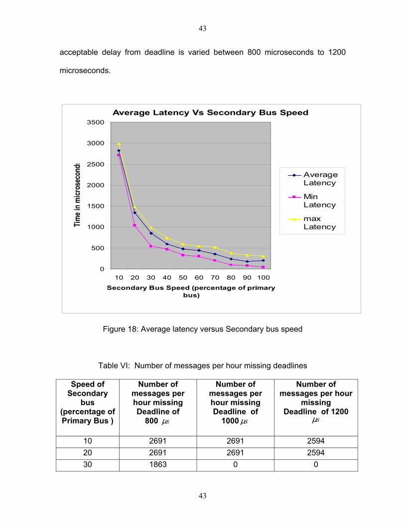
Figure 18 shows the variation of the maximum, minimum and average latencies
of messages that faced failure during transmission through the primary bus. This
variation is shown for various secondary bus speeds. The secondary bus speed
is shown as a percentage of the primary bus speed, which is 250 kbps.
Table IV shows the number of messages per hour (taking the secondary bus)
that exceed the maximum delay beyond the deadline. The value of this
42
43
acceptable delay from deadline is varied between 800 microseconds to 1200
microseconds.
Average Latency Vs Secondary Bus Speed
0
500
1000
1500
2000
2500
3000
3500
10 20 30 40 50 60 70 80 90 100
Secondary Bus Speed (percentage of primary bus)
Time i
n micr
osec
onds
AverageLatency
MinLatency
maxLatency
Figure 18: Average latency versus Secondary bus speed
Table VI: Number of messages per hour missing deadlines
Speed of Secondary
bus (percentage of Primary Bus )
Number of messages per hour missing Deadline of
800 sµ
Number of messages per hour missing Deadline of
1000 sµ
Number of messages per hour
missing Deadline of 1200
sµ
10 2691 2691 2594 20 2691 2691 2594 30 1863 0 0
43
44
40 0 0 0 50 0 0 0
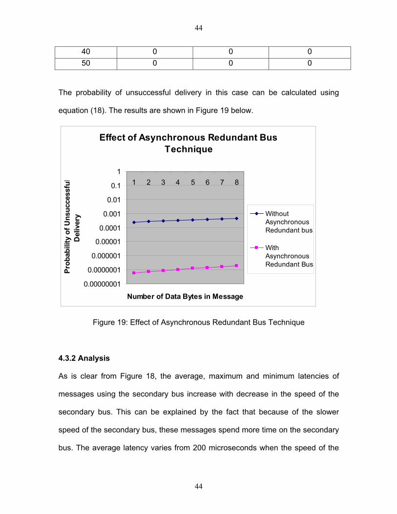
The probability of unsuccessful delivery in this case can be calculated using
equation (18). The results are shown in Figure 19 below.
Effect of Asynchronous Redundant Bus Technique
0.00000001
0.0000001
0.000001
0.00001
0.0001
0.001
0.01
0.1
11 2 3 4 5 6 7 8
Number of Data Bytes in Message
Prob
abili
ty o
f Uns
ucce
ssfu
lD
eliv
ery Without
AsynchronousRedundant bus
WithAsynchronousRedundant Bus
Figure 19: Effect of Asynchronous Redundant Bus Technique
4.3.2 Analysis
As is clear from Figure 18, the average, maximum and minimum latencies of
messages using the secondary bus increase with decrease in the speed of the
secondary bus. This can be explained by the fact that because of the slower
speed of the secondary bus, these messages spend more time on the secondary
bus. The average latency varies from 200 microseconds when the speed of the
44
45
secondary bus is the same as that of the primary bus to 2828 microseconds
when the speed of the secondary bus is ten percent of the speed of primary bus.
It becomes essential to determine the speed of the secondary bus for a good
fault tolerant TTCAN system design. In order to determine the speed of the
secondary bus to be used, it is necessary to consider the acceptable delay after
the deadline of the message. Table IV shows the number of messages per hour
that miss the extended deadline. Three cases have been studied where the
extension of the deadline is considered as 800 microseconds, 1000
microseconds and 1200 microseconds. From Table IV it becomes clear that
when the secondary bus speed is approximately equal to 30 to 40 percent of the
primary bus speed almost all messages are able to make it to the receivers
within 1200 microseconds of deadline. Consider a car moving at 50kmph.
Suppose on the application of the brake, the ABS message encounters a
transmission error. This message is then sent through the secondary bus with
the bus speed equal to 40 percent of the primary bus speed. This message will
definitely reach the intended receiver within 1200 microseconds. In these 1200
microseconds, the car will move only 1.6 centimeters. This distance is
insignificant, especially when compared to the case when there is no secondary
bus and this message is completely lost leading to break failure or delayed by
one period. Thus it can be concluded that it is practical to use an asynchronous
redundant bus for introducing fault tolerance in a TTCAN system.
From Figure 19 it is clear that the probability of unsuccessful failure decreases
with use of asynchronous redundant bus. The results shown in Figure 19 and the
45
46
results shown in Figure 16 for effect of Arbitration Window Method are identical
since both methods are effectively providing the message facing an error two
attempts for delivery.
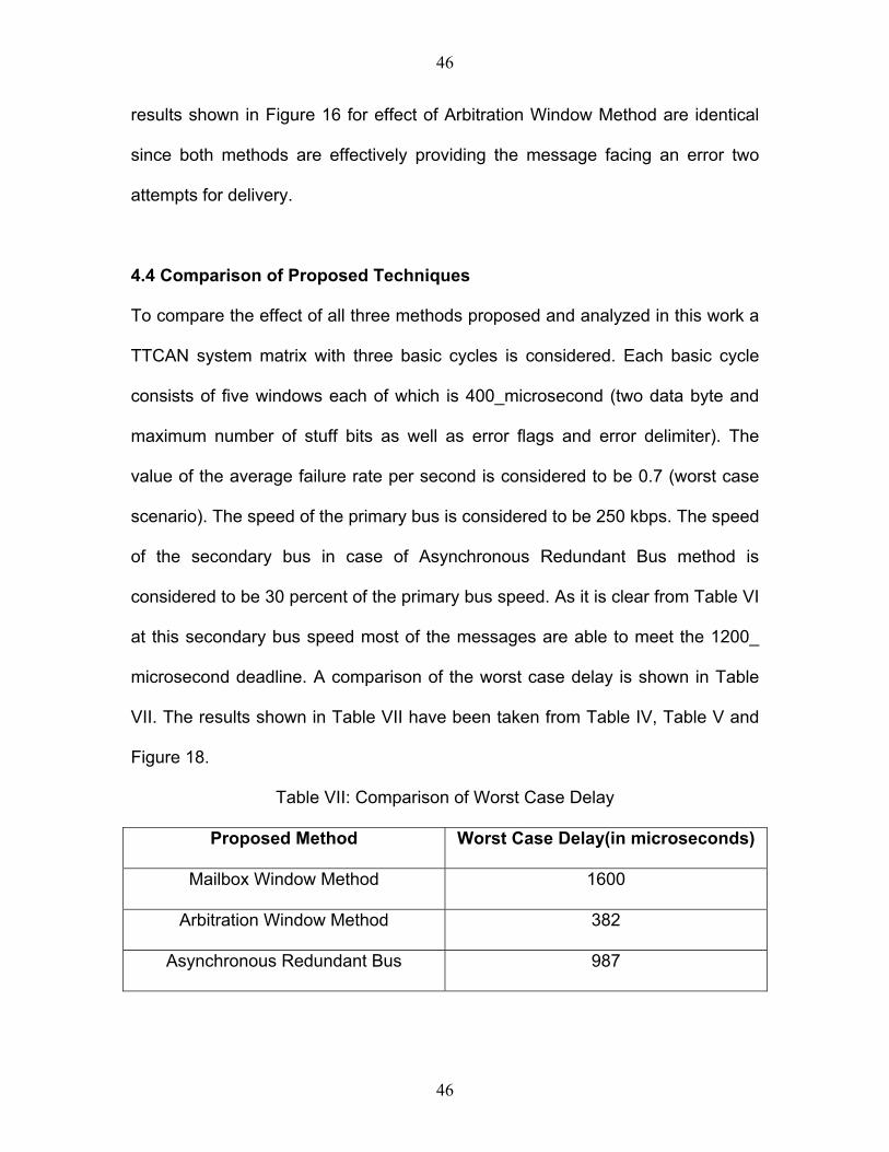
4.4 Comparison of Proposed Techniques
To compare the effect of all three methods proposed and analyzed in this work a
TTCAN system matrix with three basic cycles is considered. Each basic cycle
consists of five windows each of which is 400_microsecond (two data byte and
maximum number of stuff bits as well as error flags and error delimiter). The
value of the average failure rate per second is considered to be 0.7 (worst case
scenario). The speed of the primary bus is considered to be 250 kbps. The speed
of the secondary bus in case of Asynchronous Redundant Bus method is
considered to be 30 percent of the primary bus speed. As it is clear from Table VI
at this secondary bus speed most of the messages are able to meet the 1200_
microsecond deadline. A comparison of the worst case delay is shown in Table
VII. The results shown in Table VII have been taken from Table IV, Table V and
Figure 18.
Table VII: Comparison of Worst Case Delay
Proposed Method Worst Case Delay(in microseconds)
Mailbox Window Method 1600
Arbitration Window Method 382
Asynchronous Redundant Bus 987
46
47
Thus we see that for the given system configuration the Arbitration Window
method has the least delay which is equal to 382 microseconds. Even when a
message with eight data bytes is used this delay does not exceed 622
microseconds, which is still lesser than the delay in the other two cases.
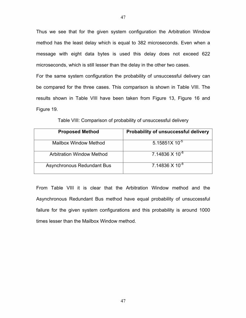
For the same system configuration the probability of unsuccessful delivery can
be compared for the three cases. This comparison is shown in Table VIII. The
results shown in Table VIII have been taken from Figure 13, Figure 16 and
Figure 19.
Table VIII: Comparison of probability of unsuccessful delivery
Proposed Method Probability of unsuccessful delivery
Mailbox Window Method 5.15851X 10⁻⁵
Arbitration Window Method 7.14836 X 10⁻⁸
Asynchronous Redundant Bus 7.14836 X 10⁻⁸
From Table VIII it is clear that the Arbitration Window method and the
Asynchronous Redundant Bus method have equal probability of unsuccessful
failure for the given system configurations and this probability is around 1000
times lesser than the Mailbox Window method.
47
48
5 CONCLUSION
The work presented in this thesis is an effort to increase fault tolerance of
TTCAN systems. In case of an error, retransmission of a message is not allowed
in an exclusive window of TTCAN. This can cause loss of safety critical
messages, thus putting life of passengers at risk. The thesis work presented here
proposes three solutions to address this issue. The work provides a detailed
description of architectures and algorithms required to implement these
schemes. The parameters considered for measuring the effects of these
schemes on the fault tolerance of the system are probability of unsuccessful
delivery and the delay in the delivery of the message. The results of a given
system configuration are compared at the end of work. The first method known
as the Mailbox Window Method is useful only when the length of the basic cycle
is small, messages have short periods and no hardware solution is available. The
second method called the Arbitration Window Method has the least delay in all
cases and requires no hardware changes. It has the lower probability of
unsuccessful delivery than the Mailbox Window Method but equal to the
probability of unsuccessful delivery in case of third method (known as the
Asynchronous Redundant Bus Method). Also, here the delay is not dependent on
the length of a basic cycle. The only drawback of this method is that it requires
periods of messages to be long enough to incorporate an arbitration window
following every exclusive window. The third method is known as Asynchronous
Redundant bus method requires hardware changes in the system as it requires a
secondary bus. This method is suitable for the cases where multiple number of
48
49
low speed busses exist that are used for carrying out communication of non
safety critical methods. For this method the probability of unsuccessful delivery is
equal to that of the Arbitration Window method but lesser that the Mailbox
Window method. The delay in delivery of messages can be reduced significantly
by using a high speed dedicated secondary bus. All three proposed methods
show improvement in fault tolerance of TTCAN system and are cost effective
when compared to existing techniques.
49
50
6 FUTURE WORK
The increase of drive-by-wire systems in the vehicles will give rise to extensive
use of real time in-vehicle networks. FlexRay is a communication system that will
support the needs of future in-car control applications. FlexRay will provide
flexibility and determinism by combining a scalable static and dynamic message
transmission, incorporating the advantages of familiar synchronous and
asynchronous protocols.
FlexRay Consortium (Core members consist of BMW, DaimlerChrysler, Motorola,
Philips, GM and Bosch) have been working together in developing the
requirements for an advanced communication system for future automotive
applications. These six companies have brought together their respective areas
of expertise to define a communication system that is targeted to support the
needs of future in-car control applications.
However, FlexRay is still in specification development phase. It will take four to
five years to implement it completely and to start manufacturing components
supporting FlexRay commercially. Till then, Time Triggered CAN can be used as
protocol for supporting real time applications. It is essential to ensure fault
tolerance in TTCAN. The work presented in this thesis can be used introduce
fault tolerance in TTCAN.
Any real time safety critical application of CAN in the field of Industrial
Automation can also utilize these schemes for increasing fault tolerance.
50
51
REFERENCES
1. Karen Parnell, “Automotive Electronics Digital Convergence-How to Cope
with Emerging Standards and Protocols”, AMAA 2004, Berlin.
2. Stephen Channon and Peter Miller,” The Requirements of Future In-
Vehicle Networks and an Example Implementation”, SAE Technical Paper
Series 2004-01-0206.
3. Rienhard Maier, et al,” Time Triggered Architecture: A Consistent
Computing Platform “, IEEEmicro July/Aug 2002.
4. Patrick Leteinturier, et al,” TTCAN from applications to products in
automotive”, SAE Technical Paper Series 2003-01-0114.
5. Maria Bruce,” Distributed Brake–By-Wire Based on TTP/C”, ISSN 0280-
5316 ISRN LUTFD2/TFRT-5668 SE.
6. http://sciencedaily.com/releases/1998/119811031415.htm
7. S Shaheen, D Heffernan and G Leen,” A Comparison of Emerging Time
Triggered Protocols for X-by-wire Control Networks”, Proc. Instn Mech.
Engrs Vol 217 PartD: J.Automobile Engineering.
8. Christopher A. Lupini,”Multiplex Bus Progression 2003”, SAE Technical
Paper Series 2003-01-0111.
9. G Leen and D Heffernan,” Expanding Automotive Electronic Systems”,
IEEE Computer Jan 2002 P.88.
10. Naill Murphy,” A Short trip on the CAN bus”, Embedded System
Programming (8/11/03), embedded.com.
51
52
11. M.Farsi, et al,” An overview of CAN”, Computing and Control Engineering
Journal, June 1999.
12. Florian Hartwich, et al,” Integration of Time Triggered CAN (TTCAN_TC)”,
SAE Technical Paper Series, 2002-01.
13. http://www.can.bosch.com/content/TTCAN.html
14. www.tttech.com/technology/docs/protocol_comparisons/TTTech-
comparison_TTP-TTCAN-FlexRay.pdf
15. Thomas Fuehrer, et al,” Time Triggered Can (TTCAN)”, SAE Technical
Paper Series 2001-01-0073.
16. Joaquin Ferreira , Arnaldo Oliveria ,et al,” An Experiment to Assess Bit
Error Rate in CAN”, RTN 2004 - 3rd Int. Workshop on Real-Time Networks,
Catania, Italy.
17. Cedric Wilwert, et al, “Impact of Fault Tolerance Mechanisms on X-by-wire
System Dependability “,TRIO report 2003.
18. Guillermo Rodriguez-Navas, et al, “Harmonizing Dependability and Real
Time in CAN Networks”, RTLIA2003 - 2nd International Workshop on
Real-Time LANs in the Internet Age.
19. http://www.tttech.com/technology/docs/fault_handling/TTTech-Fault-
Handling-TTA.pdf
20. Holger Zeltwanger,”Time-Triggered communication on CAN”, SAE
Technical Paper Series 2002-01-0437.
21. B.Mϋller, et al,”Fault Tolerant TTCAN networks”, 8th iCC Las Vegas,
2002.
52
53
22. Matjaz Colnaric, Domen Verber,” Communication Infrastructure for IFATIS
Distributed Embedded Control Application”, RTN 2004 - 3rd Int. Workshop
on Real-Time Networks, Catania, Italy.
23. Ian Boster, Alan Burns, et al,”Comparing Real-Time Communication under
Electromagnetic Interference”, 16th Euromicro Conference on Real-Time
Systems (ECRTS'04), 2004 Catania, Italy
24. http://www.engin.umd.umich.edu/ceep/reports/200MidYearRichardson01.
html
25. Jose Rufino, “An Overview of Controller Area Network”, Proceedings of
CiA Forum- CAN for Newcomers, January 1997, Braga, Portugal.
26. http://www.esacademy.com/faq/calc/can.htm
53

54
ABSTRACT
DESIGN AND PERFORMANCE ANALYSIS OF FAULT TOLERANT TTCAN SYSTEM
by
AAKASH ARORA
MAY 2005
Advisor: Dr. Syed Masud Mahmud
Major: Computer Engineering
Degree: Master of Science
Continuous demand for fuel efficiency mandate “Drive-by-Wire” systems. The
goal of Drive-by-wire is to replace nearly every automotive hydraulic/mechanical
system with electronics. Drive-by-Wire and active collision avoidance systems
need fault tolerant networks with time triggered protocols, to guarantee
deterministic latencies. CAN is an event triggered protocol which has features
like high bandwidth, error detection, fault confinement and collision avoidance
based on message priority. However, CAN do not ensure message latency,
which is critical for real time application. TTCAN (Time Triggered CAN) removes
this fallacy of CAN by providing exclusive time windows for those messages that
need deterministic latencies. In addition to the exclusive windows, there are
arbitration windows too, which make way for event triggered communications. In
TTCAN, if an error occurs within an exclusive or arbitration window,
retransmission of the message is not allowed. If the message that encountered
54
55
the error is a safety critical message, then the transmission error can
compromise the safety of the vehicles. The thesis work presented here proposes
three techniques to increase fault tolerance of TTCAN systems. The proposed
techniques increase fault tolerance of TTCAN systems by improving system
matrix design and incorporating redundant bus. A detailed description of
architectures and algorithms required to implement these techniques has been
presented. These techniques have been studied analytically and by using
simulation. The results show significant improvement in the fault tolerance of
TTCAN.
55
56
AUTOBIOGRAPHICAL STATEMENT
AAKASH ARORA
I received my Bachelors degree in Mechanical Engineering from Punjab Engineering College, Chandigarh, India. My pursuit for challenging career in the field of automobiles helped me in making the decision to come to Detroit and to pursue higher degree in the field of Computer Engineering. I was lucky to be member of Dr. Syed M Mahmud’s IVTS research group at Wayne State University. Under able guidance of Dr. Mahmud, I was able to acquire knowledge and skills in the field of CAN and TTCAN. I have published papers mainly in the area of fault tolerant in-vehicle networks. I have designed and analyzed various methods to introduce fault tolerance in TTCAN. The details of algorithms, architectures and analysis of these methods are the major contribution of my thesis work. I have done internships at Suzuki India Limited and at Siemens Energy and Automation, Automotive Business Unit, Troy, Michigan. I have been selected for Engineering Rotation Program at Motorola Automotive, Deer Park, Illinois. In future also, I hope to contribute to the automotive world to the best my capabilities. My leisure time activities include playing basketball, running, listening to music, reading inspirational books, visiting new places and watching movies.
Publications: 1. Aakash Arora and Syed Masud Mahmud “Performance Analysis of a
Fault Tolerant TTCAN System ”, Proc. of the SAE 2005 World Congress, April 11-14, 2005, Detroit, Michigan, USA, Paper Number 2005-01-1538.
2. Aakash Arora, Praveen Ramteke and Syed Masud Mahmud, “A Fault Tolerant Time Triggered Protocol for Drive-by-Wire Systems,” proceedings
of the 4th
Annual Intelligent Vehicle Systems Symposium of National Defense Industries Association (NDIA), National Automotive Center and Vectronics Technology, June 22 –24, 2004, Traverse City, Michigan.
3. Praveen Ramteke, Aakash Arora and Syed Masud Mahmud “Feasibility of using Vehicle’s Power Line as a Communication Bus”, Proceedings
of the 4th
Annual Intelligent Vehicle Systems Symposium of National Defense Industries Association (NDIA), National Automotive Center and Vectronics Technology, June 22 –24, 2004, Traverse City, Michigan.
56
Recommended