Demand Reduction and Inefficiency in Multi-Unit AuctionsLawrence M. Ausubel and Peter Cramton*
University of Maryland
20 March 1998
(first draft: 8 November 1995)
Abstract
Auctions typically involve the sale of many related goods. The FCC spectrum auctions
and the Treasury debt auctions are examples. With conventional auction designs, large
bidders have an incentive to reduce demand in order to pay less for their winnings. This
incentive creates an inefficiency in multi-unit auctions. Large bidders reduce demand for
additional units and so sometimes lose to smaller bidders with lower values. We
demonstrate this inefficiency in several auction settings: flat demand and downward-
sloping demand, independent private values and correlated values, and uniform pricing
and pay-your-bid pricing. We also establish that the ranking of the uniform-price and
pay-your-bid auctions is ambiguous. We show how a Vickrey auction avoids this
inefficiency and how the Vickrey auction can be implemented with a simultaneous,
ascending-bid design (Ausubel 1997). Bidding behavior in the FCC spectrum auctions
illustrates the incentives for demand reduction and the associated inefficiency.
JEL No.: D44 (Auctions)Keywords: Auctions, Multi-Unit Auctions, Spectrum Auctions, Treasury Auctions
Send comments to:
Professors Lawrence M. Ausubel or Peter CramtonDepartment of EconomicsUniversity of MarylandCollege Park, MD 20742-7211
[email protected] [email protected](301) 405-3495 (301) 405-6987
*The authors gratefully acknowledge the support of the National Science Foundation. We appreciatevaluable comments from Preston McAfee, three anonymous referees, and participants at numerousconferences and seminars.
2
Demand Reduction and Inefficiency in Multi-Unit AuctionsLawrence M. Ausubel and Peter Cramton
1 IntroductionOne of the preeminent justifications for auctioning public resources is to attain allocative efficiency.
For example, the bidder information package for the much-heralded Broadband PCS Auction began with
a letter by Reed E. Hundt, Chairman of the Federal Communications Commission, who wrote, “I am
confident that the auction method we have chosen for selecting licensees will put the spectrum in the
hands of those who most highly value it and who have the best ideas for its use.” Similarly, in opening
remarks for the December 5, 1994 auction, Vice President Al Gore said, “Now we're using the auctions to
put licenses in the hands of those who value them the most.”
Given the emphasis that policymakers have placed on efficiency, surprisingly little is known by
economists about the efficiency properties of various auction designs for multiple items. Within the realm
of auctioning a single, indivisible item, it is understood that the second-price sealed-bid auction and the
English auction induce buyers to bid sincerely, implying efficient outcomes (William Vickrey 1961).
Under a first-price sealed-bid auction, buyers shade their bids relative to their values, but efficiency is still
possible when there are symmetric bidders (who employ symmetric strategies). Settings with multiple
identical items, where each bidder has taste for only one item, yield similar results.
However, in environments with multiple units and bidders who each may desire multiple units,
general results about even the most common auction forms remain elusive. This observation is clearest
within the context of setting the rules for the U.S. Treasury auction, where there has been a heated and
longstanding debate between two alternatives. The traditional format used for the sale of Treasury
securities has been the pay-your-bid auction (also known as the “discriminatory auction”): bidders each
submit bids for various quantities at various prices and the auctioneer determines the market-clearing
price; all bids exceeding the market-clearing price are accepted. Milton Friedman (1960) proposed the
uniform-price auction (also known as the “nondiscriminatory auction” or “competitive auction”): bidders
again each submit bids for various quantities at various prices and the auctioneer determines the market-
clearing price; bidders again are awarded the quantities which they demanded at the market-clearing price
but now are charged only the market-clearing price (as opposed to the actual prices they bid) for each unit
they win.
Most public debate about the relative merits of these two sets of rules has been misled by an
imperfect analogy between single-unit and multi-unit auctions. Academics and policymakers, alike, have
observed that the pay-your-bid auction can be viewed as a multi-unit extension of the first-price auction,
3
and have asserted that the uniform-price auction is best regarded as a multi-unit extension of the second-
price auction. This flawed analogy has led to a variety of assertions and speculations. At the extreme, this
has led otherwise-astute economists to incorrectly posit that the uniform-price auction inherits the same
attractive truth-telling attributes as the second-price sealed-bid auction, and hence yields efficient
outcomes. It has also led observers to wrongly infer that the uniform-price auction ought to — as a
general theoretical matter — generate greater expected seller revenues than a pay-you-bid auction.
In the second-price auction of a single item (with independent private values), bidding one's own true
value is a weakly-dominant strategy. The notion that sincere bidding does not extend to a uniform-price
auction where bidders desire multiple units originates in the seminal work of Vickrey (1961).
Nevertheless, what might be called the “uniform-price auction fallacy” is still often made in the 1990s,
most conspicuously in discussions on reforming the U.S. Treasury auction in the aftermath of the 1991
Salomon Brothers scandal. In the Wall Street Journal (August 28, 1991), Friedman appears to assert that
with a uniform-price auction one simply bids one's reservation value: “A [uniform-price] auction
proceeds precisely as [a pay-your-bid auction] with one crucial exception: All successful bidders pay the
same price, the cut-off price. An apparently minor change, yet it has the major consequence that no one is
deterred from bidding by fear of being stuck with an excessively high price. You do not have to be a
specialist. You need only know the maximum amount you are willing to pay for different quantities.”
Merton Miller, in an interview with the New York Times (September 15, 1991, 3:13), emphasizes bid-
shading as the main disadvantage of the pay-your-bid auction used by the Treasury: “People will shave
their bids down. … All of that is eliminated if you use the [uniform-price] auction. You just bid what you
think it's worth.” The Joint Report on the Government Securities Market (1992, p. B-21), jointly signed
by the Treasury Department, the Securities and Exchange Commission, and the Federal Reserve Board,
states: “Moving to a uniform-price award method permits bidding at the auction to reflect the true nature
of investor preferences … . In the case envisioned by Friedman, uniform-price awards would make the
auction demand curve identical to the secondary market demand curve.”
One of the primary objectives of our current paper is to clear the air of the uniform-price auction
fallacy. We demonstrate, under general circumstances, that a bidder who desires more than one unit in a
uniform-price auction has an incentive to shade her bid. Moreover, we show that this demand reduction is
consequential to a policymaker concerned with putting items “in the hands of those who value them the
most.” We prove an Inefficiency Theorem which establishes that every equilibrium of the uniform-price
auction is ex post inefficient with positive probability.
A second objective of our paper is to specifically address the ranking of the pay-your-bid and
uniform-price auction. For almost 40 years, it has been an open question — both theoretically and
4
empirically — whether the pay-your-bid format or the uniform-price format would produce greater
revenue in the Treasury auction. Friedman (1960) conjectured that the uniform-price auction would
dominate the pay-your-bid auction, in revenue terms. This has led the U.S. Treasury to experiment with
the uniform-price rule in actual auctions of securities, with inconclusive results (see, for example,
Malvey, Archibald and Flynn 1996 and Reinhart and Belzer 1996). The question has also spawned an
extensive literature of laboratory experiments, which has tended to slightly favor the uniform-price
auction, except when bidders' demand curves are sufficiently steep (see, for example, Smith 1967, 1982).
Theoretical arguments have tended to draw the imperfect analogy from the single-item case. For example,
Chari and Weber (1992, p. 8) note that when each bidder demands only a single unit: “The uniform-price
(second-price) auction dominates the discriminatory (first-price) auction.” They then argue that the same
should hold for the general case: “Matters are more complicated when bidders have demand schedules
expressing the number of units they are willing to buy at various prices. While the theory has not been
completely developed for that situation, the economic logic of the arguments for the single-item
environment seem likely to carry over.”
In our paper, we compare the two auction formats over a class of models. Considering the twin
objectives of allocative efficiency and revenue maximization, we find that the ranking is inherently
ambiguous. We are able to construct reasonable specifications of demand where the pay-your-bid auction
dominates the uniform-price auction both on expected gains from trade and expected seller revenues. We
are also able to construct equally-reasonable specifications of demand where the reverse ranking holds.
Thus, if the seller is constrained to select between the pay-your-bid and uniform-price auction, the choice
ought to be viewed as an empirical question that depends on the actual nature of demands.
A third theme of our paper is that, if previous misunderstanding of multi-unit auctions has been
based on the flawed analogy involving the uniform-price auction, then future progress may result from
attention to a more perfect analogy. The correct extension of the second-price auction to contexts where
bidders have taste for more than one unit is Vickrey's multi-unit, sealed-bid auction: a bidder's payment
for the kth unit she wins equals the kth highest rejected bid entered by another bidder. The Vickrey auction
inherits the property of the second-price auction that sincere bidding is weakly dominant, so that you truly
“just bid what you think it's worth.” Consequently, the Vickrey auction yields allocatively-efficient
outcomes, truly putting items “in the hands of those who value them the most.” And, for a limited family
of models, we obtain the mechanism-design result that the Vickrey auction with a reserve price
maximizes the seller's revenues. It is therefore not unusual for the Vickrey auction to revenue-dominate
the uniform-price and pay-your-bid auctions, but the ranking depends on the empirical nature of demands.
5
Thus, if the U.S. Treasury (or any seller of multiple identical items) is free to choose among all
sealed-bid auction formats, it ought to consider adopting Vickrey's, rather than Friedman's, auction. A
seller of multiple identical items might also consider the alternative ascending-bid auction recently
proposed by Ausubel (1997), which is a dynamic auction whose static representation is the Vickrey
auction.
The theorems of our paper are formally stated with reference to static auctions of multiple identical
items, where bidders submit demand curves, and so the theorems are most obviously applicable to sealed-
bid auctions such as those for Treasury bills. However, most of our results can be immediately adapted to
any auction context where equilibria possess a uniform-price character. For example, suppose that
multiple identical items are sold simultaneously by auction, as in the simultaneous multiple round auction
used by the Federal Communications Commission to assign spectrum licenses, the ascending-bid auction
proposed in the Joint Report on the Government Securities Market (1992, pp. B-23–B-24), or the
venerable “silent auction” commonly used for charitable fund-raising. In each of these auction formats,
there is a strong tendency toward arbitrage of the prices for identical items. Indeed, in the FCC's
Nationwide Narrowband Auction of July 1994, similar licenses were on average priced within 0.3 percent
of the mean price for that category of license, and the five most desirable licenses sold (to three different
bidders) identically for $80,000,000 apiece. A useful way to conceptualize any of these auctions is to
think of each bidder as selecting the quantity of items she would like to purchase at every possible price
and then submitting the entire resultant demand curve to the auctioneer at the very start of the auction.
(This is an extension of the usual transformation which maps from the English auction to the sealed-bid,
second-price auction.) In the induced static auction, the corresponding payment rule is that of the highest
losing bid, so our results on uniform-price auctions are directly applicable.
Similarly, suppose that multiple identical items are sold through a sequence of English auctions.
While Ashenfelter (1989) has identified a declining-price anomaly — later lots of identical wines are
twice as likely to sell for lower prices than for higher prices, and the price of a second identical lot equals
on average only 96 to 99 percent the price of the first lot — prices are still relatively close to constant
over time. To the extent that prices in sequential auctions are intertemporally arbitraged, the outcome
maps to a uniform-price auction, and our Inefficiency Theorem still applies.
Finally, consider a situation where a seller simultaneously auctions multiple items, which while not
identical are still reasonable substitutes. (For example, consider the Federal Communications
Commission's auctions of PCS licenses.) Essentially all that is required for bid-shading is the presence of
strategic bidders who desire more than one item. Consequently, we would expect that the phenomena of
demand reduction and inefficiency to extend to the richer environment. This can be argued rigorously for
6
a sequence of auctions with nonidentical items, which converges to an auction of identical items.
Typically, the equilibrium correspondence is upper hemicontinuous, so that the limits of equilibria of the
auctions along the sequence should converge to an equilibrium of the limit of the auctions. Suppose that
each of the auctions with nonidentical items exhibited an ex post efficient equilibrium. Then the limit of
these equilibria would be an ex post efficient equilibrium of the auction with identical items, contradicting
our Inefficiency Theorem. Thus, we conclude that sufficiently far along the sequence, the auctions with
nonidentical items must also display only inefficient equilibria.
The intuition for bid shading and demand reduction in the uniform-price auction is as follows. When
a bidder desires multiple units of the good being auctioned, there is a positive probability that her bid on a
second or later unit will be pivotal, thus determining the price that the bidder pays on other units that she
wins. Given this, she has an incentive to bid less than her true value on later units in order to reduce the
price she will pay on the earlier units. With discrete goods, this intuition suggests that the bidder will bid
her true value on her first unit demanded, but strictly less than her true value on all subsequent units. With
continuously-divisible goods, this intuition suggests that a bidder's submitted demand curve will take on
the qualitative features of a monopolist's marginal-revenue curve: the vertical intercepts of the two curves
coincide, but at all positive quantities, the bid curve lies strictly below the true valuation curve.
The Inefficiency Theorem relies not only on bid shading but on differential bid shading. This point is
apparent from the standard first-price auction of a single item: every bidder shades her bid, but with
symmetric bidders and the symmetric equilibrium, there is nevertheless a monotonic function from values
to bids. Thus, by assigning the item to the highest bidder, the auction also puts the item in the hands
which value the item the most. What is needed to establish inefficiency is the presence of differential bid
shading: bidders with identical marginal valuations shading their bids by different amounts. Differential
shading is present in the uniform-price auction. With discrete goods, there is no bid shading on the first
unit demanded, but increasing amounts of bid shading on subsequent units. With continuously-divisible
goods, the bid curve diverges from the true valuation curve as the quantity increases. The intuition is
simply that the consequences of a bid being pivotal become increasingly great, the more units that the
bidder will wins.
The intuition for why the efficiency of the pay-your-bid auction may exceed that of the uniform-
price auction derives from the fact that the pay-your-bid auction is not subject to bid shading that is
increasing in quantity. Unlike a uniform-price auction, a bid for an additional unit in a pay-your-bid
auction has no effect on the price which is paid for earlier units. So it is possible for bidders with similar
marginal valuations at very different quantities to be shading their bids by similar amounts, consistent
7
with efficiency. This explanation is analogous to why a price-discriminating monopoly need not lead to
social loss, but a nondiscriminating monopoly inevitably does.
The intuition for why the goal of maximizing seller revenues may be consistent with achieving
allocative efficiency comes from asking the question: how much is a bidder willing to bid in an auction?
In a sense, the answer comes down to how much in surplus the bidder expects to attain in the ultimate
allocation. The more in gains from trade that are attained by a bidder, the higher she is willing to bid. If a
seller is able to credibly commit to a reserve price, this may have the effect of increasing revenues while
creating deadweight loss. However, even if the seller holds back some of the supply, the seller may do
best by using an auction which assigns the remainder to the bidders who value the good the most (i.e., by
utilizing an allocatively-efficient auction with a reserve price).
The early work on multiple-item auctions (Vickrey 1962; Weber 1983) focused on the case with M
items, but where each bidder demands only a single item. Uniquely in this setting, it is not a fallacy to
analogize from the second-price auction for a single good to the (M+1)st-price auction for M items. In
particular, with independent private values, sincere bidding remains a (weakly-) dominant strategy for
each player. Moreover, the strong form of the Revenue Equivalence Theorem for single-good auctions
(Vickrey 1961; Harris and Raviv 1981; Myerson 1981; Riley and Samuelson 1981) extends: the seller's
expected revenues from the (M+1)st-price auction and the symmetric equilibrium of the pay-your-bid
auction are equal.
Engelbrecht-Wiggans (1988) and Maskin and Riley (1989) consider both the single-unit-demand
case and the general case where bidders desire multiple units of the good. They show that the weak form
of the Revenue Equivalence Theorem holds quite generally: all equilibria of all auction formats which
assign the same allocation of units yield every player the same interim utility. However, as we indicate in
the current paper, equilibria of different auction formats — e.g., the uniform-price, the pay-your-bid, and
the Vickrey auction — generally assign different allocations of units, so the strong form of revenue
equivalence fails. Maskin and Riley also extend the treatment of “optimal auctions” (Myerson 1981) to
multiple-item contexts.
Wilson (1979), followed by a number of other authors (Maxwell 1983; Back and Zender 1993;
Wang and Zender 1995), develop the continuous methodology of “share auctions” which we exploit in
the current paper. However, each of these papers assumes that bidders have pure common values, so that
allocative efficiency or inefficiency is a nonissue — every allocation of quantity among bidders is equally
efficient. Back and Zender, and Wang and Zender, also attempt to address the issue of ranking the
uniform-price and pay-your-bid auctions in terms of seller revenues for some specific functional forms.
While contributing to our understanding, they face the methodological limitation of comparing one
8
equilibrium (out of a multiplicity of equilibria) of the uniform-price auction with one equilibrium of the
pay-your-bid auction.1 By contrast, our Inefficiency Theorem is a statement about the entire equilibrium
set.
Several recent papers have begun to address the set of questions which we set forth above. Noussair
(1995), Engelbrecht-Wiggans and Kahn (1995), and Katzman (1995) examine uniform-price auctions
where each bidder desires up to two identical, indivisible items. They find that a bidder generally has an
incentive to bid sincerely on her first item but to shade her bid on the second item. Engelbrecht-Wiggans
and Kahn provide a construction which is suggestive of the inefficiency and revenue results we obtain
below. They offer a particularly ingenious class of examples in which bidders bid zero on the second unit
with probability one. They note that all the equilibria they describe are inefficient: a bidder will frequently
not obtain a second unit even when her marginal value for a second unit exceeds a winning bidder's value
for one unit. Furthermore, when there are only two bidders, an equilibrium of this form inevitably
generates a zero price, and thus a rather disappointing level of revenues. Katzman also provides analysis
suggestive of the revenue results we obtain below. In his examples, the pay-your-bid auction may
outperform the uniform-price auction in generating seller revenues, and the Vickrey auction performs still
better.
Tenorio (1995) examines a model where each of two bidders desires up to three identical indivisible
items, and each bidder is constrained to bid a single price for a quantity of either two or three. He finds
that greater demand reduction occurs under a uniform-price auction rule than under a pay-your-bid rule.
Anton and Yao (1992) study split-award auctions, which are related to the pay-your-bid auction. With
diseconomies of scale, multiple bidders win and the outcome is efficient.
Bolle (1995) addresses the efficiency question which we pose here. In an indivisible-good
framework with independent private values, he simultaneously and independently concludes that
equilibria of the uniform-price and pay-your-bid auctions are always inefficient.2
Finally, several papers have considered simultaneous auctions for heterogeneous items.
Bikhchandani and Mamer (1996), Gul and Stacchetti (1996a,b) and Kelso and Crawford (1982) examine
1 For example, Back and Zender (1993, p. 755) write: “Our results here are qualified by the fact that we have onlyisolated certain classes of equilibria for the two auction formats. There may be other equilibria for which the rankingof the auctions is reversed.”2 An interesting difference between Bolle's result and our Inefficiency Theorem is that our theorem (whenspecialized to the indivisible-good case) guarantees inefficiency in standard auction formats, apart from twoexceptional circumstances, whereas Bolle's theorem asserts that inefficiency always obtains. The explanation for thedifference is that the assumptions of Bolle's model rule out our two exceptions. Our first exception involves bidderswith flat demand curves, whereas Bolle assumes that marginal valuations are strictly decreasing. Our secondexception is the pure-common-value scenario, whereas Bolle restricts attention to situations where there are nocorrelations among bidder values.
9
the existence of Walrasian equilibrium. Bikhchandani (1996) analyzes equilibria of simultaneous sealed-
bid auctions for heterogeneous items. Ausubel (1997) considers ascending-bid auctions whose static
representations correspond to the Vickrey auction.
Several other papers in the literature make points which are important to the current analysis.
Harstad (1990, 1993) and Levin and Smith (1994, 1995, 1996) provide justification why even a revenue-
maximizing seller should care about efficiency. With endogenous bidder participation and symmetric
bidders, efficiency and revenue-maximization are equivalent. Bulow and Klemperer (1996) demonstrate
that if a reserve price discourages even a single potential bidder from participating, the reserve makes the
seller worse off. Coase's (1972) conjecture about the durable goods monopolist can be reinterpreted to
argue that the seller cannot credibly commit to a reserve price, even if he wanted to. Milgrom and Weber
(1982) and McAfee and McMillan (1987) provide formidable reasons to prefer ascending-bid auctions
over sealed-bid auctions. Cramton (1995, 1997), McAfee and McMillan (1996), and Milgrom (1995)
provide broader empirical treatments of the same FCC spectrum auctions which we examine here for
evidence of demand reduction.
Our paper is organized as follows. Section 2 proves the Inefficiency Theorem for bidders with flat
demands and independent private values. Section 3 extends the Inefficiency Theorem for bidders with flat
demands and correlated values. Section 4 establishes the ambiguous ranking of the uniform-price and
pay-your-bid auctions. Section 5 proves the Inefficiency Theorem for bidders with downward-sloping
demands. Section 6 reviews the Vickrey auction and shows, for bidders with flat demands and i.i.d.
values, that the Vickrey auction with a reserve price maximizes seller revenues. Section 7 discusses the
alternative ascending-bid auction proposed by Ausubel (1997). Section 8 provides some examples where
there exist unique equilibria in weakly-dominant strategies and where these equilibria are calculable.
Section 9 discusses evidence of demand reduction and inefficiency in the FCC Spectrum Auctions.
Section 10 concludes.
2 The Uniform-Price Auction is InefficientWe begin with the simplest auction setting to develop the intuition for the inefficiency result. Each
bidder has a constant marginal value for the good up to a fixed capacity, and the values are independent
and private. In later sections, we relax both the flat demand and the independent private values
assumptions.
The seller has a quantity 1 of a divisible good to sell to n bidders. The seller's valuation for the good
equals zero. Each bidder i can consume any quantity qi ∈ [0,λi], where λi ∈ (0,1). Without loss of
generality, we assume λ1 ≥ λ2 ≥ ⋅⋅⋅ ≥ λn. We require that there is competition for each quantity of the good:
10
λ2 + λ3 + … + λn ≥ 1. We can interpret qi as bidder i's share of the total quantity being auctioned, and λi as
a quantity restriction. For example, in the U.S. Treasury auctions λi = λ = 35 percent. The FCC spectrum
auctions have had similar quantity restrictions. Bidder i has constant marginal value vi for the good. A
bidder i with value vi consuming q and paying P has a payoff ui(vi,q,P) = qvi − P for q ∈ [0,λi]. The value
vi is drawn from the distribution Fi with positive and finite density fi on support [0,1]. The values
{v1,…,vn} are mutually independent. Each distribution Fi is commonly known, but vi is known only to
bidder i. Denote the order statistics of v1,…,vn by v(1) ≥ ⋅⋅⋅ ≥ v(n). Let v−i = {v1,…,vn}\{vi} and let F mi
( )− be
the distribution of the mth order statistic of v−i; that is, F mi
( )− (x) is the probability that the mth highest value
among the bidders other than i is less than or equal to x.
The seller uses a conventional auction to allocate the good. In a conventional auction, bidders submit
bids, and the items are awarded to the highest bidders. To be more precise, each bidder submits a bid
function bi(q):[0,λi]→[0,1], which is required to be right continuous and weakly decreasing.3 From the bid
function bi(q), the seller constructs a demand function qi(b), which specifies the quantity bidder i demands
at the price b. The demand function is constructed as follows. Let
Γ = {(q, bi(q)) | q ∈ [0,λi]} ∪ {(0,1),(λi,0)} be the graph of bi(q) and the two points, which say at a price
of 1 the bidder demands nothing and at a price of 0 the bidder demands as much as possible. Let Γ′ be the
closure of the graph Γ, then convexified in the direction of the range (i.e., fill in the vertical steps of the
demand curve). Define qi(b) = max{q | (q,b) ∈ Γ′}. Note that qi(b):[0,1]→[0,λi] is a left-continuous,
weakly-decreasing function with qi(0) = λi and qi(1) = 0. The seller then determines the aggregate demand
function ∑i qi(b), which is also left continuous and weakly decreasing. The market-clearing price, p, is
determined from the highest rejected bid: p = inf{b | ∑i qi(b) ≤ 1}. Since qi(⋅) is left continuous and
weakly decreasing, qi(0) = λi and qi(1) = 0, p exists, p is unique and p ∈ [0,1]. If ∑i qi(p) = 1, then each
bidder receives qi(p). If ∑i qi(p) > 1, then the aggregate demand curve is flat at p and some bidders'
demands at p must be rationed. If there is just a single bidder whose demand curve is flat at p, then this
bidder's quantity is reduced by ∑i qi(p) − 1. If there are multiple bidders with demand curves flat at p, then
quantity is allocated by proportionate rationing.4 In particular, define bidder i's incremental demand at p
as
∆ i ib p
ip q p q b( ) ( ) lim ( )= − B .
3 For the moment, we suppress the bid function's dependence on vi.4 For our purposes, the specific tie-breaking rule does not matter, since with probability 1 there is at most a singlebidder with flat demand at p.
11
Then bidder i is awarded an amount Qi(p) = qi(p) − (∑i qi(p) − 1)∆i(p)/∑i ∆i(p).
An equivalent formulation is for each bidder to directly submit a demand function qi(b), which is left
continuous and weakly decreasing on b ∈ [0,1]. Then the seller does not have to construct qi(b) from
bi(q), but otherwise the auction is identical. We use whichever format is most convenient in the
subsequent analysis. We refer to any auction with the above assignment rule as a conventional auction:
the good is assigned to the bidders that bid the most. Note that the uniform-price auction and the pay-
your-bid auction both satisfy the definition of a conventional auction, as do the Vickrey auction, the all-
pay auction, and most other auction forms which have appeared in the literature.
An outcome of the auction ⟨P,Q⟩ is a payment vector P = (P1,…,Pn) and quantity assignment
Q = (Q1,…,Qn) with Qi ≥ 0 and ∑i Qi = 1. The outcome is ex post efficient if the good goes to the bidders
with the highest values. Ex post efficiency greatly limits the form bid functions can take, as seen in the
following lemma.
LEMMA 1. In a conventional auction with independent private values, ex post efficiency implies
symmetric, flat bid functions for almost every vi: bi(q,vi) = φ(vi) for q ∈ [0,λi]. Moreover, φ:[0,1]→[0,1] is
strictly increasing almost everywhere.
PROOF. For notational simplicity we present the argument with λi = λ for all i. The argument,
however, does not depend on the capacities being equal. Let m be the largest integer such that mλ < 1.
(1) Efficiency implies flat bid functions almost everywhere. Ex post efficiency requires that Qi = λ if
vi > v(m+1) and Qi = 0 if vi < v(m+1). Hence, for any v > v′, bi(λ,v) ≥ bi(0,v′). Otherwise, when v′ < v(m+1) < v, v
must win λ and v′ must win 0, but this cannot happen if bi(λ,v) < bi(0,v′). Defining Bi(v) = [bi(λ,v),
bi(0,v)], this implies that Bi(⋅) is a weakly-increasing correspondence. Also define di(v) = bi(0,v) − bi(λ,v),
and Vi = {v∈ [0,1] | di(v) = 0}. Thus, Vi is the set of all v such that bidder i's bid function is flat. Since bid
functions are weakly decreasing in q, di(v) ≥ 0 for all v. Since all bid bi(⋅,⋅)∈ [0,1], there can be at most
countably many v such that di(v) > 0. Thus, the measure of Vi equals one, for all i = 1,…,n. We may
define φi(vi) so that bi(q,vi) = φi(vi) for every q∈ [0,1] and vi∈Vi.
(2) Efficiency implies symmetric bid functions almost everywhere. For all i ≠ j and for almost every
vi > vj, φi(vi) > φj(vj). Otherwise, there exist vi ∈ Vi and vj ∈ Vj such that vi > vj but with φi(vi) ≤ φj(vj).
Consider any realization of v1,…,vn such that vi = v(m) and vj < v(m+1) (this occurs with positive probability).
Ex post efficiency requires that i win λ and j win 0. But this cannot happen, since φi(vi) ≤ φj(vj). Hence,
the bid functions must be symmetric almost everywhere: bi(q,v) = φ(v) for almost every v ∈ [0,1].
12
(3) Efficiency implies strictly increasing bid functions almost everywhere. This follows immediately
from the argument in (2). For almost any v > v′, φ(v) > φ(v′), since otherwise efficiency would be violated
when v = v(m). n
We consider two common pricing rules. In a uniform-price auction, the bidder pays the market-
clearing price p per unit received: Pi = pQi(p). In the pay-your-bid auction, the bidder pays its bid for each
unit received:
P b q dqi i
Q pi= z ( )( )
0.
In a multi-unit auction with uniform pricing, there is a positive probability that a bidder will
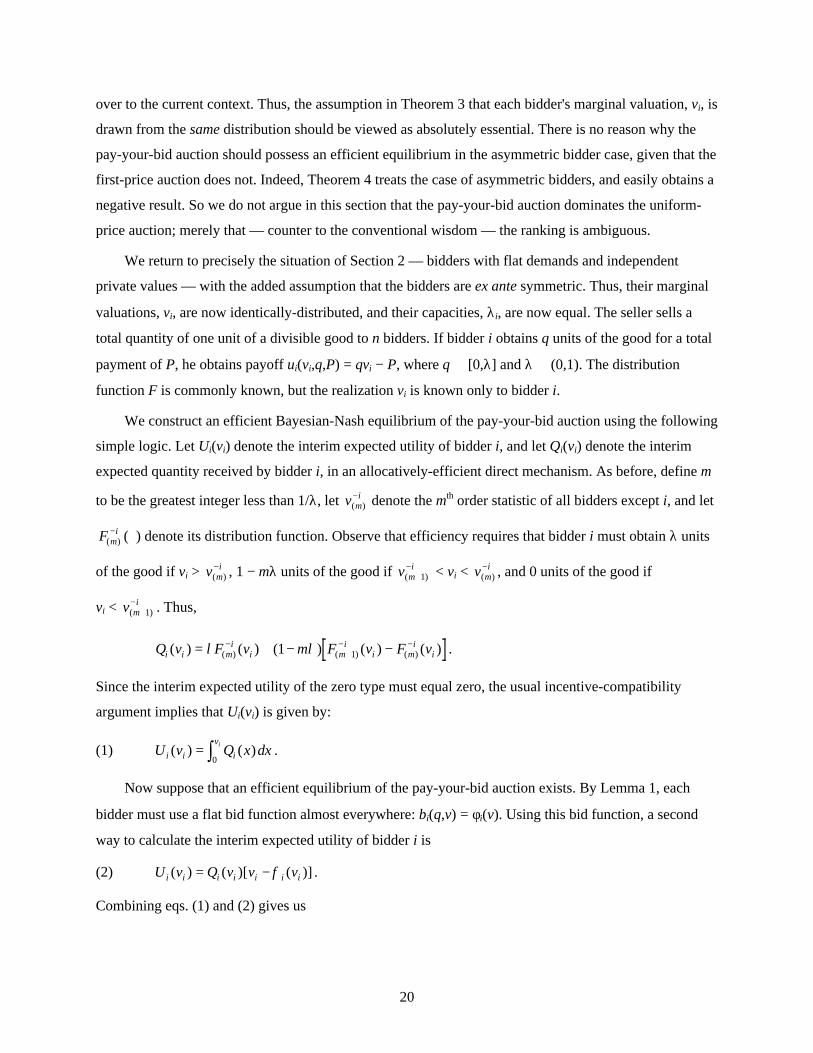
influence price and win a positive quantity. This provides an incentive for a bidder to bid below its
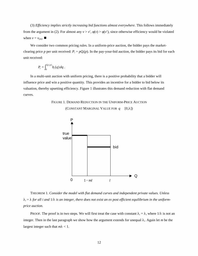
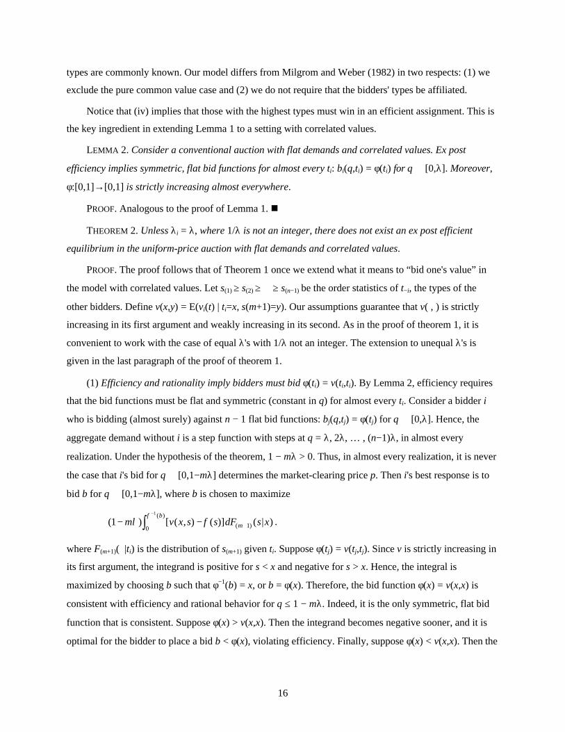
valuation, thereby upsetting efficiency. Figure 1 illustrates this demand reduction with flat demand
curves.
FIGURE 1. DEMAND REDUCTION IN THE UNIFORM-PRICE AUCTION
(CONSTANT MARGINAL VALUE FOR q ∈ [0,λ])
THEOREM 1. Consider the model with flat demand curves and independent private values. Unless
λi = λ for all i and 1/λ is an integer, there does not exist an ex post efficient equilibrium in the uniform-
price auction.
PROOF. The proof is in two steps. We will first treat the case with constant λi = λ, where 1/λ is not an
integer. Then in the last paragraph we show how the argument extends for unequal λi. Again let m be the
largest integer such that mλ < 1.
true value
bid
P
Q 0 1− mλ λ
13
(1) Efficiency and rationality imply bidders must bid their values. By Lemma 1, efficiency requires
that the bid functions must be flat (constant in q) for almost every vi. Consider a bidder i who is bidding
(almost surely) against n − 1 flat bid functions: bj(q,vj) = φ(vj) for q ∈ [0,λ]. Hence, the aggregate demand
without i is a step function with steps at q = λ, 2λ,… , (n − 1)λ, in almost every realization. Since 1/λ is
not an integer, 0 < 1−mλ < λ. Thus, in almost every realization, it is never the case that i's bid for
q ∈ [0,1−mλ] determines the market-clearing price p. Then i's best response is to maximize the
probability (and quantity) of winning whenever p ≤ vi. This is accomplished by bidding bi(q,vi) = vi for
q ∈ [0,1−mλ]. By bidding more than vi, i wins additional cases but pays a price p > vi in each of these
additional cases. By bidding less than vi, i loses some profitable cases where p < vi. But since efficiency
requires that the bid function be flat almost everywhere and rationality requires the bidder to bid its value
for q ∈ [0,1−mλ], then the only bid function consistent with efficiency and rationality is bi(q,vi) = vi for all
q ∈ [0,λ].
(2) Bidding one's value is not a best response to everyone else bidding their values. Suppose that all
bidders other than i are bidding their values: bj(q,vj) = vj for all q ∈ [0,λ] for j ≠ i. We wish to show that it
is not a best response for bidder i to bid bi(q,vi) = vi for all q ∈ [0,λ]. Consider an alternative strategy of
bidding bi(q,vi) = vi for q ∈ [0,1−mλ] and bi(q,vi) = b for q ∈ [1−mλ,λ], where b ≤ vi. Let πi(vi,b) be the
expected payoff from this two-step strategy given that the other firms are bidding their values. We wish to
show that dπi(vi,b)/db evaluated at b = vi is negative, which implies that bidder i can improve its payoff by
using the two-step bid function with b < vi, rather than bid its value for all q.
There are three regions of bidder valuations to consider in calculating πi(vi,b):
1. The mth highest valuation of the other bidders is less than b. Then bidder i wins λ and the price is
determined by the mth highest valuation. The contribution to the expected payoff is
λ ( ) ( )( )v p dF pi mib
− −z0 .
The derivative of this term with respect to b is 0 when evaluated at b = vi. Decreasing b decreases the
upper limit of integration, but the integrand is 0 when evaluated at b = vi.
2. b is between the mth highest valuation and the (m+1)st highest valuation of the other bidders. Then
bidder i wins 1 − mλ and b determines the price. The contribution to the expected payoff is
( )( )[ ( ) ( )]( ) ( )1 1− − −+− −m v b F b F bi m
im
iλ .
The derivative of this term with respect to b when evaluated at b = vi is
− − −+− −( )[ ( ) ( )]( ) ( )1 1m F v F vm
ii m
iiλ .
14
3. b is less than the (m+1)st highest valuation of the other bidders. Then when vi is greater than the
(m+1)st value, bidder i wins 1 − mλ and the (m+1)st value determines the price. When vi is less than the
(m+1)st value, bidder i wins zero units and obtains zero payoff. The contribution to the expected payoff is
( ) ( ) ( )( )1 1− − +−zm v p dF pi m
i
b
viλ .
The derivative of this term with respect to b is 0 when evaluated at b = vi. Decreasing b, decreases the
lower limit of integration, but again the integrand is 0 when evaluated at b = vi.
Collecting terms, we find dπi(vi,b)/db evaluated at b = vi is
− − − <+− −( )[ ( ) ( )]( ) ( )1 01m F v F vm
ii m
iiλ ,
for all vi ∈ (0,1), since each of the two terms in the product is positive. Hence, there exists b < vi such that
bidder i strictly gains by bidding b for q ∈ (1−mλ,λ], so it cannot be an equilibrium for each bidder to bid
its value. From (1) and (2), bidding one's value is the only candidate for an efficient equilibrium. Thus,
there cannot be an efficient equilibrium.
Finally, let us extend the above argument to unequal λi. Observe that the critical element in the
argument for equal λ was to show that the feasible interval [0,λ] could be divided into two nondegenerate
subintervals, with the property that the bidder was never pivotal for quantities in the low subinterval, but
that the bidder was pivotal with positive probability for quantities in the high subinterval. Then the bidder
would optimally bid her true value on the initial quantities, but could strictly gain by shading her bid on
the later quantities. With unequal λi, we will rank the bidders in descending order of capacity, and show
that the feasible interval [0,λ1] of the highest-capacity bidder can also be divided into two nondegenerate
subintervals, with the same property as before. Since not all λi are equal, it must be that λ1 > λn. Define
JI n
ii I
ii I
= <RST
UVW⊂ ∈ ∈∑ ∑arg max
{ , , }21
K
λ λ ,
and let S = ∑j∈J λj. J is the combination of bidders other than bidder 1 with an aggregate capacity, S,
closest to, but strictly less than, one (the total available). In every realization, bidder 1 will not be pivotal
on the quantity q ∈ [0,1−S), assuming that the other players use flat bid functions. Hence, bidder 1
optimally bids her true value for quantities q ∈ [0,1−S). By construction, 1 − S > 0. However, for
quantities greater than or equal to 1 − S, there is a positive probability that bidder 1 will be pivotal. Indeed
a lower bound on the probability that bidder 1 is pivotal at the quantity 1 − S is
Pr(vj > v1 ∀ j ∈ J)⋅Pr(vk < v1 ∀ k ∉ J). For any v1 ∈ (0,1), this probability is positive. Hence, for all
quantities above 1 − S, bidder 1 strictly gains by shading her bid. It remains to be shown that 1 − S < λ1,
15
so that there is a nondegenerate subinterval on which bidder 1 shades. Define i = max{j | j∉J}. Observe
that j > 1, since λ2 + … + λn ≥ 1. There are two cases: λi < λ1 (Case I); and λi = λ1 (Case II). In Case I,
consider the set J ∪ {i}. By the definition of S, we have S + λi ≥ 1. In Case II, observe that i ≠ n, so n ∈ J.
Consider the set J ∪ {i}\{n}. By the definition of S, we have S + λi − λn ≥ 1. In each case, this implies
that λ1 > 1 − S, as desired. We conclude that bidding her true value is not a best response for bidder 1, if
all other bidders are bidding their true values, excluding the possibility of an efficient equilibrium .n
The intuition behind Theorem 1 is that bidders have market power in the uniform-price auction. If a
bidder has a positive probability of influencing price in a situation where the bidder wins a positive
quantity, then the bidder has an incentive to shade its bid. This intuition is formalized in the proof. A
bidder's marginal gain from shading its bid is simply the quantity at which the bidder becomes pivotal
times the probability that the bidder is pivotal.
If λi = λ where 1/λ is an integer, then the proof does not go through. In this special case, if the other
bidders have flat bid functions, the quantity at which each bidder first becomes pivotal is zero. Since the
bidder only affects price when it wins nothing, bidding one's value is a best response and efficiency is
achieved. However, this is a knife-edge result. Efficiency is the exception, not the rule. Efficiency is lost
in essentially all settings outside of the unit demand case.
3 Inefficiency with Correlated ValuesThe inefficiency result does not require independent private values. Indeed, Theorem 1 extends to
Milgrom and Weber's (1982) setting, if we exclude the case of pure common values.
Let ti ∈ [0,1] be bidder i's type, t = (t1,…,tn), and t−i = t\ti. As before, denote the order statistics of t by
t(1) ≥ ⋅⋅⋅ ≥ t(n). Types are drawn from the symmetric joint distribution F with positive and finite density f on
[0,1]n. Bidder i's marginal value, vi(t):[0,1]n→ [0,1], satisfies:
(i) A higher type has a higher value: ∂vi(t)/∂ti > 0.
(ii) A higher type of another does not reduce one's value: ∂vi(t)/∂tj ≥ 0.
(iii) Type symmetry: ti = tj ⇒ vi(ti,t−i) = vj(tj,t−j).
(iv) Not common-value: ti > tj ⇒ vi(t) > vj(t).
In the private value model, vi only depends on ti, so the condition in (ii) is an equality. In the common
value model, (iii) is replaced with vi(t) = vj(t). Assumption (iv) assures that there is some private value
component. In a common-value setting, any assignment is efficient, so any auction without a reserve is
efficient. A bidder's type is private information; whereas, the value functions and the joint distribution of
16
types are commonly known. Our model differs from Milgrom and Weber (1982) in two respects: (1) we
exclude the pure common value case and (2) we do not require that the bidders' types be affiliated.
Notice that (iv) implies that those with the highest types must win in an efficient assignment. This is
the key ingredient in extending Lemma 1 to a setting with correlated values.
LEMMA 2. Consider a conventional auction with flat demands and correlated values. Ex post
efficiency implies symmetric, flat bid functions for almost every ti: bi(q,ti) = φ(ti) for q ∈ [0,λ]. Moreover,
φ:[0,1]→[0,1] is strictly increasing almost everywhere.
PROOF. Analogous to the proof of Lemma 1. n
THEOREM 2. Unless λi = λ, where 1/λ is not an integer, there does not exist an ex post efficient
equilibrium in the uniform-price auction with flat demands and correlated values.
PROOF. The proof follows that of Theorem 1 once we extend what it means to “bid one's value” in
the model with correlated values. Let s(1) ≥ s(2) ≥ ⋅⋅⋅ ≥ s(n−1) be the order statistics of t−i, the types of the
other bidders. Define v(x,y) = E(vi(t) | ti=x, s(m+1)=y). Our assumptions guarantee that v(⋅,⋅) is strictly
increasing in its first argument and weakly increasing in its second. As in the proof of theorem 1, it is
convenient to work with the case of equal λ's with 1/λ not an integer. The extension to unequal λ's is
given in the last paragraph of the proof of theorem 1.
(1) Efficiency and rationality imply bidders must bid φ(ti) = v(ti,ti). By Lemma 2, efficiency requires
that the bid functions must be flat and symmetric (constant in q) for almost every ti. Consider a bidder i
who is bidding (almost surely) against n − 1 flat bid functions: bj(q,tj) = φ(tj) for q ∈ [0,λ]. Hence, the
aggregate demand without i is a step function with steps at q = λ, 2λ, … , (n−1)λ, in almost every
realization. Under the hypothesis of the theorem, 1 − mλ > 0. Thus, in almost every realization, it is never
the case that i's bid for q ∈ [0,1−mλ] determines the market-clearing price p. Then i's best response is to
bid b for q ∈ [0,1−mλ], where b is chosen to maximize
( ) [ ( , ) ( )] ( | )( )
( )1 10
1
− − +
−zm v x s s dF s xm
bλ φ
φ.
where F(m+1)( ⋅|ti) is the distribution of s(m+1) given ti. Suppose φ(tj) = v(tj,tj). Since v is strictly increasing in
its first argument, the integrand is positive for s < x and negative for s > x. Hence, the integral is
maximized by choosing b such that φ−1(b) = x, or b = φ(x). Therefore, the bid function φ(x) = v(x,x) is
consistent with efficiency and rational behavior for q ≤ 1 − mλ. Indeed, it is the only symmetric, flat bid
function that is consistent. Suppose φ(x) > v(x,x). Then the integrand becomes negative sooner, and it is
optimal for the bidder to place a bid b < φ(x), violating efficiency. Finally, suppose φ(x) < v(x,x). Then the
17
integrand becomes negative later and it is optimal for the bidder to place a bid b > φ(x), again violating
efficiency. Hence, the only consistent bid function is φ(x) = v(x,x). But since efficiency requires that the
bid function be flat almost everywhere and rationality requires the bidder to bid v(x,x) for q ∈ [0,1−mλ],
then the only bid function consistent with efficiency and rationality is bi(q,ti) = v(ti,ti) for all q ∈ [0,λ].
(2) Bidding φ(x) = v(x,x) is not a best response to everyone else bidding φ(x) = v(x,x). Suppose that
all bidders other than i are bidding bj(q,tj) = φ(tj) for all q ∈ [0,λ] for j ≠ i. We wish to show that it is not a
best response for bidder i to bid bi(q,ti) = φ(ti) for all q ∈ [0,λ]. Consider an alternative strategy of bidding
bi(q,ti) = φ(ti) for q ∈ [0,1−mλ] and bi(q,ti) = b for q ∈ [1−mλ,λ], where b ≤ φ(ti). Let πi(ti,b) be the
expected payoff from this two-step strategy given that the other firms are bidding φ(tj). We wish to show
that dπi(ti,b)/db evaluated at b = φ(ti) is negative, which implies that bidder i can improve its payoff by
using the two-step bid function with b < φ(ti), rather than bid φ(ti) for all q.
As in Theorem 1, there are three regions of bidder valuations to consider in calculating πi(ti,b):
1. The mth highest type of the other bidders is less than φ−1(b). Then bidder i wins λ and the price is
determined by the mth highest bid of the others. The contribution to the expected payoff is
λφ
[ ( | , ) ( , )] ( | )( ) ( )
( )E v t s s v s s dF s ti i m m i
b= −
−z01
.
The derivative of this term with respect to b when evaluated at b = φ(ti) is
λφ φ− ′ = −1 ( ( ))[ ( | , ) ( , )]( )t E v t s t v t ti i i m i i i .
2. φ−1(b) is between the mth highest type and the (m+1)st highest type of the other bidders. Then
bidder i wins 1 − mλ and b determines the price. The contribution to the expected payoff is
( ) [ ( | , , ) ] ( , | )( ) ( )( )
( )1 1
1
0 1
1
− = = −+−
− zzm E v t s r s s b f r s t dr dsi i m m ib
bλ
φ
φ,
where f(⋅,⋅|ti) is the joint density of s(m) and s(m+1) given ti. The derivative of this term with respect to b
when evaluated at b = φ(ti) can be broken into two nonzero terms:
− − < <+( ) Pr( )( ) ( )1 1m s t sm i mλ , and
− − ′ = = −−+z( ) ( ( )) [ ( | , , ) ( )] ( , | )( ) ( )1 1
10m t E v t s t s s t f t s t dsi i i m i m i i i
tiλ φ φ φ ,
which simplifies to
− − ′ = −−( ) ( ( ))[ ( | , ) ( , )]( )1 1m t E v t s t v t ti i i m i i iλ φ φ .
18
The third term in the derivative evaluates to 0:
( ) ( ( )) [ ( | , , ) ( , )] ( , | )( ) ( )1 011
1− ′ = = − =−
+zm t E v t s r s t v t t f r t t dri i i m m i i i i iti
λ φ φ .
3. φ−1(b) is less than the (m+1)st highest type of the other bidders. Then when ti is greater than the
(m+1)st type, bidder i wins 1 − mλ and the (m+1)st type determines the price. The contribution to the
expected payoff is
( ) ( ( , ) ( , )) ( | )( )( )1 11
− − +−
−zm v t s v s s dF s ti mi
ib
tiλφ
.
The derivative of this term with respect to b is 0 when evaluated at b = φ(ti). Decreasing b, decreases the
lower limit of integration, but again the integrand is 0 when evaluated at b = φ(ti).
Collecting terms, we find dπi(ti,b)/db evaluated at b = φ(ti) is
− − < < − + − − = <+( ) Pr( ) (( ) )[ ( , ) ( | , )]( ) ( ) ( )1 1 1 01m s t s m v t t E v t s tm i m i i i i m iλ λ ,
for all ti ∈ (0,1), since the first term is negative and the second term is nonpositive. Hence, bidder i strictly
gains by bidding b < φ(ti) for q ∈ [1−mλ,λ], so it cannot be an equilibrium for each bidder to bid φ(ti).
From (1) and (2), bidding φ(ti) is the only candidate for an efficient equilibrium. Thus, there cannot be an
efficient equilibrium. n
The intuition behind Theorem 2 is roughly the same as in the independent private values case.
Bidders have market power, since they influence the price with positive probability. However, now a
bidder's marginal gain from shading its bid consists of two terms: (1) the quantity at which the bidder
becomes pivotal times the probability that the bidder is pivotal, and (2) the net winner's curse effect of
shading its bid.
4 The Ambiguous Ranking of the Pay-Your-Bid AuctionAs reviewed in the Introduction, it has often been claimed (especially in discussions of the U.S.
Treasury auctions) that the uniform-price auction is superior to the pay-you-bid auction for selling
multiple items. We have seen above that this intuition, which derives largely from the analysis of auctions
where bidders have tastes for only a single item, is substantially flawed: in uniform-price auctions,
rational bidders will bid strategically by submitting lower unit prices for larger quantities than for smaller
quantities, even in contexts where demands are flat.
In this section, we will go a step further by establishing the surprising result that in some fairly
reasonable situations where efficiency was impossible in a uniform-price auction, full efficiency is
nevertheless possible in a pay-your-bid auction. The intuition is quite straightforward. Our inefficiency
19
results were driven by the incentive for demand reduction in the uniform-price auction, which is the flip
side of the supply reduction by a monopolist or Cournot oligopolist: a bidder who shades her bids on
subsequent units saves money on the purchase of earlier units. By contrast, this incentive does not
literally exist in the pay-your-bid auction: a bidder who reduces her demand for subsequent units (but
holds her bids constant on earlier units) does not realize any savings on her purchase of earlier units. A
bidder's demand reduction may reduce the market-clearing price, but this provides no help to her other
purchases, which are made at the prices he bid.
To push the analogy further, consider the situation of a monopolist who can perform perfect price
discrimination. Recall that — mostly in the Treasury auction context — the uniform-price auction is often
referred to as a “nondiscriminatory auction” while the pay-you-bid auction is often referred to as a
“discriminatory auction.” Just as a monopoly without price discrimination leads to social inefficiency but
a monopoly with perfect price discrimination may realize all gains from trade, a nondiscriminatory
auction will lead to inefficiency but a discriminatory auction has the possibility of efficiency. The
explanation under monopoly is related to the auction result: the nondiscriminating monopolist's marginal
revenue curve lies strictly below her demand curve (except at a zero quantity); while the perfectly-
discriminating monopolist's marginal revenue curve may actually coincide with her demand curve. So we
obtain supply reduction in the former situation, but not necessarily in the latter situation.
Our discussion in this section emphasizes the goal of allocative efficiency. However, the ambiguous
ranking of the uniform-price and pay-your-bid auctions equally holds if the objective is maximizing the
seller's revenue. Our argument in Section 6 will establish that in the situation of symmetric bidders with
flat demands studied in this section, the efficient equilibrium of the pay-your-bid auction yields higher
expected seller revenues than any equilibrium of the uniform-price auction. The “optimal auction”
problem — subject to the constraint that the seller must dispose of all units — is solved by awarding all
units to the buyers who value them the most, i.e., optimality requires efficiency. The efficient equilibrium
of Theorem 3 thus also maximizes expected seller revenues. By contrast, application of Theorem 1
establishes that all Nash equilibria of the uniform-price auction yield strictly lower seller revenues. It is
thus possible to construct plausible demand structures such that the pay-your-bid format yields higher
expected seller revenues than the uniform-price format.
However, the positive result of Theorem 3 should not be taken too far. Consider the oft-studied
problem of the first-price auction for a single indivisible item. It is well known that very special
conditions are necessary for the first-price auction to admit an efficient equilibrium. Instead, if bidders'
valuations are random variables which are not identically distributed, then any equilibrium of the first-
price auction will typically be inefficient. These considerations from the first-price auction equally carry
20
over to the current context. Thus, the assumption in Theorem 3 that each bidder's marginal valuation, vi, is
drawn from the same distribution should be viewed as absolutely essential. There is no reason why the
pay-your-bid auction should possess an efficient equilibrium in the asymmetric bidder case, given that the
first-price auction does not. Indeed, Theorem 4 treats the case of asymmetric bidders, and easily obtains a
negative result. So we do not argue in this section that the pay-your-bid auction dominates the uniform-
price auction; merely that — counter to the conventional wisdom — the ranking is ambiguous.
We return to precisely the situation of Section 2 — bidders with flat demands and independent
private values — with the added assumption that the bidders are ex ante symmetric. Thus, their marginal
valuations, vi, are now identically-distributed, and their capacities, λi, are now equal. The seller sells a
total quantity of one unit of a divisible good to n bidders. If bidder i obtains q units of the good for a total
payment of P, he obtains payoff ui(vi,q,P) = qvi − P, where q ∈ [0,λ] and λ ∈ (0,1). The distribution
function F is commonly known, but the realization vi is known only to bidder i.
We construct an efficient Bayesian-Nash equilibrium of the pay-your-bid auction using the following
simple logic. Let Ui(vi) denote the interim expected utility of bidder i, and let Qi(vi) denote the interim
expected quantity received by bidder i, in an allocatively-efficient direct mechanism. As before, define m
to be the greatest integer less than 1/λ, let v mi
( )− denote the mth order statistic of all bidders except i, and let
F mi
( )− ( ⋅) denote its distribution function. Observe that efficiency requires that bidder i must obtain λ units
of the good if vi > v mi
( )− , 1 − mλ units of the good if v m
i( )+−
1 < vi < v mi
( )− , and 0 units of the good if
vi < v mi
( )+−
1 . Thus,
Q v F v m F v F vi i mi
i mi
i mi
i( ) ( ) ( ) ( ) ( )( ) ( ) ( )= + − −−+
− −λ λ1 1 .
Since the interim expected utility of the zero type must equal zero, the usual incentive-compatibility
argument implies that Ui(vi) is given by:
(1) U v Q x dxi i i
vi( ) ( )= z0 .
Now suppose that an efficient equilibrium of the pay-your-bid auction exists. By Lemma 1, each
bidder must use a flat bid function almost everywhere: bi(q,v) = φi(v). Using this bid function, a second
way to calculate the interim expected utility of bidder i is
(2) U v Q v v vi i i i i i i( ) ( )[ ( )]= − φ .
Combining eqs. (1) and (2) gives us
21
(3) φ i i i
i
v
i i
v vQ x dx
Q v
i
( )( )
( )= − z0 .
We thus have
THEOREM 3. If bidders' valuations are i.i.d. and their capacities, λi, are equal, then eq. (3) provides
an ex post efficient equilibrium of the pay-your-bid auction.
PROOF. The above argument showed that a necessary condition for an ex post efficient equilibrium
of the pay-your-bid auction is eq. (3). If vi and vj are i.i.d. and λi = λj, then Qi(⋅) = Qj(⋅) and
φi(⋅) = φj(⋅) ≡ φ(⋅). Furthermore, φ(⋅) is strictly monotone increasing, so every bidder using the same bid
function, φ(⋅), leads to an efficient allocation. Finally, it is easily verified that every bidder using φ(⋅)
constitutes a Bayesian-Nash equilibrium. n
Observe that Theorem 3 placed no restriction on λ. By way of contrast, recall that Theorem 1
permitted an efficient equilibrium in the uniform-price auction only if 1/λ equaled an integer. Thus, the
two theorems together generate a continuum of reasonable situations where the symmetric, constant-bid
equilibrium of the pay-your-bid auction outperforms every equilibrium of the uniform-price auction on
efficiency. (See Example 4.3 below.) Theorem 6 will further show that this equilibrium of the pay-your-
bid auction outperforms every equilibrium of the uniform-price auction on seller revenues.
It is not difficult to generate examples for which the efficient pay-your-bid equilibrium has a closed
form. We provide two examples.
EXAMPLE 4.1. n = 3, λ = 0.6. F(⋅) is the uniform distribution on [0,1]. Then the efficient equilibrium
bid function is
φ( )vv
vv=
−−
FHG
IKJ
6 2
12 3.
EXAMPLE 4.2. “The 2½-Item Auction.” n = 4, λ = 0.4. F(⋅) is the uniform distribution on [0,1]. Then
the efficient equilibrium bid function is
φ( )vv
vv=
−−
FHG
IKJ
6 3
12 4
2
2 .
The above reasoning also allows us to easily obtain a negative result for the case of asymmetric
bidders.
22
THEOREM 4. If bidders' valuations are independent but not identically distributed, or if their
capacities are unequal, then generically there does not exist an ex post efficient equilibrium of the pay-
your-bid auction.
PROOF. Suppose there exist bidders i and j such that the associated distribution functions, Fi(⋅) and
Fj(⋅), are not identical. As before, a necessary condition for an ex post efficient equilibrium is that bidder
i's bid function be given by φi(⋅), defined by the right-hand-side of (3). At the same time, another
necessary condition is that bidder j's bid function be given by φj(⋅), defined by replacing F mi
( )− and F m
i( )+−
1
with F mj
( )− and F m
j( )+−
1 in the right-hand-side of (3). For generic Fj ≠ Fi, the implied φj ≠ φi on sets of
positive measure, contrary to Lemma 1. We conclude that there cannot exist any ex post efficient
equilibrium.
Similarly, if the capacities λi are not all equal, then eq. (3) again implies that, if λj ≠ λi, then φj ≠ φi
on sets of positive measure. Hence, there again cannot exist an ex post efficient equilibrium. n
Using the results we have developed thus far, it can be shown that the efficiency ranking of the
uniform-price and pay-your-bid auctions is inherently ambiguous. Applying Theorem 6, below, to
Example 4.3 will also show that the pay-your-bid auction can dominate the uniform-price auction in
revenue terms, providing a counterexample to Friedman's conjecture, and that the Vickrey auction can in
turn revenue-dominate the standard auction formats. Finally, Theorem 6 is stated more generally to allow
for reserve prices, so analogous revenue rankings can be made for these same auction formats with
appropriately-chosen reserve prices.
EXAMPLE 4.3. VICKREY f PAY-YOUR-BID f UNIFORM-PRICE.
Consider the flat demands model. Start with i.i.d. vi, and start with capacities λi ≡ λ (∀i), where 1/λ is not
an integer. Then perturb the capacities, λi, to make them slightly unequal.
Before the perturbation, Theorems 1 and 3 implied that Vickrey ~ Pay-Your-Bid f Uniform-Price,
in efficiency terms. By Theorem 4, any perturbation which makes the capacities unequal renders Vickrey
f Pay-Your-Bid; for a sufficiently small perturbation, we also maintain Pay-Your-Bid f Uniform-Price,
where the comparison is between the symmetric, constant-bid equilibrium of the pay-your-bid auction and
all equilibria of the uniform-price auction.
Using Theorem 6, below, this is a model where allocative efficiency coincides with revenue
maximization. Thus, it can easily be seen that this same example provides the same ranking in terms of
seller revenues.
EXAMPLE 4.4. VICKREY f UNIFORM-PRICE f PAY-YOUR-BID.
23
Consider the flat demands model. Start with i.i.d. vi, and start with capacities λi ≡ λ (∀i), where 1/λ equals
an integer. Perform two perturbations in succession. First, perturb the distribution functions so as to no
longer be identically distributed. Then perturb the capacities, λi, to make them slightly unequal.
Before either perturbation, Theorem 3 implied that Vickrey ~ Uniform-Price ~ Pay-Your-Bid, in
efficiency terms (where we select the efficient equilibrium of each auction). By Theorem 4, the first
perturbation renders Vickrey f Pay-Your-Bid; but sincere bidding remains an equilibrium of the
uniform-price auction, so Vickrey ~ Uniform-Price. By Theorem 1, any perturbation which makes the
capacities unequal renders Vickrey f Uniform-Price; for a sufficiently small perturbation, we also
maintain Uniform-Price f Pay-Your-Bid.
5 Inefficiency with Downward-Sloping DemandsIn the preceding sections, we considered uniform-price auctions when bidders possessed a severe
version of diminishing marginal values for the items at auction. Bidder i's marginal values were constant
over quantities qi ∈ [0,λi], but then discontinuously dropped to zero for quantities qi ∈ (λi,1]. In this
section, we reconsider the inefficiency argument when bidders' marginal values are smoothly decreasing
in quantity. We find that inefficiency is still mandated in the uniform-price auction, and that perhaps the
intuition is clearer than in the flat demand case.
Let ti denote the type of bidder i. As in Section 2, the types {t1,…,tn} are drawn independently
according to the distribution functions {F1,…,Fn}, respectively, where each Fi has positive and finite
density fi on a support of [0,1]. Each distribution function Fi is commonly known, but the realization ti is
known only to bidder i. If type ti of bidder i obtains x ∈ [0,1] units of the good for a total payment of P,
her payoff is given by Vi(x,ti) − P . The valuation functions, Vi(⋅,⋅), are required to have continuous partial
derivatives with respect to x, which we denote by vi(⋅,⋅). We make the following assumptions on the
marginal value functions vi(⋅,⋅), for i = 1,…,n:
(4) vi(⋅,⋅) is continuous in its two arguments and has continuous partial derivatives in each;
(5) vi(0,ti) = ti, for all ti ∈ [0,1];
(6) vi(x,0) = 0, for all x ∈ [0,1];
(7) ∂vi(x,ti)/∂ti ≥ 0, for all ti ∈ [0,1] and for all x ∈ [0,1];
(8) ∂vi(x,ti)/∂x ≤ 0, for all ti ∈ [0,1] and for all x ∈ [0,1].
In addition, we require that at least one bidder j, j ∈ {1,…,n}, satisfy:
(7′) ∂vj(x,tj)/∂tj > 0, for all tj ∈ [0,1] and for all x ∈ [0,1];
24
(8′) ∂vj(x,tj)/∂x < 0, for all tj ∈ (0,1] and for all x ∈ [0,1].
Thus, marginal value is weakly increasing (strictly for at least one bidder) in type, and type has the literal
interpretation of the bidder's marginal value at zero units. Furthermore, each type exhibits weakly
decreasing (strictly for nonzero types of at least one bidder) marginal value in quantity.
As before, our approach shall be to suppose that there exists an equilibrium in the uniform-price
auction which attains efficiency, and to demonstrate that this supposition leads to a contradiction. Taking
a mechanism-design approach, let us suppose that a mediator were to ask every bidder j, j ≠ i: “What
quantity, xj(v;tj), gives you a marginal value of v?” Let us suppose further that all bidders j, j ≠ i, respond
truthfully to this question. Finally, the mediator uses these responses together with the response of bidder
i (which is not assumed to necessarily be truthful) to attempt to allocate all the available (q = 1) units of
the good, according to the criterion of efficiency.
Let G−i(v;y) denote the probability that, under truthtelling by all bidders j, j ≠ i, and under efficient
allocation by the mediator, an order by bidder i for quantity y at a reported marginal value of v is filled.
To be precise,
(9) G v y x v t yij j
j i
−
≠
= ≤ −∑( ; ) Pr{ ( ; ) }1 .
Note that the function, G−i(v;y), is determined solely by the bidders' marginal values and the distribution
of bidders' types; it asks what is the probability of a particular order being filled if other bidders report
honestly and if the mediator carries out the allocation which appears efficient (taking all bidders' reports
literally).
Consider a uniform-price auction, and let bi(x,ti) denote the bid (the price per unit) submitted by type
ti of bidder i for quantity x. As in Section 2, we require the bids bi(⋅,ti):[0,1]→[0,1] to be right-continuous
and weakly-decreasing functions of x. Analogous to Lemma 1 above, we have
LEMMA 3. In any ex post efficient equilibrium of the uniform-price auction, bids are a strictly
monotone function of marginal value whenever G−i(x,ti) ∈ (0,1), i.e.,
(10) bi(x,ti) = φ(vi(x,ti)), where φ:[0,1]→[0,1] is strictly monotone.
The intuition for Lemma 3 is that, in a uniform-price auction (or any conventional auction), units of the
good are allocated to the highest bids. In order for the auction to place the goods in the hands who value
them most, bids for any given quantity must be monotone in the marginal value. The meaning of
G−i(v,y) ∈ (0,1) is simply that we are not speaking about a bid which is sure to win or sure to lose;
changes in rankings of such bids have no effect on either the allocation or the payment in a uniform-price
auction, so monotonicity in value is unnecessary there.
25
Now let us assume that φ(⋅) defined by (10) is continuously differentiable,5 and let us derive the
Euler equation expressing the requirement that bidder i is optimizing in her quantity, y(v), ordered for
each v. The problem for type ti of bidder i is to determine the function y(v) which maximizes her expected
payoff:
(11) max { ( , ) ( ) } ( ; )( )y
i iV y t v y dG v y⋅
∞−z φ
0,
where, for notational brevity, we have now dropped the superscript “−i” from G−i(v;y). Integrating by
parts, (11) may be rewritten:
(12) max { ( ) [ ( , ) ( )] } ( ; )( )y
i iv y v y t v y G v y dv⋅
∞′ − − ′z φ φ
0.
Thinking of the integrand in (12) as a function of v, y(v), and y′(v), we can characterize the solution to this
maximization problem by the following Euler equation:
(13) [ ( , ) ( )] ( ; ) ( ) ( ; )v y t v G v y y v G v yi i v y− + ′ =φ φ 0 .
where Gv(v;y) and Gy(v;y), respectively, denote the partial derivatives of G(v;y), defined in (9), with
respect to v and y.6 Observe that our Euler equation is virtually the same as that of Wilson (1979, p. 681),
except that: (1) we treat y(⋅) as a function of v (whereas Wilson uses y(⋅) as a function of p); and (2) our
probability G(v;y) is defined with respect to the efficient allocation rule (whereas Wilson's H(p;v,y) is
defined with respect to an equilibrium allocation rule).
Moreover, we still need to impose the additional requirement that bidder i report truthfully.7 For the
outcome to be efficient, it must be the case that truthtelling satisfies the Euler equation (13) for bidder i.
Substituting xi(v;ti) in place of y, in (13) yields:
(14) [ ( )] ( ; ( ; )) ( ; ) ( ) ( ; ( ; ))v v G v x v t x v t v G v x v tv i i i i y i i− + ′ =φ φ 0 .
We also require
LEMMA 4. Assume that every bidder i, i = 1,…,n, satisfies conditions (4)–(8), and at least one bidder
j, j ≠ i, also satisfies (7′)-(8′). Then for every (v,y) such that G−i(v,y) ∈ (0,1):
5 While the assumption that the bid function is continuously differentiable does not seem to be an especially strongassumption in this game, the authors suspect that the continuous-differentiability assumption is probablyunnecessary, and that the proof that equilibria of the uniform-price auction are inefficient can be replicated when bidfunctions are merely assumed to be weakly-decreasing, right-continuous, measurable functions of quantity.6 For a general derivation of the Euler equation, see, for example, Luenberger (1969) pp. 179-81.7 We have so far only assumed that all other bidders reveal truthfully and that the allocation is done efficiently givenall reports.
26
(15) G v yvi− ( ; ) > 0 , and
(16) G v yyi− ( ; ) < 0 .
PROOF. First, consider the case where n = 2. Then G−i(v,y) = Fj[tj(v;1−y)], where tj(v;z) is defined
implicitly by vj(z,tj(v;z)) = v (i.e., tj(v;z) denotes the type who has marginal value v when consuming z
units). By the implicit function theorem, and using (7′)-(8′), ∂tj(v,z)/∂v > 0 and ∂tj(v,z)/∂z > 0 whenever
G−i(v,z) ∈ (0,1). Thus, using the fact that the density is positive and bounded everywhere in the support,
G v yvi− ( ; ) = fj[tj(v;1−y)] ∂tj(v,1−y)/∂v > 0 and G v yy
i− ( ; ) = −fj[tj(v;1−y)]∂tj(v,1−y)/∂(1−y) < 0.
Second, we will establish the inductive step: if G v yvi− ( ; ) > 0 and G v yy
i− ( ; ) < 0 when there are m − 1
other bidders, then the same inequalities hold when there are m other bidders. Define:
G v y x v t ymj j
jj i
m−
=≠
−
= ≤ −∑1
1
1
1( ; ) Pr{ ( ; ) } and G v y x v t ymj j
jj i
m
( ; ) Pr{ ( ; ) }= ≤ −=≠
∑ 11
.
Observe that
(17) G v y G v y x v t f t dtm mm m m
t v ym( ; ) ( ; ( ; )) ( )
( ; )= +−−z 1
0
1.
Differentiating (17) with respect to each of v and y, and using the hypothesis that G v yvm−1( ; ) > 0 and
G v yym−1( ; ) < 0, allows us to conclude that G v yv
m ( ; ) > 0 and G v yym ( ; ) < 0.
By induction, we conclude that inequalities (15) and (16) hold when G−i(v,y) is calculated using all
n − 1 other bidders. n
We are now ready to prove
THEOREM 5. Assume that every bidder i = 1,…,n, satisfies conditions (4)–(8) and at least one bidder
j ∈ {1,…,n} also satisfies (7′)–(8′). Then there does not exist an ex post efficient equilibrium in the
uniform-price auction.
PROOF. Suppose instead that an efficient equilibrium exists. Select any i ≠ j, and consider any
v0 ∈ (0,1) with the property that G−i(v0,0) < 1. Such a v0 clearly exists under (7′)–(8′), and each v ∈ (0,v0)
has this same property. Observe that Lemma 4 implies that G vvi− ( ; )0 > 0 and G vy
i− ( ; )0 < 0 whenever
v ∈ (0,v0). We showed above that a necessary condition for an efficient equilibrium is the Euler equation
(14). For each v ∈ (0,v0), we can substitute (v,ti) = (v,v) into (14). Noting that xi(v;v) = 0, we conclude that
φ(v) = v for all v ∈ (0,v0).
27
However, we may instead substitute any v ∈ (0,v0) paired with any ti ∈ (v,1] into (14). Since
xi(v;ti) > 0, φ′(v) = 1, and G v x v tyi
i i− ( ; ( ; )) < 0, the second term of (14) is strictly negative. In order to offset
this, the first term of (14) would need to be strictly positive. Given that G v x v tvi
i i− ( ; ( ; )) > 0, this would
require [v − φ(v)] > 0. But we had already concluded that φ(v) = v, yielding a contradiction to our
hypothesis that there existed an efficient equilibrium. n
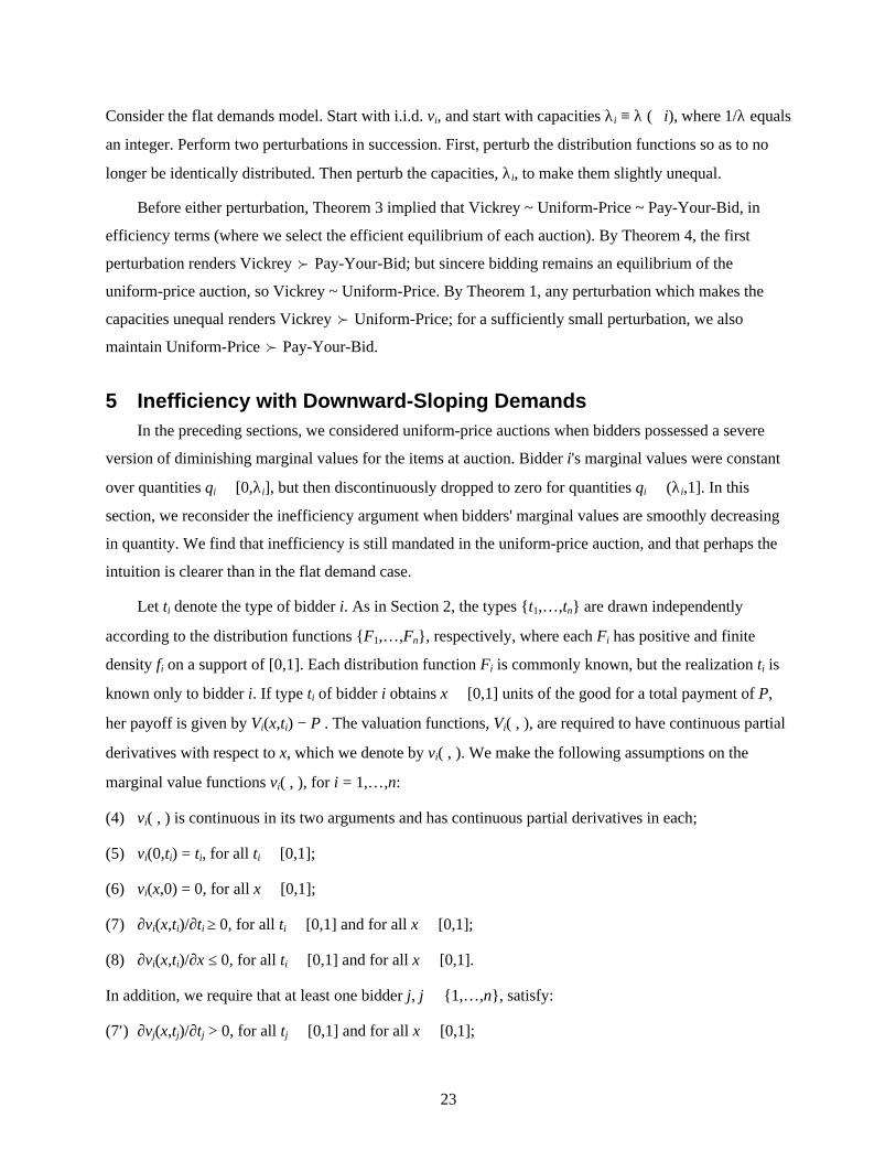
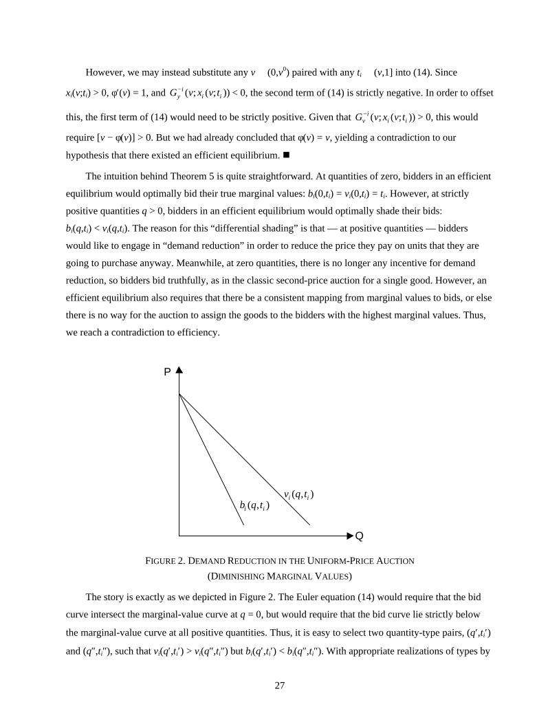
The intuition behind Theorem 5 is quite straightforward. At quantities of zero, bidders in an efficient
equilibrium would optimally bid their true marginal values: bi(0,ti) = vi(0,ti) = ti. However, at strictly
positive quantities q > 0, bidders in an efficient equilibrium would optimally shade their bids:
bi(q,ti) < vi(q,ti). The reason for this “differential shading” is that — at positive quantities — bidders
would like to engage in “demand reduction” in order to reduce the price they pay on units that they are
going to purchase anyway. Meanwhile, at zero quantities, there is no longer any incentive for demand
reduction, so bidders bid truthfully, as in the classic second-price auction for a single good. However, an
efficient equilibrium also requires that there be a consistent mapping from marginal values to bids, or else
there is no way for the auction to assign the goods to the bidders with the highest marginal values. Thus,
we reach a contradiction to efficiency.
FIGURE 2. DEMAND REDUCTION IN THE UNIFORM-PRICE AUCTION
(DIMINISHING MARGINAL VALUES)
The story is exactly as we depicted in Figure 2. The Euler equation (14) would require that the bid
curve intersect the marginal-value curve at q = 0, but would require that the bid curve lie strictly below
the marginal-value curve at all positive quantities. Thus, it is easy to select two quantity-type pairs, (q′,ti′)
and (q″,ti″), such that vi(q′,ti′) > vi(q″,ti″) but bi(q′,ti′) < bi(q″,ti″). With appropriate realizations of types by
Q
P
v q ti i( , )b q ti i( , )
28
the opposing bidders, this makes it impossible for the uniform-price auction to always place units in the
hands who value them the most.
6 Avoiding Demand Reduction: The Vickrey AuctionOur results in Sections 2 and 5 demonstrate that, in private-value auctions where bidders have tastes
for multiple items and exhibit diminishing marginal values, demand reduction and inefficiency are
endemic in uniform-price auctions. Section 4 showed for pay-your-bid auctions that efficiency was in
principle possible, but this required symmetry among bidders. The question remains as to whether auction
rules other than uniform-price or pay-your-bid are more amenable to efficiency. This section reviews the
Vickrey (1961) auction, which generates full efficiency when bidders have private values.
Consider either of the private-value situations treated in Sections 2, 4 and 5. As before, bidders in the
Vickrey auction simultaneously and independently submit sealed bids consisting of demand functions to
the auctioneer, who apportions units to the highest bidders but assigns payments neither according to a
uniform-price nor according to a pay-your-bid formula. Instead, the principle followed is that the price
paid for each unit equals the value of the bid which it displaces. In the case of M indivisible items, this
means that a bidder who wins K items pays the amount of the kth highest rejected bid other than her own
for the kth item (k = 1,…,K) she wins.
To be precise for the continuous treatment of this paper (i.e., the case of a perfectly-divisible item),
let xi(p) denote the quantity demanded by bidder i at a price p, and require each xi(⋅) to be a left-
continuous and weakly-decreasing function. Let x−i(p) denote the aggregate demand of all other bidders:
(18) x p x pi jj i
−≠
= ∑( ) ( ) .
Normalizing the supply of the item to equal one and observing that x−i(⋅) is also a left-continuous and
weakly-decreasing function, let us define
(19) p p x p x pi i0 1= + ≤−inf{ | ( ) ( ) } and p p x pi
i−
−= ≤inf{ | ( ) }1 .
(If the market does not clear at p0, then the quantity allocated to bidders is rationed as in Section 2.) Thus,
p0 denotes the market-clearing price, while p−i denotes the market-clearing price if bidder i had been
absent from the auction. The Vickrey auction awards a quantity of xi(p0) to bidder i, and requires a
payment denoted Pi, where
(20) P x p p x r dri i ip
p
i= − − −−z( ) { ( )}0 0 1
0
.
29
FIGURE 3. PAYMENT RULE IN VICKREY AUCTION
More intuitively, the outcome for bidder i in the Vickrey auction is depicted in Figure 3. The payment, Pi,
is the area under the {1 − x−i(p)} curve, from 0 to xi(p0), which is shaded in the figure. Thus, each
participant's payment (conditional upon winning a given quantity) is independent of her own bids,
circumventing any incentive for demand reduction.
Sincere bidding is a particularly compelling outcome in the Vickrey auction. Indeed, it is well known
that, with private values, sincere bidding is a weakly-dominant strategy, and that a single round of
elimination of weakly-dominated strategies gets rid of all strategies except for sincere bidding. Thus, a
Vickrey auction is especially conducive to efficiency.
However, most of the mechanism design literature devoted to auctions (e.g., Myerson 1981) has
focused not on the criterion of allocative efficiency, but rather on the objective of maximizing the seller's
expected revenues. In this light, the following theorem is especially reassuring. In an ex ante symmetric
setting with flat demand curves, the revenue-maximizing seller assigns the good to the bidders with the
highest values. Seller revenue is thus maximized by a Vickrey auction with a reserve price. We say that
the probability distribution F is regular if J(vi) ≡ vi − [1 − F(vi)]/f(vi) is strictly increasing in vi. We have:
THEOREM 6. Consider an incentive compatible and individually rational mechanism in which the
lowest-type bidder receives an expected payoff of zero. The seller's expected revenue is completely
determined by the allocation rule mapping types to quantities (i.e., the weak form of revenue equivalence
holds). Moreover, if the bidders have flat demand curves and the bidders' types are drawn independently
from the same regular distribution, then the seller's expected revenue is maximized by awarding the good
to those with the highest values, subject to the reserve price r which solves r = [1 − F(r)]/f(r). If the seller
Q
P
p0
p i−x pi ( )
1− −x pi ( )
30
is constrained to distribute all units of the good (i.e., constrained to set a reserve price of zero), then the
seller's expected revenue is maximized by using the efficient allocation rule.
PROOF. Let v ≡ (v1,…,vn) denote the vector of bidders' types. The weak form of revenue equivalence
follows from Proposition 2 of Maskin and Riley (1989).8 In particular, they show that the expected
revenue from an allocation {q1(v),…,qn(v)}, where type 0 has an expected payoff of 0, is:
(21) E q vF v
f vi ii
ii
n
v v( )( )
( )−
−FHG
IKJ
LNMM
OQPP=
∑ 1
1
.
Hence, the seller's optimization problem is to select an allocation rule {q1(v),…,qn(v)} to maximize
(21), where for all v, qi(v)∈ [0,λi], and ∑i qi(v)≤ 1. This problem is trivially solved by pointwise
optimization. Fix v. Since F is regular, vi − (1 − F(vi))/f(vi), is an increasing function of vi. Thus, the seller
should allocate the good to those with the highest values, until quantity is exhausted or the reserve price r
is reached. If the seller is constrained to sell all units (a reserve price of zero), then the seller does best by
assigning the good to those with the highest values until quantity is exhausted. n
Theorem 6 identifies the revenue maximizing assignment both with and without a constraint to sell
all units. More generally, for whatever quantity the seller chooses to sell, as a function of the bidders'
revealed types, the seller does best by awarding the good to those with the highest values. The only
distortion away from efficiency in the seller's optimal auction is the truncation of sales below the reserve
price r. Even this distortion is eliminated if we make the more realistic assumption that the set of bidders
is not fixed, but varies based on the bidders' rational decisions to participate (Harstad 1990, 1993, and
Levin and Smith 1994). An attempt by the seller to extract additional revenues by setting a positive
reserve discourages participation, which ultimately reduces revenues. Moreover, even if the seller wished
to set a binding reserve price, the Coase (1972) conjecture about the durable goods monopolist can be
reinterpreted to argue that the seller cannot credibly commit to holding back quantity.
Unfortunately, Theorem 6 does not generalize to the case of downward-sloping demand curves.
Maskin and Riley (1989) determine the optimal selling procedure in this case (their Proposition 5) and it
typically does not result in an efficient assignment. The optimal selling procedure assigns the good based
on the bidders' virtual demand curves (using Myerson's terminology); whereas, an efficient auction
assigns the goods based on the actual demand curves. With flat demands, the assignments based on actual
8 Revenue equivalence, as stated here, is extremely general. It does not depend on ex ante symmetry or even a one-dimensional type space (see Engelbrecht-Wiggans, 1988). Essentially, all that is required is a connected type space.Note that we are using the term revenue equivalence to mean that interim payoffs only depend on the assignment ofthe good, and hence any mechanisms that result in the same assignment must generate the same revenue, if the zerotype gets zero.
31
and virtual demands are identical in the symmetric, regular case. However, with downward sloping
demands, this need not be the case.
Whether the revenue-maximizing assignment distorts the efficient assignment depends on the
distribution of uncertainty. Suppose the bidders have inverse demands of pi(qi) = vi − gi(qi), where
dgi/dqi > 0 for all qi. Further suppose each vi is i.i.d. from the exponential distribution,
F(vi) = 1 − exp(−vi/α). In what follows we extend the support of vi to [0,∞). In this setting, the seller again
optimally assigns the good to those with the highest values:
THEOREM 7. Consider the model with downward-sloping demands and symmetric exponential
uncertainty. Then the seller's expected revenue is maximized by awarding the good to those with the
highest values subject to a reserve price r = α. If the seller is constrained to distribute all units of the
good (i.e., constrained to set a reserve price of zero), then the seller's expected revenue is maximized by
using the efficient allocation rule.
PROOF. The proof follows from Proposition 2 in Maskin and Riley (1989). In particular, they show
that the seller's expected revenue from an allocation {q1(v),…,qn(v)}, where type 0 has an expected payoff
of 0, is
E v g xF v
f vdxi i
i
i
q
i
ni
v
v− −
−LNM
OQP
FHG
IKJ
LNMM
OQPPz∑
=
( )( )
( )
( ) 10
1
.
However, since F is the exponential distribution, [1 − F(vi)]/f(vi) = α. Hence, the seller's optimization
problem is to select an allocation rule {q1(v),…,qn(v)} to maximize
(22) E v g x dxi i
q
i
ni
v
v− −FH IK
LNM
OQPz∑
=
( )( )
α0
1
,
where for all v, qi(v)∈ [0,1], and ∑i qi(v)≤ 1. By pointwise optimization, the solution to maximizing (22)
is to assign the good to those with the highest values subject to the reserve price r = α, or if constrained to
sell all units, the seller simply assigns the good to those with the highest values. n
For all distributions other than the exponential distribution, there is a conflict between revenue
maximization and efficiency, with downward-sloping demands. How revenue maximization distorts the
efficient assignment depends on the hazard rate of the distribution of uncertainty. For example, with
uniform uncertainty (an increasing hazard rate), virtual demands by lower types are shifted down more
than for higher types. Hence, the revenue-maximizing assignment differs from an efficient assignment by
shifting quantity away from the low-demand bidders (low types). With a decreasing hazard rate, the seller
increases revenues by shifting the good toward the low-demand bidders.
32
Recall that a uniform price auction tends to shift quantity toward small bidders, because of greater
demand reduction by large bidders. Hence, this suggests that, with ex ante symmetric bidders, an efficient
auction will generally revenue-dominate the uniform price auction whenever the hazard rate for the
distribution of uncertainty is nondecreasing. However, when there are ex ante asymmetries among the
bidders, then it would seem possible for the uniform-price auction to yield more revenue than an efficient
auction. For example, if there are a number of ex ante weak bidders (low demands), then competition may
be stimulated in an auction that gives these weak bidders more favorable treatment. The uniform-price
auction effectively does just that. Participation by small bidders is encouraged, since they win larger
quantities due to demand reduction by the stronger bidders. In general, “optimal” auctions take advantage
of any ex ante asymmetries among bidders, the precise shape of demand curves, and the distribution of
uncertainty.
7 An Efficient Ascending-Bid DesignGiven that the Vickrey auction is both allocatively efficient and optimal for the seller when bidders
have private values, the question remains as to why we do not observe the Vickrey design in practice for
multiple-item auctions. Two hypotheses may be put forward. First, the common-value component to
valuations may be sufficiently important that the gain to the seller from an ascending-bid design over
Vickrey's sealed-bid design more than offsets the loss arising from demand reduction in the uniform-
price, ascending-bid auction. Second, it may simply be the case that the Vickrey auction is believed to be
too complex for practitioners to understand.
This section briefly discusses an ascending-bid auction design, proposed in Ausubel (1997), which
replicates the (sealed-bid) Vickrey auction when bidders have private values. The alternative, ascending-
bid design may offer distinct advantages over the uniform-price, ascending-bid design when bidders have
private values, since our previous analysis identifies demand specifications such that the alternative
auction possesses an equilibrium which dominates all equilibria of the uniform-price auction (both in
terms of allocative efficiency and seller optimality). The ascending-bid design may also offer the seller
advantages over the standard Vickrey auction when bidders receive affiliated signals, for reasons
analogous to why the seller prefers the English auction to the sealed-bid auction when bidders receive
affiliated signals in the single-indivisible-item context. Finally, the payment rule in the ascending-bid
design should be much more transparent to practitioners than the black box of the Vickrey auction; as
claimed in Ausubel (1997), “the proposed ascending-bid auction design is simple enough to be
understood by any aficionado of baseball pennant races and the like.”
We allow the auctioneer to raise the price continuously, from an initial price of zero, in the style of
an ascending-clock auction. Bidder i's bidding strategy, denoted bi(p,Hi(p)), is a function of both the
33
current price, p, and the history, Hi(p), which is observable to bidder i. The history, Hi(p), observable to
bidder i is some summary of all bidders' realized demands at prices in the half-open interval [0,p).
We shall focus on the situation of Full Bid Information: the history, Hi(p), observable to bidder i
consists of the complete history of previous demand submissions of all bidders at all prices in the half-
open interval [0,p).9 Under the alternative assumption of No Bid Information — bidder i's observable
history consists only of her own previous demand submissions and the fact that the auction is still open —
the strategic options of each bidder are basically equivalent to those in the (sealed-bid) Vickrey auction.
Finally, bidders' submitted demands will be constrained to be right-continuous and weakly-decreasing in
price.
Let {x1(p),…,xn(p)} denote the actual submitted demands of all bidders, parameterized by price (until
the auction closes). Then the allocations and payments of all bidders will be determined exactly as in the
description of the Vickrey auction in Section 6. Thus, the market-clearing price equals p0 of eq. (19).
Bidder i wins a quantity of xi(p0), and is obliged to make a payment of Pi, defined in eq. (20).
The associated story is most easily described in the case of M indivisible items. Suppose, at a given
announced price by the auctioneer, that bidder i is expressing demand for K items, and further suppose
that the aggregate expressed demand of all the other bidders drops from M to M − 1. Then, in the
language of sportscasters, it may be said that bidder i has “clinched” winning an item — no matter how
the auction proceeds, bidder i is certain to receive at least one item. The auctioneer takes this fact literally
and temporarily stops the auction to award one item to bidder i right then and there. The item is awarded
at the then-prevailing price; thus, we sequentially implement the rule that bidder i pays the amount of the
kth highest rejected bid other than her own for the kth item she wins.
The basic result for the independent private values case is the following: with full bid information,
sincere bidding by every bidder constitutes a perfect Bayesian equilibrium of the alternative, ascending-
bid auction; with no bid information, sincere bidding is a weakly-dominant strategy for every bidder. The
proof follows directly from the fact that the outcome rule is exactly the same as in the Vickrey auction.
Next, let us move from independent private values to the correlated-value specification of Section 3.
As shown in Theorem 2, the uniform-price auction has no efficient equilibrium unless λi = λ and 1/λ is an
integer. If, following Milgrom and Weber (1982), we further assume that bidders' types are affiliated, it is
then likely that both the Vickrey auction and the alternative, ascending-bid design dominate the uniform-
price auction, both in efficiency and revenue terms. Furthermore, the assumption of affiliation makes it
9 It may be necessary to assume that there is some discrete lag in each bidder's ability to observe the history of otherbidders' demands, or to otherwise discretize the game, in order to avoid the usual problems of continuous-timegames. This detail will be addressed later.
34
likely that the seller's expected revenues in the ascending-bid design are greater than or equal to the
seller's expected revenues in the Vickrey auction. The explanation for this is analogous to the reason why
the seller prefers the English auction to the sealed-bid second-price auction when bidders receive
affiliated signals in the single-indivisible-item context: in an open auction, bidders have the opportunity to
revise their beliefs on the basis of other bidders' information, and this induces them to bid on average
more aggressively.
8 Some ExamplesMuch of this paper has focused on developing inefficiency theorems on the uniform-price auction:
every equilibrium exhibits demand reduction and inefficiency. However, little has been said about
existence and uniqueness of equilibria, nor about how one might go about constructing equilibria. In
general, all of these remaining tasks may be highly problematical. In particular, we know from Wilson
(1979) and subsequent papers that when the items are infinitely divisible, a vast multiplicity of equilibria
is probably inherent to the uniform-price auction and, in any case, the calculation of equilibria may be
difficult. In this section, we will delineate some interesting examples where the above difficulties
disappear.
EXAMPLE 8.1: ONLY ONE MULTI-UNIT BIDDER. Consider a uniform-price auction with (n+1)
bidders and m indivisible identical items, where n ≥ m. Bidders 1,…,n possess positive marginal values
only for a single unit, but bidder 0 possesses positive marginal values for two or more units. Each bidder's
values are independent of other bidders' values, but derive from distribution functions with overlapping
supports.
In a substantial sense, Example 8.1 is the simplest-possible extension of the model where the seller
has multiple units but each bidder has taste for only one unit (Vickrey 1962, Weber 1983). As in that
model, a single round of elimination of weakly-dominated strategies has substantial cutting power:
bidders 1,…,n find that their bids cannot be pivotal in any state of the world where they win a unit, and so
they are reduced to bidding their true values. Following this round of elimination, bidder 0 faces a (non-
strategic) decision problem. If bidders' values are distributed in such a way that bidder 0 possesses a
unique maximizing bid for each possible realization of his private information, then there exists a unique
equilibrium in (weakly-) undominated strategies. Observe that this equilibrium can in principle be easily
calculated, and that (following the same reasoning as in Theorem 1) bidder 0 will bid his true value on the
first unit but will strictly shade his bid on all subsequent units, and that as a consequence the equilibrium
must be ex post inefficient.
35
EXAMPLE 8.2: ONLY ONE MULTI-UNIT BIDDER, WHO DESIRES TWO UNITS. Continue Example 8.1
by making the following assumptions. Bidder 0 demands up to two units of the good, placing the same
marginal value, v0, on each unit, where v0 is drawn from distribution function F0. Each bidder i
(i = 1,…,n) demands only one unit of the good, placing a marginal value of vi on the single unit, where
each vi is independently drawn from distribution function F. The distribution functions F0 and F have the
same support.
Let v(k) denote the kth-order statistic of v1,…, vn (i.e., the kth value excluding bidder 0). As above,
following a single round of elimination of weakly-dominated strategies, bidders 1,…, n bid their true
values. Bidder 0 performs a calculation analogous to that in the proof of Theorem 1. On his first unit of
quantity, bidder 0 bids v0. Let b denote his bid on the second unit, and let π0(v0,b) denote his expected
payoff from bidding b when his true value is v0. Then
π 0 0 0 10 0 1 020
( , ) ( ) ( ) [ ][ ( ) ( )] ( ) ( )( ) ( ) ( ) ( )v b v p dF p v b F b F b v p dF pm
b
m m mb
v= − + − − + −− −z z .
Differentiating with respect to b and cancelling terms yields the first-order condition
[ ] ( ) ( ) ( )( ) ( ) ( )v b f b F b F bm m m0 1 1− = −− − .
Recognizing that F b F b F b F bm mm n mn
m( ) ( )( ) ( ) [ ( )] [ ( )]− = F
HGIKJ −−
− − +
−11 1
11 ,
we conclude
(23) bm
F b
f bv+
−FHG
IKJ
−FHG
IKJ =
1
1
10
( )
( ).
If, as will often be the case, eq. (23) yields a unique b for each realization v0, then Example 8.2 has a
unique equilibrium in (weakly-) undominated strategies. When the implied b is nonnegative, this gives
bidder 0's bid; when the implied b is negative, bidder 0 bids zero.
EXAMPLE 8.3: ONLY ONE MULTI-UNIT BIDDER WHO DESIRES TWO UNITS, AND UNIFORM
DISTRIBUTIONS. Continue Example 8.2 by assuming F(b) = b. Eq. (23) then yields
(24) b v vm v
m m( ) ,
,
( )
00
11
1 1
20
0
= >RS|T|
− −− −if
otherwise.
EXAMPLE 8.4: ALL BIDDERS DESIRE TWO UNITS, THE SUPPLY EQUALS TWO UNITS, AND UNIFORM
DISTRIBUTIONS. Continue Example 8.3 by assuming that the supply equals two units (i.e., m = 2).
Observe that eq. (24) implies that if one multi-unit bidder, who demands two units, bids against n bidders,
36
who only demand a single unit, then b(v0) ≡ 0. Thus, the two-unit bidder behaves in equilibrium as if he
possesses a positive marginal value for only a single unit, and he bids his true value on the single unit.
Now suppose instead that each of the n−1 bidders desires two units. If all other n bidders bid their
true value on the first unit but zero on the second unit, the logic of the previous paragraph establishes that
the best response for the remaining bidder is to also bid his true value on the first unit but zero on the
second unit. Thus, one equilibrium of the uniform-price auction is for every bidder i (i = 0,…,n) to bid her
true value, vi, on the first unit but to bid b = 0 on the second unit. (Equilibria with this structure were
discovered by Noussair (1995) and Engelbrecht-Wiggans and Kahn (1995), in models closely related to
Example 8.4.)
Example 8.4 is particularly striking in that it admits another obvious equilibrium. Observe that it can
be characterized as a flat-demands model with λ = 1 for all bidders. Consequently, it is also an
equilibrium for every bidder i (i = 0,…,n) to bid her true value, vi, on the first unit and to also bid b = vi on
the second unit! That is to say, Example 8.4 lies within one of the exceptions to the Inefficiency Theorem,
but it nevertheless possesses a grossly-inefficient equilibrium as well as a fully-efficient equilibrium.
The above families of examples can be used to obtain some sense of the theoretical magnitudes of
the necessary efficiency losses — and possible revenue losses — inherent in the uniform-price auction.
Observe that Examples 8.1–8.3 literally satisfy the hypothesis of Theorem 1, so that any equilibrium of
the uniform-price auction is ex post inefficient. They also satisfy the hypothesis of Theorem 4, so that any
equilibrium of the pay-your-bid auction is also ex post inefficient. Moreover, if we restrict vi (i = 0,…,n)
to be identically distributed, then Examples 8.2–8.4 satisfy the hypothesis of Theorem 6, and so the
seller's expected revenues are maximized via the efficient allocation rule. Thus, in Examples 8.2 and 8.3
(as well as the inefficient equilibrium of Example 8.4), we are assured that the calculations will yield both
efficiency and revenue losses in both the uniform-price and pay-your-bid auctions, relative to the unique
equilibrium in (weakly-) undominated strategies of the Vickrey auction.
9 Evidence from the FCC Spectrum Auctions: Making Room forRivalsOne conceptualization of the FCC's simultaneous multiple round auction is as a uniform-price
auction. To the extent that this is a reasonable abstraction, our analysis above suggests that a bidder, by
cutting back early (and losing some licenses), may greatly reduce the price paid on the licenses it
eventually wins. An indicator of whether the uniform-price auction is a good representation is the
37
difference in winning bids for licenses of the same type in the same market.10 If the licenses are strong
substitutes, as we hypothesize, then bidders should take advantage of the arbitrage opportunity and the
winning bids should be close. This was overwhelmingly confirmed in each of the spectrum auctions to
date. High bids among licenses of the same type in the same market differed on average by 0.3 percent in
the Nationwide Narrowband Auction, by 4.8 percent in the Regional Narrowband Auction, and by 1.8
percent in the MTA Broadband Auction.11 In each case, the price differences are less than the standard
minimum bid increment of 5 percent. Hence, the simultaneous multiple round auction approximates a
uniform-price market-clearing rule, and we should expect our inefficiency results to apply.
Direct evidence of strategic demand reduction was observed in the Nationwide Narrowband Auction.
A good example came in round 11, when PageNet decided to cut back from bidding on three large
licenses to bidding on two large licenses and one small license.12 PageNet felt that, if it continued to
demand a third large license, it would drive up the prices on all of the large licenses to disadvantageously-
high levels. Hence, it made sense to move off one of the large licenses, even though the auction price had
not yet reached PageNet's incremental value for a third large license. In making this decision, it was
essential for PageNet to anticipate where prices were likely to go as a function of its demand. The
company would forfeit some of the attainable payoff if it simply bid up to its marginal value.
A nationally televised news report during the MTA Broadband Auction provides further evidence of
demand reduction and its importance. In an interview for the MacNeil-Lehrer Newshour, Barry Nalebuff
(a consultant for PCS PrimeCo) and Adam Brandenburger spent the entire time explaining the strategy of
demand reduction, using a hypothetical example of AT&T and Sprint cutting back on markets to keep
prices from escalating. Not only were bidder consultants thinking about demand reduction, they were
emphasizing the strategy in public forums. Like winner's curse avoidance, this is a strategy that a bidder
would want its rivals to know about.
The MTA Broadband Auction provides indirect evidence of demand reduction by large bidders.
Without knowing the bidders' valuations, it is difficult to say anything conclusive. However, an
examination of the bidding is suggestive that the largest bidders (AT&T, WirelessCo, and PrimeCo) did
drop out of certain markets at prices well below plausible values. Demand reduction is one explanation.
10 In the regional auction, it is important to distinguish between licenses with and without women/minority biddingcredits. See Ayres and Cramton (1996) for an analysis of the importance of women/minority bidders in the regionalauction.11 The reason for the much larger variation in regional prices is that in this auction most bidders wanted nationwideaggregations, so individual prices may be somewhat irrelevant. Hence, perhaps a better comparison is betweenequivalent nationwide aggregations. The two aggregations that fit this description differ in price by just 0.2 percent.12 See Cramton (1995) for details; Cramton was a member of the PageNet bidding team.
38
Large bidders may have made room for smaller bidders in order to keep prices low. Successful tacit
collusion is an alternative explanation. Our analysis shows that even if tacit collusion is absent, there is a
tendency for small bidders to inefficiently win some licenses. Demand reduction is a necessary result of
maximizing behavior.
Further evidence of demand reduction is provided by the BTA Broadband C-Block Auction. This
auction ended in May 1996, but to the surprise of participants, BDPCS (the fourth largest bidder)
immediately defaulted, prompting the “Re-Auction” of 18 licenses in July 1996. Interestingly, prices in
the re-auction were 3 percent higher than prices in the original auction. Consistent with demand
reduction, NextWave (by far the largest bidder in the original auction, purchasing 41 percent of the
available spectrum) bought 60 percent of the re-auctioned spectrum. This occurred despite the fact that
NextWave had not been the second-highest bidder on any of these licenses in the original auction. Indeed,
in the original auction, NextWave had dropped out of the bidding for these licenses at prices well below
the prices it paid in the re-auction. Observe that NextWave, as the largest bidder, had the strongest
incentive to hold back its demand in the original auction, in order to reduce prices. However, in the re-
auction, it could bid up to its true value on these licenses, since aggressive bidding would no longer
increase the prices it paid on the licenses it had won in the original auction. Meanwhile, the president of
the second-largest winner publicly acknowledged the importance of demand reduction, at the conclusion
of the C-Block Auction. “About three or four weeks ago, we stopped trying to expand our footprint,” said
Dan C. Riker, President of Pocket Communications. “Our analysis was that if we tried to buy any other
significant markets we'd be displacing someone who would use the money to do something someplace
else, and it was going to be a continuous round-robin with the prices going up, so we just said the hell
with it, let's stop.” (PCS Week, May 8, 1996, p. 3.)
10 ConclusionMulti-good auctions differ from single-good auctions in essential ways. Most fundamentally, the
efficiency result of the second-price auction for a single good does not carry over to the uniform-price
auction for many goods. In a uniform-price auction for many goods, winning bidders affect the market
price with positive probability. Hence, bidders have incentive for demand reduction, upsetting both the
strategic simplicity and the efficiency of uniform-price auctions. By shading one's bid for additional units,
the bidder is able to reduce the expected price paid on the first units. The more units one buys, the greater
the incentive to shade. As a result, large bidders will sometimes lose additional units to small bidders,
even when the large bidders value these units more, creating an inefficiency.
This intuition is easily understood by economists. Indeed, it is equivalent to the basic result of
monopoly — that a monopolist's marginal revenue curve lies below the demand curve. Yet there has been
39
no formalization of this intuition in the auction literature. This may explain why even recent Nobel
laureates succumb to the fallacy that bidders have no incentive to shade their bids in the uniform-price
auction. (For example, Merton Miller (New York Times, September 15, 1991, 3:13): “All of that is
eliminated if you use the [uniform-price] auction. You just bid what you think it's worth.”)
In this paper, we prove the general inefficiency of the uniform-price auction with many goods.
Differential incentives to shade bids arise whenever a winner influences the market-clearing price with
positive probability. The only cases that escape our inefficiency result are: (1) pure common values, in
which all assignments are efficient, and (2) single-unit demand, in which no bidder has an interest in
purchasing multiple goods. Although these are the cases most often studied in the multiple-item auction
literature (e.g. Weber (1983)), their study stems more from tractability than practical importance. In
practice, most auctions involve the sale of multiple items to bidders interested in purchasing many items,
and ex post valuations differ across bidders.
An implication of the inefficiency result is that there is a class of cases (namely, symmetric private-
value auctions) in which the symmetric equilibrium of the much-criticized pay-your-bid auction
dominates all equilibria of the uniform-price auction in both efficiency and seller revenue. Of course, the
unrealistic assumption of symmetry is essential to the efficiency of the pay-your-bid auction, so we would
not advocate its use on the basis of this result.
To illustrate the practical importance of demand reduction in multi-unit auctions, we looked at the
early FCC spectrum auctions for evidence. Unfortunately, our theorems do not directly apply to the
spectrum auctions, since the FCC used a simultaneous, ascending-bid design and the licenses are not
perfect substitutes (as we assume). Hence, the analogy between our setting and the spectrum auctions is
crude and our conclusions are speculative. With these qualifications, we conclude: (1) demand reduction
was a fundamental strategic issue among bidders in the spectrum auctions, and (2) demand reduction by
large bidders in the MTA Broadband Auction allowed smaller rivals to inefficiently win licenses at
bargain prices.
What could the FCC have done to avoid the inefficiency from demand reduction? We showed how a
Vickrey (1961) auction can eliminate this inefficiency in a private-value context. However, adoption of a
Vickrey auction might easily have been a political mistake as was demonstrated in New Zealand's
embarrassing experience with the second-price auction (McMillan 1994) (some bidders paid prices orders
of magnitude less than their publicly revealed valuations). On this score, Ausubel's (1997) efficient
ascending-bid design is much preferred, since winning bidders do not have to reveal their reservation
prices (this limited revelation also is desirable in assuring truth-dominant strategies in repeated settings,
see Rothkopf et al. (1990)). Moreover, the ascending-bid design has an important additional benefit in
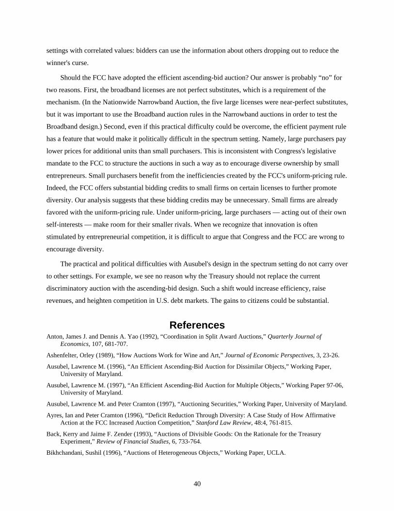
40
settings with correlated values: bidders can use the information about others dropping out to reduce the
winner's curse.
Should the FCC have adopted the efficient ascending-bid auction? Our answer is probably “no” for
two reasons. First, the broadband licenses are not perfect substitutes, which is a requirement of the
mechanism. (In the Nationwide Narrowband Auction, the five large licenses were near-perfect substitutes,
but it was important to use the Broadband auction rules in the Narrowband auctions in order to test the
Broadband design.) Second, even if this practical difficulty could be overcome, the efficient payment rule
has a feature that would make it politically difficult in the spectrum setting. Namely, large purchasers pay
lower prices for additional units than small purchasers. This is inconsistent with Congress's legislative
mandate to the FCC to structure the auctions in such a way as to encourage diverse ownership by small
entrepreneurs. Small purchasers benefit from the inefficiencies created by the FCC's uniform-pricing rule.
Indeed, the FCC offers substantial bidding credits to small firms on certain licenses to further promote
diversity. Our analysis suggests that these bidding credits may be unnecessary. Small firms are already
favored with the uniform-pricing rule. Under uniform-pricing, large purchasers — acting out of their own
self-interests — make room for their smaller rivals. When we recognize that innovation is often
stimulated by entrepreneurial competition, it is difficult to argue that Congress and the FCC are wrong to
encourage diversity.
The practical and political difficulties with Ausubel's design in the spectrum setting do not carry over
to other settings. For example, we see no reason why the Treasury should not replace the current
discriminatory auction with the ascending-bid design. Such a shift would increase efficiency, raise
revenues, and heighten competition in U.S. debt markets. The gains to citizens could be substantial.
ReferencesAnton, James J. and Dennis A. Yao (1992), “Coordination in Split Award Auctions,” Quarterly Journal of
Economics, 107, 681-707.
Ashenfelter, Orley (1989), “How Auctions Work for Wine and Art,” Journal of Economic Perspectives, 3, 23-26.
Ausubel, Lawrence M. (1996), “An Efficient Ascending-Bid Auction for Dissimilar Objects,” Working Paper,University of Maryland.
Ausubel, Lawrence M. (1997), “An Efficient Ascending-Bid Auction for Multiple Objects,” Working Paper 97-06,University of Maryland.
Ausubel, Lawrence M. and Peter Cramton (1997), “Auctioning Securities,” Working Paper, University of Maryland.
Ayres, Ian and Peter Cramton (1996), “Deficit Reduction Through Diversity: A Case Study of How AffirmativeAction at the FCC Increased Auction Competition,” Stanford Law Review, 48:4, 761-815.
Back, Kerry and Jaime F. Zender (1993), “Auctions of Divisible Goods: On the Rationale for the TreasuryExperiment,” Review of Financial Studies, 6, 733-764.
Bikhchandani, Sushil (1996), “Auctions of Heterogeneous Objects,” Working Paper, UCLA.
41
Bikhchandani, Sushil and John W. Mamer (1997), “Competitive Equilibrium in an Exchange Economy withIndivisibilities,” Journal of Economic Theory, 74, 385-413.
Bolle, Friedel (1995), “Necessary Conditions for Efficient Multiple-Bid Auctions,” Working Paper, Europa-Universitat Viadrina.
Bulow, Jeremy and Paul Klemperer (1996), “Auctions vs. Negotiations,” American Economic Review, 86, 180-194.
Chari, V. V. and Robert J. Weber (1992), “How the U.S. Treasury Should Auction Its Debt,” Quarterly Review,Federal Reserve Bank of Minneapolis, 3-12.
Coase, Ronald H. (1972), “Durability and Monopoly,” Journal of Law and Economics, 15, 143-149.
Cramton, Peter (1995), “Money Out of Thin Air: The Nationwide Narrowband PCS Auction,” Journal of Economicsand Management Strategy, 4, 267-343.
Cramton, Peter (1997), “The FCC Spectrum Auctions: An Early Assessment,” Journal of Economics andManagement Strategy, 6:3, 431-495.
Engelbrecht-Wiggans, Richard (1988), “Revenue Equivalence in Multi-object Auctions,” Economic Letters, 26, 15-19.
Engelbrecht-Wiggans, Richard and Charles M. Kahn (1995a), “Multi-Unit Auctions with Uniform Prices,” WorkingPaper, University of Illinois.
Friedman, Milton (1960), A Program for Monetary Stability, New York, NY: Fordham University Press.
Gul, Faruk and Ennio Stacchetti (1997a), “English Auctions with Multiple Goods,” Working Paper, PrincetonUniversity.
Gul, Faruk and Ennio Stacchetti (1997b), “Walrasian Equilibrium without Consumption Complementarities,”Working Paper, Princeton University.
Harris, Milton and Arthur Raviv (1981), “Allocation Mechanisms and the Design of Auctions,” Econometrica, 49,1477-1499.
Harstad, Ronald M. (1990), “Alternative Common-Value Auction Procedures: Revenue Comparisons with FreeEntry,” Journal of Political Economy, 98, 421-429.
Harstad, Ronald M. (1993), “Auctions with Endogenous Bidder Participation,” Working Paper, Rutgers University.
Katzman, Brett Eric (1995), “Multi-Unit Auctions with Incomplete Information,” Working Paper, Duke University.
Kelso, Alexander S. and Vincent P. Crawford (1982), “Job Matching, Coalition Formation, and Gross Substitutes,”Econometrica, 50, 1483-1504.
Levin, Dan and James L. Smith (1994), “Equilibrium in Auctions with Entry,” American Economic Review, 84, 585-599.
Levin, Dan and James L. Smith (1995), “Auctions with Entry: An Experimental Investigation,” Working Paper,Ohio State University.
Levin, Dan and James L. Smith (1996), “Optimal Reservation Prices in Auctions,” Economic Journal, 106,forthcoming.
Luenberger, David G. (1969), Optimization by Vector Space Methods, New York: John Wiley and Sons.
Malvey, Paul F., Christine M. Archibald, and Sean T. Flynn (1996), “Uniform-Price Auctions: Evaluation of theTreasury Experience,” Working Paper, U.S. Treasury.
Maskin, Eric S. and John G. Riley (1989), “Optimal Multi-unit Auctions,” in Frank Hahn (ed) The Economics ofMissing Markets, Information, and Games, Oxford: Oxford University Press, 312-35.
Maxwell, Christopher (1983), “Auctioning Divisible Commodities: A Study of Price Determination,” DoctoralDissertation, Harvard University.
42
McAfee, R. Preston and John McMillan (1987), “Auctions and Bidding,” Journal of Economic Literature, 25, 699-738.
McAfee, R. Preston and John McMillan (1996), “Analyzing the Airwaves Auction,” Journal of EconomicPerspectives, 10, 159-176.
McMillan, John (1994), “Selling Spectrum Rights,” Journal of Economic Perspectives, 8, 145-162.
Milgrom, Paul (1998), Putting Auctions to Work, forthcoming, Cambridge, England: Cambridge University Press.
Milgrom, Paul and Robert J. Weber (1982), “A Theory of Auctions and Competitive Bidding,” Econometrica, 50,1089-1122.
Myerson, Roger B. (1981), “Optimal Auction Design,” Mathematics of Operations Research, 6, 58-73.
Noussair, Charles (1995), “Equilibria in a Multi-Object Uniform Price Sealed Bid Auction with Multi-UnitDemands,” Economic Theory, 5, 337-351.
Reinhart, Vincent and Gregory Belzer (1996), “Some Evidence on Bid Shading and the Use of Information in theU.S. Treasury's Auction Experiment,” Working Paper, Board of Governors of the Federal Reserve System.
Riley, John G. and William F. Samuelson (1981), “Optimal Auctions,” American Economic Review, 71, 381-392.
Rothkopf, Michael H., Thomas J. Teisberg, and Edward P. Kahn (1990), “Why Are Vickrey Auctions Rare?”Journal of Political Economy, 98, 94-109.
Smith, Vernon L. (1967), “Experimental Studies of Discrimination versus Competition in Sealed-Bid AuctionMarkets,” Journal of Business, 40, 58-84.
Smith, Vernon L. (1982), “Microeconomic Systems as an Experimental Science,” American Economic Review, 72,923-955.
Tenorio, Rafael (1996), “On Strategic Quantity Bidding in Multiple Unit Auctions,” Working Paper, Notre DameUniversity.
Department of the Treasury, Securities and Exchange Commission, and Board of Governors of the Federal ReserveSystem (1992), Joint Report on the Government Securities Market, U.S. Government Printing Office, January.
Vickrey, William (1961), “Counterspeculation, Auctions, and Competitive Sealed Tenders,” Journal of Finance, 16,8-37.
Vickrey, William (1962), “Auction and Bidding Games,” in Recent Advances in Game Theory, Princeton UniversityConference, 15-29.
Wang, James J.D. and Jaime F. Zender (1996), “Auctioning Divisible Goods,” Working Paper, University of Utah.
Weber, Robert J. (1983), “Multiple-Object Auctions,” in Richard Engelbrecht-Wiggans, Martin Shubik, and RobertM. Stark (eds) Auctions, Bidding, and Contracting: Uses and Theory, New York: New York University Press,165-191.
Wilson, Robert (1979), “Auction of Shares,” Quarterly Journal of Economics, 94, 675-689.
Wolfram, Catherine D. (1996), “Strategic Bidding in a Multi-Unit Auction: An Empirical Analysis of Bids toSupply Electricity in England and Wales,” Working Paper, Harvard University.
Recommended