Review of Economics & Finance
Submitted on 07/June/2011
Article ID: 1923-7529-2011-05-01-16 Nikolaos Dritsakis
~ 1 ~
Demand for Money in Hungary: An ARDL Approach
Prof. Nikolaos Dritsakis
Department of Applied Informatics
University of Macedonia Economics and Social Sciences
156 Egnatia Street, 540 06 Thessaloniki, GREECE
E-mail: [email protected]
Abstract: This study examines the demand for money in Hungary using the autoregressive
distributed lag (ARDL) cointegration framework. The results based on the bounds testing procedure
confirm that a stable, long-run relationship exists between demand for money and its determinants:
real income, inflation rate and nominal exchange rate. The empirical results show that there is a
unique cointegrated and stable long-run relationship among M1 real monetary aggregate, real
income, inflation rate and nominal exchange rate. We find that the real income elasticity coefficient
is positive while the inflation rate elasticity and nominal exchange rate are negative. This indicates
that depreciation of domestic currency decreases the demand for money. Our results also reveal that
after incorporating the CUSUM and CUSUMSQ tests, M1 money demand function is stable
between 1995:1 and 2010:1.
JEL Classifications: E4, E41, E44
Keywords: Money demand, ARDL, Stability, Hungary
1. Introduction
The demand for money function creates a background to review the effectiveness of monetary
policies, as an important issue in terms of the overall macroeconomic stability. Money demand is an
important indicator of growth for a particular economy. The increasing money demand mostly
indicates a country's improved economic situation, as opposed to the falling demand which is
normally a sign of deteriorating economic climate (Maravić and Palić 2010). Monetarists underline
the role of governments in controlling for the amount of money in circulation. Their view on
monetary economics is that the variation on money supply has major influence on national product
in the short run and on price level in the long run. Also, they claim that the objectives of monetary
policy are best met by targeting the rate of increase on money supply.
Monetarism today is mainly associated with the work of Friedman, who was among the
generation of economists to accept Keynesian economics and then criticize it on its own terms.
Friedman argued that "inflation is always and everywhere a monetary phenomenon." Also, he
advocated a central bank policy aimed at keeping the supply and demand for money in equilibrium,
as measured by growth in productivity and demand. The European Central Bank officially bases its
monetary policy on money supply targets. Opponents of monetarism, including neo-Keynesians,
argue that demand for money is intrinsic to supply, while some conservative economists argue that
demand for money cannot be predicted. Stiglitz has claimed that the relationship between inflation
and money supply growth is weak when inflation is low (Friedman1970).
In 1980s, a number of central banks world-wide adopted monetary targets as a guide for
monetary policy. Central banks’ effort is to describe and determine the optimum money stock
which will produce (achieve) the desired macroeconomic objectives. Theoretically, central banks
ISSNs: 1923-7529; 1923-8401 © 2011 Academic Research Centre of Canada
~ 2 ~
had to aim between either the stock of monetary aggregates or interest rates. When money demand
function was unstable, interest rate was generally the preferred target. Otherwise, money stock was
the appropriate one (Poole 1970).
In 1990s, some central banks adopted numerical inflation or nominal GDP targets as guides for
monetary policy in contrast to the conventional choice of interest rate or money stock adopted in the
previous decade. Economic analysts attribute this change to the failure of monetary aggregates of
banks as guides for monetary policy. In addition, it is assumed that money demand function is
stable in the conduct and implementation of monetary policy. This is very important because money
demand function is used for the purpose of controlling the total liquidity in the economy and for
controlling inflation rate (Oluwole and Olugbenga 2007).
There are short-term and long-term aspects of money demand. The growing production relates
to the long-term aspect of money demand or the need for money (transaction demand). This means
that the increased issue of money which is consistent with price stability may solely be achieved in
the long run if it follows the growth of output. In the short term, a decreasing rate of money
circulation may cause the money demand to rise irrespective of the movements in real production.
However, the ongoing increase in money supply, regardless of the trends in production, leads to the
stronger inflatory pressures (Maravić and Palić 2010).
A stable relationship between money, a stock, and its determinants is a prerequisite for
monitoring and targeting of monetary aggregates. If a stable money demand function exists, the
central bank may rely on its monetary policy to affect important macroeconomic variables. Indeed,
the success of the policy depends on whether there exists a steady-state relationship between money
demand and its determinants (Baharumshah, et al. 2009).
After the collapse of former Soviet Union in the beginning of the 1990’s and with the
membership of the European Union, the Hungarian economy went through some significant
structural and institutional changes. These changes included the liberalization of the external trade,
the elimination of price and interest rate controls, the adoption of a managed float exchange rate
system as well as the changes in monetary policy including innovations in the banking sector. It is
conceivable that these developments have changed the relationship between money, income, prices
and other basic economic variables making money demand function structurally unstable.
Therefore, it is urgent to determine if the money demand function is stable throughout the examined
period.
A considerable body of literature has investigated the stability of money demand in developing
countries. The results and implications of these studies clearly depend on the data frequency, the
econometric methods for stability tests, and the development stage of a country. Several studies
have used ARDL cointegrating technique in examining the long run relationship between the
demand for money and its determinants. Some of these studies are: Halicioglu and Ugur (2005) for
Turkey, Bahmani-Oskooee and Rehman (2005) for seven Asian countries, Akinlo (2006) for
Nigeria, Samreth (2008) for Cambodia, Long and Samreth (2008) for Philippines, Baharumshah, et
al. (2009) for China, and Achsani, (2010) for Indonesia.
Halicioglu and Ugur (2005) analysed the stability of the narrow money demand function (M1)
in Turkey using annual data over the period 1950-2002. They estimated the test for stability of
Turkish M1 by employing a recent single cointegration procedure proposed by Pesaran et al. (2001)
along with the CUSUM and CUSUMSQ stability tests. They demonstrated that there is a stable
money demand function and it could be used as an intermediate target of monetary policy in
Turkey.
Bahmani-Oskooee and Rehman (2005) used quarterly data from 1973 to 2000 to estimate the
demand for money for seven Asian countries: India, Indonesia, Malaysia, Pakistan, Philippines,
Singapore and Thailand. Using ARDL approach and CUSUM and CUSUMSQ tests, they found
Review of Economics & Finance
~ 3 ~
that in some Asian countries even though real M1 or M2 monetary aggregates are cointegrated with
their determinants, the estimated parameters are unstable.
Akinlo (2006) used quarterly data over the period 1970:1–2002:4 and the ARDL approach
combined with CUSUM and CUSUMSQ tests, to examine the cointegrating property and stability
of M2 money demand for Nigeria. The results show M2 to be cointegrated with income, interest
rate and exchange rate. Moreover, the results revealed somewhat stable relation mainly with the
CUSUM test.
Samreth (2008) estimated the money demand function in Cambodia using monthly data over
the period 1994:12-2006:12. For the analysis of cointegration, the autoregressive distributed lag
(ARDL) approach is employed. Their results indicate that there is a cointegrating relationship
among variables (M1, Industrial Production Index, Consumer Price Index, and Nominal Exchange
Rate) in money demand function. CUSUM and CUSUMSQ tests roughly support the stability of
estimated model.
Long and Samreth (2008) re-examine the validity of both short and long run monetary models
of exchange rate for the case of Philippines by using ARDL approach. The results end up to robust
short and long run relationships between variables in the monetary exchange rate model of the
Philippines, as well as the stability of the estimated parameters.
Baharumshah, et al. (2009) examined the demand for broad money (M2) in China using the
autoregressive distributed lag (ARDL) cointegration framework and quarterly data from 1990:4 -
2007:2. The results based on the bounds testing procedure confirm that a stable, long-run
relationship exists between M2 and its determinants: real income, inflation, foreign interest rates
and stock prices.
Achsani (2010) used the vector error correction model (VECM) and autoregressive distributed
lag (ARDL) approach, and investigated the M2 money demand for Indonesia using quarterly data
over 1990:1-2008:3 period. He found that the ARDL model is more appropriate in predicting stable
money demand function of Indonesia in comparison to VECM.
Finally, Claudia Bush (2001) analyses the determinants and the stability of money demand
functions in Hungary and Poland using a restricted sample with monthly data for the years 1991
through mid-1998, and an error-correction model. The results of this paper suggest that long-run
parameters are in line with economic theory. However, on the basis of these findings alone would
be premature, the paper suggests that money demand functions can serve as a useful appropriateness
of different strategies for mapping the monetary policy of the examined countries.
Our paper differs from that of Bush in the following:
The size and the examined period for the money demand function.
The model that we implement in relation to that of Bush. (ARDL model is applied in all variables either they are integrated I(0) or integrated I(1).
Results of our paper suggest that money demand function M1 is the most suitable for Hungary for the period that we examine.
The general observation from the literature is that most studies, as far as the stability of the
demand for money function is concerned, have been focused mainly on advanced economies and
less on the industrialized economies.
Specifically in Hungary, (as far as we know) no study has used the autoregressive distributed
lag approach (ARDL) to examine the stability of the money demand function. So, there is the need
to fill this gap in the literature.
ISSNs: 1923-7529; 1923-8401 © 2011 Academic Research Centre of Canada
~ 4 ~
The purpose of this study is to examine whether the choice of Μ1 or M2 is the appropriate one
by examining the underlying assumption of the stability of money demand function for Hungary.
The aim of this paper is:
1) To investigate the empirical relationship between M1 and M2 real monetary aggregates, real income, inflation and nominal exchange rate using the autoregressive distributed lag (ARDL) cointegration model.
2) To determine the stability of M1 and M2 money demand function investigated.
This is important because as it has been proved, cointegration analysis cannot determine if there is a stable relationship of variables that we examine.
3) To investigate the long-run stability of the real money demand function based on the fact that the stability of the money demand function has important implications for the conduct and implementation of monetary policy.
The organization of the rest of this paper is as follows: on section 2 we introduce the model
and the ARDL approach. Section 3 presents the empirical results. Section 4 presents the
conclusions.
2. ARDL Approach
The autoregressive distributed lag (ARDL) model deals with single cointegration and is
introduced originally by Pesaran and Shin (1999) and further extended by Pesaran et al. (2001). The
ARDL approach has the advantage that it does not require all variables to be I(1) as the Johansen
framework and it is still applicable if we have I(0) and I(1) variables in our set.
The bounds test method cointegration has certain econometric advantages in comparison to
other methods of cointegration which are the following:
All variables of the model are assumed to be endogenous.
Bounds test method for cointegration is being applied irrespectively the order of integration of the variable. There may be either integrated first order Ι(1) or Ι(0).
The short-run and long-run coefficients of the model are estimated simultaneously.
The overriding objective of monetary policy for every developing country is price and
exchange rate stability. The monetary authority’s strategy for inflation management is based on the
view that inflation is essentially a monetary phenomenon. Because targeting money supply growth
is considered as an appropriate method of targeting inflation, many central banks choose a monetary
targeting policy framework to achieve the objective of price stability (Oluwole and Olugbenga,
2007).
From the policy standpoint, it is important to identify the correct measure of money as a better
path to monetary policy in order to achieve price stability. For this reason we take into
consideration both M1 and M2. Secondly, since the policy maker may be interested not only in the
forecasting power of such estimations but also in short-run relevance of the parameters, we use
quarterly data covering the period 1995:1 and 2010:1.
Following Bahmani-Oskooee (1996) and Bahmani-Oskooee and Rehman (2005) the model
includes real monetary aggregate, real income, inflation rate, and exchange rate, which can be
written in a semi-log linear form as:
LMt = a0 + a1LYt + a2INFt + a3LEXRt + ut (1)
Where, M is the real monetary aggregate (M1 or M2);
Review of Economics & Finance
~ 5 ~
Y is a measure of real income (at constant factor cost 2005 prices), with expected positive
elasticity;
INF is rate of inflation (base year 2005), with expected negative elasticity;
EXR is nominal effective exchange rate (forint, per US dollar), with expected positive or
negative elasticity, and u is error term.
LM=lnM, LY=lnY, LEXR=lnEXR. (All variables, except the rate of inflation are in natural logs).
According to Arango and Nadiri (1981) and Bahmani-Oskooee and Pourheydarian (1990),
while an estimate of α1 is expected to be positive, an estimate of α2 is expected to be negative.
Estimation of α3 could be negative or positive. Given that, EXR is defined as number of units of
domestic currency per US dollar, or ECU, a depreciation of the domestic currency or increase in
EXR raises the value of the foreign assets in terms of domestic currency. If this increase is caused
as an increase in wealth, then the demand for domestic money increases yielding a positive estimate
of α3. However, if an increase in EXR induces an expectation of further depreciation of the
domestic currency, public may hold less of domestic currency and more of foreign currency. In this
case, an estimate of α3 is expected to be negative (Sharifi-Renani 2007). An ARDL representation
of equation (1) is formulated as follows:
n
i
n
i
n
i
n
i
itiitiitiitit LEXPINFLYLMLM1 0 0 0
43210
ttttt eLEXPINFLYLM 14131211 (2)
where Γ denotes the first difference operator; α0 is the drift component, and et is the usual white
noise residuals.
The left-hand side is the demand for money. The first until fourth expressions (β1 –β4) on the
right-hand side correspond to the long-run relationship. The remaining expressions with the
summation sign (α1 – α4) represent the short-run dynamics of the model.
To investigate the presence of long-run relationships among the LM, LY, INF, LEXP, bound
testing under Pesaran, et al. (2001) procedure is used. The bound testing procedure is based on the
F-test. The F-test is actually a test of the hypothesis of no coinetegration among the variables
against the existence or presence of cointegration among the variables, denoted as:
Ho: β1 = β2 = β3 = β4 = 0, i.e., there is no cointegration among the variables.
Ha : β1 ≠ β2 ≠ β3 ≠ β4 ≠ 0, i.e., there is cointegration among these variables.
This can also be denoted: FLΜ(LΜ│LΥ, INF, LEXP).
The ARDL bound test is based on the Wald-test (F-statistic). The asymptotic distribution of the
Wald-test is non-standard under the null hypothesis of no cointegration among the variables. Two
critical values are given by Pesaran et al. (2001) for the cointegration test. The lower critical bound
assumes all the variables are I(0) meaning that there is no cointegration relationship between the
examined variables. The upper bound assumes that all the variables are I(1) meaning that there is
cointegration among the variables. When the computed F-statistic is greater than the upper bound
critical value, then the H0 is rejected (the variables are cointegrated). If the F-statistic is below the
lower bound critical value, then the H0 cannot be rejected (there is no cointegration among the
variables). When the computed F-statistics falls between the lower and upper bound, then the results
are inconclusive.
In the meantime, we develop the unrestricted error correction model (UECM) based on the
assumption made by Pesaran et al.(2001). From the unrestricted error correction model, the long-
ISSNs: 1923-7529; 1923-8401 © 2011 Academic Research Centre of Canada
~ 6 ~
run elasticities are the coefficient of the one lagged explanatory variable (multiplied with a negative
sign) divided by the coefficient of the one lagged dependent variable.
The ARDL has been chosen since it can be applied for a small sample size as it happens in this
study. Also, it can estimate the short and long-run dynamic relationships in demand of money
simultaneously. The ARDL methodology is relieved of the burden of establishing the order of
integration amongst the variables. Furthermore, it can distinguish dependent and explanatory
variables, and allows testing for the existence of relationship between the variables. Finally, with
the ARDL it is possible that different variables have differing optimal number of lags.
Thus, equation (2) in the ARDL version of the error correction model can be expressed as
equation (3): The error correction version of ARDL model pertaining to the variables in equation
(2) is as follows:
tt
n
i
n
i
n
i
n
i
itiitiitiitit uECLEXPINFLYLMLM
1
1 0 0 0
43210 (3)
where λ is the speed of adjustment parameter and EC is the residuals that are obtained from the
estimated cointegration model of equation (2).
3. Empirical Results
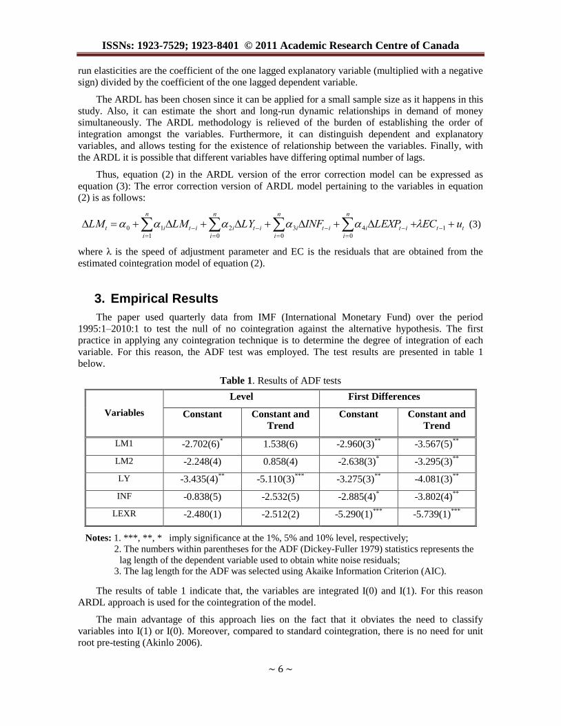
The paper used quarterly data from IMF (International Monetary Fund) over the period
1995:1–2010:1 to test the null of no cointegration against the alternative hypothesis. The first
practice in applying any cointegration technique is to determine the degree of integration of each
variable. For this reason, the ADF test was employed. The test results are presented in table 1
below.
Table 1. Results of ADF tests
Variables
Level First Differences
Constant Constant and
Trend
Constant Constant and
Trend
LM1 -2.702(6)* 1.538(6) -2.960(3)
** -3.567(5)
**
LM2 -2.248(4) 0.858(4) -2.638(3)* -3.295(3)
**
LY -3.435(4)**
-5.110(3)***
-3.275(3)**
-4.081(3)**
INF -0.838(5) -2.532(5) -2.885(4)* -3.802(4)
**
LEXR -2.480(1) -2.512(2) -5.290(1)***
-5.739(1)***
Notes: 1. ***, **, * imply significance at the 1%, 5% and 10% level, respectively;
2. The numbers within parentheses for the ADF (Dickey-Fuller 1979) statistics represents the
lag length of the dependent variable used to obtain white noise residuals;
3. The lag length for the ADF was selected using Akaike Information Criterion (AIC).
The results of table 1 indicate that, the variables are integrated I(0) and I(1). For this reason
ARDL approach is used for the cointegration of the model.
The main advantage of this approach lies on the fact that it obviates the need to classify
variables into I(1) or I(0). Moreover, compared to standard cointegration, there is no need for unit
root pre-testing (Akinlo 2006).
Review of Economics & Finance
~ 7 ~
The ARDL cointegration test, assumed that only one long run relationship exists between the
dependent variable and the exogenous variables (Pesaran, Shin and Smith, 2001, assumption 3). To
test whether this is really appropriate in the current application, we change the entire variable to be
dependent variable in order to compute the F-statistic for the respective joint significance in the
ARDL models (Ahmad Abd Halim et al. 2008).
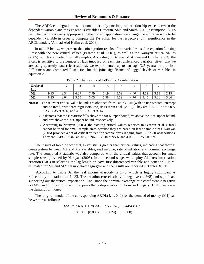
In table 2 below, we present the cointegration results of the variables used in equation 2, using
F-test with the new critical values (Pesaran et al. 2001), as well as the Narayan critical values
(2005), which are quoted in small samples. According to Bahmani-Oskooee and Brooks (2003), the
F-test is sensitive to the number of lags imposed on each first differenced variable. Given that we
are using quarterly data (observations), we experimented up to ten lags (2.5 years) on the first-
differences and computed F-statistics for the joint significance of lagged levels of variables in
equation 2.
Table 2. The Results of F-Test for Cointegration
Order of Lag
1 2 3 4 5 6 7 8 9 10
M1 9.93***
8.34***
6.87***
7.79***
6.19***
5.62***
4.40**
4.12* 3.13 2.15
M2 8.15***
8.04***
5.55**
6.05***
5.58**
5.52**
4.76**
5.45**
5.06**
3.86*
Notes: 1.The relevant critical value bounds are obtained from Table C1.iii (with an unrestricted intercept
and no trend; with three regressors k=3) in Pesaran et al. (2001). They are 2.72 - 3.77 at 90%,
3.23 - 4.35 at 95%, and 4.29 – 5.61 at 99%;
2. * denotes that the F-statistic falls above the 90% upper bound, ** above the 95% upper bound,
and *** above the 99% upper bound, respectively;
3. According to Narayan (2005), the existing critical values reported in Pesaran et al. (2001)
cannot be used for small sample sizes because they are based on large sample sizes. Narayan
(2005) provides a set of critical values for sample sizes ranging from 30 to 80 observations.
They are 2.496 - 3.346 at 90%, 2.962 – 3.910 at 95%, and 4.068 – 5.250 at 99%.
The results of table 2 show that, F-statistic is greater than critical values, indicating that there is
cointegration between M1 and M2 variables, real income, rate of inflation and nominal exchange
rate. The computed F-statistic was also compared with the critical values that account for small
sample sizes provided by Narayan (2005). In the second stage, we employ Akaike's information
criterion (AIC) in selecting the lag length on each first differenced variable and equation 2 is re-
estimated for M1 and M2 real monetary aggregate and the results are reported in Tables 3a, 3b.
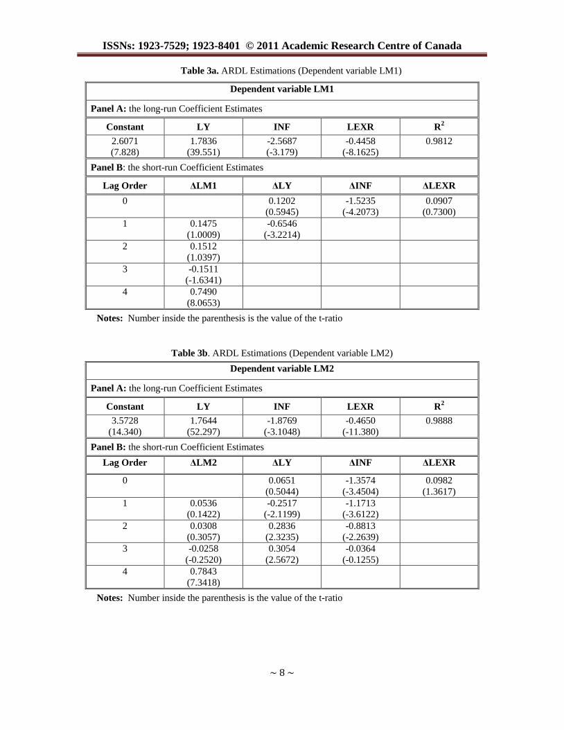
According to Table 3a, the real income elasticity is 1.78, which is highly significant as
reflected by a t-statistic of 10.83. The inflation rate elasticity is negative (-2.568) and significant
supporting our theoretical expectation. And, since the nominal exchange rate coefficient is negative
(-0.445) and highly significant, it appears that a depreciation of forint in Hungary (HUF) decreases
the demand for money.
The long-run model of the corresponding ARDL(4, 1, 0, 0) for the demand of money (M1) can
be written as follows:
LM1t = 2.607 + 1.783LYt – 2.568INFt – 0.445LEXRt
(0.000) (0.000) (0.0024) (0.000)
ISSNs: 1923-7529; 1923-8401 © 2011 Academic Research Centre of Canada
~ 8 ~
Table 3a. ARDL Estimations (Dependent variable LM1)
Dependent variable LM1
Panel A: the long-run Coefficient Estimates
Constant LY INF LEXR R2
2.6071
(7.828)
1.7836
(39.551)
-2.5687
(-3.179)
-0.4458
(-8.1625)
0.9812
Panel B: the short-run Coefficient Estimates
Lag Order ΔLM1 ΔLY ΔINF ΔLEXR
0 0.1202
(0.5945)
-1.5235
(-4.2073)
0.0907
(0.7300)
1 0.1475
(1.0009)
-0.6546
(-3.2214)
2 0.1512
(1.0397)
3 -0.1511
(-1.6341)
4 0.7490
(8.0653)
Notes: Number inside the parenthesis is the value of the t-ratio
Table 3b. ARDL Estimations (Dependent variable LM2)
Dependent variable LM2
Panel A: the long-run Coefficient Estimates
Constant LY INF LEXR R2
3.5728
(14.340)
1.7644
(52.297)
-1.8769
(-3.1048)
-0.4650
(-11.380)
0.9888
Panel B: the short-run Coefficient Estimates
Lag Order ΔLM2 ΔLY ΔINF ΔLEXR
0 0.0651
(0.5044)
-1.3574
(-3.4504)
0.0982
(1.3617)
1 0.0536
(0.1422)
-0.2517
(-2.1199)
-1.1713
(-3.6122)
2 0.0308
(0.3057)
0.2836
(2.3235)
-0.8813
(-2.2639)
3 -0.0258
(-0.2520)
0.3054
(2.5672)
-0.0364
(-0.1255)
4 0.7843
(7.3418)
Notes: Number inside the parenthesis is the value of the t-ratio
Review of Economics & Finance
~ 9 ~
According to Table 3b, the real income elasticity is 1.76, which is highly significant as
reflected by a t-statistic of 52.29. The inflation rate elasticity is negative (-1.876) and significant
supporting our theoretical expectation. And, since the nominal exchange rate coefficient is negative
(-0.465) and highly significant, it appears that a depreciation of forint in Hungary (HUF) decreases
the demand for money.
The long-run model of the corresponding ARDL(4, 3, 3, 0) for the demand for money (M2) can
be written as follows:
LM2t = 3.572 + 1.764LYt – 1.876INFt – 0.465LEXRt
(0.000) (0.000) (0.003) (0.000)
High coefficients of long run income elasticity turn to be opposite with the hypothesis of
economies of scale in money holding predicted by the transactions. This can be interpreted mainly
in the case where we use a broader definition of money M2 which includes some advantages such
as time deposits and savings. It is important to point out that when income elasticity is larger than
one, an outstanding matter appears in the literature both for developed and developing countries.
Inflation is negatively correlated to real demand for money, meaning that the higher the inflation
rate the lower is the demand for money. The coefficient of the expecting exchange rate is negative
and at the same time statistical significant both for M1 and M2. The statistically significant negative
coefficient of the expected exchange rate indicates the existence of the currency substitution in
Hungary.
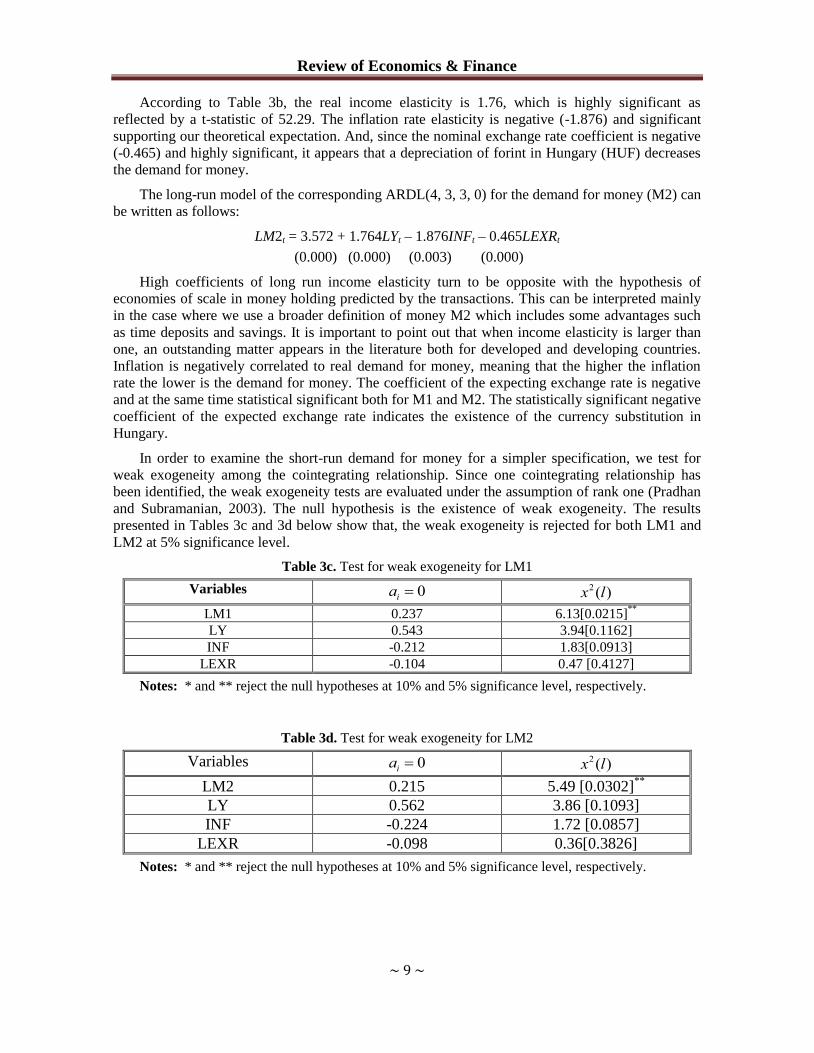
In order to examine the short-run demand for money for a simpler specification, we test for
weak exogeneity among the cointegrating relationship. Since one cointegrating relationship has
been identified, the weak exogeneity tests are evaluated under the assumption of rank one (Pradhan
and Subramanian, 2003). The null hypothesis is the existence of weak exogeneity. The results
presented in Tables 3c and 3d below show that, the weak exogeneity is rejected for both LM1 and
LM2 at 5% significance level.
Table 3c. Test for weak exogeneity for LM1
Variables 0ia )(2 lx
LM1 0.237 6.13[0.0215]**
LY 0.543 3.94[0.1162]
INF -0.212 1.83[0.0913]
LEXR -0.104 0.47 [0.4127]
Notes: * and ** reject the null hypotheses at 10% and 5% significance level, respectively.
Table 3d. Test for weak exogeneity for LM2
Variables 0ia )(2 lx
LM2 0.215 5.49 [0.0302]**
LY 0.562 3.86 [0.1093]
INF -0.224 1.72 [0.0857]
LEXR -0.098 0.36[0.3826]
Notes: * and ** reject the null hypotheses at 10% and 5% significance level, respectively.
ISSNs: 1923-7529; 1923-8401 © 2011 Academic Research Centre of Canada
~ 10 ~
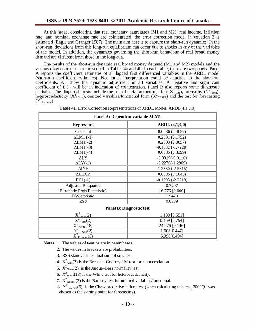
At this stage, considering that real monetary aggregates (M1 and M2), real income, inflation rate, and nominal exchange rate are cointegrated, the error correction model in equation 2 is estimated (Engle and Granger 1987). The main aim here is to capture the short-run dynamics. In the short-run, deviations from this long-run equilibrium can occur due to shocks in any of the variables of the model. In addition, the dynamics governing the short-run behaviour of real broad money demand are different from those in the long-run.
The results of the short-run dynamic real broad money demand (M1 and M2) models and the various diagnostic tests are presented in Tables 4a and 4b. In each table, there are two panels. Panel A reports the coefficient estimates of all lagged first differenced variables in the ARDL model (short-run coefficient estimates). Not much interpretation could be attached to the short-run coefficients. All show the dynamic adjustment of all variables. A negative and significant coefficient of ECt-1 will be an indication of cointegration. Panel B also reports some diagnostic statistics. The diagnostic tests include the test of serial autocorrelation (X
2Auto), normality (X
2Norm),
heteroscedasticity (X2
White), omitted variables/functional form (X2
RESET) and the test for forecasting (X
2Forecast).
Table 4a. Error Correction Representations of ARDL Model, ARDL(4,1,0,0)
Panel A: Dependent variable ΔLM1
Regressors ARDL (4,1,0,0)
Constant 0.0036 (0.4057)
ΓLM1 (-1)
ΓLM1(-2)
ΓLM1(-3)
ΓLM1(-4)
0.2331 (2.1752)
0.2003 (2.0057)
-0.1882 (-1.7228)
0.6385 (6.3399)
ΓLY
ΓLY(-1)
-0.0019(-0.0110)
-0.2270(-1.2909)
ΓINF -1.2330 (-2.5815)
ΓLEXR 0.0085 (0.1045)
EC1(-1) -0.1295 (-2.2219)
Adjusted R-squared 0.7207
F-statistic Prob(F-statistic) 16.776 [0.000]
DW-statistic 1.9470
RSS 0.0389
Panel B: Diagnostic test
X2Auto(2) 1.189 [0.551]
X2
Norm(2) 0.459 [0.794]
X2
White(18) 24.276 [0.146]
X2
RESET(2) 1.608[0.447]
X2
Forecast(5) 5.090[0.404]
Notes: 1. The values of t-ratios are in parentheses.
2. The values in brackets are probabilities.
3. RSS stands for residual sum of squares.
4. X2
Auto(2) is the Breusch–Godfrey LM test for autocorrelation.
5. X2
Norm(2) is the Jarque–Bera normality test.
6. X2
White(18) is the White test for heteroscedasticity.
7. X2
RESET(2) is the Ramsey test for omitted variables/functional.
8. X2Forecast(5) is the Chow predictive failure test (when calculating this test, 2009Q1 was
chosen as the starting point for forecasting).
Review of Economics & Finance
~ 11 ~
As can be seen from Table 4a at panel Α, the ECt-1 carries an expected negative sign, which is
highly significant, indicating that, M1, real income, inflation rate, and nominal exchange rate are
cointegrated. The absolute value of the coefficient of the error-correction term indicates that about
13 percent of the disequilibrium in the real M1 demand is offset by short-run adjustment in each
quarterly. This means that excess money is followed in the next period by a reduction in the level of
money balances, which people would desire to hold. Thus, it is important to reduce the existing
disequilibrium over time in order to maintain long-run equilibrium.
The diagnostic tests presented in the lower panel Β of Table 4a show that there is no evidence
of diagnostic problem with the model. Measuring the explanatory power of the equations by their
adjusted R-squared shows that, roughly 72% of the variation in money demand can be explained.
The Lagrange Multiplier (LM) test of autocorrelation suggests that the residuals are not serially
correlated. According to the Jarque-Bera (JB) test, the null hypothesis of normally distributed
residuals cannot be rejected. The White heteroscedasticity test suggests that the disturbance term in
the equation is homoskedastic. The Ramsey RESET test result shows that the calculated Χ2-value is
less than the critical value at the five percent level of significance. This is an indication that there is
no specification error. Finally, the Chow predictive failure test shows that the model may be used
for forecasting.
Table 4b. Error Correction Representations of ARDL Model, ARDL(4,3,3,0)
Panel A: Dependent variable ΔLM2
Regressors ARDL (4,3,3,0)
Constant 0.0074 (0.7327)
ΓLM2 (-1)
ΓLM2(-2)
ΓLM2(-3)
ΓLM2(-4)
-0.0207 (-0.1320)
0.2134 (1.3282)
-0.0743 (-0.4918)
0.4891 (3.0119)
ΓLY
ΓLY(-1)
ΓLY(-2)
ΓLY(-3)
-0.1151 (-0.8243)
-0.1047 (-0.8032)
0.1670 (1.2620)
0.0258 (0.1940)
ΓINF
ΓINF(-1)
ΓINF(-2)
ΓINF(-3)
-0.4602 (-1.1030)
-0.7770 (-1.7037)
-0.5155 (-1.1607)
-0.0831 (-0.1969)
ΓLEXR 0.0696 (1.2041)
EC2(-1) -0.0618 (-1.0423)
Adjusted R-squared 0.5994
F-statistic Prob(F-statistic) 6.8783 [0.000]
DW-statistic 1.8903
RSS 0.0169
Panel B: Diagnostic test
X2Auto(2) 0.361 [0.834]
X2
Norm(2) 2.057 [0.357]
X2
White(18) 29.380 [0.393]
X2
RESET(2) 0.494 [0.780]
X2
Forecast(5) 26.293 [0.000]
ISSNs: 1923-7529; 1923-8401 © 2011 Academic Research Centre of Canada
~ 12 ~
Notes: 1. The values of t-ratios are in parentheses.
2. The values in brackets are probabilities.
3. RSS stands for residual sum of squares.
4. X2
Auto(2) is the Breusch–Godfrey LM test for autocorrelation.
5. X2
Norm(2) is the Jarque–Bera normality test.
6. X2
White(18) is the White test for heteroscedasticity.
7. X2
RESET(2) is the Ramsey test for omitted variables/functional.
8. X2Forecast(5) is the Chow predictive failure test (when calculating this test, 2009Q1 was
chosen as the starting point for forecasting).
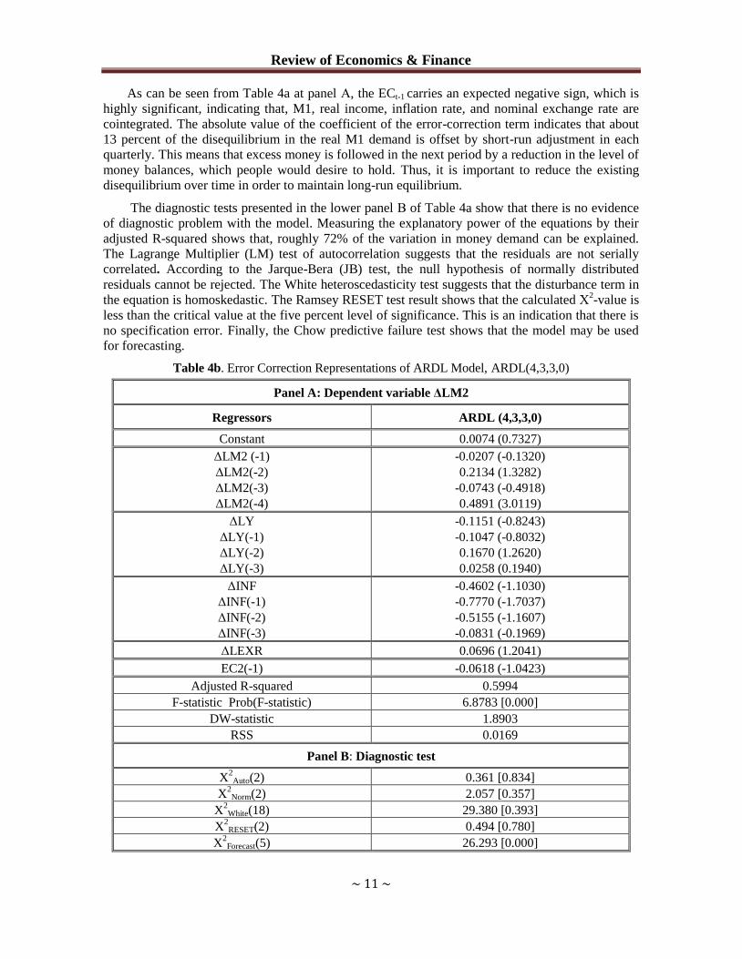
Table 4b reports the results for real M2 monetary aggregate. As can be seen, there is lack of
cointegration as indicated by the insignificant coefficient attached to ECt-1 or by insignificant long-
run coefficient estimates. Thus, it may be concluded that M1 is a better monetary aggregate in terms
of formulating monetary policy.
The existence of a stable and predictable relationship between the demand for money and its
determinants is considered a necessary condition for the formulation of monetary policy strategies
based on intermediate monetary targeting (Sharifi-Renani 2007). Τhe stability of the long-run
coefficients are used to form the error-correction term in conjunction with the short run dynamics.
Some of the problems of instability could stem from inadequate modelling of the short-run
dynamics characterizing departures from the long run relationship. Hence, it is expedient to
incorporate the short run dynamics for constancy of long run parameters. In view of this we apply
the CUSUM and CUSUMSQ tests, which Brown et al. (1975) developed.
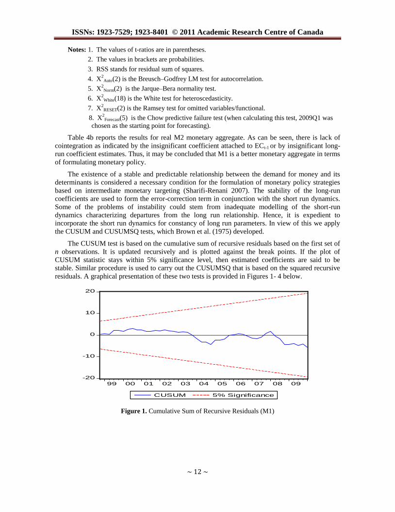
The CUSUM test is based on the cumulative sum of recursive residuals based on the first set of
n observations. It is updated recursively and is plotted against the break points. If the plot of
CUSUM statistic stays within 5% significance level, then estimated coefficients are said to be
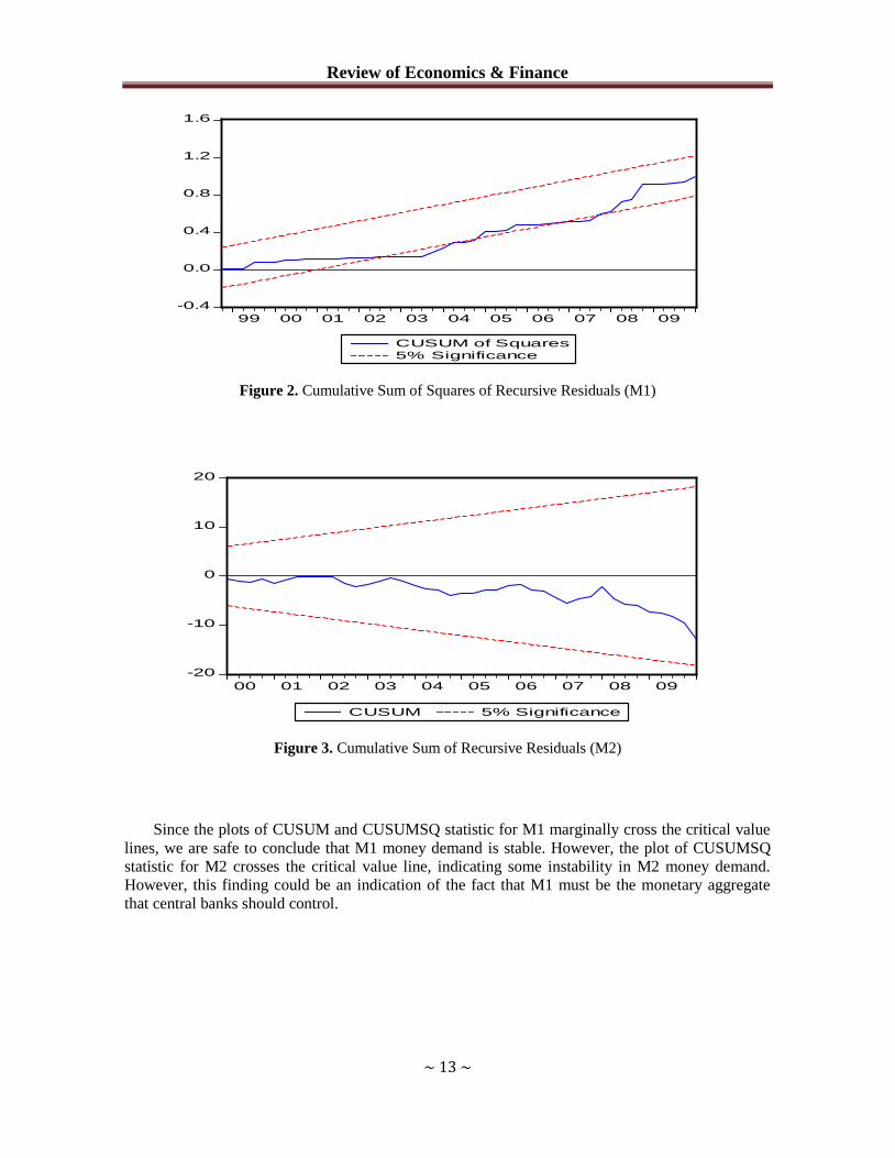
stable. Similar procedure is used to carry out the CUSUMSQ that is based on the squared recursive
residuals. A graphical presentation of these two tests is provided in Figures 1- 4 below.
Figure 1. Cumulative Sum of Recursive Residuals (M1)
-20
-10
0
10
20
99 00 01 02 03 04 05 06 07 08 09
CUSUM 5% Significance
Review of Economics & Finance
~ 13 ~
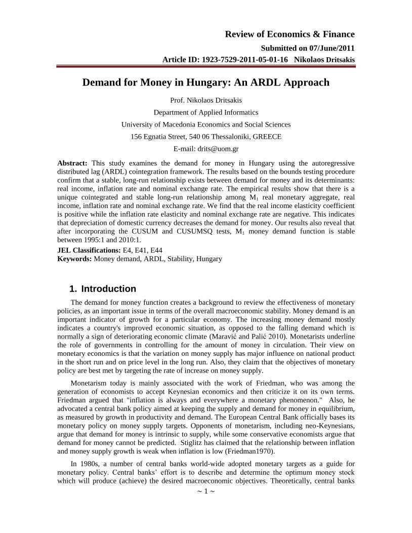
Figure 2. Cumulative Sum of Squares of Recursive Residuals (M1)
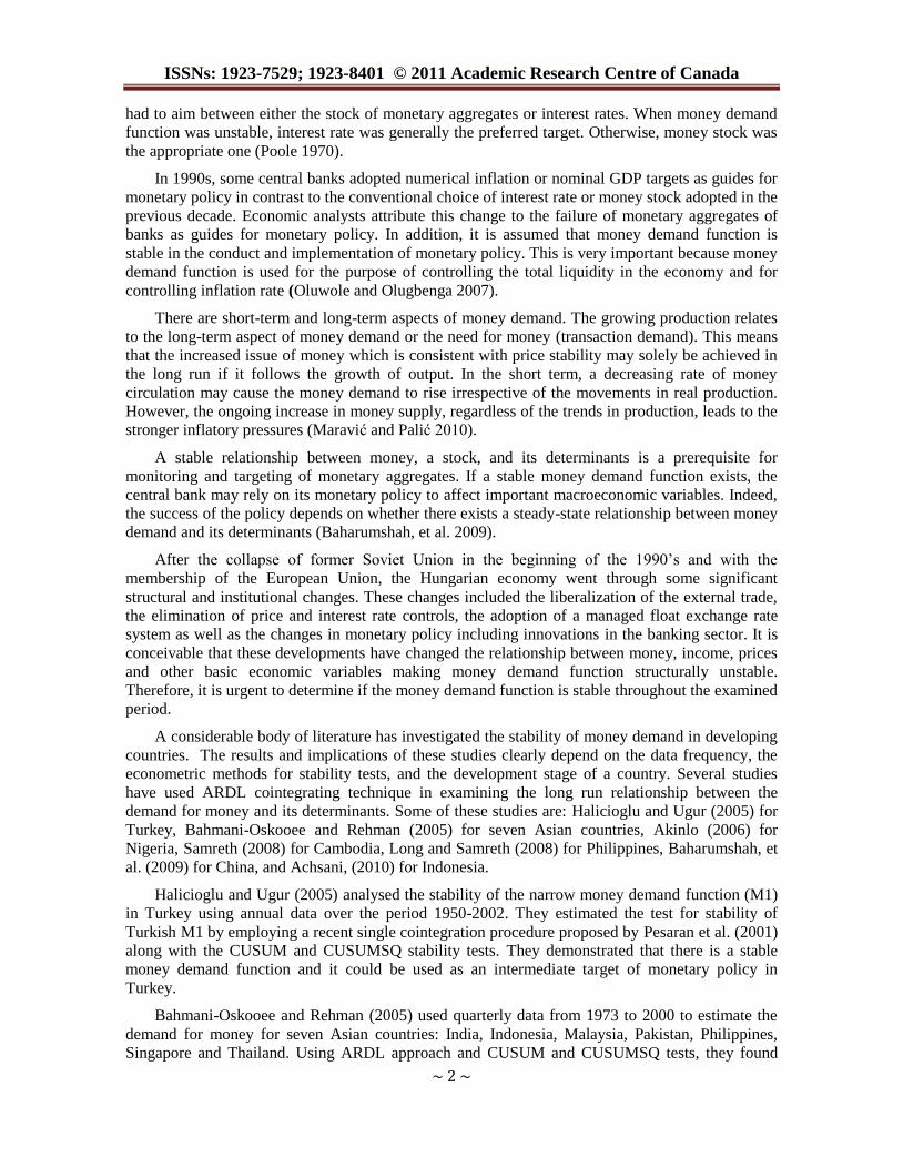
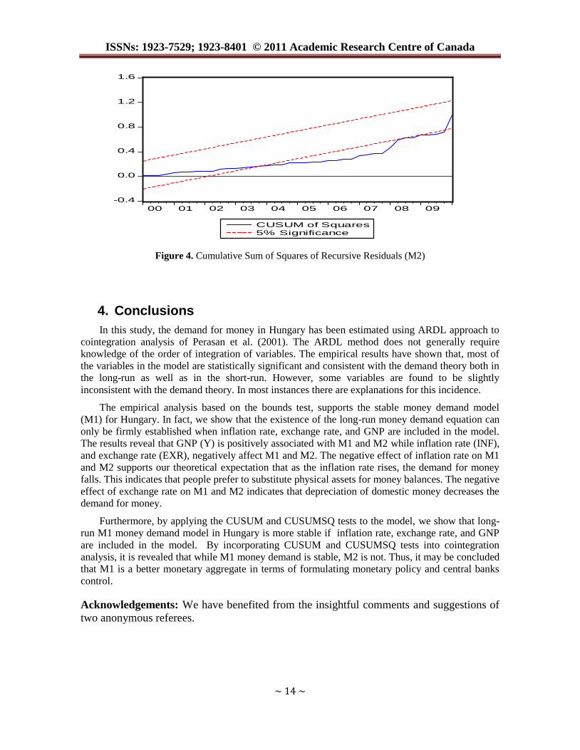
Figure 3. Cumulative Sum of Recursive Residuals (M2)
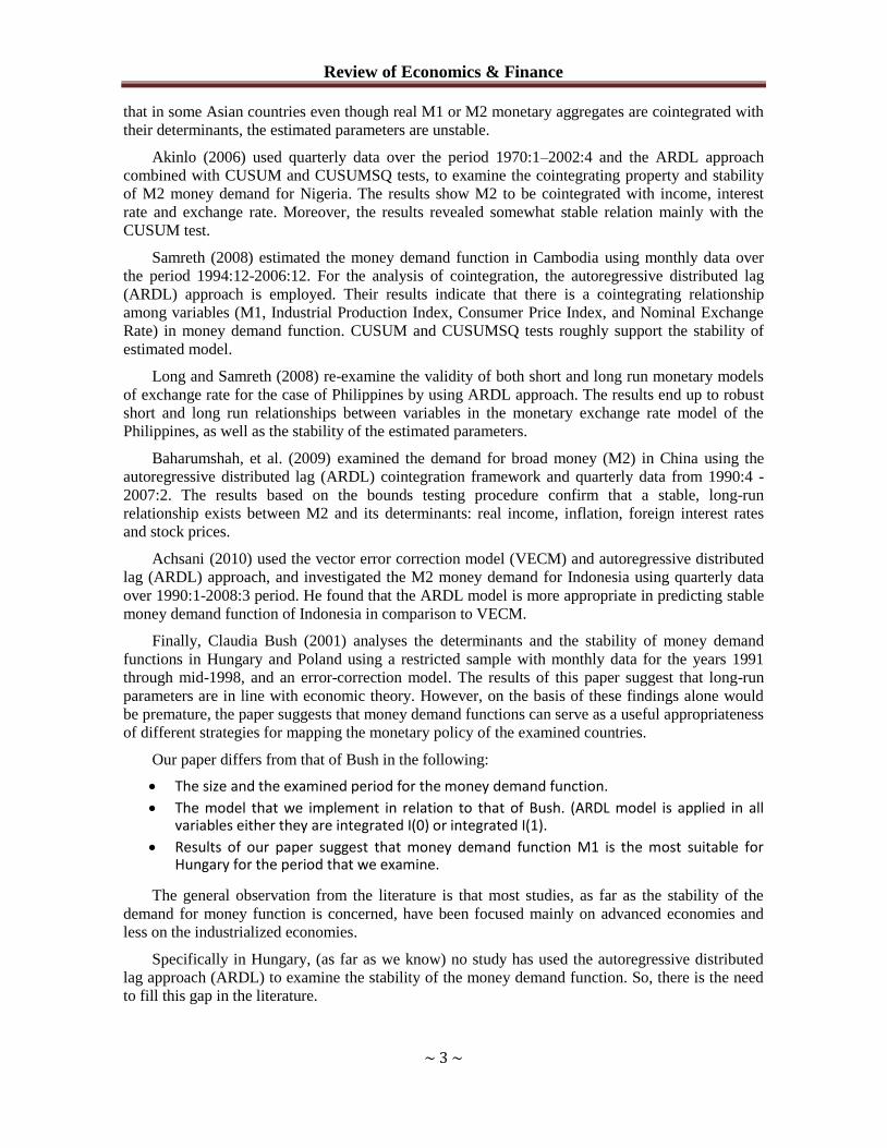
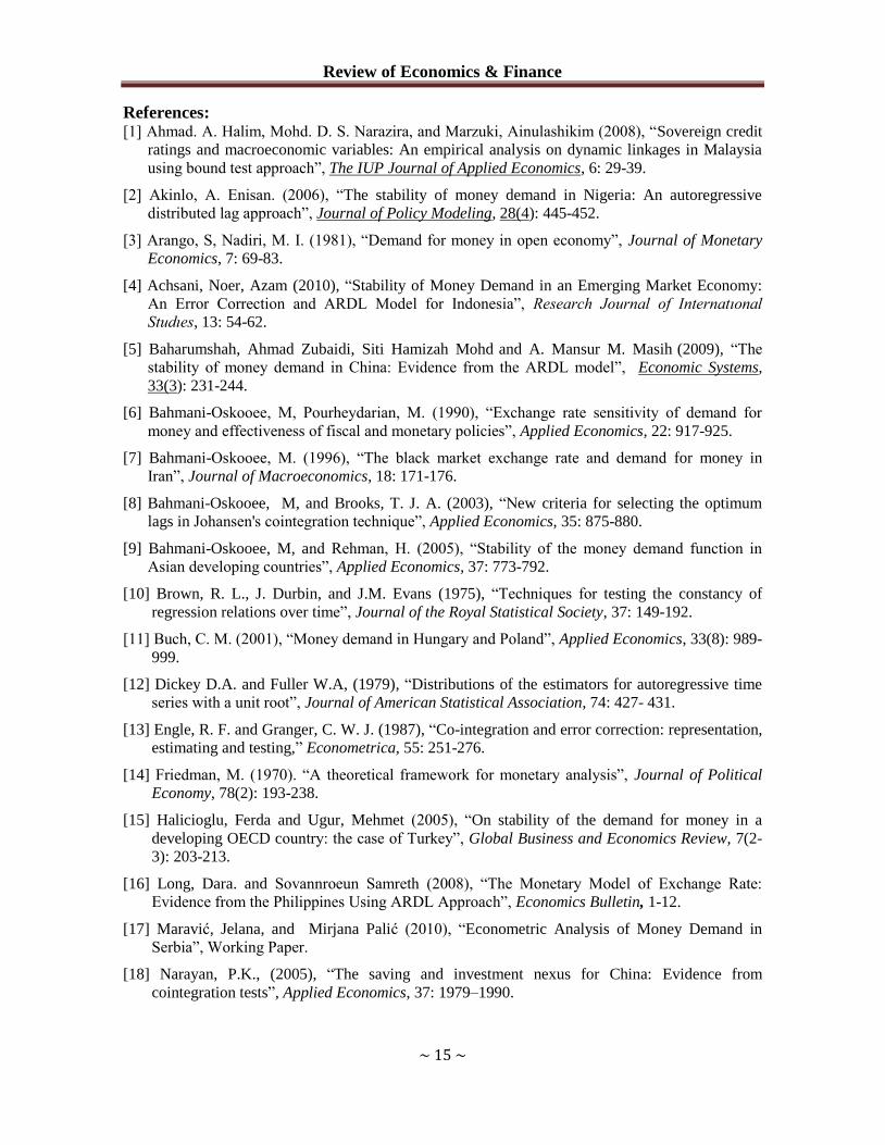
Since the plots of CUSUM and CUSUMSQ statistic for M1 marginally cross the critical value
lines, we are safe to conclude that M1 money demand is stable. However, the plot of CUSUMSQ
statistic for M2 crosses the critical value line, indicating some instability in M2 money demand.
However, this finding could be an indication of the fact that M1 must be the monetary aggregate
that central banks should control.
-0.4
0.0
0.4
0.8
1.2
1.6
99 00 01 02 03 04 05 06 07 08 09
CUSUM of Squares5% Significance
-20
-10
0
10
20
00 01 02 03 04 05 06 07 08 09
CUSUM 5% Significance
ISSNs: 1923-7529; 1923-8401 © 2011 Academic Research Centre of Canada
~ 14 ~
Figure 4. Cumulative Sum of Squares of Recursive Residuals (M2)
4. Conclusions
In this study, the demand for money in Hungary has been estimated using ARDL approach to
cointegration analysis of Perasan et al. (2001). The ARDL method does not generally require
knowledge of the order of integration of variables. The empirical results have shown that, most of
the variables in the model are statistically significant and consistent with the demand theory both in
the long-run as well as in the short-run. However, some variables are found to be slightly
inconsistent with the demand theory. In most instances there are explanations for this incidence.
The empirical analysis based on the bounds test, supports the stable money demand model
(M1) for Hungary. In fact, we show that the existence of the long-run money demand equation can
only be firmly established when inflation rate, exchange rate, and GNP are included in the model.
The results reveal that GNP (Y) is positively associated with M1 and M2 while inflation rate (INF),
and exchange rate (EXR), negatively affect M1 and M2. The negative effect of inflation rate on M1
and M2 supports our theoretical expectation that as the inflation rate rises, the demand for money
falls. This indicates that people prefer to substitute physical assets for money balances. The negative
effect of exchange rate on M1 and M2 indicates that depreciation of domestic money decreases the
demand for money.
Furthermore, by applying the CUSUM and CUSUMSQ tests to the model, we show that long-
run M1 money demand model in Hungary is more stable if inflation rate, exchange rate, and GNP
are included in the model. By incorporating CUSUM and CUSUMSQ tests into cointegration
analysis, it is revealed that while M1 money demand is stable, M2 is not. Thus, it may be concluded
that M1 is a better monetary aggregate in terms of formulating monetary policy and central banks
control.
Acknowledgements: We have benefited from the insightful comments and suggestions of
two anonymous referees.
-0.4
0.0
0.4
0.8
1.2
1.6
00 01 02 03 04 05 06 07 08 09
CUSUM of Squares5% Significance
Review of Economics & Finance
~ 15 ~
References: [1] Ahmad. A. Halim, Mohd. D. S. Narazira, and Marzuki, Ainulashikim (2008), “Sovereign credit
ratings and macroeconomic variables: An empirical analysis on dynamic linkages in Malaysia
using bound test approach”, The IUP Journal of Applied Economics, 6: 29-39.
[2] Akinlo, A. Enisan. (2006), “The stability of money demand in Nigeria: An autoregressive
distributed lag approach”, Journal of Policy Modeling, 28(4): 445-452.
[3] Arango, S, Nadiri, M. I. (1981), “Demand for money in open economy”, Journal of Monetary
Economics, 7: 69-83.
[4] Achsani, Noer, Azam (2010), “Stability of Money Demand in an Emerging Market Economy:
An Error Correction and ARDL Model for Indonesia”, Research Journal of Internatıonal
Studıes, 13: 54-62.
[5] Baharumshah, Ahmad Zubaidi, Siti Hamizah Mohd and A. Mansur M. Masih
(2009), “The
stability of money demand in China: Evidence from the ARDL model”, Economic Systems,
33(3): 231-244.
[6] Bahmani-Oskooee, M, Pourheydarian, M. (1990), “Exchange rate sensitivity of demand for
money and effectiveness of fiscal and monetary policies”, Applied Economics, 22: 917-925.
[7] Bahmani-Oskooee, M. (1996), “The black market exchange rate and demand for money in
Iran”, Journal of Macroeconomics, 18: 171-176.
[8] Bahmani-Oskooee, M, and Brooks, T. J. A. (2003), “New criteria for selecting the optimum
lags in Johansen's cointegration technique”, Applied Economics, 35: 875-880.
[9] Bahmani-Oskooee, M, and Rehman, H. (2005), “Stability of the money demand function in
Asian developing countries”, Applied Economics, 37: 773-792.
[10] Brown, R. L., J. Durbin, and J.M. Evans (1975), “Techniques for testing the constancy of
regression relations over time”, Journal of the Royal Statistical Society, 37: 149-192.
[11] Buch, C. M. (2001), “Money demand in Hungary and Poland”, Applied Economics, 33(8): 989-
999.
[12] Dickey D.A. and Fuller W.A, (1979), “Distributions of the estimators for autoregressive time
series with a unit root”, Journal of American Statistical Association, 74: 427- 431.
[13] Engle, R. F. and Granger, C. W. J. (1987), “Co-integration and error correction: representation,
estimating and testing,” Econometrica, 55: 251-276.
[14] Friedman, M. (1970). “A theoretical framework for monetary analysis”, Journal of Political
Economy, 78(2): 193-238.
[15] Halicioglu, Ferda and Ugur, Mehmet (2005), “On stability of the demand for money in a
developing OECD country: the case of Turkey”, Global Business and Economics Review, 7(2-
3): 203-213.
[16] Long, Dara. and Sovannroeun Samreth (2008), “The Monetary Model of Exchange Rate:
Evidence from the Philippines Using ARDL Approach”, Economics Bulletin, 1-12.
[17] Maravić, Jelana, and Mirjana Palić (2010), “Econometric Analysis of Money Demand in
Serbia”, Working Paper.
[18] Narayan, P.K., (2005), “The saving and investment nexus for China: Evidence from
cointegration tests”, Applied Economics, 37: 1979–1990.
ISSNs: 1923-7529; 1923-8401 © 2011 Academic Research Centre of Canada
~ 16 ~
[19] Oluwole, O. and Olugbenga, A. O. (2007). “M2 targeting, money demand, and real GDP
growth in Nigeria: Do rules apply?”, Journal of Business and Public Affairs, 1(2): 1-20.
[20] Pesaran, M. H, Shin, Y. (1999), “An autoregressive distributed lag modelling approach to
cointegration analysis”, In: Strom, S., Holly, A., Diamond, P. (Eds.), Centennial Volume of
Rangar Frisch, Cambridge University Press, Cambridge.
[21] Pesaran, M. H, Shin, Y, Smith, R. J. (2001), “Bounds testing approaches to the analysis of
level relationships”, Journal of Applied Econometrics, 16: 289-326.
[22] Poole, W. (1970), “Optimal choice of monetary policy instruments in a simple stochastic
macro model”, Quarterly Journal of Economics, 84: 197-216.
[23] Pradhan, B. and Subaramanian, A. (2003), “On the stability of the demand for money in a
developing economy: Some empirical issues”, Journal of Development Economics, 72: 335-
351.
[24] Samreth, Sovannroeun (2008), “Estimating Money Demand Function in Cambodia: ARDL
Approach”, MPRA Paper No. 16274.
[25] Sharifi-Renani, H. (2007), “Demand for money in Iran: An ARDL approach”, MPRA Paper
No. 8224.
Appendix:
All data are quarterly over the period 1995:1 to 2010:1 and collected from the International
Statistical Yearbook (IMF).
M1 is money supply consisting of currency in circulation plus demand deposits.
M2 is M1 plus private savings deposits.
INF is inflation rate, which is defined as)1(
)1(
CPI
CPICPI, where CPI is the Consumer Price Index
(2005 price).
EXP is exchange rate that is defined as number of units of domestic currency per US dollar. Thus,
an increase reflects a depreciation of domestic currency.
Y is GNP at constant price (2005 price).
Recommended