General rights Copyright and moral rights for the publications made accessible in the public portal are retained by the authors and/or other copyright owners and it is a condition of accessing publications that users recognise and abide by the legal requirements associated with these rights.

Users may download and print one copy of any publication from the public portal for the purpose of private study or research.

You may not further distribute the material or use it for any profit-making activity or commercial gain

You may freely distribute the URL identifying the publication in the public portal If you believe that this document breaches copyright please contact us providing details, and we will remove access to the work immediately and investigate your claim.

Downloaded from orbit.dtu.dk on: Jan 28, 2020

Definition of a scoring parameter to identify low-dimensional materials components

Larsen, Peter Mahler; Pandey, Mohnish; Strange, Mikkel; Jacobsen, Karsten Wedel

Published in:Physical Review Materials

Link to article, DOI:10.1103/PhysRevMaterials.3.034003

Publication date:2019

Document VersionPublisher's PDF, also known as Version of record

Link back to DTU Orbit

Citation (APA):Larsen, P. M., Pandey, M., Strange, M., & Jacobsen, K. W. (2019). Definition of a scoring parameter to identifylow-dimensional materials components. Physical Review Materials, 3(3), [034003].https://doi.org/10.1103/PhysRevMaterials.3.034003

PHYSICAL REVIEW MATERIALS 3, 034003 (2019)

Definition of a scoring parameter to identify low-dimensional materials components

Peter Mahler Larsen,1,2,* Mohnish Pandey,1 Mikkel Strange,1 and Karsten Wedel Jacobsen1

1Center for Atomic-scale Materials Design (CAMD), Department of Physics, Technical University of Denmark,2800 Kongens Lyngby, Denmark

2Department of Materials Science and Engineering, Massachusetts Institute of Technology, Cambridge, Massachusetts 02139, USA

(Received 8 August 2018; revised manuscript received 5 February 2019; published 14 March 2019)

The last decade has seen intense research in materials with reduced dimensionality. The low dimensionalityleads to interesting electronic behavior due to electronic confinement and reduced screening. The investigationshave to a large extent focused on 2D materials both in their bulk form, as individual layers a few atoms thick,and through stacking of 2D layers into heterostructures. The identification of low-dimensional compounds istherefore of key interest. Here, we perform a geometric analysis of material structures, demonstrating a strongclustering of materials depending on their dimensionalities. Based on the geometric analysis, we propose asimple scoring parameter to identify materials of a particular dimension or of mixed dimensionality. The methodidentifies spatially connected components of the materials and gives a measure of the degree of “1D-ness,” “2D-ness,” etc., for each component. The scoring parameter is applied to the Inorganic Crystal Structure Databaseand the Crystallography Open Database, ranking the materials according to their degree of dimensionality. Inthe case of 2D materials the scoring parameter is seen to clearly separate 2D from non-2D materials and theparameter correlates well with the bonding strength in the layered materials. About 3000 materials are identifiedas one-dimensional, while more than 9000 are mixed-dimensionality materials containing a molecular (0D)component. The charge states of the components in selected highly ranked materials are investigated usingdensity functional theory and Bader analysis showing that the spatially separated components have either zerocharge, corresponding to weak interactions, or integer charge, indicating ionic bonding.

DOI: 10.1103/PhysRevMaterials.3.034003

I. INTRODUCTION

Low-dimensional materials with one or more characteristiclengths of the materials limited to the atomic scale havereceived significant attention recently. Since the discoveryof graphene the world has seen intense research in 2D ma-terials involving synthesis and investigation of mechanical,electronic, magnetic, and catalytic properties of new materials[1–4]. Also a number of computational efforts have beendedicated to the identification of new 2D materials and tothe construction of computational databases with informationabout their stability and (photo)electronic properties [5–7].One of the driving forces behind this research has beenan interest in ultrasmall electronic components and this hasalso led to studies of 1D or quasi-1D materials as possibleinterconnects [8,9]. Furthermore, the possibility of combiningmaterials of different dimensionality into new van der Waalsbonded mixed-dimensional heterostructures has recently beendiscussed [10]. The realization of such structures relies onthe identification of appropriate weakly interacting materialcomponents of different dimensionalities.

In the following we shall define a simple geometricalscoring parameter to identify low-dimensional components inexisting materials. The scoring parameter is easy to computeand can be applied to large materials databases. We illustratethis by mining the Inorganic Crystal Structure Database [11](ICSD) and the Crystallography Open Database [12] (COD)

*pmla@mit.edu

to find materials with clearly identifiable low-dimensionalatomic structures. The identified materials consist of weaklyinteracting components as we demonstrate for 2D materials bycomparison with previously calculated exfoliation energies.Apart from being interesting in their own right, the materi-als components may also form templates for substitution ofsimilar chemical elements to form new materials of differentdimensions [5,7].

II. RESULTS AND DISCUSSION

A. Bond-length interval analysis

The definition of the scoring parameter requires, first, thatwe can identify the dimension(s) of a periodic solid. Given anatom in a bonded cluster, the cluster dimension is given by therank of the subspace spanned by the atom and its periodicallyconnected neighbors. We refer to this method as the rankdetermination algorithm (RDA), which is described in detailin the Methods section.

An accurate identification of bonded clusters requires a fullelectronic structure calculation, where the bond strength andcharacter can be addressed. However, for purposes of screen-ing large materials databases this approach is computationallyinfeasible. Instead, we use a simple geometric criterion forbonding. We describe two atoms, i and j, as bonded if thedistance between them is less than a specified multiple of theircovalent radius sum:

di j < k(rcov

i + rcovj

). (1)

2475-9953/2019/3(3)/034003(11) 034003-1 ©2019 American Physical Society

LARSEN, PANDEY, STRANGE, AND JACOBSEN PHYSICAL REVIEW MATERIALS 3, 034003 (2019)

(a) (b)

Boron Nitride (BN)

k �

((CH3)2NH2)2(Al2H(PO4)3)

k �

Legend: 0D 02D 2D 3D

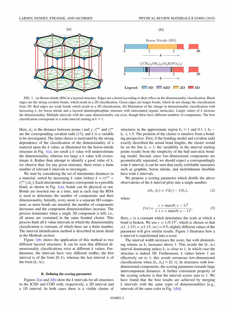
FIG. 1. (a) Boron nitride (BN) in a layered structure. Edges are colored according to their effect on the dimensionality classification. Blackedges are the strong covalent bonds, which result in a 2D classification. Green edges are longer bonds, which do not change the classificationfrom 2D. Red edges are weak bonds which result in a 3D classification. (b) Illustration of the change in dimensionality classification withincreasing k, for boron nitride and a layered aluminophosphate structure with intercalated organic molecules. Larger values of k increasethe dimensionality. Multiple intervals with the same dimensionality can exist, though these have different numbers of components. The bestclassification corresponds to a wide interval starting at k ≈ 1.

Here, di j is the distance between atoms i and j, rcovi and rcov

jare the corresponding covalent radii [13], and k is a variableto be investigated. The latter choice is motivated by the strongdependence of the classification of the dimensionality of amaterial upon the k value; as illustrated for the boron-nitridestructure in Fig. 1(a), too small a k value will underestimatethe dimensionality, whereas too large a k value will overes-timate it. Rather than attempt to identify a good value of k,we observe that, for any given structure, there exists a finitenumber of relevant k intervals to investigate.

We start by considering the set of interatomic distances ina material, sorted by increasing k value [where k = (rcov

i +rcov

j )/di j]. Each interatomic distance corresponds to a possiblebond; as shown in Fig. 1(a), bonds can be physical or not.Bonds are inserted one at a time, and at each step the RDAis used to determine the number of components and theirdimensionality. Initially, every atom is a separate 0D compo-nent; as more bonds are inserted, the number of componentsdecreases and the component dimensionalities increase. Theprocess terminates when a single 3D component is left; i.e.,all atoms are contained in the same bonded cluster. Thisprocess finds all k-value intervals in which the dimensionalityclassification is constant, of which there are a finite number.The interval identification method is described in more detailin the Methods section.

Figure 1(b) shows the application of this method to twodifferent layered structures. It can be seen that different di-mensionality classifications exist at different k values. Fur-thermore, the intervals have very different widths; the firstinterval is of the form [0, k), whereas the last interval is ofthe form [k,∞).

B. Defining the scoring parameter

Figures 2(a) and 2(b) show the k intervals for all structuresin the ICSD and COD with, respectively, a 2D interval anda 1D interval. In both cases there is a visible cluster of

structures in the approximate region k1 ≈ 1 and 0.1 � k2 −k1 � 1.5. The position of the cluster is intuitive from a bond-ing perspective. First, if the bonding model and covalent radiiexactly described the actual bond lengths, the cluster wouldlie on the line k1 = 1; the variability in the interval startingpoints results from the simplicity of the ball-and-stick bond-ing model. Second, since low-dimensional components aregeometrically separated, we should expect a correspondinglywide k interval; it can be seen that easily exfoliable structuressuch as graphite, boron nitride, and molybdenum disulfidehave wide k intervals.

We propose a scoring parameter which distills the aboveobservations of the k-interval plots into a single number:

s(k1, k2) = f (k2) − f (k1), (2)

where

f (x) = c × max(0, x − 1)2

1 + c × max(0, x − 1)2. (3)

Here, c is a constant which determines the scale at which abond is broken. We use c = 1/0.152, which is chosen so thats(1, 1.15) = s(1.15,∞) = 0.5; slightly different values of theparameter will give similar results. Figure 3 illustrates how ak interval is transformed into a score.

The interval width increases the score, but with diminish-ing returns as k1 increases above 1. This avoids the [k,∞)interval dominating unless k1 is close to 1, in which case thestructure is indeed 3D. Furthermore, k values below 1 areeffectively set to 1; this avoids erroneous low-dimensionalclassifications when [k1, k2] ≈ [0, 1]. In structures with low-dimensional components, the scoring parameter rewards largeintercomponent distances. A further convenient property ofthe scoring scheme is that the interval scores sum to 1. Wehave found that the best results are achieved by mergingk intervals with the same types of dimensionalities [e.g.,intervals of the same color in Fig. 1(b)].

034003-2

DEFINITION OF A SCORING PARAMETER TO IDENTIFY … PHYSICAL REVIEW MATERIALS 3, 034003 (2019)

(a) (b)

(c) (d)

0D 1D 2D 3D

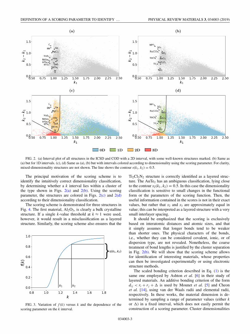
FIG. 2. (a) Interval plot of all structures in the ICSD and COD with a 2D interval, with some well-known structures marked. (b) Same as(a) but for 1D intervals. (c), (d) Same as (a), (b) but with intervals colored according to dimensionality using the scoring parameter. For clarity,mixed-dimensionality structures are not shown. The line shows the contour s(k1, k2) = 0.5.

The principal motivation of the scoring scheme is toidentify the intuitively correct dimensionality classification,by determining whether a k interval lies within a cluster ofthe type shown in Figs. 2(a) and 2(b). Using the scoringparameter, the structures are colored in Figs. 2(c) and 2(d)according to their dimensionality classification.

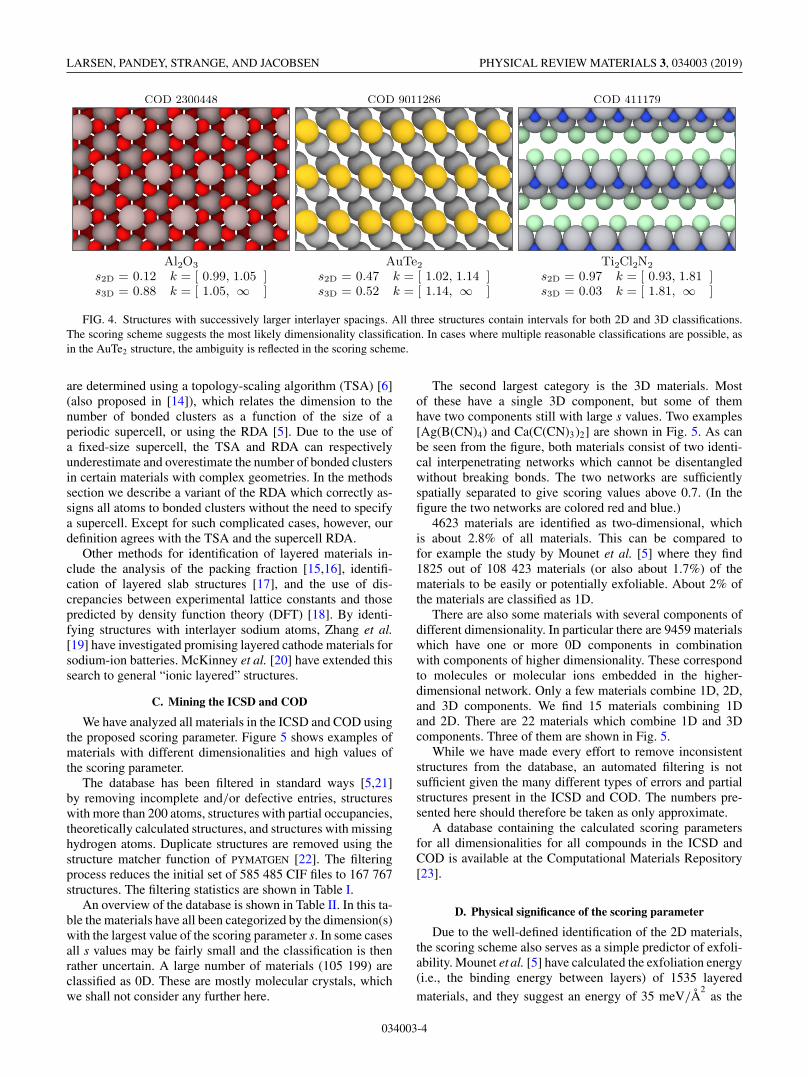
The scoring scheme is demonstrated for three structures inFig. 4. The first material, Al2O3, is clearly a bulk crystallinestructure. If a single k-value threshold at k ≈ 1 were used,however, it would result in a misclassification as a layeredstructure. Similarly, the scoring scheme also ensures that the

FIG. 3. Variation of f (k) versus k and the dependence of thescoring parameter on the k interval.

Ti2Cl2N2 structure is correctly identified as a layered struc-ture. The AuTe2 has an ambiguous classification, lying closeto the contour s2(k1, k2) = 0.5. In this case the dimensionalityclassification is sensitive to small changes in the functionalform or the parameters of the scoring function. Then, theuseful information contained in the scores is not in their exactvalues, but rather that s2 and s3 are approximately equal invalue; this can be interpreted as a layered structure with a verysmall interlayer spacing.

It should be emphasized that the scoring is exclusivelybased on interatomic distances and atomic sizes, and thatit simply assumes that longer bonds tend to be weakerthan shorter ones. The physical characters of the bonds,i.e., whether they can be considered covalent, ionic, or ofdispersion type, are not revealed. Nonetheless, the coarsetreatment of bond lengths is justified by the cluster separationin Fig. 2(b). We will show that the scoring scheme allowsfor identification of interesting materials, whose propertiescan then be investigated experimentally or using electronicstructure methods.

The scaled bonding criterion described in Eq. (1) is thesame one employed by Ashton et al. [6] in their study oflayered materials. An additive bonding criterion of the formdi j < ri + r j + � is used by Mounet et al. [5] and Cheonet al. [14], using van der Waals radii and elemental radii,respectively. In these works, the material dimension is de-termined by sampling a range of parameter values (either kor �) in a fixed interval, which does not easily permit theconstruction of a scoring parameter. Cluster dimensionalities

034003-3

LARSEN, PANDEY, STRANGE, AND JACOBSEN PHYSICAL REVIEW MATERIALS 3, 034003 (2019)

971114DOC6821109DOC8440032DOC 8440032DOC 6821109DOC 971114DOC

Al2O3 AuTe2 Ti2Cl2N2

s2D = 0.12 k = [ 0.99, 1.05 ] s2D = 0.47 k = [ 1.02, 1.14 ] s2D = 0.97 k = [ 0.93, 1.81 ]s3D = 0.88 k = [ 1.05, ∞ ] s3D = 0.52 k = [ 1.14, ∞ ] s3D = 0.03 k = [ 1.81, ∞ ]

FIG. 4. Structures with successively larger interlayer spacings. All three structures contain intervals for both 2D and 3D classifications.The scoring scheme suggests the most likely dimensionality classification. In cases where multiple reasonable classifications are possible, asin the AuTe2 structure, the ambiguity is reflected in the scoring scheme.

are determined using a topology-scaling algorithm (TSA) [6](also proposed in [14]), which relates the dimension to thenumber of bonded clusters as a function of the size of aperiodic supercell, or using the RDA [5]. Due to the use ofa fixed-size supercell, the TSA and RDA can respectivelyunderestimate and overestimate the number of bonded clustersin certain materials with complex geometries. In the methodssection we describe a variant of the RDA which correctly as-signs all atoms to bonded clusters without the need to specifya supercell. Except for such complicated cases, however, ourdefinition agrees with the TSA and the supercell RDA.

Other methods for identification of layered materials in-clude the analysis of the packing fraction [15,16], identifi-cation of layered slab structures [17], and the use of dis-crepancies between experimental lattice constants and thosepredicted by density function theory (DFT) [18]. By identi-fying structures with interlayer sodium atoms, Zhang et al.[19] have investigated promising layered cathode materials forsodium-ion batteries. McKinney et al. [20] have extended thissearch to general “ionic layered” structures.

C. Mining the ICSD and COD

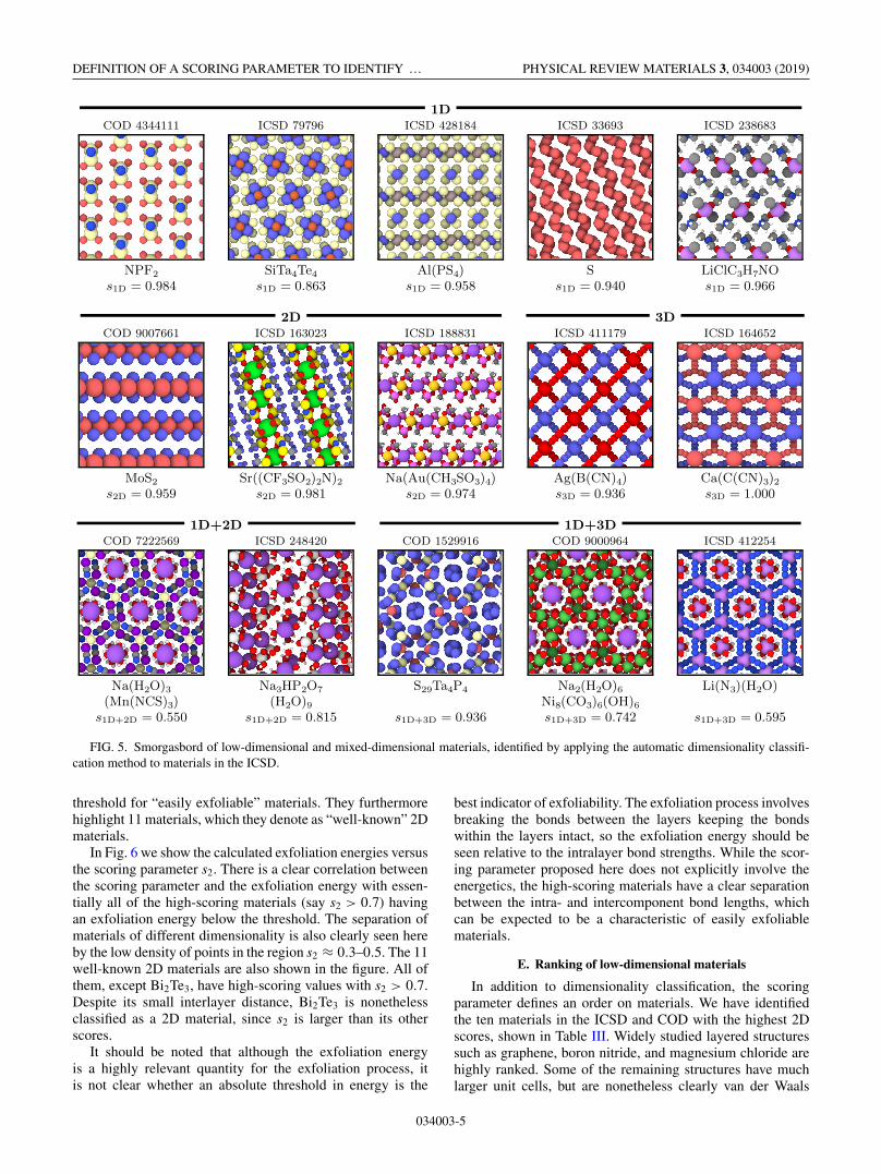
We have analyzed all materials in the ICSD and COD usingthe proposed scoring parameter. Figure 5 shows examples ofmaterials with different dimensionalities and high values ofthe scoring parameter.

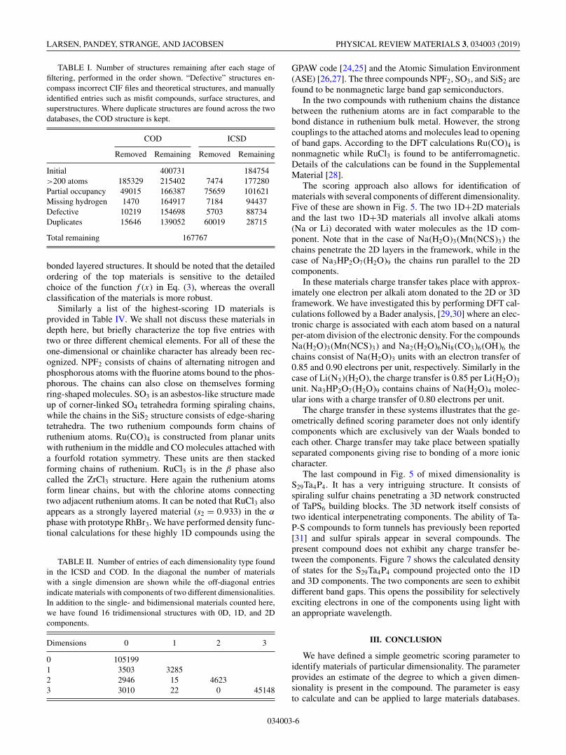
The database has been filtered in standard ways [5,21]by removing incomplete and/or defective entries, structureswith more than 200 atoms, structures with partial occupancies,theoretically calculated structures, and structures with missinghydrogen atoms. Duplicate structures are removed using thestructure matcher function of PYMATGEN [22]. The filteringprocess reduces the initial set of 585 485 CIF files to 167 767structures. The filtering statistics are shown in Table I.

An overview of the database is shown in Table II. In this ta-ble the materials have all been categorized by the dimension(s)with the largest value of the scoring parameter s. In some casesall s values may be fairly small and the classification is thenrather uncertain. A large number of materials (105 199) areclassified as 0D. These are mostly molecular crystals, whichwe shall not consider any further here.

The second largest category is the 3D materials. Mostof these have a single 3D component, but some of themhave two components still with large s values. Two examples[Ag(B(CN)4) and Ca(C(CN)3)2] are shown in Fig. 5. As canbe seen from the figure, both materials consist of two identi-cal interpenetrating networks which cannot be disentangledwithout breaking bonds. The two networks are sufficientlyspatially separated to give scoring values above 0.7. (In thefigure the two networks are colored red and blue.)

4623 materials are identified as two-dimensional, whichis about 2.8% of all materials. This can be compared tofor example the study by Mounet et al. [5] where they find1825 out of 108 423 materials (or also about 1.7%) of thematerials to be easily or potentially exfoliable. About 2% ofthe materials are classified as 1D.

There are also some materials with several components ofdifferent dimensionality. In particular there are 9459 materialswhich have one or more 0D components in combinationwith components of higher dimensionality. These correspondto molecules or molecular ions embedded in the higher-dimensional network. Only a few materials combine 1D, 2D,and 3D components. We find 15 materials combining 1Dand 2D. There are 22 materials which combine 1D and 3Dcomponents. Three of them are shown in Fig. 5.

While we have made every effort to remove inconsistentstructures from the database, an automated filtering is notsufficient given the many different types of errors and partialstructures present in the ICSD and COD. The numbers pre-sented here should therefore be taken as only approximate.

A database containing the calculated scoring parametersfor all dimensionalities for all compounds in the ICSD andCOD is available at the Computational Materials Repository[23].

D. Physical significance of the scoring parameter

Due to the well-defined identification of the 2D materials,the scoring scheme also serves as a simple predictor of exfoli-ability. Mounet et al. [5] have calculated the exfoliation energy(i.e., the binding energy between layers) of 1535 layered

materials, and they suggest an energy of 35 meV/Å2

as the

034003-4

DEFINITION OF A SCORING PARAMETER TO IDENTIFY … PHYSICAL REVIEW MATERIALS 3, 034003 (2019)

1DCOD 4344111 ICSD 79796 ICSD 428184 ICSD 33693 ICSD 238683

NPF2 SiTa4Te4 Al(PS4) S LiClC3H7NOs1D = 0.984 s1D = 0.863 s1D = 0.958 s1D = 0.940 s1D = 0.966

2D 3DCOD 9007661 ICSD 163023 ICSD 188831 ICSD 411179 ICSD 164652

MoS2 Sr((CF3SO2)2N)2 Na(Au(CH3SO3)4) Ag(B(CN)4) Ca(C(CN)3)2s2D = 0.959 s2D = 0.981 s2D = 0.974 s3D = 0.936 s3D = 1.000

1D+2D 1D+3DCOD 7222569 ICSD 248420 COD 1529916 COD 9000964 ICSD 412254

Na(H2O)3 Na3HP2O7 S29Ta4P4 Na2(H2O)6 Li(N3)(H2O)(Mn(NCS)3) (H2O)9 Ni8(CO3)6(OH)6

s1D+2D = 0.550 s1D+2D = 0.815 s1D+3D = 0.936 s1D+3D = 0.742 s1D+3D = 0.595

FIG. 5. Smorgasbord of low-dimensional and mixed-dimensional materials, identified by applying the automatic dimensionality classifi-cation method to materials in the ICSD.

threshold for “easily exfoliable” materials. They furthermorehighlight 11 materials, which they denote as “well-known” 2Dmaterials.

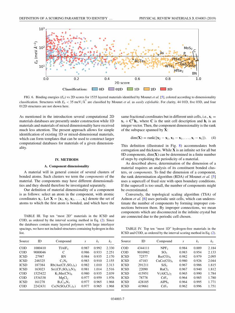
In Fig. 6 we show the calculated exfoliation energies versusthe scoring parameter s2. There is a clear correlation betweenthe scoring parameter and the exfoliation energy with essen-tially all of the high-scoring materials (say s2 > 0.7) havingan exfoliation energy below the threshold. The separation ofmaterials of different dimensionality is also clearly seen hereby the low density of points in the region s2 ≈ 0.3–0.5. The 11well-known 2D materials are also shown in the figure. All ofthem, except Bi2Te3, have high-scoring values with s2 > 0.7.Despite its small interlayer distance, Bi2Te3 is nonethelessclassified as a 2D material, since s2 is larger than its otherscores.

It should be noted that although the exfoliation energyis a highly relevant quantity for the exfoliation process, itis not clear whether an absolute threshold in energy is the

best indicator of exfoliability. The exfoliation process involvesbreaking the bonds between the layers keeping the bondswithin the layers intact, so the exfoliation energy should beseen relative to the intralayer bond strengths. While the scor-ing parameter proposed here does not explicitly involve theenergetics, the high-scoring materials have a clear separationbetween the intra- and intercomponent bond lengths, whichcan be expected to be a characteristic of easily exfoliablematerials.

E. Ranking of low-dimensional materials

In addition to dimensionality classification, the scoringparameter defines an order on materials. We have identifiedthe ten materials in the ICSD and COD with the highest 2Dscores, shown in Table III. Widely studied layered structuressuch as graphene, boron nitride, and magnesium chloride arehighly ranked. Some of the remaining structures have muchlarger unit cells, but are nonetheless clearly van der Waals

034003-5

LARSEN, PANDEY, STRANGE, AND JACOBSEN PHYSICAL REVIEW MATERIALS 3, 034003 (2019)

TABLE I. Number of structures remaining after each stage offiltering, performed in the order shown. “Defective” structures en-compass incorrect CIF files and theoretical structures, and manuallyidentified entries such as misfit compounds, surface structures, andsuperstructures. Where duplicate structures are found across the twodatabases, the COD structure is kept.

COD ICSD

Removed Remaining Removed Remaining

Initial 400731 184754>200 atoms 185329 215402 7474 177280Partial occupancy 49015 166387 75659 101621Missing hydrogen 1470 164917 7184 94437Defective 10219 154698 5703 88734Duplicates 15646 139052 60019 28715

Total remaining 167767

bonded layered structures. It should be noted that the detailedordering of the top materials is sensitive to the detailedchoice of the function f (x) in Eq. (3), whereas the overallclassification of the materials is more robust.

Similarly a list of the highest-scoring 1D materials isprovided in Table IV. We shall not discuss these materials indepth here, but briefly characterize the top five entries withtwo or three different chemical elements. For all of these theone-dimensional or chainlike character has already been rec-ognized. NPF2 consists of chains of alternating nitrogen andphosphorous atoms with the fluorine atoms bound to the phos-phorous. The chains can also close on themselves formingring-shaped molecules. SO3 is an asbestos-like structure madeup of corner-linked SO4 tetrahedra forming spiraling chains,while the chains in the SiS2 structure consists of edge-sharingtetrahedra. The two ruthenium compounds form chains ofruthenium atoms. Ru(CO)4 is constructed from planar unitswith ruthenium in the middle and CO molecules attached witha fourfold rotation symmetry. These units are then stackedforming chains of ruthenium. RuCl3 is in the β phase alsocalled the ZrCl3 structure. Here again the ruthenium atomsform linear chains, but with the chlorine atoms connectingtwo adjacent ruthenium atoms. It can be noted that RuCl3 alsoappears as a strongly layered material (s2 = 0.933) in the α

phase with prototype RhBr3. We have performed density func-tional calculations for these highly 1D compounds using the

TABLE II. Number of entries of each dimensionality type foundin the ICSD and COD. In the diagonal the number of materialswith a single dimension are shown while the off-diagonal entriesindicate materials with components of two different dimensionalities.In addition to the single- and bidimensional materials counted here,we have found 16 tridimensional structures with 0D, 1D, and 2Dcomponents.

Dimensions 0 1 2 3

0 1051991 3503 32852 2946 15 46233 3010 22 0 45148

GPAW code [24,25] and the Atomic Simulation Environment(ASE) [26,27]. The three compounds NPF2, SO3, and SiS2 arefound to be nonmagnetic large band gap semiconductors.

In the two compounds with ruthenium chains the distancebetween the ruthenium atoms are in fact comparable to thebond distance in ruthenium bulk metal. However, the strongcouplings to the attached atoms and molecules lead to openingof band gaps. According to the DFT calculations Ru(CO)4 isnonmagnetic while RuCl3 is found to be antiferromagnetic.Details of the calculations can be found in the SupplementalMaterial [28].

The scoring approach also allows for identification ofmaterials with several components of different dimensionality.Five of these are shown in Fig. 5. The two 1D+2D materialsand the last two 1D+3D materials all involve alkali atoms(Na or Li) decorated with water molecules as the 1D com-ponent. Note that in the case of Na(H2O)3(Mn(NCS)3) thechains penetrate the 2D layers in the framework, while in thecase of Na3HP2O7(H2O)9 the chains run parallel to the 2Dcomponents.

In these materials charge transfer takes place with approx-imately one electron per alkali atom donated to the 2D or 3Dframework. We have investigated this by performing DFT cal-culations followed by a Bader analysis, [29,30] where an elec-tronic charge is associated with each atom based on a naturalper-atom division of the electronic density. For the compoundsNa(H2O)3(Mn(NCS)3) and Na2(H2O)6Ni8(CO3)6(OH)6 thechains consist of Na(H2O)3 units with an electron transfer of0.85 and 0.90 electrons per unit, respectively. Similarly in thecase of Li(N3)(H2O), the charge transfer is 0.85 per Li(H2O)3

unit. Na3HP2O7(H2O)9 contains chains of Na(H2O)4 molec-ular ions with a charge transfer of 0.80 electrons per unit.

The charge transfer in these systems illustrates that the ge-ometrically defined scoring parameter does not only identifycomponents which are exclusively van der Waals bonded toeach other. Charge transfer may take place between spatiallyseparated components giving rise to bonding of a more ioniccharacter.

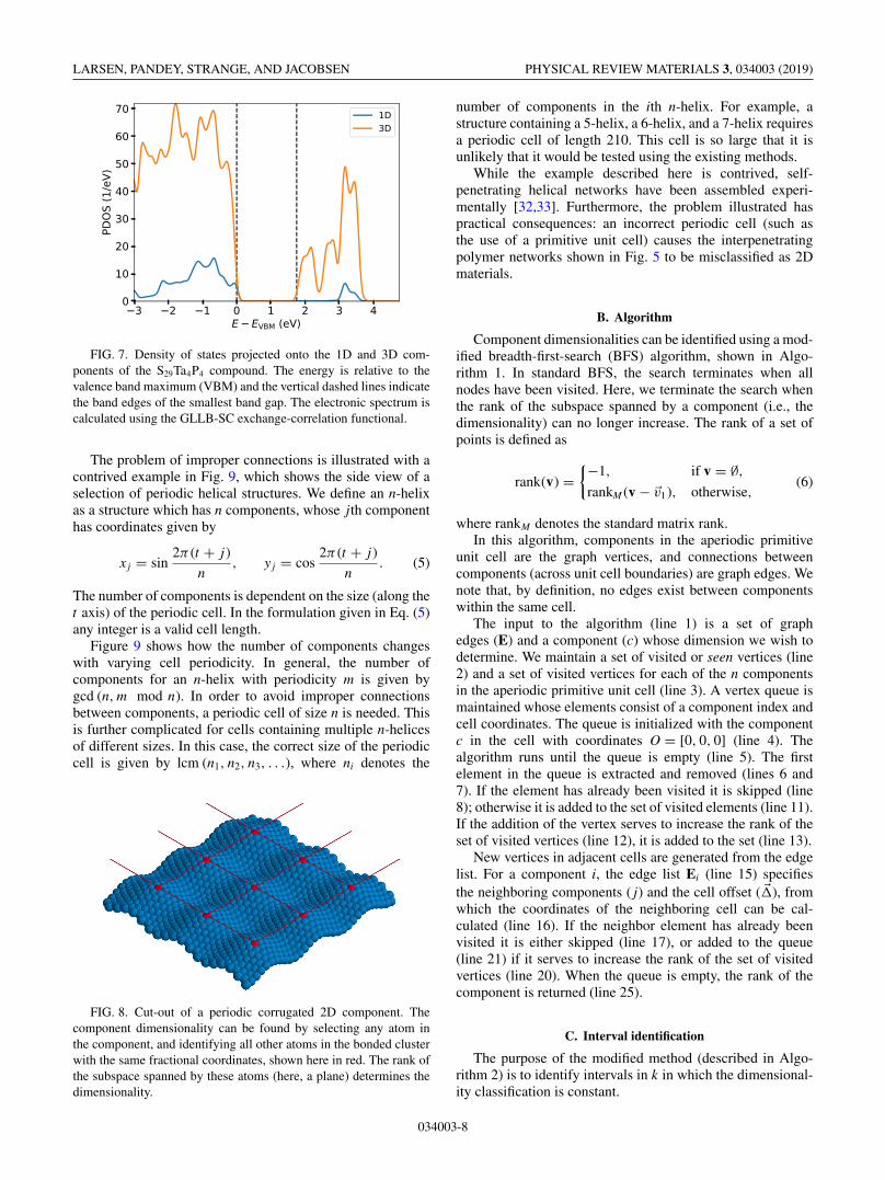
The last compound in Fig. 5 of mixed dimensionality isS29Ta4P4. It has a very intriguing structure. It consists ofspiraling sulfur chains penetrating a 3D network constructedof TaPS6 building blocks. The 3D network itself consists oftwo identical interpenetrating components. The ability of Ta-P-S compounds to form tunnels has previously been reported[31] and sulfur spirals appear in several compounds. Thepresent compound does not exhibit any charge transfer be-tween the components. Figure 7 shows the calculated densityof states for the S29Ta4P4 compound projected onto the 1Dand 3D components. The two components are seen to exhibitdifferent band gaps. This opens the possibility for selectivelyexciting electrons in one of the components using light withan appropriate wavelength.

III. CONCLUSION

We have defined a simple geometric scoring parameter toidentify materials of particular dimensionality. The parameterprovides an estimate of the degree to which a given dimen-sionality is present in the compound. The parameter is easyto calculate and can be applied to large materials databases.

034003-6

DEFINITION OF A SCORING PARAMETER TO IDENTIFY … PHYSICAL REVIEW MATERIALS 3, 034003 (2019)

Classification: 0D 02D 1D 2D 3D

FIG. 6. Binding energies (Eb) vs 2D scores for 1535 layered materials identified by Mounet et al. [5], colored according to dimensionality

classification. Structures with Eb < 35 meV/Å2

are classified by Mounet et al. as easily exfoliable. For clarity, 44 01D, five 03D, and four012D structures are not shown here.

As mentioned in the introduction several computational 2Dmaterials databases are presently under construction while 1Dmaterials and materials of mixed dimensionality have receivedmuch less attention. The present approach allows for simpleidentification of existing 1D or mixed-dimensional materials,which can form templates that can be used to construct largercomputational databases for materials of a given dimension-ality.

IV. METHODS

A. Component dimensionality

A material will in general consist of several clusters ofbonded atoms. Such clusters we term the components of thematerial. The components may have different dimensionali-ties and they should therefore be investigated separately.

Our definition of material dimensionality of a componentis as follows: select an atom in the component, with atomiccoordinates x1. Let X = {x1, x2, x3, . . . , xi} denote the set ofatoms to which the first atom is bonded, and which have the

TABLE III. Top ten “most 2D” materials in the ICSD andCOD, as ordered by the interval scoring method in Eq. (2). Sincethe databases contain many layered polymers with large interlayerspacings, we have not included structures containing hydrogen in thislist.

Source ID Compound s k1 k2

COD 1000410 TlAlF4 0.987 0.992 2.330COD 9000046 C 0.986 0.933 2.251ICSD 27987 BN 0.984 0.935 2.170ICSD 248325 C3N4 0.983 0.910 2.155ICSD 187384 Rb(Au(CF3SO3)4) 0.982 1.010 2.313ICSD 163023 Sr((CF3SO2)2N)2 0.981 1.014 2.516COD 1525422 K3Mn(CN)6 0.980 0.935 2.039COD 1534338 MgCl2 0.977 0.959 1.976ICSD 161278 B3C10N3 0.977 0.965 1.968COD 2242431 Cs(N(SO2CF3)2) 0.977 0.965 1.968

same fractional coordinates but in different unit cells, i.e., xi =x1 + CT hi, where C is the unit cell description and hi is aninteger vector. Then, the component dimensionality is the rankof the subspace spanned by X:

dim(X) = rank({x2 − x1, x3 − x1, . . . , xi − x1}). (4)

This definition (illustrated in Fig. 8) accommodates bothcorrugation and thickness. While X is an infinite set for all but0D components, dim(X) can be determined in a finite numberof steps by exploiting the periodicity of a material.

As described above, determination of the dimension of amaterial requires an analysis of its constituent bonded clus-ters, or components. To find the dimension of a component,the rank determination algorithm (RDA) of Mounet et al. [5]uses a supercell of fixed size with open boundary conditions.If the supercell is too small, the number of components mightbe overestimated.

Conversely, the topological scaling algorithm (TSA) ofAshton et al. [6] uses periodic unit cells, which can underes-timate the number of components by forming improper con-nections between them. By improper connections, we meancomponents which are disconnected in the infinite crystal butare connected due to the periodic cell chosen.

TABLE IV. Top ten “most 1D” hydrogen-free materials in theICSD and COD, as ordered by the interval scoring method in Eq. (2).

Source ID Compound s k1 k2

COD 4344111 NPF2 0.984 0.889 2.184COD 9010982 SO3 0.983 0.954 2.133ICSD 72577 Ru(CO)4 0.982 0.979 2.095ICSD 47183 CuCo(CO)4 0.980 0.926 2.044ICSD 291211 SiS2 0.967 0.986 1.815ICSD 22090 RuCl3 0.967 0.940 1.812ICSD 415951 V(AlCl4)2 0.965 0.990 1.784ICSD 78778 CrF4 0.964 0.985 1.780ICSD 428185 AlPS4 0.964 0.995 1.771ICSD 419661 CrF5 0.962 0.996 1.751

034003-7

LARSEN, PANDEY, STRANGE, AND JACOBSEN PHYSICAL REVIEW MATERIALS 3, 034003 (2019)

FIG. 7. Density of states projected onto the 1D and 3D com-ponents of the S29Ta4P4 compound. The energy is relative to thevalence band maximum (VBM) and the vertical dashed lines indicatethe band edges of the smallest band gap. The electronic spectrum iscalculated using the GLLB-SC exchange-correlation functional.

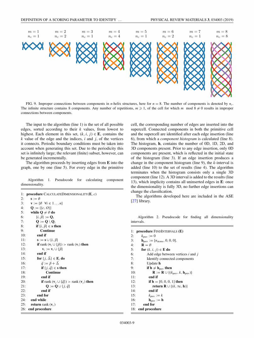
The problem of improper connections is illustrated with acontrived example in Fig. 9, which shows the side view of aselection of periodic helical structures. We define an n-helixas a structure which has n components, whose jth componenthas coordinates given by

x j = sin2π (t + j)

n, y j = cos

2π (t + j)

n. (5)

The number of components is dependent on the size (along thet axis) of the periodic cell. In the formulation given in Eq. (5)any integer is a valid cell length.

Figure 9 shows how the number of components changeswith varying cell periodicity. In general, the number ofcomponents for an n-helix with periodicity m is given bygcd (n, m mod n). In order to avoid improper connectionsbetween components, a periodic cell of size n is needed. Thisis further complicated for cells containing multiple n-helicesof different sizes. In this case, the correct size of the periodiccell is given by lcm (n1, n2, n3, . . .), where ni denotes the

FIG. 8. Cut-out of a periodic corrugated 2D component. Thecomponent dimensionality can be found by selecting any atom inthe component, and identifying all other atoms in the bonded clusterwith the same fractional coordinates, shown here in red. The rank ofthe subspace spanned by these atoms (here, a plane) determines thedimensionality.

number of components in the ith n-helix. For example, astructure containing a 5-helix, a 6-helix, and a 7-helix requiresa periodic cell of length 210. This cell is so large that it isunlikely that it would be tested using the existing methods.

While the example described here is contrived, self-penetrating helical networks have been assembled experi-mentally [32,33]. Furthermore, the problem illustrated haspractical consequences: an incorrect periodic cell (such asthe use of a primitive unit cell) causes the interpenetratingpolymer networks shown in Fig. 5 to be misclassified as 2Dmaterials.

B. Algorithm

Component dimensionalities can be identified using a mod-ified breadth-first-search (BFS) algorithm, shown in Algo-rithm 1. In standard BFS, the search terminates when allnodes have been visited. Here, we terminate the search whenthe rank of the subspace spanned by a component (i.e., thedimensionality) can no longer increase. The rank of a set ofpoints is defined as

rank(v) ={−1, if v = ∅,

rankM (v − �v1), otherwise,(6)

where rankM denotes the standard matrix rank.In this algorithm, components in the aperiodic primitive

unit cell are the graph vertices, and connections betweencomponents (across unit cell boundaries) are graph edges. Wenote that, by definition, no edges exist between componentswithin the same cell.

The input to the algorithm (line 1) is a set of graphedges (E) and a component (c) whose dimension we wish todetermine. We maintain a set of visited or seen vertices (line2) and a set of visited vertices for each of the n componentsin the aperiodic primitive unit cell (line 3). A vertex queue ismaintained whose elements consist of a component index andcell coordinates. The queue is initialized with the componentc in the cell with coordinates O = [0, 0, 0] (line 4). Thealgorithm runs until the queue is empty (line 5). The firstelement in the queue is extracted and removed (lines 6 and7). If the element has already been visited it is skipped (line8); otherwise it is added to the set of visited elements (line 11).If the addition of the vertex serves to increase the rank of theset of visited vertices (line 12), it is added to the set (line 13).

New vertices in adjacent cells are generated from the edgelist. For a component i, the edge list Ei (line 15) specifiesthe neighboring components ( j) and the cell offset (��), fromwhich the coordinates of the neighboring cell can be cal-culated (line 16). If the neighbor element has already beenvisited it is either skipped (line 17), or added to the queue(line 21) if it serves to increase the rank of the set of visitedvertices (line 20). When the queue is empty, the rank of thecomponent is returned (line 25).

C. Interval identification

The purpose of the modified method (described in Algo-rithm 2) is to identify intervals in k in which the dimensional-ity classification is constant.

034003-8

DEFINITION OF A SCORING PARAMETER TO IDENTIFY … PHYSICAL REVIEW MATERIALS 3, 034003 (2019)

m = 1 m = 2 m = 3 m = 4 m = 5 m = 6 m = 7 m = 8nc = 1 nc = 2 nc = 1 nc = 4 nc = 1 nc = 2 nc = 1 nc = 8

FIG. 9. Improper connections between components in n-helix structures, here for n = 8. The number of components is denoted by nc.The infinite structure contains 8 components. Any number of repetitions, m � 1, of the cell for which m mod 8 �= 0 results in improperconnections between components.

The input to the algorithm (line 1) is the set of all possibleedges, sorted according to their k values, from lowest tohighest. Each element in this set, (k, i, j) ∈ E, contains thek value of the edge and the indices, i and j, of the verticesit connects. Periodic boundary conditions must be taken intoaccount when generating this set. Due to the periodicity thisset is infinitely large; the relevant (finite) subset, however, canbe generated incrementally.

The algorithm proceeds by inserting edges from E into thegraph, one by one (line 5). For every edge in the primitive

Algorithm 1. Pseudocode for calculating componentdimensionality.

1: procedure CALCULATEDIMENSIONALITY(E, c)2: s := ∅3: v := {∅ ∀i ∈ 1 . . . n}4: Q := {{c, O}}5: while Q �= ∅ do6: {i,�p} := Q1

7: Q := Q \ Q1

8: if {i,�p} ∈ s then9: Continue10: end if11: s := s ∪ {i,�p}12: if rank (vi ∪ {�p}) > rank (vi ) then13: vi := vi ∪ {�p}14: end if15: for { j, ��} ∈ Ei do16: �q := �p + ��17: if { j,�q} ∈ s then18: Continue19: end if20: if rank (v j ∪ {�q}) > rank (v j ) then21: Q := Q ∪ { j,�q}22: end if23: end for24: end while25: return rank (vc )26: end procedure

cell, the corresponding number of edges are inserted into thesupercell. Connected components in both the primitive celland the supercell are identified after each edge insertion (line6), from which a component histogram is calculated (line 8).The histogram, h, contains the number of 0D, 1D, 2D, and3D components present. Prior to any edge insertion, only 0Dcomponents are present, which is reflected in the initial stateof the histogram (line 3). If an edge insertion produces achange in the component histogram (line 9), the k-interval isadded (line 10) to the set of results (line 4). The algorithmterminates when the histogram consists only a single 3Dcomponent (line 12). A 3D interval is added to the results (line13), which implicity contains all uninserted edges in E: oncethe dimensionality is fully 3D, no further edge insertions canchange the classification.

The algorithms developed here are included in the ASE[27] library.

Algorithm 2. Pseudocode for finding all dimensionalityintervals.

1: procedure FINDINTERVALS (E)2: kprev := 03: hprev := [natoms, 0, 0, 0].4: R = ∅5: for (k, i, j) ∈ E do6: Add edge between vertices i and j7: Identify connected components8: Update h9: if h �= hprev then10: R := R ∪ {(kprev, k, hprev)}11: end if12: if h = [0, 0, 0, 1] then13: return R ∪ {(k,∞, h)}14: end if15: kprev := k16: hprev := h17: end for18: end procedure

034003-9

LARSEN, PANDEY, STRANGE, AND JACOBSEN PHYSICAL REVIEW MATERIALS 3, 034003 (2019)

ACKNOWLEDGMENTS

The authors thank Nicolas Mounet and Nicola Marzari forkindly providing data for the layered compounds identifiedby Mounet et al. [5], FIZ Karlsruhe–Leibniz Institute forInformation Infrastructure for providing CIF files of all entries

in the ICSD, and anonymous referees for comments whichimproved the manuscript. This work was supported by GrantNo. 7026-00126B from the Danish Council for IndependentResearch and by the VILLUM Center for Science of Sustain-able Fuels and Chemicals which is funded by the VILLUMFonden research grant (9455).

[1] K. S. Novoselov, A. K. Geim, S. V. Morozov, D. Jiang, Y.Zhang, S. V. Dubonos, I. V. Grigorieva, and A. A. Firsov,Science 306, 666 (2004).

[2] G. R. Bhimanapati, Z. Lin, V. Meunier, Y. Jung, J. Cha, S. Das,D. Xiao, Y. Son, M. S. Strano, V. R. Cooper, L. Liang, S. G.Louie, E. Ringe, W. Zhou, S. S. Kim, R. R. Naik, B. G. Sumpter,H. Terrones, F. Xia, Y. Wang, J. Zhu, D. Akinwande, N. Alem,J. A. Schuller, R. E. Schaak, M. Terrones, and J. A. Robinson,ACS Nano 9, 11509 (2015).

[3] A. C. Ferrari, F. Bonaccorso, V. Fal’ko, K. S. Novoselov, S.Roche, P. Bøggild, S. Borini, F. H. L. Koppens, V. Palermo,N. Pugno, J. A. Garrido, R. Sordan, A. Bianco, L. Ballerini,M. Prato, E. Lidorikis, J. Kivioja, C. Marinelli, T. Ryhänen, A.Morpurgo, J. N. Coleman, V. Nicolosi, L. Colombo, A. Fert,M. Garcia-Hernandez, A. Bachtold, G. F. Schneider, F. Guinea,C. Dekker, M. Barbone, Z. Sun, C. Galiotis, A. N. Grigorenko,G. Konstantatos, A. Kis, M. Katsnelson, L. Vandersypen, A.Loiseau, V. Morandi, D. Neumaier, E. Treossi, V. Pellegrini,M. Polini, A. Tredicucci, G. M. Williams, B. Hee Hong, J.-H.Ahn, J. Min Kim, H. Zirath, B. J. van Wees, H. van der Zant, L.Occhipinti, A. Di Matteo, I. A. Kinloch, T. Seyller, E. Quesnel,X. Feng, K. Teo, N. Rupesinghe, P. Hakonen, S. R. T. Neil,Q. Tannock, T. Löfwander, and J. Kinaret, Nanoscale 7, 4598(2015).

[4] M. Zeng, Y. Xiao, J. Liu, K. Yang, and L. Fu, Chem. Rev. 118,6236 (2018).

[5] N. Mounet, M. Gibertini, P. Schwaller, D. Campi, A.Merkys, A. Marrazzo, T. Sohier, I. E. Castelli, A. Cepellotti,G. Pizzi, and N. Marzari, Nat. Nanotechnol. 13, 246(2018).

[6] M. Ashton, J. Paul, S. B. Sinnott, and R. G. Hennig, Phys. Rev.Lett. 118, 106101 (2017).

[7] S. Haastrup, M. Strange, M. Pandey, T. Deilmann, P. S.Schmidt, N. F. Hinsche, M. N. Gjerding, D. Torelli, P. M.Larsen, A. C. Riis-Jensen, J. Gath, K. W. Jacobsen, J. J.Mortensen, T. Olsen, and K. S. Thygesen, 2D Mater. 5, 042002(2018).

[8] M. A. Stolyarov, G. Liu, M. A. Bloodgood, E. Aytan, C. Jiang,R. Samnakay, T. T. Salguero, D. L. Nika, S. L. Rumyantsev,M. S. Shur, K. N. Bozhilov, and A. A. Balandin, Nanoscale 8,15774 (2016).

[9] A. Geremew, M. A. Bloodgood, E. Aytan, B. W. K. Woo, S. R.Corber, G. Liu, K. Bozhilov, T. T. Salguero, S. Rumyantsev,M. P. Rao, and A. A. Balandin, IEEE Electron Devices Lett. 39,735 (2018).

[10] D. Jariwala, T. J. Marks, and M. C. Hersam, Nat. Mater. 16, 170(2017).

[11] G. Bergerhoff, R. Hundt, R. Sievers, and I. Brown, J. Chem. Inf.Comput. Sci. 23, 66 (1983).

[12] S. Gražulis, A. Daškevic, A. Merkys, D. Chateigner, L.Lutterotti, M. Quirós, N. R. Serebryanaya, P. Moeck, R. T.Downs, and A. Le Bail, Nucleic Acids Res. 40, D420 (2012).

[13] B. Cordero, V. Gómez, A. E. Platero-Prats, M. Revés, J.Echeverría, E. Cremades, F. Barragán, and S. Alvarez, DaltonTrans. 2008, 2832.

[14] G. Cheon, K.-A. N. Duerloo, A. D. Sendek, C. Porter, Y. Chen,and E. J. Reed, Nano Lett. 17, 1915 (2017).

[15] T. Björkman, A. Gulans, A. V. Krasheninnikov, and R. M.Nieminen, Phys. Rev. Lett. 108, 235502 (2012).

[16] S. Lebègue, T. Björkman, M. Klintenberg, R. M. Nieminen, andO. Eriksson, Phys. Rev. X 3, 031002 (2013).

[17] P. Gorai, E. S. Toberer, and V. Stevanovic, J. Mater. Chem. A 4,11110 (2016).

[18] K. Choudhary, I. Kalish, R. Beams, and F. Tavazza, Sci. Rep. 7,5179 (2017).

[19] X. Zhang, Z. Zhang, S. Yao, A. Chen, X. Zhao, and Z. Zhou,npj Comput. Mater. 4, 13 (2018).

[20] R. McKinney, P. Gorai, S. Manna, E. Toberer, and V.Stevanovic, J. Mater. Chem. A 6, 15828 (2018).

[21] S. Kirklin, J. E. Saal, B. Meredig, A. Thompson, J. W. Doak, M.Aykol, S. Rühl, and C. Wolverton, npj Comput. Mater. 1, 15010(2015).

[22] S. P. Ong, W. D. Richards, A. Jain, G. Hautier, M. Kocher, S.Cholia, D. Gunter, V. L. Chevrier, K. A. Persson, and G. Ceder,Comput. Mater. Sci. 68, 314 (2013).

[23] Computational Materials Repository, https://cmr.fysik.dtu.dk/lowdim/lowdim.html.

[24] J. J. Mortensen, L. B. Hansen, and K. W. Jacobsen, Phys. Rev.B 71, 035109 (2005).

[25] J. Enkovaara, C. Rostgaard, J. J. Mortensen, J. Chen, M. Dułak,L. Ferrighi, J. Gavnholt, C. Glinsvad, V. Haikola, H. A. Hansen,H. H. Kristoffersen, M. Kuisma, A. H. Larsen, L. Lehtovaara,M. Ljungberg, O. Lopez-Acevedo, P. G. Moses, J. Ojanen,T. Olsen, V. Petzold, N. A. Romero, J. Stausholm-Møller, M.Strange, G. A. Tritsaris, M. Vanin, M. Walter, B. Hammer, H.Hakkinen, G. K. H. Madsen, R. M. Nieminen, J. K. Nørskov,M. Puska, T. T. Rantala, J. Schiøtz, K. S. Thygesen, and K. W.Jacobsen, J. Phys.: Condens. Matter 22, 3202 (2010).

[26] S. R. Bahn and K. W. Jacobsen, Comput. Sci. Eng. 4, 56(2002).

[27] A. Larsen, J. Mortensen, J. Blomqvist, I. E. Castelli, R.Christensen, M. Dulak, J. Friis, M. Groves, B. Hammer, C.Hargus, E. Hermes, P. Jennings, P. Jensen, J. Kermode, J.Kitchin, E. Kolsbjerg, J. Kubal, K. Kaasbjerg, S. Lysgaard, J.Maronsson, T. Maxson, T. Olsen, L. Pastewka, A. Peterson, C.Rostgaard, J. Schiøtz, O. Schütt, M. Strange, K. S. Thygesen, T.Vegge, L. Vilhelmsen, M. Walter, Z. Zeng, and K. W. Jacobsen,J. Phys.: Condens. Matter 29, 273002 (2017).

034003-10

DEFINITION OF A SCORING PARAMETER TO IDENTIFY … PHYSICAL REVIEW MATERIALS 3, 034003 (2019)

[28] See Supplemental Material at http://link.aps.org/supplemental/10.1103/PhysRevMaterials.3.034003 for DFT-calculated elec-tronic spectra.

[29] R. F. W. Bader and R. F. Bader, Atoms in Molecules: A Quan-tum Theory, International Series of Monographs on Chemistry(Clarendon Press, Oxford, 1990).

[30] W. Tang, E. Sanville, and G. Henkelman, J. Phys.: Condens.Matter 21, 084204 (2009).

[31] M. Evain, S. Lee, M. Queignec, and R. Brec, J. Solid StateChem. 71, 139 (1987).

[32] D.-R. Xiao, Y.-G. Li, E.-B. Wang, L.-L. Fan, H.-Y.An, Z.-M. Su, and L. Xu, Inorg. Chem. 46, 4158(2007).

[33] G.-P. Yang, L. Hou, X.-J. Luan, B. Wu, and Y.-Y. Wang, Chem.Soc. Rev. 41, 6992 (2012).

034003-11