1

Decentralized Rigidity Maintenance Control withRange Measurements for Multi-Robot Systems

Daniel Zelazo, Antonio Franchi, Heinrich H. Bulthoff, and Paolo Robuffo Giordano

Abstract—This work proposes a fully decentralized strategyfor maintaining the formation rigidity of a multi-robot systemusing only range measurements, while still allowing the graphtopology to change freely over time. In this direction, a firstcontribution of this work is an extension of rigidity theory toweighted frameworks and the rigidity eigenvalue, which whenpositive ensures the infinitesimal rigidity of the framework. Wethen propose a distributed algorithm for estimating a commonrelative position reference frame amongst a team of robots withonly range measurements in addition to one agent endowed withthe capability of measuring the bearing to two other agents. Thisfirst estimation step is embedded into a subsequent distributedalgorithm for estimating the rigidity eigenvalue associated withthe weighted framework. The estimate of the rigidity eigenvalue isfinally used to generate a local control action for each agent thatboth maintains the rigidity property and enforces additional con-straints such as collision avoidance and sensing/communicationrange limits and occlusions. As an additional feature of ourapproach, the communication and sensing links among therobots are also left free to change over time while preservingrigidity of the whole framework. The proposed scheme is thenexperimentally validated with a robotic testbed consisting of 6quadrotor UAVs operating in a cluttered environment.

Index Terms—graph rigidity, decentralized control, multi-robot, distributed algorithms, distributed estimation.

I. INTRODUCTION

The coordinated and decentralized control of multi-robotsystems is an enabling technology for a variety of applications.Multi-robot systems benefit from an increased robustnessagainst system failures due to their ability to adapt to dy-namic and uncertain environments. There are also numerouseconomic benefits by considering the price of small and cost-effective autonomous systems as opposed to their more expen-sive monolithic counterparts. Currently, there is a great interestin implementing these systems from deep space interferometrymissions and distributed sensing and data collection, to civiliansearch and rescue operations, among others (Akyildiz et al.,2002; Anderson et al., 2008a; Bristow et al., 2000; Lindseyet al., 2011; Mesbahi and Egerstedt, 2010; Michael et al.,2009; Murray, 2006).

D. Zelazo is with the Faculty of Aerospace Engineering, Technion - IsraelInstitute of Technology, Haifa 32000, Israel dzelazo@technion.ac.il

A Franchi is with the Centre National de la Recherche Scien-tifique (CNRS), Laboratoire d’Analyse et d’Architecture des Systemes(LAAS), 7 Avenue du Colonel Roche, 31077 Toulouse CEDEX 4, France.antonio.franchi@laas.fr

H. H. Bulthoff is with the Max Planck Institute for Biological Cybernetics,Spemannstraße 38, 72076 Tubingen, Germany hhb@tuebingen.mpg.de.H. H. Bulthoff is additionally with the Department of Brain and CognitiveEngineering, Korea University, Seoul, 136-713 Korea.

P. Robuffo Giordano is with the CNRS at Irisa and Inria RennesBretagne Atlantique, Campus de Beaulieu, 35042 Rennes Cedex, Franceprg@irisa.fr.

The challenges associated with the design and implemen-tation of multi-agent systems range from hardware and soft-ware considerations to the development of a solid theoreticalfoundation for their operation. In particular, the sensing andcommunication capabilities of each agent will dictate thedistributed protocols used to achieve team objectives. Forexample, if each agent in a multi-robot system is equippedwith a GPS-like sensor, then tasks such as formation keepingor localization can be trivially accomplished by communica-tion between robots of their state information in a commonworld-frame. However, in applications operating in harsherenvironments, i.e., indoors, underwater, or in deep-space, GPSis not a viable sensing option (Scaramuzza et al., 2014).Indeed, in these situations, agents must rely on sensing withoutknowledge of a common inertial reference frame (Franchiet al., 2012a). In these scenarios, relative sensing can provideaccurate measurements of, for example, range or bearing, butwithout any common reference frame.

A further challenge related to the sensing capabilities ofmulti-robot systems is the availability of these measurements.Sensing constraints such as line-of-sight requirements, range,and power limitations introduce an important system-levelrequirement, and also lead to an inherently time-varyingdescription of the sensing network. Successful decentralizedcoordination protocols, therefore, must also be able to managethese constraints.

These issues lead to important architectural requirements forthe sensing and communication topology in order to achievethe desired higher level tasks (i.e., formation keeping or local-ization). The connectivity of the sensing and communicationtopology is one such property that has received considerableattention in the multi-robot communities (Robuffo Giordanoet al., 2011, 2013; Ji and Egerstedt, 2007). However, con-nectivity alone is not sufficient to perform certain tasks whenonly relative sensing is used. For these systems, the conceptof rigidity provides the correct framework for defining anappropriate sensing and communication topology architecture.Rigidity is a combinatorial theory for characterizing the “stiff-ness” or “flexibility” of structures formed by rigid bodiesconnected by flexible linkages or hinges.

The study of rigidity has a rich history with contributionsfrom mathematics and engineering disciplines (Connelly andWhiteley, 2009; Jacobs, 1997; Krick et al., 2009; Laman,1970; Shames et al., 2009; Tay and Whiteley, 1985; Erenet al., 2004). Recently, rigidity theory has taken an outstandingrole in the motion control of mobile robots. The rigidityframework allows for applications, such as formation control,to employ control algorithms relying on only relative distancemeasurements, as opposed to relative position measurements

arX

iv:1

309.

0535

v3 [

cs.S

Y]

4 S

ep 2

014

2

from a global or relative internal frame (Anderson et al.,2008a,b; Baillieul and McCoy, 2007; Krick et al., 2009; Olfati-Saber and Murray, 2002; Smith et al., 2007). For example, in(Krick et al., 2009) it was shown that formation stabilizationusing only distance measurements can be achieved only ifrigidity of the formation is maintained. Moreover, rigidityrepresents also a necessary condition for estimating relativepositions using only relative distance measurements (Aspneset al., 2006; Calafiore et al., 2010a).

In a broader context, rigidity turns out to be an importantarchitectural property of many multi-agent systems when acommon inertial reference frame is unavailable. Applicationsthat rely on sensor fusion for localization, exploration, map-ping and cooperative tracking of a target, all can benefitfrom notions in rigidity theory (Shames et al., 2009; Aspneset al., 2006; Calafiore et al., 2010b; Williams et al., 2014; Wuet al., 2010). The concept of rigidity, therefore, provides thetheoretical foundation for approaching decentralized solutionsto the aforementioned problems using distance measurementsensors, and thus establishing an appropriate framework forrelating system level architectural requirements to the sensingand communication capabilities of the system.

A. Main Contributions

In general, rigidity as a property of a given formation(i.e., of the robot spatial arrangement) has been studied fromeither a purely combinatorial perspective (Laman, 1970), or byproviding an algebraic characterization via the state-dependentrigidity matrix (Tay and Whiteley, 1985). In our previous work(Zelazo et al., 2012), we introduced a related matrix termedthe symmetric rigidity matrix. A main result of (Zelazo et al.,2012) was to provide a necessary and sufficient conditions forrigidity in the plane in terms of the positivity of a particulareigenvalue of the symmetric rigidity matrix; this eigenvaluewe term the rigidity eigenvalue. This result is in the samespirit as the celebrated Fiedler eigenvalue1 and its relation tothe connectivity of a graph (Godsil and Royle, 2001). A firstcontribution of this work is the extension of the results onthe rigidity eigenvalue provided in (Zelazo et al., 2012) to3-dimensional frameworks, as well as the introduction of theconcept of weighted rigidity and the corresponding weightedrigidity matrix. This notion allows for the concept of rigidityto include state-dependent weight functions on the edges ofthe graph, weights which can then be exploited to take intoaccount inter-agent sensing and communication constraintsand/or requirements.

A gradient-based rigidity maintenance action aimed at‘maximizing’ the rigidity eigenvalue was also proposed in (Ze-lazo et al., 2012). However, while this gradient control law wasdecentralized in structure, there was still a dependence on theavailability of several global quantities, namely, of the robotrelative positions in some common reference frame, of thevalue of the rigidity eigenvalue, and of the rigidity eigenvectorassociated with the rigidity eigenvalue. A main contribution ofthis work is then the development of the machinery needed todistributedly estimate all these global quantities by resorting

1The second smallest eigenvalue of the graph Laplacian matrix.

to only relative distance measurements among neighbors, soas to ultimately allow for a fully distributed and range-basedimplementation of the rigidity maintenance controller. To thisend, we first show that if the formation is infinitesimally rigid,it is possible to distributedly estimate the relative positions ofneighboring robots in a common reference frame from onlyrange-based measurements. Our approach relies explicitly onthe form of the symmetric rigidity matrix developed here,in contrast to other approaches focusing on distributed im-plementations of centralized estimation schemes, such as aGauss-Newton approach used in Calafiore et al. (2010b).Thisfirst step is then instrumental for the subsequent developmentof the distributed estimation of the rigidity eigenvalue andeigenvector needed by the rigidity gradient controller. Thisis obtained by exploiting an appropriate modification of thepower iteration method for eigenvalue estimation followingfrom the works (Robuffo Giordano et al., 2011; Yang et al.,2010) for the distributed estimation of the connectivity eigen-value of the graph Laplacian and now applied to rigidity.Finally, we show how to exploit the weights on the graph edgesto embed constraints and requirements such as inter-robotand obstacle avoidance, limited communication and sensingranges, and line-of-sight occlusions, into a unified gradient-based rigidity maintenance control law.

Our approach, therefore, can be considered as a contributionto the general problem of distributed strategies for maintainingcertain architectural features of a multi-robot system (i.e. con-nectivity or rigidity) with minimal sensing requirements (onlyrelative distance measurements). Additionally, we also providea thorough experimental validation of the entire framework byemploying a group of 6 quadrotor UAVs as robotic platformsto demonstrate the feasibility of our approach in real-worldconditions.

The organization of this paper is as follows. Section I-Bprovides a brief overview of some notation and fundamentaltheoretical properties of graphs. In Section II, the theoryof rigidity is introduced, and our extension of the rigidityeigenvalue to 3-dimensional weighted frameworks is given.We then proceed to present a general strategy for a distributedrigidity maintenance controller in Section III. This sectionwill provide details on certain operational constraints of themulti-robot team and how these constraints can be embeddedin the control law. This section also highlights the needto develop distributed algorithms for estimating a commonreference frame for the team, outlined in Section IV, andestimation of the rigidity eigenvalue and eigenvector, detailedin Section V. The results of the previous sections are thensummarized in Section VI where the full distributed rigiditymaintenance controller is given. The applicability of theseresults are then experimentally demonstrated on a robotictestbed consisting of 6 quadrotor UAVs operating in a obstaclepopulated environment. Details of the experimental setup andresults are given in Section VII. Finally, some concludingremarks are offered in Section VIII.

B. Preliminaries and NotationsThe notation employed is standard. Matrices are denoted

by capital letters (e.g., A), and vectors by lower case letters

3

(e.g., x). The ij-th entry of a matrix A is denoted [A]ij . Therank of a matrix A is denoted rk[A]. Diagonal matrices willbe written as D = diag{d1, . . . , dn}; this notation will alsobe employed for block-diagonal matrices. A matrix and/or avector that consists of all zero entries will be denoted by 0;whereas, ‘0’ will simply denote the scalar zero. Similarly, thevector 1n denotes the n× 1 vector of all ones. The n × nidentity matrix is denoted as In. The set of real numbers willbe denoted as R, and ‖ · ‖ denotes the standard Euclidean2-norm for vectors. The Kronecker product of two matrices Aand B is written as A⊗B (Horn and Johnson, 1991).

Graphs and the matrices associated with them will be widelyused in this work; see, e.g., (Godsil and Royle, 2001). Anundirected (simple) weighted graph G is specified by a vertexset V , an edge set E whose elements characterize the incidencerelation between distinct pairs of V , and diagonal |E| × |E|weight-matrix W , with [W ]kk ≥ 0 the weight on edge ek ∈ E .In this work we consider only finite graphs and denote thecardinality of the node and edge sets as |V| = n and |E| = m.Two vertices i and j are called adjacent (or neighbors) when{i, j} ∈ E .The neighborhood of the vertex i is the set Ni ={j ∈ V | {i, j} ∈ E}. An orientation of an undirected graph Gis the assignment of directions to its edges, i.e., an edge ek isan ordered pair (i, j) such that i and j are, respectively, theinitial and the terminal nodes of ek.

The incidence matrix E(G) ∈ Rn×m is a {0,±1}-matrixwith rows and columns indexed by the vertices and edgesof G such that [E(G)]ik has the value ‘+1’ if node i is theinitial node of edge ek, ‘−1’ if it is the terminal node, and‘0’ otherwise. The degree of vertex i, di, is the cardinality ofthe set of vertices adjacent to it. The degree matrix, ∆(G),and the adjacency matrix, A(G), are defined in the usualway (Godsil and Royle, 2001). The (graph) Laplacian ofG, L(G) = E(G)E(G)T = ∆(G) − A(G), is a positive-semidefinite matrix. One of the most important results fromalgebraic graph theory in the context of collective motioncontrol states that a graph is connected if and only if thesecond smallest eigenvalue of the Laplacian is positive (Godsiland Royle, 2001).

Table I provides a summary of the notations used throughoutthe document.

II. RIGIDITY AND THE RIGIDITY EIGENVALUE

In this section we review the fundamental concepts of graphrigidity (Graver et al., 1993; Jackson, 2007). A contributionof this work is an extension of our previous results onthe concepts of the symmetric rigidity matrix and rigidityeigenvalue for 3-dimensional ambient spaces (Zelazo et al.,2012), and the notion of weighted frameworks.

A. Graph Rigidity and the Rigidity Matrix

We consider graph rigidity from what is known as a d-dimensional bar-and-joint framework. A framework is the pair(G, p), where G = (V, E) is a graph, and p : V → Rdmaps each vertex to a point in Rd. In this work we considerframeworks in a three-dimensional ambient space, i.e., d = 3.Therefore, for node u ∈ V , p(u) =

[pxu pyu pzu

]Tis

the position vector in R3 for the mapped node. We refer tothe matrix p(V) =

[p(v1) · · · p(vn)

]T ∈ Rn×3 as theposition matrix. We now provide some basic definitions.

Definition II.1. Frameworks (G, p0) and (G, p1) are equiva-lent if ‖p0(u)− p0(v)‖ = ‖p1(u)− p1(v)‖ for all {u, v} ∈ E ,and are congruent if ‖p0(u)− p0(v)‖ = ‖p1(u)− p1(v)‖ forall {u, v} ∈ V .

Definition II.2. A framework (G, p0) is globally rigid if everyframework which is equivalent to (G, p0) is congruent to(G, p0).

Definition II.3. A framework (G, p0) is rigid if there exists anε > 0 such that every framework (G, p1) which is equivalentto (G, p0) and satisfies ‖p0(v)− p1(v)‖ < ε for all v ∈ V , iscongruent to (G, p0).

Definition II.4. A minimally rigid graph is a rigid graph suchthat the removal of any edge results in a non-rigid graph.

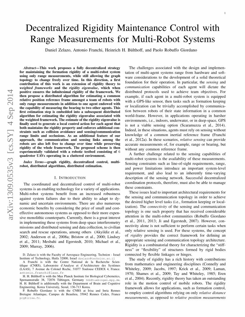
Figure 1 shows three frameworks illustrating the abovedefinitions. The frameworks in Figure 1(a) are both minimallyrigid and are equivalent to each other, but are not congruent,and therefore not globally rigid. By adding an additional edge,as in Figure 1(b) (the edge {v4, v5}), the framework becomesglobally rigid. The key feature of global rigidity, therefore, isthat the distances between all node pairs are maintained fordifferent framework realizations, and not just those defined bythe edge set.

By parameterizing the position map by a positive scalarrepresenting time, we can also consider trajectories of a frame-work. That is, the position map now becomes p : V×R→ R3

and is assumed to be continuously differentiable with respectto time. We then explicitly write (G, p, t) so as to representa time-varying framework. In this direction, we can define a

TABLE INOTATIONS

G = (V, E) a graph defined by its vertex and edge setsNi(t) time-varying neighborhood of node vi ∈ Vp(i) position vector in R3 of the mapped node vi ∈ V;psi s ∈ {x, y, z} coordinate of position vector for node ip(V) stacked position matrix of all nodes (Rn×3)ξ(i) velocity vector in R3 of the node vi ∈ V

(G, p,W) a weighted frameworkR(p,W) rigidity matrix of a weighted frameworkR symmetric rigidity matrix of a weighted framework

λ7, v7 (v) rigidity eigenvalue and eigenvector`ij distance between nodes vi, vj ∈ V , i.e., ‖p(vi)− p(vj)‖λi7 agent i’s estimate of the rigidity eigenvaluevsi s-coordinate of the agent i estimation

of the rigidity eigenvectorpi,c agent i estimate of relative position vector pi − pcp stacked vector of the relative

position vector estimate pi − pc, i = 1 . . . n

avg(x) the average of a vector x ∈ Rn, avg(x) = 1n

∑ni=1 xi

vxi agent i estimate of avg(vx)v2xi agent i estimate of avg(vx ◦ vx)zxyi agent i estimate of avg(py,c ◦ vx − px,c ◦ vy)zxzi agent i estimate of avg(pz,c ◦ vx − px,c ◦ vz)zyzi agent i estimate of avg(py,c ◦ vz − pz,c ◦ vy)

4

v4

v1v2

v5

v3

v3

v1 v2

v4

v1v2

v5

v3

v3

v1 v2

(a) Two equivalent minimally rigid frameworks in R3. The framework on theright side is obtained by the reflection of the position of v5 with respect tothe plane characterized by the positions of v1, v2, and v3 (as illustrated ingrey).

v4

v1v2

v5

v3

v3

v1 v2

(b) An infinitesimally and globallyrigid framework in R3.

v1v2

v3{v1, v2} {v2, v3}

{v1, v3}

(c) A non-infinitesimally rigid frame-work (note that vertexes v1 and v3 areconnected).

Fig. 1. Examples of rigid and infinitesimally rigid frameworks in R3. Noticethat in Figs. (a) and (b) the 3D points associated to each vertex do not lie onthe same plane, while in Fig. (c) the 3D points are aligned.

set of trajectories that are edge-length preserving, in the sensethat for each time t ≥ t0, the framework (G, p, t) is equivalentto the framework (G, p, t0). More formally, an edge-lengthpreserving framework must satisfy the constraint

‖p(v, t)− p(u, t)‖ = ‖p(v, t0)− p(u, t0)‖ = `vu, ∀t ≥ t0 (1)

and for all {v, u} ∈ E .One can similarly assign velocity vectors ξ(u, t) ∈ R3 to

each vertex u ∈ V for each point in the configuration spacesuch that

(ξ(u, t)− ξ(v, t))T (p(u, t)− p(v, t)) = 0, ∀ {u, v} ∈ E . (2)

Note that this relation can be obtained by time-differentiationof the length constraint described in (1). These motions arereferred to as infinitesimal motions of the mapped verticesp(u, t), and one has

p(u, t) = ξ(u, t). (3)

For the remainder of this paper, we drop the explicit inclusionof time for frameworks and simply write (G, p) and p(u)and ξ(u) for the time-varying positions and velocities. Thevelocity vector ξ(u) will be treated as the agent velocity inputthroughout the rest of the paper (see Section III).

Infinitesimal motions of a framework can be used to definea stronger notion of rigidity.

Definition II.5. A framework is called infinitesimally rigid ifevery possible motion that satisfies (2) is trivial (i.e., consistsof only global rotations and translations of the whole set ofpoints in the framework).

An example of an infinitesimally rigid graph in R3 is shownin Figure 1(b). Furthermore, note that infinitesimal rigidityimplies rigidity, but the converse is not true (Tay and Whiteley,1985), see Figure 1(c) for a rigid graph in R3 that is notinfinitesimally rigid.

The infinitesimal motions in (2) define a system of mlinear equations in the vector of unknown velocities ξ =[ξT (v1) . . . ξT (vn)]T ∈ R3n. This system can be equivalentlywritten as the linear matrix equation

R(p)ξ = 0,

where R(p) ∈ Rm×3n is called rigidity matrix (Tay andWhiteley, 1985). Each row of R(p) corresponds to an edgee = {u, v} and the quantity (p(u) − p(v)) represents thenonzero coefficients for that row. For example, the row corre-sponding to edge e has the form[ −0− (p(u)− p(v))T︸ ︷︷ ︸

vertex u

−0− (p(v)− p(u))T︸ ︷︷ ︸vertex v

−0− ].

The definition of infinitesimal rigidity can then be restated inthe following form:

Lemma II.6 (Tay and Whiteley (1985)). A framework (G, p)in R3 is infinitesimally rigid if and only if rk[R(p)] = 3n−6.

Note that, as expected from Definition II.5, the six-dimensional kernel of R(p) for an infinitesimally rigid graphonly allows for six independent feasible framework motions,that is, the above-mentioned collective roto-translations in R3

space. Note also that, despite its name, the rigidity matrix isactually characterizing infinitesimal rigidity rather than rigidityof a framework.

B. Rigidity of Weighted Frameworks

We now introduce an important generalization to the con-cept of rigidity and the rigidity matrix by introducing weightsto the framework. Indeed, as discussed in the introduction,our aim is to propose a control law able to not only maintaininfinitesimal rigidity of the formation as per Definition II.5, butto also concurrently manage additional constraints typical ofmulti-robot applications such as collision avoidance and lim-ited sensing and communication.This latter objective will beaccomplished via the introduction of suitable state-dependentweights, thus requiring an extension of the traditional resultson rigidity to a weighted case.

Definition II.7. A d-dimensional weighted framework is thetriple (G, p,W), where G = (V, E) is a graph, p : V → Rdis a function mapping each vertex to a point in Rd, and W :(G, p) → Rm is a function of the framework that assigns ascalar value to each edge in the graph.

Using this definition, we can also define the correspondingweighted rigidity matrix, R(p,W) as

R(p,W) = W (G, p)R(p), (4)

where W (G, p) ∈ Rm×m is a diagonal matrix containing theelements of the vector W(G, p) on the diagonal. Often we

5

will simply refer to the weight matrix W (G, p) as W whenthe underlying graph and map p is understood.

Remark II.8. Note that the rigidity matrix R(p) can also beconsidered as a weighted rigidity matrix with W (G, p) = I .Another useful observation is that the unweighted framework(G, p) can also be cast as a weighted framework (Kn, p,W),where Kn is the complete graph on n nodes and [W (G, p)]ii is1 whenever ei ∈ E(Kn) is also an edge in G, and 0 otherwise.

Weighted rigidity can lead to a slightly different interpre-tation of infinitesimal rigidity, where the introduced weightsmight cause the rigidity matrix to lose rank. That is, anunweighted framework might be infinitesimally rigid, whereasa weighted version might not. This observation is triviallyobserved by considering a minimally infinitesimally rigidframework (G, p) and introducing a weight with a 0 entry onany edge. We formalize this with the following definitions.

Definition II.9. The unweigted counterpart of a weightedframework (G, p,W) is the framework (G, p) where the graphG = (V, E) is such that E ⊂ E and the edge ei ∈ E is also anedge in G if and only if the corresponding weight is non-zero(i.e. [W (G, p)]ii 6= 0).

Definition II.10. A weighted framework is called infinites-imally rigid if its unweighted counterpart is infinitesimallyrigid.

We now present a corollary to Lemma II.6 for weightedframeworks.

Corollary II.11. A weighted framework (G, p,W) in R3 isinfinitesimally rigid if and only if rk[R(p,W)] = 3n− 6.

Proof: The statement follows from the fact thatrk[R(p,W)] = rk[R(p)], where R(p) is the rigidity matrixfor the unweighted counterpart of (G, p,W).

C. The Rigidity Eigenvalue

In our previous work (Zelazo et al., 2012), we introducedan alternative representation of the rigidity matrix that trans-parently separates the underlying graph from the positions ofeach vertex. Here we recall the presentation and extend it tothe case of 3-dimensional frameworks.

Definition II.12 (Zelazo et al. (2012)). Consider a graphG = (V, E) and its associated incidence matrix with arbitraryorientation E(G). The directed local graph at node vj is thesub-graph Gj = (V, Ej) induced by node vj such that

Ej = {(vj , vi) | ek = {vi, vj} ∈ E}.The local incidence matrix at node vj is the matrix

El(Gj) = E(G)diag{s1, . . . , sm} ∈ Rn×m

where sk = 1 if ek ∈ Ej and sk = 0 otherwise.

Note, therefore, that the local incidence matrix will containcolumns of all zeros in correspondence to those edges notadjacent to vj . This also implicitly assumes a predeterminedlabeling of the edges.

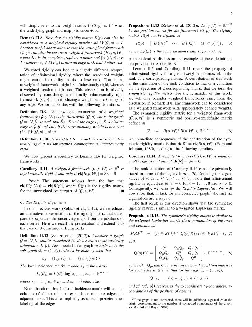
Proposition II.13 (Zelazo et al. (2012)). Let p(V) ∈ Rn×3be the position matrix for the framework (G, p). The rigiditymatrix R(p) can be defined as

R(p) =[El(G1)T · · · El(Gn)T

](In ⊗ p(V)) , (5)

where El(Gi) is the local incidence matrix for node vi.

A more detailed discussion and example of these definitionsare provided in Appendix B.

Lemma II.6 and Corollary II.11 relate the property ofinfinitesimal rigidity for a given (weighted) framework to therank of a corresponding matrix. A contribution of this workis the translation of the rank condition to that of a conditionon the spectrum of a corresponding matrix that we term thesymmetric rigidity matrix. For the remainder of this work,we will only consider weighted frameworks, since from thediscussion in Remark II.8, any framework can be consideredas a weighted framework with appropriately defined weights.

The symmetric rigidity matrix for a weighted framework(G, p,W) is a symmetric and positive-semidefinite matrixdefined as

R := R(p,W)TR(p,W) ∈ R3n×3n. (6)

An immediate consequence of the construction of the sym-metric rigidity matrix is that rk[R] = rk[R(p,W)] (Horn andJohnson, 1985), leading to the following corollary.

Corollary II.14. A weighted framework (G, p,W) is infinites-imally rigid if and only if rk[R] = 3n− 6.

The rank condition of Corollary II.14 can be equivalentlystated in terms of the eigenvalues of R. Denoting the eigen-values of R as λ1 ≤ λ2 ≤ . . . ≤ λ3n, note that infinitesimalrigidity is equivalent to λi = 0 for i = 1, . . . , 6 and λ7 > 0.Consequently, we term λ7 the Rigidity Eigenvalue. We willnow show that, in fact, for any connected graph,2 the first sixeigenvalues are always 0.

The first result in this direction shows that the symmetricrigidity matrix is similar to a weighted Laplacian matrix.

Proposition II.15. The symmetric rigidity matrix is similar tothe weighted Laplacian matrix via a permutation of the rowsand columns as

PRPT = (I3 ⊗ E(G)W )Q(p(V))(I3 ⊗WE(G)T

), (7)

with

Q(p(V)) =

Q2x QxQy QxQz

QyQx Q2y QyQz

QzQx QzQy Q2z

∈ R3m×3m, (8)

where Qx, Qy , and Qz are m×m diagonal weighting matricesfor each edge in G such that for the edge ek = (vi, vj),

[Qs]kk = (psi − psj), s ∈ {x, y, z}and pxi (pyi , pzi ) represents the x-coordinate (y-coordinate, z-coordinate) of the position of agent i.

2If the graph is not connected, there will be additional eigenvalues at theorigin corresponding to the number of connected components of the graph,see (Godsil and Royle, 2001).

6

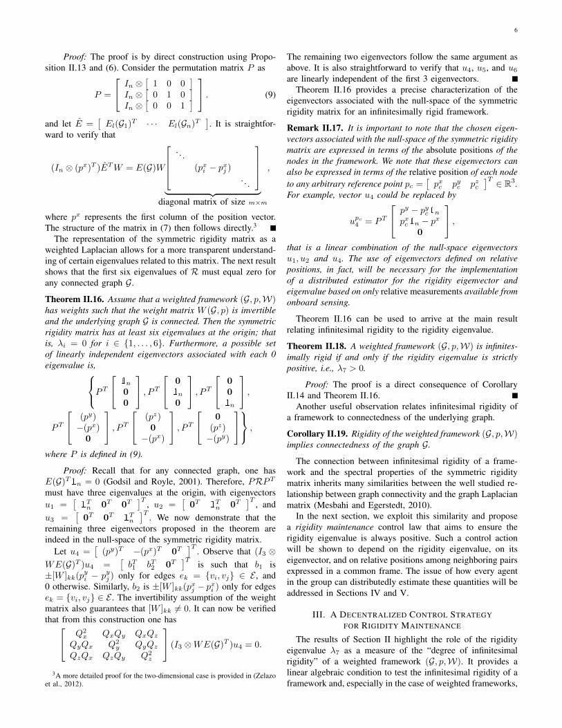
Proof: The proof is by direct construction using Propo-sition II.13 and (6). Consider the permutation matrix P as

P =

In ⊗

[1 0 0

]

In ⊗[

0 1 0]

In ⊗[

0 0 1]

. (9)

and let E =[El(G1)T · · · El(Gn)T

]. It is straightfor-

ward to verify that

(In ⊗ (px)T )ETW = E(G)W

. . .(pxi − pxj )

. . .

︸ ︷︷ ︸diagonal matrix of size m×m

,

where px represents the first column of the position vector.The structure of the matrix in (7) then follows directly.3

The representation of the symmetric rigidity matrix as aweighted Laplacian allows for a more transparent understand-ing of certain eigenvalues related to this matrix. The next resultshows that the first six eigenvalues of R must equal zero forany connected graph G.

Theorem II.16. Assume that a weighted framework (G, p,W)has weights such that the weight matrix W (G, p) is invertibleand the underlying graph G is connected. Then the symmetricrigidity matrix has at least six eigenvalues at the origin; thatis, λi = 0 for i ∈ {1, . . . , 6}. Furthermore, a possible setof linearly independent eigenvectors associated with each 0eigenvalue is,

P

T

1n

00

, PT

01n

0

, PT

001n

,

PT

(py)−(px)0

, PT

(pz)0−(px)

, PT

0(pz)−(py)

,

where P is defined in (9).

Proof: Recall that for any connected graph, one hasE(G)T1n = 0 (Godsil and Royle, 2001). Therefore, PRPTmust have three eigenvalues at the origin, with eigenvectorsu1 =

[1Tn 0T 0T

]T, u2 =

[0T 1

Tn 0T

]T, and

u3 =[0T 0T 1

Tn

]T. We now demonstrate that the

remaining three eigenvectors proposed in the theorem areindeed in the null-space of the symmetric rigidity matrix.

Let u4 =[

(py)T −(px)T 0T]T

. Observe that (I3 ⊗WE(G)T )u4 =

[bT1 bT2 0T

]Tis such that b1 is

±[W ]kk(pyi − pyj ) only for edges ek = {vi, vj} ∈ E , and0 otherwise. Similarly, b2 is ±[W ]kk(pxj − pxi ) only for edgesek = {vi, vj} ∈ E . The invertibility assumption of the weightmatrix also guarantees that [W ]kk 6= 0. It can now be verifiedthat from this construction one has

Q2x QxQy QxQz

QyQx Q2y QyQz

QzQx QzQy Q2z

(I3 ⊗WE(G)T )u4 = 0.

3A more detailed proof for the two-dimensional case is provided in (Zelazoet al., 2012).

The remaining two eigenvectors follow the same argument asabove. It is also straightforward to verify that u4, u5, and u6are linearly independent of the first 3 eigenvectors.

Theorem II.16 provides a precise characterization of theeigenvectors associated with the null-space of the symmetricrigidity matrix for an infinitesimally rigid framework.

Remark II.17. It is important to note that the chosen eigen-vectors associated with the null-space of the symmetric rigiditymatrix are expressed in terms of the absolute positions of thenodes in the framework. We note that these eigenvectors canalso be expressed in terms of the relative position of each nodeto any arbitrary reference point pc =

[pxc pyc pzc

]T ∈ R3.For example, vector u4 could be replaced by

upc4 = PT

py − pyc1npxc1n − px

0

,

that is a linear combination of the null-space eigenvectorsu1, u2 and u4. The use of eigenvectors defined on relativepositions, in fact, will be necessary for the implementationof a distributed estimator for the rigidity eigenvector andeigenvalue based on only relative measurements available fromonboard sensing.

Theorem II.16 can be used to arrive at the main resultrelating infinitesimal rigidity to the rigidity eigenvalue.

Theorem II.18. A weighted framework (G, p,W) is infinites-imally rigid if and only if the rigidity eigenvalue is strictlypositive, i.e., λ7 > 0.

Proof: The proof is a direct consequence of CorollaryII.14 and Theorem II.16.

Another useful observation relates infinitesimal rigidity ofa framework to connectedness of the underlying graph.

Corollary II.19. Rigidity of the weighted framework (G, p,W)implies connectedness of the graph G.

The connection between infinitesimal rigidity of a frame-work and the spectral properties of the symmetric rigiditymatrix inherits many similarities between the well studied re-lationship between graph connectivity and the graph Laplacianmatrix (Mesbahi and Egerstedt, 2010).

In the next section, we exploit this similarity and proposea rigidity maintenance control law that aims to ensure therigidity eigenvalue is always positive. Such a control actionwill be shown to depend on the rigidity eigenvalue, on itseigenvector, and on relative positions among neighboring pairsexpressed in a common frame. The issue of how every agentin the group can distributedly estimate these quantities will beaddressed in Sections IV and V.

III. A DECENTRALIZED CONTROL STRATEGYFOR RIGIDITY MAINTENANCE

The results of Section II highlight the role of the rigidityeigenvalue λ7 as a measure of the “degree of infinitesimalrigidity” of a weighted framework (G, p,W). It provides alinear algebraic condition to test the infinitesimal rigidity of aframework and, especially in the case of weighted frameworks,

7

0 5 10 15 20 25 30 35 40 45 500

20

40

60

80

100

120

140

160

180

200

λ7

Vλ(λ

7)

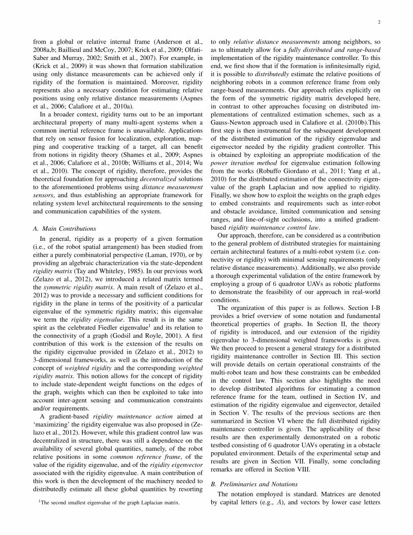
Fig. 2. A possible shape for the rigidity potential function Vλ(λ7) withλmin7 = 5.

provides a means of quantifying “how rigid” a weightedframework is. Moreover, the symmetric rigidity matrix wasshown to have a structure reminiscent of a weighted graphLaplacian matrix, and thus can be considered as a naturallydistributed operator.

The basic approach we consider for the maintenance ofrigidity is to define a scalar potential function of the rigidityeigenvalue, Vλ(λ7) > 0, with the properties of growingunbounded as λ7 → λmin

7 > 0 and vanishing (with vanishingderivative) as λ7 → ∞ (see Fig. 2 for one possible shapeor Vλ with λmin

7 = 5). Here, λmin7 represents some predeter-

mined minimum allowable value for the rigidity eigenvaluedetermined by the needs of the application. In addition tomaintaining rigidity, the potential function should also captureadditional constraints in the system, such as collision avoid-ance or formation maintenance. Each agent should then followthe anti-gradient of this potential function, that is

ξ(u) = pu(t) = − ∂Vλ∂pu(t)

= −∂Vλ∂λ7

∂λ7∂pu(t)

, (10)

where ξ(u) is the velocity input of agent u, as definedin (3), and pu =

[pxu pyu pzu

]Tis the position vector of

the u-th agent. This strategy will ensure that the formationmaintains a “minimum” level of rigidity (i.e., λmin

7 ) at alltimes. Of course, this strategy is an inherently centralizedone, as the computation of the rigidity eigenvalue and ofits gradient require full knowledge of the symmetric rigiditymatrix. Nevertheless, we will proceed with this strategy anddemonstrate that it can be implemented in a fully decentralizedmanner.

In the sequel, we examine in more detail the structure ofthe control scheme (10). First, we show how the formalizationof weighted frameworks allows to embed additional weightswithin the rigidity property that enforce explicit inter-agentsensing and communication constraints and group require-ments such as collision avoidance and formation control. Forinstance, the weighting machinery will be exploited so as toinduce the agents to keep a desired inter-agent distance `0 andto ensure a minimum safety distance `min from neighboringagents and obstacles. With these constraints, the controllerwill simultaneously maintain a minimum level of rigiditywhile also respecting the additional inter-agent constraints.We then provide an explicit characterization of the gradientof the rigidity eigenvalue with respect to the agent positions,and highlight its distributed structure. Finally, we present the

0 1 2 3 4 5 6 70

0.5

1

1.5

ℓuv

γa uv(ℓ

uv)

(a)

0 1 2 3 4 5 6 70

0.5

1

1.5

ℓuvo

γb uv(d

uvo)

(b)

0 1 2 3 4 5 6 7 80

0.5

1

1.5

ℓuv

βuv(ℓ

uv)

(c)

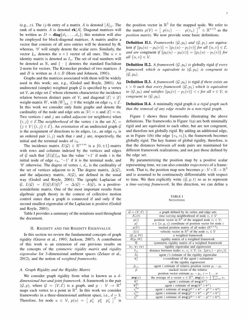
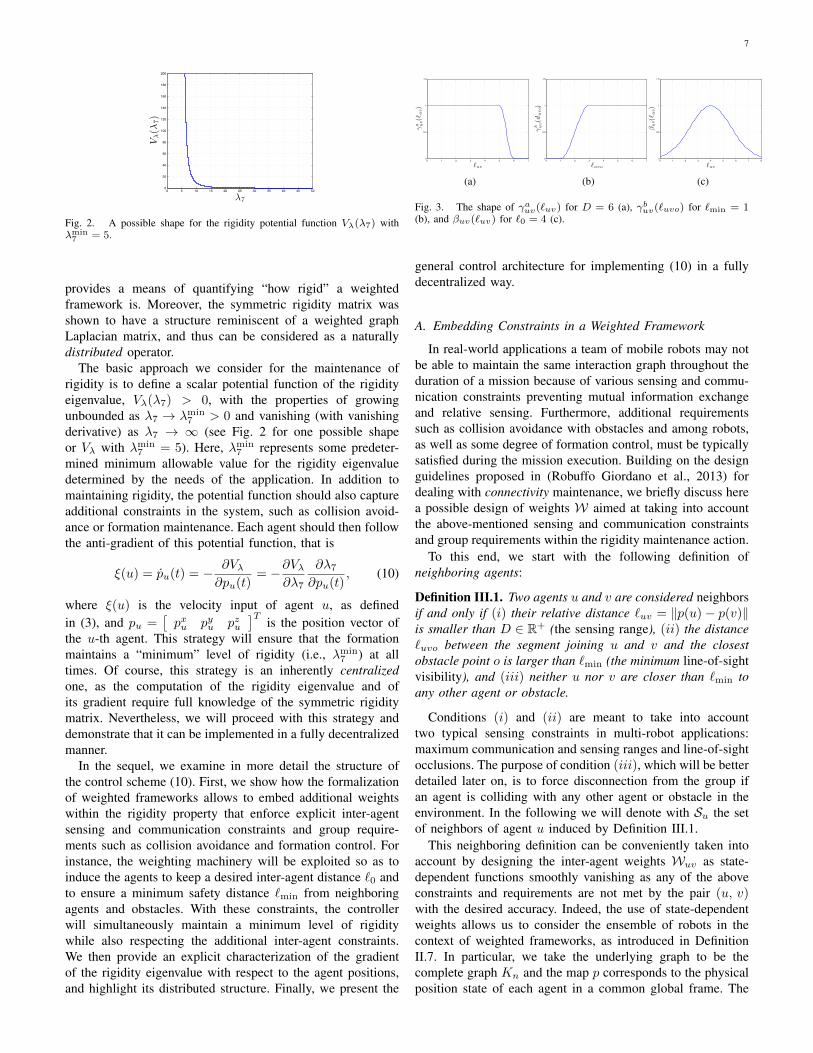
Fig. 3. The shape of γauv(`uv) for D = 6 (a), γbuv(`uvo) for `min = 1(b), and βuv(`uv) for `0 = 4 (c).

general control architecture for implementing (10) in a fullydecentralized way.

A. Embedding Constraints in a Weighted Framework

In real-world applications a team of mobile robots may notbe able to maintain the same interaction graph throughout theduration of a mission because of various sensing and commu-nication constraints preventing mutual information exchangeand relative sensing. Furthermore, additional requirementssuch as collision avoidance with obstacles and among robots,as well as some degree of formation control, must be typicallysatisfied during the mission execution. Building on the designguidelines proposed in (Robuffo Giordano et al., 2013) fordealing with connectivity maintenance, we briefly discuss herea possible design of weights W aimed at taking into accountthe above-mentioned sensing and communication constraintsand group requirements within the rigidity maintenance action.

To this end, we start with the following definition ofneighboring agents:

Definition III.1. Two agents u and v are considered neighborsif and only if (i) their relative distance `uv = ‖p(u)− p(v)‖is smaller than D ∈ R+ (the sensing range), (ii) the distance`uvo between the segment joining u and v and the closestobstacle point o is larger than `min (the minimum line-of-sightvisibility), and (iii) neither u nor v are closer than `min toany other agent or obstacle.

Conditions (i) and (ii) are meant to take into accounttwo typical sensing constraints in multi-robot applications:maximum communication and sensing ranges and line-of-sightocclusions. The purpose of condition (iii), which will be betterdetailed later on, is to force disconnection from the group ifan agent is colliding with any other agent or obstacle in theenvironment. In the following we will denote with Su the setof neighbors of agent u induced by Definition III.1.

This neighboring definition can be conveniently taken intoaccount by designing the inter-agent weights Wuv as state-dependent functions smoothly vanishing as any of the aboveconstraints and requirements are not met by the pair (u, v)with the desired accuracy. Indeed, the use of state-dependentweights allows us to consider the ensemble of robots in thecontext of weighted frameworks, as introduced in DefinitionII.7. In particular, we take the underlying graph to be thecomplete graph Kn and the map p corresponds to the physicalposition state of each agent in a common global frame. The

8

weights are the mapsWuv , and the weighted framework is thetriple (Kn, p,W) with, therefore, Nu = {v ∈ V| Wuv 6= 0}.

Following what was proposed in (Robuffo Giordano et al.,2013), and recalling that `uvo represents the distance betweenthe segment joining agents u and v and the closest obstaclepoint o, we then take

Wuv = αuvβuvγauvγ

buv, (11)

with αuv = αuv(`uk|k∈Su , `vk|k∈Sv ), βuv = βuv(`uv), γauv =γauv(`uv), γbuv = γbuv(`uvo) and such that• – lim`uk→`min

αuv = 0, ∀k ∈ Su,– lim`vk→`min αuv = 0, ∀k ∈ Sv , and– αuv ≡ 0 if `uk ≤ `min or `vk ≤ `min, for anyk ∈ Su, k ∈ Sv;

• lim|`uv−`0|→∞ βuv = 0 with β(`uv) < β(`0)∀ `uv 6= `0;• lim`uv→D γ

auv = 0 with γauv ≡ 0 ∀ `uv ≥ D;

• lim`uvo→`minγbuv = 0 with γbuv ≡ 0 ∀ `uvo ≤ `min.

As explained, `min is a predetermined minimum safety dis-tance for avoiding collisions and line-of-sight occlusions.Figures 3(a)–(c) show an illustrative shape of weights γauv ,γbuv and βuv . The shape of the weights αuv is conceptuallyequivalent to that of weights γbuv in Fig. 3(b).

This weight design results in the following properties: fora given pair of agents (u, v), the weight Wuv will vanish(because of the term γauvγ

buv) whenever the sensing and

communication constraints of Definition III.1 are violated(maximum range, obstacle occlusion), thus resulting in adecreased degree of connectivity of the graph G (edge {u, v}is lost). The same will happen as the inter-distance `uv deviatestoo much from the desired `0 because of the term βuv . Finally,the term αuv will force complete disconnection of vertexes uand v from the other vertexes and therefore a complete loss ofconnectivity for the graph G whenever a collision with anotheragent is approached.4

We now recall from Corollary II.19 that infinitesimal rigid-ity implies graph connectivity. Therefore, any decrease in thedegree of graph connectivity due to the weightsWuv vanishingwill also result in a decrease of rigidity of the weighted frame-work (Kn, p,W) (in particular, rigidity is obviously lost fora disconnected graph). By maintaining λ7 > 0 (in the contextof weighted frameworks) over time, it is then possible topreserve formation rigidity while, at the same time, explicitlyconsidering and managing the above-mentioned sensing andcommunication constraints and requirements.

Remark III.2. We note that the purpose of the weight βuvin (11) is to embed a basic level of formation control into therigidity maintenance action: indeed, every neighboring pairwill try to keep the desired distance `0 thanks to the shape ofthe weights βuv . More complex formation control behaviorscould be obtained by different choices of functions βuv (e.g.,for maintaining given relative positions). Furthermore, forma-tion shapes can be uniquely specified owing to the infinitesimalrigidity property of the configuration.

4As for collision with obstacles, an equivalent behavior is automaticallyobtained from weights γbuv , see again (Robuffo Giordano et al., 2013) for afull explanation. Also note that, because of the definition of weights Wuv ,one has Nu ⊆ Su but Su 6⊂ Nu.

Remark III.3. We further highlight the following propertieswhose explicit proof can be found in (Robuffo Giordano et al.,2013): the chosen weights Wuv are functions of only relativedistances to other agents and obstacles, while their gradientswith respect to the agent position pu (resp. pv) are functionsof relative positions expressed in a common reference frame.Furthermore, Wuv =Wvu and ∂Wuv

∂pu= 0, ∀v /∈ Nu. Finally,

the evaluation of weights Wuv and of their gradients can beperformed in a decentralized way by agent u (reps. v) by onlyresorting to local information and 1-hop communication.

As shown the next developments, these properties willbe instrumental for expressing the gradient of the rigidityeigenvalue as a function of purely relative quantities withrespect to only 1-hop neighbors.

B. The Gradient of the Rigidity Eigenvalue

We now present an explicit characterization of the gradientof the rigidity eigenvalue with respect to the agent positions,as used in the control (10). We first recall that the rigidityeigenvalue can be expressed as

λ7 = vT7Rv7,

where v7 is the normalized rigidity eigenvector associatedwith λ7. For notational convenience, we consider the permutedrigidity eigenvector Pv7 =

[(vx)T (vy)T (vz)T

]T,

where P is defined in Theorem II.16. For the remainder ofthe work, we drop the subscript and reserve the bold fontv for the rigidity eigenvector. Note that in fact, the rigidityeigenvalue and eigenvector are state-dependent, and thereforealso time-varying when the formation is induced by the spatialorientation of a mobile team of robots, or due to the actionof state-dependent weights on the sensing and communicationlinks.

We can now exploit the structure of the symmetric rigid-ity matrix for weighted frameworks. Using the form of thesymmetric rigidity matrix given in (7), we define Q(p(V)) =(I3 ⊗W )Q(p(V))(I3 ⊗W ) as a generalized weight matrix,and observe that

PRPT = (I3 ⊗ E(G)) Q(p(V))(I3 ⊗ E(G)T

).

The elements of Q(p(V)) are entirely in terms of the relativepositions of each agent and the weighting functions definedon the edges as in (11).

The rigidity eigenvalue can now be expressed explicitly as

λ7 =∑

(i, j)∈E

Wij

((p

xi − p

xj )

2(v

xi − v

xj )

2+ (p

yi − p

yj )

2(v

yi − v

yj )

2+

(pzi − p

zj )

2(v

zi − v

zj )

2+ 2(p

xi − p

xj )(p

yi − p

yj )(v

xi − v

xj )(v

yi − v

yj )+

2(pxi − p

xj )(p

zi − p

zj )(v

xi − v

xj )(v

zi − v

zj )+

2 (pyi − p

yj )(p

zi − p

zj )(v

yi − v

yj )(v

zi − v

zj ))

=∑

(i, j)∈E

WijSij .

(12)From (12), one can then derive a closed-form expression for

∂λ7

∂psi, s ∈ {x, y, z}, i.e., the gradient of λ7 with respect to each

agent’s position. In particular, by exploiting the structure ofthe terms Sij and the properties of the employed weights Wij

9

Control

Robot i Position EstimatorEnvironment

...

Rigidity Estimator

...

...

!7

vk, k 2 Ni(t)

vi

pk, k 2 Ni(t)

kpk � pikk 2 Ni(t) pc

i

pck, k 2 Ni(t)

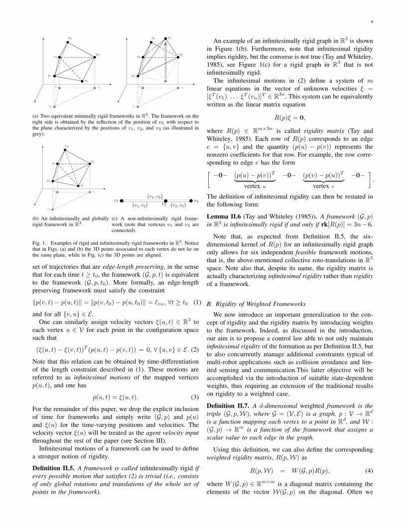
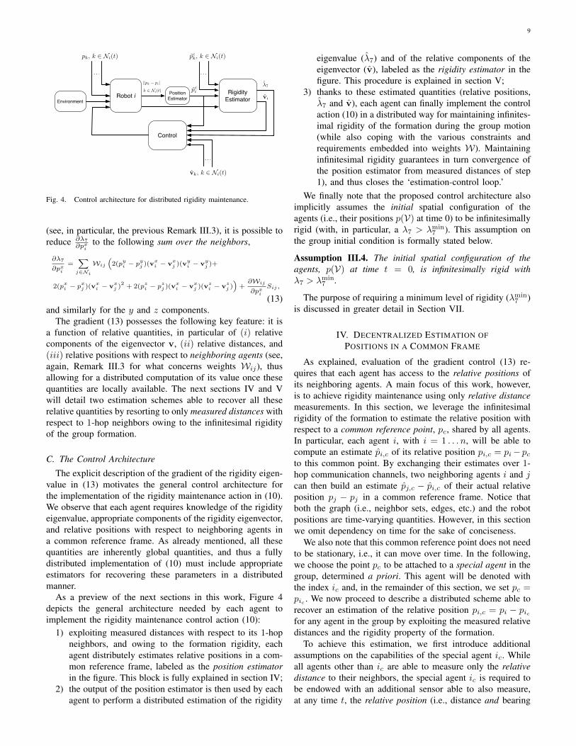
Fig. 4. Control architecture for distributed rigidity maintenance.

(see, in particular, the previous Remark III.3), it is possible toreduce ∂λ7

∂pxito the following sum over the neighbors,

∂λ7

∂pxi=∑

j∈Ni

Wij

(2(p

yi − p

yj )(v

xi − v

xj )(v

yi − v

yj )+

2(pxi − p

xj )(v

xi − v

xj )

2+ 2(p

zi − p

zj )(v

xi − v

xj )(v

zi − v

zj ))+∂Wij

∂pxiSij ,

(13)and similarly for the y and z components.

The gradient (13) possesses the following key feature: it isa function of relative quantities, in particular of (i) relativecomponents of the eigenvector v, (ii) relative distances, and(iii) relative positions with respect to neighboring agents (see,again, Remark III.3 for what concerns weights Wij), thusallowing for a distributed computation of its value once thesequantities are locally available. The next sections IV and Vwill detail two estimation schemes able to recover all theserelative quantities by resorting to only measured distances withrespect to 1-hop neighbors owing to the infinitesimal rigidityof the group formation.

C. The Control Architecture

The explicit description of the gradient of the rigidity eigen-value in (13) motivates the general control architecture forthe implementation of the rigidity maintenance action in (10).We observe that each agent requires knowledge of the rigidityeigenvalue, appropriate components of the rigidity eigenvector,and relative positions with respect to neighboring agents ina common reference frame. As already mentioned, all thesequantities are inherently global quantities, and thus a fullydistributed implementation of (10) must include appropriateestimators for recovering these parameters in a distributedmanner.

As a preview of the next sections in this work, Figure 4depicts the general architecture needed by each agent toimplement the rigidity maintenance control action (10):

1) exploiting measured distances with respect to its 1-hopneighbors, and owing to the formation rigidity, eachagent distributely estimates relative positions in a com-mon reference frame, labeled as the position estimatorin the figure. This block is fully explained in section IV;

2) the output of the position estimator is then used by eachagent to perform a distributed estimation of the rigidity

eigenvalue (λ7) and of the relative components of theeigenvector (v), labeled as the rigidity estimator in thefigure. This procedure is explained in section V;

3) thanks to these estimated quantities (relative positions,λ7 and v), each agent can finally implement the controlaction (10) in a distributed way for maintaining infinites-imal rigidity of the formation during the group motion(while also coping with the various constraints andrequirements embedded into weights W). Maintaininginfinitesimal rigidity guarantees in turn convergence ofthe position estimator from measured distances of step1), and thus closes the ‘estimation-control loop.’

We finally note that the proposed control architecture alsoimplicitly assumes the initial spatial configuration of theagents (i.e., their positions p(V) at time 0) to be infinitesimallyrigid (with, in particular, a λ7 > λmin

7 ). This assumption onthe group initial condition is formally stated below.

Assumption III.4. The initial spatial configuration of theagents, p(V) at time t = 0, is infinitesimally rigid withλ7 > λmin

7 .

The purpose of requiring a minimum level of rigidity (λmin7 )

is discussed in greater detail in Section VII.

IV. DECENTRALIZED ESTIMATION OFPOSITIONS IN A COMMON FRAME

As explained, evaluation of the gradient control (13) re-quires that each agent has access to the relative positions ofits neighboring agents. A main focus of this work, however,is to achieve rigidity maintenance using only relative distancemeasurements. In this section, we leverage the infinitesimalrigidity of the formation to estimate the relative position withrespect to a common reference point, pc, shared by all agents.In particular, each agent i, with i = 1 . . . n, will be able tocompute an estimate pi,c of its relative position pi,c = pi− pcto this common point. By exchanging their estimates over 1-hop communication channels, two neighboring agents i and jcan then build an estimate pj,c − pi,c of their actual relativeposition pj − pj in a common reference frame. Notice thatboth the graph (i.e., neighbor sets, edges, etc.) and the robotpositions are time-varying quantities. However, in this sectionwe omit dependency on time for the sake of conciseness.

We also note that this common reference point does not needto be stationary, i.e., it can move over time. In the following,we choose the point pc to be attached to a special agent in thegroup, determined a priori. This agent will be denoted withthe index ic and, in the remainder of this section, we set pc =pic . We now proceed to describe a distributed scheme able torecover an estimation of the relative position pi,c = pi − picfor any agent in the group by exploiting the measured relativedistances and the rigidity property of the formation.

To achieve this estimation, we first introduce additionalassumptions on the capabilities of the special agent ic. Whileall agents other than ic are able to measure only the relativedistance to their neighbors, the special agent ic is required tobe endowed with an additional sensor able to also measure,at any time t, the relative position (i.e., distance and bearing

10

angles) of at least 2 non-collinear neighbors;5 these two sensedneighbors will be denoted with the indexes (ι(t), κ(t)) ∈Nic(t).

Remark IV.1. We stress that the agent indexes ι(t) and κ(t)are time-varying; indeed, contrarily to the special agent ic,ι(t) and κ(t) are not preassigned to any particular agent inthe multi-robot team. Therefore the special agent ic only needsto measure its relative positions pι(t)−pic and pκ(t)−pic withrespect to any two agents within its neighborhood (ι and κ areeffectively arbitrary), with the points pic , pι(t) and pκ(t) beingnon-collinear ∀t ≥ t0. We believe this assumption is not toorestrictive in practice, as it only require the presence of at leastone robot equipped with a range plus bearing sensor while allthe remaining ones can be equipped with simple range-onlysensors.

In the following we omit for brevity the dependency uponthe time t of the quantities ι and κ.

In order to perform the distributed estimation of pi,c =pi − pc, ∀i ∈ {1, . . . , n} we follow the approach presentedin (Calafiore et al., 2010a), with some slight modificationsdictated by the nature of our problem. Consistently with ournotation, we define p =

[pT1,c . . . pTn,c

]T ∈ R3n. Forcompactness, we also denote by `ij the measured distance‖pj − pi‖, as introduced in Definition III.1. We then considerthe following least squares estimation error:

e(p) =1

4

∑

{i,j}∈E

(‖pj,c − pi,c‖2 − `2ij

)2+

1

2‖pic,c‖2+

+1

2‖pι,c − (pι − pic)‖2 +

1

2‖pκ,c − (pκ − pic)‖2.

(14)

Notice that the quantities `ij , pι − pic , and pκ − pic are mea-sured while all the other quantities represent local estimatesof the robots.

The nonnegative error function e(p) is zero if and only if:• ‖pj,c− pi,c‖ is equal to the measured distance `ij for all

the pairs {i, j} ∈ E ;• ‖pic,c‖ = 0;• pι,c and pκ,c are equal to the measured relative positionspι − pic and pκ − pic , respectively.

Note that the estimates pic,c, pι,c and pκ,c could be directlyset to 0, (pι− pic), and (pι− pic), respectively, since the firstquantity is known and the last two are measured. Nevertheless,we prefer to let the estimator obtaining these values via a‘filtering action’ for the following reasons: first, the estimatorprovides a relatively simple way to filter out noise that mightaffect the relative position measurements; secondly, implemen-tation of the rigidity maintenance controller only requires that(pj,c− pi,c)→ (pj−pi), which is achieved if pj,c → pj− pic,cand pi,c → pi−pic,c for any common value of pic,c. Thereforeany additional hard constraint on pic,c (e.g., pic,c ≡ 0) mightunnecessarily over-constrain the estimator.

Applying a first-order gradient descent method to e(p), wefinally obtain the following decentralized update rule for the

5Formation rigidity implies presence of at least 2 non-collinear neighborsfor each agent (Laman, 1970).

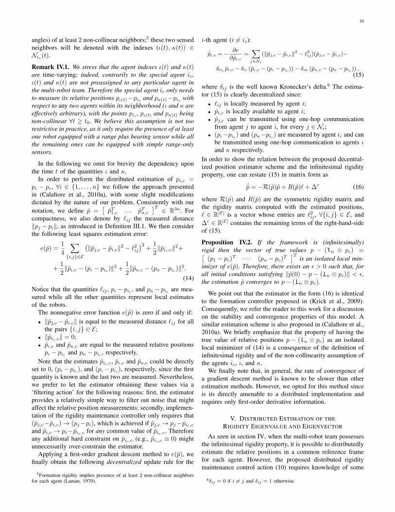
i-th agent (i 6= ic):

˙pi,c = −∂e

∂pi,c=

∑j∈Ni

(‖pj,c − pi,c‖2 − `2ij)(pj,c − pi,c)−

δiic pi,c − δiι (pι,c − (pι − pic))− δiκ (pκ,c − (pκ − pic)) ,(15)

where δij is the well known Kronecker’s delta.6 The estima-tor (15) is clearly decentralized since:• `ij is locally measured by agent i;• pi,c is locally available to agent i;• pj,c can be transmitted using one-hop communication

from agent j to agent i, for every j ∈ Ni;• (pι−pic) and (pκ−pic) are measured by agent ic and can

be transmitted using one-hop communication to agents ιand κ respectively.

In order to show the relation between the proposed decentral-ized position estimator scheme and the infinitesimal rigidityproperty, one can restate (15) in matrix form as

˙p = −R(p)p+R(p)`+ ∆c (16)

where R(p) and R(p) are the symmetric rigidity matrix andthe rigidity matrix computed with the estimated positions,` ∈ R|E| is a vector whose entries are `2ij , ∀{i, j} ∈ E , and∆c ∈ R|E| contains the remaining terms of the right-hand-sideof (15).

Proposition IV.2. If the framework is (infinitesimally)rigid then the vector of true values p − (1n ⊗ pc) =[

(p1 − pc)T · · · (pn − pc)T]T

is an isolated local min-imizer of e(p). Therefore, there exists an ε > 0 such that, forall initial conditions satisfying ‖p(0) − p − (1n ⊗ pc)‖ < ε,the estimation p converges to p− (1n ⊗ pc).

We point out that the estimator in the form (16) is identicalto the formation controller proposed in (Krick et al., 2009).Consequently, we refer the reader to this work for a discussionon the stability and convergence properties of this model. Asimilar estimation scheme is also proposed in (Calafiore et al.,2010a). We briefly emphasize that the property of having thetrue value of relative positions p − (1n ⊗ pc) as an isolatedlocal minimizer of (14) is a consequence of the definition ofinfinitesimal rigidity and of the non-collinearity assumption ofthe agents ic, ι, and κ.

We finally note that, in general, the rate of convergence ofa gradient descent method is known to be slower than otherestimation methods. However, we opted for this method sinceis its directly amenable to a distributed implementation andrequires only first-order derivative information.

V. DISTRIBUTED ESTIMATION OF THERIGIDITY EIGENVALUE AND EIGENVECTOR

As seen in section IV, when the multi-robot team possessesthe infinitesimal rigidity property, it is possible to distributedlyestimate the relative positions in a common reference framefor each agent. However, the proposed distributed rigiditymaintenance control action (10) requires knowledge of some

6δij = 0 if i 6= j and δij = 1 otherwise.

11

additional global quantities that are explicitly expressed inthe expressions (13) and (10). In particular, each agent mustknow also the current value of the rigidity eigenvalue andcertain components of the rigidity eigenvector. In this sec-tion we propose a distributed estimation scheme inspired bythe distributed connectivity maintenance solution proposed in(Yang et al., 2010) for obtaining the rigidity eigenvalue andeigenvector.

For the reader’s convenience, we first provide a briefsummary of the power iteration method for estimating theeigenvalues and eigenvectors of a matrix. We then proceedto show how this estimation process can be distributed byemploying PI consensus filters and by suitably exploiting thestructure of the symmetric rigidity matrix.

A. Power Iteration Method

The power iteration method is one of a suite of iterativealgorithms for estimating the dominant eigenvalue and eigen-vector of a matrix. Following the same procedure as in (Yanget al., 2010), we employ a continuous-time variation of thealgorithm that will compute the smallest non-zero eigenvalueand eigenvector of the symmetric rigidity matrix.

The discrete-time power iteration algorithm is based on thefollowing iteration,

x(k+1) =Ax(k)

‖Ax(k)‖ =Akx(0)

‖Akx(0)‖ .

Under certain assumptions for the matrix A (i.e., no repeatedeigenvalues), the iteration converges to the eigenvector asso-ciated to the largest eigenvalue of the matrix.

To adapt the power iteration to compute the rigidity eigen-vector and eigenvalue, we leverage the results of TheoremII.16 and consider the iteration on a deflated version of thesymmetric rigidity matrix, i.e. R = I − TTT − αR for somesmall enough α > 0. The power iteration method estimates thelargest eigenvalue of a matrix. As all the eigenvalues of thesymmetric rigidity matrix are non-negative, the largest eigen-value of the deflated version R will correspond to 1 − αλ7,and thus can be used to estimate λ7. The constant α ensuresthe matrix R is positive semi-definite.The columns of thematrix T ∈ R3n×6 contain the eigenvectors corresponding tothe zero eigenvalues of R, for example, as characterized inTheorem II.16. Note that the power iteration applied to thematrix R will compute the eigenvector associated with therigidity eigenvalue.7

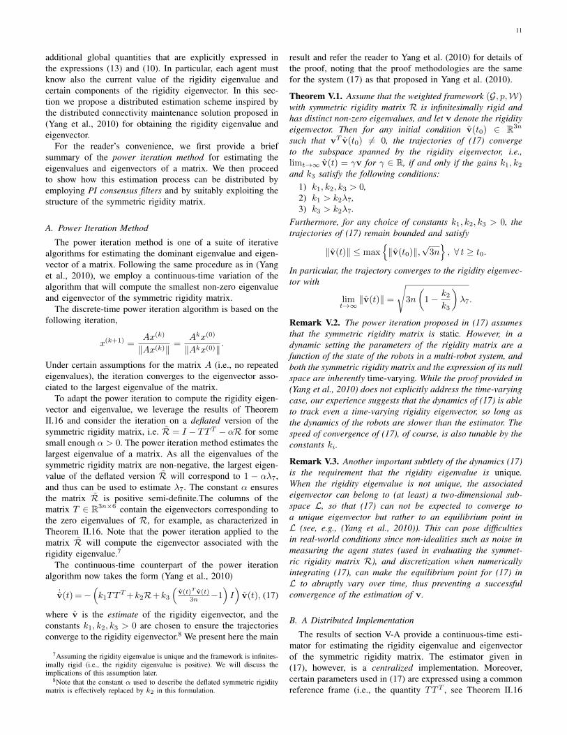
The continuous-time counterpart of the power iterationalgorithm now takes the form (Yang et al., 2010)

˙v(t) =−(k1TT

T+k2R+k3

(v(t)T v(t)

3n −1)I)v(t), (17)

where v is the estimate of the rigidity eigenvector, and theconstants k1, k2, k3 > 0 are chosen to ensure the trajectoriesconverge to the rigidity eigenvector.8 We present here the main

7Assuming the rigidity eigenvalue is unique and the framework is infinites-imally rigid (i.e., the rigidity eigenvalue is positive). We will discuss theimplications of this assumption later.

8Note that the constant α used to describe the deflated symmetric rigiditymatrix is effectively replaced by k2 in this formulation.

result and refer the reader to Yang et al. (2010) for details ofthe proof, noting that the proof methodologies are the samefor the system (17) as that proposed in Yang et al. (2010).

Theorem V.1. Assume that the weighted framework (G, p,W)with symmetric rigidity matrix R is infinitesimally rigid andhas distinct non-zero eigenvalues, and let v denote the rigidityeigenvector. Then for any initial condition v(t0) ∈ R3n

such that vT v(t0) 6= 0, the trajectories of (17) convergeto the subspace spanned by the rigidity eigenvector, i.e.,limt→∞ v(t) = γv for γ ∈ R, if and only if the gains k1, k2and k3 satisfy the following conditions:

1) k1, k2, k3 > 0,2) k1 > k2λ7,3) k3 > k2λ7.

Furthermore, for any choice of constants k1, k2, k3 > 0, thetrajectories of (17) remain bounded and satisfy

‖v(t)‖ ≤ max{‖v(t0)‖,

√3n}, ∀ t ≥ t0.

In particular, the trajectory converges to the rigidity eigenvec-tor with

limt→∞

‖v(t)‖ =

√3n

(1− k2

k3

)λ7.

Remark V.2. The power iteration proposed in (17) assumesthat the symmetric rigidity matrix is static. However, in adynamic setting the parameters of the rigidity matrix are afunction of the state of the robots in a multi-robot system, andboth the symmetric rigidity matrix and the expression of its nullspace are inherently time-varying. While the proof provided in(Yang et al., 2010) does not explicitly address the time-varyingcase, our experience suggests that the dynamics of (17) is ableto track even a time-varying rigidity eigenvector, so long asthe dynamics of the robots are slower than the estimator. Thespeed of convergence of (17), of course, is also tunable by theconstants ki.

Remark V.3. Another important subtlety of the dynamics (17)is the requirement that the rigidity eigenvalue is unique.When the rigidity eigenvalue is not unique, the associatedeigenvector can belong to (at least) a two-dimensional sub-space L, so that (17) can not be expected to converge toa unique eigenvector but rather to an equilibrium point inL (see, e.g., (Yang et al., 2010)). This can pose difficultiesin real-world conditions since non-idealities such as noise inmeasuring the agent states (used in evaluating the symmet-ric rigidity matrix R), and discretization when numericallyintegrating (17), can make the equilibrium point for (17) inL to abruptly vary over time, thus preventing a successfulconvergence of the estimation of v.

B. A Distributed Implementation

The results of section V-A provide a continuous-time esti-mator for estimating the rigidity eigenvalue and eigenvectorof the symmetric rigidity matrix. The estimator given in(17), however, is a centralized implementation. Moreover,certain parameters used in (17) are expressed using a commonreference frame (i.e., the quantity TTT , see Theorem II.16

12

and Remark II.17) or require each robot to know the entireestimator state (i.e., the quantity v(t)T v(t) in (17)). Wepropose in this sub-section a distributed implementation forthe rigidity estimator that overcomes these difficulties, inparticular by leveraging the results of Section IV. In the samespirit as the solution proposed in (Yang et al., 2010), we makeuse of the PI average consensus filter (Freeman et al., 2006)to distributedly compute the necessary quantities of interest,and strongly exploit the particular structure of the symmetricrigidity matrix.

Our approach to the distribution of (17) is to exploit both thebuilt-in distributed structure (i.e., the symmetric rigidity matrixR) and the reduction of the other parameters to values that allagents can obtain via a distributed algorithm. In this direction,we now proceed to analyze each term in (17) and discussthe appropriate strategies for implementing the estimator in adistributed fashion.

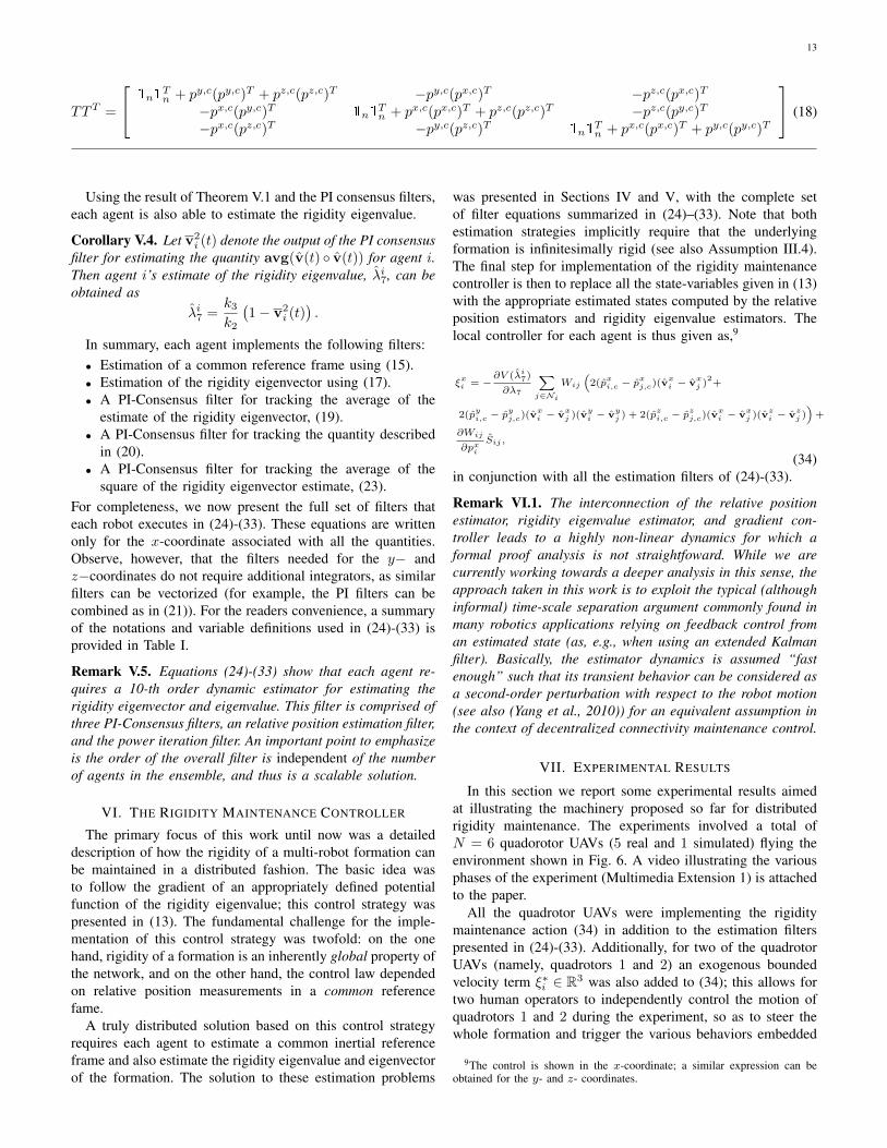
Concerning the first term TTT v, Theorem II.16 provides ananalytic characterization of the eigenvectors associated withthe zero eigenvalues of the symmetric rigidity matrix (assum-ing the graph is infinitesimally rigid). To begin the analysis,we explicitly write out the matrix T and examine the elementsof the matrix TTT . Following the comments of RemarkII.17, we express the null-space vectors in terms of relativepositions to an arbitrary point pc=

[pxc pyc pzc

]∈ R3; in

particular, the point pc will be the special agent ic describedin Section IV.

T =

1n 0 0 py − pyc1n pz − pzc1n 00 1n 0 pxc1n − px 0 pz − pzc1n0 0 1n 0 pxc1n − px pyc1n − py

For the remainder of this discussion, we assume that all agentshave access to their state in an estimated coordinate framerelative to the point pic , the details of which were describedin Section IV.

To simplify notations, we write as in Section IV, for exam-ple, py,c = py−pyc1n, and pi,c = pi−pc. Following our earliernotation, we also partition the vector v into each coordinate,vx, vy , and vz . Let avg(r) denote the average value of theelements in the vector r ∈ Rn, i.e. avg(r) = 1

n1Tn r. Then it

is straightforward to verify that

1n1Tn v

k(t) = navg(vk(t))1n, k ∈ {x, y, z} (19)

pi,c(pj,c)T vk(t) = navg(pj,c ◦ vk)pi,c, i, j, k ∈ {x, y, z},

(20)

where ‘◦’ denotes the element-wise multiplication of twovectors.

This characterization highlights that, in order to evaluate theterm TTT v, each agent must compute the average amongst allagents of a certain value that is a function of the current state ofthe estimator and of the positions in some common referenceframe whose origin is the point pc. It is well known that theconsensus protocol can be used to distributedly compute theaverage of a set of numbers (Mesbahi and Egerstedt, 2010).The speed at which the consensus protocol can compute thisvalue is a function of the connectivity of the underlying graphand the weights used in the protocol. In this framework,

PI Consensus

Filter

PI Consensus

Filter

PI Consensus

Filter

G(t)

�px(t)

�py(t)

�pz(t)

vz(t)

vx(t)

vy(t)

X

X

X

⇥I 0 0

⇤TTT

24

vx(t)vy(t)vz(t)

35

n

n

n

Fig. 5. Block diagram showing PI consensus filters in calculation ofTTT v(t).

however, a direct application of the consensus protocol willnot be sufficient. Indeed, it is expected that each agent will bephysically moving, leading to a time-varying description of thematrix TTT (see Remark V.2). Additionally, the underlyingnetwork is also dynamic as sensing links between agents areinherently state dependent.

The use of a dynamic consensus protocol introduces ad-ditional tuning parameters that can be used to ensure thatthe distributed average calculation converges faster than theunderlying dynamics of each agent in the system, as well asthe ability to track the average of a time-varying signal. Weemploy the following PI average consensus filter proposed in(Freeman et al., 2006),

[z(t)w(t)

]=

[−γIn −KPL(G(t)) KIL(G(t))−KIL(G(t)) 0

] [z(t)w(t)

]

+

[γIn0

]u(t) (21)

y(t) =[In 0

] [ z(t)w(t)

]. (22)

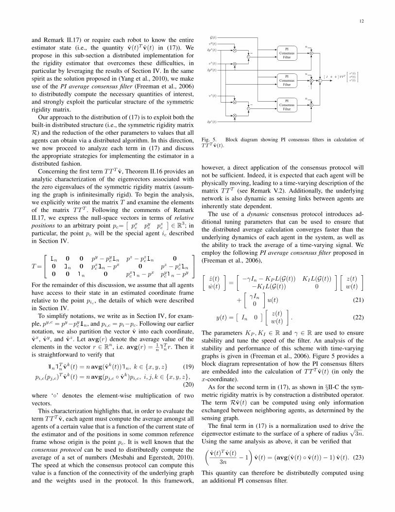
The parameters KP ,KI ∈ R and γ ∈ R are used to ensurestability and tune the speed of the filter. An analysis of thestability and performance of this scheme with time-varyinggraphs is given in (Freeman et al., 2006). Figure 5 provides ablock diagram representation of how the PI consensus filtersare embedded into the calculation of TTT v(t) (in only thex-coordinate).

As for the second term in (17), as shown in §II-C the sym-metric rigidity matrix is by construction a distributed operator.The term Rv(t) can be computed using only informationexchanged between neighboring agents, as determined by thesensing graph.

The final term in (17) is a normalization used to drive theeigenvector estimate to the surface of a sphere of radius

√3n.

Using the same analysis as above, it can be verified that(v(t)T v(t)

3n− 1

)v(t) = (avg(v(t) ◦ v(t))− 1) v(t). (23)

This quantity can therefore be distributedly computed usingan additional PI consensus filter.

13

TTT =

1n1

Tn + py,c(py,c)T + pz,c(pz,c)T −py,c(px,c)T −pz,c(px,c)T

−px,c(py,c)T 1n1Tn + px,c(px,c)T + pz,c(pz,c)T −pz,c(py,c)T

−px,c(pz,c)T −py,c(pz,c)T 1n1Tn + px,c(px,c)T + py,c(py,c)T

(18)

Using the result of Theorem V.1 and the PI consensus filters,each agent is also able to estimate the rigidity eigenvalue.

Corollary V.4. Let v2i (t) denote the output of the PI consensus

filter for estimating the quantity avg(v(t) ◦ v(t)) for agent i.Then agent i’s estimate of the rigidity eigenvalue, λi7, can beobtained as

λi7 =k3k2

(1− v2

i (t)).

In summary, each agent implements the following filters:• Estimation of a common reference frame using (15).• Estimation of the rigidity eigenvector using (17).• A PI-Consensus filter for tracking the average of the

estimate of the rigidity eigenvector, (19).• A PI-Consensus filter for tracking the quantity described

in (20).• A PI-Consensus filter for tracking the average of the

square of the rigidity eigenvector estimate, (23).For completeness, we now present the full set of filters thateach robot executes in (24)-(33). These equations are writtenonly for the x-coordinate associated with all the quantities.Observe, however, that the filters needed for the y− andz−coordinates do not require additional integrators, as similarfilters can be vectorized (for example, the PI filters can becombined as in (21)). For the readers convenience, a summaryof the notations and variable definitions used in (24)-(33) isprovided in Table I.

Remark V.5. Equations (24)-(33) show that each agent re-quires a 10-th order dynamic estimator for estimating therigidity eigenvector and eigenvalue. This filter is comprised ofthree PI-Consensus filters, an relative position estimation filter,and the power iteration filter. An important point to emphasizeis the order of the overall filter is independent of the numberof agents in the ensemble, and thus is a scalable solution.

VI. THE RIGIDITY MAINTENANCE CONTROLLER

The primary focus of this work until now was a detaileddescription of how the rigidity of a multi-robot formation canbe maintained in a distributed fashion. The basic idea wasto follow the gradient of an appropriately defined potentialfunction of the rigidity eigenvalue; this control strategy waspresented in (13). The fundamental challenge for the imple-mentation of this control strategy was twofold: on the onehand, rigidity of a formation is an inherently global property ofthe network, and on the other hand, the control law dependedon relative position measurements in a common referencefame.

A truly distributed solution based on this control strategyrequires each agent to estimate a common inertial referenceframe and also estimate the rigidity eigenvalue and eigenvectorof the formation. The solution to these estimation problems

was presented in Sections IV and V, with the complete setof filter equations summarized in (24)–(33). Note that bothestimation strategies implicitly require that the underlyingformation is infinitesimally rigid (see also Assumption III.4).The final step for implementation of the rigidity maintenancecontroller is then to replace all the state-variables given in (13)with the appropriate estimated states computed by the relativeposition estimators and rigidity eigenvalue estimators. Thelocal controller for each agent is thus given as,9

ξxi = −

∂V (λi7)

∂λ7

∑j∈Ni

Wij

(2(p

xi,c − p

xj,c)(v

xi − v

xj )

2+

2(pyi,c − p

yj,c)(v

xi − v

xj )(v

yi − v

yj ) + 2(p

zi,c − p

zj,c)(v

xi − v

xj )(v

zi − v

zj ))+

∂Wij

∂pxiSij ,

(34)in conjunction with all the estimation filters of (24)-(33).

Remark VI.1. The interconnection of the relative positionestimator, rigidity eigenvalue estimator, and gradient con-troller leads to a highly non-linear dynamics for which aformal proof analysis is not straightfoward. While we arecurrently working towards a deeper analysis in this sense, theapproach taken in this work is to exploit the typical (althoughinformal) time-scale separation argument commonly found inmany robotics applications relying on feedback control froman estimated state (as, e.g., when using an extended Kalmanfilter). Basically, the estimator dynamics is assumed “fastenough” such that its transient behavior can be considered asa second-order perturbation with respect to the robot motion(see also (Yang et al., 2010)) for an equivalent assumption inthe context of decentralized connectivity maintenance control.

VII. EXPERIMENTAL RESULTS

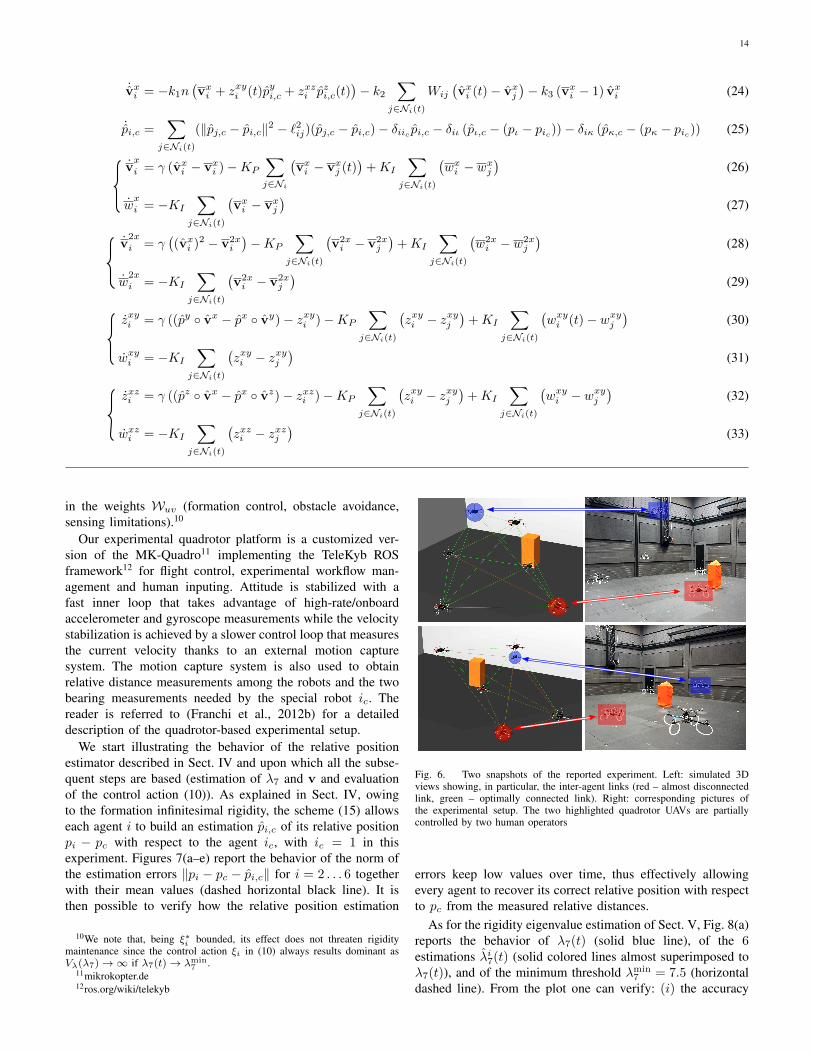
In this section we report some experimental results aimedat illustrating the machinery proposed so far for distributedrigidity maintenance. The experiments involved a total ofN = 6 quadorotor UAVs (5 real and 1 simulated) flying theenvironment shown in Fig. 6. A video illustrating the variousphases of the experiment (Multimedia Extension 1) is attachedto the paper.

All the quadrotor UAVs were implementing the rigiditymaintenance action (34) in addition to the estimation filterspresented in (24)-(33). Additionally, for two of the quadrotorUAVs (namely, quadrotors 1 and 2) an exogenous boundedvelocity term ξ∗i ∈ R3 was also added to (34); this allows fortwo human operators to independently control the motion ofquadrotors 1 and 2 during the experiment, so as to steer thewhole formation and trigger the various behaviors embedded

9The control is shown in the x-coordinate; a similar expression can beobtained for the y- and z- coordinates.

14

˙vxi = −k1n(vxi + zxyi (t)pyi,c + zxzi pzi,c(t)

)− k2

∑

j∈Ni(t)

Wij

(vxi (t)− vxj

)− k3 (vxi − 1) vxi (24)

˙pi,c =∑

j∈Ni(t)

(‖pj,c − pi,c‖2 − `2ij)(pj,c − pi,c)− δiic pi,c − δiι (pι,c − (pι − pic))− δiκ (pκ,c − (pκ − pic)) (25)

vx

i = γ (vxi − vxi )−KP

∑

j∈Ni

(vxi − vxj (t)

)+KI

∑

j∈Ni(t)

(wxi − wxj

)(26)

wxi = −KI

∑

j∈Ni(t)

(vxi − vxj

)(27)

v2x

i = γ((vxi )2 − v2x

i

)−KP

∑

j∈Ni(t)

(v2xi − v2x

j

)+KI

∑

j∈Ni(t)

(w2xi − w2x

j

)(28)

w2xi = −KI

∑

j∈Ni(t)

(v2xi − v2x

j

)(29)

zxyi = γ ((py ◦ vx − px ◦ vy)− zxyi )−KP

∑

j∈Ni(t)

(zxyi − zxyj

)+KI

∑

j∈Ni(t)

(wxyi (t)− wxyj

)(30)

wxyi = −KI

∑

j∈Ni(t)

(zxyi − zxyj

)(31)

zxzi = γ ((pz ◦ vx − px ◦ vz)− zxzi )−KP

∑

j∈Ni(t)

(zxyi − zxyj

)+KI

∑

j∈Ni(t)

(wxyi − wxyj

)(32)

wxzi = −KI

∑

j∈Ni(t)

(zxzi − zxzj

)(33)

in the weights Wuv (formation control, obstacle avoidance,sensing limitations).10

Our experimental quadrotor platform is a customized ver-sion of the MK-Quadro11 implementing the TeleKyb ROSframework12 for flight control, experimental workflow man-agement and human inputing. Attitude is stabilized with afast inner loop that takes advantage of high-rate/onboardaccelerometer and gyroscope measurements while the velocitystabilization is achieved by a slower control loop that measuresthe current velocity thanks to an external motion capturesystem. The motion capture system is also used to obtainrelative distance measurements among the robots and the twobearing measurements needed by the special robot ic. Thereader is referred to (Franchi et al., 2012b) for a detaileddescription of the quadrotor-based experimental setup.

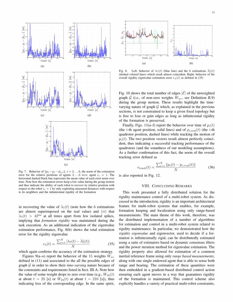
We start illustrating the behavior of the relative positionestimator described in Sect. IV and upon which all the subse-quent steps are based (estimation of λ7 and v and evaluationof the control action (10)). As explained in Sect. IV, owingto the formation infinitesimal rigidity, the scheme (15) allowseach agent i to build an estimation pi,c of its relative positionpi − pc with respect to the agent ic, with ic = 1 in thisexperiment. Figures 7(a–e) report the behavior of the norm ofthe estimation errors ‖pi − pc − pi,c‖ for i = 2 . . . 6 togetherwith their mean values (dashed horizontal black line). It isthen possible to verify how the relative position estimation

10We note that, being ξ∗i bounded, its effect does not threaten rigiditymaintenance since the control action ξi in (10) always results dominant asVλ(λ7)→∞ if λ7(t)→ λmin

7 .11mikrokopter.de12ros.org/wiki/telekyb

Fig. 6. Two snapshots of the reported experiment. Left: simulated 3Dviews showing, in particular, the inter-agent links (red – almost disconnectedlink, green – optimally connected link). Right: corresponding pictures ofthe experimental setup. The two highlighted quadrotor UAVs are partiallycontrolled by two human operators

errors keep low values over time, thus effectively allowingevery agent to recover its correct relative position with respectto pc from the measured relative distances.

As for the rigidity eigenvalue estimation of Sect. V, Fig. 8(a)reports the behavior of λ7(t) (solid blue line), of the 6estimations λi7(t) (solid colored lines almost superimposed toλ7(t)), and of the minimum threshold λmin

7 = 7.5 (horizontaldashed line). From the plot one can verify: (i) the accuracy

15

0 50 100 150 200 250 3000

0.05

0.1

0.15

0.2

0.25

time [s]

‖p2−

pc−

p2,c‖[m

]

(a)

0 50 100 150 200 250 3000

0.02

0.04

0.06

0.08

0.1

0.12

0.14

0.16

0.18

0.2

time [s]

‖p3−

pc−

p3,c‖[m

]

(b)

0 50 100 150 200 250 3000

0.05

0.1

0.15

0.2

0.25

time [s]

‖p4−

pc−

p4,c‖[m

]

(c)

0 50 100 150 200 250 3000

0.05

0.1

0.15

0.2

0.25

0.3

0.35

time [s]

‖p5−

pc−

p5,c‖[m

]

(d)

0 50 100 150 200 250 3000

0.05

0.1

0.15

0.2

0.25

0.3

0.35

time [s]

‖p6−

pc−

p6,c‖[m

]

(e)

Fig. 7. Behavior of ‖pi−pc− pi,c‖, i = 2 . . . 6, the norm of the estimationerror for the relative positions of agents 2 . . . 6 w.r.t. agent ic = 1. Thehorizontal dashed black line represents the mean value of each error norm overtime. Note how the estimation errors keep a low value during the group motionand thus indicate the ability of each robot to recover its relative position withrespect to the robot ic = 1 by only exploiting measured distances with respectto its neighbors and the infinitesimal rigidity of the formation

in recovering the value of λ7(t) (note how the 6 estimationsare almost superimposed on the real value) and (ii) thatλ7(t) > λmin

7 at all times apart from few isolated spikes,implying that formation rigidity was maintained during thetask execution. As an additional indication of the eigenvalueestimation performance, Fig. 8(b) shows the total estimationerror for the rigidity eigenvalue

eλ(t) =

∑Ni=1 |λ7(t)− λi7(t)|

N(35)

which again confirms the accuracy of the estimation strategy.Figures 9(a–o) report the behavior of the 15 weights Wuv

defined in (11) and associated to the all the possible edges ofgraph G in order to show their time-varying nature because ofthe constraints and requirements listed in Sect. III-A. Note howthe value of some weight drops to zero over time (e.g., W45(t)at about t = 25 [s] or W24(t) at about t = 210 [s]), thusindicating loss of the corresponding edge. In the same spirit,

0 50 100 150 200 250 3004

5

6

7

8

9

10

11

12

13

14

time [s]

λ7,λi 7,

λ8

(a)

0 50 100 150 200 250 3000

0.5

1

1.5

2

2.5

3

3.5

4

4.5

5

time [s]

eλ7

(b)

Fig. 8. Left: behavior of λ7(t) (blue line) and the 6 estimations λi7(t)(dashed colored lines) which result almost coincident. Right: behavior of theoverall rigidity eigenvalue estimation error eλ(t) as defined in (35)

Fig. 10 shows the total number of edges |E | of the unweightedgraph G (i.e., of non-zero weights Wuv , see Definition II.9)during the group motion. These results highlight the time-varying nature of graph G which, as explained in the previoussections, is not constrained to keep a given fixed topology butis free to lose or gain edges as long as infinitesimal rigidityof the formation is preserved.

Finally, Figs. 11(a–f) report the behavior over time of pi(t)(the i-th agent position, solid lines) and of pi,real(t) (the i-thquadrotor position, dashed lines) while tracking the motion ofpi(t). The two position vectors result almost perfectly coinci-dent, thus indicating a successful tracking performance of thequadrotors (and the soundness of our modeling assumptions).As a further confirmation of this fact, the norm of the overalltracking error defined as

etrack(t) =

∑Ni=1 ‖pi(t)− pi,real(t)‖

N(36)

is also reported in Fig. 12.

VIII. CONCLUDING REMARKS

This work presented a fully distributed solution for therigidity maintenance control of a multi-robot system. As dis-cussed in the introduction, rigidity is an important architecturalfeature for multi-robot systems that enables, for example,formation keeping and localization using only range-basedmeasurements. The main theme of this work, therefore, wasthe distributed implementation of a number of algorithmsfor estimation and control in a multi-robot system related torigidity maintenance. In particular, we demonstrated how therigidity eigenvalue and eigenvector, used to decide if a for-mation is infinitesimally rigid, can be distributedly estimatedusing a suite of estimators based on dynamic consensus filtersand the power iteration method for eigenvalue estimation. Therigidity property also allowed for estimation of a commoninertial reference frame using only range based measurements,along with one single endowed agent that is able to sense bothrange and bearing. The estimation of these quantities werethen embedded in a gradient-based distributed control actionensuring each agent moves in a way that guarantees rigidityof the formation is maintained. This control scheme alsoexplicitly handles a variety of practical multi-robot constraints,

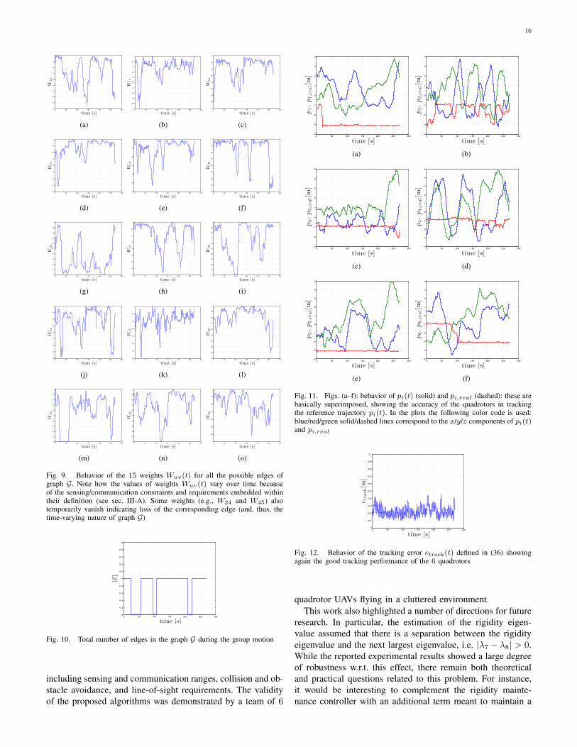
16

0 50 100 150 200 250 3000.1

0.2

0.3

0.4

0.5

0.6

0.7

0.8

0.9

1

time [s]

W12

(a)

0 50 100 150 200 250 3000.5

0.55

0.6

0.65

0.7

0.75

0.8

0.85

0.9

0.95

1

time [s]

W13

(b)

0 50 100 150 200 250 3000.2

0.3

0.4

0.5

0.6

0.7

0.8

0.9

1

time [s]

W14

(c)

0 50 100 150 200 250 3000.2

0.3

0.4

0.5

0.6

0.7

0.8

0.9

1

time [s]

W15

(d)

0 50 100 150 200 250 3000.4

0.5

0.6

0.7

0.8

0.9

1

time [s]

W16

(e)

0 50 100 150 200 250 3000.2

0.3

0.4

0.5

0.6

0.7

0.8

0.9

1

time [s]

W23

(f)

0 50 100 150 200 250 3000

0.1

0.2

0.3

0.4

0.5

0.6

0.7

0.8

0.9

1

time [s]

W24

(g)

0 50 100 150 200 250 3000.2

0.3

0.4

0.5

0.6

0.7

0.8

0.9

1

time [s]

W25

(h)

0 50 100 150 200 250 3000

0.1

0.2

0.3

0.4

0.5

0.6

0.7

0.8

0.9

1

time [s]

W26

(i)

0 50 100 150 200 250 3000.2

0.3

0.4

0.5

0.6

0.7

0.8

0.9

1

time [s]

W34

(j)

0 50 100 150 200 250 3000.65

0.7

0.75

0.8

0.85

0.9

0.95

1

time [s]

W35

(k)

0 50 100 150 200 250 3000.1

0.2

0.3

0.4

0.5

0.6

0.7

0.8

0.9

1

time [s]

W36

(l)

0 50 100 150 200 250 3000

0.1

0.2

0.3

0.4

0.5

0.6

0.7

0.8

0.9

1

time [s]

W45

(m)

0 50 100 150 200 250 3000

0.1

0.2

0.3

0.4

0.5

0.6

0.7

0.8

0.9

1

time [s]

W46

(n)

0 50 100 150 200 250 300

0.4

0.5

0.6

0.7

0.8

0.9

1

time [s]

W56

(o)

Fig. 9. Behavior of the 15 weights Wuv(t) for all the possible edges ofgraph G. Note how the values of weights Wuv(t) vary over time becauseof the sensing/communication constraints and requirements embedded withintheir definition (see sec. III-A). Some weights (e.g., W24 and W45) alsotemporarily vanish indicating loss of the corresponding edge (and, thus, thetime-varying nature of graph G)

0 50 100 150 200 250 30014

14.2

14.4

14.6

14.8

15

15.2

15.4

15.6

15.8

16

time [s]

|E|

Fig. 10. Total number of edges in the graph G during the group motion

including sensing and communication ranges, collision and ob-stacle avoidance, and line-of-sight requirements. The validityof the proposed algorithms was demonstrated by a team of 6

0 50 100 150 200 250 300−4

−3

−2

−1

0

1

2

3

4

time [s]

p1,p1,real[m]

(a)

0 50 100 150 200 250 300−4

−3

−2

−1

0

1

2

3

4

time [s]

p2,p2,real[m]

(b)

0 50 100 150 200 250 300−3

−2

−1

0

1

2

3

4

5

time [s]

p3,p3,real[m]

(c)

0 50 100 150 200 250 300−4

−3

−2

−1

0

1

2

3

4

5

time [s]

p4,p4,real[m]

(d)

0 50 100 150 200 250 300−4

−3

−2

−1

0

1

2

3

4

5

time [s]

p5,p5,real[m]

(e)

0 50 100 150 200 250 300−5

−4

−3

−2

−1

0

1

2

3

4

time [s]

p6,p6,real[m]

(f)

Fig. 11. Figs. (a–f): behavior of pi(t) (solid) and pi,real (dashed): these arebasically superimposed, showing the accuracy of the quadrotors in trackingthe reference trajectory pi(t). In the plots the following color code is used:blue/red/green solid/dashed lines correspond to the x/y/z components of pi(t)and pi,real

0 50 100 150 200 250 3000

0.01

0.02

0.03

0.04

0.05

0.06

0.07

0.08

0.09

0.1

time [s]

etrack[m

]

Fig. 12. Behavior of the tracking error etrack(t) defined in (36) showingagain the good tracking performance of the 6 quadrotors

quadrotor UAVs flying in a cluttered environment.This work also highlighted a number of directions for future

research. In particular, the estimation of the rigidity eigen-value assumed that there is a separation between the rigidityeigenvalue and the next largest eigenvalue, i.e. |λ7 − λ8| > 0.While the reported experimental results showed a large degreeof robustness w.r.t. this effect, there remain both theoreticaland practical questions related to this problem. For instance,it would be interesting to complement the rigidity mainte-nance controller with an additional term meant to maintain a

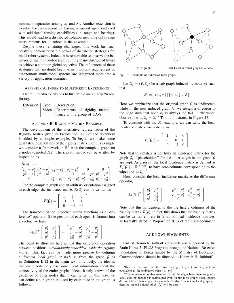
17

minimum separation among λ8 and λ7. Another extension isto relax the requirement for having a special agent endowedwith additional sensing capabilities (i.e. range and bearing).This would lead to a distributed solution involving only rangemeasurements for all robots in the ensemble.

Despite these remaining challenges, this work has suc-cessfully demonstrated the power of distributed strategies formulti-robot systems. Indeed, it is remarkable to observe the be-havior of the multi-robot team running many distributed filtersto achieve a common global objective. The refinement of thesestrategies will no doubt become an important requirement asautonomous multi-robot systems are integrated more into avariety of application domains.

APPENDIX A: INDEX TO MULTIMEDIA EXTENSIONS

The multimedia extensions to this article are at: http://www.ijrr.org.

Extension Type Description1 Video Experiments of rigidity mainte-

nance with a group of UAVs

APPENDIX B: RIGIDITY MATRIX EXAMPLE

The development of the alternative representation of theRigidity Matrix given in Proposition II.13 of the documentis aided by a simple example. To begin, we make somequalitative observations of the rigidity matrix. For this examplewe consider a framework in R2 with the complete graph on3 nodes (denoted K3). The rigidity matrix can be written byinspection as

R(p) =px1 − px2 py1 − py2 px2 − px1 py2 − py1 0 0px1 − px3 py1 − py3 0 0 px3 − px1 py3 − py1

0 0 px2 − px3 py2 − py3 px3 − px2 py3 − py2

.

For the complete graph and an arbitrary orientation assignedto each edge, the incidence matrix E(G) can be written as

E(G) =

1 1 0−1 0 10 −1 −1

.

The transpose of the incidence matrix functions as a “dif-ference” operator. If the position of each agent is formed intoa vector, we have

E(G)T

px1 py1px2 py2px3 py3

=

px1 − px2 py1 − py2px1 − px3 py1 − py3px2 − px3 py2 − py3

.

The point to illustrate here is that this difference operationbetween positions is redundantly embedded inside the rigiditymatrix. This fact can be made more precise by defininga directed local graph at node vi from the graph G asin Definition II.12 in the main text. Intuitively, the idea isthat each node only has some local information about theconnectivity of the entire graph; indeed, it only knows of theexistence of other nodes that it can sense. In this way, wecan define a sub-graph induced by each node in the graph asfollows.

(a) A graph. (b) Local directed graph at a node.

Fig. 13. Example of a directed local graph.

Let Gj = (V, Ej) be a sub-graph induced by node vj suchthat

Ej = {(vj , vi) | {vi, vj} ∈ E}.

Here we emphasize that the original graph G is undirected,while in the new induced graph Gi we assign a direction tothe edge such that node vj is always the tail. Furthermore,observe that ∪jGj = G.13 This is illustrated in Figure 13.

To continue with the K3 example, we can write the localincidence matrix for node v1 as

El(G1) =

1 1 0−1 0 00 −1 0

.

Note that this matrix is not truly an incidence matrix for thegraph G1; “placeholders” for the other edges in the graph Gare kept. As a result, the local incidence matrix is defined asEl(Gj) ∈ R|V|×|E| to have zero-columns corresponding to theedges not in Ej .14

Now, consider the local incidence matrix as the differenceoperator,

El(G1)T

px1 py1px2 py2px3 py3

=

px1 − px2 py1 − py2px1 − px3 py1 − py3

0 0

.

Note that this is identical to the the first 2 columns of therigidity matrix R(p). In fact, this shows that the rigidity matrixcan be written entirely in terms of local incidence matrices,as formally stated in Proposition II.13 of the main document.

ACKNOWLEDGMENTS

Part of Heinrich Bulthoff’s research was supported by theBrain Korea 21 PLUS Program through the National ResearchFoundation of Korea funded by the Ministry of Education.Correspondence should be directed to Heinrich H. Bulthoff.

13Here, we assume that the directed edges (vi, vj) and (vj , vi) areequivalent to the undirected edge {vi, vj}.

14This representation also assumes that all the edges have been assigned alabel, and this labeling is maintained even for the local graphs (local graphsdo not relabel their edges; for example if edge 2 is not in local graph Gj ,then the second column of E(Gj) will be zero ).

18

REFERENCES

I. F. Akyildiz, Y. Sankarasubramaniam, and E. Cayirci. A surveyon sensor networks. IEEE Communications Magazine, 40(8):102–114, 2002.

B. D. O. Anderson, B. Fidan, C. Yu, and D. van der Walle. UAVformation control: Theory and application. In V. D. Blondel, S. P.Boyd, and H. Kimura, editors, Recent Advances in Learning andControl, volume 371 of Lecture Notes in Control and InformationSciences, pages 15–34. Springer, 2008a.

B. D. O. Anderson, C. Yu, B. Fidan, and J. M. Hendrickx. Rigid graphcontrol architectures for autonomous formations. IEEE ControlSystems Magazine, 28(6):48–63, 2008b.

J. Aspnes, T. Eren, D. K. Goldenberg, A. S. Morse, W. Whiteley,Y. R. Yang, B. D. O. Anderson, and P. N. Belhumeur. A theory ofnetwork localization. IEEE Trans. on Mobile Computing, 5(12):1663–1678, 2006.

J. Baillieul and L. McCoy. The combinatorial graph theory ofstructured formations. In 2007 46th IEEE Conference on Decisionand Control, pages 3609–3615, December 2007.

J. Bristow, D. Folta, and K. Hartman. A Formation Flying Tech-nology Vision. In AIAA Space 2000 Conference and Exposition,volume 21, Long Beach, CA, April 2000.

G. C. Calafiore, L. Carlone, and M. Wei. A distributed gradientmethod for localization of formations using relative range mea-surements. In 2010 IEEE Int. Symp. on Computer-Aided ControlSystem Design, pages 1146–1151, Yokohama, Japan, Sep. 2010a.

G. C. Calafiore, L. Carlone, and Mingzhu Wei. A distributed Gauss-Newton approach for range-based localization of multi agentformations. In Computer-Aided Control System Design (CACSD),2010 IEEE International Symposium on, pages 1152–1157, 2010b.

R. Connelly and W. J. Whiteley. Global Rigidity: The Effect ofConing. Discrete Computational Geometry, 43(4):717–735, 2009.

T. Eren, O. K. Goldenberg, W. Whiteley, Y. R. Yang, A. S. Morse,B. D. O. Anderson, and P. N. Belhumeur. Rigidity, computation,and randomization in network localization. In IEEE INFOCOM2004, volume 4, pages 2673–2684. IEEE, 2004.

A. Franchi, C. Masone, V. Grabe, M. Ryll, H. H. Bulthoff, andP. Robuffo Giordano. Modeling and control of UAV bearing-formations with bilateral high-level steering. The InternationalJournal of Robotics Research, Special Issue on 3D Exploration,Mapping, and Surveillance, 31(12):1504–1525, 2012a.

A. Franchi, C. Secchi, M. Ryll, H. H. Bulthoff, and P. Robuffo Gior-dano. Shared control: Balancing autonomy and human assistancewith a group of quadrotor UAVs. IEEE Robotics & AutomationMagazine, Special Issue on Aerial Robotics and the QuadrotorPlatform, 19(3):57–68, 2012b.

Randy A. Freeman, Peng Yang, and Kevin M. Lynch. Stability andConvergence Properties of Dynamic Average Consensus Estima-tors. In 45th IEEE Conf. on Decision and Control, pages 338–343,San Diego, CA, 2006.

C. D. Godsil and G. Royle. Algebraic Graph Theory. Springer, 2001.ISBN 978-0-387-95241-3.

J. Graver, B. Servatius, and H. Servatius. Combinatorial Rigidity.Graduate Studies in Mathematics. American Mathematical Society,Providence, RI, 1993. ISBN 0821838016.

R. Horn and C. Johnson. Matrix Analysis. Cambridge UniversityPress, New York, 1985.

R. A. Horn and C. R. Johnson. Topics in Matrix Analysis. CambridgeUniversity Press, New York, NY, 1991.

B. Jackson. Notes on the Rigidity of Graphs. In Levico ConferenceNotes, 2007.

D. Jacobs. An Algorithm for Two-Dimensional Rigidity Percolation:The Pebble Game. Journal of Computational Physics, 137(2):346–365, November 1997.

M. Ji and M. Egerstedt. Distributed Coordination Control of Multi-agent Systems While Preserving Connectedness. IEEE Trans. onRobotics, 23(4):693–703, August 2007.

L. Krick, M. E. Broucke, and B. A. Francis. Stabilisation of infinites-imally rigid formations of multi-robot networks. InternationalJournal of Control, 82(3):423–439, 2009.

G. Laman. On graphs and rigidity of plane skeletal structures. Journalof Engineering Mathematics, 4(4):331–340, 1970.

Q. Lindsey, D. Mellinger, and V. Kumar. Construction of cubicstructures with quadrotor teams. In 2011 Robotics: Science andSystems, Los Angeles, CA, Jun. 2011.

M. Mesbahi and M. Egerstedt. Graph Theoretic Methods in Mul-tiagent Networks. Princeton Series in Applied Mathematics.Princeton University Press, 1 edition, 2010. ISBN 9780691140612.

N. Michael, J. Fink, and V. Kumar. Cooperative manipulation andtransportation with aerial robots. In 2009 Robotics: Science andSystems, Seattle, WA, Jun. 2009.

R. M. Murray. Recent research in cooperative control of multi-vehiclesystems. ASME Journal on Dynamic Systems, Measurement, andControl, 129(5):571–583, 2006.

R. Olfati-Saber and R. M. Murray. The combinatorial graph theoryof structured formations. In 41th IEEE Conf. on Decision andControl, pages 3609–3615, Las Vegas, NV, Dec. 2002.

P. Robuffo Giordano, A. Franchi, C. Secchi, and H. H. Bulthoff.Bilateral teleoperation of groups of UAVs with decentralizedconnectivity maintenance. In 2011 Robotics: Science and Systems,Los Angeles, CA, Jun. 2011.

P. Robuffo Giordano, A. Franchi, C. Secchi, and H. H. Bulthoff. Apassivity-based decentralized strategy for generalized connectivitymaintenance. The International Journal of Robotics Research, 32(3):299–323, 2013.

D. Scaramuzza, M. C. Achtelik, L. Doitsidis, F. Fraundorfer, E. B.Kosmatopoulos, A. Martinelli, M. W. Achtelik, M. Chli, S. A.Chatzichristofis, L. Kneip, D. Gurdan, L. Heng, G. H. Lee, S. Ly-nen, L. Meier, M. Pollefeys, A. Renzaglia, Roland Siegwart, J. C.Stumpf, P. Tanskanen, C. Troiani, and S. Weiss. Vision-controlledmicro flying robots: from system design to autonomous navigationand mapping in GPS-denied environments. IEEE Robotics &Automation Magazine, 2014.

I. Shames, B. Fidan, and B. D. O. Anderson. Minimization ofthe effect of noisy measurements on localization of multi-agentautonomous formations. Automatica, 45(4):1058–1065, 2009.

B. Smith, M. Egerstedt, and A. Howard. Automatic generationof persistent formations for multi-agent networks under rangeconstraints. In 1st Int. Conf. on Robot communication andcoordination, pages 1–8, 2007.

T. Tay and W. Whiteley. Generating isostatic frameworks. StructuralTopology, 11(1):21–69, 1985.

R. K. Williams, A. Gasparri, A. Priolo, and G. S. Sukhatme.Evaluating Network Rigidity in Realistic Systems: Decentraliza-tion, Asynchronicity, and Parallelization. IEEE Transactions onRobotics, 2014.

C. Wu, Y. Zhang, W. Sheng, and S. Kanchi. Rigidity guidedlocalisation for mobile robotic sensor networks. InternationalJournal of Ad Hoc and Ubiquitous Computing, 6(2):114, 2010.

P. Yang, R. A. Freeman, G. J. Gordon, K. M. Lynch, S. S. Srinivasa,and R. Sukthankar. Decentralized estimation and control of graphconnectivity for mobile sensor networks. Automatica, 46(2):390–396, 2010.

D. Zelazo, A. Franchi, F. Allgower, H. H. Bulthoff, and P. RobuffoGiordano. Rigidity maintenance control for multi-robot systems.In 2012 Robotics: Science and Systems, Sydney, Australia, Jul.2012.