Debt Servicing, Aggregate Consumption, and Growth
Mark Setterfield1 and Yun K. Kim2
Working Paper No. 30
November 15, 2015
ABSTRACT
We develop a neo-Kaleckian growth model that emphasizes the importance of consumption behavior. In our model, workers first make consumption decisions based on their gross income, and then treat debt servicing commitments as a substitute for saving. Workers’ borrowing is induced by their desire to keep up with the consumption standard set by rentiers’ consumption, reflecting an aspect of the relative income hypothesis. As a result of this consumption and debt servicing behavior, consumer debt accumulation and income distribution have effects on aggregate demand, profitability, and economic growth that differ from those found in existing models. We also investigate the financial sustainability of the Golden Age and Neoliberal growth regimes within our framework. It is shown that distributional changes between the Golden Age and the Neoliberal regimes, together with corresponding changes in consumption emulation behavior via expenditure cascades, suffice to make the Neoliberal growth regime unsustainable.
!!!!!!!!!!!!!!!!!!!!!!!!!!!!!!!!!!!!!!!!!!!!!!!!!!!!!!!!!!!!!1!Department of Economics, New School For Social Research, New York, NY 10003 and Trinity College, Hartford; [email protected].
2!Corresponding author, Department of Economics, University of Massachusetts, Boston; [email protected]

JEL Codes: E12, E44, O41
Keywords: Consumer debt, emulation, income distribution, Golden Age regime, Neoliberal regime, expenditure cascades, growth
!
1 Introduction
In a Kalecki-Keynes world, investment drives saving with an appropriately functioning financial
market, rather than saving driving investment as in orthodox theory. Making the Keynes-Kalecki
assumption that output is endogenous to investment, the output level becomes an adjusting variable
for generating an appropriate (investment-expenditure-equalizing) level of savings. In other words,
savings – and hence consumption – are largely passive/residual variables in the Kalecki-Keynes
framework.
However, this neglects the point that consumption has become an important independent source
of aggregate demand in the economy. The active role of consumption has been made possible by
the increased availability of consumer credit in an increasingly consumer-friendly culture.1 A well
functioning financial sector is an important precondition for the independence of investment from
saving in Kalecki and Keynes. In Joan Robinson’s words, it is “the central thesis of the General
Theory that firms are free, within limits, to accumulate as they please, and that the rate of saving of
the economy as a whole accommodates itself to the rate of investment that they decree”(Robinson
(1962, p.82-83) quoted in Asimakopulos (1983)). In more recent times, characterized by easily
accessible consumer credit, a rather crude but similar statement can now be made about aggregate
consumption: “[households] are free, within wide limits, to [consume] as they please, and ... the
rate of saving of the economy as a whole accommodates itself to the rate of [consumption] that
they decree.”
But if credit facilitates autonomous consumption, what actually causes household spending to
become disconnected from household income? In keeping with the insights of the relative income
hypothesis (Duesenberry, 1949), one source of this disconnect is the propensity of households
to emulate contemporary standards of consumption established by others. Cynamon and Fazzari
(2008, 2013), for example, provide a detailed explanation of this behavior based on the notion that
consumer preferences endogenously evolve in a world of social cues. This gives rise to a situation1 For discussion of the non-economic factors associated with these developments, see Schor (1998), Cynamon and
Fazzari (2008, 2013), and Wisman (2009, 2013).
1
in which households use credit and debt to consume in excess of what their current income and
wealth allow, in the pursuit of consumption standards set by other (more affluent) households. In
a decision-making environment of fundamental uncertainty, it is unlikely that households always
fully understand the future consequences of this behavior.2
Inequality also affects consumption and household debt accumulation. According to Barba
and Pivetti (2009), there have been substantial shifts in income away from low and middle-income
classes in the US since the 1980s, accompanied by a large drop in the personal saving rate, massive
increases in household liabilities, and large increases in the use of household debt to finance con-
sumption in the bottom 80 percent of the income distribution. Barba and Pivetti (2009) argue that
rising household debt has largely been caused by the efforts of low and middle-income households
to maintain their relative standards of consumption in the face of persistent changes in the income
distribution that have favored higher income households.3
In light of the preceding discussion, we believe it is important to reexamine the macroeconomic
implications of consumption and saving decisions and household debt accumulation. Reflecting
this concern, we propose a macroeconomic model that features not only an independent invest-
ment function, but also a consumption function in which explicitly modeled borrowing by some
households, motivated by a desire to emulate the consumption standards of more affluent house-
holds, finances part of total household consumption expenditure. We are, of course, by no means
the first to consider such extensions of the Keynes-Kalecki view (see, for example, Dutt (2005,
2006, 2008); Kim (2012)).4 But the analysis that follows makes three important contributions to
the existing literature. First, building on the work of Kim et al. (2014), we show that the pre-2Cynamon and Fazzari (2008, 2013) invoke Hyman Minsky’s financial instability hypothesis in their discussion of
household debt and its implications for macroeconomic instability. Minsky’s thinking on the relationship between debtand macroeconomic instability is, of course, also germane to the analysis in this paper. Whereas Minsky’s concern waswith qualitative change in financial postures in the course of debt accumulation, however, our focus is on consumptionand saving behaviors and their effects on the sustainability of growth in the presence of changes in income inequality.
3See also Foster and Magdoff (2009), Kumhof and Ranciere (2010) and Setterfield (2013).4See also Palley (2009), who combines the relative income hypothesis with the permanent income hypothesis. The
resulting relative permanent income theory of consumption explains various consumption-related empirical findings inthe US economy. Zezza (2008), meanwhile, links income inequality, mortgage debt, and housing and equity marketswithin a post-Keynesian stock-flow consistent growth framework. He shows that when workers are more inclined toemulate capitalists’ consumption, this results in a positive demand-led growth effect coupled with rising mortgagedebt.
2
cise manner in which debtor households manage their debt servicing commitments (rather than
simply whether or not debt servicing commitments exist and increase over time) affects the char-
acteristics of the growth regime. Second, our analysis is motivated by the observation there are
numerous dimensions to the increases in income inequality that have been observed over the past
thirty years, including a rise in the profit share, a larger managerial share of income, and increased
inequality within the top 10 per cent of the size distribution of income. By using numerical solu-
tion techniques, we are able to demonstrate the simultaneous impact of these various changes in
inequality on the sustainability of the growth process. Finally, we demonstrate the important role
that consumption emulation (“keeping up with the Joneses”) plays in making a growth regime un-
sustainable, by showing that it matters exactly who poorer households emulate (rather than simply
whether or not emulation effects are present).
The remainder of the paper is organized as follows. In the next section, we describe the ac-
counting relationships between households, firms, and banks that make our model stock-flow con-
sistent. The third section describes the behavior of firms and households, with a particular focus
on the consumption, borrowing, and debt-servicing decisions of the latter. In the fourth section
we discuss the comparative static properties of our model, while the fifth section focuses on the
models’ debt dynamics and the implied (un)sustainability of growth regimes that differ with re-
spect to the distribution of income. The sixth section offers some conclusions, chief among which
is that over the last three decades, distributional changes between the Golden Age (1948-73) and
Neoliberal (1980-2007) growth regimes in the presence of consumption emulation effects can be
strongly associated with rendering the growth dynamics of advanced capitalist economies finan-
cially unsustainable.
2 Accounting
It is useful to begin by setting out some accounting relationships that show how the heterogeneous
households whose behavior we model in the following sections are related to one another, and to
3
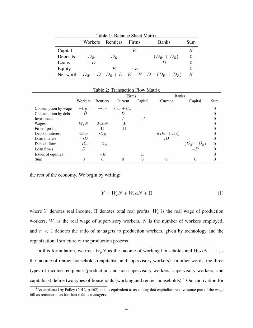
Table 1: Balance Sheet MatrixWorkers Rentiers Firms Banks Sum
Capital K K
Deposits D
W
D
R
�(DW
+D
R
) 0Loans �D D 0Equity E �E 0Net worth D
W
�D D
R
+ E K � E D � (DW
+D
R
) K
Table 2: Transaction Flow MatrixFirms Banks
Workers Rentiers Current Capital Current Capital Sum
Consumption by wage �CW
�CR
CW
+ CR
0
Consumption by debt � ˙D ˙D 0
Investment I �I 0
Wages Wp
N Wr
↵N �W 0
Firms’ profits ⇧ �⇧ 0
Deposit interest iDW
iDR
�i(DW
+DR
) 0
Loan interest �iD iD 0
Deposit flows � ˙DW
� ˙DR
(
˙DW
+
˙DR
) 0
Loan flows ˙D � ˙D 0
Issues of equities � ˙E ˙E 0
Sum 0 0 0 0 0 0 0
the rest of the economy. We begin by writing:
Y = W
p
N +W
r
↵N + ⇧ (1)
where Y denotes real income, ⇧ denotes total real profits, Wp
is the real wage of production
workers, Wr
is the real wage of supervisory workers, N is the number of workers employed,
and ↵ < 1 denotes the ratio of managers to production workers, given by technology and the
organizational structure of the production process.
In this formulation, we treat Wp
N as the income of working households and W
r
↵N + ⇧ as
the income of rentier households (capitalists and supervisory workers). In other words, the three
types of income recipients (production and non-supervisory workers, supervisory workers, and
capitalists) define two types of households (working and rentier households).5 Our motivation for5As explained by Palley (2012, p.462), this is equivalent to assuming that capitalists receive some part of the wage
bill as remuneration for their role as managers.
4
this bilateral distinction comes from the claim of Palley (2013b) that there is a marked distinction
(in terms of income and wealth shares) between the bottom 80 per cent and the top 20 per cent of
the US income distribution, with the bottom 80 per cent corresponding to the working class,6 and
the top 20 per cent corresponding to the middle class (including the upper middle class of capitalists
and the “working rich” who make up the top one per cent of the income distribution).7 As will
become clear in the next section, our ultimate purpose in making this bilateral distinction between
households is that we can impute to each identifiably different characteristics when it comes to
consumption behavior. First, we assume that working households conventionally consume a larger
fraction of their current income than do rentier households. Second, we assume that working
households borrow to finance some part of their current consumption, whereas rentier households
do not.
Bearing in mind the second of the two assumptions stated above, the balance sheet and trans-
action flow relationships between working and rentier households and the rest of the domestic
economy are described in the social accounting matrices (SAMs) in Tables 1 and 2. The SAMs in
Tables 1 and 2 serve to illustrate both how working and rentier households are related to each other,
and how the household sector and corporate sector of the economy fit together. There are several
noteworthy features of these SAMs. First, observe that because our purpose in this paper is to
model aggregate consumption spending, our behavioral analysis inevitably focuses on households.
The image of firms and banks that emerges from the SAMs in Tables 1 and 2 is highly stylized
and simplified. Firms do not borrow to finance investment expenditure, which is instead funded
solely by capitalists who purchase equities.8 Banks, meanwhile, are no more than passive interme-
diaries between households, earning no income from the intermediation services they provide and
accumulating no net worth.9
6Production and non-supervisory workers account for 80 per cent of all employees in the US economy.7The “working rich” refers to upper-level salaried employees who have, in increasing numbers, joined capitalist
households at the very top of the income distribution over the last thirty years. See Piketty and Saez (2003), Wolff andZacharias (2009) and Atkinson et al. (2011) on the evolution of “top incomes” in the US. See also Mohun (2006) onthe correct accounting treatment of the “wage” income earned by the “working rich”, and Wolff and Zacharias (2013)on the relationship between social class and the size distribution of income in the US.
8For simplicity, the price of equity is fixed and normalized to one.9Deposits are created endogenously in the model outlined below. Specifically, an increase in the demand for loans
5
Note also that the deposits of rentier households fund only part of the debt accumulated by
working households for the purpose of consumption expenditure. Part of the debt accumulated by
working households is funded by other working households, as a result of the fact that working
households are assumed to engage in some amount of saving out of their current income. In other
words, working households are assumed to save even as they accumulate debt to finance current
consumption.10 This behavior is consistent with stylized facts, and may be explained as follows.
First, working households are, themselves, heterogeneous: some engage in saving and do not debt-
finance current consumption, while others do not save and simultaneously consume more than they
earn by borrowing. Second, in an environment of fundamental uncertainty and imperfect credit
markets, it is reasonable for any individual household that wishes to consume in excess of current
income to simultaneously save and borrow. This is because uncertainty implies a precautionary
demand for liquidity to meet unforeseen contingencies, while imperfect credit markets mean that
dis-saving and borrowing are not perfect substitutes: a household is always legally entitled to draw
down its previously accumulated wealth, but has no similar entitlement to borrow.
3 Behavior
3.1 Production and Firms
Production in the economy is described by the following fixed coefficient production function:
Y = min{K, "Min[N,M/↵]} (2)
to finance additional expenditures results in endogenous income adjustment that insures the creation of balancingdeposits.
10As is clear from Tables 1 and 2, saving by working households results in the latter accumulating wealth exclusivelyin the form of interest-earning bank deposits: all corporate equity is owned by rentier households (Skott, 1989, 2014).As noted by Skott (2014), this is a simplified representation of observed differences in the portfolios of more- andless-affluent households. It is a departure, however, from the approach taken by Pasinetti (1962) and Palley (2012), inwhich physical capital is the only asset that households can own, as a result of which workers who save subsequentlyreceive some share of profit income. Clearly, the two approaches need not be mutually exclusive. We also assume,for simplicity, that firms do not use their cash flows to internally finance investment which, as previously noted, iswholly funded by that part of rentiers’ savings that is used to purchase corporate equity. Giving workers a portfoliochoice between deposits and corporate equity and allowing firms to internally finance some part of their investmentexpenditures are potentially interesting extensions of our model that we leave to future research.
6
where Y denotes real output and M denotes the number of managers.11 The fixed real wage earned
by workers is assumed to be a fraction of the real wage of managers, or:12
W
r
= �W
p
(3)
where � > 1. Total real wage income is then:
W = W
p
N +W
r
M (4)
) W = W
p
N + �W
p
↵N = (1 + �↵)Wp
N
If workers’ wage share of total income is denoted as !p
and managers’ wage share as !r
, we have
the following relationship:
!
r
= �↵!
p
(5)
Firms are characterized by their investment demand and mark-up pricing behavior. We treat
the pricing behavior of firms in standard neo-Kaleckian fashion: price is a mark up over unit labor
costs, reflecting an oligopolistic market structure (Harris, 1974; Asimakopulos, 1975). Such mark
up pricing behavior implies a standard expression for the gross profit share (⇡ = ⇧/Y ):
⇡ =⌧
1 + ⌧
(6)
where ⌧ is the (fixed) mark up applied to unit labor costs to determine prices.
Let r = ⇧/K denote the profit rate. Following Stockhammer (1999), our desired investment
rate (gK
= I/K) responds positively to the profit rate:
g
K
= 0 +
r
r (7)
The parameters in this investment function are positive: 0 captures the state of business confi-11A similar specification is adopted in Palley (2013a).12The same relationship holds in terms of the nominal wage since our model excludes inflation.
7
dence;13 and
r
captures the sensitivity of desired investment to the profit rate. The current profit
rate approximates the expected rate of return, and hence induces investment demand (Blecker,
2002; Stockhammer, 1999).
Note that the profit rate and hence the accumulation rate can be expressed in terms of the
capacity utilization rate (u = Y/K). The gross profit rate is just the product of the gross profit
share and the capacity utilization rate:
r = ⇡u (8)
Substitution into equation (7) then allows us to express the rate of accumulation in terms of the
capacity utilization rate:
g
K
= 0 +
r
⇡u (9)
3.2 Consumption
On the basis of the SAM in Table 2, aggregate consumption (C) can be written as:
C = C
W
+ C
R
+ D (10)
Note that borrowing by working households to finance consumption spending independently of
current income, D, results in the accumulation of a stock of debt by these households and the ac-
cumulation of an equivalent stock of financial assets by other households. The influence of debt
on consumption will become clear below when we explicitly model CW
and C
R
. The influence
of financial assets (and, indeed, wealth more generally) on consumption spending is, however,
overlooked in what follows for the sake of simplicity. Stylized facts (an extremely unequal distri-
bution of wealth – and particularly financial assets – coupled with small marginal propensities to
spend on the part of the richest members of society) suggest that the impact of wealth on aggregate13This term is often referred to as animal spirits.
8
consumption is modest.14
We next model borrowing by working households as:
D = �(CT � C
W
), � > 0 (11)
where C
T denotes a target level of consumption. The exact size of the adjustment parameter � is
sensitive to (inter alia) household borrowing norms and financial market lending norms. Unlike
Dutt (2005, 2006), we do not explicitly model a constraint on workers’ borrowing arising from
the preferences of lenders with respect to workers’ indebtedness. But as should be clear from the
definition of �, borrowing by workers is nevertheless constrained by rentier behavior. Hence rentier
concerns about the credit worthiness of working households, for example, will lower the value of
� and reduce workers’ borrowing, ceteris paribus. Note also that in equation (11), borrowing
only partially closes the gap between C
T and C
W
at any point in time. This means that working
households typically consume at a level that differs from the level of consumption to which they
aspire.15
Implicit in equations (10) and (11) is the notion that working households engage in a three-step
decision making process when determining their current consumption spending. First, they identify
a target level of consumption, CT . Second, they decide what part of current income to devote to
consumption spending, CW
. Finally, and in accordance with equation (11), they determine what
to borrow. Substituting (11) into (10), we arrive at:
C = (1� �)CW
+ �C
T + C
R
(12)
It follows from equation (12) that aggregate consumption is increasing in C
W
, CR
, and C
T .14For empirical evidence supporting these claims, see Wolff (2010) and Onaran et al. (2011).15Note that with CT > C
W
, ˙D � 0 in equation (11). In other words, the indebtedness of working householdsis strictly increasing over time. Although the model does not provide for deleveraging by working households as awhole unless CT < C
W
, it does not altogether ignore repayments of principal in the course of debt servicing. Hence˙D > 0 can be thought of as net new borrowing, with total borrowing exceeding repayments of principal for working
households as a whole whenever CT > CW
.
9
The consumption target CT captures the level of consumption to which working households
aspire in any given period and is specified as:
C
T = ⌘C
R
(13)
C
R
is the level of consumption of a contemporaneous reference group (in this model, rentier house-
holds). Workers observe the consumption patterns of rentier households and seek to emulate rentier
consumption. The larger is the emulation parameter ⌘, the higher the target level of consumption
and hence the more debt financed consumption is undertaken by workers, as shown in equation
(11). The consumption function we are modeling here can be thought of as sharing an affinity with
the relative income hypothesis associated with Duesenberry (1949).
Following Kim et al. (2014), we assume that households, in order to service the debts that ac-
crue as a result of their consumption behavior, pursue an ordered method of coping with increased
financial obligations. The motivation for this assumption comes from two sources. The first is the
argument that debt servicing expenditures by households are better thought of as a monetary outlay
undertaken volitionally by households, rather than an autonomous deduction from gross household
income (Cynamon and Fazzari, 2012). The second is the observations of Lusardi et al. (2011) who,
based on their analysis of data from the 2009 TNS Global Economic Crisis Survey of households
in 13 countries, suggest that “just as corporations tend to fund themselves first by drawing upon
internal funds, households address financial shocks first by drawing down savings” (Lusardi et al.,
2011, p.27).16
To allow for this “pecking order” theory of how households cope with increasing financial
demands, workers are assumed to consume a conventional fraction of their gross wage income,16Lusardi et al. (2011) study the ways in which households come up with emergency funds of 2000 dollars in 30
days in the event of a financial shock, finding that savings is the primary source of emergency funds for a large pro-portion of households. Their study does not provide direct evidence that households sacrifice savings to preserve theirconsumption expenditures following a financial shock. However, their results do suggest the possibility that, in theevent of a financial shock, households are willing to sacrifice savings while attempting to maintain their consumptionexpenditures. Further prima facie evidence in favor of this interpretation of household behavior can be found in Cy-namon and Fazzari (2015, Figure 3), which shows no trend in the ratio of consumption to income for the bottom 95%of the size distribution of income from 1989 to 2007, even as the debt to income ratio of this same group rose steadily(Cynamon and Fazzari, 2015, Figure 4).
10
and then use the residual to fund either debt servicing or current saving as the demands of the
former allow. In this scenario, then, working households regard saving as a luxury that is foregone
first (before consumption out of current income is affected) in the event that they confront higher
debt servicing obligations.17 In this case, the consumption functions of workers and rentiers are:
C
W
= c
W
W
p
N (14)
C
R
= c
⇡
[Wr
↵N + ⇧+ iD
R
] (15)
where, following a stylized fact, cW
> c
⇡
.18
It follows from the description of consumption behavior above that total saving by working
households is:
S
W
= (1� c
W
)Wp
N � iD
R
(16)
Note that it also follows from equations (15) and (16) that total saving in the economy can be
written as:
S = S
W
+ S
R
= [(1� c
W
) + (1� c
⇡
)�↵]Wp
N + (1� c
⇡
)⇧� c
⇡
iD
R
(17)
from which it is evident that @S/@DR
= �ic
⇡
< 0. In other words, aggregate saving – and hence,
for any given level of income, the average propensity to save of households – is decreasing in the
indebtedness of net debtor households. This result mirrors the coincidence of falling household
saving rates and rising household indebtedness actually observed in the US economy over the last
three decades (see, for example, Palley (2002); Barba and Pivetti (2009)).17The notion that working households treat saving as a luxury and otherwise live “hand to mouth,” using current
income in the first instance to fund current consumption and debt servicing obligations, dovetails with a second em-pirical observation made by Lusardi et al. (2011) – that approximately 25 percent of Americans self-report that theycertainly could not come up with 2,000 dollars in 30 days, while a further 19 percent claim that they could only do soby pawning or selling possessions or taking payday loans.
18Recall that c⇡
is associated with a rentier class made up of the top 20% of the size distribution of income. Asdemonstrated by Taylor et al. (2014) and Carvalho and Rezai (2015), this group has a markedly higher propensity tosave than other households.
11
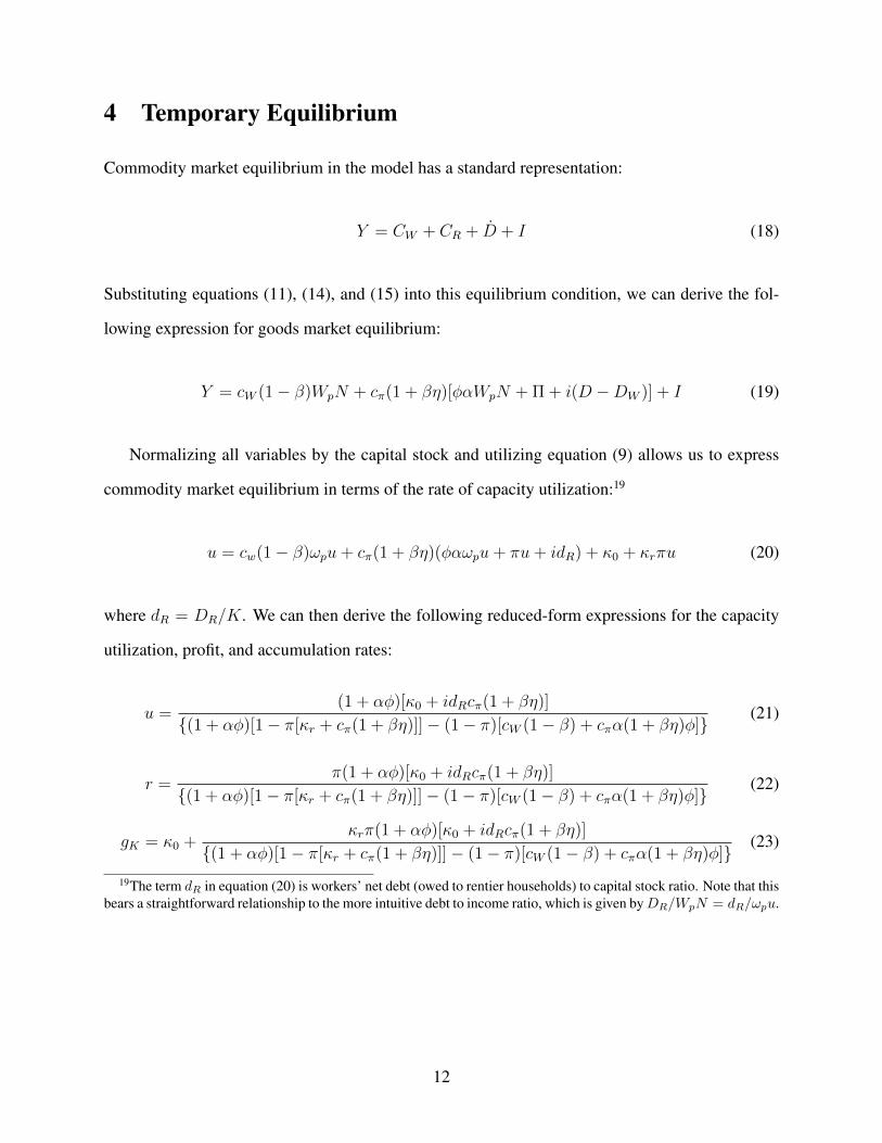
4 Temporary Equilibrium
Commodity market equilibrium in the model has a standard representation:
Y = C
W
+ C
R
+ D + I (18)
Substituting equations (11), (14), and (15) into this equilibrium condition, we can derive the fol-
lowing expression for goods market equilibrium:
Y = c
W
(1� �)Wp
N + c
⇡
(1 + �⌘)[�↵Wp
N + ⇧+ i(D �D
W
)] + I (19)
Normalizing all variables by the capital stock and utilizing equation (9) allows us to express
commodity market equilibrium in terms of the rate of capacity utilization:19
u = c
w
(1� �)!p
u+ c
⇡
(1 + �⌘)(�↵!p
u+ ⇡u+ id
R
) + 0 +
r
⇡u (20)
where d
R
= D
R
/K. We can then derive the following reduced-form expressions for the capacity
utilization, profit, and accumulation rates:
u =(1 + ↵�)[0 + id
R
c
⇡
(1 + �⌘)]
{(1 + ↵�)[1� ⇡[r
+ c
⇡
(1 + �⌘)]]� (1� ⇡)[cW
(1� �) + c
⇡
↵(1 + �⌘)�]} (21)
r =⇡(1 + ↵�)[0 + id
R
c
⇡
(1 + �⌘)]
{(1 + ↵�)[1� ⇡[r
+ c
⇡
(1 + �⌘)]]� (1� ⇡)[cW
(1� �) + c
⇡
↵(1 + �⌘)�]} (22)
g
K
= 0 +
r
⇡(1 + ↵�)[0 + id
R
c
⇡
(1 + �⌘)]
{(1 + ↵�)[1� ⇡[r
+ c
⇡
(1 + �⌘)]]� (1� ⇡)[cW
(1� �) + c
⇡
↵(1 + �⌘)�]} (23)
19The term dR
in equation (20) is workers’ net debt (owed to rentier households) to capital stock ratio. Note that thisbears a straightforward relationship to the more intuitive debt to income ratio, which is given by D
R
/Wp
N = dR
/!p
u.
12
Note that it follows from equations (1) and (5) that:
1� ⇡ = (1 + �↵)!p
(24)
) !
p
=1� ⇡
1 + �↵
On the basis of this result, !p
has been replaced with (1� ⇡)/(1 + ↵�) in the expressions for u, r,
and g
K
derived above.
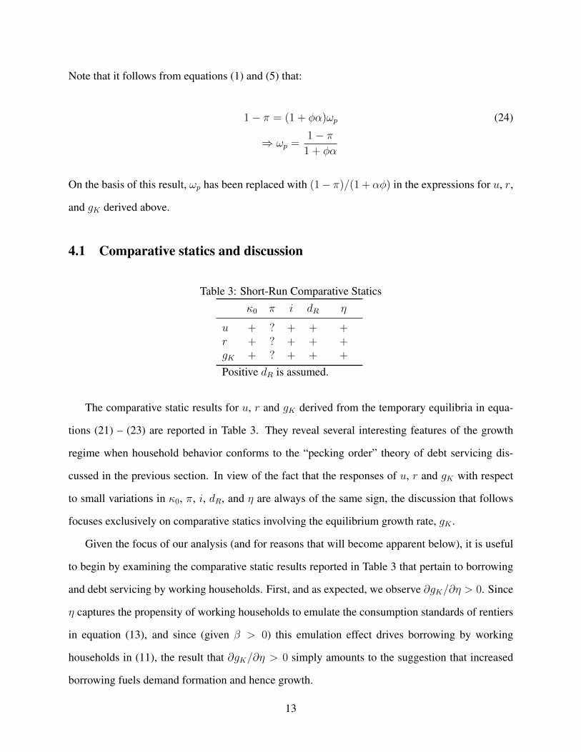
4.1 Comparative statics and discussion
Table 3: Short-Run Comparative Statics0 ⇡ i d
R
⌘
u + ? + + +r + ? + + +g
K
+ ? + + +
Positive d
R
is assumed.
The comparative static results for u, r and g
K
derived from the temporary equilibria in equa-
tions (21) – (23) are reported in Table 3. They reveal several interesting features of the growth
regime when household behavior conforms to the “pecking order” theory of debt servicing dis-
cussed in the previous section. In view of the fact that the responses of u, r and g
K
with respect
to small variations in 0, ⇡, i, dR
, and ⌘ are always of the same sign, the discussion that follows
focuses exclusively on comparative statics involving the equilibrium growth rate, gK
.
Given the focus of our analysis (and for reasons that will become apparent below), it is useful
to begin by examining the comparative static results reported in Table 3 that pertain to borrowing
and debt servicing by working households. First, and as expected, we observe @gK
/@⌘ > 0. Since
⌘ captures the propensity of working households to emulate the consumption standards of rentiers
in equation (13), and since (given � > 0) this emulation effect drives borrowing by working
households in (11), the result that @gK
/@⌘ > 0 simply amounts to the suggestion that increased
borrowing fuels demand formation and hence growth.
13
Of course, borrowing also results in debt accumulation and the servicing of debts sets up a flow
of transfer payments from debtors to creditors that (ceteris paribus) is conventionally thought to
create a deflationary drag in demand-led growth models.20 This is because of the higher marginal
propensity to consume of debtor households. It is therefore interesting to note that contrary to
this conventional wisdom, Table 3 draws attention to a seemingly perverse redistributive result:
@g
K
/@i, @g
K
/@d
R
> 0, indicating that increased debt servicing (which transfers income from
high marginal propensity to consume working households to low marginal propensity to consume
rentier households) boosts growth. Note that as a consequence of this, the economy is effectively
“super charged” by working household’s debt accumulation, because both borrowing (@gK
/@⌘ >
0) and the subsequent servicing of accumulated debt by working households contribute positively
to macroeconomic performance.
The intuition for this seemingly perverse redistributive result is straightforward.21 Because
of working households’ “pecking order” approach to debt servicing commitments, the transfer of
income towards rentiers associated with debt servicing involves a transfer of income not spent by
working households towards rentier households, who then apply a positive marginal propensity
to consume to additional income regardless of its source. In short, part of the income transferred
towards rentiers – all of which would otherwise constitute a leakage from the circular flow of
income – is transformed into an injection, because c⇡
> 0. This stimulates growth in a demand-led
economy, ceteris paribus. The comparative static results in the third and fourth columns of Table 3
thus illustrate the importance of the precise way that households are characterized as meeting their
debt servicing obligations, as originally emphasized by Kim et al. (2014).
The observations made above about the effects of borrowing and debt servicing on growth now
bring us to the comparative static results in the second column of Table 3, where the ambiguous
sign of @gK
/@⇡ reveals that the growth regime can be either wage- or profit-led. First note that
given the form of the investment function in equation (7):20See, for example, Dutt (2005, 2006) and Hein (2012, chpt.5).21See also Kim et al. (2014)
14
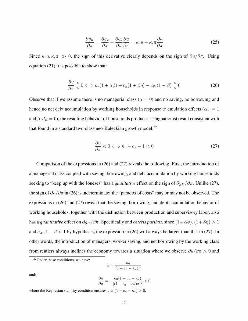
@g
K
@⇡
=@g
k
@⇡
+@g
k
@u
@u
@⇡
=
r
u+
r
⇡
@u
@⇡
(25)
Since
r
u,
r
⇡ � 0, the sign of this derivative clearly depends on the sign of @u/@⇡. Using
equation (21) it is possible to show that:
@u
@⇡
T 0 ()
r
(1 + ↵�) + c
⇡
(1 + �⌘)� c
W
(1� �) T 0 (26)
Observe that if we assume there is no managerial class (↵ = 0) and no saving, no borrowing and
hence no net debt accumulation by working households in response to emulation effects (cW
= 1
and �, d
R
= 0), the resulting behavior of households produces a stagnationist result consistent with
that found in a standard two-class neo-Kaleckian growth model:22
@u
@⇡
< 0 ()
r
+ c
⇡
� 1 < 0 (27)
Comparison of the expressions in (26) and (27) reveals the following. First, the introduction of
a managerial class coupled with saving, borrowing, and debt accumulation by working households
seeking to “keep up with the Joneses” has a qualitative effect on the sign of @gK
/@⇡. Unlike (27),
the sign of @u/@⇡ in (26) is indeterminate: the “paradox of costs” may or may not be observed. The
expressions in (26) and (27) reveal that the saving, borrowing, and debt accumulation behavior of
working households, together with the distinction between production and supervisory labor, also
has a quantitative effect on @g
K
/@⇡. Specifically and ceteris paribus, since (1+↵�), (1+�⌘) > 1
and c
W
, 1� � < 1 by hypothesis, the expression in (26) will always be larger than that in (27). In
other words, the introduction of managers, worker saving, and net borrowing by the working class
from rentiers always inclines the economy towards a situation where we observe @u/@⇡ > 0 and22Under these conditions, we have:
u =
0
(1� c⇡
� r
)⇡
and:@u
@⇡= � 0(1� c
⇡
� r
)
[(1� c⇡
� r
)⇡]2< 0
where the Keynesian stability condition ensures that (1� c⇡
� r
) > 0.
15
hence @g
K
/@⇡ > 0 (profit-led growth). The intuition for this last result is straightforward. First, it
arises because of the positive impact of emulation-induced borrowing and consumption on growth:
redistribution towards profit raises the consumption of the rentier class and reduces the capacity
of workers to consume from wage income, which together increase the difference between the
consumption target of and consumption out of wages by working households, and hence workers’
borrowing. These developments can increase the total consumption of working households even
as their consumption out of wage income necessarily falls.23 Second, the inclusion of a managerial
class that purchases equity generates a stronger profitability effect on investment expenditures,
as captured by the expression
r
(1 + ↵�) in equation (26).24 The expressions in (26) and (27)
clearly show that the conjunction of these effects is sufficient to ensure that the canonical effect
of a redistribution of income towards profits is modified so that the net effect on expenditures of a
rise in the profit share is more likely to be positive.
The critical question that remains is whether or not the growth regime is sustainable in the
long run. Sustainability requires that the long run steady state value of d
R
is compatible with
the feasibility condition for debt servicing by working households. Noting that the value of SW
in equation (16) must be greater than or equal to zero and normalizing the terms on the right
hand side of (16) by the capital stock, this feasibility condition can be stated as (1 � c
W
)!p
u �
id
R
. This condition is more restrictive than would be observed in the absence of the “pecking
order” approach to debt servicing commitments. Absent the “pecking order” approach, working
households would view their entire incomes as being, in the first instance, available for meeting
debt servicing commitments, instead of just some fraction (1 � c
W
) of this income. If the debt
servicing feasibility condition stated above is incompatible with the steady state value of dR
, the23It is for this reason that, in the event that the derivative in equation (25) proves to be positive, and in the spirit of
Kapeller and Schutz (2015), the resulting growth regime can be labeled consumption-driven, profit-led. As Kapellerand Schutz (2015) note, and as should also be clear from the results derived in this paper, the possibility of such aregime points towards the possible reconciliation of certain stylized facts of the Neoliberal era (redistribution towardsprofits accompanied by an increase in growth fueled by surging consumption spending and a fall in household savingrates) with the canonical neo-Kaleckian claim that the economy is wage-led – which claim would otherwise appear tobe at variance with the stylized facts just noted.
24The counterpart of this expression in equation (27) is r
< r
(1 + ↵�).
16
growth regime cannot be sustained in the long run and will eventually confront a crisis.25
5 Debt Dynamics
In this section, we investigate the debt dynamics associated with our model with a view to estab-
lishing whether or not growth is financially sustainable. To begin with, note that from the definition
of dR
, it follows that:
d
R
=�(CT � C
W
)� D
W
K
� g
K
d
R
(28)
= �(⌘CR
/K � C
W
/K)� D
W
/K � g
K
d
R
= �⌘c
⇡
(!r
u+ ⇡u+ id
R
)� (1 + �c
W
� c
W
)!p
u+ id
R
� g
K
d
R
It is clear from equation (28) that in order to completely express dR
in terms of the parameters of
our model, account needs to be taken of the expressions for u and g
K
in equations (21) and (23).
By setting d
R
= 0 we can then solve for and identify the stability properties of the steady state
value(s) of dR
. These operations are performed and reported in appendix A.
The analytical results reported in appendix A do not clearly reveal whether or not the two
steady state solutions for dR
(dR1 and d
R2) are positive (and therefore economically meaningful),
or which of these steady state solutions is stable. It does, however, seem likely that dR1 > d
R2,
based on observation of the signs of the final term on the RHS of these steady states solutions.26
Note, moreover, that, from Table 3, @gK
/@d
R
> 0. This implies that, in equation (28), the g
K
d
R
term is unambiguously increasing in d
R
. Inspection of equation (28) reveals that ceteris paribus, a
higher value of dR
will therefore generate a stronger stabilizing force, increasing the likelihood that
@d
R
/@d
R
< 0. It follows that the higher steady state value, dR1, should correspond to the stable
25Note that, in reality, a crisis can occur even before the aggregate feasibility condition stated above is violated, ifindividual borrowers begin to default with the result that lenders reduce the supply of loans to working households asa whole.
26As will become clear, our numerical solutions reveal that this intuition is correct.
17
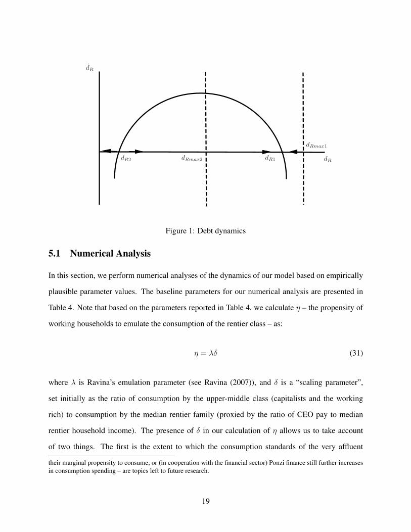
steady state solution of equation (28). Our numerical study in section 5.1 confirms this intuition.
Note that the inverse u-shape of the d
R
function implied by this result (and depicted in Figure 1)
differs from the conventional u-shaped relationship found in the literature (see, for example, Hein
(2012, pp.94-98)). This qualitative difference is further evidence of the importance that attaches to
the way that debtor households are conceived as managing their debt-servicing obligations.
We can also consider the proximity of the steady state values of dR
to the maximum feasible net
debt to capital ratio of working households, dRmax
, and in so doing consider the implications for
the sustainability of the growth regime. From the description of working households’ consumption
and debt servicing behavior provided earlier, it follows that the maximum debt servicing payment
that it is possible for workers to sustain is given by:
iD
Rmax
� (1� c
W
)Wp
N = 0 (29)
It therefore follows that:
d
Rmax
= (1� c
W
)!p
u/i (30)
=(c
W
� 1)0!p
i[�1 +
r
⇡ + c
W
!
p
(1� �) + c
⇡
(1 + �⌘)(⇡ + !
p
� c
W
!
p
+ !
p
↵�)]
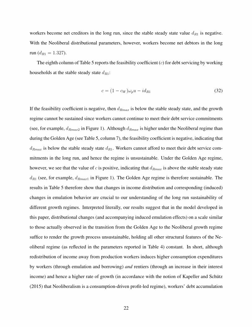
Now consider Figure 1, where d
R1 is the stable equilibrium.27 If dRmax
= d
Rmax1, then as long
as d
R
d
Rmax1 initially, the economy will converge to the stable, steady state debt to capital
ratio d
R1 and the accompanying steady-state growth rate will be sustainable indefinitely (ceteris
paribus). If, however, dRmax
= d
Rmax2, then even if dR
d
Rmax2 initially, unless it is also the
case that dR
< d
R2 (in which case the economy will move towards a situation in which working
households cease to be net debtors), the stability of dR1 will eventually pull the debt to capital ratio
above its maximum sustainable value. The consumption and borrowing behaviors of workers are
not sustainable in this case, and the economy will eventually experience a crisis.28
27In Figure 1, it is assumed for simplicity that both dR1 and d
R2 are positive. This need not be the case.28In the context of our model, a “crisis” refers only to a breakdown in the dynamics of the model as specified.
Exactly how the economy will react to these circumstances – whether, for example, working households will lower
18
dR1d
Rmax2
dRmax1
dR2
˙dR
dR
Figure 1: Debt dynamics
5.1 Numerical Analysis
In this section, we perform numerical analyses of the dynamics of our model based on empirically
plausible parameter values. The baseline parameters for our numerical analysis are presented in
Table 4. Note that based on the parameters reported in Table 4, we calculate ⌘ – the propensity of
working households to emulate the consumption of the rentier class – as:
⌘ = �� (31)
where � is Ravina’s emulation parameter (see Ravina (2007)), and � is a “scaling parameter”,
set initially as the ratio of consumption by the upper-middle class (capitalists and the working
rich) to consumption by the median rentier family (proxied by the ratio of CEO pay to median
rentier household income). The presence of � in our calculation of ⌘ allows us to take account
of two things. The first is the extent to which the consumption standards of the very affluent
their marginal propensity to consume, or (in cooperation with the financial sector) Ponzi finance still further increasesin consumption spending – are topics left to future research.
19
affect the aspirations of working households. This influence may be direct, arising as a result
of exposure to much-publicized “celebrity lifestyles”, or because of the propensity of working
households to believe in upward social mobility and the resulting need to consume in accordance
with their (expected future) social status (Wisman, 2009, 2013). Alternatively, it may be indirect,
resulting from the “expenditure cascades” discussed by Frank et al. (2014)).29 The second is the
growing income inequality within the rentier class in the top quintile of the income distribution.
The significance of these factors for our analysis will become apparent in what follows.
Keynesian and radical macroeconomists have distinguished the Golden Age growth regime
from the Neoliberal growth regime in the US, the stagflation of the 1970s marking the break be-
tween these regimes. One of the main differences between the two regimes is income distribution.
From 1943 to the late 1970s, all income classes experienced roughly the same income growth rate
of about 3 percent per annum. However, this began to change during the 1970s. For example, be-
tween 1973 and 2006, the average annual real income of the bottom 90 percent of households fell
while that of the top 1 percent increased 3.2-fold (Palma, 2009, p. 841). As these figures suggest,
between 1979 and 2003, income gains for US families have largely been concentrated at the very
top of the size distribution of income (Frank et al., 2014).
Table 5 demonstrates the implications for the debt dynamics of our model of variations in the
size of three key distributional parameters (!r
, !p
, and ⇡) between their Neoliberal values (as orig-
inally reported in Table 4) and their Golden Age values.30 Recall that ⌘ = ��, so the variations in ⌘
in the fourth column of Table 5 can be thought of as a product of a constant propensity to emulate
(�) and varying levels of income inequality within the top quintile of the income distribution (�)
as between the two growth regimes.31 With Golden Age distributional parameters, we see that29Bertrand and Morse (2013) provide empirical evidence of this phenomenon, which they term “trickle down con-
sumption”. The authors find that middle income US households would have saved 2.6–3.2 per cent more by themid-2000s had top incomes (defined as incomes in either the top quintile or top decile of the income distribution)grown at the same rate as median household income. Consistent with an emulation-based explanation of this outcome,they also find that it is middle income families’ expenditure on the most income elastic and visible goods and servicesthat is particularly responsive to top income growth.
30The latter appear in the first three columns of the second row of Table 5, and are calculated from the same sourcesreported in Table 4. Note also that the values of !
r
reported in Table 5 are calculated from the values of !p
, ↵ and �,given that !
r
= (1 + ↵�)!p
.31The value of � for the Golden Age is calculated from the same source reported in Table 4.
20
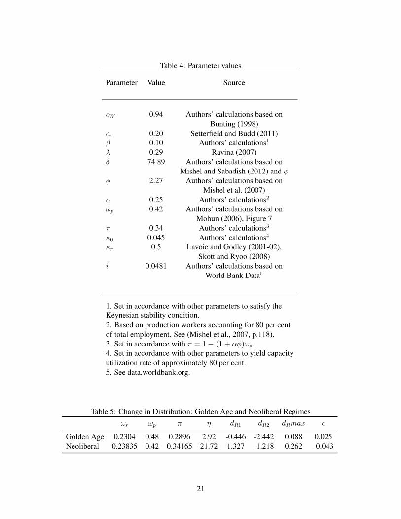
Table 4: Parameter values
Parameter Value Source
c
W
0.94 Authors’ calculations based onBunting (1998)
c
⇡
0.20 Setterfield and Budd (2011)� 0.10 Authors’ calculations1� 0.29 Ravina (2007)� 74.89 Authors’ calculations based on
Mishel and Sabadish (2012) and �
� 2.27 Authors’ calculations based onMishel et al. (2007)
↵ 0.25 Authors’ calculations2!
p
0.42 Authors’ calculations based onMohun (2006), Figure 7
⇡ 0.34 Authors’ calculations30 0.045 Authors’ calculations4
r
0.5 Lavoie and Godley (2001-02),Skott and Ryoo (2008)
i 0.0481 Authors’ calculations based onWorld Bank Data5
1. Set in accordance with other parameters to satisfy theKeynesian stability condition.2. Based on production workers accounting for 80 per centof total employment. See (Mishel et al., 2007, p.118).3. Set in accordance with ⇡ = 1� (1 + ↵�)!
p
.4. Set in accordance with other parameters to yield capacityutilization rate of approximately 80 per cent.5. See data.worldbank.org.
Table 5: Change in Distribution: Golden Age and Neoliberal Regimes!
r
!
p
⇡ ⌘ d
R1 d
R2 d
R
max c
Golden Age 0.2304 0.48 0.2896 2.92 -0.446 -2.442 0.088 0.025Neoliberal 0.23835 0.42 0.34165 21.72 1.327 -1.218 0.262 -0.043
21
workers become net creditors in the long run, since the stable steady state value d
R1 is negative.
With the Neoliberal distributional parameters, however, workers become net debtors in the long
run (dR1 = 1.327).
The eighth column of Table 5 reports the feasibility coefficient (c) for debt servicing by working
households at the stable steady state d
R1:
c = (1� c
W
)!p
u� id
R1 (32)
If the feasibility coefficient is negative, then d
Rmax
is below the stable steady state, and the growth
regime cannot be sustained since workers cannot continue to meet their debt service commitments
(see, for example, dRmax2 in Figure 1). Although d
Rmax
is higher under the Neoliberal regime than
during the Golden Age (see Table 5, column 7), the feasibility coefficient is negative, indicating that
d
Rmax
is below the stable steady state d
R1. Workers cannot afford to meet their debt service com-
mitments in the long run, and hence the regime is unsustainable. Under the Golden Age regime,
however, we see that the value of c is positive, indicating that dRmax
is above the stable steady state
d
R1 (see, for example, dRmax1 in Figure 1). The Golden Age regime is therefore sustainable. The
results in Table 5 therefore show that changes in income distribution and corresponding (induced)
changes in emulation behavior are crucial to our understanding of the long run sustainability of
different growth regimes. Interpreted literally, our results suggest that in the model developed in
this paper, distributional changes (and accompanying induced emulation effects) on a scale similar
to those actually observed in the transition from the Golden Age to the Neoliberal growth regime
suffice to render the growth process unsustainable, holding all other structural features of the Ne-
oliberal regime (as reflected in the parameters reported in Table 4) constant. In short, although
redistribution of income away from production workers induces higher consumption expenditures
by workers (through emulation and borrowing) and rentiers (through an increase in their interest
income) and hence a higher rate of growth (in accordance with the notion of Kapeller and Schutz
(2015) that Neoliberalism is a consumption-driven profit-led regime), workers’ debt accumulation
22
eventually becomes unsustainable. Workers’ consumption and borrowing behaviors must change if
the growth regime established by income redistribution away from production workers is to avoid
encountering a crisis.32
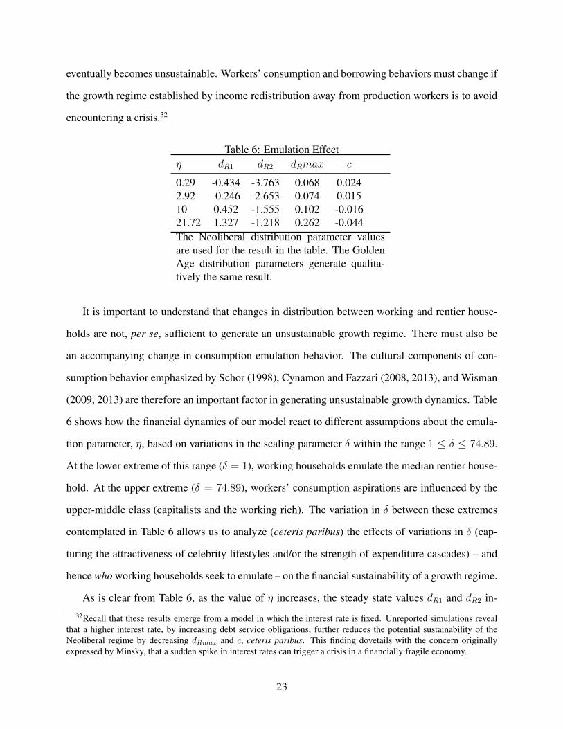
Table 6: Emulation Effect⌘ d
R1 d
R2 d
R
max c
0.29 -0.434 -3.763 0.068 0.0242.92 -0.246 -2.653 0.074 0.01510 0.452 -1.555 0.102 -0.01621.72 1.327 -1.218 0.262 -0.044The Neoliberal distribution parameter valuesare used for the result in the table. The GoldenAge distribution parameters generate qualita-tively the same result.
It is important to understand that changes in distribution between working and rentier house-
holds are not, per se, sufficient to generate an unsustainable growth regime. There must also be
an accompanying change in consumption emulation behavior. The cultural components of con-
sumption behavior emphasized by Schor (1998), Cynamon and Fazzari (2008, 2013), and Wisman
(2009, 2013) are therefore an important factor in generating unsustainable growth dynamics. Table
6 shows how the financial dynamics of our model react to different assumptions about the emula-
tion parameter, ⌘, based on variations in the scaling parameter � within the range 1 � 74.89.
At the lower extreme of this range (� = 1), working households emulate the median rentier house-
hold. At the upper extreme (� = 74.89), workers’ consumption aspirations are influenced by the
upper-middle class (capitalists and the working rich). The variation in � between these extremes
contemplated in Table 6 allows us to analyze (ceteris paribus) the effects of variations in � (cap-
turing the attractiveness of celebrity lifestyles and/or the strength of expenditure cascades) – and
hence who working households seek to emulate – on the financial sustainability of a growth regime.
As is clear from Table 6, as the value of ⌘ increases, the steady state values d
R1 and d
R2 in-32Recall that these results emerge from a model in which the interest rate is fixed. Unreported simulations reveal
that a higher interest rate, by increasing debt service obligations, further reduces the potential sustainability of theNeoliberal regime by decreasing d
Rmax
and c, ceteris paribus. This finding dovetails with the concern originallyexpressed by Minsky, that a sudden spike in interest rates can trigger a crisis in a financially fragile economy.
23
crease as well. As a higher ⌘ generates a higher capacity utilization rate, dRmax
also increases
in size. A higher emulation parameter also generates faster economic growth (as shown in Table
3). However, the calculated values of the feasibility coefficient c in Table 6 show that, with ever
higher values of ⌘ and ceteris paribus, the feasibility coefficient eventually becomes negative and
the resulting growth regime cannot be sustained in the long run. Recall that, given the propensity to
emulate, �, the size of ⌘ is related to the distributional parameter �.33 What this suggests is that in
addition to the redistribution of income between working and rentier households, the redistribution
of income within the top quintile of the income distribution towards the very affluent coupled with
the propensity of working households to emulate the consumption standards of the very affluent
(either directly or through expenditure cascades) is what drives the transition from a sustainable to
an unsustainable growth regime. This, in turn, suggests that in addition to the importance for the
properties of a growth regime that attaches to working households’ debt servicing behavior, impor-
tance also attaches to exactly who working households seek to emulate in the process of “keeping
up with the Joneses”, rather than simply whether or not such emulation effects exist. If either ex-
posure (through the media) to “celebrity lifestyles” or expenditure cascades are sufficiently strong,
the results in this paper suggest that the consequences for the sustainability of a growth regime
characterized by any given distribution of income between working and middle class households
are potentially adverse.
6 Conclusion
In this paper, we augment a conventional neo-Kaleckian model of growth and distribution with a
model of the household sector in which working households, motivated by a desire to emulate the
consumption standards of rentier households, borrow in order to finance some part of their total
consumption expenditures. The comparative static properties and debt-dynamics of the model are
then studied – the latter in an effort to identify whether or not growth is financially sustainable.33From equation (31), ⌘ = ��.
24
Our model yields three key results. First – and in tandem with the findings of Kim et al. (2014)
– it demonstrates the important effect on the characteristics of a growth regime of exactly how
working households manage their debt servicing obligations. Second, it illustrates the potential
significance of income redistribution away from working households for rendering an otherwise
stable (and seemingly well-performing) growth regime financially unsustainable. Finally, it reveals
that exactly who working households seek to emulate when formulating their consumption aspi-
rations has an important effect on whether or not a growth regime is financially sustainable. This
last result draws attention to the importance of growing inequality within the upper echelons of the
income distribution (as well as inequality between the upper echelons and the rest of the income
distribution) for the financial (un)sustainability of the growth process. It is hoped that these results
will contribute to our understanding of the origins of the Great Recession, and what is required to
restore robust (i.e., both sufficiently rapid and sustainable) economic growth.
7 Acknowledgment
Earlier versions of this paper were presented at the meetings of the Eastern Economic Associa-
tion, New York, May 2013, the FESSUD Annual Conference “Financialisation and the Financial
Crisis”, Amsterdam, October 2013, the 17th FMM Conference “The Jobs Crisis: Causes, Cures,
Constraints”, Berlin, October 2013, and the New School for Social Research, New York, February
2014. The authors would like to thank conference and seminar participants, Barry Cynamon, Steve
Fazzari, Eckhard Hein, Soon Ryoo, and two anonymous referees for their helpful comments. Any
remaining errors are our own. Mark Setterfield would like to thank the Institute for New Economic
Thinking for generous financial support that facilitated his work on this paper.
25
References
Asimakopulos, Athanasios (1975, August). “A Kaleckian theory of income distribution.” Cana-
dian Journal of Economics 8(3), 313–333.
Asimakopulos, Athanasios (1983, September-December). “Kalecki and Keynes on finance, invest-
ment and saving.” Cambridge Journal of Economics 7(3-4), 221–233.
Atkinson, Anthony B., Thomas Piketty, and Emmanuel Saez (2011). “Top incomes in the long run
of history.” Journal of Economic Literature 49, 3–71.
Barba, Aldo and Massimo Pivetti (2009). “Rising household debt: Its causes and macroeconomic
implications—a long-period analysis.” Cambridge Journal of Economics 33(1), 113–137.
Bertrand, Marianne and Adair Morse (2013). “Trickle down consumption.” NBER Working Paper
18883.
Blecker, Robert (2002). “Distribution, demand, and growth in neo-Kaleckian macro models.” In
Mark Setterfield, ed., The Economics of Demand-Led Growth: Challenging the Supply-Side
Vision of the Long Run, pp. 129–152. Cheltenham: Edward Elgar.
Bunting, David (1998). “Distributional basis of aggregate consumption.” Journal of Post Keynesian
Economics 20(3), 389–413.
Carvalho, Laura and Armon Rezai (2015). “Personal income inequality and aggregate demand.”
Cambridge Journal of Economics.
Cynamon, Barry Z. and Steven M. Fazzari (2008). “Household debt in the consumer age: Source
of growth—risk of collapse.” Capitalism and Society 3(2), Article 3.
Cynamon, Barry Z. and Steven M. Fazzari (2012). “Measuring household demand: a cash flow
measure.” Washington University in St Louis, mimeo.
26
Cynamon, Barry Z. and Steve M. Fazzari (2013). “The end of the consumer age.” In Steve M. Faz-
zari Cynamon, Barry Z. and Mark Setterfield, eds., After the Great Recession: The Struggle for
Economic Recovery and Growth, pp. 129–157. Cambridge University Press.
Cynamon, Barry Z. and Steven M. Fazzari (2015). “Inequality, the Great Recession and slow
recovery.” Cambridge Journal of Economics.
Duesenberry, J. S (1949). Income, Saving and the Theory of Consumer Behaviors. Cambridge,
MA: Harvard University Press.
Dutt, Amitava K. (2005). “Consumption, debt and growth.” In Mark Setterfield, ed., Interactions
in Analytical Political Economy, pp. 155–78. Armonk, NY: M.E. Sharpe.
Dutt, Amitava K. (2006). “Maturity, stagnation and consumer debt: a Steindlian approach.”
Metroeconomica 57, 339–364.
Dutt, Amitava K. (2008). “The dependence effect, consumption and happiness: Galbraith revis-
ited.” Review of Political Economy 20(4), 527–550.
Foster, John Bellamy and Fred Magdoff (2009). The Great Financial Crisis. New York, New York:
Monthly Review Press.
Frank, Robert H., Adam Seth Levine, and Oege Dijk (2014). “Expenditure cascades.” Review of
Behavioral Economics 1(12), 55–73.
Harris, Donald J. (1974). “The price policy of firms, the level of employment and distribution of
income in the short run.” Australian Economic Papers 13, 144–151.
Hein, Eckhard (2012). The Macroeconomics of Finance-dominated Capitalism - and its Crisis.
Cheltenham, UK: Edward Elgar.
Kapeller, Jakob and Bernhard Schutz (2015). “Conspicuous consumption, inequality and debt:
The nature of consumption-driven profit-led regimes.” Metroeconomica 66(1), 51–70.
27
Kim, Yun K (2012). “Emulation and consumer debt: Implications of keeping-up with the jones.”
Working Paper 1208, Trinity College.
Kim, Yun K, Mark Setterfield, and Yuan Mei (2014). “A theory of aggregate consumption.” Euro-
pean Journal of Economics and Economic Policies: Intervention 11(1), 31–49.
Kumhof, Michael and Romain Ranciere (2010). “Inequality, leverage and crises.” Working Paper
268, International Monetary Fund.
Lavoie, Marc and Wynne Godley (2001-02). “Kaleckian models of growth in a coherent stock-flow
monetary framework.” Journal of Post Keynesian Economics 24(2), 277–311.
Lusardi, A., D.J. Schneider, and P. Tufano (2011). “Financially fragile households: evidence and
implications.” Working paper, NBER Working Paper 17072.
Mishel, Lawrence, Jared Bernstein, and Sylvia Allegretto (2007). The State of Working America
2006/2007. Ithaca, NY: Cornell University Press.
Mishel, Lawrence and Natalie Sabadish (2012). “CEO pay and the top 1 percent: how executive
compensation and financial-sector pay have fueled income inequality.” Issue brief 331, Eco-
nomic Policy Institute.
Mohun, Simon (2006). “Distributive shares in the US economy, 1964-2001.” Cambridge Journal
of Economics 30(3), 347–370.
Onaran, Ozlem, Engelbert Stockhammer, and Lukas Grafl (2011). “Financialisation, income dis-
tribution and aggregate demand in the USA.” Cambridge Journal of Economics 35, 637–661.
Palley, Thomas I. (2002). “Economic contradictions coming home to roost? does the us economy
face a long-term aggregate demand generation problem?” Journal of Post Keynesian Eco-
nomics 25, 9–32.
Palley, Thomas I. (2009). “The relative permanent income theory of consumption: A synthetic
keynesduesenberryfriedman model.” Review of Political Economy 22(3), 4156.
28
Palley, Thomas I. (2012). “Wealth and wealth distribution in the neo-Kaleckian growth model.”
Journal of Post Keynesian Economics 34, 449–470.
Palley, Thomas I. (2013a). “A Kaldor-Hicks-Goodwin-Tobin-Kalecki model of growth and distri-
bution.” Metroeconomica 64(2), 319–345.
Palley, Thomas I. (2013b). “The middle class in macroeconomics and growth theory: a three
class neo-kaleckian-goodwin model.” Paper presented at the Meetings of the Eastern Economic
Association, New York, May 2013.
Palma, Jose Gabriel (2009). “The revenge of the market on the rentiers. why neo-liberal reports of
the end of history turned out to be premature.” Cambridge Journal of Economics 33, 829869.
Pasinetti, Luigi L. (1962). “Rate of profit and income distribution in relation to the rate of economic
growth.” Review of Economic Studies 29, 267–279.
Piketty, Thomas and Emmanuel Saez (2003, February). “Income inequality in the United States,
1913-1998.” Quarterly Journal of Economics 118(1), 1–41.
Ravina, Enrichetta (2007). “Habit formation and keeping up with the Joneses: evidence from
micro data.” http://ssrn.com/abstract=928248.
Robinson, Joan (1962). Essays in the theory of economic growth. New York, New York: St
Martin’s press.
Schor, Juliet B. (1998). The Overspent American: Upscaling, Downshifting, and the New Con-
sumer (1st ed.). New York, NY: Basic Books.
Setterfield, Mark (2013). “Wages, demand and us macroeconomic travails: Diagnosis and progno-
sis.” In Steve M. Fazzari Cynamon, Barry Z. and Mark Setterfield, eds., After the Great Reces-
sion: The Struggle for Economic Recovery and Growth, pp. 158–184. Cambridge: Cambridge
University Press.
29
Setterfield, Mark and Andrew Budd (2011). “A Keynes-Kalecki model of cyclical growth with
agent-based features.” In Philip Arestis, ed., Microeconomics, Macroeconomics and Economic
Policy: Essays in Honour of Malcolm Sawyer, pp. 228–50. London: Palgrave Macmillan.
Skott, Peter (1989). Conflict and effective demand in economic growth. Cambridge: Cambridge
University Press.
Skott, Peter (2014). “Increasing inequality and financial instability.” Review of Radical Political
Economics 45, 478–488.
Skott, Peter and Soon Ryoo (2008). “Macroeconomic implications of financialisation.” Cambridge
Journal of Economics 32(6), 827–862.
Stockhammer, Engelbert (1999). “Robinsonian and kaleckian growth. an update on Post-
Keynesian growth theories.” Working Paper 67, Vienna University of Economics and Business
Administration. http://ideas.repec.org/p/wiw/wiwwuw/wuwp067.html.
Taylor, Lance, Armon Rezai, Rishabh Kumar, N. H. Barbosa-Filho, and Laura Carvalho (2014).
“Wage increases, transfers, and the socially determined income distribution in the usa.” Techni-
cal report, Institute for New Economic Thinking Working Paper Series No. 11.
Wisman, Jon D. (2009). “Household saving, class identity, and conspicuous consumption.” Journal
of Economic Issues XLIII(1), 89–114.
Wisman, Jon D. (2013). “Wage stagnation, rising inequality and the financial crisis of 2008.”
Cambridge Journal of Economics 37, 921–945.
Wolff, E. N. (2010). “Recent trends in household wealth in the United States: rising debt and the
middle-class squeeze - an update to 2007.” Levy Economics Institute Working Paper No. 589.
Wolff, Edward N. and Ajit Zacharias (2009). “Household wealth and the measurement of economic
well-being in the united states.” Journal of Economic Inequality 7, 83–115.
30
Wolff, Edward N. and Ajit Zacharias (2013). “Class structure and economic inequality.” Cam-
bridge Journal of Economics 37, 1381–1406.
Zezza, Gennaro (2008). “U.s. growth, the housing market, and the distribution of income.” Journal
of Post Keynesian Economics 30(3), 375–401.
A Analysis of Debt Dynamics
From the definition of dR
, we see that:
d
R
=�(CT � C
W
)� D
W
K
� g
K
d
R
(33)
= �(⌘CR
/K � C
W
/K)� D
W
/K � g
K
d
R
= �⌘c
⇡
(!r
u+ ⇡u+ id
R
)� (1 + �c
W
� c
W
)!p
u+ id
R
� g
K
d
R
After substituting the solutions of u and g
K
into the above equation, we find that the debt
dynamics of our model yield the following steady states:
d
R1 =1
2c⇡
i
r
⇡(1 + �⌘){0[�1 + c
W
!
p
(1� �) + c
⇡
(1 + �⌘)(⇡ + !
p
↵�)] (34)
+i[1�
r
⇡ + c
W
!
p
(� � 1) + c
2⇡
�⌘(1 + �⌘)(!r
� !
p
↵�)� c
⇡
[⇡ � �⌘ + (1 +
r
)⇡�⌘
+!
p
(cW
(� � 1) + (1 + �⌘)(1 + ↵�))]]
+p
{4c⇡
i0r
⇡(1 + �⌘)[!p
(�1 + c
W
� c
W
�) + c⇡(⇡ + !
r
)�⌘]
+[�0 + 0[�c
W
!
p
(� � 1) + c
⇡
(1 + �⌘)(⇡ + !
p
↵�)] + i[1�
r
⇡ + c
W
!
p
(� � 1)
+c
2⇡
�⌘(1 + �⌘)(!r
� !
p
↵�)� c
⇡
[⇡ � �⌘ + (1 +
r
)⇡�⌘ + !
p
[cW
(� � 1) + (1 + �⌘)(1 + ↵�)]]]]2}}
31
d
R2 =1
2c⇡
i
r
⇡(1 + �⌘){0[�1 + c
W
!
p
(1� �) + c
⇡
(1 + �⌘)(⇡ + !
p
↵�)] (35)
+i[1�
r
⇡ + c
W
!
p
(� � 1) + c
2⇡
�⌘(1 + �⌘)(!r
� !
p
↵�)� c
⇡
[⇡ � �⌘ + (1 +
r
)⇡�⌘
+!
p
(cW
(� � 1) + (1 + �⌘)(1 + ↵�))]]
�p
{4c⇡
i0r
⇡(1 + �⌘)[!p
(�1 + c
W
� c
W
�) + c⇡(⇡ + !
r
)�⌘]
+[�0 + 0[�c
W
!
p
(� � 1) + c
⇡
(1 + �⌘)(⇡ + !
p
↵�)] + i[1�
r
⇡ + c
W
!
p
(� � 1)
+c
2⇡
�⌘(1 + �⌘)(!r
� !
p
↵�)� c
⇡
[⇡ � �⌘ + (1 +
r
)⇡�⌘ + !
p
[cW
(� � 1) + (1 + �⌘)(1 + ↵�)]]]]2}}
The stability of the equilibria is examined as follows:
@d
R
@d
R
|dR=dR1 =
1
�1 +
r
⇡ + c
W
!
p
(1� �) + c
⇡
(1 + �⌘)(⇡ + !
p
↵�)(36)
p{4c
⇡
i0r
⇡(1 + �⌘)[!p
(�1 + c
W
� c
W
�) + c⇡(⇡ + !
r
)�⌘]
+[�0 + 0[�c
W
!
p
(� � 1) + c
⇡
(1 + �⌘)(⇡ + !↵�)]
+i[1�
r
⇡ + c
W
!
p
(� � 1) + c
2⇡
�⌘(1 + �⌘)(!r
� !
p
↵�)
�c
⇡
(⇡ � �⌘ + (1 +
r
)⇡�⌘ + !
p
(cW
(� � 1) + (1 + �⌘)(1 + ↵�)))]]2}
@d
R
@d
R
|dR=dR2 =
�1
�1 +
r
⇡ + c
W
!
p
(1� �) + c
⇡
(1 + �⌘)(⇡ + !
p
↵�)(37)
p{4c
⇡
i0r
⇡(1 + �⌘)[!p
(�1 + c
W
� c
W
�) + c⇡(⇡ + !
r
)�⌘]
+[�0 + 0[�c
W
!
p
(� � 1) + c
⇡
(1 + �⌘)(⇡ + !↵�)]
+i[1�
r
⇡ + c
W
!
p
(� � 1) + c
2⇡
�⌘(1 + �⌘)(!r
� !
p
↵�)
�c
⇡
(⇡ � �⌘ + (1 +
r
)⇡�⌘ + !
p
(cW
(� � 1) + (1 + �⌘)(1 + ↵�)))]]2}
32
Recommended