Dataflow analysis
CS252r Spring 2011(Based on lecture notes by Jeff Foster)

© 2010 Stephen Chong, Harvard University
Control flow graph
•A control flow graph is a representation of a program that makes certain analyses (including dataflow analyses) easier
•A directed graph where•Each node represents a statement
•Edges represent control flow
•Statements may be•Assignments: x := y or x := y op z or x := op y
•Branches: goto L or if b then goto L•etc.
2

© 2010 Stephen Chong, Harvard University
Control-flow graph example
3
x := a + b;y := a * b;while (y > a) { a := a + 1; x := a + b}
x := a + b;
y := a * b;
y > a
a := a + 1;
x := a + b
© 2010 Stephen Chong, Harvard University
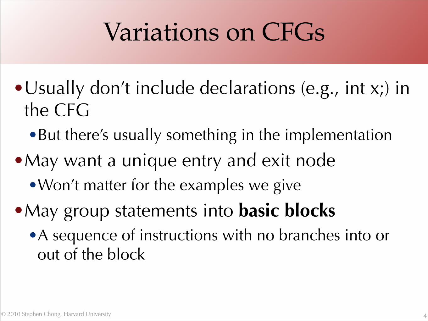
Variations on CFGs
•Usually don’t include declarations (e.g., int x;) in the CFG•But there’s usually something in the implementation
•May want a unique entry and exit node •Won’t matter for the examples we give
•May group statements into basic blocks•A sequence of instructions with no branches into or
out of the block
4
© 2010 Stephen Chong, Harvard University
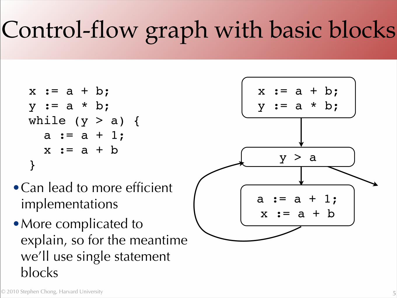
Control-flow graph with basic blocks
5
x := a + b;y := a * b;while (y > a) { a := a + 1; x := a + b}
x := a + b;y := a * b;
y > a
a := a + 1;x := a + b
•Can lead to more efficient implementations
•More complicated to explain, so for the meantime we’ll use single statement blocks

© 2010 Stephen Chong, Harvard University
Graph example with entry and exit
6
x := a + b;y := a * b;while (y > a) { a := a + 1; x := a + b}
x := a + b;
y := a * b;
y > a
a := a + 1;
x := a + b
exit
entry
•All nodes without a normal predecessor should be pointed to by entry
•All nodes with a successor should point to exit

© 2010 Stephen Chong, Harvard University
CFG vs AST
•CFGs are much simpler than ASTs
•Fewer forms, less redundancy, only simple expressions
•But AST is a more faithful representation •CFGs introduce temporaries
•Lose block structure of program
•ASTs are•Easier to report error + other messages
•Easier to explain to programmer•Easier to unparse to produce readable code
7
© 2010 Stephen Chong, Harvard University
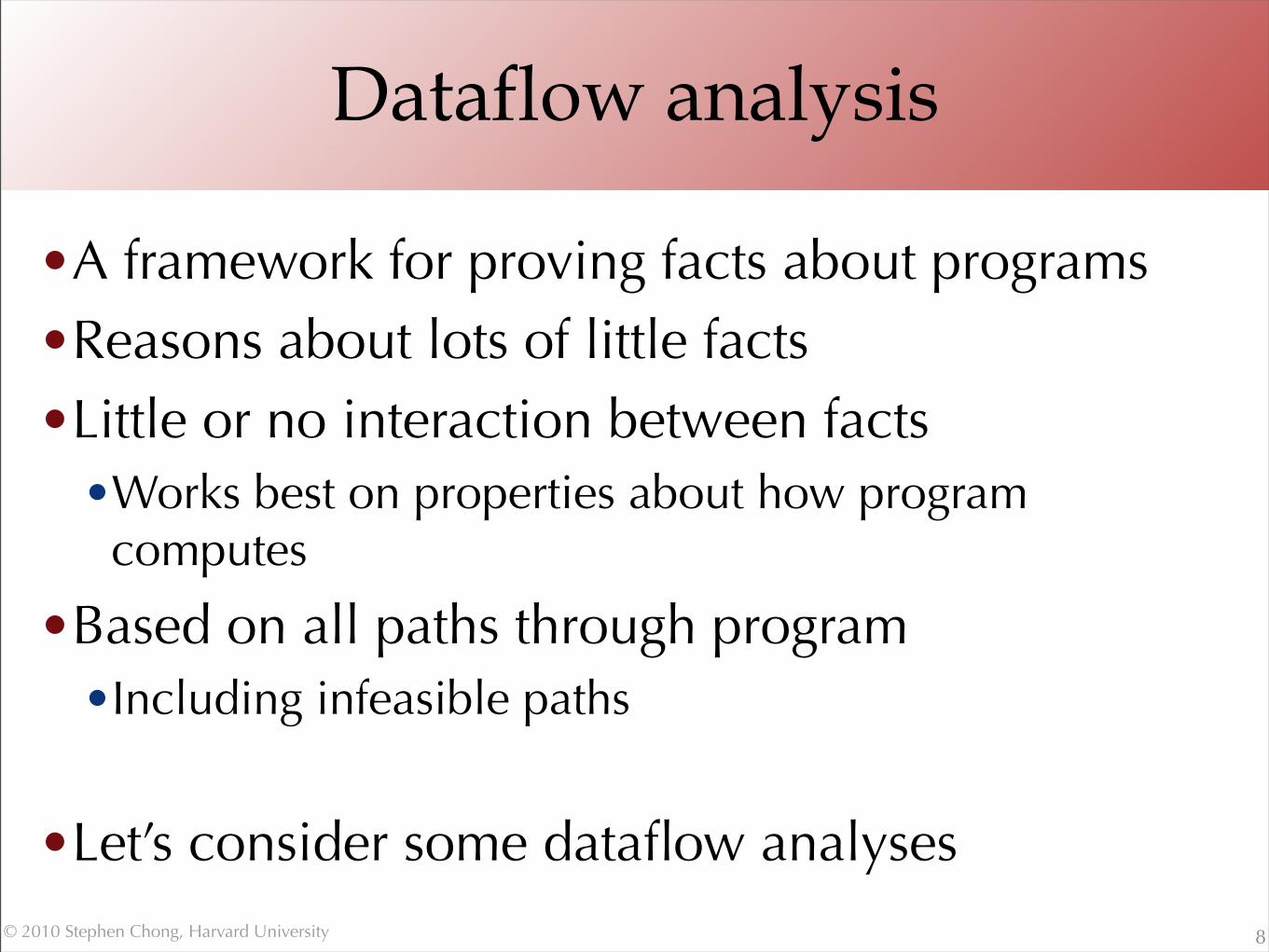
Dataflow analysis
•A framework for proving facts about programs•Reasons about lots of little facts•Little or no interaction between facts
•Works best on properties about how program computes
•Based on all paths through program•Including infeasible paths
•Let’s consider some dataflow analyses
8
© 2010 Stephen Chong, Harvard University
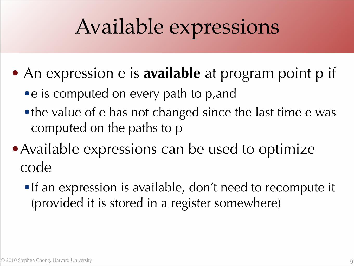
Available expressions
• An expression e is available at program point p if•e is computed on every path to p,and•the value of e has not changed since the last time e was
computed on the paths to p
•Available expressions can be used to optimize code•If an expression is available, don’t need to recompute it
(provided it is stored in a register somewhere)
9
© 2010 Stephen Chong, Harvard University
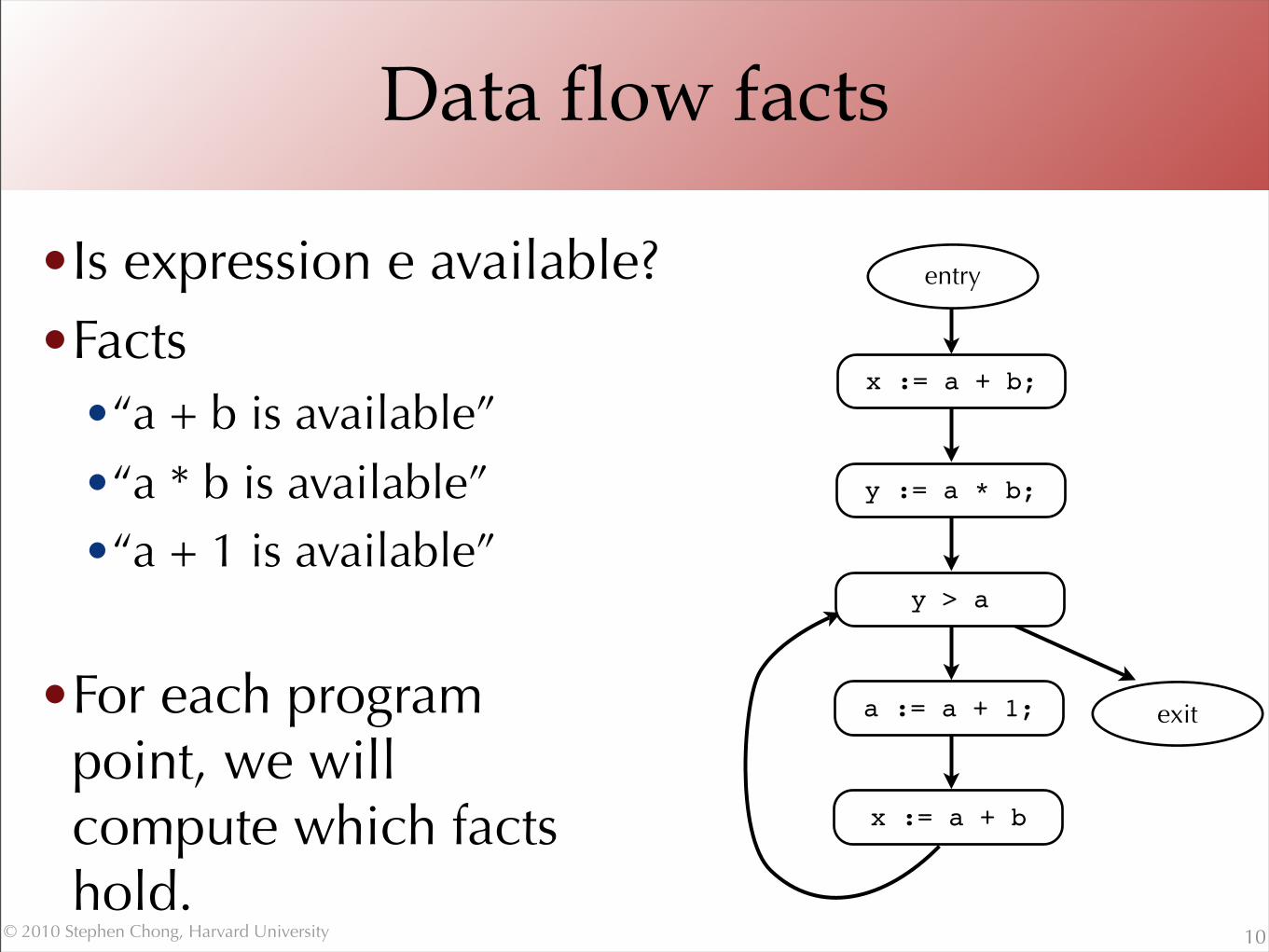
Data flow facts
•Is expression e available?•Facts
•“a + b is available”•“a * b is available”•“a + 1 is available”
•For each program point, we will compute which factshold.
10
x := a + b;
y := a * b;
y > a
a := a + 1;
x := a + b
exit
entry

© 2010 Stephen Chong, Harvard University
Gen and Kill
•What is the effect of each statement on the facts?
11
x := a + b;
y := a * b;
y > a
a := a + 1;
x := a + b
exit
entry
Stmt Gen Kill
x := a + b a + b
y := a * b a * b
y > a
a := a + 1a + 1a + ba * b
© 2010 Stephen Chong, Harvard University
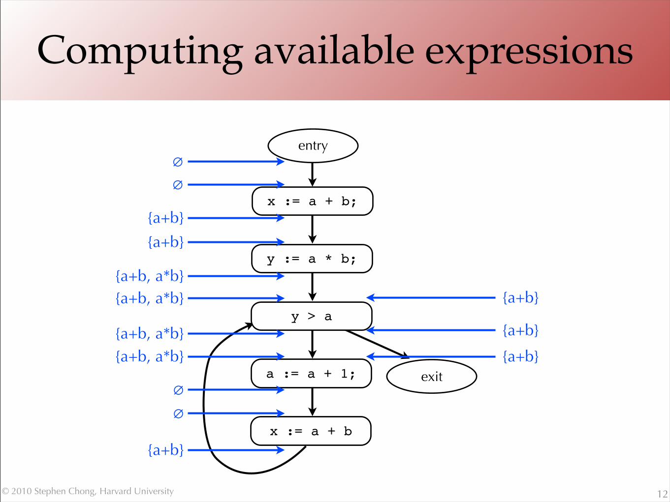
Computing available expressions
12
x := a + b;
y := a * b;
y > a
a := a + 1;
x := a + b
exit
entry∅
∅
{a+b}
{a+b}
{a+b, a*b}{a+b, a*b}
{a+b, a*b}{a+b, a*b}
∅
∅
{a+b}
{a+b}
{a+b}
{a+b}
© 2010 Stephen Chong, Harvard University
Terminology
•A join point is a program point where two or more branches meet
•Available expressions is a forward must analysis•Forward = Data flow from in to out•Must = At join points, only keep facts that hold on all
paths that are joined
13
© 2010 Stephen Chong, Harvard University
Data flow equations
•Let s be a statement•succs(s) = { immediate successor stmts of s }•preds(s) = { immediate predecessor stmts of s }•In(s) = program point just before executing s•Out(s) = program point just after executing s
•In(s) = ∩s’∈preds(s) Out(s’)
•Out(s) = Gen(s) ∪ (In(S) - Kill(s))
14
© 2010 Stephen Chong, Harvard University
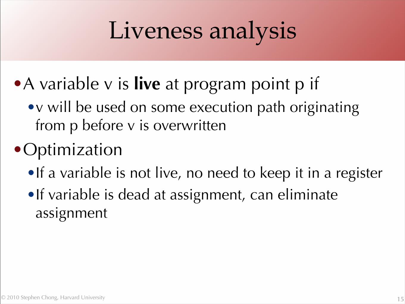
Liveness analysis
•A variable v is live at program point p if •v will be used on some execution path originating
from p before v is overwritten
•Optimization•If a variable is not live, no need to keep it in a register•If variable is dead at assignment, can eliminate
assignment
15

© 2010 Stephen Chong, Harvard University
Data flow equations
•Available expressions is a forward must analysis•Propagate facts in same direction as control flow
•Expression is available only if available on all paths
•Liveness is a backwards may analysis•To know if a variable is live, we need to look at the future
uses of it. We propagate facts backwards, from Out to In
•Variable is live if it is used on some path
•Out(s) = ∪s’∈succs(s) In(s’)
•In(s) = Gen(s) ∪ (Out(S) - Kill(s))
16
© 2010 Stephen Chong, Harvard University
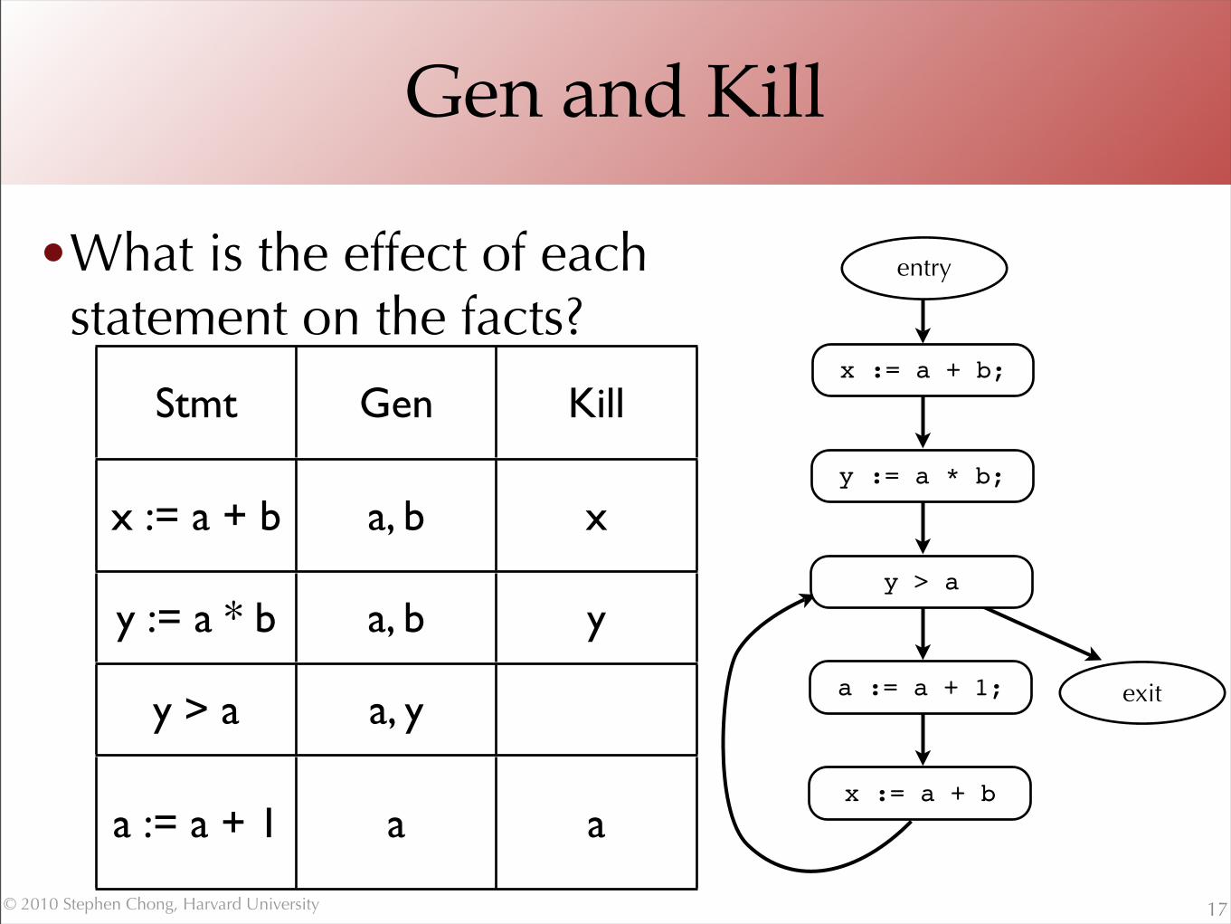
Gen and Kill
•What is the effect of each statement on the facts?
17
x := a + b;
y := a * b;
y > a
a := a + 1;
x := a + b
exit
entry
Stmt Gen Kill
x := a + b a, b x
y := a * b a, b y
y > a a, y
a := a + 1 a a

© 2010 Stephen Chong, Harvard University
Computing live variables
18
x := a + b;
y := a * b;
y > a
a := a + 1;
x := a + b
x
xx, y, a
x, y, a
x, a, b
x, a, b
a, b
x, y, a
y, a, b
y, a, b
y, a, b
x, y, a, b
x, y, a, b
x, y, a, b
x, y, a, b

© 2010 Stephen Chong, Harvard University
Very busy expressions
•An expression e is very busy at point p if •On every path from p, expression e is evaluated before
the value of e is changed
•Optimization•Can hoist very busy expression computation
•What kind of problem?•Forward or backward?•May or must?
19

© 2010 Stephen Chong, Harvard University
Reaching definitions
•A definition of a variable v is an assignment to v•A definition of variable v reaches point p if
•There is no intervening assignment to v•Also called def-use information
•What kind of problem?•Forward or backward?•May or must?
20
© 2010 Stephen Chong, Harvard University
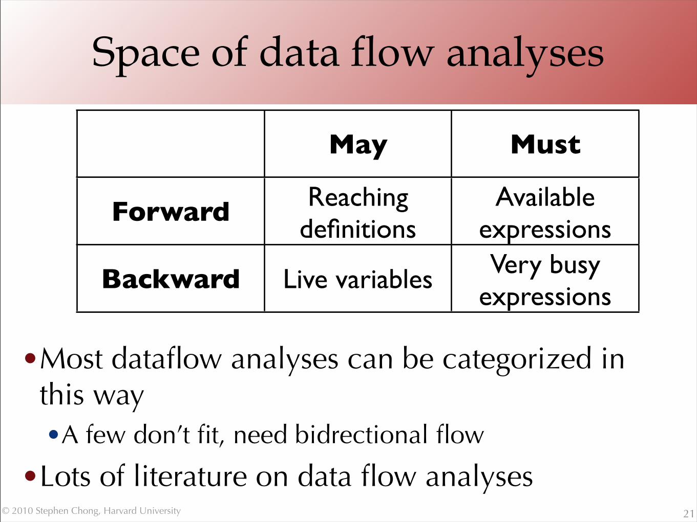
Space of data flow analyses
•Most dataflow analyses can be categorized in this way•A few don’t fit, need bidrectional flow
•Lots of literature on data flow analyses21
May Must
Forward Reaching definitions
Available expressions
Backward Live variables Very busy expressions
© 2010 Stephen Chong, Harvard University
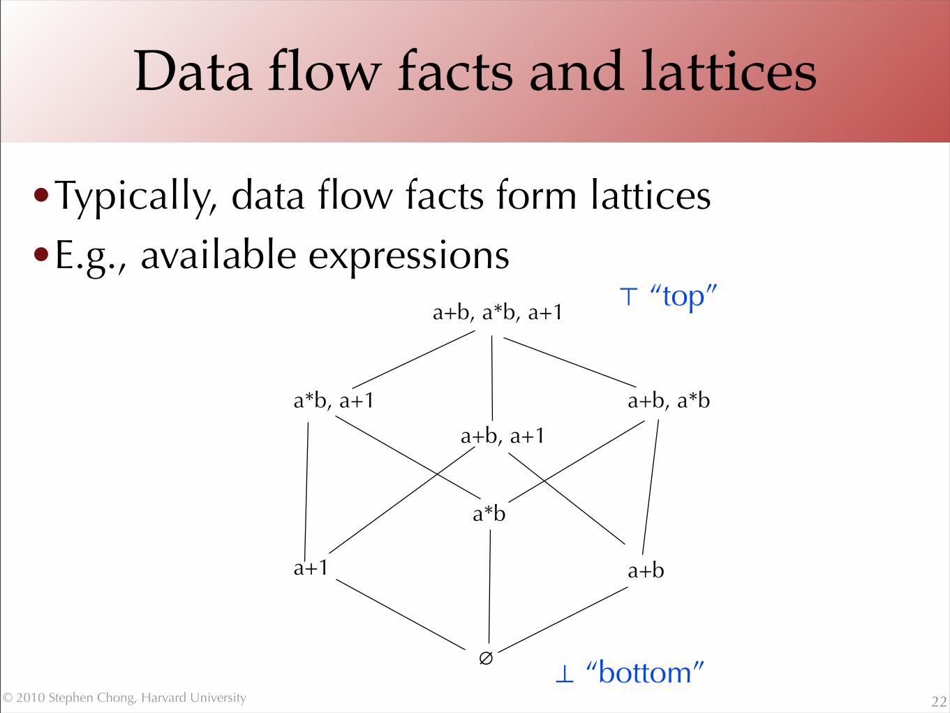
Data flow facts and lattices
•Typically, data flow facts form lattices•E.g., available expressions
22
a+b, a*b, a+1
a*b, a+1
a+b, a+1
a+b, a*b
a*b
a+1 a+b
∅
⊤ “top”
⊥ “bottom”

© 2010 Stephen Chong, Harvard University
Partial orders and lattices
•A partial order is a pair (P,≤) such that•≤ is a relation over P (≤ ⊆ P×P)
•≤ is reflexive, anti-symmetric, and transitive
•A partial order is a lattice if every two elements of P have a unique least upper bound and greatest lower bound.•⊓ is the meet operator: x ⊓ y is the greatest lower bound of x and y• x ⊓ y ≤ x and x ⊓ y ≤ y
• if z ≤ x and z ≤ y then z ≤ x ⊓ y
•⊔ is the join operator: x ⊔ y is the least upper bound of x and y• x ≤ x ⊔ y and y ≤ x ⊔ y
• if x ≤ z and y ≤ z then x ⊔ y ≤ z
• A join semi-lattice (meet semi-lattice) has only the join (meet) operator defined23

© 2010 Stephen Chong, Harvard University
Complete lattices
•A partially ordered set is a complete lattice if meet and join are defined for all subsets (i.e., not just for all pairs)
•A complete lattice always has a bottom element and a top element
•A finite lattice always has a bottom element and a top element
24

© 2010 Stephen Chong, Harvard University
Useful lattices
•(2S, ⊆) forms a lattice for any set S•2S is powerset of S, the set of all subsets of S.
•If (S, ≤) is a lattice, so is (S, ≥)•i.e., can “flip” the lattice
•Lattice for constant propagation
25
1 2 3 4 ...
⊤
⊥

© 2010 Stephen Chong, Harvard University
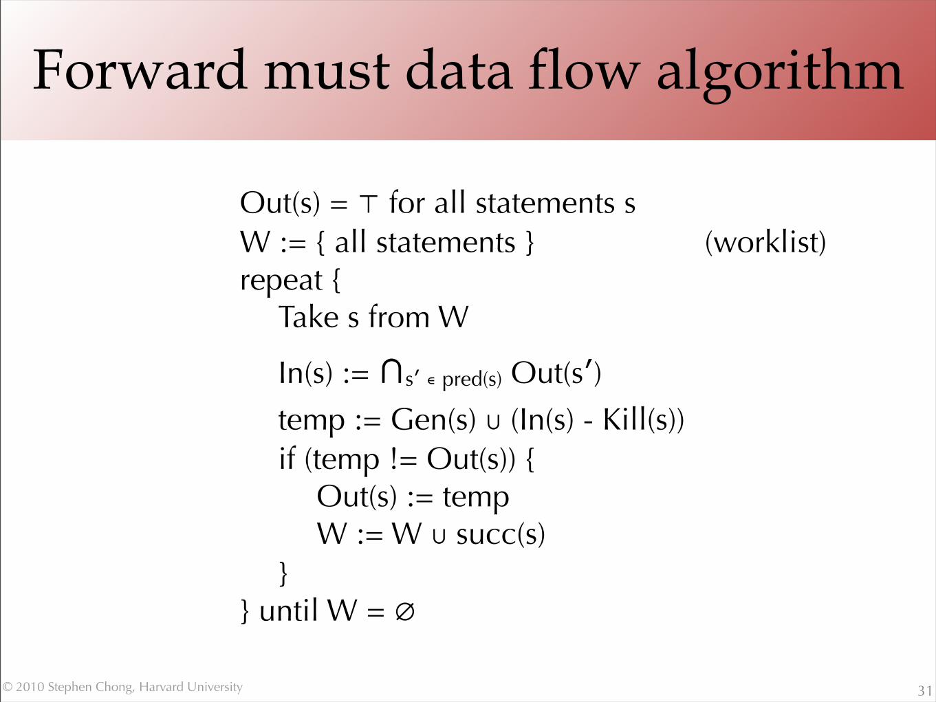
Forward must data flow algorithm
26
Out(s) = ⊤ for all statements sW := { all statements } (worklist) repeat {
Take s from W
In(s) := ∩s′ ∊ pred(s) Out(s′)temp := Gen(s) ∪ (In(s) - Kill(s))if (temp != Out(s)) {
Out(s) := temp W := W ∪ succ(s)
}} until W = ∅

© 2010 Stephen Chong, Harvard University
Monotonicity
•A function f on a partial order is monotonic if•if x ≤ y then f(x) ≤ f(y)
•Functions for computing In(s) and Out(s) are monotonic
•In(s) := ∩s′ ∊ pred(s) Out(s′)•temp := Gen(s) ∪ (In(s) - Kill(s))
• Putting them together: temp := fs(∩s′ ∊ pred(s) Out(s′))
27
A function fs of In(s)

© 2010 Stephen Chong, Harvard University
Termination
•We know the algorithm terminates
•In each iteration, either W gets smaller, or Out(s) decreases for some s•Since function is monotonic
•Lattice has only finite height, so for each s, Out(s) can decrease only finitely often
28
Out(s) = ⊤ for all statements sW := { all statements } repeat {
Take s from W
In(s) := ∩s′ ∊ pred(s) Out(s′)temp := Gen(s) ∪ (In(s) - Kill(s))if (temp != Out(s)) {
Out(s) := temp W := W ∪ succ(s)
}} until W = ∅
© 2010 Stephen Chong, Harvard University
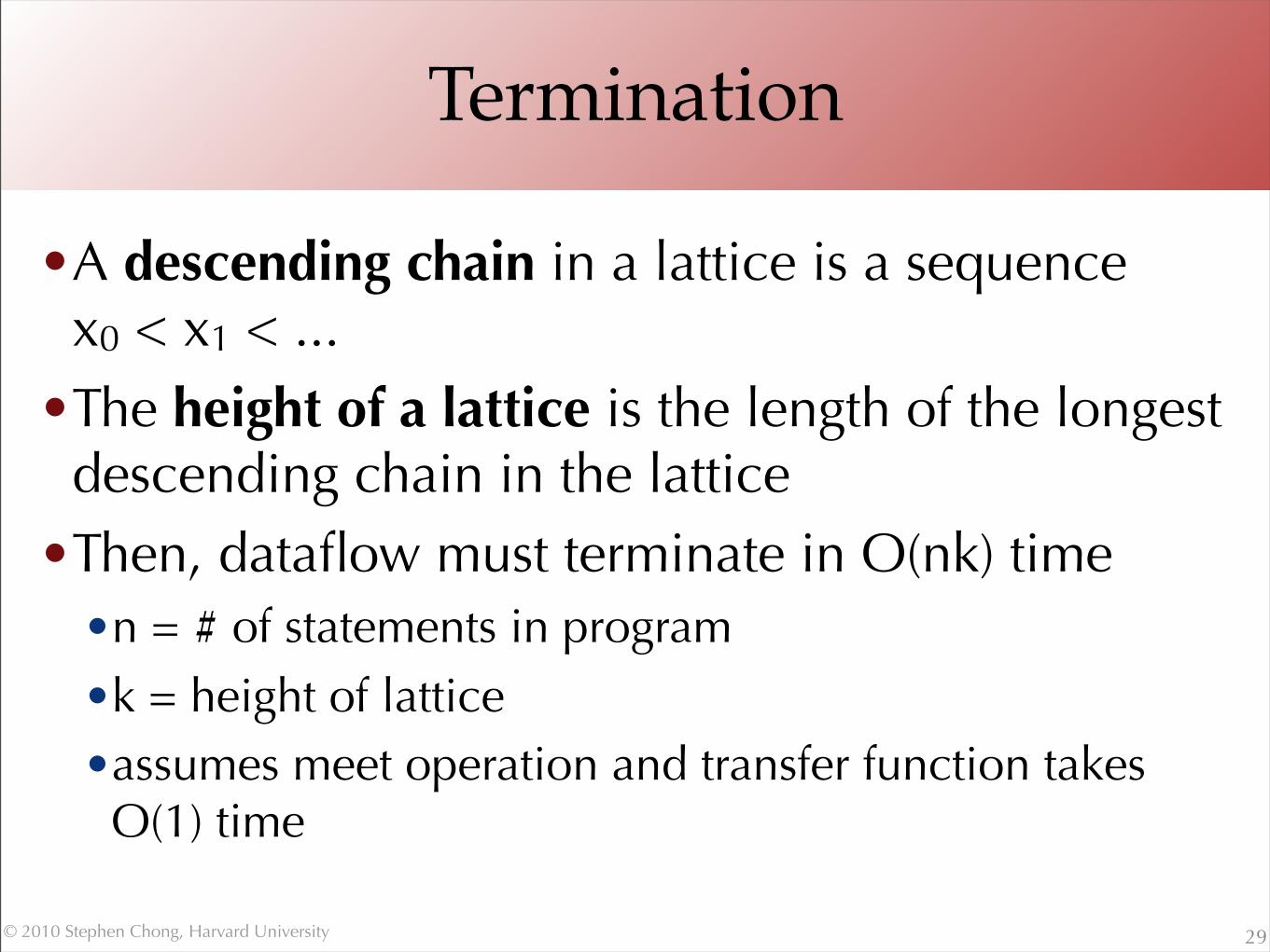
Termination
•A descending chain in a lattice is a sequencex0 < x1 < ...
•The height of a lattice is the length of the longest descending chain in the lattice
•Then, dataflow must terminate in O(nk) time •n = # of statements in program•k = height of lattice •assumes meet operation and transfer function takes
O(1) time
29

© 2010 Stephen Chong, Harvard University
Fixpoints
•Dataflow tradition: Start with Top, use meet•To do this, we need a meet semilattice with top• complete meet semilattice = meets defined for any set• finite height ensures termination
•Computes greatest fixpoint
•Denotational semantics tradition: Start with Bottom, use join•Computes least fixpoint
30
© 2010 Stephen Chong, Harvard University
Forward must data flow algorithm
31
Out(s) = ⊤ for all statements sW := { all statements } (worklist) repeat {
Take s from W
In(s) := ∩s′ ∊ pred(s) Out(s′)temp := Gen(s) ∪ (In(s) - Kill(s))if (temp != Out(s)) {
Out(s) := temp W := W ∪ succ(s)
}} until W = ∅
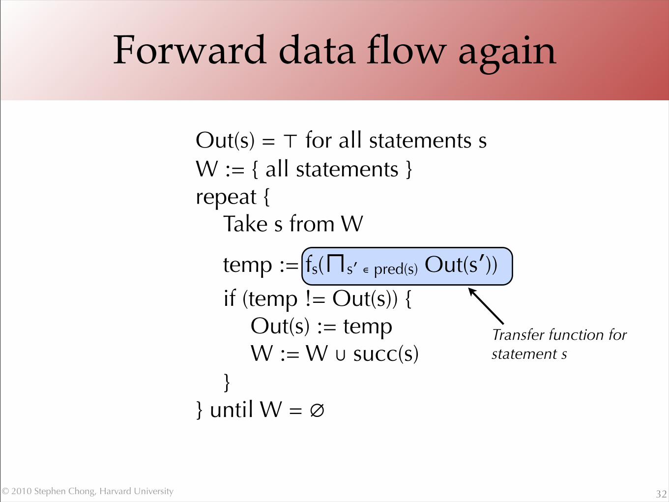
Transfer function forstatement s
© 2010 Stephen Chong, Harvard University
Forward data flow again
32
Out(s) = ⊤ for all statements sW := { all statements }repeat {
Take s from W
temp := fs(⊓s′ ∊ pred(s) Out(s′))if (temp != Out(s)) {
Out(s) := temp W := W ∪ succ(s)
}} until W = ∅
© 2010 Stephen Chong, Harvard University
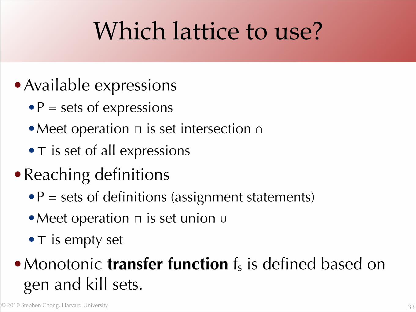
Which lattice to use?
•Available expressions•P = sets of expressions •Meet operation ⊓ is set intersection ∩
•⊤ is set of all expressions
•Reaching definitions•P = sets of definitions (assignment statements) •Meet operation ⊓ is set union ∪
•⊤ is empty set
•Monotonic transfer function fs is defined based on gen and kill sets.
33
© 2010 Stephen Chong, Harvard University
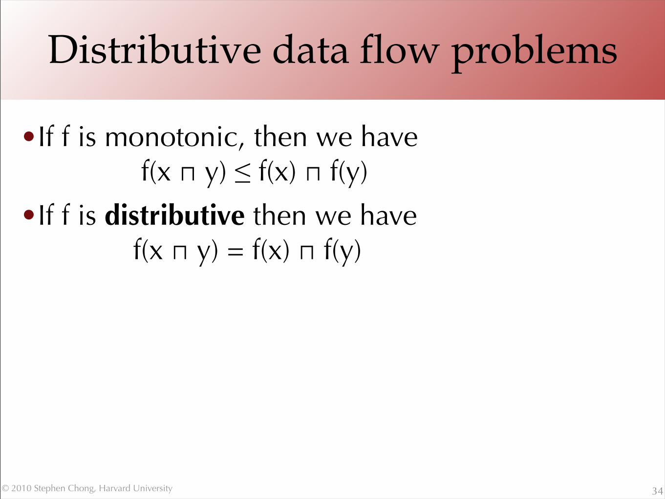
Distributive data flow problems
•If f is monotonic, then we have f(x ⊓ y) ≤ f(x) ⊓ f(y)
•If f is distributive then we have f(x ⊓ y) = f(x) ⊓ f(y)
34

© 2010 Stephen Chong, Harvard University
Benefit of distributivity
•Joins lose no information
• k(h(f(⊤) ⊓ g(⊤)))= k(h(f(⊤)) ⊓ h(g(⊤)))= k(h(f(⊤))) ⊓ k(h(g(⊤))))
35
f
h
k
g

© 2010 Stephen Chong, Harvard University
Accuracy of data flow analysis
•Ideally we would like to compute the meet over all paths (MOP) solution:•Let fs be the transfer function for statement s
•If p is a path s1,…,sn, let fp = fsn;...fs1•Let paths(s) be the set of paths from the entry to s
•MOP(s) = ⊓p∈paths(s) fp(⊤)
•If the transfer functions are distributive, then solving using the data flow equations in the standard way produces the MOP solution
36
© 2010 Stephen Chong, Harvard University
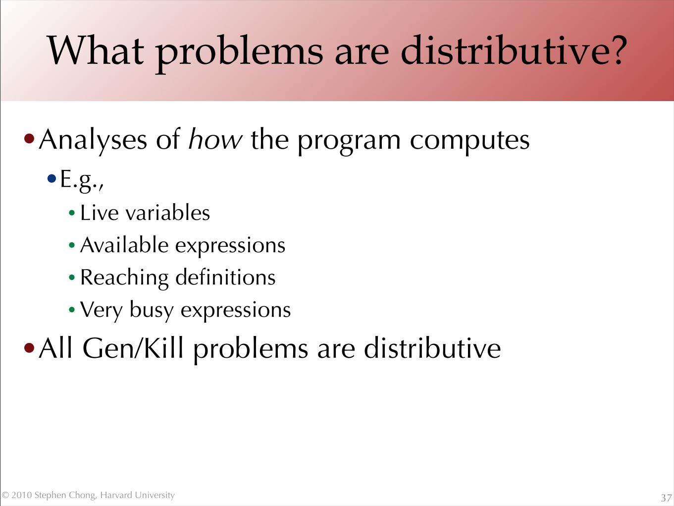
What problems are distributive?
•Analyses of how the program computes •E.g.,• Live variables •Available expressions•Reaching definitions•Very busy expressions
•All Gen/Kill problems are distributive
37

© 2010 Stephen Chong, Harvard University
Non-distributive example
•Constant propagation
•In general, analysis of what the program computes is not distributive
•Thm: MOP for In(s) will always be ⊑ iterative dataflow solution
38
y := 1;
z := x + y
y := 2;
x := 2; x := 1;
1 2 3 4 ...
⊤
⊥

© 2010 Stephen Chong, Harvard University
Practical implementation
•Data flow facts are assertions that are true or false at a program point
•Can represent set of facts as bit vector•Fact i represented by bit i•Intersection=bitwise and, union=bitwise or, etc
•“Only” a constant factor speedup•But very useful in practice
39

© 2010 Stephen Chong, Harvard University
Basic blocks
•A basic block is a sequence of statements such that•No branches to any statement except the first•No statement in the block branches except the last
•In practical data flow implementations•Compute Gen/Kill for each basic block•Compose transfer functions
•Store only In/Out for each basic block•Typical basic block is about 5 statements
40
© 2010 Stephen Chong, Harvard University
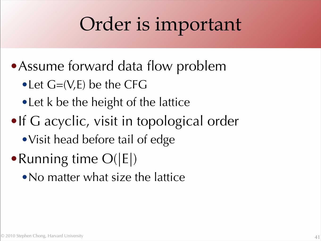
Order is important
•Assume forward data flow problem •Let G=(V,E) be the CFG •Let k be the height of the lattice
•If G acyclic, visit in topological order•Visit head before tail of edge
•Running time O(|E|)•No matter what size the lattice
41

© 2010 Stephen Chong, Harvard University
Order is important
• If G has cycles, visit in reverse postorder•Order from depth-first search
•Let Q = max # back edges on cycle-free path•Nesting depth•Back edge is from node to ancestor on DFS tree
•Then if ∀x. f(x) ≤ x (sufficient, but not necessary)
•Running time is O((Q + 1)|E|)
42

© 2010 Stephen Chong, Harvard University
Flow sensitivity
•Data flow analysis is flow sensitive•The order of statements is taken into account• I.e., we keep track of facts per program point
•Alternative: Flow-insensitive analysis•Analysis the same regardless of statement order•Standard example: types describe facts that are true at
all program points• /*x:int*/ x:=… /*x:int*/
43

© 2010 Stephen Chong, Harvard University
A problem...
•Consider following program
•Can pFile be NULL when used for fputs?•What dataflow analysis could we use to
determine if it is?44
FILE *pFile = NULL;if (debug) { pFile = fopen(“debuglog.txt”, “a”)}…if (debug) { fputs(“foo”, pFile);}

© 2010 Stephen Chong, Harvard University
Path sensitivity
45
pFile = ...
...
fputs(pFile)
...
debug
debug
pFile ≠ NULL∅
∅
∅

© 2010 Stephen Chong, Harvard University
Path sensitivity
• A path-sensitive analysis tracks data flow facts depending on the path taken• Path often represented by which branches of conditionals taken
• Can reason more accurately about correlated conditionals (or dependent conditionals) such as in previous example
• How can we make a path sensitive analysi• Could do a dataflow analysis where we track facts for each possible path
• But exponentially many paths make it difficult to scale
• Some research on scalable path sensitive analyses. We will discuss one next week
46
© 2010 Stephen Chong, Harvard University
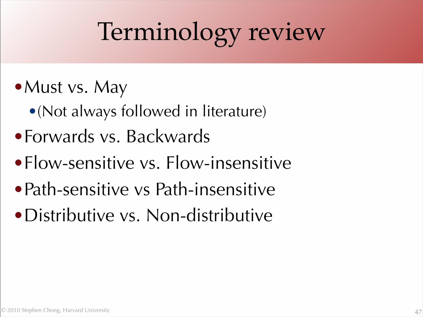
Terminology review
•Must vs. May•(Not always followed in literature)
•Forwards vs. Backwards•Flow-sensitive vs. Flow-insensitive•Path-sensitive vs Path-insensitive•Distributive vs. Non-distributive
47
© 2010 Stephen Chong, Harvard University
Dataflow analysis and the heap
•Data Flow is good at analyzing local variables•But what about values stored in the heap?•Not modeled in traditional data flow
•In practice: *x := e•Assume all data flow facts killed (!)•Or, assume write through x may affect any variable
whose address has been taken
•In general, hard to analyze pointers
48
Recommended