1
Data Mining: Concepts and Techniques
(3rd ed.)
— Chapter 8—
Jiawei Han, Micheline Kamber, and Jian Pei
University of Illinois at Urbana-Champaign &
Simon Fraser University
©2011 Han, Kamber & Pei. All rights reserved.
2
Chapter 8. Classification: Basic Concepts
� Classification: Basic Concepts
� Decision Tree Induction
� Bayes Classification Methods
� Rule-Based Classification
� Model Evaluation and Selection
� Techniques to Improve Classification Accuracy:
Ensemble Methods
� Summary

3
Supervised vs. Unsupervised Learning
� Supervised learning (classification)
� Supervision: The training data (observations,
measurements, etc.) are accompanied by labels indicating
the class of the observations
� New data is classified based on the training set
� Unsupervised learning (clustering)
� The class labels of training data is unknown
� Given a set of measurements, observations, etc. with the
aim of establishing the existence of classes or clusters in
the data

4
� Classification
� predicts categorical class labels (discrete or nominal)
� classifies data (constructs a model) based on the training set and the values (class labels) in a classifying attribute and uses it in classifying new data
� Numeric Prediction
� models continuous-valued functions, i.e., predicts unknown or missing values
� Typical applications
� Credit/loan approval:
� Medical diagnosis: if a tumor is cancerous or benign
� Fraud detection: if a transaction is fraudulent
� Web page categorization: which category it is
Prediction Problems: Classification vs. Numeric Prediction
5
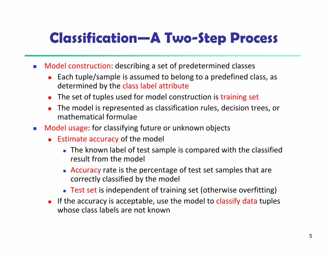
Classification—A Two-Step Process
� Model construction: describing a set of predetermined classes
� Each tuple/sample is assumed to belong to a predefined class, as determined by the class label attribute
� The set of tuples used for model construction is training set
� The model is represented as classification rules, decision trees, or mathematical formulae
� Model usage: for classifying future or unknown objects
� Estimate accuracy of the model
� The known label of test sample is compared with the classified result from the model
� Accuracy rate is the percentage of test set samples that are correctly classified by the model
� Test set is independent of training set (otherwise overfitting)
� If the accuracy is acceptable, use the model to classify data tuples whose class labels are not known
6
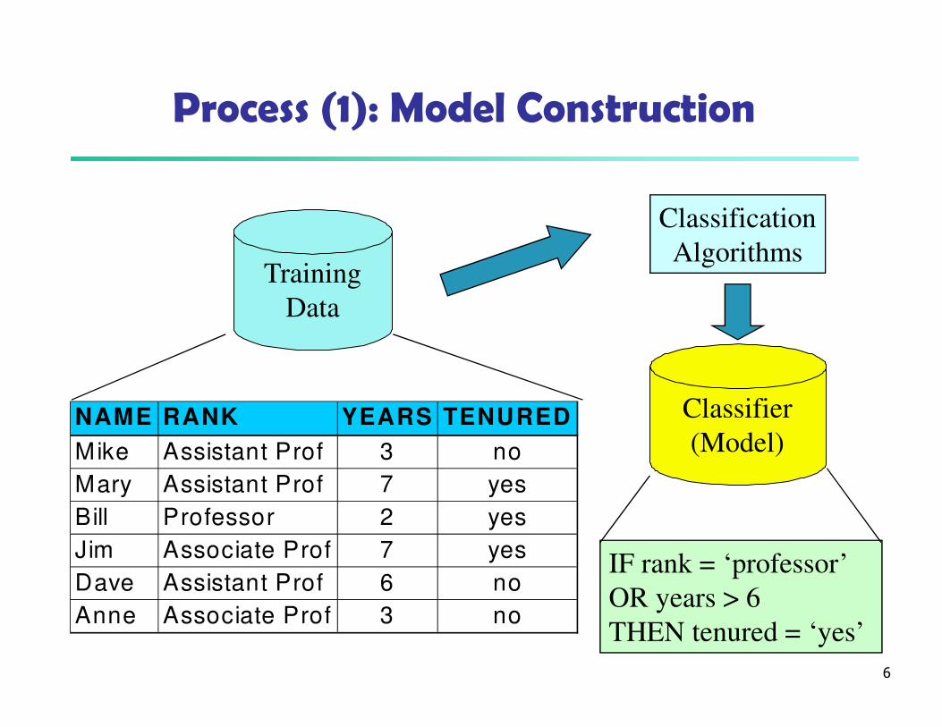
Process (1): Model Construction
Training
Data
NAME RANK YEARS TENURED
Mike Assistant Prof 3 no
Mary Assistant Prof 7 yes
Bill Professor 2 yes
Jim Associate Prof 7 yes
Dave Assistant Prof 6 no
Anne Associate Prof 3 no
Classification
Algorithms
IF rank = ‘professor’
OR years > 6
THEN tenured = ‘yes’
Classifier
(Model)

7
Process (2): Using the Model in Prediction
Classifier
Testing
Data
NAME RANK YEARS TENURED
Tom Assistant Prof 2 no
Merlisa Associate Prof 7 no
George Professor 5 yes
Joseph Assistant Prof 7 yes
Unseen Data
(Jeff, Professor, 4)
Tenured?

8
Chapter 8. Classification: Basic Concepts
� Classification: Basic Concepts
� Decision Tree Induction
� Bayes Classification Methods
� Rule-Based Classification
� Model Evaluation and Selection
� Techniques to Improve Classification Accuracy:
Ensemble Methods
� Summary
9
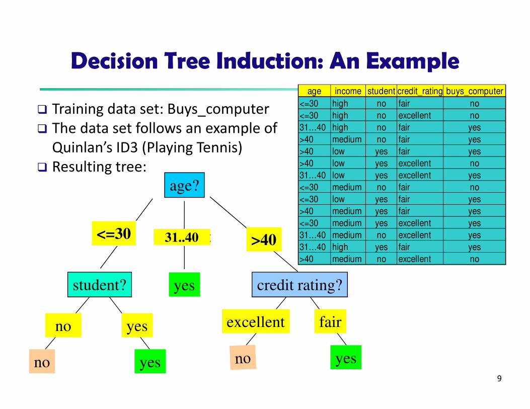
Decision Tree Induction: An Example
age?
overcast
student? credit rating?
<=30 >40
no yes yes
yes
31..40
fairexcellentyesno
age income student credit_rating buys_computer
<=30 high no fair no
<=30 high no excellent no
31…40 high no fair yes
>40 medium no fair yes
>40 low yes fair yes
>40 low yes excellent no
31…40 low yes excellent yes
<=30 medium no fair no
<=30 low yes fair yes
>40 medium yes fair yes
<=30 medium yes excellent yes
31…40 medium no excellent yes
31…40 high yes fair yes
>40 medium no excellent no
� Training data set: Buys_computer
� The data set follows an example of
Quinlan’s ID3 (Playing Tennis)
� Resulting tree:

10
Algorithm for Decision Tree Induction
� Basic algorithm (a greedy algorithm)
� Tree is constructed in a top-down recursive divide-and-
conquer manner
� At start, all the training examples are at the root
� Attributes are categorical (if continuous-valued, they are
discretized in advance)
� Examples are partitioned recursively based on selected
attributes
� Test attributes are selected on the basis of a heuristic or
statistical measure (e.g., information gain)
� Conditions for stopping partitioning
� All samples for a given node belong to the same class
� There are no remaining attributes for further partitioning –
majority voting is employed for classifying the leaf
� There are no samples left
11
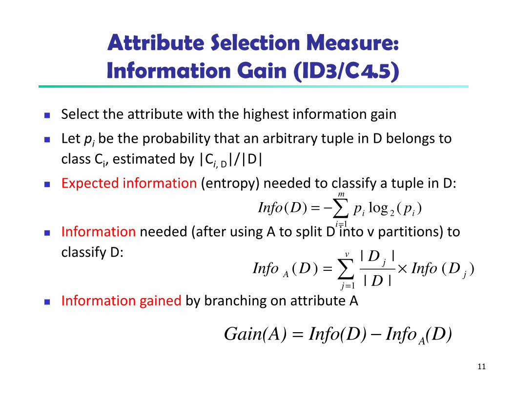
Attribute Selection Measure: Information Gain (ID3/C4.5)
� Select the attribute with the highest information gain
� Let pi be the probability that an arbitrary tuple in D belongs to
class Ci, estimated by |Ci, D|/|D|
� Expected information (entropy) needed to classify a tuple in D:
� Information needed (after using A to split D into v partitions) to
classify D:
� Information gained by branching on attribute A
)(log)( 2
1
i
m
i
i ppDInfo ∑=
−=
)(||
||)(
1
j
v
j
j
A DInfoD
DDInfo ×= ∑
=
(D)InfoInfo(D)Gain(A) A−=
12
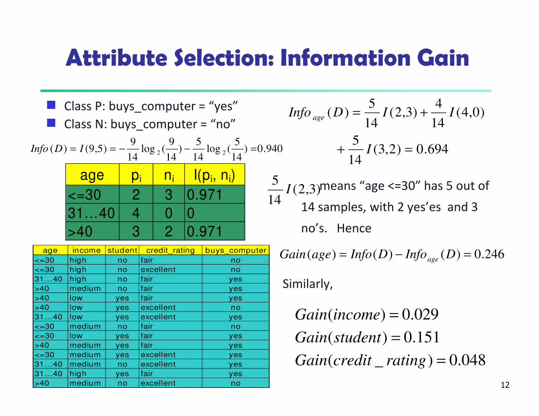
Attribute Selection: Information Gain
g Class P: buys_computer = “yes”
g Class N: buys_computer = “no”
means “age <=30” has 5 out of
14 samples, with 2 yes’es and 3
no’s. Hence
Similarly,
age pi ni I(pi, ni)
<=30 2 3 0.971
31…40 4 0 0
>40 3 2 0.971
694.0)2,3(14
5
)0,4(14
4)3,2(
14
5)(
=+
+=
I
IIDInfo age
048.0)_(
151.0)(
029.0)(
=
=
=
ratingcreditGain
studentGain
incomeGain
246.0)()()( =−= DInfoDInfoageGain age
age income student credit_rating buys_computer
<=30 high no fair no
<=30 high no excellent no
31…40 high no fair yes
>40 medium no fair yes
>40 low yes fair yes
>40 low yes excellent no
31…40 low yes excellent yes
<=30 medium no fair no
<=30 low yes fair yes
>40 medium yes fair yes
<=30 medium yes excellent yes
31…40 medium no excellent yes
31…40 high yes fair yes
>40 medium no excellent no
)3,2(14
5I
940.0)14
5(log
14
5)
14
9(log
14
9)5,9()( 22 =−−== IDInfo

13
Computing Information-Gain for Continuous-Valued Attributes
� Let attribute A be a continuous-valued attribute
� Must determine the best split point for A
� Sort the value A in increasing order
� Typically, the midpoint between each pair of adjacent values
is considered as a possible split point
� (ai+ai+1)/2 is the midpoint between the values of ai and ai+1
� The point with the minimum expected information
requirement for A is selected as the split-point for A
� Split:
� D1 is the set of tuples in D satisfying A ≤ split-point, and D2 is
the set of tuples in D satisfying A > split-point
14
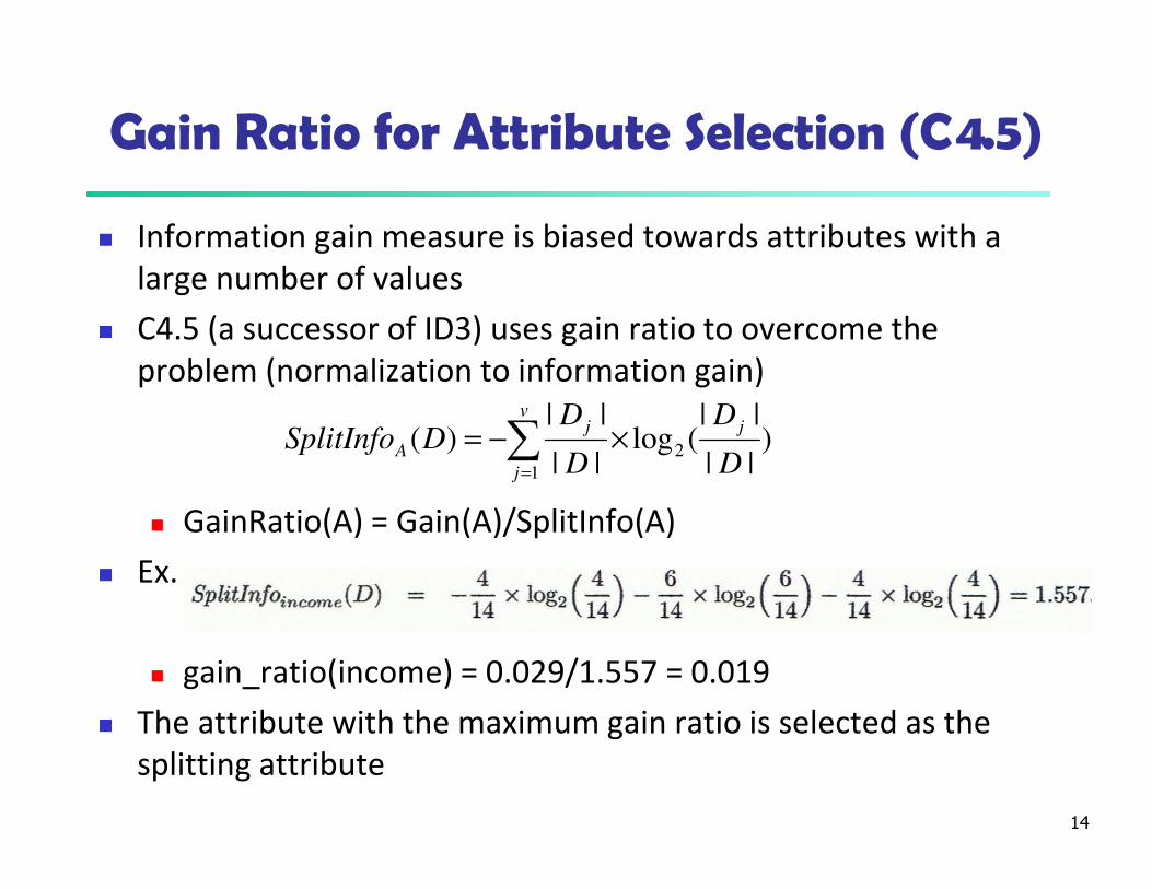
Gain Ratio for Attribute Selection (C4.5)
� Information gain measure is biased towards attributes with a
large number of values
� C4.5 (a successor of ID3) uses gain ratio to overcome the
problem (normalization to information gain)
� GainRatio(A) = Gain(A)/SplitInfo(A)
� Ex.
� gain_ratio(income) = 0.029/1.557 = 0.019
� The attribute with the maximum gain ratio is selected as the
splitting attribute
)||
||(log
||
||)( 2
1 D
D
D
DDSplitInfo
jv
j
j
A ×−= ∑=
15
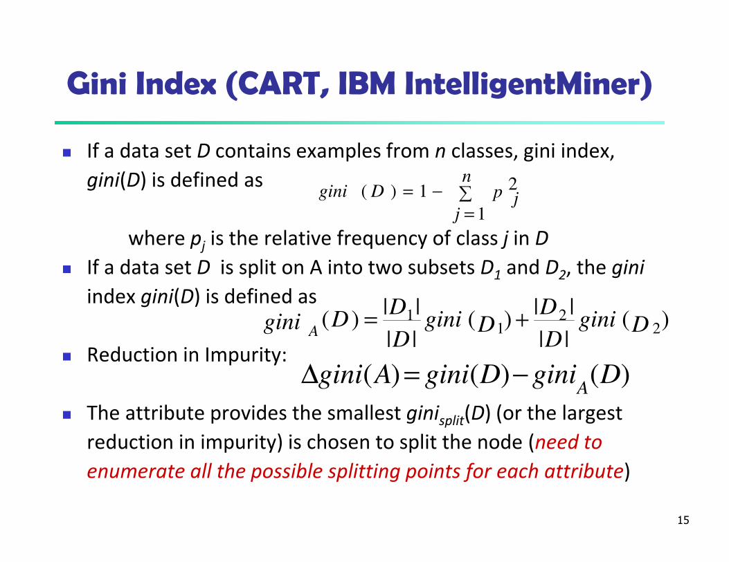
Gini Index (CART, IBM IntelligentMiner)
� If a data set D contains examples from n classes, gini index,
gini(D) is defined as
where pj is the relative frequency of class j in D
� If a data set D is split on A into two subsets D1 and D2, the gini
index gini(D) is defined as
� Reduction in Impurity:
� The attribute provides the smallest ginisplit(D) (or the largest
reduction in impurity) is chosen to split the node (need to
enumerate all the possible splitting points for each attribute)
∑=
−=n
j
p jDgini
1
21)(
)(||
||)(
||
||)( 2
21
1Dgini
D
DDgini
D
DDgini A
+=
)()()( DginiDginiAginiA
−=∆
16
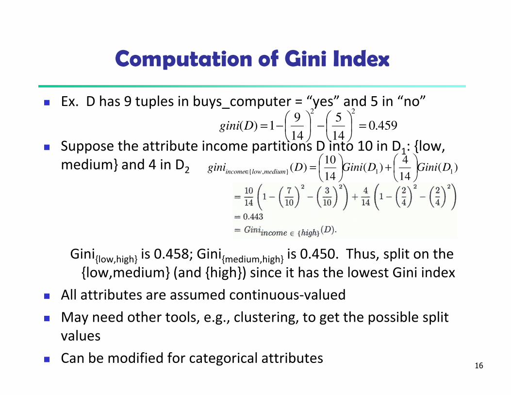
Computation of Gini Index
� Ex. D has 9 tuples in buys_computer = “yes” and 5 in “no”
� Suppose the attribute income partitions D into 10 in D1: {low,
medium} and 4 in D2
Gini{low,high} is 0.458; Gini{medium,high} is 0.450. Thus, split on the
{low,medium} (and {high}) since it has the lowest Gini index
� All attributes are assumed continuous-valued
� May need other tools, e.g., clustering, to get the possible split
values
� Can be modified for categorical attributes
459.014
5
14
91)(
22
=
−
−=Dgini
)(14
4)(
14
10)( 11},{ DGiniDGiniDgini mediumlowincome
+
=∈

17
Comparing Attribute Selection Measures
� The three measures, in general, return good results but
� Information gain:
� biased towards multivalued attributes
� Gain ratio:
� tends to prefer unbalanced splits in which one partition is
much smaller than the others
� Gini index:
� biased to multivalued attributes
� has difficulty when # of classes is large
� tends to favor tests that result in equal-sized partitions
and purity in both partitions
18
Other Attribute Selection Measures
� CHAID: a popular decision tree algorithm, measure based on χ2 test for
independence
� C-SEP: performs better than info. gain and gini index in certain cases
� G-statistic: has a close approximation to χ2 distribution
� MDL (Minimal Description Length) principle (i.e., the simplest solution is
preferred):
� The best tree as the one that requires the fewest # of bits to both (1)
encode the tree, and (2) encode the exceptions to the tree
� Multivariate splits (partition based on multiple variable combinations)
� CART: finds multivariate splits based on a linear comb. of attrs.
� Which attribute selection measure is the best?
� Most give good results, none is significantly superior than others

19
Overfitting and Tree Pruning
� Overfitting: An induced tree may overfit the training data
� Too many branches, some may reflect anomalies due to
noise or outliers
� Poor accuracy for unseen samples
� Two approaches to avoid overfitting
� Prepruning: Halt tree construction early ̵ do not split a node
if this would result in the goodness measure falling below a
threshold
� Difficult to choose an appropriate threshold
� Postpruning: Remove branches from a “fully grown” tree—
get a sequence of progressively pruned trees
� Use a set of data different from the training data to
decide which is the “best pruned tree”

20
Enhancements to Basic Decision Tree Induction
� Allow for continuous-valued attributes
� Dynamically define new discrete-valued attributes that
partition the continuous attribute value into a discrete set of
intervals
� Handle missing attribute values
� Assign the most common value of the attribute
� Assign probability to each of the possible values
� Attribute construction
� Create new attributes based on existing ones that are
sparsely represented
� This reduces fragmentation, repetition, and replication

21
Classification in Large Databases
� Classification—a classical problem extensively studied by
statisticians and machine learning researchers
� Scalability: Classifying data sets with millions of examples and
hundreds of attributes with reasonable speed
� Why is decision tree induction popular?
� relatively faster learning speed (than other classification methods)
� convertible to simple and easy to understand classification rules
� can use SQL queries for accessing databases
� comparable classification accuracy with other methods
� RainForest (VLDB’98 — Gehrke, Ramakrishnan & Ganti)
� Builds an AVC-list (attribute, value, class label)
22
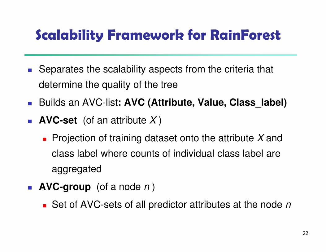
Scalability Framework for RainForest
� Separates the scalability aspects from the criteria that
determine the quality of the tree
� Builds an AVC-list: AVC (Attribute, Value, Class_label)
� AVC-set (of an attribute X )
� Projection of training dataset onto the attribute X and
class label where counts of individual class label are
aggregated
� AVC-group (of a node n )
� Set of AVC-sets of all predictor attributes at the node n
23
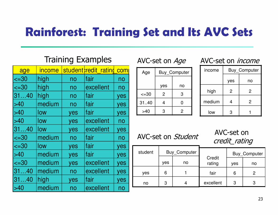
Rainforest: Training Set and Its AVC Sets
student Buy_Computer
yes no
yes 6 1
no 3 4
Age Buy_Computer
yes no
<=30 2 3
31..40 4 0
>40 3 2
Credit
rating
Buy_Computer
yes no
fair 6 2
excellent 3 3
age income studentcredit_ratingbuys_computer
<=30 high no fair no
<=30 high no excellent no
31…40 high no fair yes
>40 medium no fair yes
>40 low yes fair yes
>40 low yes excellent no
31…40 low yes excellent yes
<=30 medium no fair no
<=30 low yes fair yes
>40 medium yes fair yes
<=30 medium yes excellent yes
31…40 medium no excellent yes
31…40 high yes fair yes
>40 medium no excellent no
AVC-set on incomeAVC-set on Age
AVC-set on Student
Training Examplesincome Buy_Computer
yes no
high 2 2
medium 4 2
low 3 1
AVC-set on credit_rating

24
BOAT (Bootstrapped Optimistic Algorithm for Tree Construction)
� Use a statistical technique called bootstrapping to create
several smaller samples (subsets), each fits in memory
� Each subset is used to create a tree, resulting in several
trees
� These trees are examined and used to construct a new
tree T’
� It turns out that T’ is very close to the tree that would
be generated using the whole data set together
� Adv: requires only two scans of DB, an incremental alg.

November 1, 2015 Data Mining: Concepts and Techniques 25
Presentation of Classification Results

November 1, 2015 Data Mining: Concepts and Techniques 26
Visualization of a Decision Tree in SGI/MineSet 3.0
Data Mining: Concepts and Techniques 27
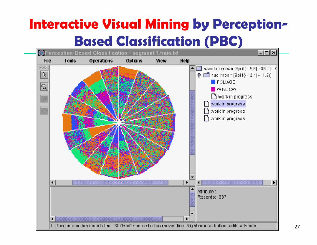
Interactive Visual Mining by Perception-Based Classification (PBC)

28
Chapter 8. Classification: Basic Concepts
� Classification: Basic Concepts
� Decision Tree Induction
� Bayes Classification Methods
� Rule-Based Classification
� Model Evaluation and Selection
� Techniques to Improve Classification Accuracy:
Ensemble Methods
� Summary
29
Bayesian Classification: Why?
� A statistical classifier: performs probabilistic prediction, i.e.,
predicts class membership probabilities
� Foundation: Based on Bayes’ Theorem.
� Performance: A simple Bayesian classifier, naïve Bayesian
classifier, has comparable performance with decision tree and
selected neural network classifiers
� Incremental: Each training example can incrementally
increase/decrease the probability that a hypothesis is correct —
prior knowledge can be combined with observed data
� Standard: Even when Bayesian methods are computationally
intractable, they can provide a standard of optimal decision
making against which other methods can be measured
30
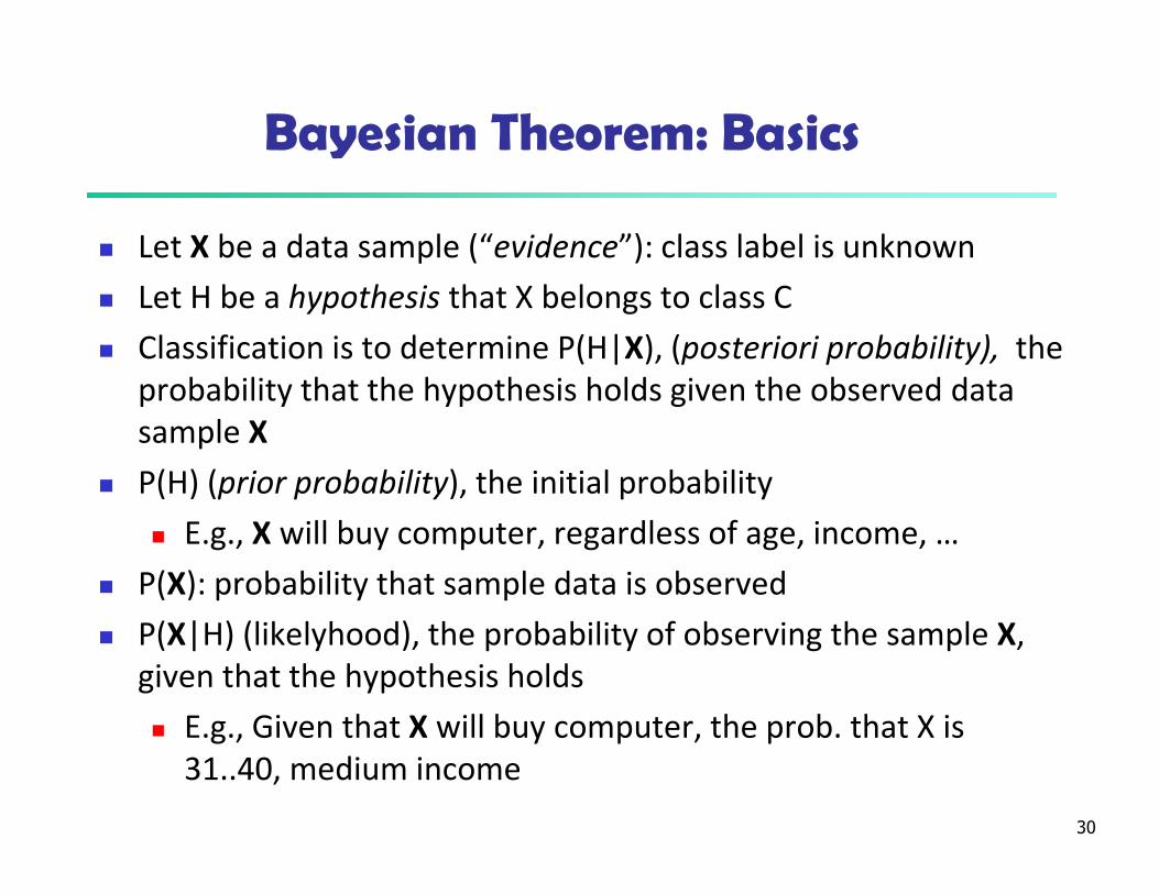
Bayesian Theorem: Basics
� Let X be a data sample (“evidence”): class label is unknown
� Let H be a hypothesis that X belongs to class C
� Classification is to determine P(H|X), (posteriori probability), the
probability that the hypothesis holds given the observed data
sample X
� P(H) (prior probability), the initial probability
� E.g., X will buy computer, regardless of age, income, …
� P(X): probability that sample data is observed
� P(X|H) (likelyhood), the probability of observing the sample X,
given that the hypothesis holds
� E.g., Given that X will buy computer, the prob. that X is
31..40, medium income
31
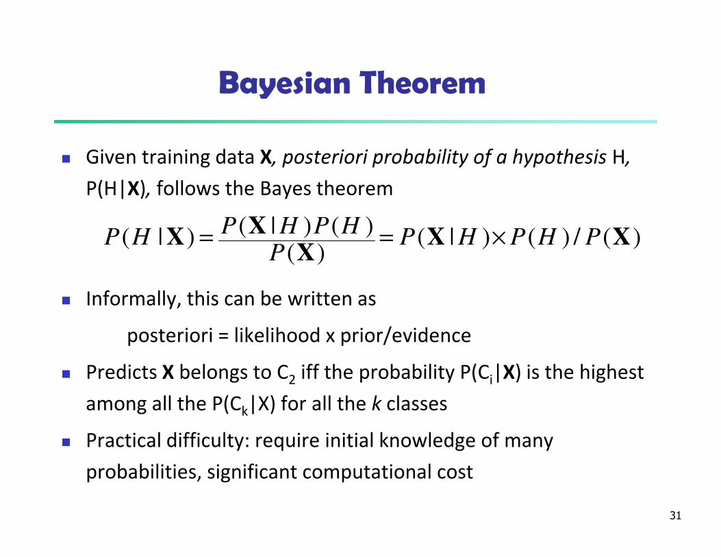
Bayesian Theorem
� Given training data X, posteriori probability of a hypothesis H,
P(H|X), follows the Bayes theorem
� Informally, this can be written as
posteriori = likelihood x prior/evidence
� Predicts X belongs to C2 iff the probability P(Ci|X) is the highest
among all the P(Ck|X) for all the k classes
� Practical difficulty: require initial knowledge of many
probabilities, significant computational cost
)(/)()|()(
)()|()|( XXX
XX PHPHPP
HPHPHP ×==
32
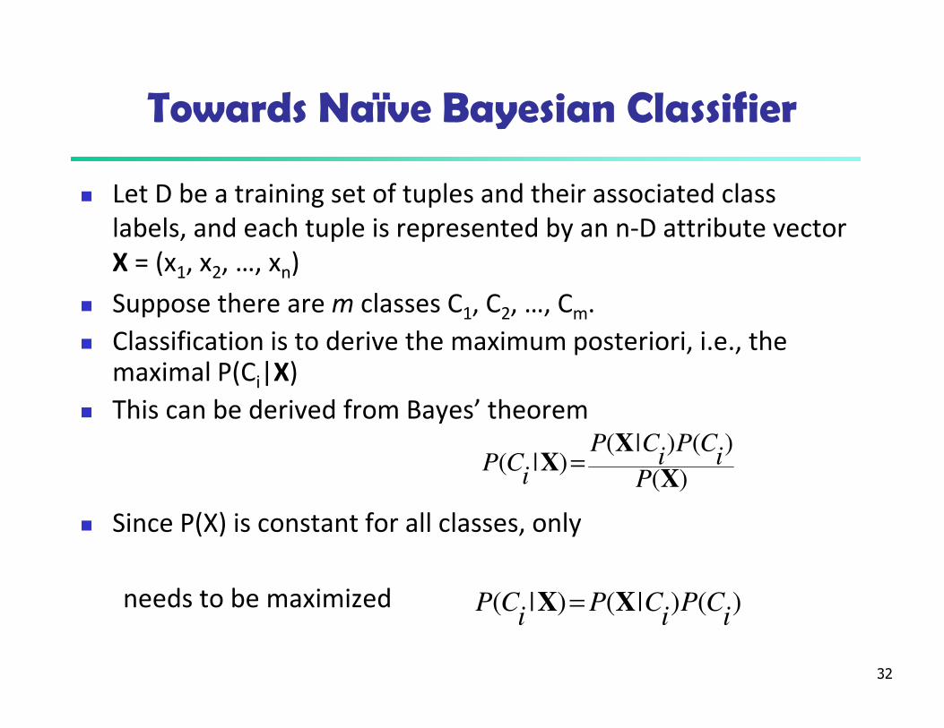
Towards Naïve Bayesian Classifier
� Let D be a training set of tuples and their associated class
labels, and each tuple is represented by an n-D attribute vector
X = (x1, x2, …, xn)
� Suppose there are m classes C1, C2, …, Cm.
� Classification is to derive the maximum posteriori, i.e., the maximal P(Ci|X)
� This can be derived from Bayes’ theorem
� Since P(X) is constant for all classes, only
needs to be maximized
)(
)()|()|(
X
XX
Pi
CPi
CP
iCP =
)()|()|(i
CPi
CPi
CP XX =
33
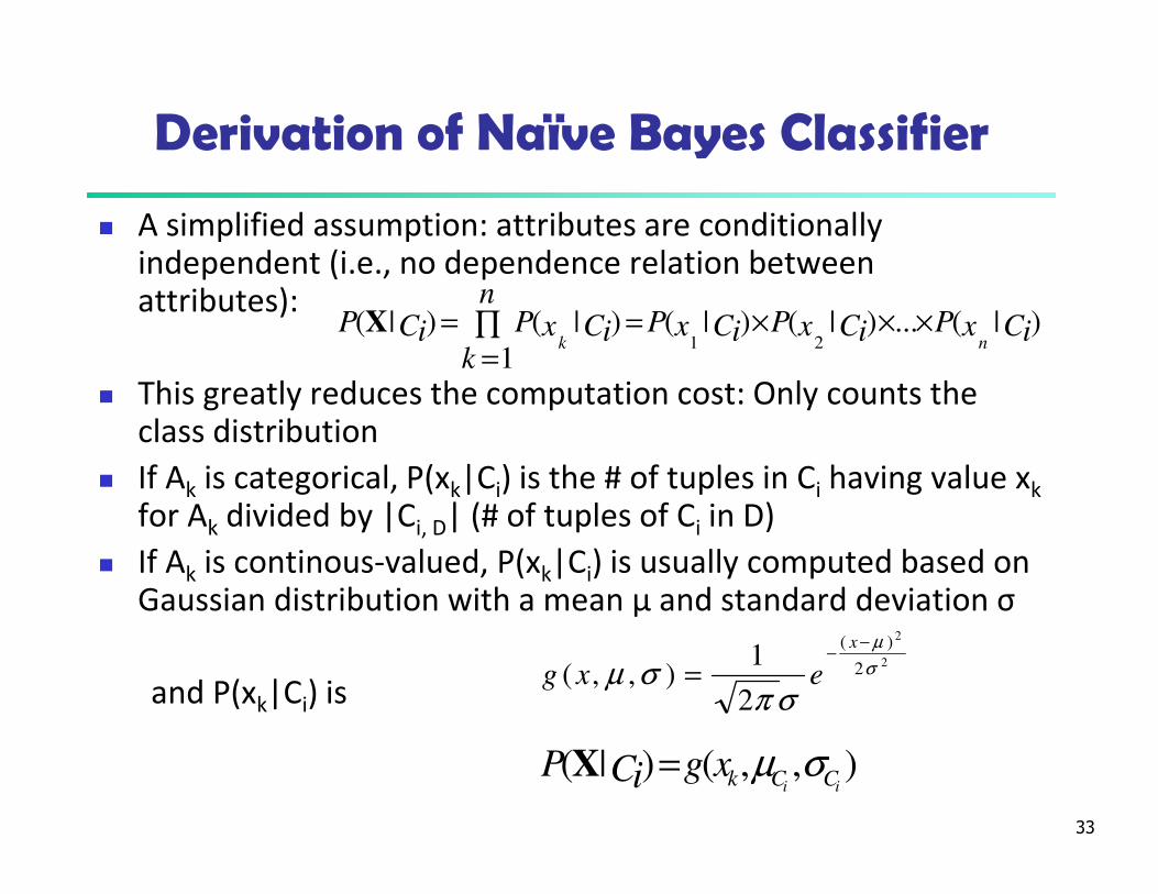
Derivation of Naïve Bayes Classifier
� A simplified assumption: attributes are conditionally independent (i.e., no dependence relation between attributes):
� This greatly reduces the computation cost: Only counts the class distribution
� If Ak is categorical, P(xk|Ci) is the # of tuples in Ci having value xk
for Ak divided by |Ci, D| (# of tuples of Ci in D)
� If Ak is continous-valued, P(xk|Ci) is usually computed based on Gaussian distribution with a mean μ and standard deviation σ
and P(xk|Ci) is
)|(...)|()|(
1
)|()|(21
CixPCixPCixPn
kCixPCiP
nk×××=∏
==X
2
2
2
)(
2
1),,( σ
µ
σπσµ
−−
=x
exg
),,()|(ii CCkxgCiP σµ=X
34
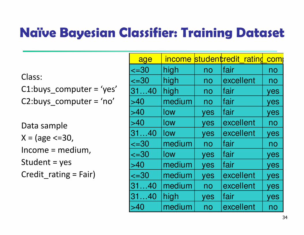
Naïve Bayesian Classifier: Training Dataset
Class:
C1:buys_computer = ‘yes’
C2:buys_computer = ‘no’
Data sample
X = (age <=30,
Income = medium,
Student = yes
Credit_rating = Fair)
age income studentcredit_ratings_comp
<=30 high no fair no
<=30 high no excellent no
31…40 high no fair yes
>40 medium no fair yes
>40 low yes fair yes
>40 low yes excellent no
31…40 low yes excellent yes
<=30 medium no fair no
<=30 low yes fair yes
>40 medium yes fair yes
<=30 medium yes excellent yes
31…40 medium no excellent yes
31…40 high yes fair yes
>40 medium no excellent no

35
Naïve Bayesian Classifier: An Example
� P(Ci): P(buys_computer = “yes”) = 9/14 = 0.643
P(buys_computer = “no”) = 5/14= 0.357
� Compute P(X|Ci) for each class
P(age = “<=30” | buys_computer = “yes”) = 2/9 = 0.222
P(age = “<= 30” | buys_computer = “no”) = 3/5 = 0.6
P(income = “medium” | buys_computer = “yes”) = 4/9 = 0.444
P(income = “medium” | buys_computer = “no”) = 2/5 = 0.4
P(student = “yes” | buys_computer = “yes) = 6/9 = 0.667
P(student = “yes” | buys_computer = “no”) = 1/5 = 0.2
P(credit_rating = “fair” | buys_computer = “yes”) = 6/9 = 0.667
P(credit_rating = “fair” | buys_computer = “no”) = 2/5 = 0.4
� X = (age <= 30 , income = medium, student = yes, credit_rating = fair)
P(X|Ci) : P(X|buys_computer = “yes”) = 0.222 x 0.444 x 0.667 x 0.667 = 0.044
P(X|buys_computer = “no”) = 0.6 x 0.4 x 0.2 x 0.4 = 0.019
P(X|Ci)*P(Ci) : P(X|buys_computer = “yes”) * P(buys_computer = “yes”) = 0.028
P(X|buys_computer = “no”) * P(buys_computer = “no”) = 0.007
Therefore, X belongs to class (“buys_computer = yes”)
36
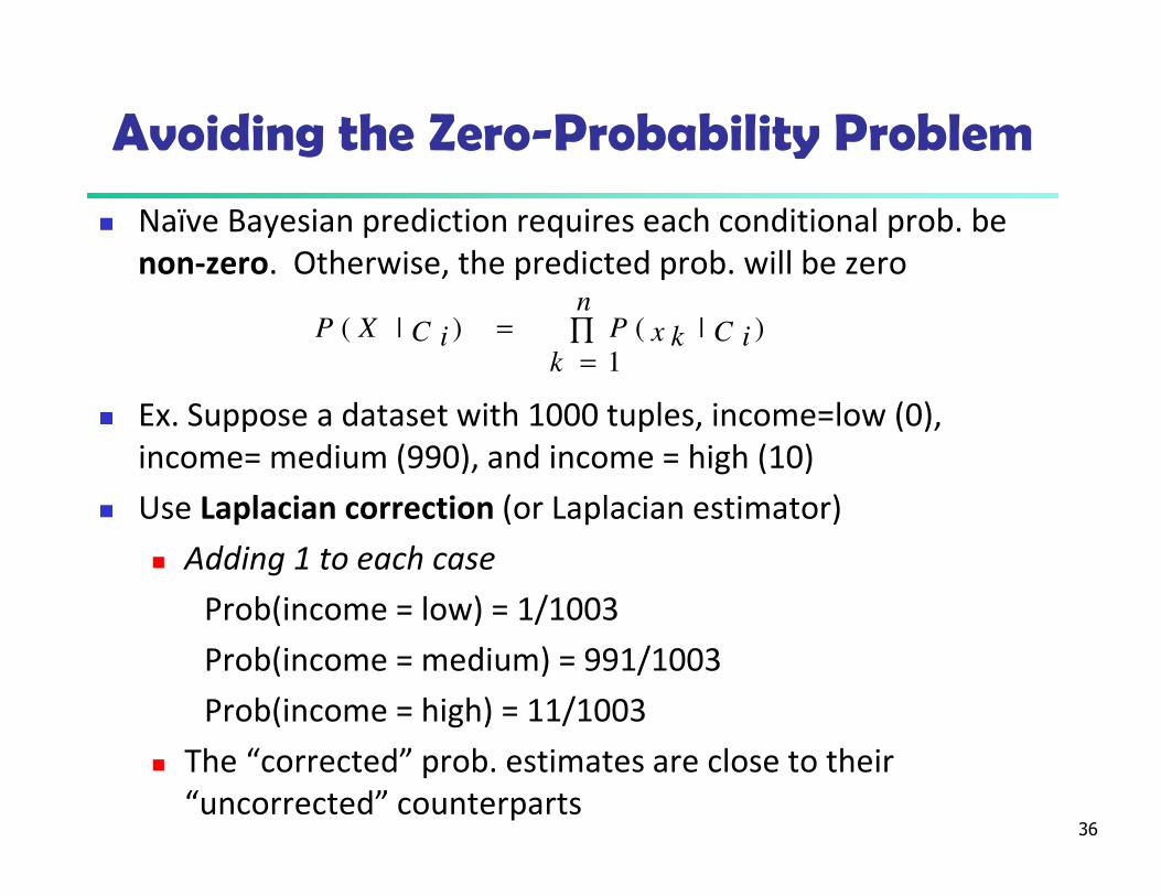
Avoiding the Zero-Probability Problem
� Naïve Bayesian prediction requires each conditional prob. be
non-zero. Otherwise, the predicted prob. will be zero
� Ex. Suppose a dataset with 1000 tuples, income=low (0),
income= medium (990), and income = high (10)
� Use Laplacian correction (or Laplacian estimator)
� Adding 1 to each case
Prob(income = low) = 1/1003
Prob(income = medium) = 991/1003
Prob(income = high) = 11/1003
� The “corrected” prob. estimates are close to their
“uncorrected” counterparts
∏=
=n
kC ix kPC iXP
1
)|()|(
37
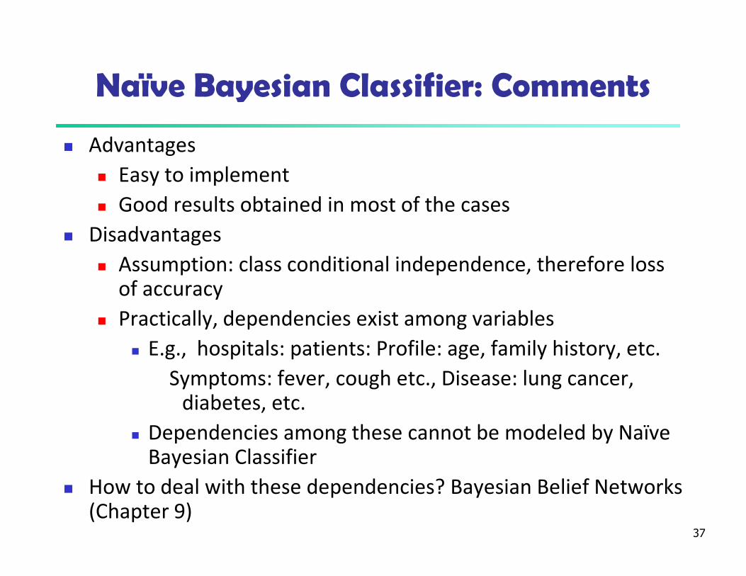
Naïve Bayesian Classifier: Comments
� Advantages
� Easy to implement
� Good results obtained in most of the cases
� Disadvantages
� Assumption: class conditional independence, therefore loss of accuracy
� Practically, dependencies exist among variables
� E.g., hospitals: patients: Profile: age, family history, etc.
Symptoms: fever, cough etc., Disease: lung cancer, diabetes, etc.
� Dependencies among these cannot be modeled by Naïve Bayesian Classifier
� How to deal with these dependencies? Bayesian Belief Networks (Chapter 9)
38
Chapter 8. Classification: Basic Concepts
� Classification: Basic Concepts
� Decision Tree Induction
� Bayes Classification Methods
� Rule-Based Classification
� Model Evaluation and Selection
� Techniques to Improve Classification Accuracy:
Ensemble Methods
� Summary

39
Using IF-THEN Rules for Classification
� Represent the knowledge in the form of IF-THEN rules
R: IF age = youth AND student = yes THEN buys_computer = yes
� Rule antecedent/precondition vs. rule consequent
� Assessment of a rule: coverage and accuracy
� ncovers = # of tuples covered by R
� ncorrect = # of tuples correctly classified by R
coverage(R) = ncovers /|D| /* D: training data set */
accuracy(R) = ncorrect / ncovers
� If more than one rule are triggered, need conflict resolution
� Size ordering: assign the highest priority to the triggering rules that has
the “toughest” requirement (i.e., with the most attribute tests)
� Class-based ordering: decreasing order of prevalence or misclassification
cost per class
� Rule-based ordering (decision list): rules are organized into one long
priority list, according to some measure of rule quality or by experts
40
age?
student? credit rating?
<=30 >40
no yes yes
yes
31..40
fairexcellentyesno
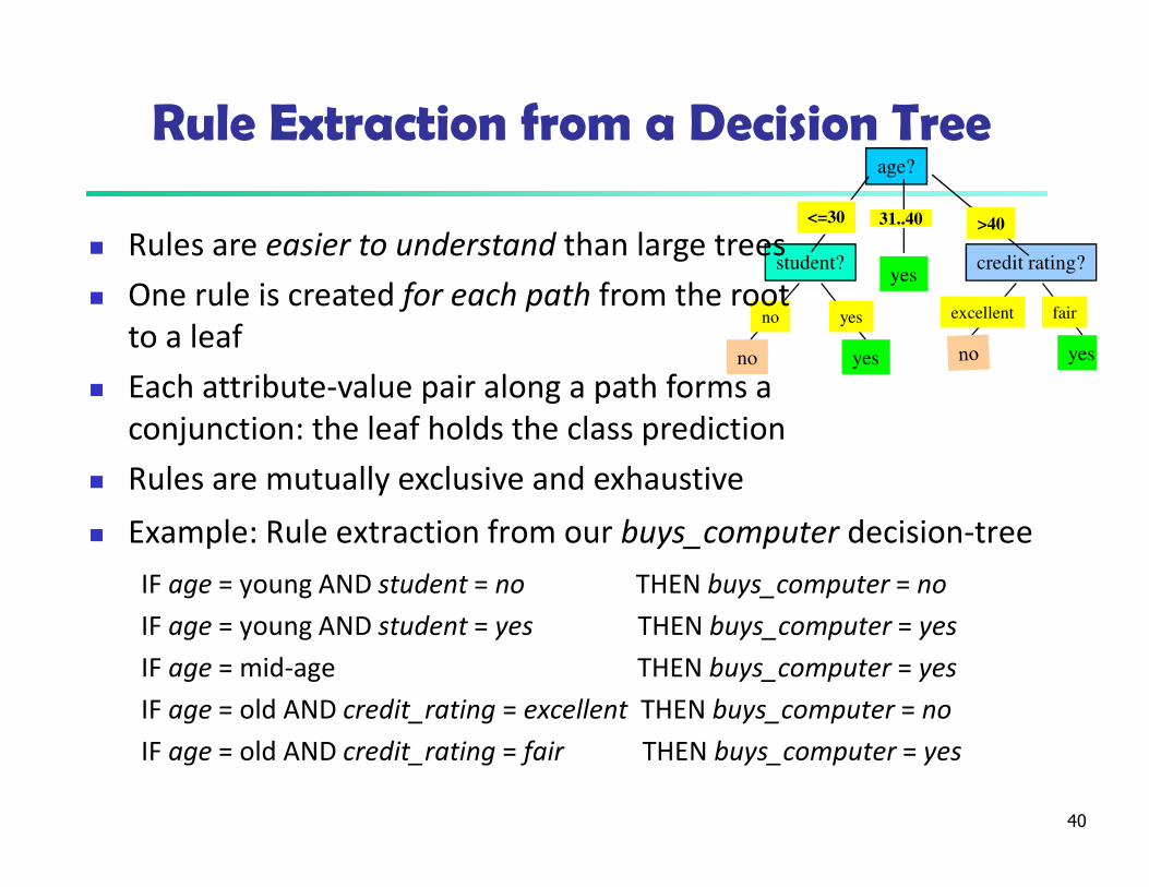
� Example: Rule extraction from our buys_computer decision-tree
IF age = young AND student = no THEN buys_computer = no
IF age = young AND student = yes THEN buys_computer = yes
IF age = mid-age THEN buys_computer = yes
IF age = old AND credit_rating = excellent THEN buys_computer = no
IF age = old AND credit_rating = fair THEN buys_computer = yes
Rule Extraction from a Decision Tree
� Rules are easier to understand than large trees
� One rule is created for each path from the root
to a leaf
� Each attribute-value pair along a path forms a
conjunction: the leaf holds the class prediction
� Rules are mutually exclusive and exhaustive
41
Rule Induction: Sequential Covering Method
� Sequential covering algorithm: Extracts rules directly from training data
� Typical sequential covering algorithms: FOIL, AQ, CN2, RIPPER
� Rules are learned sequentially, each for a given class Ci will cover many tuples of Ci but none (or few) of the tuples of other classes
� Steps:
� Rules are learned one at a time
� Each time a rule is learned, the tuples covered by the rules are removed
� The process repeats on the remaining tuples unless termination condition, e.g., when no more training examples or when the quality of a rule returned is below a user-specified threshold
� Comp. w. decision-tree induction: learning a set of rules simultaneously
42
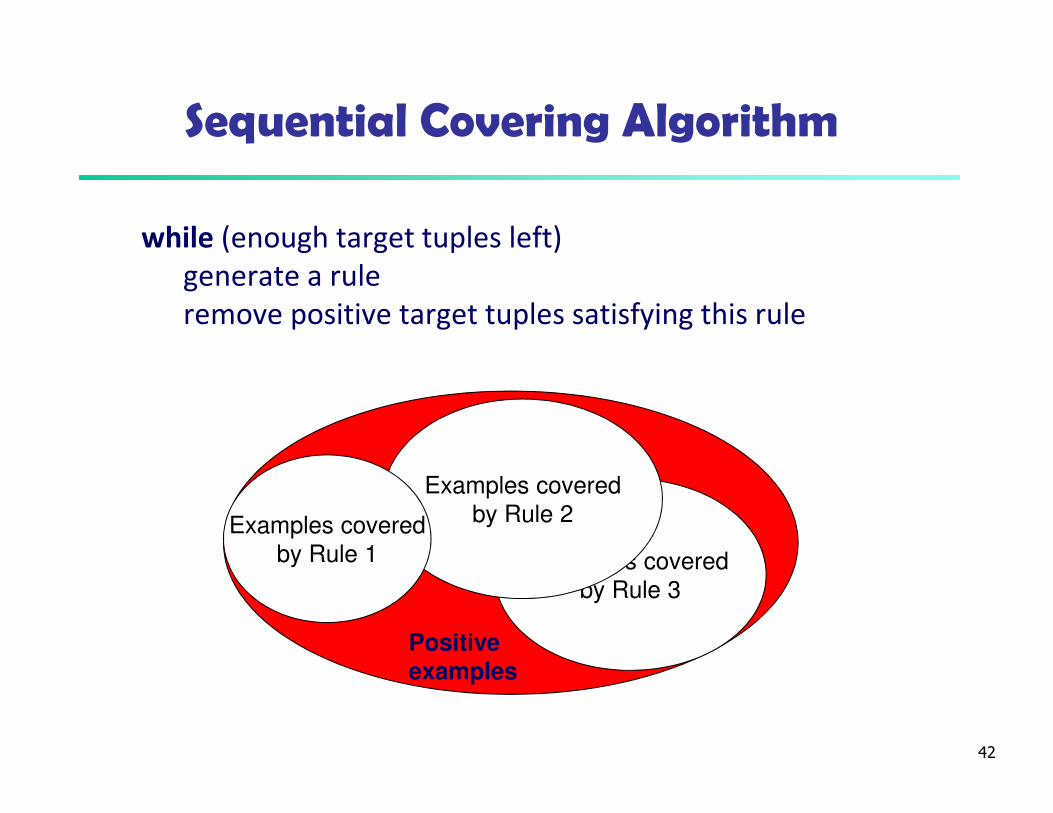
Sequential Covering Algorithm
while (enough target tuples left)
generate a rule
remove positive target tuples satisfying this rule
Examples covered
by Rule 3
Examples covered
by Rule 2Examples covered
by Rule 1
Positive
examples
43
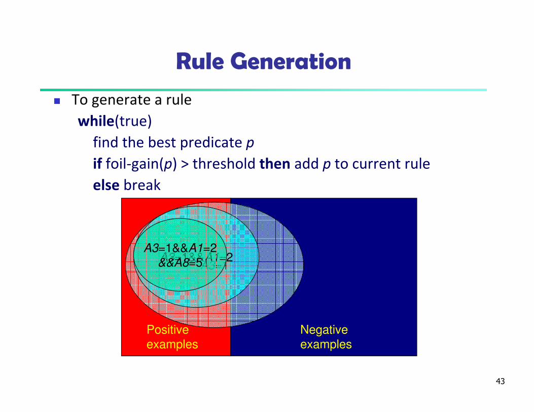
Rule Generation
� To generate a rule
while(true)
find the best predicate p
if foil-gain(p) > threshold then add p to current rule
else break
Positive
examples
Negative
examples
A3=1A3=1&&A1=2
A3=1&&A1=2
&&A8=5
44
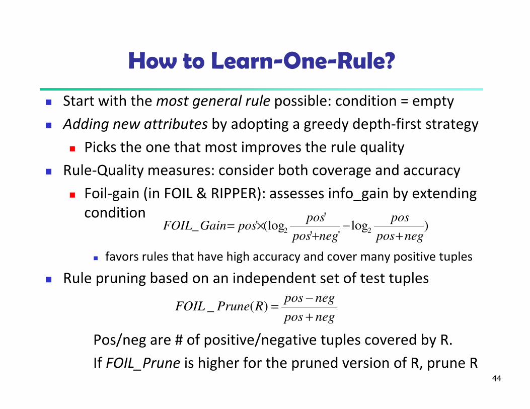
How to Learn-One-Rule?
� Start with the most general rule possible: condition = empty
� Adding new attributes by adopting a greedy depth-first strategy
� Picks the one that most improves the rule quality
� Rule-Quality measures: consider both coverage and accuracy
� Foil-gain (in FOIL & RIPPER): assesses info_gain by extending
condition
� favors rules that have high accuracy and cover many positive tuples
� Rule pruning based on an independent set of test tuples
Pos/neg are # of positive/negative tuples covered by R.
If FOIL_Prune is higher for the pruned version of R, prune R
)log''
'(log'_ 22
negpos
pos
negpos
posposGainFOIL
+−
+×=
negpos
negposRPruneFOIL
+
−=)(_
45
Chapter 8. Classification: Basic Concepts
� Classification: Basic Concepts
� Decision Tree Induction
� Bayes Classification Methods
� Rule-Based Classification
� Model Evaluation and Selection
� Techniques to Improve Classification Accuracy:
Ensemble Methods
� Summary
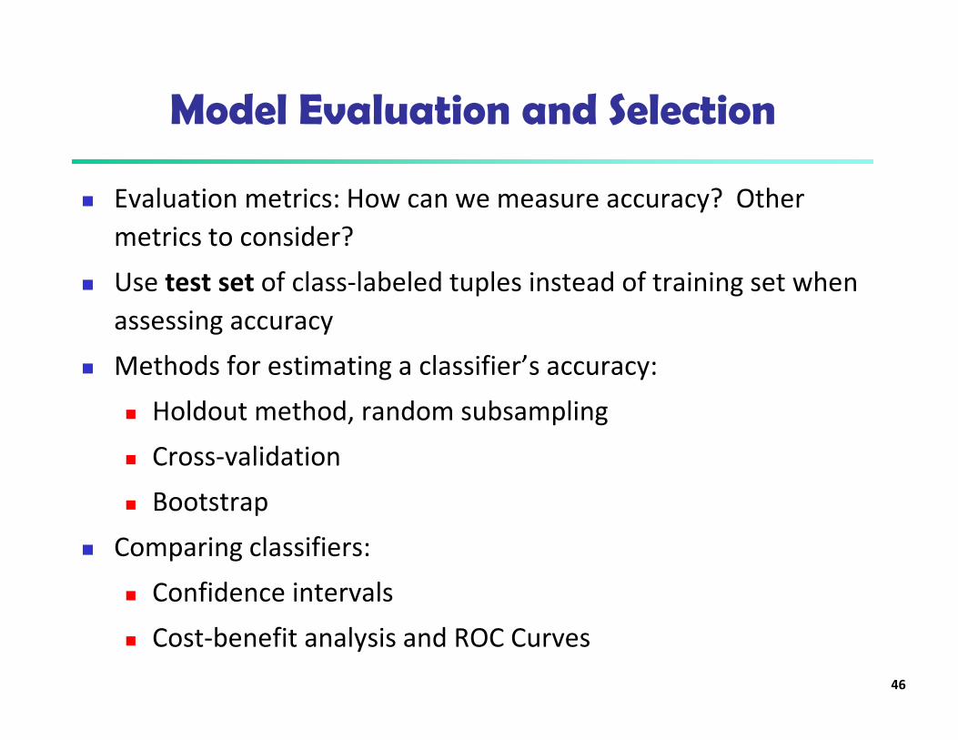
Model Evaluation and Selection
� Evaluation metrics: How can we measure accuracy? Other
metrics to consider?
� Use test set of class-labeled tuples instead of training set when
assessing accuracy
� Methods for estimating a classifier’s accuracy:
� Holdout method, random subsampling
� Cross-validation
� Bootstrap
� Comparing classifiers:
� Confidence intervals
� Cost-benefit analysis and ROC Curves
46
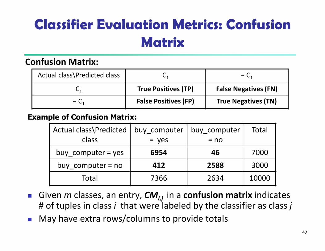
Classifier Evaluation Metrics: Confusion Matrix
Actual class\Predicted
class
buy_computer
= yes
buy_computer
= no
Total
buy_computer = yes 6954 46 7000
buy_computer = no 412 2588 3000
Total 7366 2634 10000
� Given m classes, an entry, CMi,j in a confusion matrix indicates # of tuples in class i that were labeled by the classifier as class j
� May have extra rows/columns to provide totals
Confusion Matrix:
Actual class\Predicted class C1 ¬ C1
C1 True Positives (TP) False Negatives (FN)
¬ C1 False Positives (FP) True Negatives (TN)
Example of Confusion Matrix:
47

Classifier Evaluation Metrics: Accuracy, Error Rate, Sensitivity and Specificity
� Classifier Accuracy, or
recognition rate: percentage of
test set tuples that are correctly
classified
Accuracy = (TP + TN)/All
� Error rate: 1 – accuracy, or
Error rate = (FP + FN)/All
� Class Imbalance Problem:
� One class may be rare, e.g.
fraud, or HIV-positive
� Significant majority of the
negative class and minority of
the positive class
� Sensitivity: True Positive
recognition rate
� Sensitivity = TP/P
� Specificity: True Negative
recognition rate
� Specificity = TN/N
A\P C ¬C
C TP FN P
¬C FP TN N
P’ N’ All
48
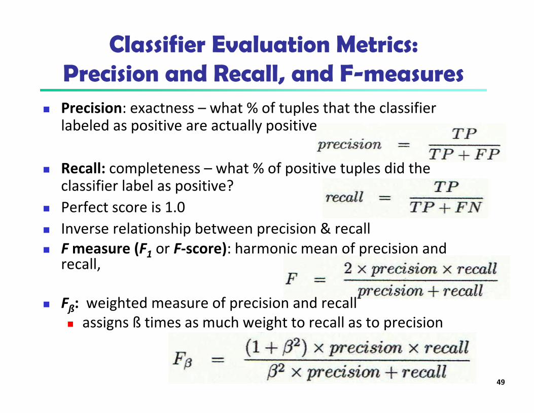
Classifier Evaluation Metrics: Precision and Recall, and F-measures
� Precision: exactness – what % of tuples that the classifier labeled as positive are actually positive
� Recall: completeness – what % of positive tuples did the classifier label as positive?
� Perfect score is 1.0
� Inverse relationship between precision & recall
� F measure (F1 or F-score): harmonic mean of precision and recall,
� Fß: weighted measure of precision and recall
� assigns ß times as much weight to recall as to precision
49
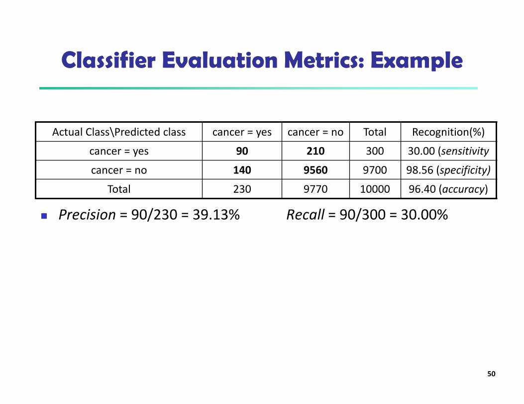
Classifier Evaluation Metrics: Example
50
� Precision = 90/230 = 39.13% Recall = 90/300 = 30.00%
Actual Class\Predicted class cancer = yes cancer = no Total Recognition(%)
cancer = yes 90 210 300 30.00 (sensitivity
cancer = no 140 9560 9700 98.56 (specificity)
Total 230 9770 10000 96.40 (accuracy)

Evaluating Classifier Accuracy:Holdout & Cross-Validation Methods
� Holdout method
� Given data is randomly partitioned into two independent sets
� Training set (e.g., 2/3) for model construction
� Test set (e.g., 1/3) for accuracy estimation
� Random sampling: a variation of holdout
� Repeat holdout k times, accuracy = avg. of the accuracies obtained
� Cross-validation (k-fold, where k = 10 is most popular)
� Randomly partition the data into k mutually exclusive subsets, each approximately equal size
� At i-th iteration, use Di as test set and others as training set
� Leave-one-out: k folds where k = # of tuples, for small sized data
� *Stratified cross-validation*: folds are stratified so that class dist. in each fold is approx. the same as that in the initial data
51
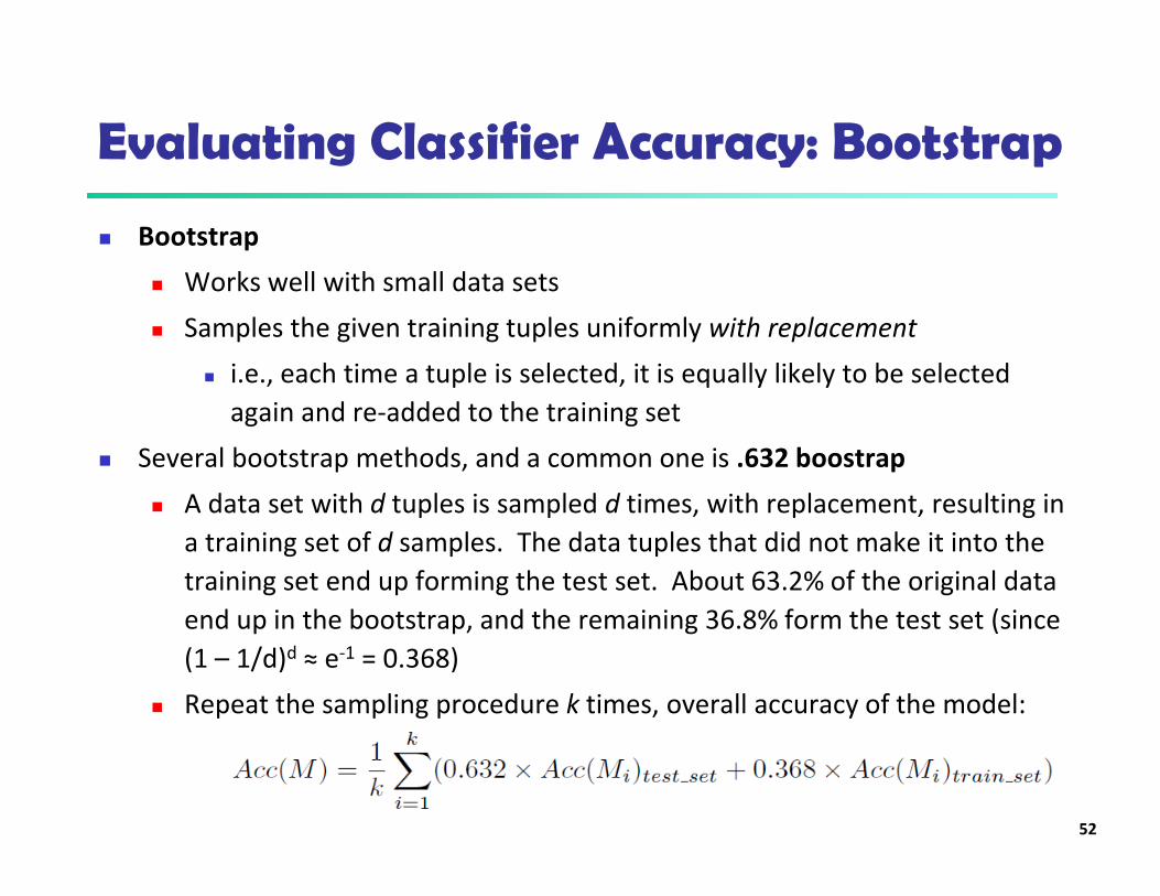
Evaluating Classifier Accuracy: Bootstrap
� Bootstrap
� Works well with small data sets
� Samples the given training tuples uniformly with replacement
� i.e., each time a tuple is selected, it is equally likely to be selected
again and re-added to the training set
� Several bootstrap methods, and a common one is .632 boostrap
� A data set with d tuples is sampled d times, with replacement, resulting in
a training set of d samples. The data tuples that did not make it into the
training set end up forming the test set. About 63.2% of the original data
end up in the bootstrap, and the remaining 36.8% form the test set (since
(1 – 1/d)d ≈ e-1 = 0.368)
� Repeat the sampling procedure k times, overall accuracy of the model:
52

Estimating Confidence Intervals:Classifier Models M1 vs. M2
� Suppose we have 2 classifiers, M1 and M2, which one is better?
� Use 10-fold cross-validation to obtain and
� These mean error rates are just estimates of error on the true
population of future data cases
� What if the difference between the 2 error rates is just
attributed to chance?
� Use a test of statistical significance
� Obtain confidence limits for our error estimates
53
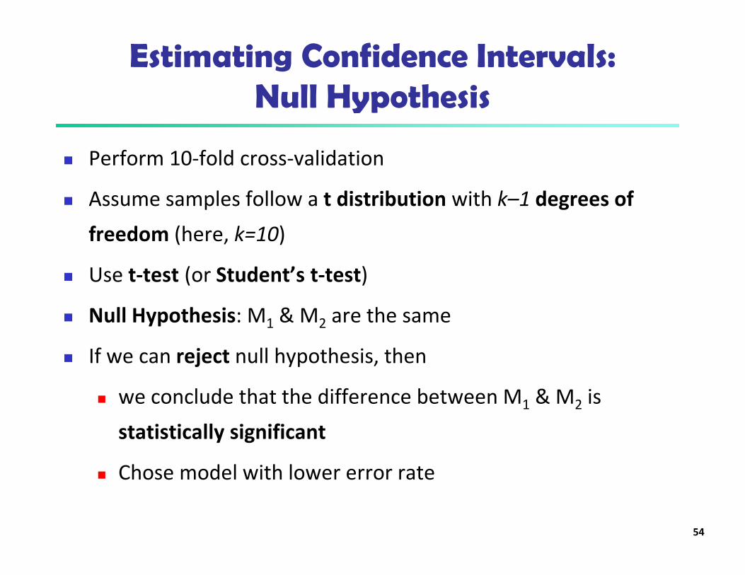
Estimating Confidence Intervals:Null Hypothesis
� Perform 10-fold cross-validation
� Assume samples follow a t distribution with k–1 degrees of
freedom (here, k=10)
� Use t-test (or Student’s t-test)
� Null Hypothesis: M1 & M2 are the same
� If we can reject null hypothesis, then
� we conclude that the difference between M1 & M2 is
statistically significant
� Chose model with lower error rate
54
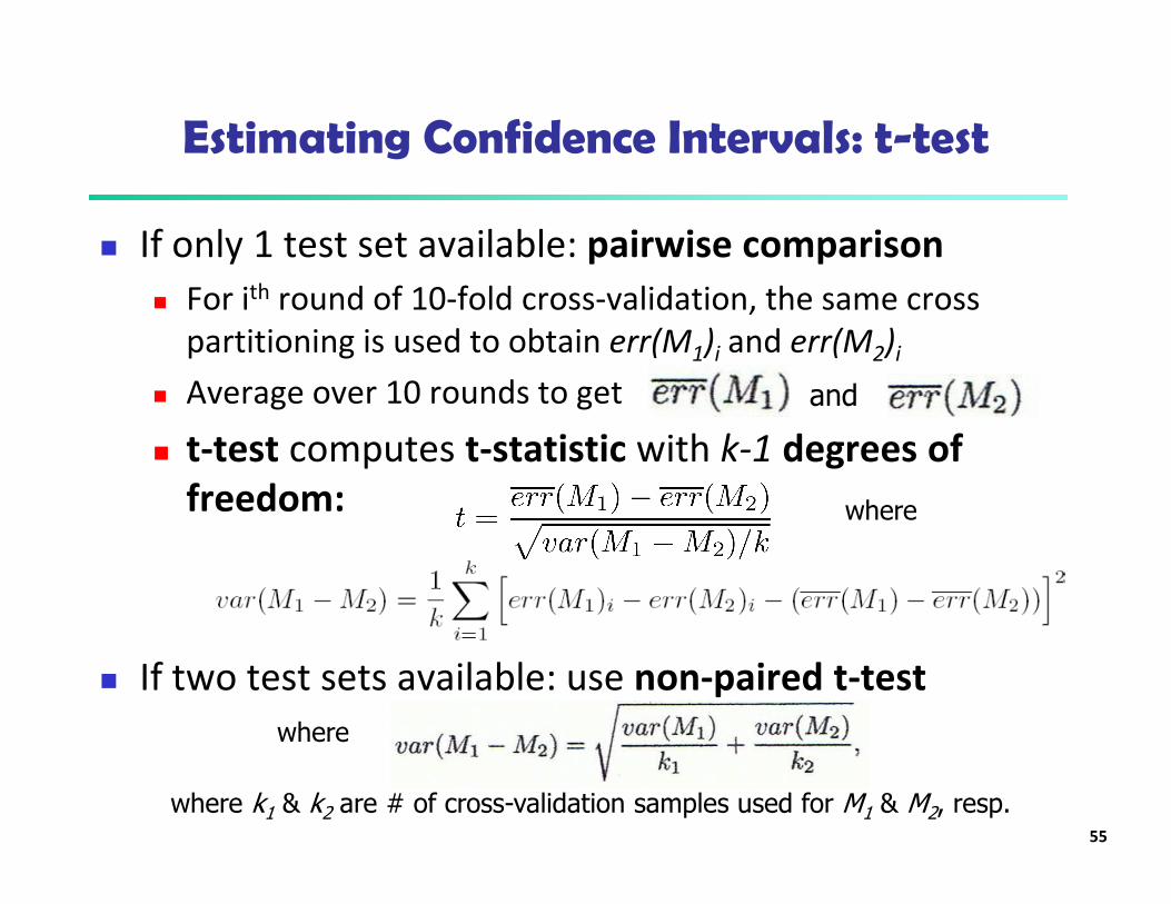
Estimating Confidence Intervals: t-test
� If only 1 test set available: pairwise comparison
� For ith round of 10-fold cross-validation, the same cross
partitioning is used to obtain err(M1)i and err(M2)i
� Average over 10 rounds to get
� t-test computes t-statistic with k-1 degrees of
freedom:
� If two test sets available: use non-paired t-test
where
and
where
where k1 & k2 are # of cross-validation samples used for M1 & M2, resp.55
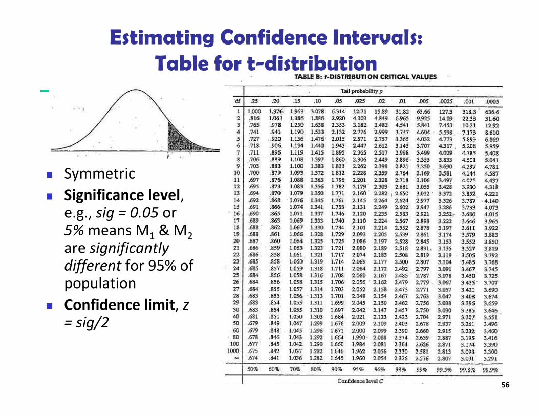
Estimating Confidence Intervals:Table for t-distribution
� Symmetric
� Significance level, e.g., sig = 0.05 or5% means M1 & M2
are significantly different for 95% of population
� Confidence limit, z = sig/2
56
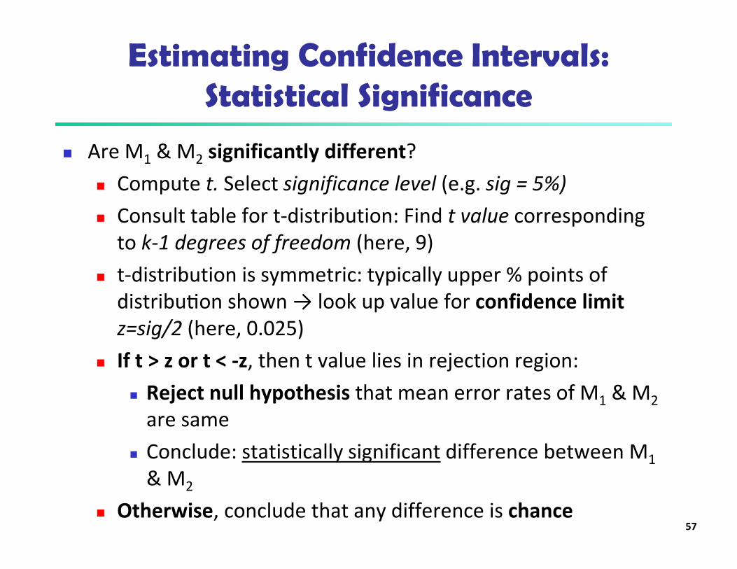
Estimating Confidence Intervals:Statistical Significance
� Are M1 & M2 significantly different?
� Compute t. Select significance level (e.g. sig = 5%)
� Consult table for t-distribution: Find t value corresponding
to k-1 degrees of freedom (here, 9)
� t-distribution is symmetric: typically upper % points of
distribueon shown → look up value for confidence limit
z=sig/2 (here, 0.025)
� If t > z or t < -z, then t value lies in rejection region:
� Reject null hypothesis that mean error rates of M1 & M2
are same
� Conclude: statistically significant difference between M1
& M2
� Otherwise, conclude that any difference is chance57

Model Selection: ROC Curves
� ROC (Receiver Operating Characteristics) curves: for visual comparison of classification models
� Originated from signal detection theory
� Shows the trade-off between the true positive rate and the false positive rate
� The area under the ROC curve is a measure of the accuracy of the model
� Rank the test tuples in decreasing order: the one that is most likely to belong to the positive class appears at the top of the list
� The closer to the diagonal line (i.e., the closer the area is to 0.5), the less accurate is the model
� Vertical axis represents the true positive rate
� Horizontal axis rep. the false positive rate
� The plot also shows a diagonal line
� A model with perfect accuracy will have an area of 1.0
58
Issues Affecting Model Selection
� Accuracy
� classifier accuracy: predicting class label
� Speed
� time to construct the model (training time)
� time to use the model (classification/prediction time)
� Robustness: handling noise and missing values
� Scalability: efficiency in disk-resident databases
� Interpretability
� understanding and insight provided by the model
� Other measures, e.g., goodness of rules, such as decision tree
size or compactness of classification rules
59
60
Chapter 8. Classification: Basic Concepts
� Classification: Basic Concepts
� Decision Tree Induction
� Bayes Classification Methods
� Rule-Based Classification
� Model Evaluation and Selection
� Techniques to Improve Classification Accuracy:
Ensemble Methods
� Summary

Ensemble Methods: Increasing the Accuracy
� Ensemble methods
� Use a combination of models to increase accuracy
� Combine a series of k learned models, M1, M2, …, Mk, with
the aim of creating an improved model M*
� Popular ensemble methods
� Bagging: averaging the prediction over a collection of
classifiers
� Boosting: weighted vote with a collection of classifiers
� Ensemble: combining a set of heterogeneous classifiers
61

Bagging: Boostrap Aggregation
� Analogy: Diagnosis based on multiple doctors’ majority vote
� Training
� Given a set D of d tuples, at each iteration i, a training set Di of d tuples
is sampled with replacement from D (i.e., bootstrap)
� A classifier model Mi is learned for each training set Di
� Classification: classify an unknown sample X
� Each classifier Mi returns its class prediction
� The bagged classifier M* counts the votes and assigns the class with the
most votes to X
� Prediction: can be applied to the prediction of continuous values by taking
the average value of each prediction for a given test tuple
� Accuracy
� Often significantly better than a single classifier derived from D
� For noise data: not considerably worse, more robust
� Proved improved accuracy in prediction62
Boosting
� Analogy: Consult several doctors, based on a combination of weighted diagnoses—weight assigned based on the previous diagnosis accuracy
� How boosting works?
� Weights are assigned to each training tuple
� A series of k classifiers is iteratively learned
� After a classifier Mi is learned, the weights are updated to allow the subsequent classifier, Mi+1, to pay more attention to the training tuples that were misclassified by Mi
� The final M* combines the votes of each individual classifier, where the weight of each classifier's vote is a function of its accuracy
� Boosting algorithm can be extended for numeric prediction
� Comparing with bagging: Boosting tends to have greater accuracy, but it also risks overfitting the model to misclassified data
63
64
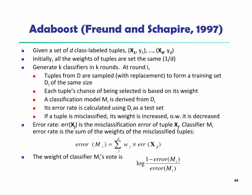
Adaboost (Freund and Schapire, 1997)
� Given a set of d class-labeled tuples, (X1, y1), …, (Xd, yd)
� Initially, all the weights of tuples are set the same (1/d)
� Generate k classifiers in k rounds. At round i,
� Tuples from D are sampled (with replacement) to form a training set Di of the same size
� Each tuple’s chance of being selected is based on its weight
� A classification model Mi is derived from Di
� Its error rate is calculated using Di as a test set
� If a tuple is misclassified, its weight is increased, o.w. it is decreased
� Error rate: err(Xj) is the misclassification error of tuple Xj. Classifier Mi
error rate is the sum of the weights of the misclassified tuples:
� The weight of classifier Mi’s vote is
)(
)(1log
i
i
Merror
Merror−
∑ ×=d
j
ji errwMerror )()( jX
Random Forest (Breiman 2001)
� Random Forest:
� Each classifier in the ensemble is a decision tree classifier and is
generated using a random selection of attributes at each node to
determine the split
� During classification, each tree votes and the most popular class is
returned
� Two Methods to construct Random Forest:
� Forest-RI (random input selection): Randomly select, at each node, F
attributes as candidates for the split at the node. The CART methodology
is used to grow the trees to maximum size
� Forest-RC (random linear combinations): Creates new attributes (or
features) that are a linear combination of the existing attributes
(reduces the correlation between individual classifiers)
� Comparable in accuracy to Adaboost, but more robust to errors and outliers
� Insensitive to the number of attributes selected for consideration at each
split, and faster than bagging or boosting65

Classification of Class-Imbalanced Data Sets
� Class-imbalance problem: Rare positive example but numerous negative ones, e.g., medical diagnosis, fraud, oil-spill, fault, etc.
� Traditional methods assume a balanced distribution of classes and equal error costs: not suitable for class-imbalanced data
� Typical methods for imbalance data in 2-class classification:
� Oversampling: re-sampling of data from positive class
� Under-sampling: randomly eliminate tuples from negative class
� Threshold-moving: moves the decision threshold, t, so that the rare class tuples are easier to classify, and hence, less chance of costly false negative errors
� Ensemble techniques: Ensemble multiple classifiers introduced above
� Still difficult for class imbalance problem on multiclass tasks
66

67
Chapter 8. Classification: Basic Concepts
� Classification: Basic Concepts
� Decision Tree Induction
� Bayes Classification Methods
� Rule-Based Classification
� Model Evaluation and Selection
� Techniques to Improve Classification Accuracy:
Ensemble Methods
� Summary

Summary (I)
� Classification is a form of data analysis that extracts models
describing important data classes.
� Effective and scalable methods have been developed for decision
tree induction, Naive Bayesian classification, rule-based
classification, and many other classification methods.
� Evaluation metrics include: accuracy, sensitivity, specificity,
precision, recall, F measure, and Fß measure.
� Stratified k-fold cross-validation is recommended for accuracy
estimation. Bagging and boosting can be used to increase overall
accuracy by learning and combining a series of individual models.
68

Summary (II)
� Significance tests and ROC curves are useful for model selection.
� There have been numerous comparisons of the different
classification methods; the matter remains a research topic
� No single method has been found to be superior over all others
for all data sets
� Issues such as accuracy, training time, robustness, scalability,
and interpretability must be considered and can involve trade-
offs, further complicating the quest for an overall superior
method
69
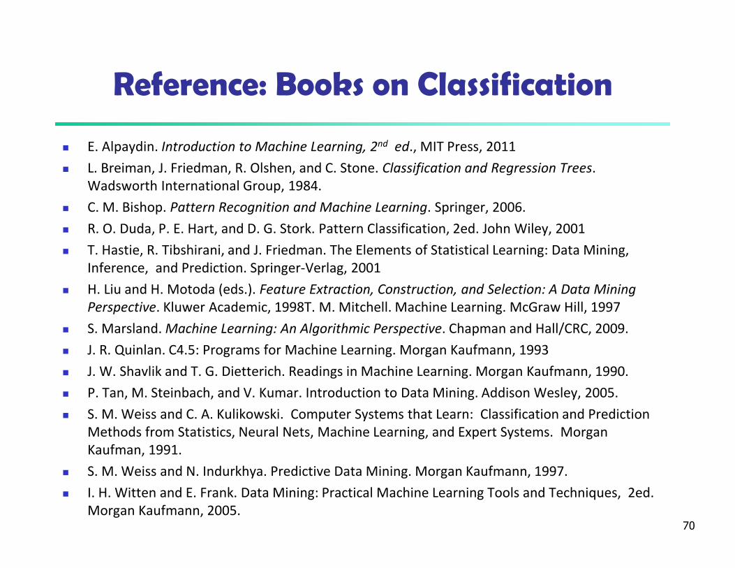
Reference: Books on Classification
� E. Alpaydin. Introduction to Machine Learning, 2nd ed., MIT Press, 2011
� L. Breiman, J. Friedman, R. Olshen, and C. Stone. Classification and Regression Trees.
Wadsworth International Group, 1984.
� C. M. Bishop. Pattern Recognition and Machine Learning. Springer, 2006.
� R. O. Duda, P. E. Hart, and D. G. Stork. Pattern Classification, 2ed. John Wiley, 2001
� T. Hastie, R. Tibshirani, and J. Friedman. The Elements of Statistical Learning: Data Mining,
Inference, and Prediction. Springer-Verlag, 2001
� H. Liu and H. Motoda (eds.). Feature Extraction, Construction, and Selection: A Data Mining
Perspective. Kluwer Academic, 1998T. M. Mitchell. Machine Learning. McGraw Hill, 1997
� S. Marsland. Machine Learning: An Algorithmic Perspective. Chapman and Hall/CRC, 2009.
� J. R. Quinlan. C4.5: Programs for Machine Learning. Morgan Kaufmann, 1993
� J. W. Shavlik and T. G. Dietterich. Readings in Machine Learning. Morgan Kaufmann, 1990.
� P. Tan, M. Steinbach, and V. Kumar. Introduction to Data Mining. Addison Wesley, 2005.
� S. M. Weiss and C. A. Kulikowski. Computer Systems that Learn: Classification and Prediction
Methods from Statistics, Neural Nets, Machine Learning, and Expert Systems. Morgan
Kaufman, 1991.
� S. M. Weiss and N. Indurkhya. Predictive Data Mining. Morgan Kaufmann, 1997.
� I. H. Witten and E. Frank. Data Mining: Practical Machine Learning Tools and Techniques, 2ed.
Morgan Kaufmann, 2005.70
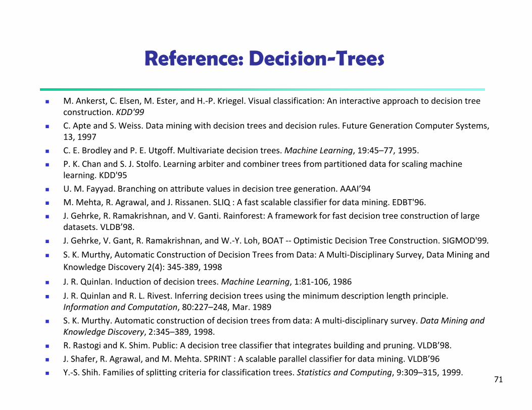
Reference: Decision-Trees
� M. Ankerst, C. Elsen, M. Ester, and H.-P. Kriegel. Visual classification: An interactive approach to decision tree
construction. KDD'99
� C. Apte and S. Weiss. Data mining with decision trees and decision rules. Future Generation Computer Systems,
13, 1997
� C. E. Brodley and P. E. Utgoff. Multivariate decision trees. Machine Learning, 19:45–77, 1995.
� P. K. Chan and S. J. Stolfo. Learning arbiter and combiner trees from partitioned data for scaling machine
learning. KDD'95
� U. M. Fayyad. Branching on attribute values in decision tree generation. AAAI’94
� M. Mehta, R. Agrawal, and J. Rissanen. SLIQ : A fast scalable classifier for data mining. EDBT'96.
� J. Gehrke, R. Ramakrishnan, and V. Ganti. Rainforest: A framework for fast decision tree construction of large
datasets. VLDB’98.
� J. Gehrke, V. Gant, R. Ramakrishnan, and W.-Y. Loh, BOAT -- Optimistic Decision Tree Construction. SIGMOD'99.
� S. K. Murthy, Automatic Construction of Decision Trees from Data: A Multi-Disciplinary Survey, Data Mining and
Knowledge Discovery 2(4): 345-389, 1998
� J. R. Quinlan. Induction of decision trees. Machine Learning, 1:81-106, 1986
� J. R. Quinlan and R. L. Rivest. Inferring decision trees using the minimum description length principle.
Information and Computation, 80:227–248, Mar. 1989
� S. K. Murthy. Automatic construction of decision trees from data: A multi-disciplinary survey. Data Mining and
Knowledge Discovery, 2:345–389, 1998.
� R. Rastogi and K. Shim. Public: A decision tree classifier that integrates building and pruning. VLDB’98.
� J. Shafer, R. Agrawal, and M. Mehta. SPRINT : A scalable parallel classifier for data mining. VLDB’96
� Y.-S. Shih. Families of splitting criteria for classification trees. Statistics and Computing, 9:309–315, 1999.71
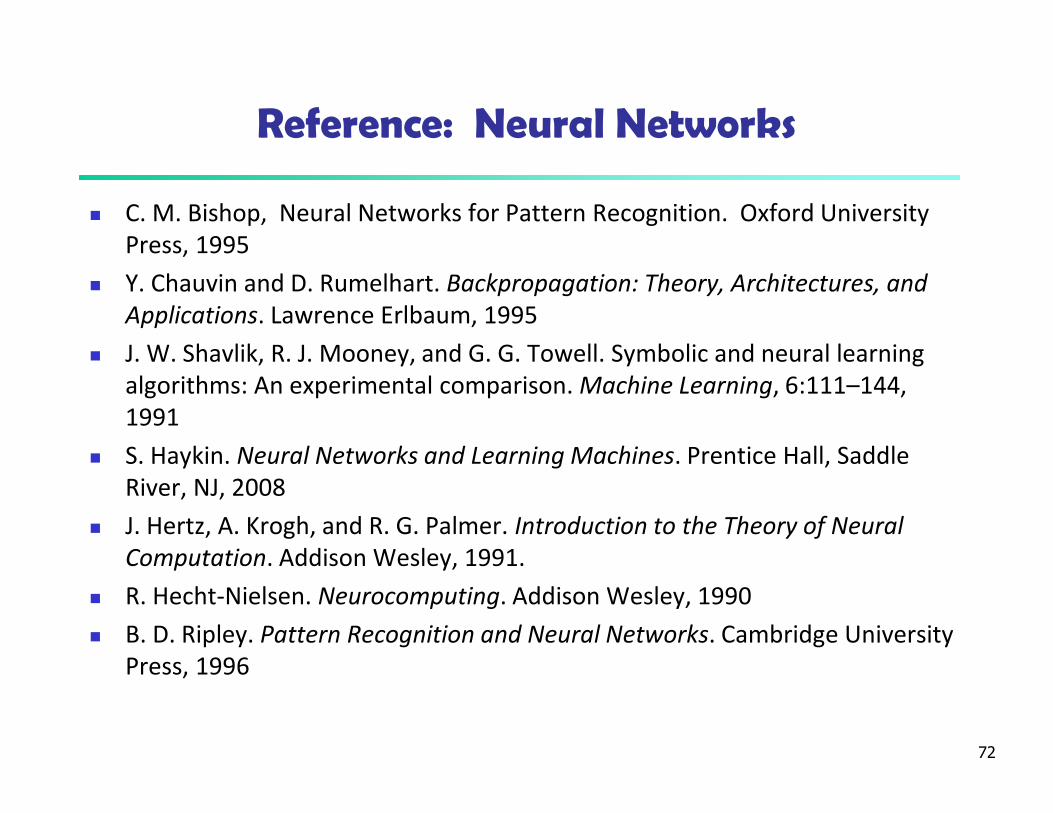
Reference: Neural Networks
� C. M. Bishop, Neural Networks for Pattern Recognition. Oxford University
Press, 1995
� Y. Chauvin and D. Rumelhart. Backpropagation: Theory, Architectures, and
Applications. Lawrence Erlbaum, 1995
� J. W. Shavlik, R. J. Mooney, and G. G. Towell. Symbolic and neural learning
algorithms: An experimental comparison. Machine Learning, 6:111–144,
1991
� S. Haykin. Neural Networks and Learning Machines. Prentice Hall, Saddle
River, NJ, 2008
� J. Hertz, A. Krogh, and R. G. Palmer. Introduction to the Theory of Neural
Computation. Addison Wesley, 1991.
� R. Hecht-Nielsen. Neurocomputing. Addison Wesley, 1990
� B. D. Ripley. Pattern Recognition and Neural Networks. Cambridge University
Press, 1996
72
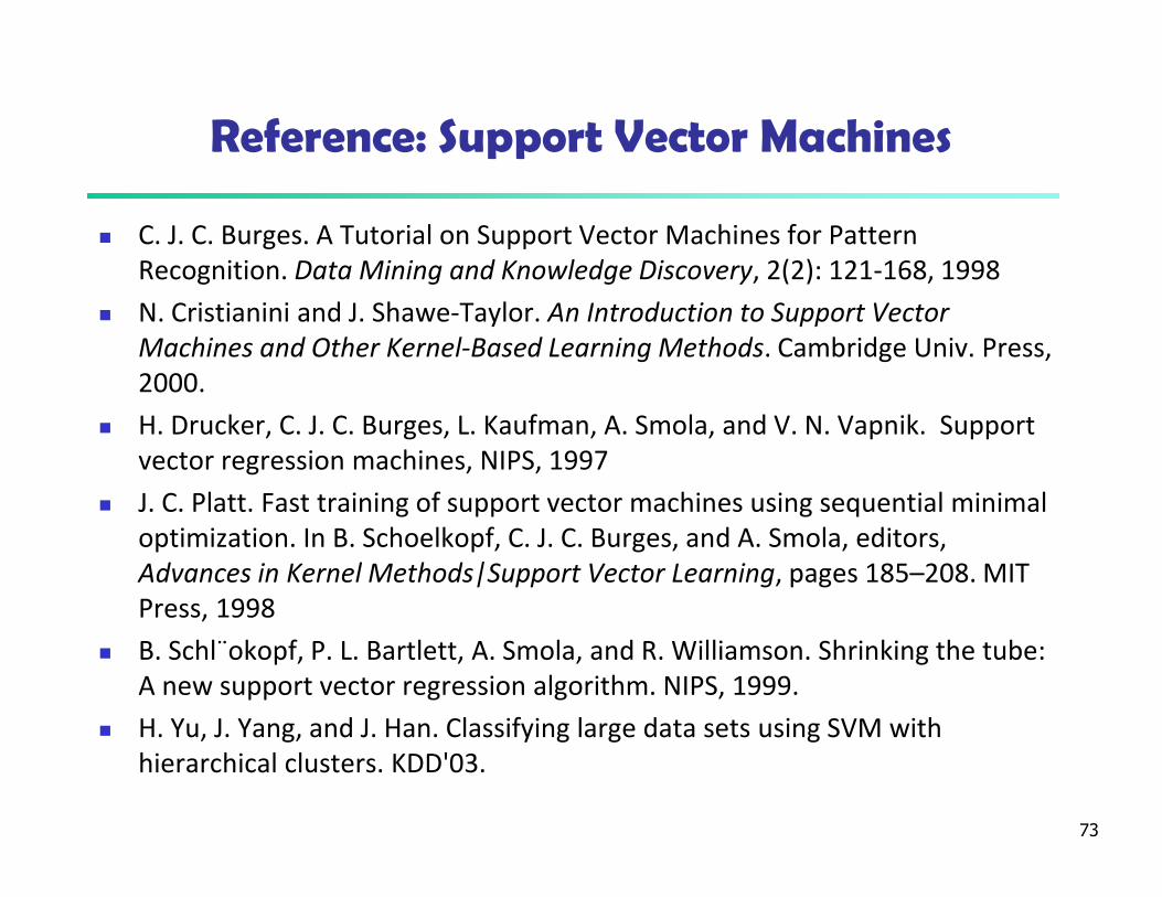
Reference: Support Vector Machines
� C. J. C. Burges. A Tutorial on Support Vector Machines for Pattern
Recognition. Data Mining and Knowledge Discovery, 2(2): 121-168, 1998
� N. Cristianini and J. Shawe-Taylor. An Introduction to Support Vector
Machines and Other Kernel-Based Learning Methods. Cambridge Univ. Press,
2000.
� H. Drucker, C. J. C. Burges, L. Kaufman, A. Smola, and V. N. Vapnik. Support
vector regression machines, NIPS, 1997
� J. C. Platt. Fast training of support vector machines using sequential minimal
optimization. In B. Schoelkopf, C. J. C. Burges, and A. Smola, editors,
Advances in Kernel Methods|Support Vector Learning, pages 185–208. MIT
Press, 1998
� B. Schl¨okopf, P. L. Bartlett, A. Smola, and R. Williamson. Shrinking the tube:
A new support vector regression algorithm. NIPS, 1999.
� H. Yu, J. Yang, and J. Han. Classifying large data sets using SVM with
hierarchical clusters. KDD'03.
73

Reference: Pattern-Based Classification
� H. Cheng, X. Yan, J. Han, and C.-W. Hsu, Discriminative Frequent Pattern Analysis
for Effective Classification, ICDE'07
� H. Cheng, X. Yan, J. Han, and P. S. Yu, Direct Discriminative Pattern Mining for
Effective Classification, ICDE'08
� G. Cong, K.-L. Tan, A. K. H. Tung, and X. Xu. Mining top-k covering rule groups for
gene expression data. SIGMOD'05
� G. Dong and J. Li. Efficient mining of emerging patterns: Discovering trends and
differences. KDD'99
� H. S. Kim, S. Kim, T. Weninger, J. Han, and T. Abdelzaher. NDPMine: Efficiently
mining discriminative numerical features for pattern-based classification.
ECMLPKDD'10
� W. Li, J. Han, and J. Pei, CMAR: Accurate and Efficient Classification Based on
Multiple Class-Association Rules, ICDM'01
� B. Liu, W. Hsu, and Y. Ma. Integrating classification and association rule mining.
KDD'98
� J. Wang and G. Karypis. HARMONY: Efficiently mining the best rules for
classification. SDM'05
74

References: Rule Induction
� P. Clark and T. Niblett. The CN2 induction algorithm. Machine Learning, 3:261–283,
1989.
� W. Cohen. Fast effective rule induction. ICML'95
� S. L. Crawford. Extensions to the CART algorithm. Int. J. Man-Machine Studies, 31:197–
217, Aug. 1989
� J. R. Quinlan and R. M. Cameron-Jones. FOIL: A midterm report. ECML’93
� P. Smyth and R. M. Goodman. An information theoretic approach to rule induction.
IEEE Trans. Knowledge and Data Engineering, 4:301–316, 1992.
� X. Yin and J. Han. CPAR: Classification based on predictive association rules. SDM'03
75
References: K-NN & Case-Based Reasoning
� A. Aamodt and E. Plazas. Case-based reasoning: Foundational
issues, methodological variations, and system approaches. AI
Comm., 7:39–52, 1994.
� T. Cover and P. Hart. Nearest neighbor pattern classification.
IEEE Trans. Information Theory, 13:21–27, 1967
� B. V. Dasarathy. Nearest Neighbor (NN) Norms: NN Pattern
Classication Techniques. IEEE Computer Society Press, 1991
� J. L. Kolodner. Case-Based Reasoning. Morgan Kaufmann, 1993
� A. Veloso, W. Meira, and M. Zaki. Lazy associative classification.
ICDM'06
76

References: Bayesian Method & Statistical Models
� A. J. Dobson. An Introduction to Generalized Linear Models. Chapman & Hall, 1990.
� D. Heckerman, D. Geiger, and D. M. Chickering. Learning Bayesian networks: The
combination of knowledge and statistical data. Machine Learning, 1995.
� G. Cooper and E. Herskovits. A Bayesian method for the induction of probabilistic
networks from data. Machine Learning, 9:309–347, 1992
� A. Darwiche. Bayesian networks. Comm. ACM, 53:80–90, 2010
� A. P. Dempster, N. M. Laird, and D. B. Rubin. Maximum likelihood from incomplete data
via the EM algorithm. J. Royal Statistical Society, Series B, 39:1–38, 1977
� D. Heckerman, D. Geiger, and D. M. Chickering. Learning Bayesian networks: The
combination of knowledge and statistical data. Machine Learning, 20:197–243, 1995
� F. V. Jensen. An Introduction to Bayesian Networks. Springer Verlag, 1996.
� D. Koller and N. Friedman. Probabilistic Graphical Models: Principles and Techniques.
The MIT Press, 2009
� J. Pearl. Probabilistic Reasoning in Intelligent Systems. Morgan Kauffman, 1988
� S. Russell, J. Binder, D. Koller, and K. Kanazawa. Local learning in probabilistic networks
with hidden variables. IJCAI'95
� V. N. Vapnik. Statistical Learning Theory. John Wiley & Sons, 1998.
77

Refs: Semi-Supervised & Multi-Class Learning
� O. Chapelle, B. Schoelkopf, and A. Zien. Semi-supervised
Learning. MIT Press, 2006
� T. G. Dietterich and G. Bakiri. Solving multiclass learning
problems via error-correcting output codes. J. Articial
Intelligence Research, 2:263–286, 1995
� W. Dai, Q. Yang, G. Xue, and Y. Yu. Boosting for transfer
learning. ICML’07
� S. J. Pan and Q. Yang. A survey on transfer learning. IEEE Trans.
on Knowledge and Data Engineering, 22:1345–1359, 2010
� B. Settles. Active learning literature survey. In Computer
Sciences Technical Report 1648, Univ. Wisconsin-Madison, 2010
� X. Zhu. Semi-supervised learning literature survey. CS Tech. Rep.
1530, Univ. Wisconsin-Madison, 200578
Refs: Genetic Algorithms & Rough/Fuzzy Sets
� D. Goldberg. Genetic Algorithms in Search, Optimization, and Machine
Learning. Addison-Wesley, 1989
� S. A. Harp, T. Samad, and A. Guha. Designing application-specific neural
networks using the genetic algorithm. NIPS, 1990
� Z. Michalewicz. Genetic Algorithms + Data Structures = Evolution Programs.
Springer Verlag, 1992.
� M. Mitchell. An Introduction to Genetic Algorithms. MIT Press, 1996
� Z. Pawlak. Rough Sets, Theoretical Aspects of Reasoning about Data. Kluwer
Academic, 1991
� S. Pal and A. Skowron, editors, Fuzzy Sets, Rough Sets and Decision Making
Processes. New York, 1998
� R. R. Yager and L. A. Zadeh. Fuzzy Sets, Neural Networks and Soft Computing.
Van Nostrand Reinhold, 1994
79

References: Model Evaluation, Ensemble Methods
� L. Breiman. Bagging predictors. Machine Learning, 24:123–140, 1996.
� L. Breiman. Random forests. Machine Learning, 45:5–32, 2001.
� C. Elkan. The foundations of cost-sensitive learning. IJCAI'01
� B. Efron and R. Tibshirani. An Introduction to the Bootstrap. Chapman & Hall, 1993.
� J. Friedman and E. P. Bogdan. Predictive learning via rule ensembles. Ann. Applied
Statistics, 2:916–954, 2008.
� T.-S. Lim, W.-Y. Loh, and Y.-S. Shih. A comparison of prediction accuracy, complexity,
and training time of thirty-three old and new classification algorithms. Machine
Learning, 2000.
� J. Magidson. The Chaid approach to segmentation modeling: Chi-squared automatic
interaction detection. In R. P. Bagozzi, editor, Advanced Methods of Marketing
Research, Blackwell Business, 1994.
� J. R. Quinlan. Bagging, boosting, and c4.5. AAAI'96.
� G. Seni and J. F. Elder. Ensemble Methods in Data Mining: Improving Accuracy
Through Combining Predictions. Morgan and Claypool, 2010.
� Y. Freund and R. E. Schapire. A decision-theoretic generalization of on-line learning
and an application to boosting. J. Computer and System Sciences, 199780

Surplus Slides
81
82
Issues: Evaluating Classification Methods
� Accuracy
� classifier accuracy: predicting class label
� predictor accuracy: guessing value of predicted attributes
� Speed
� time to construct the model (training time)
� time to use the model (classification/prediction time)
� Robustness: handling noise and missing values
� Scalability: efficiency in disk-resident databases
� Interpretability
� understanding and insight provided by the model
� Other measures, e.g., goodness of rules, such as decision tree size or compactness of classification rules
83
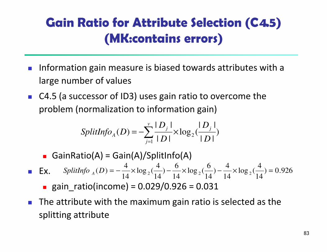
Gain Ratio for Attribute Selection (C4.5) (MK:contains errors)
� Information gain measure is biased towards attributes with a
large number of values
� C4.5 (a successor of ID3) uses gain ratio to overcome the
problem (normalization to information gain)
� GainRatio(A) = Gain(A)/SplitInfo(A)
� Ex.
� gain_ratio(income) = 0.029/0.926 = 0.031
� The attribute with the maximum gain ratio is selected as the
splitting attribute
)||
||(log
||
||)( 2
1 D
D
D
DDSplitInfo
jv
j
j
A ×−= ∑=
926.0)14
4(log
14
4)
14
6(log
14
6)
14
4(log
14
4)( 222 =×−×−×−=DSplitInfo A
84
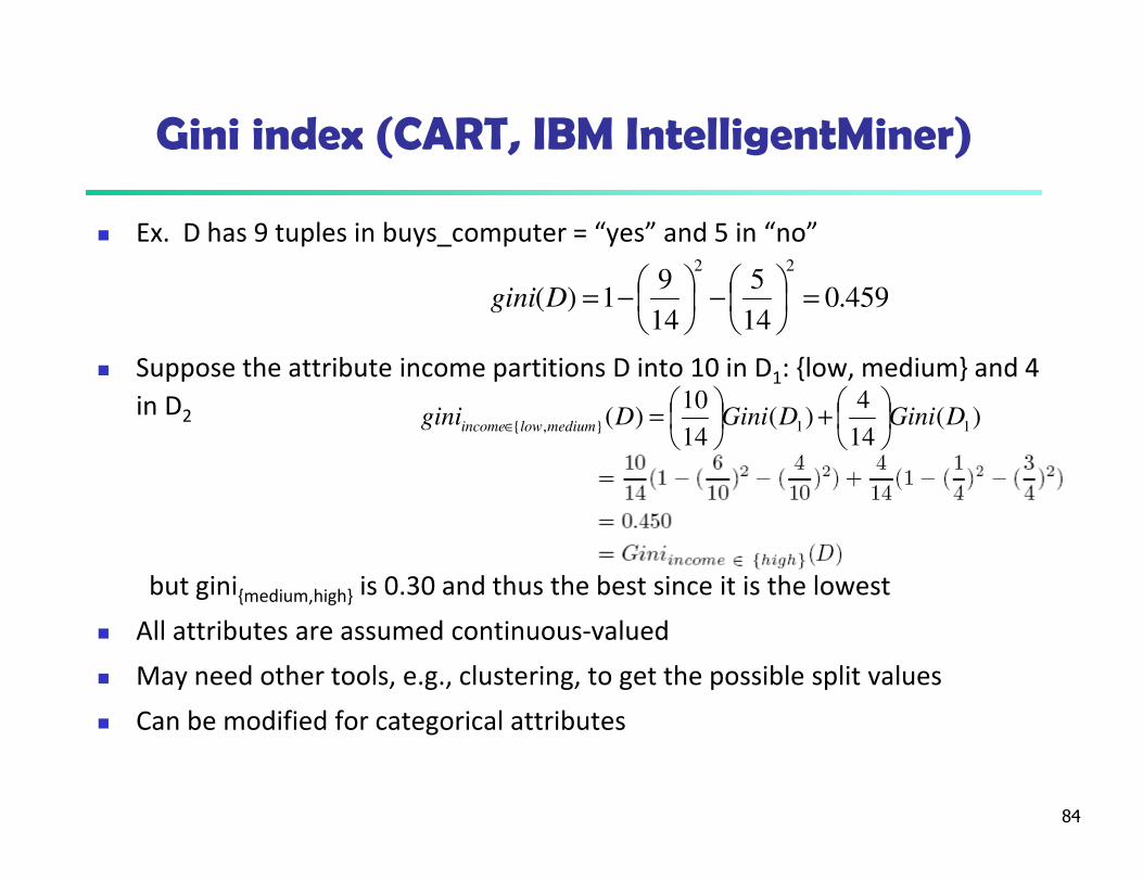
Gini index (CART, IBM IntelligentMiner)
� Ex. D has 9 tuples in buys_computer = “yes” and 5 in “no”
� Suppose the attribute income partitions D into 10 in D1: {low, medium} and 4
in D2
but gini{medium,high} is 0.30 and thus the best since it is the lowest
� All attributes are assumed continuous-valued
� May need other tools, e.g., clustering, to get the possible split values
� Can be modified for categorical attributes
459.014
5
14
91)(
22
=
−
−=Dgini
)(14
4)(
14
10)( 11},{ DGiniDGiniDgini mediumlowincome
+
=∈
85
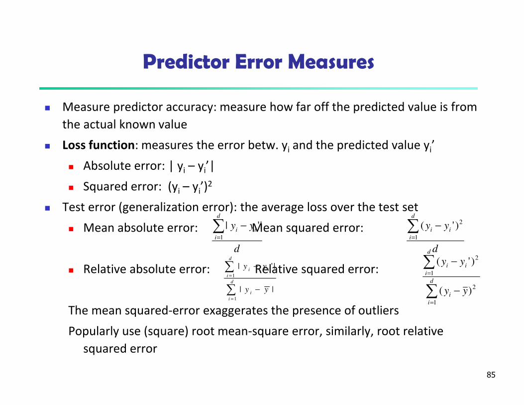
Predictor Error Measures
� Measure predictor accuracy: measure how far off the predicted value is from
the actual known value
� Loss function: measures the error betw. yi and the predicted value yi’
� Absolute error: | yi – yi’|
� Squared error: (yi – yi’)2
� Test error (generalization error): the average loss over the test set
� Mean absolute error: Mean squared error:
� Relative absolute error: Relative squared error:
The mean squared-error exaggerates the presence of outliers
Popularly use (square) root mean-square error, similarly, root relative
squared error
d
yyd
i
ii∑=
−1
|'|
d
yyd
i
ii∑=
−1
2)'(
∑
∑
=
=
−
−
d
i
i
d
i
ii
yy
yy
1
1
||
|'|
∑
∑
=
=
−
−
d
i
i
d
i
ii
yy
yy
1
2
1
2
)(
)'(

86
Scalable Decision Tree Induction Methods
� SLIQ (EDBT’96 — Mehta et al.)
� Builds an index for each attribute and only class list and the
current attribute list reside in memory
� SPRINT (VLDB’96 — J. Shafer et al.)
� Constructs an attribute list data structure
� PUBLIC (VLDB’98 — Rastogi & Shim)
� Integrates tree splitting and tree pruning: stop growing the
tree earlier
� RainForest (VLDB’98 — Gehrke, Ramakrishnan & Ganti)
� Builds an AVC-list (attribute, value, class label)
� BOAT (PODS’99 — Gehrke, Ganti, Ramakrishnan & Loh)
� Uses bootstrapping to create several small samples

87
Data Cube-Based Decision-Tree Induction
� Integration of generalization with decision-tree induction
(Kamber et al.’97)
� Classification at primitive concept levels
� E.g., precise temperature, humidity, outlook, etc.
� Low-level concepts, scattered classes, bushy classification-
trees
� Semantic interpretation problems
� Cube-based multi-level classification
� Relevance analysis at multi-levels
� Information-gain analysis with dimension + level
Recommended