Download pdf - Data Mining-Project Report Gene Classification using Neural Network- Apil Tamang

Data Mining Fall 2013

Project Report

Apil Tamang

Gene Classification using Neural Networks

Introduction

Problem:

Genes play a fundamental role in any living organism’s life. The processes of life are controlled by

proteins that are produced within an organism’s cells. Functions such as muscle movement, food

digestion, production of energy, waste removal, producing antibodies to fight infection etc. are all

controlled by the production of proteins within an organism. Fundamental processes such as breathing,

heartbeats, growth and regeneration etc. are all dependent on the production of the right kind of

proteins at the right places and moments of time. In other words, life is sustained by proteins: many

different kinds of them!

The synthesis of proteins is controlled by genes. A gene is a certain length of DNA that is found within

the chromosomes within the nucleus of an organism. It consists of a sequence of DNA base pairs:

specifically, four different kinds. They are (A)denine, (T)hymine, (G)uanine, and (C)ytosine. Only certain

specific regions within in the DNA serve as protein synthesizing elements. Each gene results in the

production of one and only one kind of protein. The genes for the entire set of proteins available to an

organism are found within the chromosomes. Hence, the DNA is also called the code for life.

The entire DNA sequence contains many different kinds of sequences in addition to genes. There are

regions that serve as binding sites for other processes, regions that signal the beginning and end of the

gene regions, and regions that serve absolutely no purpose (to current knowledge), to name a few.

Much of the entire DNA sequence is not quite understood about. For e.g. it is estimated that only 2% of

the entire DNA sequence of human serve as genes. Researchers do not know for sure what the purpose

of the rest of the DNA is.

In this project, we examine the DNA of lower-class organisms where the entire DNA sequence can be

divided into two main categories: the coding (gene), and the non-coding (non-gene) regions. The files

containing sequences for all the proteins known to two organisms: E. Coli (Strain MG1665) and

A.Baccillus were downloaded from the NCBI genome repository. The work is based on the hypothesis

that the coding regions have a certain pattern in their gene statistics which makes it possible to identify

them from the innumerable sequence combinations that can be constructed from the DNA sequence.

We mentioned previously that most of the DNA itself consists of non-coding regions. Hence, the attempt

is to look at a sample of DNA sequence and be able to tell if it is a coding sequence or a non-coding

sequence, i.e. a gene or a non-gene region, respectively. We go a step further and see if there is any

specific pattern that can be inferred from the genes of two different organisms such that this

information can be used to correctly identify which organism the given sample is from.

Neural Networks:

Neural Networks are computer algorithms that can be used to solve many classes of artificial

intelligence problems. These problems can range from optimization to classification. The major

constituent elements of a neural network are neurons, connections, weights and transformation

functions. The neurons themselves are modeled after their biological counterparts that serve a central

role of survival in higher-class organisms. Neurons are specialized cells capable of receiving electrical

signals and transmitting them after some processing. They are also capable of forming interconnections

within the organism and control the movement of virtually every muscle in the organism. Neurons

constitute the central nervous system (i.e. brain and spinal cord) by forming a massive and very complex

web of connections between themselves. Thus, neurons are also the seat of intelligence and memory in

higher-class organisms.

The neurons in the neural network algorithm have very similar features. They are able to take in an

input and form connections with the neighboring neurons. Weights are the signals that neurons pass

amongst each other during a computation process. Each neuron is capable of processing the input via a

mathematical function that can be specified by a user. In a typical network, neurons communicate by

passing weights around. The output of a network is the overall collective processing performed by each

neuron as it communicates with other neurons in the network. In this way, neural networks often

provide a black-box like problem solving tool for the end user.

There are many different kinds of neural networks available in the field. These networks differ from each

other by the kind of function they use for processing the input, the way they are interconnected in the

network, and the way information is passed around in the system before an end result is displayed. In

this class project, we have used a fully interconnected Multilayer Perceptron network with the standard

forward-feed, back-propagation learning algorithm. This setup is optimal for classification and is widely

used for this class of problems.

Methodology

Data preprocessing:

The building block of proteins is the amino acid. An amino acid consists of a set of three DNA base pair

sequence. This set of three DNA base pair is also referred to as a codon. Given that there are 4 kinds of

DNA base pairs, there are 64 possible kinds of codons that can be formed by this set of sequence. There

are 20 different amino acids identified by scientists and researchers. Hence, there is a many-to-one

mapping from codons to amino acids.

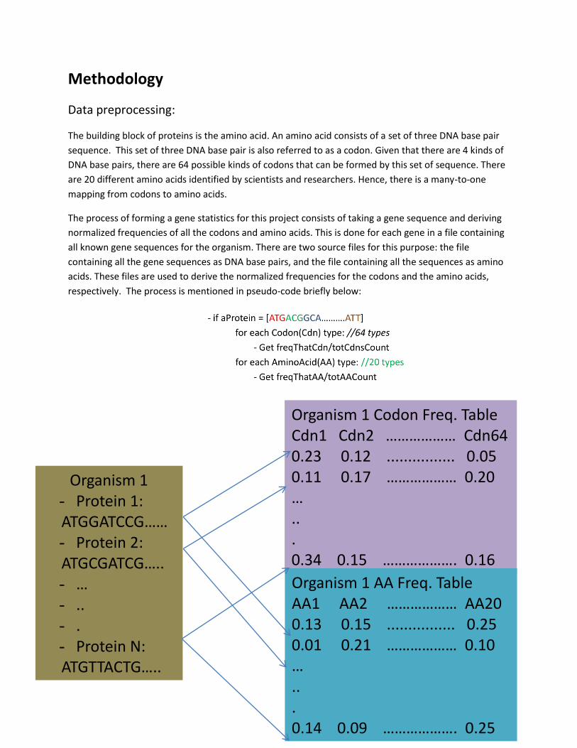
The process of forming a gene statistics for this project consists of taking a gene sequence and deriving

normalized frequencies of all the codons and amino acids. This is done for each gene in a file containing

all known gene sequences for the organism. There are two source files for this purpose: the file

containing all the gene sequences as DNA base pairs, and the file containing all the sequences as amino

acids. These files are used to derive the normalized frequencies for the codons and the amino acids,

respectively. The process is mentioned in pseudo-code briefly below:

Organism 1

- Protein 1: ATGGATCCG……

- Protein 2: ATGCGATCG…..

- … - .. - . - Protein N:

ATGTTACTG…..

Organism 1 Codon Freq. Table

Cdn1 Cdn2 ……………… Cdn64

0.23 0.12 ................ 0.05

0.11 0.17 ……………… 0.20

…

..

. 0.34 0.15 ………………. 0.16

Organism 1 AA Freq. Table

AA1 AA2 ……………… AA20

0.13 0.15 ................ 0.25

0.01 0.21 ……………… 0.10

…

..

. 0.14 0.09 ………………. 0.25

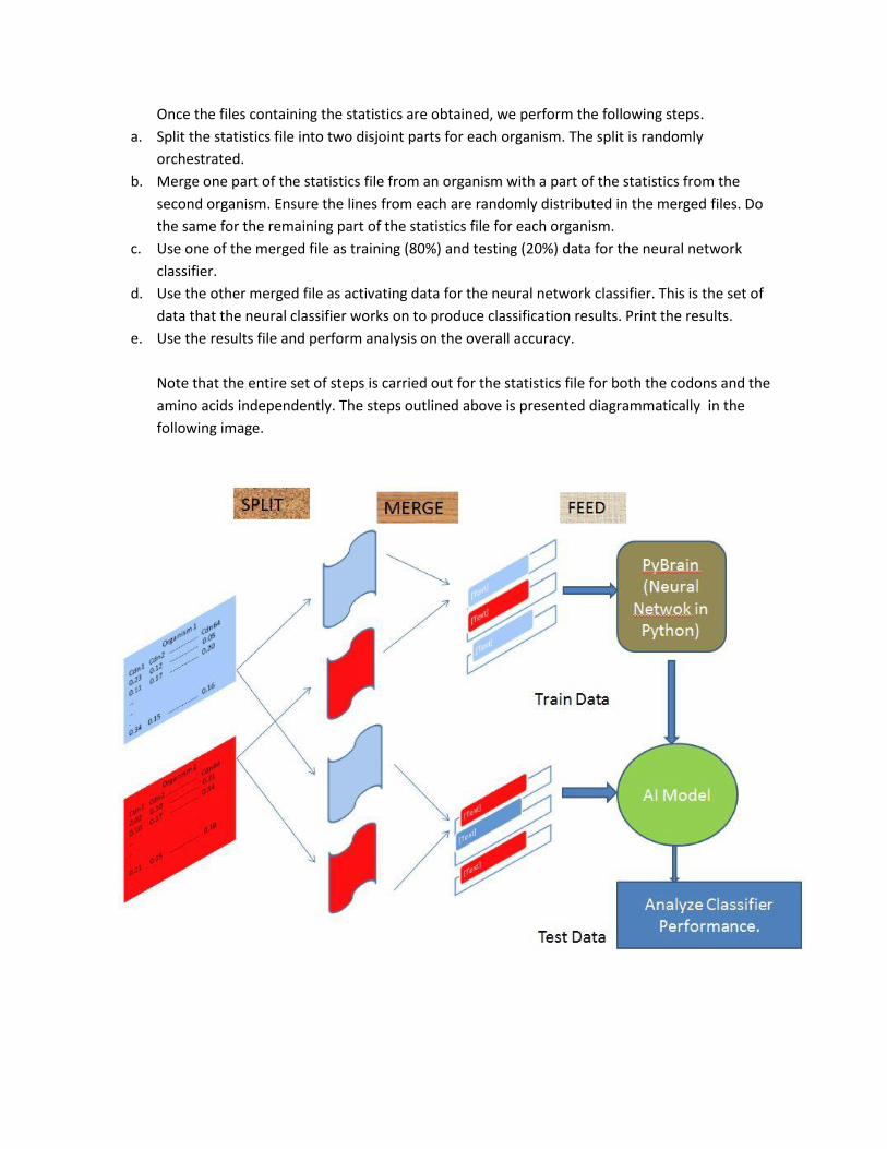
Once the files containing the statistics are obtained, we perform the following steps.

a. Split the statistics file into two disjoint parts for each organism. The split is randomly

orchestrated.

b. Merge one part of the statistics file from an organism with a part of the statistics from the

second organism. Ensure the lines from each are randomly distributed in the merged files. Do

the same for the remaining part of the statistics file for each organism.

c. Use one of the merged file as training (80%) and testing (20%) data for the neural network

classifier.

d. Use the other merged file as activating data for the neural network classifier. This is the set of

data that the neural classifier works on to produce classification results. Print the results.

e. Use the results file and perform analysis on the overall accuracy.

Note that the entire set of steps is carried out for the statistics file for both the codons and the

amino acids independently. The steps outlined above is presented diagrammatically in the

following image.

Classifier Setup:

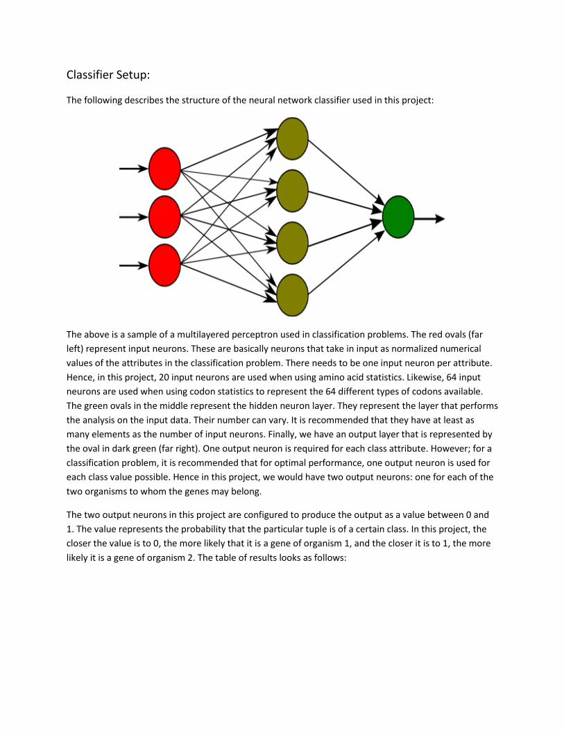
The following describes the structure of the neural network classifier used in this project:

The above is a sample of a multilayered perceptron used in classification problems. The red ovals (far

left) represent input neurons. These are basically neurons that take in input as normalized numerical

values of the attributes in the classification problem. There needs to be one input neuron per attribute.

Hence, in this project, 20 input neurons are used when using amino acid statistics. Likewise, 64 input

neurons are used when using codon statistics to represent the 64 different types of codons available.

The green ovals in the middle represent the hidden neuron layer. They represent the layer that performs

the analysis on the input data. Their number can vary. It is recommended that they have at least as

many elements as the number of input neurons. Finally, we have an output layer that is represented by

the oval in dark green (far right). One output neuron is required for each class attribute. However; for a

classification problem, it is recommended that for optimal performance, one output neuron is used for

each class value possible. Hence in this project, we would have two output neurons: one for each of the

two organisms to whom the genes may belong.

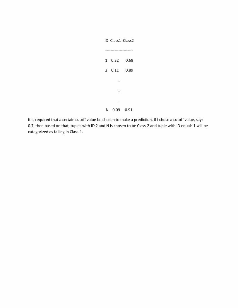
The two output neurons in this project are configured to produce the output as a value between 0 and

1. The value represents the probability that the particular tuple is of a certain class. In this project, the

closer the value is to 0, the more likely that it is a gene of organism 1, and the closer it is to 1, the more

likely it is a gene of organism 2. The table of results looks as follows:

ID Class1 Class2

---------------------

1 0.32 0.68

2 0.11 0.89

…

..

.

N 0.09 0.91

It is required that a certain cutoff value be chosen to make a prediction. If I chose a cutoff value, say:

0.7, then based on that, tuples with ID 2 and N is chosen to be Class-2 and tuple with ID equals 1 will be

categorized as falling in Class-1.

Results

Problem 1:

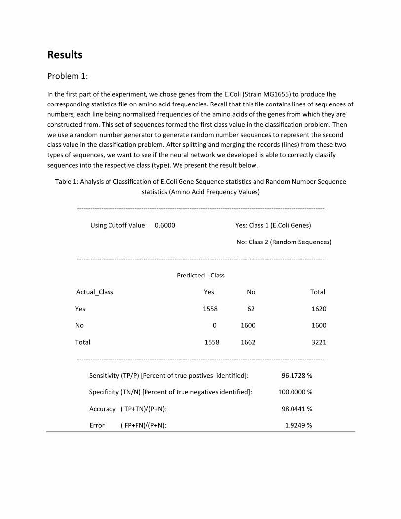
In the first part of the experiment, we chose genes from the E.Coli (Strain MG1655) to produce the

corresponding statistics file on amino acid frequencies. Recall that this file contains lines of sequences of

numbers, each line being normalized frequencies of the amino acids of the genes from which they are

constructed from. This set of sequences formed the first class value in the classification problem. Then

we use a random number generator to generate random number sequences to represent the second

class value in the classification problem. After splitting and merging the records (lines) from these two

types of sequences, we want to see if the neural network we developed is able to correctly classify

sequences into the respective class (type). We present the result below.

Table 1: Analysis of Classification of E.Coli Gene Sequence statistics and Random Number Sequence

statistics (Amino Acid Frequency Values)

----------------------------------------------------------------------------------------------------------------

Using Cutoff Value: 0.6000 Yes: Class 1 (E.Coli Genes)

No: Class 2 (Random Sequences)

----------------------------------------------------------------------------------------------------------------

Predicted - Class

Actual_Class Yes No Total

Yes 1558 62 1620

No 0 1600 1600

Total 1558 1662 3221

----------------------------------------------------------------------------------------------------------------

Sensitivity (TP/P) [Percent of true postives identified]: 96.1728 %

Specificity (TN/N) [Percent of true negatives identified]: 100.0000 %

Accuracy ( TP+TN)/(P+N): 98.0441 %

Error ( FP+FN)/(P+N): 1.9249 %

Additional setup parameters:

For this problem, the momentum for learning was set to 0.5 and the weightdecay was set to 0.001. 20

neurons were used in the hidden layer (equal to the number of input neurons). The total mean-square

error at the end of 20 cycles for training was 0.0484.

Discussion:

We can see that our neural network is able to classify the two sequences with very high precision. By

setting the cutoff value at 0.6, we were able to correctly identify 1558 out of 1620 sequences that were

derived from the genes of the E.Coli. That represents 96.2% of the total gene used for testing the neural

classifier. In addition, no random sequences were classified as a sequence type derived from E.Coli

genes. That represents a 100% accuracy of identifying random sequences from gene sequences. We do

not perform the same analysis using statistics for the codon tables for this problem set. We realize that

we already achieved very high accuracy. Next, we present results obtained for using the classifier on

genes sequences derived from two different organisms: E. Coli, and A. Baci, where both are bacterial

species.

Problem 2:

In the next experiment, we use gene sequences from two different organisms. The results of the first

experiment suggest that the random number sequences must be very easily identifiable from the

sequences resulting from the analysis of actual gene statistics. Hence, we prepare statistics from two

real organisms to test and see if there are any discernible patterns in their genes. We expect the

classifier to yield slightly poorer results than the first experiment did. This is because we expect that

although the genes could be derived from two different organisms, they would still have a large set of

similarities resulting from the fact that both these sets are genes that actually support biological life. We

present the results on the following pages.

Table 2: Analysis of Classification of A. Baci and E. Coli Gene Sequence statistics (Amino Acid Values)

----------------------------------------------------------------------------------------------------------------

Using Cutoff Value: 0.5000 Yes: Class 1 (A. Baci Genes)

No: Class 2 (E. Coli Genes)

----------------------------------------------------------------------------------------------------------------

Predicted - Class


Yes 822 411 1233

No 128 1493 1621

Total 950 1904 2855

----------------------------------------------------------------------------------------------------------------




Error ( FP+FN)/(P+N): 18.88 %

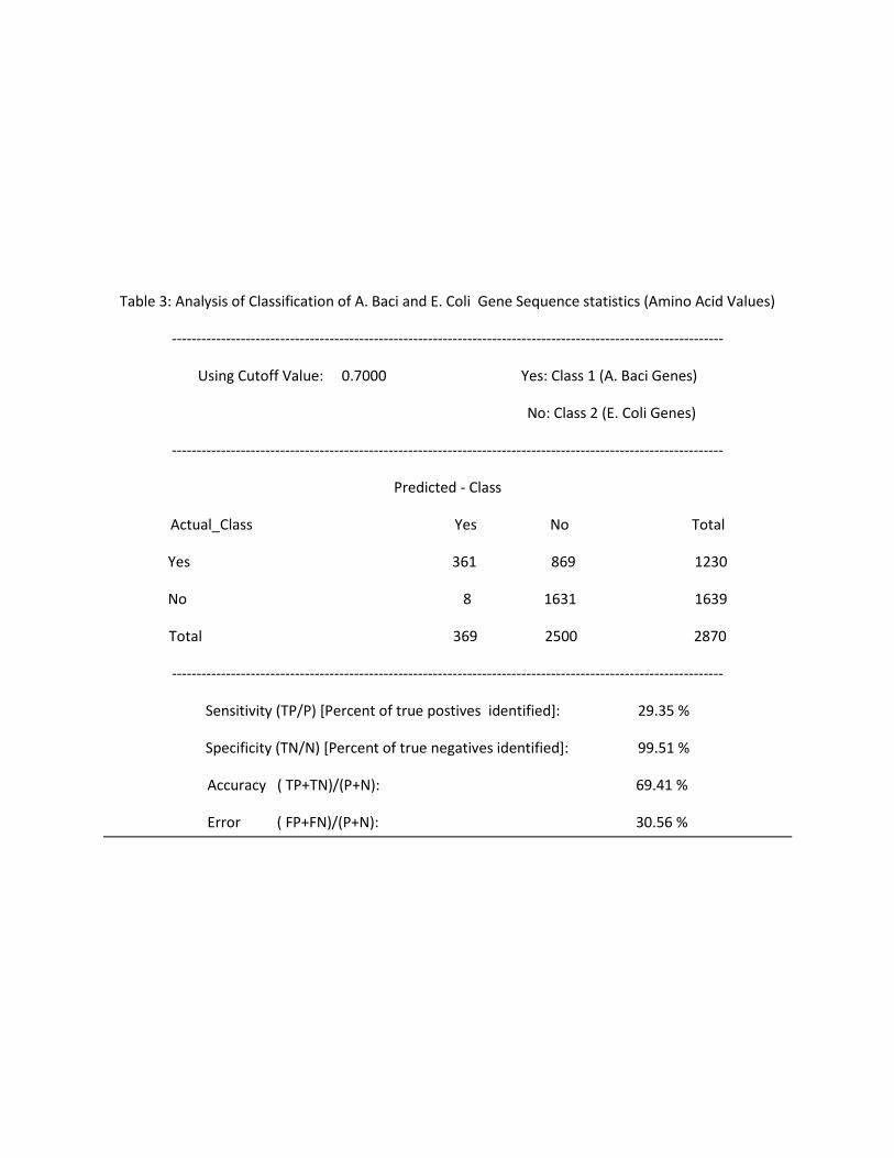
Table 3: Analysis of Classification of A. Baci and E. Coli Gene Sequence statistics (Amino Acid Values)

----------------------------------------------------------------------------------------------------------------



----------------------------------------------------------------------------------------------------------------

Predicted - Class


Yes 361 869 1230

No 8 1631 1639

Total 369 2500 2870

----------------------------------------------------------------------------------------------------------------




Error ( FP+FN)/(P+N): 30.56 %

Table 4: Analysis of Classification of A. Baci and E. Coli Gene Sequence statistics (Codon Values)

----------------------------------------------------------------------------------------------------------------



----------------------------------------------------------------------------------------------------------------

Predicted - Class


Yes 1181 68 1249

No 10 1609 1619

Total 1191 1677 2869

----------------------------------------------------------------------------------------------------------------




Error ( FP+FN)/(P+N): 2.72 %

Table 5: Analysis of Classification of A. Baci and E. Coli Gene Sequence statistics (Codon Values)

----------------------------------------------------------------------------------------------------------------



----------------------------------------------------------------------------------------------------------------

Predicted - Class


Yes 1043 181 1224

No 2 1650 1652

Total 1045 1831 2877

----------------------------------------------------------------------------------------------------------------




Error ( FP+FN)/(P+N): 6.36 %

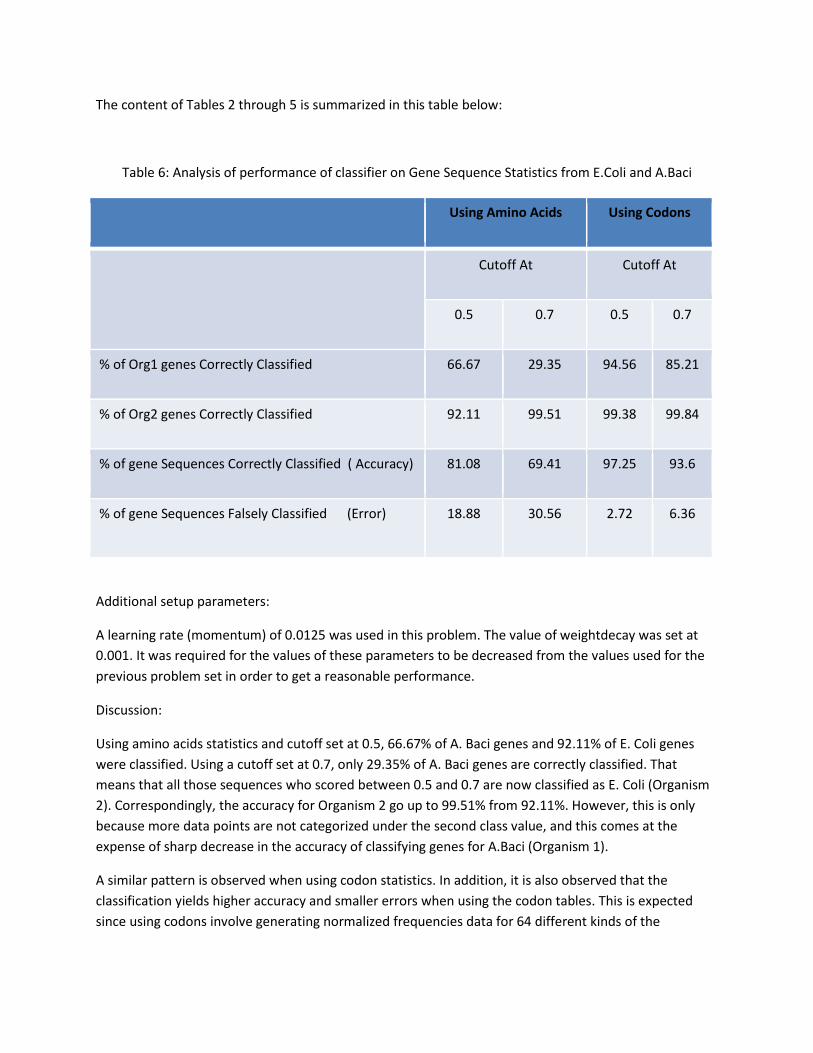
The content of Tables 2 through 5 is summarized in this table below:

Table 6: Analysis of performance of classifier on Gene Sequence Statistics from E.Coli and A.Baci

Using Amino Acids Using Codons

Cutoff At Cutoff At

0.5 0.7 0.5 0.7

% of Org1 genes Correctly Classified 66.67 29.35 94.56 85.21

% of Org2 genes Correctly Classified 92.11 99.51 99.38 99.84

% of gene Sequences Correctly Classified ( Accuracy) 81.08 69.41 97.25 93.6

% of gene Sequences Falsely Classified (Error) 18.88 30.56 2.72 6.36

Additional setup parameters:

A learning rate (momentum) of 0.0125 was used in this problem. The value of weightdecay was set at

0.001. It was required for the values of these parameters to be decreased from the values used for the

previous problem set in order to get a reasonable performance.

Discussion:

Using amino acids statistics and cutoff set at 0.5, 66.67% of A. Baci genes and 92.11% of E. Coli genes

were classified. Using a cutoff set at 0.7, only 29.35% of A. Baci genes are correctly classified. That

means that all those sequences who scored between 0.5 and 0.7 are now classified as E. Coli (Organism

2). Correspondingly, the accuracy for Organism 2 go up to 99.51% from 92.11%. However, this is only

because more data points are not categorized under the second class value, and this comes at the

expense of sharp decrease in the accuracy of classifying genes for A.Baci (Organism 1).

A similar pattern is observed when using codon statistics. In addition, it is also observed that the

classification yields higher accuracy and smaller errors when using the codon tables. This is expected

since using codons involve generating normalized frequencies data for 64 different kinds of the

respective codons. Using amino acids involve data for 20 different kinds of amino acids. Hence, there is

more information to help the classifier perform the classification using the codon values.

Summary and Future Work:

In this project, the neural network algorithm was used to perform classification of gene sequences

based on the statistics of the frequencies of their building blocks: amino acids, and codons. The

experiment was conducted independently for both these elementary constituents of the genes. The first

experiment involved classification of the gene sequences with sequences generated by random

numbers. The neural network classifier was easily able to sort them out with high precision. The second

experiment involved sequence classification of genes from two different organisms. With some changes

in the learning parameters and the weightdecay values, a reasonable degree of precision was achieved

again. It was observed as we expected that using codon statistics results in higher precision than using

amino acid statistics. However, this comes at added expense in computation since the former uses 64

input neurons versus 20 input neurons used by the latter.

As future work, this work could be extended to perform classification of additional types of genetic

material. In lower class organisms, their genome contains primarily two kinds of regions: the coding

(gene) and the non-coding (non-gene) regions. Higher-class organisms contain far more variety of

regions within their genome, for e.g. regions for binding other chemical processes, regions for splicing,

encoding and passive regions within a single gene sequence, and so on and so forth. Each region is

characterized by a specific statistical pattern of the constituent amino acid and corresponding codons.

Hence, the method developed in this project could be used to perform the same kind of statistical

classification of these many kinds of regions within a higher-class organism’s genome.

References:

[1] Harold, F. M. (2001). The way of the cell: Molecules, organisms, and the orders of life. (1st ed.).

Oxford University Press.

[2] Michal Q., Z. (2002). Computational prediction of eukaryotic protein-coding genes. Nature , 3, 698-

709. Retrieved from www.cs.odu.edu/~pothen/Courses/CS791/zhang.pdf

[3] Johansen, O. (2008). Gene splice site prediction using artifical neural networks. (Master's thesis).

[4] Turban, E. (2011). Neural networks and data mining. In R. Sharda & D. Delen (Eds.), Business

Intelligence: A Managerial Approach (2nd ed.). Retrieved from

http://www70.homepage.villanova.edu/matthew.liberatore/Mgt2206/turban_online_ch06.pdf

[5] Pybrain: The machine learning library. (11, 12 2009). Retrieved from

http://pybrain.org/docs/index.html

http://www70.homepage.villanova.edu/matthew.liberatore/Mgt2206/turban_online_ch06.pdf

http://pybrain.org/docs/index.html