CS623: Introduction to Computing with Neural Nets
Pushpak BhattacharyyaComputer Science and Engineering
DepartmentIIT Bombay

The human brain
Seat of consciousness and cognition
Perhaps the most complex information processing machine in nature
Historically, considered as a monolithic information processing machine

Beginner’s Brain Map
Forebrain (Cerebral Cortex): Language, maths, sensation, movement, cognition, emotion
Cerebellum: Motor Control
Midbrain: Information Routing; involuntary controls
Hindbrain: Control of breathing, heartbeat, blood circulation
Spinal cord: Reflexes, information highways between body & brain

Brain : a computational machine?
Information processing: brains vs computers
brains better at perception / cognition slower at numerical calculations parallel and distributed Processing associative memory

Brain : a computational machine? (contd.)
• Evolutionarily, brain has developed algorithms most suitable for survival
• Algorithms unknown: the search is on• Brain astonishing in the amount of
information it processes– Typical computers: 109 operations/sec– Housefly brain: 1011 operations/sec
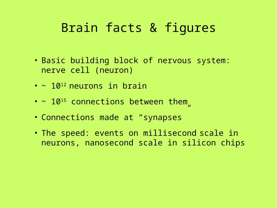
Brain facts & figures
• Basic building block of nervous system: nerve cell (neuron)
• ~ 1012 neurons in brain
• ~ 1015 connections between them
• Connections made at “synapses”
• The speed: events on millisecond scale in neurons, nanosecond scale in silicon chips

Neuron - “classical”
• Dendrites– Receiving stations of neurons– Don't generate action potentials
• Cell body– Site at which information
received is integrated
• Axon– Generate and relay action
potential– Terminal
• Relays information to
next neuron in the pathwayhttp://www.educarer.com/images/brain-nerve-axon.jpg

Computation in Biological Neuron
• Incoming signals from synapses are summed up at the soma
• , the biological “inner product”• On crossing a threshold, the cell “fires” generating
an action potential in the axon hillock region
Synaptic inputs: Artist’s conception

The biological neuron
Pyramidal neuron, from the amygdala (Rupshi et al. 2005)
A CA1 pyramidal neuron (Mel et al. 2004)

A perspective of AI Artificial Intelligence - Knowledge based computing Disciplines which form the core of AI - inner circle Fields which draw from these disciplines - outer circle.
Planning
CV
NLP
ExpertSystems
Robotics
Search, RSN,LRN

Symbolic AI
Connectionist AI is contrasted with Symbolic AISymbolic AI - Physical Symbol System Hypothesis
Every intelligent system can be constructed by storing and processing symbols and nothing more is necessary.
Symbolic AI has a bearing on models of computation such as
Turing Machine Von Neumann Machine Lambda calculus
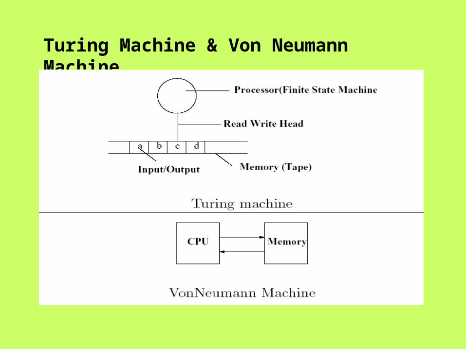
Turing Machine & Von Neumann Machine
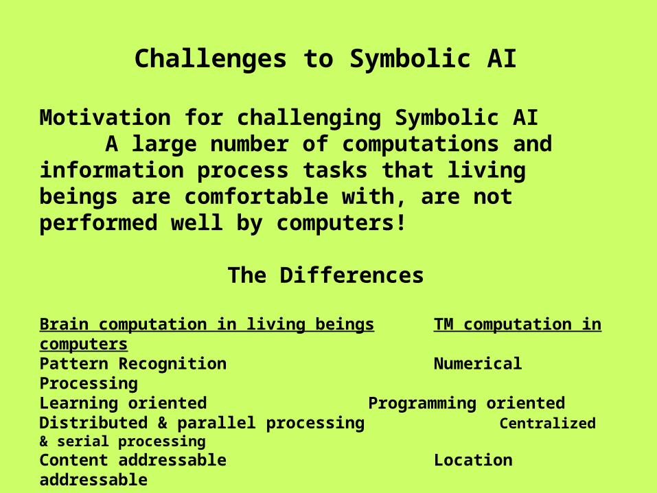
Challenges to Symbolic AI
Motivation for challenging Symbolic AIA large number of computations and
information process tasks that living beings are comfortable with, are not performed well by computers!
The Differences
Brain computation in living beings TM computation in computersPattern Recognition Numerical ProcessingLearning oriented Programming orientedDistributed & parallel processing Centralized & serial processingContent addressable Location addressable

Perceptron

The Perceptron Model
A perceptron is a computing element with input lines having associated weights and the cell having a threshold value. The perceptron model is motivated by the biological neuron.
Output = y
wnWn-1
w1
Xn-1
x1
Threshold = θ
θ
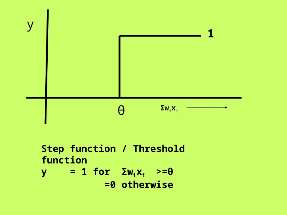
1y
Step function / Threshold functiony = 1 for Σwixi >=θ =0 otherwise
Σwixi

Features of Perceptron
• Input output behavior is discontinuous and the derivative does not exist at Σwixi = θ
• Σwixi - θ is the net input denoted as net
• Referred to as a linear threshold element - linearity because of x appearing with power 1
• y= f(net): Relation between y and net is non-linear
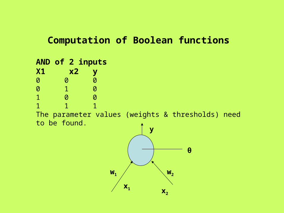
Computation of Boolean functions
AND of 2 inputsX1 x2 y0 0 00 1 01 0 01 1 1The parameter values (weights & thresholds) need to be found.
y
w1 w2
x1 x2
θ

Computing parameter values
w1 * 0 + w2 * 0 <= θ θ >= 0; since y=0
w1 * 0 + w2 * 1 <= θ w2 <= θ; since y=0
w1 * 1 + w2 * 0 <= θ w1 <= θ; since y=0
w1 * 1 + w2 *1 > θ w1 + w2 > θ; since y=1w1 = w2 = = 0.5
satisfy these inequalities and find parameters to be used for computing AND function.
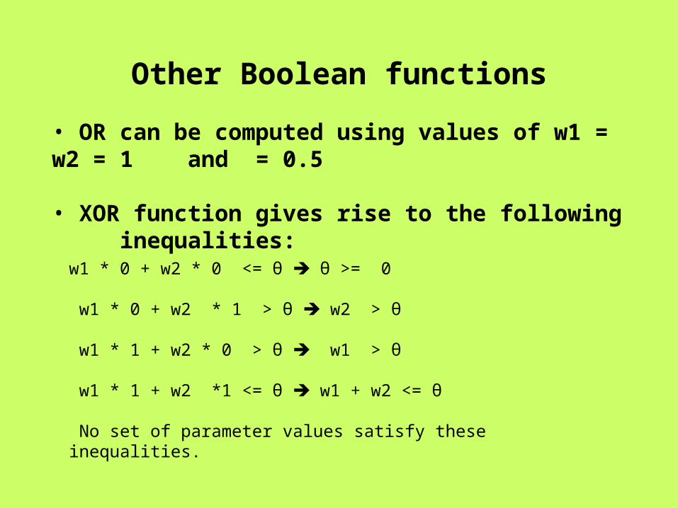
Other Boolean functions
• OR can be computed using values of w1 = w2 = 1 and = 0.5
• XOR function gives rise to the following inequalities:
w1 * 0 + w2 * 0 <= θ θ >= 0
w1 * 0 + w2 * 1 > θ w2 > θ
w1 * 1 + w2 * 0 > θ w1 > θ
w1 * 1 + w2 *1 <= θ w1 + w2 <= θ
No set of parameter values satisfy these inequalities.
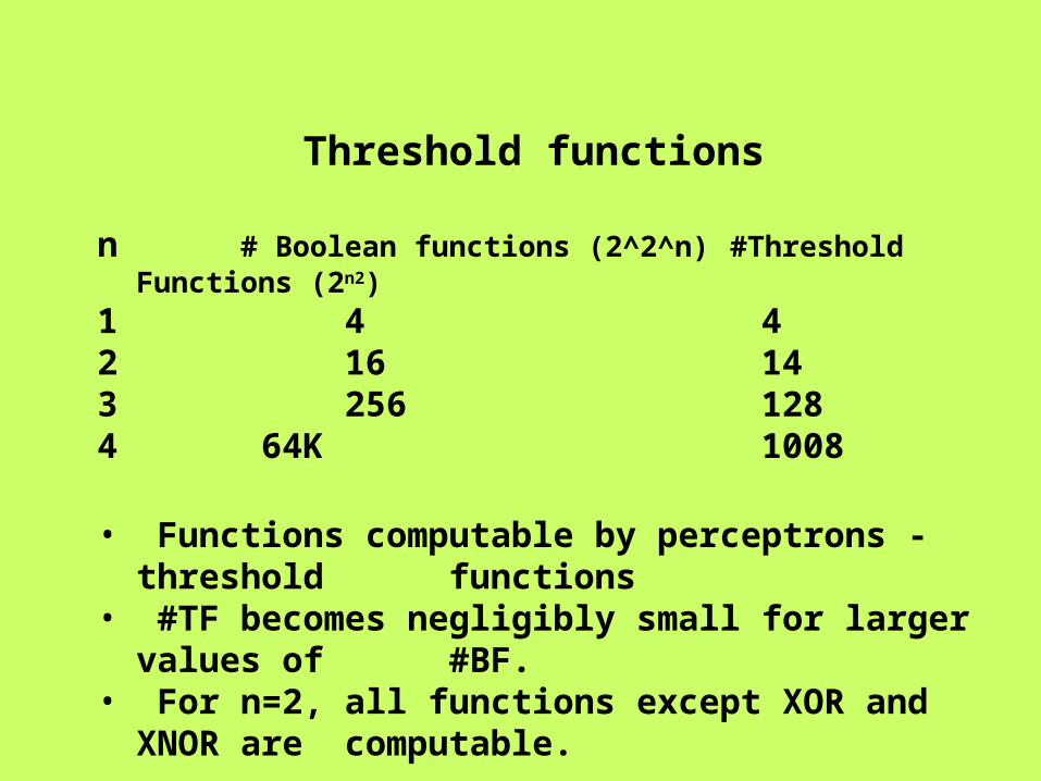
Threshold functions
n # Boolean functions (2^2^n) #Threshold Functions (2n2)
1 4 42 16 143 256 1284 64K 1008
• Functions computable by perceptrons - threshold functions
• #TF becomes negligibly small for larger values of #BF.
• For n=2, all functions except XOR and XNOR are computable.

Concept of Hyper-planes
• ∑ wixi = θ defines a linear surface in the (W,θ) space, where W=<w1,w2,w3,…,wn> is an n-dimensional vector.
• A point in this (W,θ) space
defines a perceptron.
y
x1
. . .
θ
w1 w2 w3 wn
x2 x3 xn

Perceptron Property
• Two perceptrons may have different parameters but same functional values.
• Example of the simplest perceptron w.x>0 gives y=1
w.x≤0 gives y=0 Depending on different values of w and θ, four different functions are
possible
θ
y
x1
w1

Simple perceptron contd.
10101
11000
f4f3f2f1x
θ≥0w≤0
θ≥0w>0
θ<0w≤0
θ<0W<0
0-function Identity Function Complement Function
True-Function

Counting the number of functions for the simplest perceptron
• For the simplest perceptron, the equation is w.x=θ.
Substituting x=0 and x=1,
we get θ=0 and w=θ.
These two lines intersect to
form four regions, which
correspond to the four functions.
θ=0
w=θ
R1
R2R3
R4

Fundamental Observation
• The number of TFs computable by a perceptron is equal to the number of regions produced by 2n hyper-planes,obtained by plugging in the values <x1,x2,x3,…,xn> in the equation
∑i=1nwixi= θ
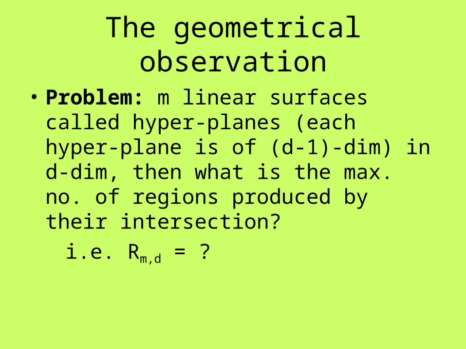
The geometrical observation
• Problem: m linear surfaces called hyper-planes (each hyper-plane is of (d-1)-dim) in d-dim, then what is the max. no. of regions produced by their intersection?
i.e. Rm,d = ?

Perceptron Training Algorithm (PTA)
Preprocessing:
1. The computation law is modified to
y = 1 if ∑wixi > θ
y = o if ∑wixi < θ
. . .
θ, ≤
w1 w2 wn
x1 x2 x3 xn
. . .
θ, <
w1 w2 w3wn
x1 x2 x3 xn
w3

PTA – preprocessing cont…
2. Absorb θ as a weight
3. Negate all the zero-class examples
. . .
θ
w1 w2 w3 wn
x2 x3 xnx1
w0=θ
x0= -1
. . .
θ
w1 w2 w
3
wn
x2 x3 xnx1

Example to demonstrate preprocessing
• OR perceptron1-class <1,1> , <1,0> , <0,1>0-class <0,0>
Augmented x vectors:-1-class <-1,1,1> , <-1,1,0> , <-1,0,1>0-class <-1,0,0>
Negate 0-class:- <1,0,0>

Example to demonstrate preprocessing cont..
Now the vectors are
x0 x1 x2
X1 -1 0 1
X2 -1 1 0
X3 -1 1 1
X4 1 0 0

Perceptron Training Algorithm
1. Start with a random value of w
ex: <0,0,0…>
2. Test for wxi > 0
If the test succeeds for i=1,2,…n
then return w
3. Modify w, wnext = wprev + xfail

Tracing PTA on OR-example
w=<0,0,0> wx1 fails
w=<-1,0,1> wx4 fails
w=<0,0 ,1> wx2 fails
w=<-1,1,1> wx1 fails
w=<0,1,2> wx4 fails
w=<1,1,2> wx2 fails
w=<0,2,2> wx4 fails w=<1,2,2> success
Assignment
• Implement the perceptron training algorithm
• Run it on the 16 Boolean Functions of 2 inputs
• Observe the behaviour– Take different initial values of the parameters– Note the number of iterations before
convergence– Plot graphs for the functions which converge
Recommended