Cricket interruptus: fairness and incentive in
interrupted cricket matches∗
Michael Carter and Graeme Guthrie†
October 26, 2002
Abstract
We present a new adjustment rule for interrupted cricket matches that equalizes the
probability of winning before and after the interruption. Our proposal differs from existing
rules in the quantity preserved (the probability of winning), and also in the point at which
it is measured (the time of interruption). We claim this is both fair and free of incentive
effects. We give several examples of how our rule could have been applied in past matches,
including some in which the ultimate result might have been different.
The game of cricket is an immensely popular participatory and spectator sport in Britain
and its former colonies in Africa (South Africa and Zimbabwe), Australasia (Australia and
New Zealand), the Indian subcontinent (Bangladesh, India, Pakistan, Sri Lanka), and the West
Indies. Traditionally, an international cricket match (“test match”) is played over five days and,
more often than not, it ends in a draw. It is a game for afficionados. Recognising the potential
popular appeal of a shorter game that provided a decisive result, the Australian media magnate
Kerry Packer pioneered the introduction of a one-day game in the 1970s. Since then, the game
has flourished commercially as a television sport, becoming the second most popular (after
football) spectator sport. International teams travel the world, playing a mixture of one-day
games and the traditional test matches. Annual one-day tournaments are held in Australia and
Sharjah. Every four years, all major cricketing nations compete in the World Cup to produce
an international champion.
A one-day game typically lasts about seven hours, during which the two opposing teams
each complete a single innings with a limit of 50 overs. Even over this short period, it is not
unusual for a game to be interrupted by rain, especially in temperate countries such as England,
Australia and New Zealand.1 Typically, the duration of the game must be reduced. Since the∗We gratefully acknowledge the helpful comments of Sanghamitra Das and Paul Walker, and the research
assistance of Gareth Stiven and Steen Videbeck.†Corresponding author: School of Economics and Finance, Victoria University of Wellington, Wellington, New
Zealand. Email: [email protected] Phone: 64-4-4635763 Fax: 64-4-49550141In the 1999 World Cup in England, eight of the 42 matches were affected by rain.
1
basic objective of the short game is to produce a clear winner, some rule must be applied to
adjust for the shorter duration. This adjustment is called a rain rule.
In an uninterrupted match, the team batting first has 50 overs from which to score as many
runs as possible. Its 11 players bat successively in pairs until either ten of the 11 are given out
or 50 overs have been bowled.2 The total runs scored becomes the target for the second team,
which in turn has 50 overs and 10 wickets in which to score more runs than the first team to
win the match. Should the game be interrupted by rain during the innings of the second team,
it faces a lower number of deliveries and hence its winning target has to be adjusted.
A variety of rain rules have been suggested, including:
Average run rate (ARR) Team 2’s target is to achieve a higher run rate per over than team
1 irrespective of the number of overs faced by the two teams.
Most productive overs (MPO) Team’s 2 target is the total scored by team 1 in its n highest
scoring overs, where n is the number of overs faced by team 2.
Duckworth-Lewis rule Team 2’s target is adjusted by the expected number of runs scored in
the lost overs (where the expectation is based on a sample of prior games of all teams).
At first, the simple ARR rule was used. Because it was perceived to favour the team batting
second, it was replaced by the MPO rule in the 1992 World Cup. MPO strongly favours the team
batting first, and the weather appeared to be the decisive determinant in a number of matches
in this tournament. The apparent unfairness of this situation inspired the work of Duckworth
and Lewis and the current authors.3
The most obvious criterion for a rain rule is that it be perceived to be “fair”. As economists,
we suggest another criterion is also important.4 Ideally, the rain rule should not affect the
incentives of either team. Existing rules distort the behaviour of the batting team — inducing
the team to play more aggressively when an interruption is anticipated.5 We propose a new rain
rule that is both fair and free of incentive effects.2The over is the conventional unit of account in cricket. Each over comprises 6 deliveries or balls bowled by a
single bowler. Consequently, there are 300 deliveries in an innings. Each bowler can bowl a maximum of 10 overs
in the innings. A bowler cannot bowl consecutive overs.3Another rule, the modified PARAB method, was used in the 1996 World Cup. It has since been supplanted
by the Duckworth-Lewis rule. Duckworth and Lewis (1998) provide a brief description. Further material on this
and other rain rules is available on the internet at www.cricket.org.4Other economists to analyze sporting situations include Chiappori, et al. (2000), Romer (2002), and Walker
and Wooders (1998).5This was particularly apparent in practice under the ARR rule, stimulating its replacement by the MPO rule
and then ultimately the Duckworth-Lewis rule.
2
10 20 30 50
50
100
150
200
76
131
172
Overs remaining
ExpectedRuns
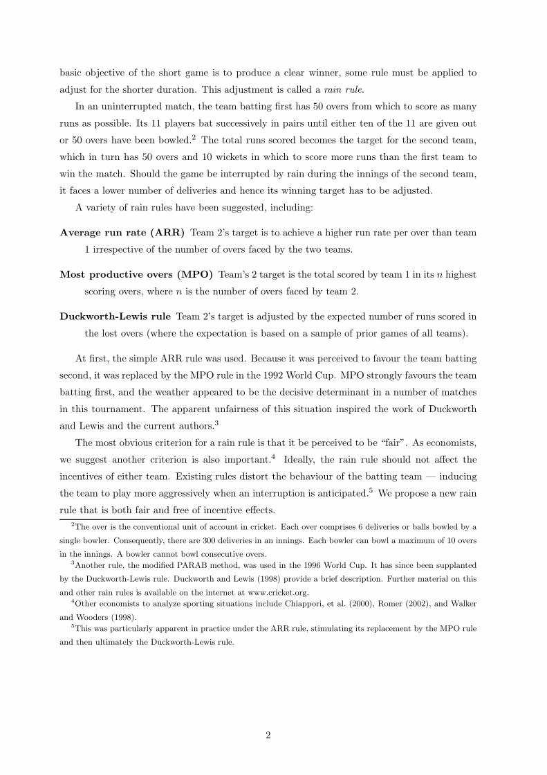
Figure 1: Expected runs Z(n, 10) with 10 wickets in hand
1 The Duckworth-Lewis rule
Currently, the most widely used rain rule is that proposed by Duckworth and Lewis, introduced
in 1997. It was applied in the 1999 World Cup in England, and is now used almost universally.
Using data from a large number of past matches, Duckworth and Lewis estimated the expo-
nential decay function
Z(n,w) = A(w)(1 − e−b(w)n)
where Z is the number of runs scored with n overs and w wickets remaining.6 The estimated
function is then tabulated, and the tables used to calculate the necessary adjustment in the
target. We believe it is more insightful to present the Duckworth-Lewis rule graphically.7
Application of the Duckworth-Lewis rule is most straightforward when the target is equal to
the average number of runs scored in one-day internationals (223). Figure 1 shows the expected
number of runs as a function of overs assuming no wickets have been lost, as estimated from the
data. It is the graph of the estimated function Z(n, 10).
Consider 3 different scenarios, in each of which there is a single interruption of 20 overs.
Interruption at the beginning — 30 overs remaining The average number of runs scored
with 30 overs and 10 wickets remaining is 172. This becomes the revised target required
of the second team to win the match.
Interruption at the end — last 20 overs lost The average number of runs scored in the
last 20 overs (assuming 10 wickets intact) is 131. The interruption costs the second team
the opportunity to score these runs, so that the target is reduced by 131 runs. The revised6Duckworth and Lewis (1998) use w to denote wickets lost rather than wickets remaining. They did not
publish their estimated parameters claiming commercial sensitivity. However, we have been able to reconstruct
their estimates from the published tables.7Adjustment is more complicated when there is an interruption in the first innings. For this reason, we confine
our attention to second innings interruptions in this paper.
3
10 20 30 50
255075
100125150175
72
120
152
187
Overs remaining
ExpectedRuns
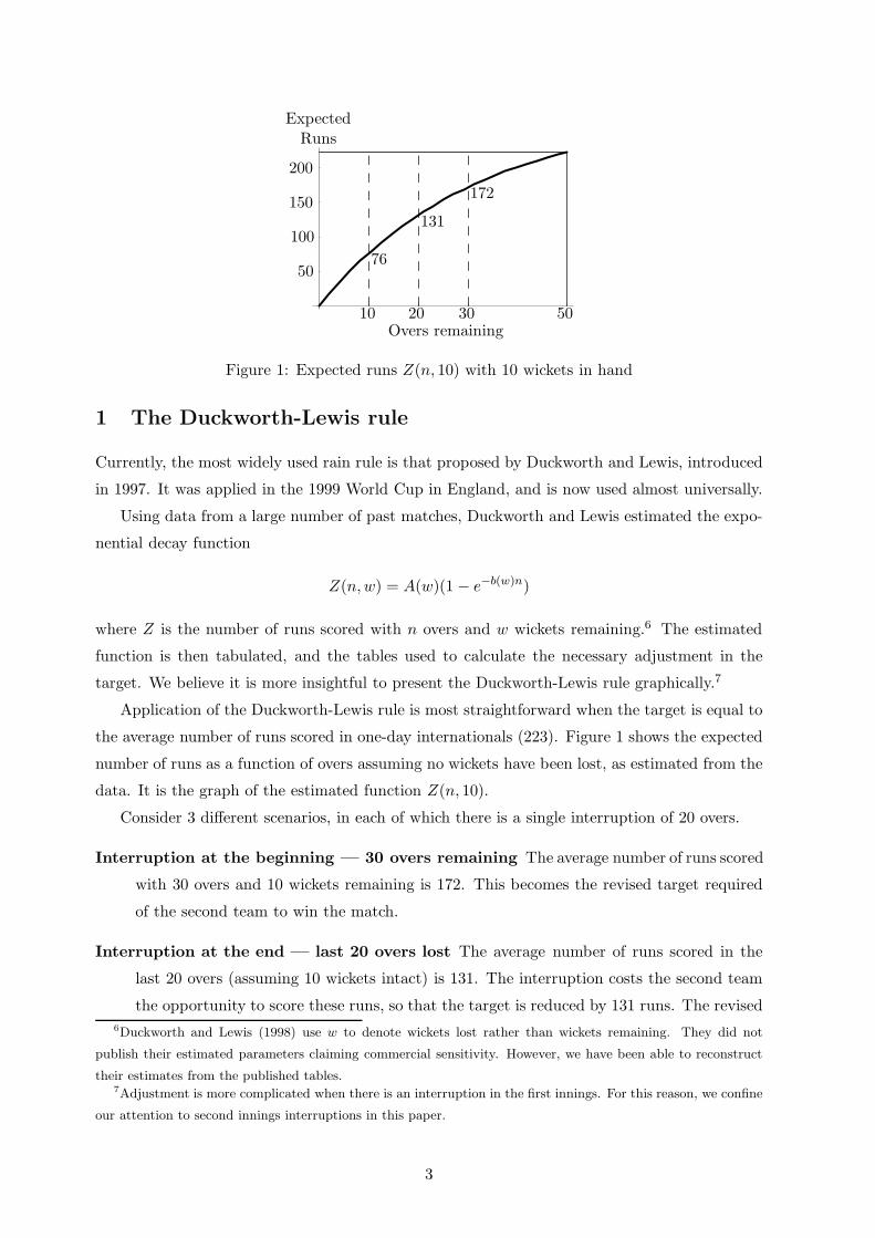
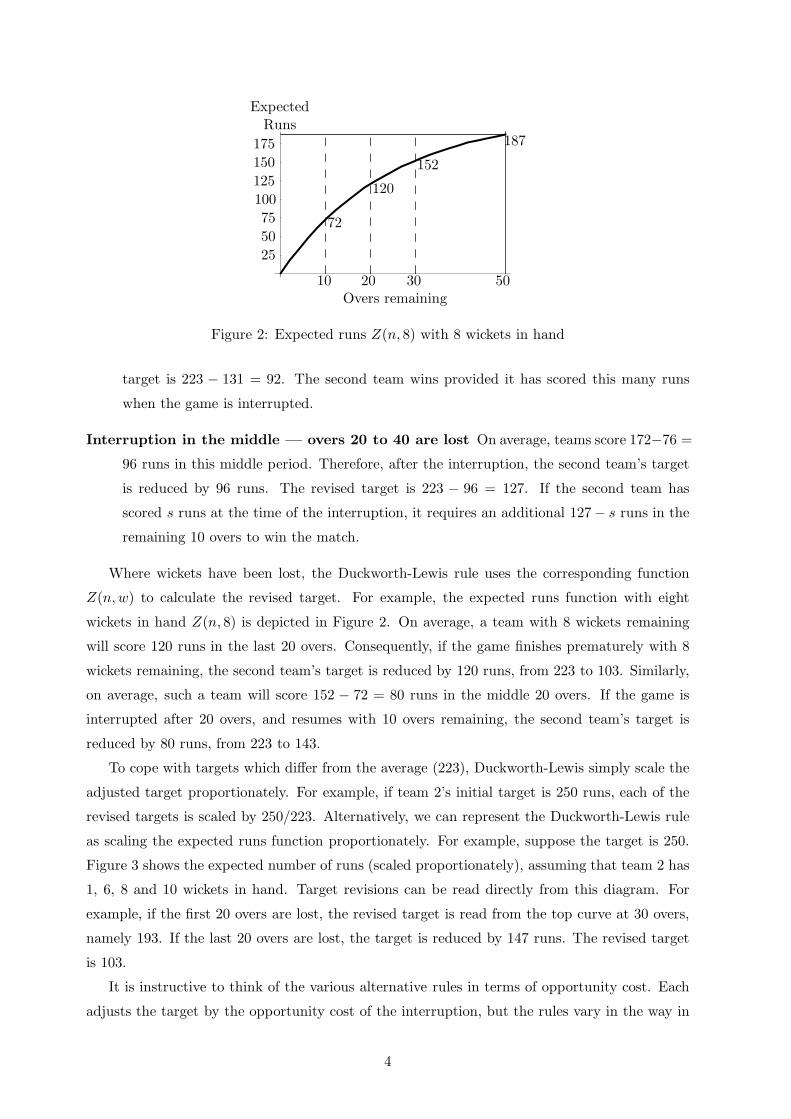
Figure 2: Expected runs Z(n, 8) with 8 wickets in hand
target is 223 − 131 = 92. The second team wins provided it has scored this many runs
when the game is interrupted.
Interruption in the middle — overs 20 to 40 are lost On average, teams score 172−76 =
96 runs in this middle period. Therefore, after the interruption, the second team’s target
is reduced by 96 runs. The revised target is 223 − 96 = 127. If the second team has
scored s runs at the time of the interruption, it requires an additional 127− s runs in the
remaining 10 overs to win the match.
Where wickets have been lost, the Duckworth-Lewis rule uses the corresponding function
Z(n,w) to calculate the revised target. For example, the expected runs function with eight
wickets in hand Z(n, 8) is depicted in Figure 2. On average, a team with 8 wickets remaining
will score 120 runs in the last 20 overs. Consequently, if the game finishes prematurely with 8
wickets remaining, the second team’s target is reduced by 120 runs, from 223 to 103. Similarly,
on average, such a team will score 152 − 72 = 80 runs in the middle 20 overs. If the game is
interrupted after 20 overs, and resumes with 10 overs remaining, the second team’s target is
reduced by 80 runs, from 223 to 143.
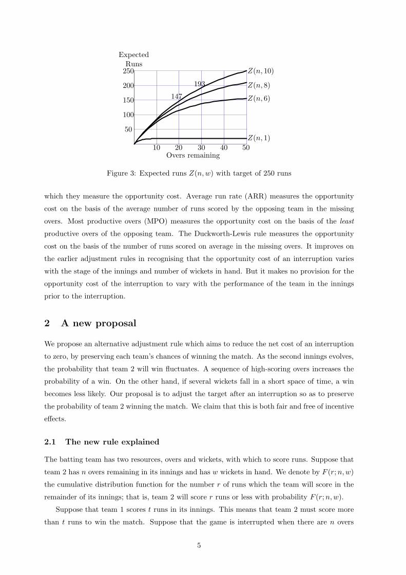
To cope with targets which differ from the average (223), Duckworth-Lewis simply scale the
adjusted target proportionately. For example, if team 2’s initial target is 250 runs, each of the
revised targets is scaled by 250/223. Alternatively, we can represent the Duckworth-Lewis rule
as scaling the expected runs function proportionately. For example, suppose the target is 250.
Figure 3 shows the expected number of runs (scaled proportionately), assuming that team 2 has
1, 6, 8 and 10 wickets in hand. Target revisions can be read directly from this diagram. For
example, if the first 20 overs are lost, the revised target is read from the top curve at 30 overs,
namely 193. If the last 20 overs are lost, the target is reduced by 147 runs. The revised target
is 103.
It is instructive to think of the various alternative rules in terms of opportunity cost. Each
adjusts the target by the opportunity cost of the interruption, but the rules vary in the way in
4
10 20 30 40 50
50
100
150
200
250
193
147
Z(n, 10)
Z(n, 8)
Z(n, 6)
Z(n, 1)
Overs remaining
ExpectedRuns
Figure 3: Expected runs Z(n,w) with target of 250 runs
which they measure the opportunity cost. Average run rate (ARR) measures the opportunity
cost on the basis of the average number of runs scored by the opposing team in the missing
overs. Most productive overs (MPO) measures the opportunity cost on the basis of the least
productive overs of the opposing team. The Duckworth-Lewis rule measures the opportunity
cost on the basis of the number of runs scored on average in the missing overs. It improves on
the earlier adjustment rules in recognising that the opportunity cost of an interruption varies
with the stage of the innings and number of wickets in hand. But it makes no provision for the
opportunity cost of the interruption to vary with the performance of the team in the innings
prior to the interruption.
2 A new proposal
We propose an alternative adjustment rule which aims to reduce the net cost of an interruption
to zero, by preserving each team’s chances of winning the match. As the second innings evolves,
the probability that team 2 will win fluctuates. A sequence of high-scoring overs increases the
probability of a win. On the other hand, if several wickets fall in a short space of time, a win
becomes less likely. Our proposal is to adjust the target after an interruption so as to preserve
the probability of team 2 winning the match. We claim that this is both fair and free of incentive
effects.
2.1 The new rule explained
The batting team has two resources, overs and wickets, with which to score runs. Suppose that
team 2 has n overs remaining in its innings and has w wickets in hand. We denote by F (r;n,w)
the cumulative distribution function for the number r of runs which the team will score in the
remainder of its innings; that is, team 2 will score r runs or less with probability F (r;n,w).
Suppose that team 1 scores t runs in its innings. This means that team 2 must score more
than t runs to win the match. Suppose that the game is interrupted when there are n overs
5
nn′
Reduction in target
A
BC
Overs remaining
Runsrequired
Wormt − st′ − s
D
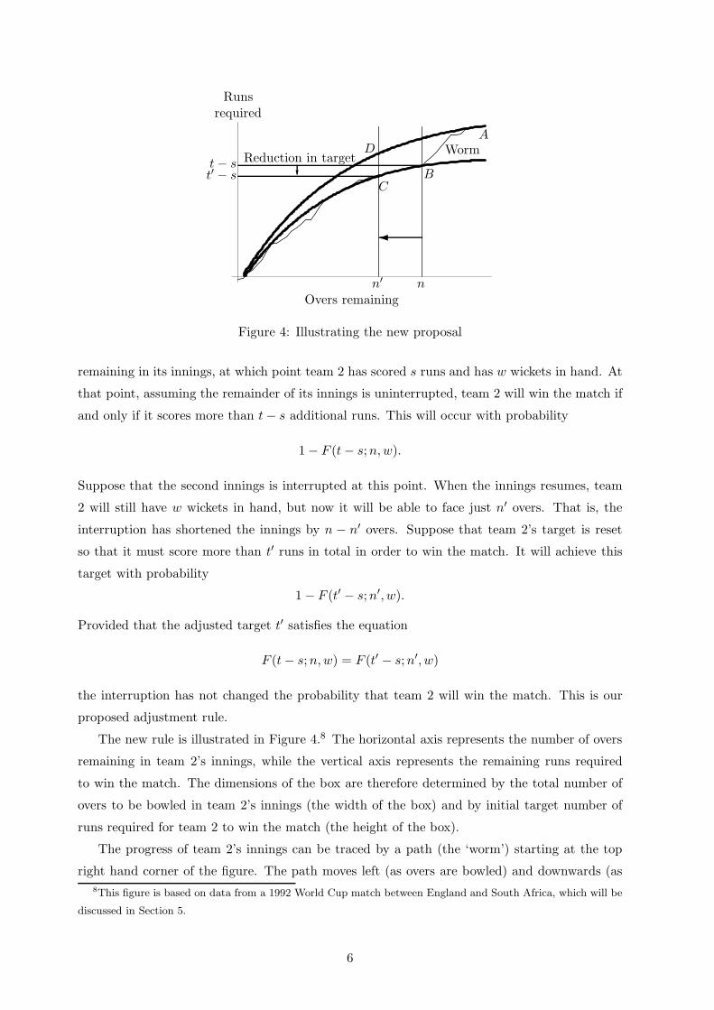
Figure 4: Illustrating the new proposal
remaining in its innings, at which point team 2 has scored s runs and has w wickets in hand. At
that point, assuming the remainder of its innings is uninterrupted, team 2 will win the match if
and only if it scores more than t − s additional runs. This will occur with probability
1 − F (t − s;n,w).
Suppose that the second innings is interrupted at this point. When the innings resumes, team
2 will still have w wickets in hand, but now it will be able to face just n′ overs. That is, the
interruption has shortened the innings by n − n′ overs. Suppose that team 2’s target is reset
so that it must score more than t′ runs in total in order to win the match. It will achieve this
target with probability
1 − F (t′ − s;n′, w).
Provided that the adjusted target t′ satisfies the equation
F (t − s;n,w) = F (t′ − s;n′, w)
the interruption has not changed the probability that team 2 will win the match. This is our
proposed adjustment rule.
The new rule is illustrated in Figure 4.8 The horizontal axis represents the number of overs
remaining in team 2’s innings, while the vertical axis represents the remaining runs required
to win the match. The dimensions of the box are therefore determined by the total number of
overs to be bowled in team 2’s innings (the width of the box) and by initial target number of
runs required for team 2 to win the match (the height of the box).
The progress of team 2’s innings can be traced by a path (the ‘worm’) starting at the top
right hand corner of the figure. The path moves left (as overs are bowled) and downwards (as8This figure is based on data from a 1992 World Cup match between England and South Africa, which will be
discussed in Section 5.
6
runs are scored). Provided the innings is not interrupted, this curve must eventually reach either
the left or the bottom boundary of the box. If it terminates on the bottom boundary, team 2
wins the game since it has achieved its target. On the other hand, if the curve terminates on
the left boundary, team 2 has failed to achieve its target in the allotted number of overs. If the
curve reaches the point (0,1), the game is a draw. Otherwise, team 1 wins the match.
The smooth curves are iso-probability loci, the shape of which varies with the number of
wickets in hand. The top curve connecting the bottom-left and top-right corners of the box is
the initial iso-probability of victory curve. At each point on this curve, team 2 has the same
probability of winning the match and this equals the probability of victory as measured at the
start of the second innings. If, as shown here, the ‘worm’ moves below this curve (from point
A to point B), team 2 is becoming more likely to win the match; if it moves above this curve,
team 2 is becoming less likely to win.
Suppose that the second innings is interrupted at point B, when n overs remain and the
score is s. When play resumes, the innings is shortened to n′ overs. The curve connecting the
origin and point B is another iso-probability curve, this time corresponding to the probability
measured immediately before the interruption. Under our proposal, the game is restarted at
point C — the point on the new iso-probability curve where n′ overs remain in the innings, so
that the probability of team 2 winning the match is unaffected by the interruption. That is, the
revised target is set at t′, where (n′, t′ − s) are the coordinates of point C.
Our proposal differs from the existing alternatives in two respects:
Quantity preserved The quantity preserved is the probability of winning, rather than the
required run rate (ARR) or the expected number of runs (Duckworth-Lewis).
Point of preservation This quantity is preserved at its value at the point of interruption,
rather than its value at the beginning of the match.9 In this way, the revised target takes
account of team 2’s performance prior to the interruption. A good start to the second
innings is not punished by an interruption. Similarly, an interruption does not allow team
2 to escape the consequences of a poor start.
The impact of this fundamental difference can be illustrated by the following hypothetical
but plausible example. Suppose that team 2, chasing 250 runs, gets off to a flying start and
scores 143 without loss in the first 20 overs.10 Clearly, at this point, team 2 is in a strong
position and has a high probability of winning. But, victory is not certain. The match is not
over and fortunes may change.
Now, suppose the game is interrupted by rain, and 20 overs are lost. When play resumes,
only 10 overs remain. Under the ARR rule, team 2’s target would be reduced to 150 off 309Analogous to ARR and Duckworth-Lewis, restarting the game at point D would preserve the probability of
winning at the start of the game, taking no account of team 2’s performance prior to the interruption.10Chasing a target of 214, South Africa reached 143 without loss in the 21st over in their match against
Zimbabwe on 28 September 1999.
7
overs. Having scored 143, play resumes with team 2 requiring only 7 runs off 10 overs. Victory
is almost assured. Under the Duckworth-Lewis rule, victory is fully assured. The revised target
is 143 and team 2 is declared the winner without batting again. Neither of these adjustments
seems fair.
Indeed, based on the estimates presented later in the paper, we calculate that team 2 has
a 98.8 percent chance of winning when the game is interrupted. To preserve this probability,
team 2 should be set the task of scoring 61 runs off the last 10 overs (with 10 wickets in hand)
to win the match. Not only is this fair, it would make the remainder of the game much more
entertaining.
To make the point in another way, consider the fates of two teams chasing identical targets.
Suppose that their games are interrupted after 20 overs, at which point team A has scored 20
more runs than team B. Suppose further that 20 overs are lost due to rain. Under the existing
rules, when play resumes, team B will still have to score 20 more runs than A to win their match,
but now with only 10 overs in which to do it. The interruption weighs differently on teams A
and B. When there are 30 overs remaining a 20 run difference is not particularly significant,
but it becomes very significant with only 10 overs to go.
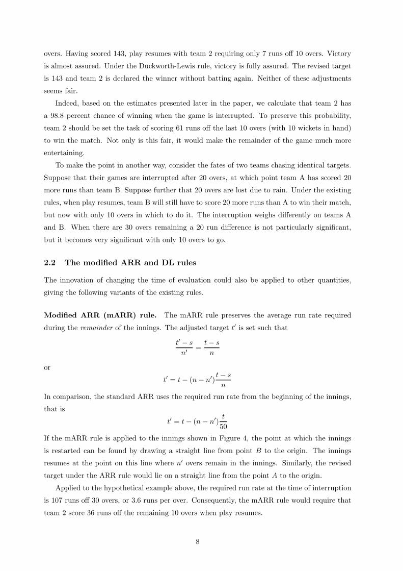
2.2 The modified ARR and DL rules
The innovation of changing the time of evaluation could also be applied to other quantities,
giving the following variants of the existing rules.
Modified ARR (mARR) rule. The mARR rule preserves the average run rate required
during the remainder of the innings. The adjusted target t′ is set such that
t′ − s
n′ =t − s
n
or
t′ = t − (n − n′)t − s
n
In comparison, the standard ARR uses the required run rate from the beginning of the innings,
that is
t′ = t − (n − n′)t
50
If the mARR rule is applied to the innings shown in Figure 4, the point at which the innings
is restarted can be found by drawing a straight line from point B to the origin. The innings
resumes at the point on this line where n′ overs remain in the innings. Similarly, the revised
target under the ARR rule would lie on a straight line from the point A to the origin.
Applied to the hypothetical example above, the required run rate at the time of interruption
is 107 runs off 30 overs, or 3.6 runs per over. Consequently, the mARR rule would require that
team 2 score 36 runs off the remaining 10 overs when play resumes.
8
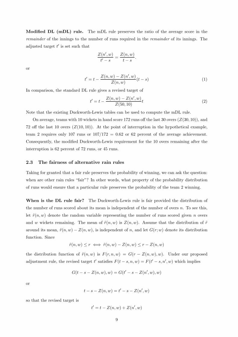
Modified DL (mDL) rule. The mDL rule preserves the ratio of the average score in the
remainder of the innings to the number of runs required in the remainder of its innings. The
adjusted target t′ is set such that
Z(n′, w)t′ − s
=Z(n,w)t − s
.
or
t′ = t − Z(n,w) − Z(n′, w)Z(n,w)
(t − s) (1)
In comparison, the standard DL rule gives a revised target of
t′ = t − Z(n,w) − Z(n′, w)Z(50, 10)
t (2)
Note that the existing Duckworth-Lewis tables can be used to compute the mDL rule.
On average, teams with 10 wickets in hand score 172 runs off the last 30 overs (Z(30, 10)), and
72 off the last 10 overs (Z(10, 10)). At the point of interruption in the hypothetical example,
team 2 requires only 107 runs or 107/172 = 0.62 or 62 percent of the average achievement.
Consequently, the modified Duckworth-Lewis requirement for the 10 overs remaining after the
interruption is 62 percent of 72 runs, or 45 runs.
2.3 The fairness of alternative rain rules
Taking for granted that a fair rule preserves the probability of winning, we can ask the question:
when are other rain rules “fair”? In other words, what property of the probability distribution
of runs would ensure that a particular rule preserves the probability of the team 2 winning.
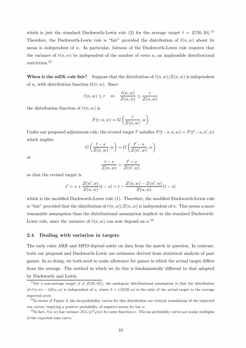
When is the DL rule fair? The Duckworth-Lewis rule is fair provided the distribution of
the number of runs scored about its mean is independent of the number of overs n. To see this,
let r̃(n,w) denote the random variable representing the number of runs scored given n overs
and w wickets remaining. The mean of r̃(n,w) is Z(n,w). Assume that the distribution of r̃
around its mean, r̃(n,w) − Z(n,w), is independent of n, and let G(r;w) denote its distribution
function. Since
r̃(n,w) ≤ r ⇐⇒ r̃(n,w) − Z(n,w) ≤ r − Z(n,w)
the distribution function of r̃(n,w) is F (r, n,w) = G(r − Z(n,w), w). Under our proposed
adjustment rule, the revised target t′ satisfies F (t − s, n,w) = F (t′ − s, n′, w) which implies
G(t − s − Z(n,w), w) = G(t′ − s − Z(n′, w), w)
or
t − s − Z(n,w) = t′ − s − Z(n′, w)
so that the revised target is
t′ = t − Z(n,w) + Z(n′, w)
9
which is just the standard Duckworth-Lewis rule (2) for the average target t = Z(50, 10).11
Therefore, the Duckworth-Lewis rule is “fair” provided the distribution of r̃(n,w) about its
mean is independent of n. In particular, fairness of the Duckworth-Lewis rule requires that
the variance of r̃(n,w) be independent of the number of overs n, an implausible distributional
restriction.12
When is the mDL rule fair? Suppose that the distribution of r̃(n,w)/Z(n,w) is independent
of n, with distribution function G(r;w). Since
r̃(n,w) ≤ r ⇔ r̃(n,w)Z(n,w)
≤ r
Z(n,w)
the distribution function of r̃(n,w) is
F (r, n,w) = G
(r
Z(n,w), w
)
Under our proposed adjustment rule, the revised target t′ satisfies F (t−s, n,w) = F (t′−s, n′, w)
which implies
G
(t − s
Z(n,w), w
)= G
(t′ − s
Z(n′, w), w
)
ort − s
Z(n,w)=
t′ − s
Z(n′, w)
so that the revised target is
t′ = s +Z(n′, w)Z(n,w)
(t − s) = t − Z(n,w) − Z(n′, w)Z(n,w)
(t − s)
which is the modified Duckworth-Lewis rule (1). Therefore, the modified Duckworth-Lewis rule
is “fair” provided that the distribution of r̃(n,w)/Z(n,w) is independent of n. This seems a more
reasonable assumption than the distributional assumption implicit in the standard Duckworth-
Lewis rule, since the variance of r̃(n,w) can now depend on n.13
2.4 Dealing with variation in targets
The early rules ARR and MPO depend solely on data from the match in question. In contrast,
both our proposal and Duckworth-Lewis use estimates derived from statistical analysis of past
games. In so doing, we both need to make allowance for games in which the actual target differs
from the average. The method in which we do this is fundamentally different to that adopted
by Duckworth and Lewis.11For a non-average target (t �= Z(50, 10)), the analogous distributional assumption is that the distribution
of r̃(n, w) − λZ(n, w) is independent of n, where λ = t/Z(50, w) is the ratio of the actual target to the average
expected score.12In terms of Figure 4, the iso-probability curves for this distribution are vertical translations of the expected
run curves, implying a positive probability of negative scores for low n.13In fact, r̃(n, w) has variance Z(n, w)2ϕ(w) for some function w. The iso-probability curves are scalar multiples
of the expected runs curve.
10
To compute the opportunity cost of an interruption, Duckworth and Lewis scale the average
number of runs scored in the lost overs Z(n,w)− Z(n′, w) by the ratio of the actual target t to
the average target Z(50, 10). In so doing, they effectively ascribe all the variation of the actual
score from the average to the “quality of the pitch”. We do precisely the opposite — all variation
in scores is assumed to be entirely due to chance or superior performance of the opposing team.
While undoubtedly all three factors — pitch, teams’ ability and performance, and luck —
contribute to the total scored by team 1 and hence the target facing team 2, it is impossible
to determine the relative contribution of these factors. Consequently, we refrain from making
any adjustment in the rule to allow for targets which differ from average. In defence of this
decision, we note that it is the shapes of the iso-probability contours and not their levels which
are relevant in determining the revised target. Provided that the shapes of these contours do
not vary systematically with either the quality of the pitch or the performance and ability of the
teams, our conclusions regarding fairness and incentives will not be undermined by variation in
target scores.
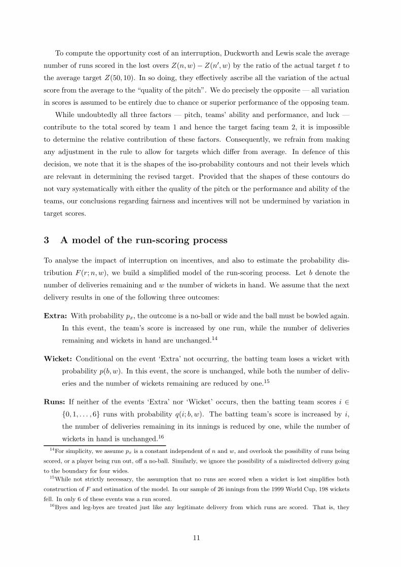
3 A model of the run-scoring process
To analyse the impact of interruption on incentives, and also to estimate the probability dis-
tribution F (r;n,w), we build a simplified model of the run-scoring process. Let b denote the
number of deliveries remaining and w the number of wickets in hand. We assume that the next
delivery results in one of the following three outcomes:
Extra: With probability px, the outcome is a no-ball or wide and the ball must be bowled again.
In this event, the team’s score is increased by one run, while the number of deliveries
remaining and wickets in hand are unchanged.14
Wicket: Conditional on the event ‘Extra’ not occurring, the batting team loses a wicket with
probability p(b, w). In this event, the score is unchanged, while both the number of deliv-
eries and the number of wickets remaining are reduced by one.15
Runs: If neither of the events ‘Extra’ nor ‘Wicket’ occurs, then the batting team scores i ∈{0, 1, . . . , 6} runs with probability q(i; b, w). The batting team’s score is increased by i,
the number of deliveries remaining in its innings is reduced by one, while the number of
wickets in hand is unchanged.16
14For simplicity, we assume px is a constant independent of n and w, and overlook the possibility of runs being
scored, or a player being run out, off a no-ball. Similarly, we ignore the possibility of a misdirected delivery going
to the boundary for four wides.15While not strictly necessary, the assumption that no runs are scored when a wicket is lost simplifies both
construction of F and estimation of the model. In our sample of 26 innings from the 1999 World Cup, 198 wickets
fell. In only 6 of these events was a run scored.16Byes and leg-byes are treated just like any legitimate delivery from which runs are scored. That is, they
11
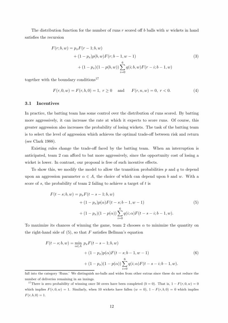
The distribution function for the number of runs r scored off b balls with w wickets in hand
satisfies the recursion
F (r; b, w) = pxF (r − 1; b, w)
+ (1 − px)p(b, w)F (r; b − 1, w − 1) (3)
+ (1 − px)(1 − p(b, w))6∑
i=0
q(i; b, w)F (r − i; b − 1, w)
together with the boundary conditions17
F (r, 0, w) = F (r, b, 0) = 1, r ≥ 0 and F (r, n,w) = 0, r < 0. (4)
3.1 Incentives
In practice, the batting team has some control over the distribution of runs scored. By batting
more aggressively, it can increase the rate at which it expects to score runs. Of course, this
greater aggression also increases the probability of losing wickets. The task of the batting team
is to select the level of aggression which achieves the optimal trade-off between risk and return
(see Clark 1988).
Existing rules change the trade-off faced by the batting team. When an interruption is
anticipated, team 2 can afford to bat more aggressively, since the opportunity cost of losing a
wicket is lower. In contrast, our proposal is free of such incentive effects.
To show this, we modify the model to allow the transition probabilities p and q to depend
upon an aggression parameter α ∈ A, the choice of which can depend upon b and w. With a
score of s, the probability of team 2 failing to achieve a target of t is
F (t − s; b, w) = pxF (t − s − 1; b, w)
+ (1 − px)p(α)F (t − s; b − 1, w − 1) (5)
+ (1 − px)(1 − p(α))6∑
i=0
q(i;α)F (t − s − i; b − 1, w).
To maximize its chances of winning the game, team 2 chooses α to minimize the quantity on
the right-hand side of (5), so that F satisfies Bellman’s equation
F (t − s; b, w) = minα∈A
pxF (t − s − 1; b, w)
+ (1 − px)p(α)F (t − s; b − 1, w − 1) (6)
+ (1 − px)(1 − p(α))6∑
i=0
q(i;α)F (t − s − i; b − 1, w).
fall into the category ‘Runs.’ We distinguish no-balls and wides from other extras since these do not reduce the
number of deliveries remaining in an innings.17There is zero probability of winning once 50 overs have been completed (b = 0). That is, 1 − F (r, 0, w) = 0
which implies F (r, 0, w) = 1. Similarly, when 10 wickets have fallen (w = 0), 1 − F (r, b, 0) = 0 which implies
F (r, b, 0) = 1.
12
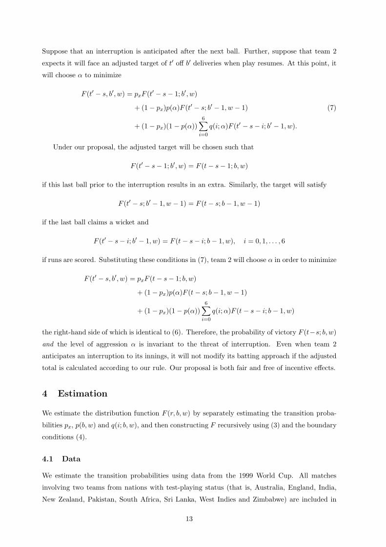
Suppose that an interruption is anticipated after the next ball. Further, suppose that team 2
expects it will face an adjusted target of t′ off b′ deliveries when play resumes. At this point, it
will choose α to minimize
F (t′ − s, b′, w) = pxF (t′ − s − 1; b′, w)
+ (1 − px)p(α)F (t′ − s; b′ − 1, w − 1) (7)
+ (1 − px)(1 − p(α))6∑
i=0
q(i;α)F (t′ − s − i; b′ − 1, w).
Under our proposal, the adjusted target will be chosen such that
F (t′ − s − 1; b′, w) = F (t − s − 1; b, w)
if this last ball prior to the interruption results in an extra. Similarly, the target will satisfy
F (t′ − s; b′ − 1, w − 1) = F (t − s; b − 1, w − 1)
if the last ball claims a wicket and
F (t′ − s − i; b′ − 1, w) = F (t − s − i; b − 1, w), i = 0, 1, . . . , 6
if runs are scored. Substituting these conditions in (7), team 2 will choose α in order to minimize
F (t′ − s, b′, w) = pxF (t − s − 1; b, w)
+ (1 − px)p(α)F (t − s; b − 1, w − 1)
+ (1 − px)(1 − p(α))6∑
i=0
q(i;α)F (t − s − i; b − 1, w)
the right-hand side of which is identical to (6). Therefore, the probability of victory F (t−s; b, w)
and the level of aggression α is invariant to the threat of interruption. Even when team 2
anticipates an interruption to its innings, it will not modify its batting approach if the adjusted
total is calculated according to our rule. Our proposal is both fair and free of incentive effects.
4 Estimation
We estimate the distribution function F (r, b, w) by separately estimating the transition proba-
bilities px, p(b, w) and q(i; b, w), and then constructing F recursively using (3) and the boundary
conditions (4).
4.1 Data
We estimate the transition probabilities using data from the 1999 World Cup. All matches
involving two teams from nations with test-playing status (that is, Australia, England, India,
New Zealand, Pakistan, South Africa, Sri Lanka, West Indies and Zimbabwe) are included in
13
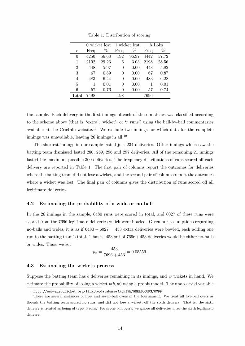
Table 1: Distribution of scoring
0 wicket lost 1 wicket lost All obsr Freq % Freq % Freq %0 4250 56.68 192 96.97 4442 57.721 2192 29.23 6 3.03 2198 28.562 448 5.97 0 0.00 448 5.823 67 0.89 0 0.00 67 0.874 483 6.44 0 0.00 483 6.285 1 0.01 0 0.00 1 0.016 57 0.76 0 0.00 57 0.74
Total 7498 198 7696
the sample. Each delivery in the first innings of each of these matches was classified according
to the scheme above (that is, ‘extra’, ‘wicket’, or ‘r runs’) using the ball-by-ball commentaries
available at the CricInfo website.18 We exclude two innings for which data for the complete
innings was unavailable, leaving 26 innings in all.19
The shortest innings in our sample lasted just 234 deliveries. Other innings which saw the
batting team dismissed lasted 280, 289, 296 and 297 deliveries. All of the remaining 21 innings
lasted the maximum possible 300 deliveries. The frequency distributions of runs scored off each
delivery are reported in Table 1. The first pair of columns report the outcomes for deliveries
where the batting team did not lose a wicket, and the second pair of columns report the outcomes
where a wicket was lost. The final pair of columns gives the distribution of runs scored off all
legitimate deliveries.
4.2 Estimating the probability of a wide or no-ball
In the 26 innings in the sample, 6480 runs were scored in total, and 6027 of these runs were
scored from the 7696 legitimate deliveries which were bowled. Given our assumptions regarding
no-balls and wides, it is as if 6480 − 6027 = 453 extra deliveries were bowled, each adding one
run to the batting team’s total. That is, 453 out of 7696+453 deliveries would be either no-balls
or wides. Thus, we set
px =453
7696 + 453= 0.05559.
4.3 Estimating the wickets process
Suppose the batting team has b deliveries remaining in its innings, and w wickets in hand. We
estimate the probability of losing a wicket p(b, w) using a probit model. The unobserved variable18http://www-aus.cricket.org/link to database/ARCHIVE/WORLD CUPS/WC9919There are several instances of five- and seven-ball overs in the tournament. We treat all five-ball overs as
though the batting team scored no runs, and did not lose a wicket, off the sixth delivery. That is, the sixth
delivery is treated as being of type ‘0 runs.’ For seven-ball overs, we ignore all deliveries after the sixth legitimate
delivery.
14
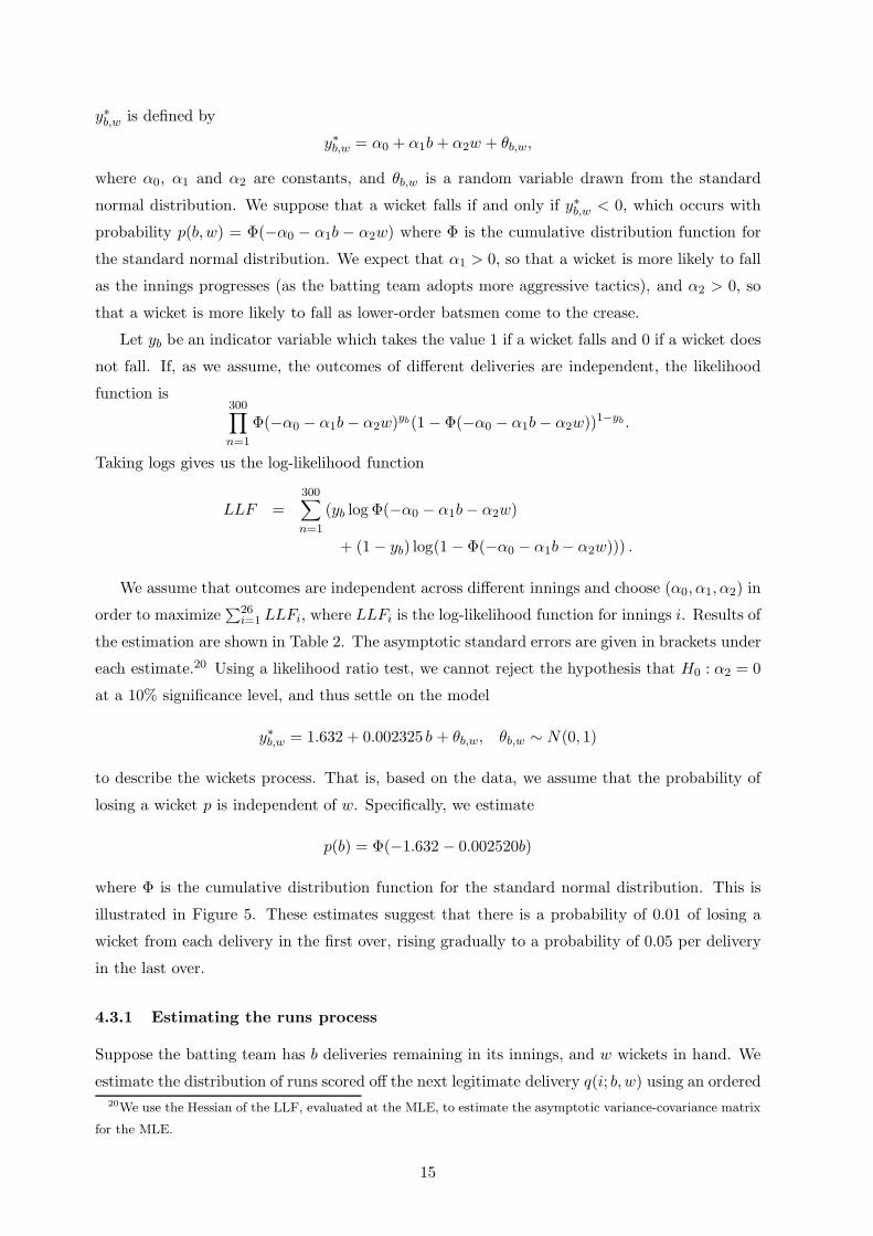
y∗b,w is defined by
y∗b,w = α0 + α1b + α2w + θb,w,
where α0, α1 and α2 are constants, and θb,w is a random variable drawn from the standard
normal distribution. We suppose that a wicket falls if and only if y∗b,w < 0, which occurs with
probability p(b, w) = Φ(−α0 − α1b − α2w) where Φ is the cumulative distribution function for
the standard normal distribution. We expect that α1 > 0, so that a wicket is more likely to fall
as the innings progresses (as the batting team adopts more aggressive tactics), and α2 > 0, so
that a wicket is more likely to fall as lower-order batsmen come to the crease.
Let yb be an indicator variable which takes the value 1 if a wicket falls and 0 if a wicket does
not fall. If, as we assume, the outcomes of different deliveries are independent, the likelihood
function is300∏n=1
Φ(−α0 − α1b − α2w)yb(1 − Φ(−α0 − α1b − α2w))1−yb .
Taking logs gives us the log-likelihood function
LLF =300∑n=1
(yb log Φ(−α0 − α1b − α2w)
+ (1 − yb) log(1 − Φ(−α0 − α1b − α2w))) .
We assume that outcomes are independent across different innings and choose (α0, α1, α2) in
order to maximize∑26
i=1 LLFi, where LLFi is the log-likelihood function for innings i. Results of
the estimation are shown in Table 2. The asymptotic standard errors are given in brackets under
each estimate.20 Using a likelihood ratio test, we cannot reject the hypothesis that H0 : α2 = 0
at a 10% significance level, and thus settle on the model
y∗b,w = 1.632 + 0.002325 b + θb,w, θb,w ∼ N(0, 1)
to describe the wickets process. That is, based on the data, we assume that the probability of
losing a wicket p is independent of w. Specifically, we estimate
p(b) = Φ(−1.632 − 0.002520b)
where Φ is the cumulative distribution function for the standard normal distribution. This is
illustrated in Figure 5. These estimates suggest that there is a probability of 0.01 of losing a
wicket from each delivery in the first over, rising gradually to a probability of 0.05 per delivery
in the last over.
4.3.1 Estimating the runs process
Suppose the batting team has b deliveries remaining in its innings, and w wickets in hand. We
estimate the distribution of runs scored off the next legitimate delivery q(i; b, w) using an ordered20We use the Hessian of the LLF, evaluated at the MLE, to estimate the asymptotic variance-covariance matrix
for the MLE.
15
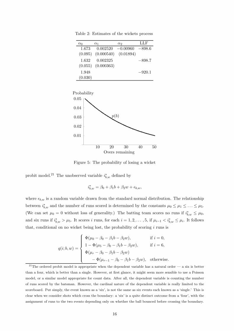
Table 2: Estimates of the wickets process
α0 α1 α2 LLF1.673 0.002520 −0.00960 −898.6
(0.095) (0.000540) (0.01894)1.632 0.002325 −898.7
(0.055) (0.000363)1.948 −920.1
(0.030)
10 20 30 40 50
0.01
0.02
0.03
0.04
0.05
Overs remaining
Probability
p(b)
Figure 5: The probability of losing a wicket
probit model.21 The unobserved variable i∗b,w defined by
i∗b,w = β0 + β1b + β2w + εb,w,
where εb,w is a random variable drawn from the standard normal distribution. The relationship
between i∗b,w and the number of runs scored is determined by the constants µ0 ≤ µ1 ≤ . . . ≤ µ5.
(We can set µ0 = 0 without loss of generality.) The batting team scores no runs if i∗b,w ≤ µ0,
and six runs if i∗b,w > µ5. It scores i runs, for each i = 1, 2, . . . , 5, if µi−1 < i∗b,w ≤ µi. It follows
that, conditional on no wicket being lost, the probability of scoring i runs is
q(i; b, w) =
Φ(µ0 − β0 − β1b − β2w), if i = 0,
1 − Φ(µ5 − β0 − β1b − β2w), if i = 6,
Φ(µr − β0 − β1b − β2w)
− Φ(µr−1 − β0 − β1b − β2w), otherwise.21The ordered probit model is appropriate when the dependent variable has a natural order — a six is better
than a four, which is better than a single. However, at first glance, it might seem more sensible to use a Poisson
model, or a similar model appropriate for count data. After all, the dependent variable is counting the number
of runs scored by the batsman. However, the cardinal nature of the dependent variable is really limited to the
scoreboard. Put simply, the event known as a ‘six’, is not the same as six events each known as a ‘single.’ This is
clear when we consider shots which cross the boundary: a ‘six’ is a quite distinct outcome from a ‘four’, with the
assignment of runs to the two events depending only on whether the ball bounced before crossing the boundary.
16
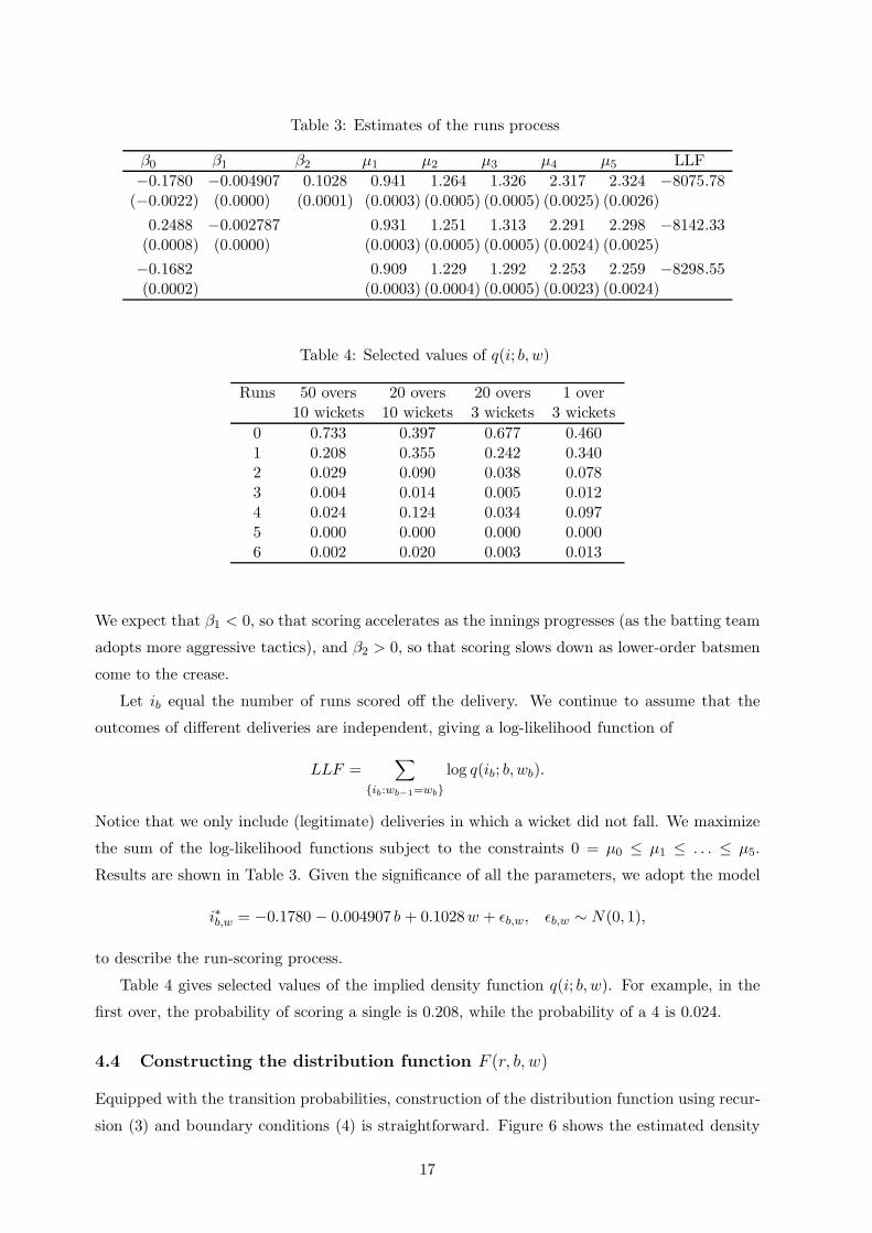
Table 3: Estimates of the runs process
β0 β1 β2 µ1 µ2 µ3 µ4 µ5 LLF−0.1780 −0.004907 0.1028 0.941 1.264 1.326 2.317 2.324 −8075.78
(−0.0022) (0.0000) (0.0001) (0.0003) (0.0005) (0.0005) (0.0025) (0.0026)0.2488 −0.002787 0.931 1.251 1.313 2.291 2.298 −8142.33(0.0008) (0.0000) (0.0003) (0.0005) (0.0005) (0.0024) (0.0025)−0.1682 0.909 1.229 1.292 2.253 2.259 −8298.55(0.0002) (0.0003) (0.0004) (0.0005) (0.0023) (0.0024)
Table 4: Selected values of q(i; b, w)
Runs 50 overs 20 overs 20 overs 1 over10 wickets 10 wickets 3 wickets 3 wickets
0 0.733 0.397 0.677 0.4601 0.208 0.355 0.242 0.3402 0.029 0.090 0.038 0.0783 0.004 0.014 0.005 0.0124 0.024 0.124 0.034 0.0975 0.000 0.000 0.000 0.0006 0.002 0.020 0.003 0.013
We expect that β1 < 0, so that scoring accelerates as the innings progresses (as the batting team
adopts more aggressive tactics), and β2 > 0, so that scoring slows down as lower-order batsmen
come to the crease.
Let ib equal the number of runs scored off the delivery. We continue to assume that the
outcomes of different deliveries are independent, giving a log-likelihood function of
LLF =∑
{ib:wb−1=wb}log q(ib; b, wb).
Notice that we only include (legitimate) deliveries in which a wicket did not fall. We maximize
the sum of the log-likelihood functions subject to the constraints 0 = µ0 ≤ µ1 ≤ . . . ≤ µ5.
Results are shown in Table 3. Given the significance of all the parameters, we adopt the model
i∗b,w = −0.1780 − 0.004907 b + 0.1028w + εb,w, εb,w ∼ N(0, 1),
to describe the run-scoring process.
Table 4 gives selected values of the implied density function q(i; b, w). For example, in the
first over, the probability of scoring a single is 0.208, while the probability of a 4 is 0.024.
4.4 Constructing the distribution function F (r, b, w)
Equipped with the transition probabilities, construction of the distribution function using recur-
sion (3) and boundary conditions (4) is straightforward. Figure 6 shows the estimated density
17
100 150 200 250 300 350
0.002
0.004
0.006
0.008
Figure 6: Distribution of total scores — estimated and actual
10 20 30 40 500
50
100
150
200
250
300
Overs remaining
Runsrequired
Figure 7: The contours of F (r; b, 10)
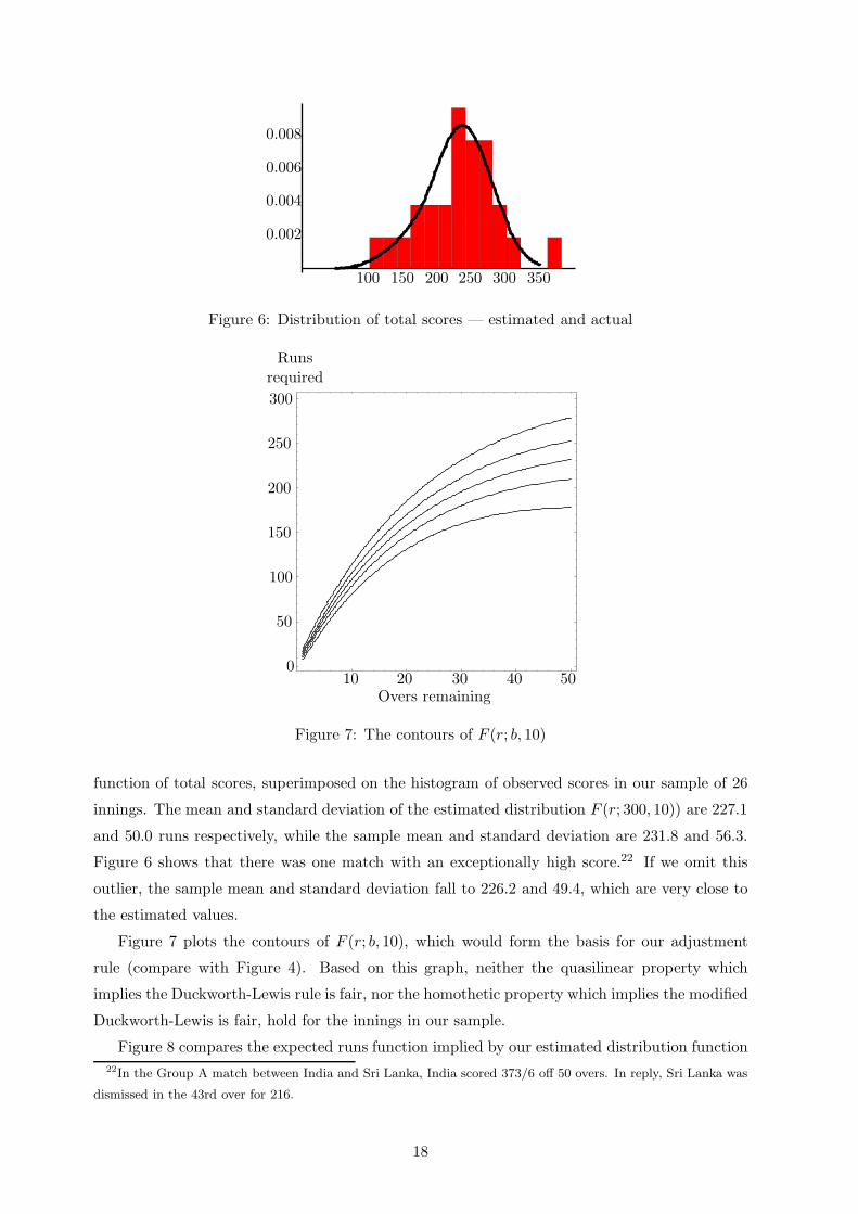
function of total scores, superimposed on the histogram of observed scores in our sample of 26
innings. The mean and standard deviation of the estimated distribution F (r; 300, 10)) are 227.1
and 50.0 runs respectively, while the sample mean and standard deviation are 231.8 and 56.3.
Figure 6 shows that there was one match with an exceptionally high score.22 If we omit this
outlier, the sample mean and standard deviation fall to 226.2 and 49.4, which are very close to
the estimated values.
Figure 7 plots the contours of F (r; b, 10), which would form the basis for our adjustment
rule (compare with Figure 4). Based on this graph, neither the quasilinear property which
implies the Duckworth-Lewis rule is fair, nor the homothetic property which implies the modified
Duckworth-Lewis is fair, hold for the innings in our sample.
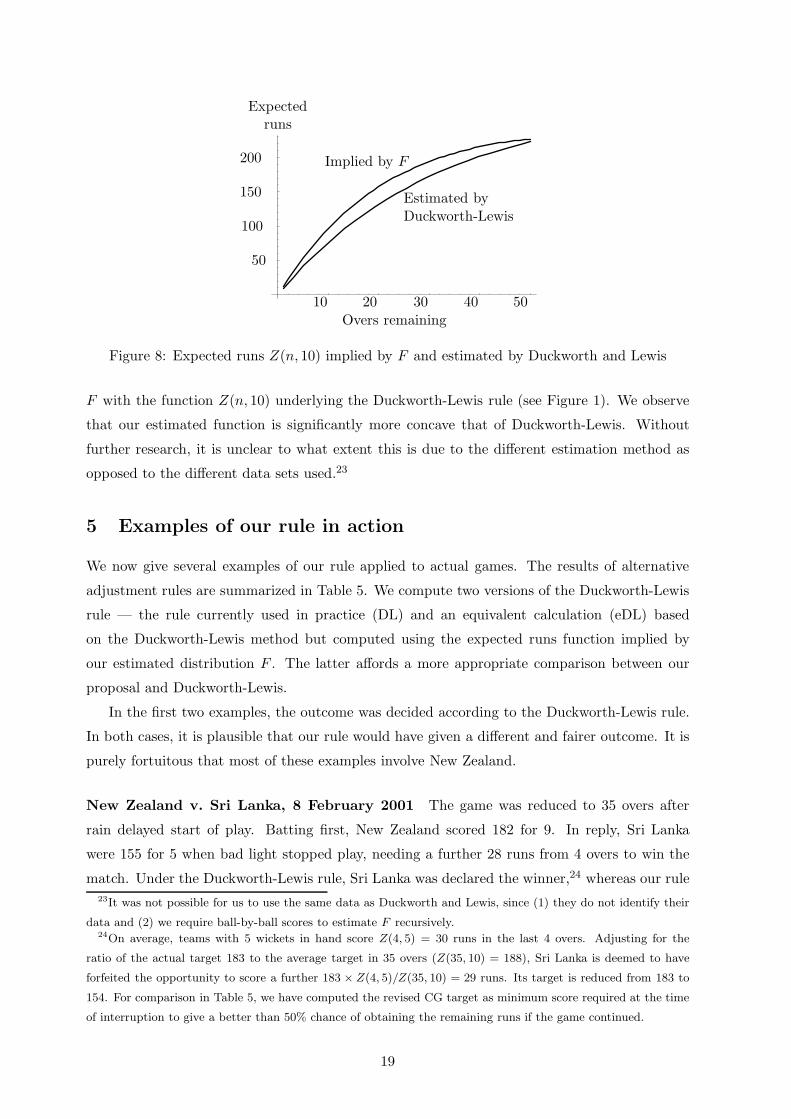
Figure 8 compares the expected runs function implied by our estimated distribution function22In the Group A match between India and Sri Lanka, India scored 373/6 off 50 overs. In reply, Sri Lanka was
dismissed in the 43rd over for 216.
18
10 20 30 40 50
50
100
150
200
Overs remaining
Expectedruns
Estimated byDuckworth-Lewis
Implied by F
Figure 8: Expected runs Z(n, 10) implied by F and estimated by Duckworth and Lewis
F with the function Z(n, 10) underlying the Duckworth-Lewis rule (see Figure 1). We observe
that our estimated function is significantly more concave that of Duckworth-Lewis. Without
further research, it is unclear to what extent this is due to the different estimation method as
opposed to the different data sets used.23
5 Examples of our rule in action
We now give several examples of our rule applied to actual games. The results of alternative
adjustment rules are summarized in Table 5. We compute two versions of the Duckworth-Lewis
rule — the rule currently used in practice (DL) and an equivalent calculation (eDL) based
on the Duckworth-Lewis method but computed using the expected runs function implied by
our estimated distribution F . The latter affords a more appropriate comparison between our
proposal and Duckworth-Lewis.
In the first two examples, the outcome was decided according to the Duckworth-Lewis rule.
In both cases, it is plausible that our rule would have given a different and fairer outcome. It is
purely fortuitous that most of these examples involve New Zealand.
New Zealand v. Sri Lanka, 8 February 2001 The game was reduced to 35 overs after
rain delayed start of play. Batting first, New Zealand scored 182 for 9. In reply, Sri Lanka
were 155 for 5 when bad light stopped play, needing a further 28 runs from 4 overs to win the
match. Under the Duckworth-Lewis rule, Sri Lanka was declared the winner,24 whereas our rule23It was not possible for us to use the same data as Duckworth and Lewis, since (1) they do not identify their
data and (2) we require ball-by-ball scores to estimate F recursively.24On average, teams with 5 wickets in hand score Z(4, 5) = 30 runs in the last 4 overs. Adjusting for the
ratio of the actual target 183 to the average target in 35 overs (Z(35, 10) = 188), Sri Lanka is deemed to have
forfeited the opportunity to score a further 183 × Z(4, 5)/Z(35, 10) = 29 runs. Its target is reduced from 183 to
154. For comparison in Table 5, we have computed the revised CG target as minimum score required at the time
of interruption to give a better than 50% chance of obtaining the remaining runs if the game continued.
19
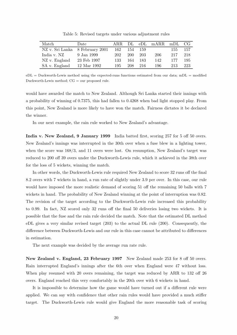
Table 5: Revised targets under various adjustment rules
Match Date ARR DL eDL mARR mDL CGNZ v. Sri Lanka 8 February 2001 162 154 159 155 157India v. NZ 9 Jan 1999 202 200 203 206 217 218NZ v. England 23 Feb 1997 133 164 183 142 177 195SA v. England 12 Mar 1992 195 208 216 196 213 223
eDL = Duckworth-Lewis method using the expected-runs functions estimated from our data; mDL = modified
Duckworth-Lewis method; CG = our proposed rule.
would have awarded the match to New Zealand. Although Sri Lanka started their innings with
a probability of winning of 0.7375, this had fallen to 0.4268 when bad light stopped play. From
this point, New Zealand is more likely to have won the match. Fairness dictates it be declared
the winner.
In our next example, the rain rule worked to New Zealand’s advantage.
India v. New Zealand, 9 January 1999 India batted first, scoring 257 for 5 off 50 overs.
New Zealand’s innings was interrupted in the 30th over when a fuse blew in a lighting tower,
when the score was 168/3, and 11 overs were lost. On resumption, New Zealand’s target was
reduced to 200 off 39 overs under the Duckworth-Lewis rule, which it achieved in the 38th over
for the loss of 5 wickets, winning the match.
In other words, the Duckworth-Lewis rule required New Zealand to score 32 runs off the final
8.2 overs with 7 wickets in hand, a run rate of slightly under 3.9 per over. In this case, our rule
would have imposed the more realistic demand of scoring 51 off the remaining 50 balls with 7
wickets in hand. The probability of New Zealand winning at the point of interruption was 0.82.
The revision of the target according to the Duckworth-Lewis rule increased this probability
to 0.99. In fact, NZ scored only 32 runs off the final 50 deliveries losing two wickets. It is
possible that the fuse and the rain rule decided the match. Note that the estimated DL method
eDL gives a very similar revised target (203) to the actual DL rule (200). Consequently, the
difference between Duckworth-Lewis and our rule in this case cannot be attributed to differences
in estimation.
The next example was decided by the average run rate rule.
New Zealand v. England, 23 February 1997 New Zealand made 253 for 8 off 50 overs.
Rain interrupted England’s innings after the 6th over when England were 47 without loss.
When play resumed with 20 overs remaining, the target was reduced by ARR to 132 off 26
overs. England reached this very comfortably in the 20th over with 6 wickets in hand.
It is impossible to determine how the game would have turned out if a different rule were
applied. We can say with confidence that other rain rules would have provided a much stiffer
target. The Duckworth-Lewis rule would give England the more reasonable task of scoring
20
164 − 47 = 117 off the last 20 overs with 10 wickets in hand (6 runs per over). Our rule would
increase this task to 195−47 = 148 runs off 20 overs (7.4 runs per over). While this may appear
an unreasonable target, it recognizes England’s commanding position having all ten wickets in
hand. At the beginning of their innings, England’s chances of winning the match are only 0.30.
Their excellent start increases this to 0.64 at the point of interruption. The CG rule preserves
this probability, while the Duckworth-Lewis rule increases the probability of winning to 0.94.
England would obtain a significant boost from the Duckworth-Lewis rule.
Our final example comes from the 1992 World Cup, where the most productive overs method
(MPO) was used.
South Africa v. England, 12 March 1992 Batting first, South Africa scored 236 for 4 off
50 overs. Rain disrupted England’s reply at the end of 12 overs when they were 62 without
loss. Nine overs were lost. When play resumed, England’s target was reduced by 10 to 226, the
total scored in the 41 most productive overs of the South African innings. The revised target
required England to score 164 off the remaining 29 overs (5.7 runs per over) with 10 wickets in
hand. England achieved this off the penultimate ball of its 41 overs, winning the match.
Since other rain rules would have given lesser targets, it is almost certain that the rain
rule was not decisive in this game. However, it is worthwhile to consider what the alternative
rules would imply. MPO was adopted in the 1992 World Cup because of dissatisfaction with
the prevailing ARR method, which in this case would have given England the meagre target
of 195 off 41 overs, or 4.6 runs per over off the remaining 29 overs with 10 wickets in hand.
The Duckworth-Lewis and CG rules would give revised targets of 208 and 223 respectively. In
this particular case, the revised target generated by the CG rule is close to that given by the
MPO rule. Since England ultimately achieved the higher MPO target of 226, it cannot be
claimed that the CG target was unreasonable. At the point of interruption, England’s chances
of winning were 0.82. The CG rule would preserve this probability, Duckworth-Lewis would
increase England’s chances to 0.91, the estimated Duckworth-Lewis rule (eDL) would increase
it to 0.87, while the MPO rule reduced their probability of winning to 0.79.
6 Conclusion
We present a new adjustment rule for interrupted cricket matches that equalizes the probability
of winning before and after the interruption. Our proposal differs from existing rules in the
quantity preserved (the probability of winning), and also in the point at which it is measured
(the time of interruption). We claim this is both fair and free of incentive effects. We give
several examples of how our rule could have been applied in past matches, including some in
which the ultimate result might have been different.
Once the distribution function F (r, n,w) has been estimated, application of the rule is
straightforward. This could be done using tables as is currently done for the Duckworth-Lewis
21
rule.25 Alternatively, the rule could be applied using the simple computer program we used to
analyze the examples in the paper.
References
Chiappori, P. A., S. Levitt and T. Groseclose (2000). “Testing mixed strategy equilibria when
players are heterogeneous: The case of penalty kicks in soccer,” mimeo., University of
Chicago.
Clark, Stephen R (1988). “Dynamic programming in one-day cricket — Optimal scoring rates,”
Journal of the Operational Research Society 39, 331–337.
Duckworth, F.C. and A. J. Lewis (1998). “A fair method for resetting the target in interrupted
one-day cricket matches”, Journal of the Operational Research Society 49, 220–227.
Duckworth, Frank. and Tony Lewis (1999). Your comprehensive guide to the Duckworth/Lewis
method for target resetting in one-day cricket, University of the West of England, Bristol.
Romer, David (2002). “It’s fourth down and what does the Bellman equation say? A dynamic-
programming analysis of football strategy,” NBER Working Paper 9024.
Walker, Mark and John Wooders (1999). “Minimax play at Wimbledon,” mimeo., University
of Arizona.
25Our tables would need an extra dimension compared to Duckworth and Lewis. In practice, ten tables would
be required, each table specifying F (r, n; w) for w wickets in hand.
22
Recommended