8/7/2019 Corsano G. Montagna J.M. Iribarren O.A. Aguirre P.A. Mathematical Modeling Approaches for Optimization of Chemic…
http://slidepdf.com/reader/full/corsano-g-montagna-jm-iribarren-oa-aguirre-pa-mathematical-modeling 1/103

8/7/2019 Corsano G. Montagna J.M. Iribarren O.A. Aguirre P.A. Mathematical Modeling Approaches for Optimization of Chemic…
http://slidepdf.com/reader/full/corsano-g-montagna-jm-iribarren-oa-aguirre-pa-mathematical-modeling 2/103
8/7/2019 Corsano G. Montagna J.M. Iribarren O.A. Aguirre P.A. Mathematical Modeling Approaches for Optimization of Chemic…
http://slidepdf.com/reader/full/corsano-g-montagna-jm-iribarren-oa-aguirre-pa-mathematical-modeling 3/103
MATHEMATICAL MODELING
APPROACHES FOR OPTIMIZATION
OF CHEMICAL PROCESSES
No part of this digital document may be reproduced, stored in a retrieval system or transmitted in any form or
by any means. The publisher has taken reasonable care in the preparation of this digital document, but makes no
expressed or implied warranty of any kind and assumes no responsibility for any errors or omissions. No
liability is assumed for incidental or consequential damages in connection with or arising out of informationcontained herein. This digital document is sold with the clear understanding that the publisher is not engaged in
rendering legal, medical or any other professional services.

8/7/2019 Corsano G. Montagna J.M. Iribarren O.A. Aguirre P.A. Mathematical Modeling Approaches for Optimization of Chemic…
http://slidepdf.com/reader/full/corsano-g-montagna-jm-iribarren-oa-aguirre-pa-mathematical-modeling 4/103
8/7/2019 Corsano G. Montagna J.M. Iribarren O.A. Aguirre P.A. Mathematical Modeling Approaches for Optimization of Chemic…
http://slidepdf.com/reader/full/corsano-g-montagna-jm-iribarren-oa-aguirre-pa-mathematical-modeling 5/103

8/7/2019 Corsano G. Montagna J.M. Iribarren O.A. Aguirre P.A. Mathematical Modeling Approaches for Optimization of Chemic…
http://slidepdf.com/reader/full/corsano-g-montagna-jm-iribarren-oa-aguirre-pa-mathematical-modeling 6/103
8/7/2019 Corsano G. Montagna J.M. Iribarren O.A. Aguirre P.A. Mathematical Modeling Approaches for Optimization of Chemic…
http://slidepdf.com/reader/full/corsano-g-montagna-jm-iribarren-oa-aguirre-pa-mathematical-modeling 7/103
Copyright © 2009 by Nova Science Publishers, Inc.
All rights reserved. No part of this book may be reproduced, stored in a retrieval system
or transmitted in any form or by any means: electronic, electrostatic, magnetic, tape,
mechanical photocopying, recording or otherwise without the written permission of the
Publisher.
For permission to use material from this book please contact us:
Telephone 631-231-7269; Fax 631-231-8175
Web Site: http://www.novapublishers.com
NOTICE TO THE READERThe Publisher has taken reasonable care in the preparation of this book, but makes no
expressed or implied warranty of any kind and assumes no responsibility for any errors or
omissions. No liability is assumed for incidental or consequential damages in connection
with or arising out of information contained in this book. The Publisher shall not be liable
for any special, consequential, or exemplary damages resulting, in whole or in part, from
the readers’ use of, or reliance upon, this material.
Independent verification should be sought for any data, advice or recommendations
contained in this book. In addition, no responsibility is assumed by the publisher for any
injury and/or damage to persons or property arising from any methods, products,
instructions, ideas or otherwise contained in this publication.
This publication is designed to provide accurate and authoritative information with regard
to the subject matter covered herein. It is sold with the clear understanding that the
Publisher is not engaged in rendering legal or any other professional services. If legal or
any other expert assistance is required, the services of a competent person should be
sought. FROM A DECLARATION OF PARTICIPANTS JOINTLY ADOPTED BY A
COMMITTEE OF THE AMERICAN BAR ASSOCIATION AND A COMMITTEE OF
PUBLISHERS.
LIBRARY OF CONGRESS CATALOGING-IN-PUBLICATION DATA
ISBN 978-1-60876-419-8 (E-Book)
Available upon request
Published by Nova Science Publishers, Inc. ; New York

8/7/2019 Corsano G. Montagna J.M. Iribarren O.A. Aguirre P.A. Mathematical Modeling Approaches for Optimization of Chemic…
http://slidepdf.com/reader/full/corsano-g-montagna-jm-iribarren-oa-aguirre-pa-mathematical-modeling 8/103
8/7/2019 Corsano G. Montagna J.M. Iribarren O.A. Aguirre P.A. Mathematical Modeling Approaches for Optimization of Chemic…
http://slidepdf.com/reader/full/corsano-g-montagna-jm-iribarren-oa-aguirre-pa-mathematical-modeling 9/103
CONTENTS
Preface ix
Chapter 1 Introduction 1
Chapter 2 Definitions 3
Chapter 3 NLP Superstructure Modeling for the Optimal Synthesis,
Design and Operation in a Batch Plant 13
Chapter 4 Synthesis and Design of Multiproduct/Multipurpose Batch
Plants: A Heuristic Approach for Determining Mixed
Product Campaigns 35
Chapter 5 Process Integration: Mathematical Modeling for the
Optimal Synthesis, Design, Operation and Planning
of a Multiplant Complex 67
Chapter 6 General Summary and Suggestions for Further Reading 81
References 83
Index 87

8/7/2019 Corsano G. Montagna J.M. Iribarren O.A. Aguirre P.A. Mathematical Modeling Approaches for Optimization of Chemic…
http://slidepdf.com/reader/full/corsano-g-montagna-jm-iribarren-oa-aguirre-pa-mathematical-modeling 10/103
8/7/2019 Corsano G. Montagna J.M. Iribarren O.A. Aguirre P.A. Mathematical Modeling Approaches for Optimization of Chemic…
http://slidepdf.com/reader/full/corsano-g-montagna-jm-iribarren-oa-aguirre-pa-mathematical-modeling 11/103
PREFACE
Mathematical modeling is a powerful tool for solving optimization problems
in chemical engineering. In this work several models are proposed aimed at
helping to make decisions about different aspects of the processes lifecycle, from
the synthesis and design steps up to the operation and scheduling. Using an
example of the Sugar Cane industry, several models are formulated and solved in
order to assess the trade-offs involved in optimization decisions. Thus, the power
and versatility of mathematical modeling in the area of chemical processes
optimization is analyzed and evaluated.

8/7/2019 Corsano G. Montagna J.M. Iribarren O.A. Aguirre P.A. Mathematical Modeling Approaches for Optimization of Chemic…
http://slidepdf.com/reader/full/corsano-g-montagna-jm-iribarren-oa-aguirre-pa-mathematical-modeling 12/103
8/7/2019 Corsano G. Montagna J.M. Iribarren O.A. Aguirre P.A. Mathematical Modeling Approaches for Optimization of Chemic…
http://slidepdf.com/reader/full/corsano-g-montagna-jm-iribarren-oa-aguirre-pa-mathematical-modeling 13/103
Chapter 1
INTRODUCTION
Mathematical modeling is a powerful tool to solve different problems which
arise in chemical engineering optimization. Problems as designing a plant,
determining the number of units for a specific task, assigning raw materials to
different production processes and deciding the production planning or production
targets are some of the issues that can be solved through mathematical modeling.
In other words, the mathematical formulations are used to make decisions at
different levels, from the synthesis and design of the process up to its operation
and scheduling.
In this work, different possible mathematical modeling in chemical
engineering are developed. Generic formulations are presented and applied to a
particular study case of the Sugar Cane industry: the simultaneous production of
sugar and derivative products. Through the examples, several models will be
posed corresponding to different considered conditions or decisions. Moreover,
different scenarios will be considered and trade-offs between decisions will be
represented and analyzed.
In general, the aforementioned problems in chemical engineering can be
faced either sequentially or simultaneously. The sequential approach deals with
each decision separately, one after the other. For example, the plant configuration
is first determined, then the unit sizes, after that the processing variables e.g.
processing times and flowrates, and lastly the production planning. Sometimes
depending on the scenario, when the plant configuration or unit sizes are known,only the operating, scheduling or planning problem are solved separately. On the
other hand, modeling all or some decisions simultaneously implies to consider in
an overall model all the necessary variables and constraints in order to solve the
plant synthesis, design, operation and planning, all together.

8/7/2019 Corsano G. Montagna J.M. Iribarren O.A. Aguirre P.A. Mathematical Modeling Approaches for Optimization of Chemic…
http://slidepdf.com/reader/full/corsano-g-montagna-jm-iribarren-oa-aguirre-pa-mathematical-modeling 14/103
Gabriela Corsano, Jorge M. Montagna, Oscar A. Iribarren et al.2
Some definitions, concepts and known methodologies of process system
engineering are first presented in order to provide a background for the present
work. Then, the mathematical models proposed in this work for differentscenarios are formulated. Also real-world applications of synthesis, design,
operation, scheduling, and planning problems are posed and solved. The optimal
solutions are analyzed in each case and the advantages and disadvantages of each
formulation are discussed. Finally, desirable future work in this area is briefly
addressed.
8/7/2019 Corsano G. Montagna J.M. Iribarren O.A. Aguirre P.A. Mathematical Modeling Approaches for Optimization of Chemic…
http://slidepdf.com/reader/full/corsano-g-montagna-jm-iribarren-oa-aguirre-pa-mathematical-modeling 15/103
Chapter 2
DEFINITIONS
In this section, some definitions are given in order to introduce the main
characteristics of the processes to be modelled.
BATCH AND SEMI-CONTINUOUS UNITS
Batch and semi-continuous processes are essential to the chemical processing
industry. Products produced in a batch plant range from simple agricultural bulk
chemicals to innovative, complex, and high value pharmaceutical products. In a
batch unit no simultaneous removal and addition of material streams are
performed. Contrarily to the case of continuous processes, where processing tasksare arranged in a sequence and all tasks occur simultaneously, continuously
receiving feed and producing product streams. A batch unit operates in a non-
continuous manner, receiving feed at certain times and after a processing time,
producing products or intermediates. Semi-continuous units are characterized by a
processing rate for each product; they are operated continuously with periodic
startups and shutdowns.
Batch processes consist of a collection of processing equipment where
batches of the various products are produced by executing a set of processing
tasks or operations like reaction, mixing or distillation. Every processing
equipment can perform only some particular operations. Thus, it is possible to
recognize production paths consisting of a sequence of processing equipment,
which indicates potential routes that a batch might follow. Processing equipment
that can perform the same operations can be grouped in a production stage.
The major classification of batch processes is based on the consideration of
the type of production paths followed by the batches of products in the plant.
8/7/2019 Corsano G. Montagna J.M. Iribarren O.A. Aguirre P.A. Mathematical Modeling Approaches for Optimization of Chemic…
http://slidepdf.com/reader/full/corsano-g-montagna-jm-iribarren-oa-aguirre-pa-mathematical-modeling 16/103
Gabriela Corsano, Jorge M. Montagna, Oscar A. Iribarren et al.4
SINGLE PRODUCT, MULTIPRODUCT AND MULTIPURPOSE
BATCH PLANTS
In a single product batch plant all the units are totally dedicated to the
production of one product. It is the simplest plant operation and no product
changeovers are necessary. All units can be designed to exactly fit a batch size
and no sequencing has to be performed.
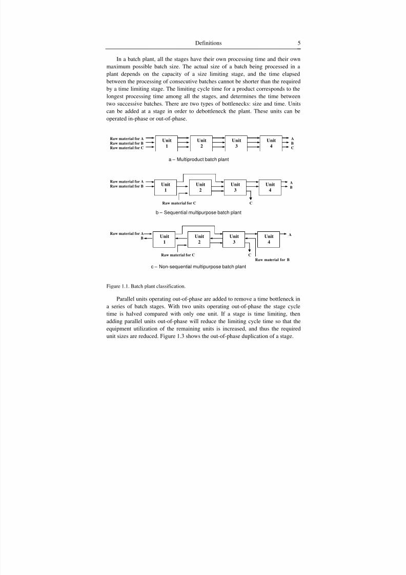
In a multiproduct plant, two or more products are produced following the
same production path. When the products are produced through different
production paths the plant is a multipurpose plant. Voudouris and Grossmann
(1996) introduced a special classification for the multipurpose batch plant. More
specifically they divided the multipurpose plants in sequential plants and non-
sequential plants (Figure 1.1). In a sequential plant it is possible to recognize a
specific direction in the plant floor that is followed by the production paths of all
the products. Non-sequential plants are all the remaining cases. Multiproduct
plants are used when the production recipes are similar to each other. As the
similarities decrease, the plant becomes a multipurpose batch plant. Among these,
sequential multipurpose plants are common in industry and hence of practical
importance.
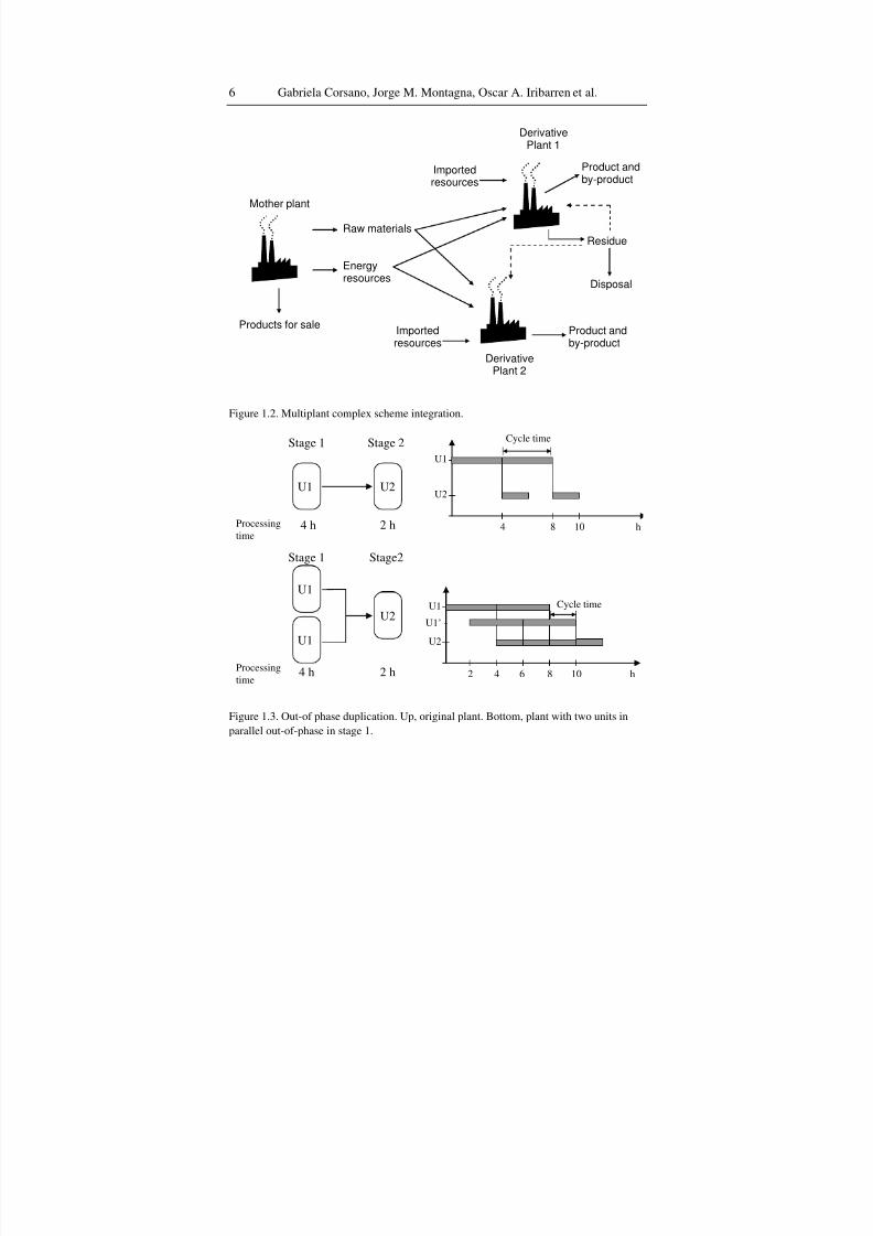
When two or more plants are nearly located and there are interconnections
between them, the integration scenario is called multiplant complex (MC)
integration. The model for a MC frequently considers mass and utility balances
between the plants, besides the design, operation, scheduling and planningconsiderations. In some cases, there is a so called “mother plant”, that supplies
raw materials and energy to others plants, called “derivative plants”. Figure 1.2
shows a MC scenario, with a mother plant and two derivative plants.
An important characteristic of batch processes is the way in which the batches
are transferred from one unit to the following one in the production path. In this
work, the Zero-wait (ZW) transfer policy is adopted. In the ZW policy the
material at any stage will be transferred immediately to the next stage after
finishing its processing. In this case, special timing constraints are required in the
model. The ZW transfer is commonly used when no intermediate storage is
available or when it cannot be held further inside the processing vessel (e.g., dueto chemical reaction). The option when storage tanks with finite capacity are
available is the finite intermediate storage (FIS) policy. When the material is
allowed to hold inside the vessel, the policy is known as non-intermediate storage
(NIS) policy.
8/7/2019 Corsano G. Montagna J.M. Iribarren O.A. Aguirre P.A. Mathematical Modeling Approaches for Optimization of Chemic…
http://slidepdf.com/reader/full/corsano-g-montagna-jm-iribarren-oa-aguirre-pa-mathematical-modeling 17/103
Definitions 5
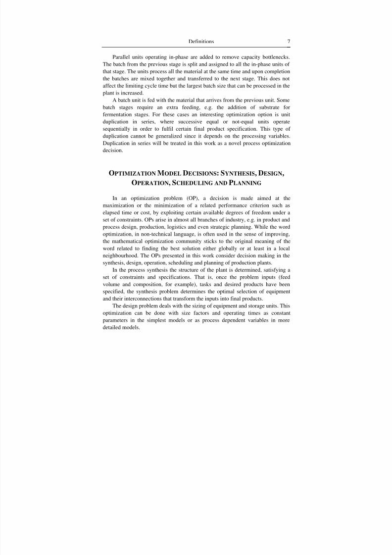
In a batch plant, all the stages have their own processing time and their own
maximum possible batch size. The actual size of a batch being processed in a
plant depends on the capacity of a size limiting stage, and the time elapsedbetween the processing of consecutive batches cannot be shorter than the required
by a time limiting stage. The limiting cycle time for a product corresponds to the
longest processing time among all the stages, and determines the time between
two successive batches. There are two types of bottlenecks: size and time. Units
can be added at a stage in order to debottleneck the plant. These units can be
operated in-phase or out-of-phase.
Unit1
Raw material for ARaw material for BRaw material for C
ABC
Unit2
Unit3
Unit4
a – Multiproduct batch plant
Unit1
Raw material for ARaw material for B
AB
Unit2
Unit3
Unit4
Raw material for C C
b – Sequential multipurpose batch plant
Unit1
Raw material for AB
AUnit2
Unit3
Unit4
Raw material for C CRaw material for B
c – Non-sequential multipurpose batch plant
Figure 1.1. Batch plant classification.
Parallel units operating out-of-phase are added to remove a time bottleneck ina series of batch stages. With two units operating out-of-phase the stage cycle
time is halved compared with only one unit. If a stage is time limiting, then
adding parallel units out-of-phase will reduce the limiting cycle time so that the
equipment utilization of the remaining units is increased, and thus the required
unit sizes are reduced. Figure 1.3 shows the out-of-phase duplication of a stage.
8/7/2019 Corsano G. Montagna J.M. Iribarren O.A. Aguirre P.A. Mathematical Modeling Approaches for Optimization of Chemic…
http://slidepdf.com/reader/full/corsano-g-montagna-jm-iribarren-oa-aguirre-pa-mathematical-modeling 18/103
Gabriela Corsano, Jorge M. Montagna, Oscar A. Iribarren et al.6
Mother plant
DerivativePlant 1
DerivativePlant 2
Products for sale
Raw materials
Energyresources
Residue
Disposal
Importedresources
Importedresources
Product andby-product
Product andby-product
Figure 1.2. Multiplant complex scheme integration.
4 h 2 h
U1 U2
U1
U2
4 8 h10
Stage 1 Stage 2
Processing
time
2 h
U1
U2
U1
4 h
U1
U2
4 8 h2 6 10Processing
time
Stage 1 Stage2
U1’
Cycle time
Cycle time
Figure 1.3. Out-of phase duplication. Up, original plant. Bottom, plant with two units in
parallel out-of-phase in stage 1.
8/7/2019 Corsano G. Montagna J.M. Iribarren O.A. Aguirre P.A. Mathematical Modeling Approaches for Optimization of Chemic…
http://slidepdf.com/reader/full/corsano-g-montagna-jm-iribarren-oa-aguirre-pa-mathematical-modeling 19/103
Definitions 7
Parallel units operating in-phase are added to remove capacity bottlenecks.
The batch from the previous stage is split and assigned to all the in-phase units of
that stage. The units process all the material at the same time and upon completionthe batches are mixed together and transferred to the next stage. This does not
affect the limiting cycle time but the largest batch size that can be processed in the
plant is increased.
A batch unit is fed with the material that arrives from the previous unit. Some
batch stages require an extra feeding, e.g. the addition of substrate for
fermentation stages. For these cases an interesting optimization option is unit
duplication in series, where successive equal or not-equal units operate
sequentially in order to fulfil certain final product specification. This type of
duplication cannot be generalized since it depends on the processing variables.
Duplication in series will be treated in this work as a novel process optimizationdecision.
OPTIMIZATION MODEL DECISIONS: SYNTHESIS, DESIGN, OPERATION, SCHEDULING AND PLANNING
In an optimization problem (OP), a decision is made aimed at the
maximization or the minimization of a related performance criterion such as
elapsed time or cost, by exploiting certain available degrees of freedom under a
set of constraints. OPs arise in almost all branches of industry, e.g. in product andprocess design, production, logistics and even strategic planning. While the word
optimization, in non-technical language, is often used in the sense of improving,
the mathematical optimization community sticks to the original meaning of the
word related to finding the best solution either globally or at least in a local
neighbourhood. The OPs presented in this work consider decision making in the
synthesis, design, operation, scheduling and planning of production plants.
In the process synthesis the structure of the plant is determined, satisfying a
set of constraints and specifications. That is, once the problem inputs (feed
volume and composition, for example), tasks and desired products have been
specified, the synthesis problem determines the optimal selection of equipmentand their interconnections that transform the inputs into final products.
The design problem deals with the sizing of equipment and storage units. This
optimization can be done with size factors and operating times as constant
parameters in the simplest models or as process dependent variables in more
detailed models.
8/7/2019 Corsano G. Montagna J.M. Iribarren O.A. Aguirre P.A. Mathematical Modeling Approaches for Optimization of Chemic…
http://slidepdf.com/reader/full/corsano-g-montagna-jm-iribarren-oa-aguirre-pa-mathematical-modeling 20/103
Gabriela Corsano, Jorge M. Montagna, Oscar A. Iribarren et al.8
The operation decisions deal with finding the optimal value for process
variables as operating times, batch sizes, concentrations, yields, etc. In the
simplest models these decision variables are involved in linear equations oralgebraic models that describe the units performance (Salomone and Iribarren,
1992). In more detailed models, this kind of decisions is described through
differential equations (Bhatia and Biegler, 1996; Corsano, et al., 2004).
Production planning determines the optimal allocation of resources within the
production facility over a time horizon of a few weeks up to a few months,
whereas short-term scheduling provides the feasible production schedules to the
plant for day to day operations. Since the boundaries of planning and scheduling
problems are not well established and there is an intrinsic integration between
these decision making stages, there is a lot of work in the literature addressing the
simultaneous consideration of planning and scheduling decisions (Wu andIerapetritou, 2007).
In multiproduct and multipurpose plant, where two or more products are
handled, an important decision to be modelled is the sequence or order in which
the products are produced. In single product campaign models all the batches of a
product are processed without overlapping with others products. On the other
hand, for mixed product campaign models a production sequence has to be
determined and the campaign is repeated over the horizon time. From the point of
view of the mathematical model, mixed product campaigns raise greater
challenges than the formulations for single product campaigns.
Table 1.1 lists the most important synthesis, design, operating and
scheduling/planning decisions and the related objective functions in order to have
a brief overview of the model complexity and characteristics.
MATHEMATICAL FORMULATIONS
Mathematical models for optimization usually lead to structured problems
such as:
• linear programming (LP) problems,• mixed integer linear programming (MILP) problems,
• nonlinear programming (NLP) problems, and
• mixed integer nonlinear programming (MINLP) problems.

8/7/2019 Corsano G. Montagna J.M. Iribarren O.A. Aguirre P.A. Mathematical Modeling Approaches for Optimization of Chemic…
http://slidepdf.com/reader/full/corsano-g-montagna-jm-iribarren-oa-aguirre-pa-mathematical-modeling 21/103
Definitions 9
Table 1.1. Problem decisions and objectives
Synthesis and Design Operation Scheduling/Planning
Decisions Plant configuration
Resources utilization
Number of units in series
Blend and recycle allocation
Unit sizes
In parallel units duplication
Intermediate storage tank
allocation
Heating and cooling areas
Power consumption (vapor
and electricity)
Batch blending, batch
splitting and batch
recycling flow rates
Material and energy
resources allocation
Component
concentrations
Unit processing times
Cycle time of each
production process
Units cycle time
Units idle time
Number of batches
Mixed campaign
configuration
Production
Objectives Minimizing the investment
cost
Minimizing the operative
costMinimizing the utilities
costs
Minimizing the
makespanMaximizing the profit
Minimizing the
inventory cost
When the objective function and constraints of the model are linear and the
optimization variables are continuous, then the problem is a LP formulation.
If some decision variables are integer, and the model has linear objective
function and constraints, then the problem is a MILP formulation.
If the objective function or some constraints are non-linear functions, and the
decision variables are continuous, then the problem is a NLP formulation. Finally,
if in the last case some variables are integer, the model is formulated through a
MINLP programming.
LITERATURE REVIEW
Since the 70s decade, many authors have contributed with new algorithms
and formulations for the mathematical modeling of diverse process optimisation
decisions. In general each one focused on a different problem, context or
structural alternative in such a way that almost all the relevant alternative
structures and options in the batch processes design and operation problems can
be considered. However, this progress has occurred as extensions of individualworks and not as complete reformulations in the sense of including all the
possibilities or at least a significant set of alternatives and decisions. There are no
models or formulations in the literature that permit consider and select among all
the possible structures and alternatives simultaneously. This is so due to the great
effort that the simultaneous resolution of the problems involves. However, in this
8/7/2019 Corsano G. Montagna J.M. Iribarren O.A. Aguirre P.A. Mathematical Modeling Approaches for Optimization of Chemic…
http://slidepdf.com/reader/full/corsano-g-montagna-jm-iribarren-oa-aguirre-pa-mathematical-modeling 22/103
Gabriela Corsano, Jorge M. Montagna, Oscar A. Iribarren et al.10
way, the trade-offs among decisions cannot be assessed. Following, the main
references about mathematical modeling in batch processes optimization are cited.
There is abundant literature on batch process synthesis and design. Themodels range from the simplest formulations as “fixed time and size factors”
(Knopf et al., 1982; Yeh and Reklaitis, 1987; Ravemark and Rippin, 1998;
Montagna et al., 2000) to the more complex as dynamic models (Bhatia and
Biegler, 1996; Corsano et al., 2004, 2006a).
The process performance models are additional algebraic equations
describing the time and size factors as functions of the units’ process variables. A
more detailed description of the performance of batch stages requires that they be
modelled with differential equations. First Barrera and Evans (1989) and later
Salomone et al. (1994) proposed that this simultaneous optimization should be
approached by integrating the batch plant model with dynamic simulationmodules for the batch units. Another way of incorporating the units’ dynamic
models is to discretize the differential equations to convert them into algebraic
constraints of the program. This was the approach used by Bhatia and Biegler
(1996) for simple process examples, and by Corsano et al. (2004, 2006) for
detailed integrated processes.
Several authors have incorporated scheduling constraints into the synthesis
problem of multiproduct and multipurpose batch plants. Again, the simplest
models are those that take fixed time and size factors (Birewar and Grossmann,
1989) which are expressed through NLP when structured decision are not
considered and MINLP otherwise. More detailed formulations where nonlinear
task models (processing time, utility usage, unit availability) and nonlinear capital
cost functions are considered, a nonconvex MINLP problem will arise (Zhang and
Sargent, 1994, 1996). Therefore, the model is very large in size and difficult to
solve. In these cases, decomposition approaches are used in order to find “good
solutions” (Barbosa-Povoa and Pantelides, 1999).
Whereas significant development has been made in the design, planning, and
scheduling of batch plants with single or multiple production routes, the problem
of synthesis, design, and operation in batch multiplant complexes has received
much less attention. Previous works have been focused on specific decision
levels. Tools and models that solve separately the different aspects of a process
have been developed. However, to obtain a good preliminary design of a
production process, it is important to consider design, synthesis, operation, and
scheduling simultaneously. There are few works in the literature dealing with
multiplant complex integration (Lee et al., 2000, Kallrath, 2002, Jackson and
Grossmann, 2003).

8/7/2019 Corsano G. Montagna J.M. Iribarren O.A. Aguirre P.A. Mathematical Modeling Approaches for Optimization of Chemic…
http://slidepdf.com/reader/full/corsano-g-montagna-jm-iribarren-oa-aguirre-pa-mathematical-modeling 23/103
Definitions 11
WORK OUTLINE
In the following sections, three problems are presented, emphasizing thedetailed mathematical formulation and results analysis in each case. In Section 2 a
superstructure optimization model is presented, that solves the synthesis, design
and operation problem for batch plants through a NLP formulation. In Section 3 a
heuristic method is presented for finding the optimal mixed product campaign
configuration of multiproduct/multipurpose batch plants. The planning problem is
simultaneously solved with the design and operation problem. The third problem
deals with the optimal processes integration in a multiplant complex. Different
aspects of design, operation, scheduling and planning are analyzed according to
diverse operational conditions and environmental issues. MC scenario solutions
are compared with multiproduct scenario solutions for a specific industrial studiedcase. Finally, a summary of the contributions of this work are outlined.

8/7/2019 Corsano G. Montagna J.M. Iribarren O.A. Aguirre P.A. Mathematical Modeling Approaches for Optimization of Chemic…
http://slidepdf.com/reader/full/corsano-g-montagna-jm-iribarren-oa-aguirre-pa-mathematical-modeling 24/103
8/7/2019 Corsano G. Montagna J.M. Iribarren O.A. Aguirre P.A. Mathematical Modeling Approaches for Optimization of Chemic…
http://slidepdf.com/reader/full/corsano-g-montagna-jm-iribarren-oa-aguirre-pa-mathematical-modeling 25/103
Chapter 3
NLP SUPERSTRUCTURE MODELING FOR THE
OPTIMAL SYNTHESIS, DESIGN AND
OPERATION IN A BATCH PLANT
3.1. INTRODUCTION
The synthesis and design problem of a batch process plant determines the
plant structure, the number of units to be used at each stage and the unit sizes.
Previously published works on this area resorted to Mixed Integer Non-Linear
models (MINLP) to solve these problems. Binary variables allowed
contemplating the allocation of units and the different alternatives to organize
them at each stage. The various models were characterized by a certain number of operations, which are the necessary steps to elaborate the product according to the
previously settled recipe. This problem was initially modelled with this format by
Grossmann and Sargent (1979).
All previous works on this area start from a plant where the number of stages
is settled by a decision made in a previous step, taking into account that synthesis
and design problems are separately solved. Thus, the only structural decision that
usually remains is the one related to unit duplication at each previously
determined stage. However, there are many operations that pose alternatives as
regards the number of stages to be used that cannot be considered with this
approach. For example in the case of fermentation, depending on reaction rate,equipment cost, or raw material availability, the number of units to be used and
the way in which they should operate (in series or in parallel) may vary. Then
these options should be considered in relation to the sizing decisions. As
illustrated with this example, a strong relationship exists among the number of
stages, the way in which each stage is configured and the operative characteristics
8/7/2019 Corsano G. Montagna J.M. Iribarren O.A. Aguirre P.A. Mathematical Modeling Approaches for Optimization of Chemic…
http://slidepdf.com/reader/full/corsano-g-montagna-jm-iribarren-oa-aguirre-pa-mathematical-modeling 26/103
Gabriela Corsano, Jorge M. Montagna, Oscar A. Iribarren et al.14
of stages (fermentors feeding, processing times, substrate concentration, among
others), which has not been posed yet. This is due to the difficulties in solving a
problem in which all these elements are optimization variables.This work intends to solve the aforementioned problem. Firstly, a model with
a high level of detail is posed. Operations have been represented through
discretized differential equations that describe mass balances. Furthermore,
constraints on feeds to each processing unit and equations of interconnections
between stages are considered. This level of detail has been posed by few authors.
Some exceptions that can be mentioned are Bhatia and Biegler (1996), even
though with a simpler model since they work with a predetermined number of
stages and they do not admit units duplication.
The option of optimizing the number of stages in series to be considered in
this work has not been included in previous general models of batch plants design.The plant structure problems have been solved in previous synthesis models
resorting to binary variables. It should be stressed that in many cases, when the
level of detail of the operations included in the process was significant (Bhatia
and Bieglier, 1996; Barrrera and Evans, 1989) this last option was not even
considered. As previously pointed, this formulation leads to difficulties or limits
the capacity for solving the model.
This work optimizes the plant superstructure in order to model this problem.
This is a systematic method for the synthesis of chemical process networks. For
the given raw materials and final products, there are a lot of feasible production
paths that can produce the desired products. In a superstructure optimization
model, all the possible alternatives for the process are included in the overall
model. In order to obtain the optimal solution, the resolution procedure selects the
optimal production alternative among the available options.
This work proposes to explicitly include a superstructure that contemplates all
possible options for the plant structure with units in series or in parallel. These
alternatives can be obtained by means of different mechanisms. Corsano et al.
(2004) presented a heuristic procedure through a simplified optimization model
that provides an upper bound for the number of stages of each operation. Another
option is to pose an exhaustive enumeration of all the alternatives that arise from
the upper bounds for the units in series or in parallel. The designer’s criteria and
his or her experience are also critical to bound the superstructure size by taking
into account only the most expensive units with a significant impact on the
process performance.
An original approach is developed to solve the model where discrete
alternatives are selected without resorting to binary variables. Taking into account
that the model is a non-convex NLP due to the equations that describe the plant
8/7/2019 Corsano G. Montagna J.M. Iribarren O.A. Aguirre P.A. Mathematical Modeling Approaches for Optimization of Chemic…
http://slidepdf.com/reader/full/corsano-g-montagna-jm-iribarren-oa-aguirre-pa-mathematical-modeling 27/103
NLP Superstructure Modeling for the Optimal Synthesis… 15
operations, difficulties of resolution methodologies for MINLP programs are
avoided. This kind of models is usually solved through methods like the outer
approximation algorithm (Duran and Grossmann, 1986; Viswanathan andGrossmann, 1990; Varvarezos et al., 1992) where a sequence of NLP and MILP
problems is solved. The available MINLP algorithms can miss the optimal
solution due to the application of linear cuts to non-convex regions. On the other
hand, our optimisation approach finds the optimal solution by modeling a
superstructure with as options as proposed by the designer. The optimal solution
will eventually eliminate units of the network taking their size to be zero. In this
way we solve the model as a NLP problem instead of a MINLP problem. With
this approach, the user can provide physically meaningful initializations
increasing the robustness and usefulness of the optimization models. Available
computer codes for solving MINLP are of general purpose and do not use initialsolutions as those proposed in this work. Finally, the major advantage of this
strategy is that all the alternatives can be explored explicitly because their number
is relatively low. Therefore, the work presents a problem representation which is
extremely compact and allows for taking into consideration a significant number
of alternatives.
The developed model is presented working on the case of a fermentors
network. It is a typical case for a number of reasons. First of all, it is often present
in agro-industrial and biotechnological plants. In addition, it is necessary to
represent the process with a high level of detail, due to its high economic impact
on the plant cost. Taking into account the operation characteristics, it is required
to duplicate stages both in series and in parallel. On the other hand, the number of
options to be contemplated is bounded by operative considerations. It is important
to mention that this approach could be easily extended to other kind of reactions.
In the next section, a general model for a single product plant is presented. The
model can be easily extended to the multiproduct case where many products are
made with the same equipment. Then, its application to the case of a fermentors
network is described. The resolution of this example allows assessing the
potentiality of the proposed approach. Finally, it is compared to a traditional
formulation in which the structural decisions of the plant are represented by
means of binary variables.
3.2. MODEL FORMULATION
We consider a plant that produces only one product and must meet a certain
demand Q for that product on the available time horizon H .
8/7/2019 Corsano G. Montagna J.M. Iribarren O.A. Aguirre P.A. Mathematical Modeling Approaches for Optimization of Chemic…
http://slidepdf.com/reader/full/corsano-g-montagna-jm-iribarren-oa-aguirre-pa-mathematical-modeling 28/103
Gabriela Corsano, Jorge M. Montagna, Oscar A. Iribarren et al.16
To complete the product processing, P operations are required. Each
operation is accomplished over several stages j, whose optimal number has to be
determined. For each operation p, there is an upper bound C p on the number of stages to be contemplated for this operation. In this way, the number of stages to
be considered for each operation can be modified. Therefore, for each operation p,
there is a set of stages j ranging from 1 to C p, whose utilization must be
determined as a solution to the optimization problem.
It should be pointed that this approach is more realistic when the operation of
each stage can be represented by means of a detailed model and is not fixed by a
size factor as in the first examples referred to in the introduction section. In this
way, it is possible to take into account the different tradeoffs that arise when
considering different operative conditions. Therefore, the model to solve the batch
operations design becomes more appropriate when the description of the stagesoperation is explicitly contemplated.
For each operation p, alternatives a = 1, ..., Ap are defined. These alternatives
can be either automatically generated (through an optimization model, for
example) or proposed by the designer, which is more effective taking into account
the feasible options for the kind of process they are working with. Each existing
alternative a in operation p must be characterized. This implies defining the
following elements:
• Number of stages to be included in the alternative.
• Determining the last stage being included in the alternative (basic informationto allow for connection between successive operations).
• Number of in-phase (Gpaj) and out-of-phase (M paj) duplicated units for each
stage included in the alternative.
The existing j stages in alternative a of operation p may vary between 1 and
C p. For each alternative, the number of stages is predetermined. Each one of these
alternatives has structural options due to the duplication of the units included in it.
These options are predetermined in each alternative a.
The transfer policy considered in this work is the Zero Wait (ZW) transfer. A
stage-configuration option is in series duplication. In this case, the cycle time
(problem variable) for a plant is determined as the longest time of all the stages
over each operation involved in the production process. This cycle time settles
down the time between two successive batches. Therefore, all the units that
require less operating time have some idle time. Aiming at reducing this time, out-
of-phase parallel units can be included into the stage in which the cycle time is
reached. These units operate out-of-phase, thus allowing for reducing the time
8/7/2019 Corsano G. Montagna J.M. Iribarren O.A. Aguirre P.A. Mathematical Modeling Approaches for Optimization of Chemic…
http://slidepdf.com/reader/full/corsano-g-montagna-jm-iribarren-oa-aguirre-pa-mathematical-modeling 29/103
NLP Superstructure Modeling for the Optimal Synthesis… 17
spent between two successive batches, and consequently the remaining units size
is reduced as a result of having less idle time.
The other configuration option for units duplication is in-phase, in whichduplicated units operate simultaneously. In this case, when the batch enters that
stage, it is split among all units belonging to the stage, and when finishing the
operation the exiting batches are added together. In this way, the processing
capacity of a stage can be increased, which is important when the unit size reaches
the upper bound.
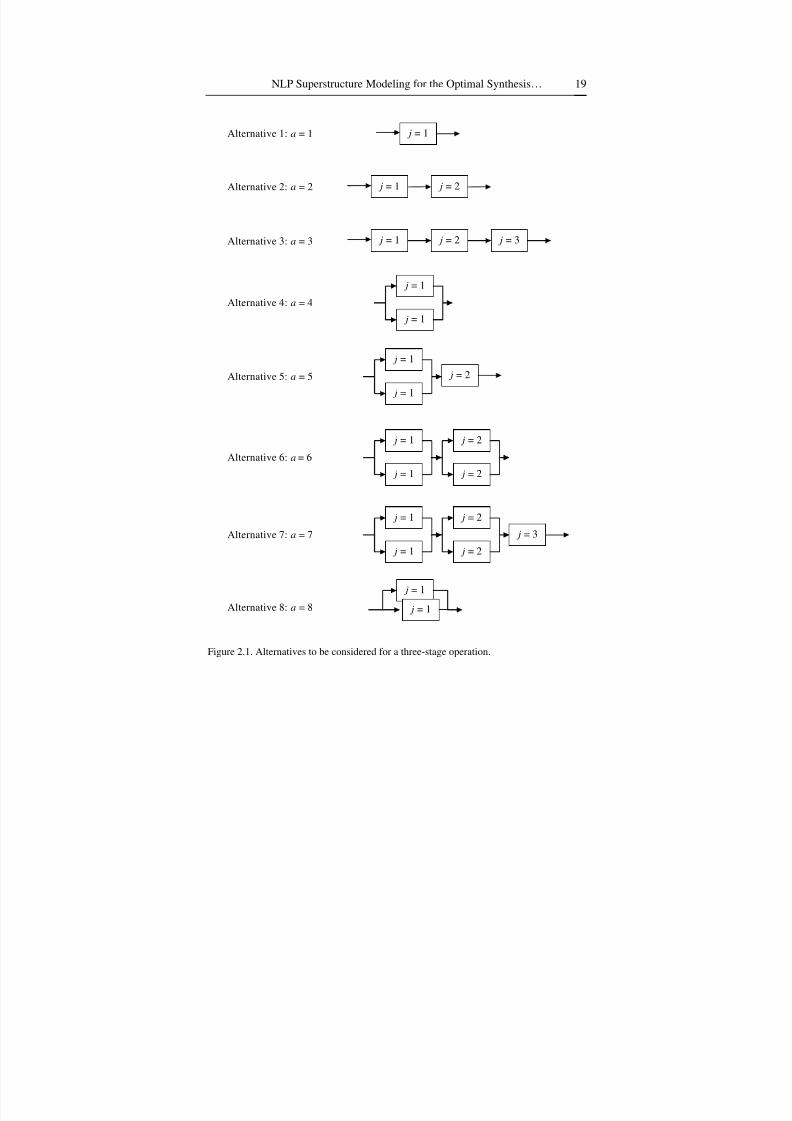
Figure 2.1 shows an example. An operation (P = 1) has C p = 3 stages, which
indicates that any alternative being used in this operation can have at most 3
stages. The problem designer has settled that the A= 8 alternatives shown in
Figure 2.1 should be taken into account. The j stages used in the corresponding a
alternative are also indicated. The first alternative includes only one stage,whereas the following two have additional stages in series. The other alternatives
included out-of-phase duplicated units for various stages, except for the last one
(a= 8), which is the only stage in which in-phase duplicated units are considered.
This is shown through overlapped units in Figure 2.1.
The model looks for a plant design that allows producing the required
quantity Q in time horizon H at the lowest cost. This general presentation takes
into account unit costs and operative costs. The objective function is Total Annual
Cost (TAC ) minimization and is calculated from the following expression:
pa
p
1 1 j
p
p
p p
AP
paj paj paj
p a a
Min M G V OC β α = = ∈
+∑ ∑ ∑ (2.1)
V paj is unit j size in alternative a for operation p. Its cost is calculated from
coefficients αp and βp that are usually used in this kind of problems (Ravemark
and Rippin, 1998). M paj and Gpaj correspond to the number of out-of-phase and in-
phase duplicated units, respectively, for stage j in alternative a for operation p and
they are provided by the designer. OC represents operating costs that depend on
how each operation is performed and thus it cannot be represented through a
general expression.In the previous expression, all stages j of all existing alternatives for operation
p are considered. Taking into account that the objective function minimizes the
units cost, only the best structural option will be chosen, driving to zero the size of
all units that are not involved in the optimal structure. The simultaneous operation
of two structures will always involve a greater cost taking into account that the
8/7/2019 Corsano G. Montagna J.M. Iribarren O.A. Aguirre P.A. Mathematical Modeling Approaches for Optimization of Chemic…
http://slidepdf.com/reader/full/corsano-g-montagna-jm-iribarren-oa-aguirre-pa-mathematical-modeling 30/103
Gabriela Corsano, Jorge M. Montagna, Oscar A. Iribarren et al.18
exponent coefficient βp is less than one. For that reason, the unit sizes of non-
optimal alternatives will be equal to zero.
According to this problem formulation, a set of constraints are developed.First of all, the required demand Q should be satisfied. For that purpose, the plant
production rate PR is employed, which is given by:
QPR
H = (2.2)
At the last stage of the last operation, the final product is obtained. The sum
of the productions of all the defined alternatives must meet the production
requirement for the plant:
,last la st
last
p aj
a p
PR PR∈
≥∑ (2.3)
where plast corresponds to the last operation of the process and jlast to the last stage
in each option a. Therefore, ,last p aPR represents the production rate achieved at
each alternative a in the last operation.
The total amount produced should be at least equal to the plant requirement.
Since the model tries to minimize costs, the quantity to be produced will be just
PR, and will be reached by using only one alternative in operation plast . This willbe so because in case of using two alternatives it will be necessary to use
equipment for both of them, which would notably increase the cost.
It is required to determine the plant cycle time TL. This is determined by the
longest time required in the stages being used at the plant. Let T paj be the unit
operation time at stage j for alternative a in operation p. This value is calculated
from the model that describes that operation. Then, considering ZW policy, it
should be:
paj
paj
T TL
M
≥ 1, ..., , 1, ..., , 1, ...,p p
p P a A j C ∀ = = = (2.4)
M paj corresponds to the number of out-of-phase duplicated units that exist at
stage j of alternative a in operation p.
8/7/2019 Corsano G. Montagna J.M. Iribarren O.A. Aguirre P.A. Mathematical Modeling Approaches for Optimization of Chemic…
http://slidepdf.com/reader/full/corsano-g-montagna-jm-iribarren-oa-aguirre-pa-mathematical-modeling 31/103
NLP Superstructure Modeling for the Optimal Synthesis… 19
Alternative 1: a = 1 j = 1
j = 1 j = 2Alternative 2: a = 2
j = 3j = 1 j = 2Alternative 3: a = 3
Alternative 4: a = 4
Alternative 5: a = 5
j = 1
j = 1
j = 2
Alternative 6: a = 6j = 2
j = 2
j = 1
j = 1
j = 1
j = 1
Alternative 7: a = 7
j = 2
j = 2
j = 1
j = 1
j = 3
Alternative 8: a = 8
j = 1
j = 1
Figure 2.1. Alternatives to be considered for a three-stage operation.
8/7/2019 Corsano G. Montagna J.M. Iribarren O.A. Aguirre P.A. Mathematical Modeling Approaches for Optimization of Chemic…
http://slidepdf.com/reader/full/corsano-g-montagna-jm-iribarren-oa-aguirre-pa-mathematical-modeling 32/103
Gabriela Corsano, Jorge M. Montagna, Oscar A. Iribarren et al.20
Connection balances should be accounted for between successive stages of
each alternative of an operation. Letini
pajB and
fin
pajB be the batch volume that
enters and leaves the unit of stage j in alternative a in operation p; then the
balances are:
, 1
ini fin
paj pa jB B −= 1,..., , 1,..., , 2
P pap P a A j∀ = = ≥ (2.5)
In case of handling several material streams, this kind of connection
constraint should be settled for each of them. As will be seen in the example, this
balance can also consider adding extra feeds at each stage.
Connection between successive operations must be also assured. For that
reason, the last stage of an operation must get in contact with the first stage of thefollowing operation:
1, ,1
1
,1
last p a
p p
fin ini
pa j
a p a p
B B+
+∈ ∈ +
=∑ ∑ 1, ..., 1p P∀ = − (2.6)
In this case, the total material exiting the last stage jlast of all alternatives of
operation p, must be equal to all the material entering the first stage of all
alternatives of the following operation.
The Bpaj and T paj values being used must be characterized through appropriate
equations. Also the material streams to be considered could be decomposed into
several components (substrate, biomass, product, etc.) as it will be shown in the
following example. The existing relationship among the material to be processed,
the equipment sizes and the time that will be required for processing, arises from
the model to be used for describing the involved operation.
Therefore, there is a set of constraints that closely depend on the
characteristics of the process being used, and thus it is not possible to formalize
them with a general format.
3.3. FERMENTATION PROCESS FOR ETHANOL PRODUCTION
In this example corresponding to fermentation for ethanol production, the
previously described model is applied to a specific case. The detailed models
describing each unit operation are introduced next.
8/7/2019 Corsano G. Montagna J.M. Iribarren O.A. Aguirre P.A. Mathematical Modeling Approaches for Optimization of Chemic…
http://slidepdf.com/reader/full/corsano-g-montagna-jm-iribarren-oa-aguirre-pa-mathematical-modeling 33/103
NLP Superstructure Modeling for the Optimal Synthesis… 21
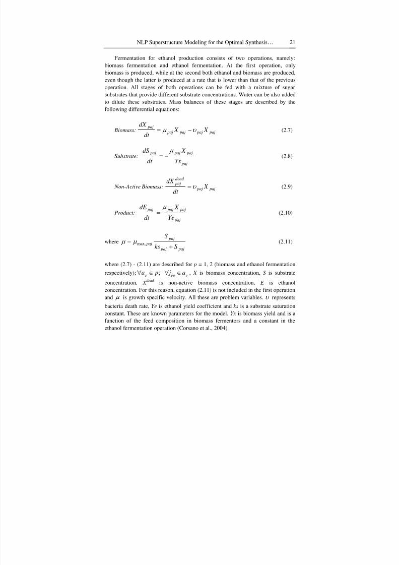
Fermentation for ethanol production consists of two operations, namely:
biomass fermentation and ethanol fermentation. At the first operation, only
biomass is produced, while at the second both ethanol and biomass are produced,even though the latter is produced at a rate that is lower than that of the previous
operation. All stages of both operations can be fed with a mixture of sugar
substrates that provide different substrate concentrations. Water can be also added
to dilute these substrates. Mass balances of these stages are described by the
following differential equations:
Biomass: pajpajpajpaj
pajX X
dt
dX υ μ −= (2.7)
Substrate: paj
pajpajpaj
Yx
X
dt
dS−= (2.8)
Non-Active Biomass: pajpaj
dead paj
X dt
dX υ = (2.9)
Product: paj
pajpajpaj
Ye
X
dt
dE = (2.10)
where
pajpaj
paj
pajSks
S
+= max,μ μ (2.11)
where (2.7) - (2.11) are described for p = 1, 2 (biomass and ethanol fermentation
respectively); ;p pa pa p j a∀ ∈ ∀ ∈ , X is biomass concentration, S is substrate
concentration, X dead is non-active biomass concentration, E is ethanol
concentration. For this reason, equation (2.11) is not included in the first operation
and is growth specific velocity. All these are problem variables. υ represents
bacteria death rate, Ye is ethanol yield coefficient and ks is a substrate saturation
constant. These are known parameters for the model. Yx is biomass yield and is a
function of the feed composition in biomass fermentors and a constant in the
ethanol fermentation operation (Corsano et al., 2004).
8/7/2019 Corsano G. Montagna J.M. Iribarren O.A. Aguirre P.A. Mathematical Modeling Approaches for Optimization of Chemic…
http://slidepdf.com/reader/full/corsano-g-montagna-jm-iribarren-oa-aguirre-pa-mathematical-modeling 34/103
Gabriela Corsano, Jorge M. Montagna, Oscar A. Iribarren et al.22
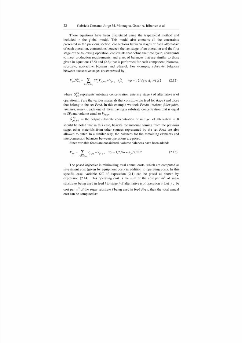
These equations have been discretized using the trapezoidal method and
included in the global model. This model also contains all the constraints
presented in the previous section: connections between stages of each alternativeof each operation, connections between the last stage of an operation and the first
stage of the following operation, constraints that define the time cycle, constraints
to meet production requirements, and a set of balances that are similar to those
given in equations (2.5) and (2.6) that is performed for each component: biomass,
substrate, non-active biomass and ethanol. For example, substrate balances
between successive stages are expressed by:
, , 1 , 1
paj
ini fin
paj paj f f paj pa j pa j
f Feed
V S SF V V S− −∈
= +∑ 1,2; ; 2p
p a A j∀ = ∀ ∈ ∀ ≥ (2.12)
whereini
pajS represents substrate concentration entering stage j of alternative a of
operation p, f are the various materials that constitute the feed for stage j and those
that belong to the set Feed . In this example we took Feed = {molass, filter juice,
vinasses, water }, each one of them having a substrate concentration that is equal
to SF f and volume equal to V f,paj.
, 1
fin
pa jS − is the output substrate concentration of unit j-1 of alternative a. It
should be noted that in this case, besides the material coming from the previous
stage, other materials from other sources represented by the set Feed are also
allowed to enter. In a similar way, the balances for the remaining elements andinterconnection balances between operations are posed.
Since variable feeds are considered, volume balances have been added:
, , 1
paj
paj f paj pa j
f Feed
V V V −∈
= +∑ 1,2; ; 2p
p a A j∀ = ∀ ∈ ∀ ≥ (2.13)
The posed objective is minimizing total annual costs, which are computed as
investment cost (given by equipment cost) in addition to operating costs. In this
specific case, variable OC of expression (2.1) can be posed as shown by
expression (2.14). This operating cost is the sum of the cost per m
3
of sugarsubstrates being used in feed f to stage j of alternative a of operation p. Let
f γ be
cost per m3 of the sugar substrate f being used in feed Feed , then the total annual
cost can be computed as:
8/7/2019 Corsano G. Montagna J.M. Iribarren O.A. Aguirre P.A. Mathematical Modeling Approaches for Optimization of Chemic…
http://slidepdf.com/reader/full/corsano-g-montagna-jm-iribarren-oa-aguirre-pa-mathematical-modeling 35/103
NLP Superstructure Modeling for the Optimal Synthesis… 23
pa pa
p ,
1 1 j 1 1 j
p p
p
p p p p
A AP P
ann paj paj paj f f paj
p a a p a a f Feed
H Min C M G V V
TL
β α γ
= = ∈ = = ∈ ∈
⎧ ⎫⎪ ⎪+⎨ ⎬
⎪ ⎪⎩ ⎭
∑ ∑ ∑ ∑ ∑ ∑ ∑ (2.14)
3.4. EXAMPLE RESOLUTION
The fermentation model for ethanol production established in the previous
section has been solved. Three examples will be presented with different sets of
data with the aim of evaluating the optimal design of the plant according to
various problem conditions.
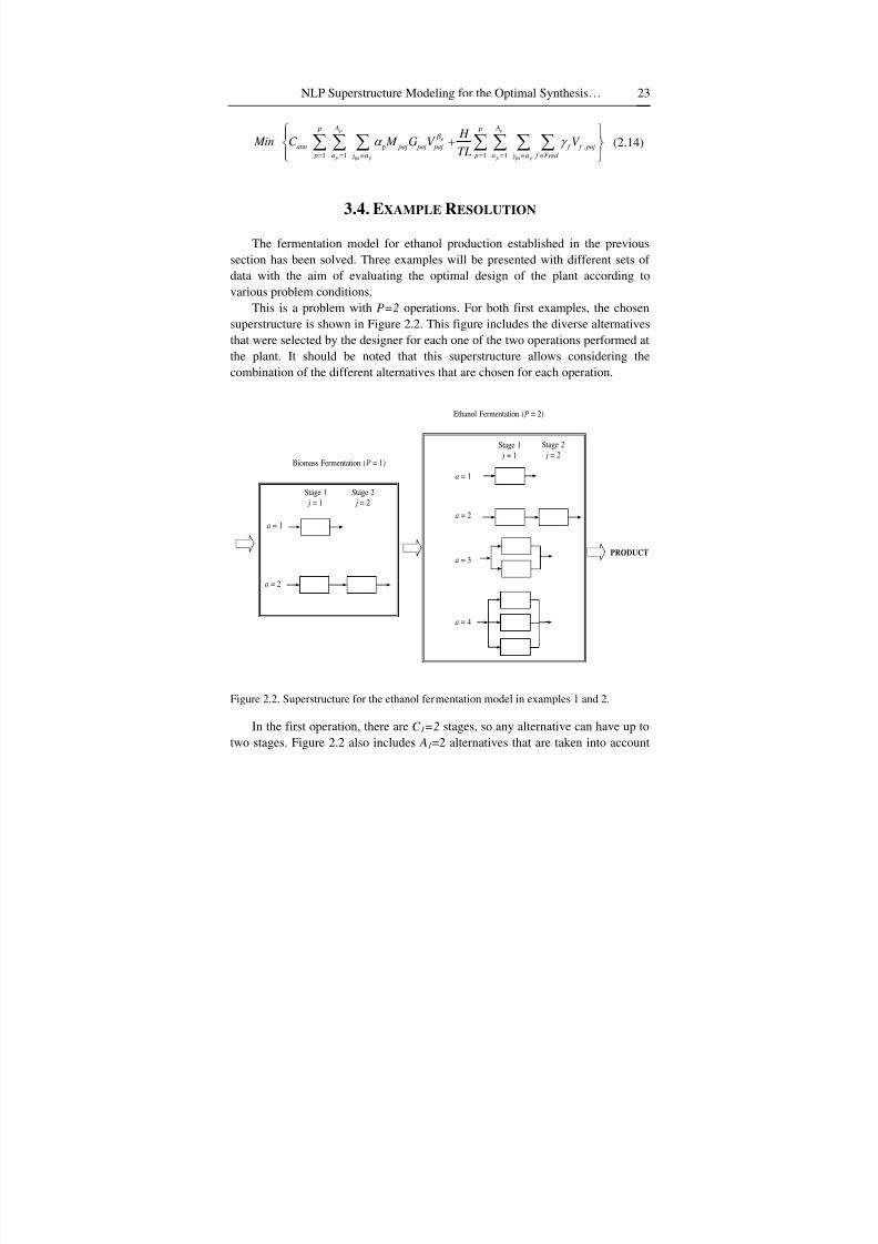
This is a problem with P=2 operations. For both first examples, the chosen
superstructure is shown in Figure 2.2. This figure includes the diverse alternativesthat were selected by the designer for each one of the two operations performed at
the plant. It should be noted that this superstructure allows considering the
combination of the different alternatives that are chosen for each operation.
Ethanol Fermentation (P = 2)
Stage 1j = 1
Stage 2j = 2
Stage 1
j = 1
Stage 2
j = 2Biomass Fermentation (P = 1)
a = 1
a = 2
a = 1
a = 2
a = 3
a = 4
PRODUCT
Figure 2.2. Superstructure for the ethanol fermentation model in examples 1 and 2.
In the first operation, there are C 1=2 stages, so any alternative can have up to
two stages. Figure 2.2 also includes A1=2 alternatives that are taken into account
8/7/2019 Corsano G. Montagna J.M. Iribarren O.A. Aguirre P.A. Mathematical Modeling Approaches for Optimization of Chemic…
http://slidepdf.com/reader/full/corsano-g-montagna-jm-iribarren-oa-aguirre-pa-mathematical-modeling 36/103
Gabriela Corsano, Jorge M. Montagna, Oscar A. Iribarren et al.24
in this operation. In the first one, there is only one stage, while in the second one
there are two stages in series. For the second operation, A2 = 4 alternatives of up to
C 2 = 2 stages are considered. In this case, the first alternative consists of only onestage, the second one consists of two stages in series, the third one is the out-of-
phase in parallel duplication of the first stage and the last one is the out-of-phase
triplication of the first stage. The selection of alternatives for these operations is
assumed to be based on the knowledge that the designer has about the problem,
regarding its feasibility from an engineering point of view. In this case, as the
reaction rate of the biomass fermentation operation is faster than that of the
ethanol fermentation operation, the processing time of the first operation is lower
than that of the second and therefore the option of in parallel stages duplication in
not included for the first operation.
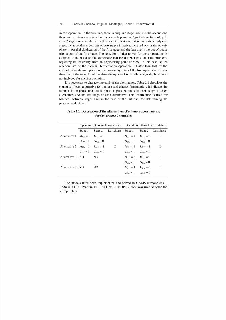
It is necessary to characterize each of the alternatives. Table 2.1 describes theelements of each alternative for biomass and ethanol fermentation. It indicates the
number of in-phase and out-of-phase duplicated units at each stage of each
alternative, and the last stage of each alternative. This information is used for
balances between stages and, in the case of the last one, for determining the
process production.
Table 2.1. Description of the alternatives of ethanol superstructurefor the proposed examples
Operation: Biomass Fermentation Operation: Ethanol FermentationStage 1 Stage 2 Last Stage Stage 1 Stage 2 Last Stage
Alternative 1 M 111 = 1
G111 = 1
M 112 = 0
G112 = 0
1 M 211 = 1
G211 = 1
M 212 = 0
G212 = 0
1
Alternative 2 M 121 = 1
G121 = 1
M 122 = 1
G122 = 1
2 M 221 = 1
G221 = 1
M 222 = 1
G222 = 1
2
Alternative 3 NO NO M 231 = 2
G231 = 1
M 232 = 0
G232 = 0
1
Alternative 4 NO NO M 241 = 3G241 = 1
M 242 = 0G242 = 0
1
The models have been implemented and solved in GAMS (Brooke et al.,
1998) in a CPU Pentium IV, 1.60 Ghz. CONOPT 2 code was used to solve the
NLP problem.
8/7/2019 Corsano G. Montagna J.M. Iribarren O.A. Aguirre P.A. Mathematical Modeling Approaches for Optimization of Chemic…
http://slidepdf.com/reader/full/corsano-g-montagna-jm-iribarren-oa-aguirre-pa-mathematical-modeling 37/103
NLP Superstructure Modeling for the Optimal Synthesis… 25
The model parameters values for the following examples are shown in Table
2.2.
Table 2.2. Parameters used in the ethanol production model
Parameter Value
aj1max, 0.5 h-1
aj2max, 0.1 h-1
pα 115550
pajυ 0.02 h-1
Yx2aj 0.124
Ye2aj 0.23
H 7500 h year-1
kspaj 20 k m-3
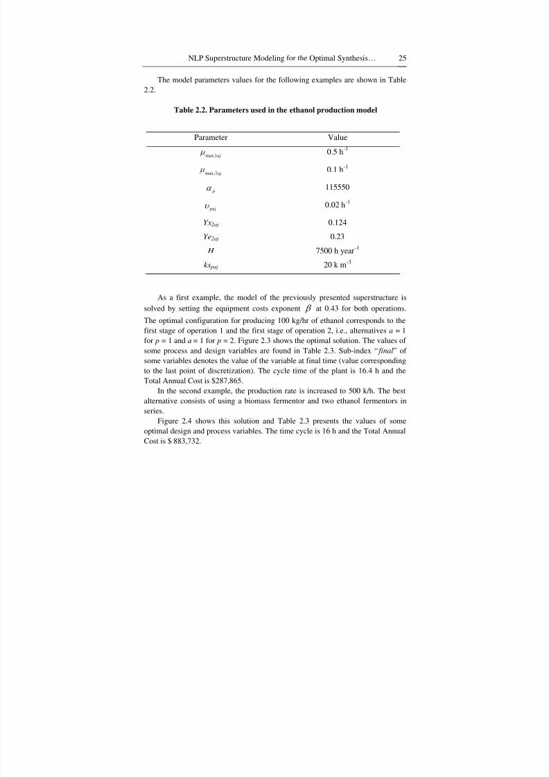
As a first example, the model of the previously presented superstructure is
solved by setting the equipment costs exponent β at 0.43 for both operations.
The optimal configuration for producing 100 kg/hr of ethanol corresponds to the
first stage of operation 1 and the first stage of operation 2, i.e., alternatives a = 1
for p = 1 and a = 1 for p = 2. Figure 2.3 shows the optimal solution. The values of
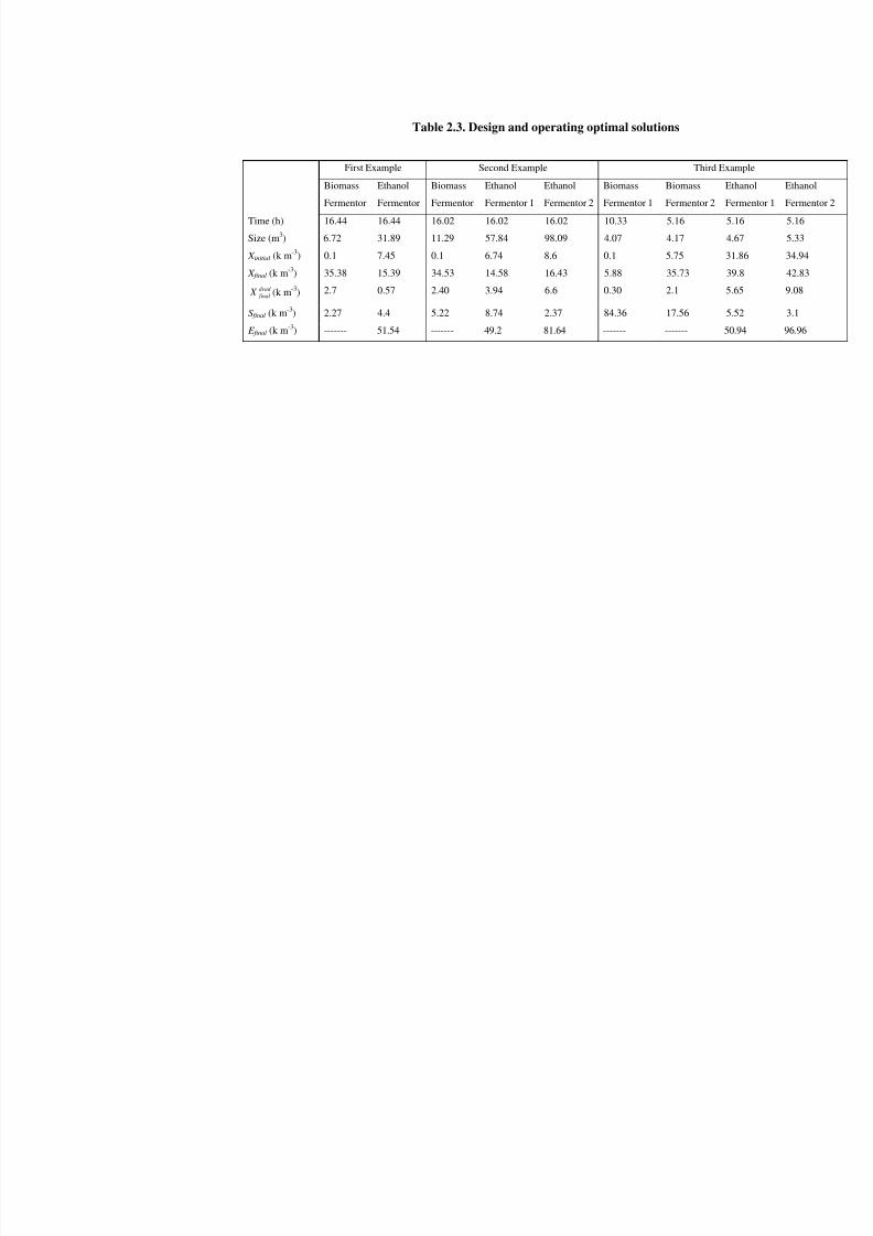
some process and design variables are found in Table 2.3. Sub-index “ final” of
some variables denotes the value of the variable at final time (value corresponding
to the last point of discretization). The cycle time of the plant is 16.4 h and the
Total Annual Cost is $287,865.
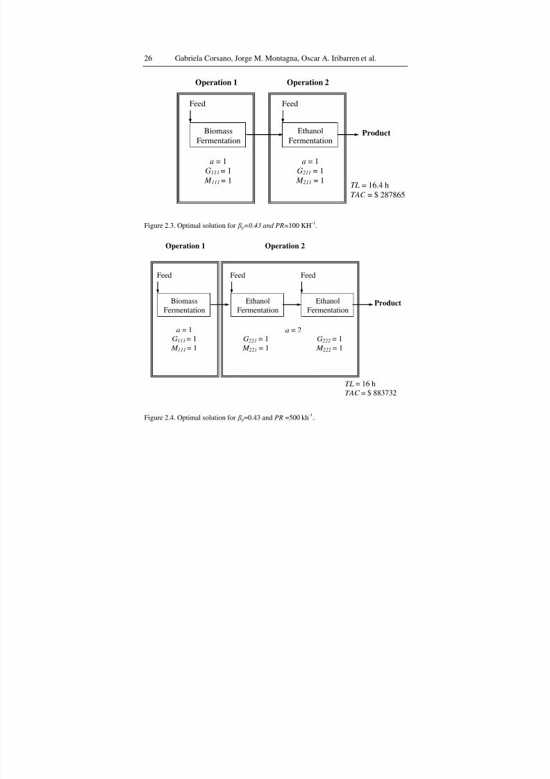
In the second example, the production rate is increased to 500 k/h. The best
alternative consists of using a biomass fermentor and two ethanol fermentors in
series.
Figure 2.4 shows this solution and Table 2.3 presents the values of some
optimal design and process variables. The time cycle is 16 h and the Total Annual
Cost is $ 883,732.
8/7/2019 Corsano G. Montagna J.M. Iribarren O.A. Aguirre P.A. Mathematical Modeling Approaches for Optimization of Chemic…
http://slidepdf.com/reader/full/corsano-g-montagna-jm-iribarren-oa-aguirre-pa-mathematical-modeling 38/103
Gabriela Corsano, Jorge M. Montagna, Oscar A. Iribarren et al.26
BiomassFermentation
EthanolFermentation
a = 1G111 = 1M 111 = 1
a = 1G211 = 1M 211 = 1
Feed Feed
Product
TL = 16.4 hTAC = $ 287865
Operation 1 Operation 2
Figure 2.3. Optimal solution for β p=0.43 and PR=100 KH-1
.
TL = 16 hTAC = $ 883732
BiomassFermentation
a = 1G111 = 1
M 111 = 1
Feed Feed
EthanolFermentation
Feed
G221 = 1
M 221 = 1
EthanolFermentation Product
G222 = 1
M 222 = 1
Operation 1 Operation 2
a = 2
Figure 2.4. Optimal solution for β p=0.43 and PR =500 kh-1
.
8/7/2019 Corsano G. Montagna J.M. Iribarren O.A. Aguirre P.A. Mathematical Modeling Approaches for Optimization of Chemic…
http://slidepdf.com/reader/full/corsano-g-montagna-jm-iribarren-oa-aguirre-pa-mathematical-modeling 39/103
Table 2.3. Design and operating optimal solutions
First Example Second Example Third Exam
Biomass
Fermentor
Ethanol
Fermentor
Biomass
Fermentor
Ethanol
Fermentor 1
Ethanol
Fermentor 2
Biomass
Fermentor 1
Biomass
Fermentor 2
Eth
Ferm
Time (h) 16.44 16.44 16.02 16.02 16.02 10.33 5.16 5.16
Size (m3) 6.72 31.89 11.29 57.84 98.09 4.07 4.17 4.67
X initial (k m-3) 0.1 7.45 0.1 6.74 8.6 0.1 5.75 31.8
X final (k m-3) 35.38 15.39 34.53 14.58 16.43 5.88 35.73 39.8
dead
finalX (k m-3) 2.7 0.57 2.40 3.94 6.6 0.30 2.1 5.65
Sfinal (k m-3) 2.27 4.4 5.22 8.74 2.37 84.36 17.56 5.52
E final (k m-3) ------- 51.54 ------- 49.2 81.64 ------- ------- 50.9
8/7/2019 Corsano G. Montagna J.M. Iribarren O.A. Aguirre P.A. Mathematical Modeling Approaches for Optimization of Chemic…
http://slidepdf.com/reader/full/corsano-g-montagna-jm-iribarren-oa-aguirre-pa-mathematical-modeling 40/103
Ethanol Fermentation (p = 2)
Stage 1j = 1
Stage 2j = 2
Stage 1j = 1
Stage 2j = 2
Biomass Fermentation (p = 1)
a = 1
a = 2
a = 1
a = 2
a = 3
a = 4
a = 3
a = 4
a = 5
a = 6
Figure 2.5. Superstructure for the ethanol fermentation model in example 3.
8/7/2019 Corsano G. Montagna J.M. Iribarren O.A. Aguirre P.A. Mathematical Modeling Approaches for Optimization of Chemic…
http://slidepdf.com/reader/full/corsano-g-montagna-jm-iribarren-oa-aguirre-pa-mathematical-modeling 41/103
NLP Superstructure Modeling for the Optimal Synthesis… 29
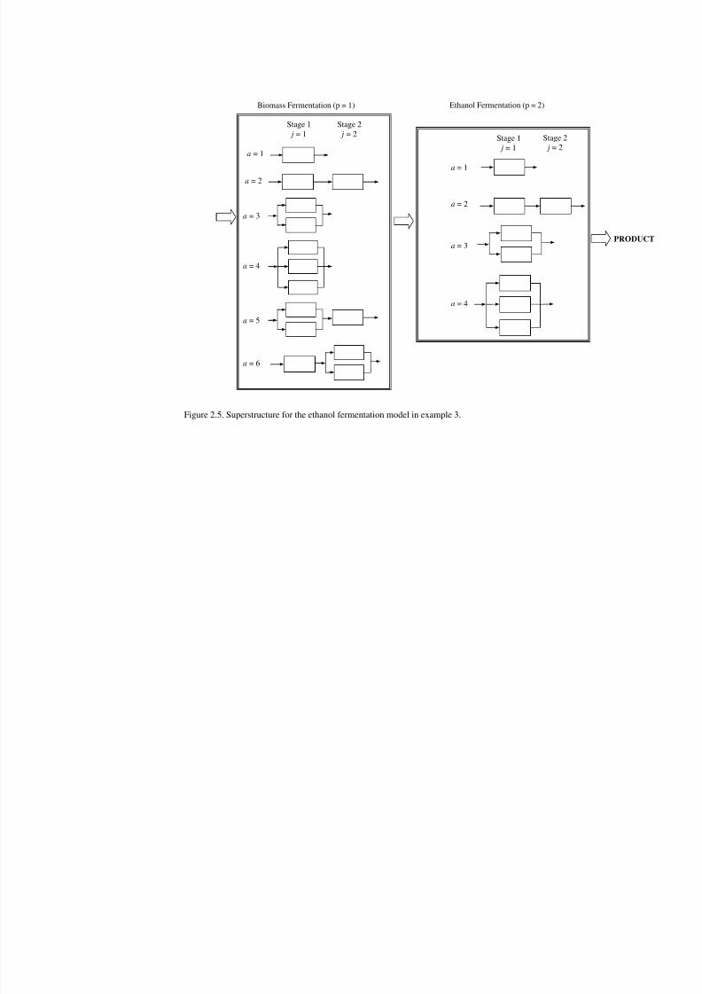
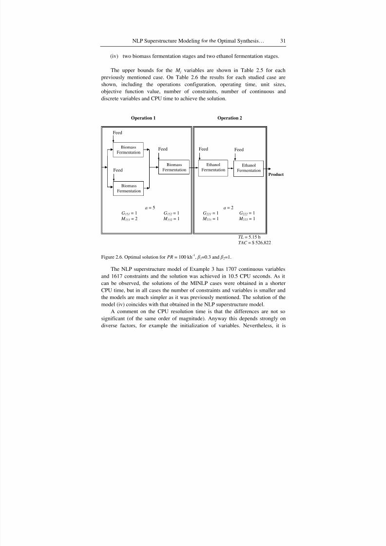
In the third example we decreased the equipment cost exponent of the first
operation ( 1β ) to 0.3 and increased the second ones ( 2β ) to 1. For this case, we
changed the superstructure presented on Table 2.1. Table 2.4 shows the
information about the superstructure for both biomass and ethanol fermentation
operation, and Figure 2.5 shows this superstructure. The optimal solution consists
of the out-of-phase in parallel duplication of the first biomass fermentor followed
by one biomass fermentor and two ethanol fermentors in series. This solution
corresponds to Alternative 5 of the first operation and Alternative 2 of the second
one. Figure 2.6 shows this solution and Table 2.3 presents some of its optimal
variables. In-parallel working equipment has the same operative and design
characteristics (operation time, size, feeds, flows, etc.). The time cycle is 5.15 h
and the Total Annual Cost is $526,822.
3.5. A COMPARISON WITH THE TRADITIONAL APPROACH
A comparison will be made between the proposed approach, in which the
different alternatives of the plant configuration are modelled without resorting to
binary variables, and the traditional approach, in which the problem is represented
through a MINLP program.
Firstly, it should be highlighted that traditional models do not solve this
problem by considering in series stages duplication. Consequently, in order to
perform a comparison, we assume that the number of plant stages is fixed, and
thus we are facing a problem that is sensibly simpler than the one presented in this
work. Therefore, the only way of comparing both approaches is solving a
sequence of MINLP problems that contemplate all the alternatives. This could be
made in this example because it includes a small number of operations and stages.
In larger problems, this task can be extremely burdensome.
It is assumed that each MINLP model contemplates all the previously posed
constraints. The difference lies in the fact that the number of stages at each
operation is fixed, and the number of out-of-phase and in-phase parallel units for
each stage is variable (M j and Gj). In this case, sub-indexes p and a disappear and
we only work with stages j that are included in the plant. M paj and Gpaj, whichwere parameters of each alternative, now become variables M j and Gj, since it is
intended to determine the number of units at each stage. All the previously posed
equations remain.
Among the previously solved examples, the third example was chosen. The
optimal solution obtained there had two biomass fermentation stages where the
8/7/2019 Corsano G. Montagna J.M. Iribarren O.A. Aguirre P.A. Mathematical Modeling Approaches for Optimization of Chemic…
http://slidepdf.com/reader/full/corsano-g-montagna-jm-iribarren-oa-aguirre-pa-mathematical-modeling 42/103
Gabriela Corsano, Jorge M. Montagna, Oscar A. Iribarren et al.30
first one uses out-of-phase parallel duplicated units and two ethanol fermentation
stages in series. In order to perform the comparison, four models are solved which
contemplate the possible configurations using a predetermined number of units inseries for each operation. For this example, up to two stages are used for each
operation because this was obtained in the optimal solution of the NLP
superstructure model. Then, the number of parallel units and size of each stage are
to be determined.
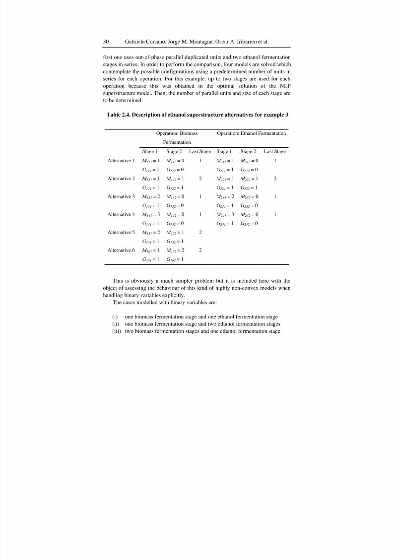
Table 2.4. Description of ethanol superstructure alternatives for example 3
Operation: Biomass
Fermentation
Operation: Ethanol Fermentation
Stage 1 Stage 2 Last Stage Stage 1 Stage 2 Last Stage
Alternative 1 M 111 = 1
G111 = 1
M 112 = 0
G112 = 0
1 M 211 = 1
G211 = 1
M 212 = 0
G212 = 0
1
Alternative 2 M 121 = 1
G121 = 1
M 122 = 1
G122 = 1
2 M 221 = 1
G221 = 1
M 222 = 1
G222 = 1
2
Alternative 3 M 131 = 2
G131 = 1
M 132 = 0
G132 = 0
1 M 231 = 2
G231 = 1
M 232 = 0
G232 = 0
1
Alternative 4 M 141 = 3
G141 = 1
M 142 = 0
G142 = 0
1 M 241 = 3
G241 = 1
M 242 = 0
G242 = 0
1
Alternative 5 M 151 = 2
G151 = 1
M 152 = 1
G152 = 1
2
Alternative 6 M 161 = 1
G161 = 1
M 162 = 2
G162 = 1
2
This is obviously a much simpler problem but it is included here with the
object of assessing the behaviour of this kind of highly non-convex models when
handling binary variables explicitly.
The cases modelled with binary variables are:
(i) one biomass fermentation stage and one ethanol fermentation stage
(ii) one biomass fermentation stage and two ethanol fermentation stages
(iii) two biomass fermentation stages and one ethanol fermentation stage
8/7/2019 Corsano G. Montagna J.M. Iribarren O.A. Aguirre P.A. Mathematical Modeling Approaches for Optimization of Chemic…
http://slidepdf.com/reader/full/corsano-g-montagna-jm-iribarren-oa-aguirre-pa-mathematical-modeling 43/103
NLP Superstructure Modeling for the Optimal Synthesis… 31
(iv) two biomass fermentation stages and two ethanol fermentation stages.
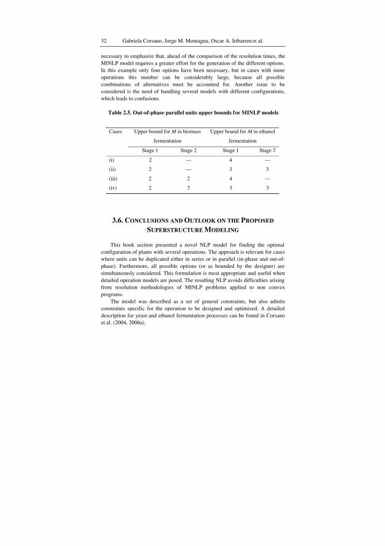
The upper bounds for the M j variables are shown in Table 2.5 for eachpreviously mentioned case. On Table 2.6 the results for each studied case are
shown, including the operations configuration, operating time, unit sizes,
objective function value, number of constraints, number of continuous and
discrete variables and CPU time to achieve the solution.
TL = 5.15 h
TAC = $ 526,822
Feed
EthanolFermentation
G221 = 1M 221 = 1G151 = 1M 151 = 2
BiomassFermentation
Feed
G152 = 1M 152 = 1
BiomassFermentation
BiomassFermentation
Feed
Feed
EthanolFermentation
Feed
Product
G222 = 1M 222 = 1
Operation 1 Operation 2
a = 5 a = 2
Figure 2.6. Optimal solution for PR = 100 kh-1
, β 1=0.3 and β 2=1.
The NLP superstructure model of Example 3 has 1707 continuous variables
and 1617 constraints and the solution was achieved in 10.5 CPU seconds. As it
can be observed, the solutions of the MINLP cases were obtained in a shorter
CPU time, but in all cases the number of constraints and variables is smaller and
the models are much simpler as it was previously mentioned. The solution of the
model (iv) coincides with that obtained in the NLP superstructure model.
A comment on the CPU resolution time is that the differences are not so
significant (of the same order of magnitude). Anyway this depends strongly on
diverse factors, for example the initialization of variables. Nevertheless, it is
8/7/2019 Corsano G. Montagna J.M. Iribarren O.A. Aguirre P.A. Mathematical Modeling Approaches for Optimization of Chemic…
http://slidepdf.com/reader/full/corsano-g-montagna-jm-iribarren-oa-aguirre-pa-mathematical-modeling 44/103
Gabriela Corsano, Jorge M. Montagna, Oscar A. Iribarren et al.32
necessary to emphasize that, ahead of the comparison of the resolution times, the
MINLP model requires a greater effort for the generation of the different options.
In this example only four options have been necessary, but in cases with moreoperations this number can be considerably large, because all possible
combinations of alternatives must be accounted for. Another issue to be
considered is the need of handling several models with different configurations,
which leads to confusions.
Table 2.5. Out-of-phase parallel units upper bounds for MINLP models
Upper bound for M in biomass
fermentation
Upper bound for M in ethanol
fermentation
Cases
Stage 1 Stage 2 Stage 1 Stage 2
(i) 2 --- 4 ---
(ii) 2 --- 3 3
(iii) 2 2 4 ---
(iv) 2 2 3 3
3.6. CONCLUSIONS AND OUTLOOK ON THE PROPOSED
SUPERSTRUCTURE MODELING
This book section presented a novel NLP model for finding the optimal
configuration of plants with several operations. The approach is relevant for cases
where units can be duplicated either in series or in parallel (in-phase and out-of-
phase). Furthermore, all possible options (or as bounded by the designer) are
simultaneously considered. This formulation is most appropriate and useful when
detailed operation models are posed. The resulting NLP avoids difficulties arising
from resolution methodologies of MINLP problems applied to non convexprograms.
The model was described as a set of general constraints, but also admits
constraints specific for the operation to be designed and optimized. A detailed
description for yeast and ethanol fermentation processes can be found in Corsano
et al. (2004, 2006a).
8/7/2019 Corsano G. Montagna J.M. Iribarren O.A. Aguirre P.A. Mathematical Modeling Approaches for Optimization of Chemic…
http://slidepdf.com/reader/full/corsano-g-montagna-jm-iribarren-oa-aguirre-pa-mathematical-modeling 45/103
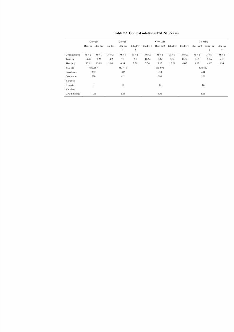
Table 2.6. Optimal solutions of MINLP cases
Case (i) Case (ii) Case (iii)
Bio Fer Etha Fer Bio Fer Etha Fer
1
Etha Fer
2
Bio Fer 1 Bio Fer 2 Etha Fer Bio Fer 1 Bio Fe
Configuration M = 2 M = 1 M = 2 M = 1 M = 1 M = 2 M = 1 M = 1 M = 2 M =
Time (hr) 14.46 7.23 14.2 7.1 7.1 10.64 5.32 5.32 10.32 5.16
Size (m3) 12.6 13.88 5.84 6.39 7.28 7.76 9.15 10.29 4.07 4.17
TAC ($) 643,687 583,410 605,692
Constraints 252 387 359
Continuous
Variables
270 412 384
Discrete
Variables
8 12 12
CPU time (sec) 1.28 2.16 3.71

8/7/2019 Corsano G. Montagna J.M. Iribarren O.A. Aguirre P.A. Mathematical Modeling Approaches for Optimization of Chemic…
http://slidepdf.com/reader/full/corsano-g-montagna-jm-iribarren-oa-aguirre-pa-mathematical-modeling 46/103
NLP Superstructure Modeling for the Optimal Synthesis…34
For the particular operations on which this modeling technique was applied,
the number of alternatives is limited. Indeed, in most cases it is not necessary to
consider all the combinations among the various alternatives of each operationbecause the designer can judge which combinations are feasible for the process
that is being optimized.
This model is simple to write, convergence and good solution are guaranteed
in reasonable CPU time.
8/7/2019 Corsano G. Montagna J.M. Iribarren O.A. Aguirre P.A. Mathematical Modeling Approaches for Optimization of Chemic…
http://slidepdf.com/reader/full/corsano-g-montagna-jm-iribarren-oa-aguirre-pa-mathematical-modeling 47/103
Chapter 4
SYNTHESIS AND DESIGN OF
MULTIPRODUCT/MULTIPURPOSE
BATCH PLANTS:A HEURISTIC APPROACH
FOR DETERMINING MIXED PRODUCT CAMPAIGNS
4.1. INTRODUCTION
In a multiproduct / multipurpose batch plant, several products aremanufactured following the same or different production sequences, sharing the
equipment, raw materials and other production resources. The inherent
operational flexibility of multiproduct / multipurpose plants gives rise to
considerable complexity in the design and synthesis of such plants. In many
published case studies, scheduling strategies are not incorporated or well
integrated. Usually the simplest scheduling sequence, single product campaign, is
considered, which may lead to over-design.
In order to ensure that any resource incorporated in the design can be used as
efficiently as possible, detailed consideration of plant scheduling must be taken
into account at the design stage. Therefore, in this section, the synthesis, designand operational issues for a sequential multipurpose batch plant are considered
simultaneously in an NLP model.
In a sequential multipurpose plant a specific direction in the plant floor is
recognized that is followed by the production paths of all the products (Voudouris
and Grossmann, 1996). However some processing units are used only by some
8/7/2019 Corsano G. Montagna J.M. Iribarren O.A. Aguirre P.A. Mathematical Modeling Approaches for Optimization of Chemic…
http://slidepdf.com/reader/full/corsano-g-montagna-jm-iribarren-oa-aguirre-pa-mathematical-modeling 48/103
Gabriela Corsano, Jorge M. Montagna, Oscar A. Iribarren et al.36
products. Obviously, the model presented is also valid for the multiproduct batch
plant where all the products use all the stages. Besides, alternatives for the number
of units in series are introduced. The configuration options are explicitlyconsidered in terms of a superstructure as was presented in the previous section.
The simultaneous optimization of several problems is not an usual approach
in the chemical engineering literature. In general, these problems are treated in
separate form: first the plant configuration problem, then the sizing problem and
lastly the campaign determination problem. This leads to sub-optimal solutions.
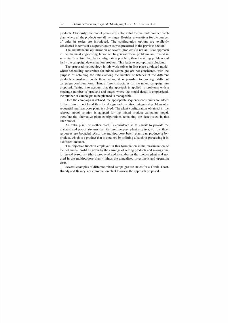
The proposed methodology in this work solves in first place a relaxed model
where scheduling constraints for mixed campaigns are not considered, with the
purpose of obtaining the ratios among the number of batches of the different
products considered. With these ratios, it is possible to envisage different
campaign configurations. Then, different structures for the mixed campaign areproposed. Taking into account that the approach is applied to problems with a
moderate number of products and stages where the model detail is emphasized,
the number of campaigns to be planned is manageable.
Once the campaign is defined, the appropriate sequence constraints are added
to the relaxed model and thus the design and operation integrated problem of a
sequential multipurpose plant is solved. The plant configuration obtained in the
relaxed model solution is adopted for the mixed product campaign model,
therefore the alternative plant configurations remaining are deactivated in this
later model.
An extra plant, or mother plant, is considered in this work to provide the
material and power streams that the multipurpose plant requires, so that these
resources are bounded. Also, the multipurpose batch plant can produce a by-
product, which is a product that is obtained by splitting a batch or processing it in
a different manner.
The objective function employed in this formulation is the maximization of
the net annual profit as given by the earnings of selling products and savings due
to unused resources (those produced and available in the mother plant and not
used in the multipurpose plant), minus the annualized investment and operating
costs.
Several examples of different mixed campaigns are stated for a Torula Yeast,
Brandy and Bakery Yeast production plant to assess the approach proposed.
8/7/2019 Corsano G. Montagna J.M. Iribarren O.A. Aguirre P.A. Mathematical Modeling Approaches for Optimization of Chemic…
http://slidepdf.com/reader/full/corsano-g-montagna-jm-iribarren-oa-aguirre-pa-mathematical-modeling 49/103
Synthesis and Design of Multiproduct/Multipurpose Batch Plants 37
4.2. MODEL ASSUMPTIONS
The problem considered here has the following characteristics:
(i) The plant has batch and semi-continuous units.
(ii) N p products are processed in the plant.
U1 U2 U3
Raw material 1
U4 U5
Product A
Product B
Product C
Feeding Feeding
Legend A production pathB production pathC production path, sub-product of BMaterial recycles
Raw material 2
Figure 3.1. Flowsheet of a sequential multipurpose batch plant.
(iii) Not all the products follow the same production path, i.e. a sequential
multipurpose batch plant is considered (Figure 3.1).(iv) The production path for each product is known.
(v) The product demands are upper and lower bounded.
(vi) The processing times are continuous variables and the horizon time is
given.
(vii) The mixing, splitting and recycle of batches are allowed.
(viii) The production of by-products is also considered.
(ix) The material and energy resources are bounded.
(x) The unit sizes are continuous variables
The objective is to determine the optimal plant design and operation to meet aspecified economic criterion.
Figure 3.1 shows a sequential multipurpose plant where two products, A and
B, and a by-product of B, product C are produced. Product A follows the
production path U1→ U4 and U1 receives an extra feed (blend of batches) and a
8/7/2019 Corsano G. Montagna J.M. Iribarren O.A. Aguirre P.A. Mathematical Modeling Approaches for Optimization of Chemic…
http://slidepdf.com/reader/full/corsano-g-montagna-jm-iribarren-oa-aguirre-pa-mathematical-modeling 50/103
Gabriela Corsano, Jorge M. Montagna, Oscar A. Iribarren et al.38
recycled batch from U4. Product B follows the path U1→ U2→ U3→ U4. At U3
batches are split to produce product C through U5. U3 also has an extra feed.
4.3. SOLUTION PROCEDURE
The simultaneous optimization of the synthesis, design, operation and
scheduling of a sequential multipurpose batch plant, results in a very large size
problem, difficult to solve as was pointed in the introduction section. So, a
heuristic procedure is proposed in order to solve this simultaneous optimization.
The main idea lies in solving first a model without mixed product campaign
constraints and then, according to the optimal number of batches of each product
obtained in the first model solution, determining the possible campaignconfigurations. For each campaign configuration proposed, an NLP model is
formulated for the optimal plant configuration obtained in the first model solution.
The heuristic approach is resumed in the following steps:
(i) First, a model whose constraints consider the design and operation of a
multipurpose plant without considering the tasks scheduling constraints is
solved. This model is a relaxation of the mixed campaigns problem and is
solved as an NLP problem. The model has an embedded superstructure
that considers different configuration options for the plant synthesis. The
solution of the relaxed model provides the estimated number of batchesof each product and the plant configuration.
(ii) Relationships between the number of batches of each product, which are
obtained from the relaxed model are established, and the possible
sequences of the multiproduct campaigns are selected for the plant
synthesis obtained in the relaxed model solution.
(iii) For each proposed campaign configuration, an NLP problem is modelled
and solved. In this model, a novel set of tasks scheduling constraints are
added to the relaxed model in order to ensure that the production
processes of two different products do not overlap in the same unit. In
this way, a model for each mixed product campaign is formulated andsolved, with the optimal plant configuration obtained from the relaxed
model solution. At this step, the plant configuration is fixed and the
sizing problem is solved.
(iv) The campaign with the best objective function value is chosen as the
optimal solution.
8/7/2019 Corsano G. Montagna J.M. Iribarren O.A. Aguirre P.A. Mathematical Modeling Approaches for Optimization of Chemic…
http://slidepdf.com/reader/full/corsano-g-montagna-jm-iribarren-oa-aguirre-pa-mathematical-modeling 51/103
Synthesis and Design of Multiproduct/Multipurpose Batch Plants 39
(v) The first model represents a relaxation for the second one. Therefore, the
objective function value of the relaxed model solution represents an
upper bound for the objective value of the mixed product campaignmodel. In the studied cases presented below, the gap between these
values is very tight, which ensures that the solution obtained for the
mixed product campaign is the optimal.
4.4. MATHEMATICAL MODELING
A plant with N j batch units and N k semi-continuous units is considered. N p
products are manufactured in the plant, which do not necessarily follow the same
production path.Both problems (the relaxed one and the problem with scheduling constraints)
include a detailed modeling for all the products and the batch and semi-continuous
units.
4.4.1. Relaxed Model
The components and total mass balances at each stage, the connection
constraints between stages and the design equations for each stage for each
product are considered as a detailed model. If there are recycles orinterconnections between the production processes, as it really happens in the
study cases, also the balances that correspond to these connections are considered.
Mass balances for some units are given by differential equations such as
x xt hdt
dC xij ∀= ),( (3.1)
where C xij is the concentration of component x (biomass, substrate, product, etc.),
at stage j of the production process of product i. These dynamic equations are
discretized and included in the overall model. Note that the discretized equations
involve the processing time of the batch item and the time integration step, all of
which are considered variables. The number of grid points is a problem data, but
as the final processing time is variable, the discretization step length is also an
optimization variable determined according to the final time for each unit. For
8/7/2019 Corsano G. Montagna J.M. Iribarren O.A. Aguirre P.A. Mathematical Modeling Approaches for Optimization of Chemic…
http://slidepdf.com/reader/full/corsano-g-montagna-jm-iribarren-oa-aguirre-pa-mathematical-modeling 52/103
Gabriela Corsano, Jorge M. Montagna, Oscar A. Iribarren et al.40
these models, the trapezoidal method was adopted (Atkinson, 1989). For example,
if the biomass balance is
( ) ijijij
ijX
dt
dX υ μ −= (3.2)
where X represents the biomass concentration, the specific growth rate of
biomass, and υ the biomass death rate, the corresponding set of algebraic
equations is
( ) ( )( )
( 1) ( ) ( 1) ( 1) ( ) ( )
2
ijp p p p p p
ij ij ij ij ij ij ij ij
lX X X X μ υ μ υ + + += + − + − (3.3)
where l is the step length and p = 1, …, P are the grid points.
In addition, for the stages that are shared by several products, the following
constraints are considered.
For batch item j and product i:
ipijj EBjN i V V ∈∀=∀≥ ,,...,1 (3.4)
For semi-continuous item k and product i:
1,..., ,k ik p i
V V i N k ES≥ ∀ = ∀ ∈ (3.5)
where V are the batch and semi-continuous unit sizes and EBi and ESi represent
the set of batch and semi-continuous units in the production path of product i. In
both cases the unit size, V j or V k , assures to process the required volume V ij or V ik ,
for all products.
Let t ij be the processing time for product i at stage j, ik θ the processing time
for product i at semi-continuous stage k , CT i the cycle time for the production of
product i and Nbi the number of batches of product i over the horizon time HT ,
then
' '' 1,..., ,ij ik ij ik p i
T t i N j EBθ θ = + + ∀ = ∀ ∈ (3.6)
8/7/2019 Corsano G. Montagna J.M. Iribarren O.A. Aguirre P.A. Mathematical Modeling Approaches for Optimization of Chemic…
http://slidepdf.com/reader/full/corsano-g-montagna-jm-iribarren-oa-aguirre-pa-mathematical-modeling 53/103
Synthesis and Design of Multiproduct/Multipurpose Batch Plants 41
1,...,i ij p i
CT T i N j EB≥ ∀ = ∀ ∈ (3.7)
Note that Eq. (3.6) defines the time that the batch unit j will be occupied with
product i, which contemplates the material loading ( 'ik θ ) and unloading ( ''ik θ )
time if this unit is located between semi-continuous units. In this approach
variables t ij and 'ik θ are assumed to be involved in detailed sub-models, some of
them written as differential equations and included in the actual model as was
presented in equations (3.1)-(3.3).
Several consecutive semi-continuous units give rise to a semi-continuous sub-
train. In this paper, only perfectly synchronized semi-continuous sub-trains are
considered, then:
, 1 1,...,ik i k p
i N θ θ += ∀ = (3.8)
where k and k +1 belong to the same sub-train.
For products i that share the unit j (i∈ I j) the following constraints are
considered:
j
i ij
i I
Nb T HT ∈
≤∑ 1,...,j
j N ∀ = (3.9)
In the same way, for all the products i that share the unit k (k ∈ I k )
k
i ik
i I
Nb HT θ ∈
≤∑ 1,...,k
k N ∀ = (3.10)
In this way the available time is not exceeded.
If all the products follow the same production path, then Eq. (3.10) becomes
redundant because the batch processing time considers the semi-continuous
processing times upstream and downstream of the batch unit.
A characteristic of this model is that, for certain batch stages, the number of
units in series is a priori unknown. For these stages, a superstructure thatcontemplates all the possible configurations (or those chosen by the designer as
feasible) is modelled and embedded in the global model, as was described in
Section 2. Then, if the stage is preceded by a semi-continuous unit, the first unit in
the series must include the filling time in its operating time, or the emptying time
if this stage has a downstream semi continuous unit (see Figure 3.2).
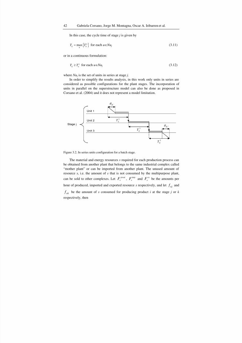
8/7/2019 Corsano G. Montagna J.M. Iribarren O.A. Aguirre P.A. Mathematical Modeling Approaches for Optimization of Chemic…
http://slidepdf.com/reader/full/corsano-g-montagna-jm-iribarren-oa-aguirre-pa-mathematical-modeling 54/103
Gabriela Corsano, Jorge M. Montagna, Oscar A. Iribarren et al.42
In this case, the cycle time of stage j is given by
{ }maxu
ij ijuT T = for each u∈Nuj (3.11)
or in a continuous formulation:
u
ij ijT T ≥ for each u∈Nuj (3.12)
where Nuj is the set of units in series at stage j.
In order to simplify the results analysis, in this work only units in series are
considered as possible configurations for the plant stages. The incorporation of
units in parallel on the superstructure model can also be done as proposed inCorsano et al. (2004) and it does not represent a model limitation.
1ijT
2ijT
3ijT
Stage j
Unit 1
Unit 2
Unit 3
'ik θ
''ik θ
Figure 3.2. In series units configuration for a batch stage.
The material and energy resources s required for each production process can
be obtained from another plant that belongs to the same industrial complex called
“mother plant” or can be imported from another plant. The unused amount of
resource s, i.e. the amount of s that is not consumed by the multipurpose plant,
can be sold to other complexes. Let
prod
sF ,
imp
sF and
ex
sF be the amounts perhour of produced, imported and exported resource s respectively, and let
sijf and
sik f be the amount of s consumed for producing product i at the stage j or k
respectively, then
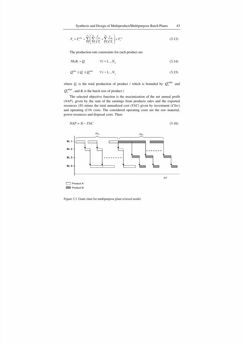
8/7/2019 Corsano G. Montagna J.M. Iribarren O.A. Aguirre P.A. Mathematical Modeling Approaches for Optimization of Chemic…
http://slidepdf.com/reader/full/corsano-g-montagna-jm-iribarren-oa-aguirre-pa-mathematical-modeling 55/103
Synthesis and Design of Multiproduct/Multipurpose Batch Plants 43
1 1 1
p j k N N N
sijimp exsik
s s s
i j k i i
f f F F F
CT CT = = =
⎛ ⎞+ = + +⎜ ⎟⎜ ⎟
⎝ ⎠∑ ∑ ∑ (3.13)
The production rate constraints for each product are
1i i i pNb B Q i ,..,N = ∀ = (3.14)
min max 1i i i p
Q Q Q i ,..,N ≤ ≤ ∀ = (3.15)
where Qi is the total production of product i which is bounded byminiQ and
maxiQ , and Bi is the batch size of product i.
The selected objective function is the maximization of the net annual profit
(NAP), given by the sum of the earnings from products sales and the exported
resources (Sl) minus the total annualized cost (TAC ) given by investment (CInv)
and operating (CO) costs. The considered operating costs are the raw material,
power resources and disposal costs. Then:
NAP = Sl – TAC (3.16)
NbA NbB
St. 1
St. 2
St. 3
St. 4
HT
Product A
Product B
Figure 3.3. Gantt chart for multipurpose plant relaxed model.
8/7/2019 Corsano G. Montagna J.M. Iribarren O.A. Aguirre P.A. Mathematical Modeling Approaches for Optimization of Chemic…
http://slidepdf.com/reader/full/corsano-g-montagna-jm-iribarren-oa-aguirre-pa-mathematical-modeling 56/103
Gabriela Corsano, Jorge M. Montagna, Oscar A. Iribarren et al.44
exp
i 1 s
pN
i i s sSl G Q G F HT
=
= +∑ ∑ (3.17)
where Gi represents the product i sale price ($ ton-1), Gs the resource price of s ($
ton-1) andexp
sF the amount of unused resource s (ton).
TAC CInv CO= + (3.18)
j k
ann j j k k
j k
CInv C V V β β
α α ⎛ ⎞
= +⎜ ⎟⎝ ⎠∑ ∑ (3.19)
1
pN
prod prod imp imp
i i s s s s
i s s
CO Nb Res HT C F C F =
⎛ ⎞= + +⎜ ⎟
⎝ ⎠∑ ∑ ∑ (3.20)
α j, β j, α k , and β k are cost coefficients for units, C s is the cost of resource s,
and Resi the disposal cost of product process i that varies according to the effluent.
The relaxed model solution provides the optimal plant configuration and
design and the number of batches of each product to be produced.
It is worth noting that the relaxed model resembles a single product campaign
one, in which all the batches of a product are processed without overlapping with
others products. The difference is that in the relaxed model, the schedulingconstraint of a single campaign model
1
pN
i i
i
CT Nb HT =
≤∑
is not necessarily satisfied because of Eq. (3.9).
Figure 3.3 schematizes the relaxed model solution of a plant that processes
two products with different production paths. Product A follows the path Stage 1
→ Stage 2 → Stage 4, while product B follows the path Stage 1 → Stage 3 → Stage 4.
8/7/2019 Corsano G. Montagna J.M. Iribarren O.A. Aguirre P.A. Mathematical Modeling Approaches for Optimization of Chemic…
http://slidepdf.com/reader/full/corsano-g-montagna-jm-iribarren-oa-aguirre-pa-mathematical-modeling 57/103
Synthesis and Design of Multiproduct/Multipurpose Batch Plants 45
4.4.2. Multiproduct Campaign Model
In many cases, a stream in the production of a product can be recycled to aprevious stage in the processing of the same or another product. In such cases the
single product campaign is impracticable because the material to be recycled
should be stored. In addition single product campaigns require high inventory
levels. Furthermore many products cannot be stored because they are degraded.
From the point of view of the mathematical model, greater challenges arise than in
the formulations for single campaigns. The first decision to be considered is how
the multiproduct campaign will be configured. In this work this decision is
imposed by the designer from the estimation of the ratio of number of batches of
the different products elaborated in the plant.
Let i’ be the product with the small number of batches in the relaxed model
solution. Let'
i
i
i
Nbr round
Nb
⎛ ⎞= ⎜ ⎟
⎝ ⎠be the rounding of the relation between the
number of batches of each product i and product i’, obtained in the relaxed model
solution, so that r i is a model parameter.
Let Nb be the number of times that the mixed campaign is repeated. For the
mixed campaign model, the following constraints are imposed:
Nb = Nbi’ (3.21)
Nb= Nbi 1−
ir pN i ,...,1=∀ (3.22)
Nb is an optimization variable since Nbi is an optimization variable for each
product i.
For example, if three products A, B and C are processed in the sequential
multipurpose plant with N A = 100, N B = 120 y N C = 310 in the relaxed model
solution, then:
Nb = N A, r B = 1 y r C = 3, i.e. the campaign A-B-C-C-C or some of its
permutations is established.
Given that this strategy is here applied to detailed models with a reducednumber of products, this is an affordable approach. Therefore, this procedure
estimates the proportion among the number of batches of all products. Different
campaigns can be proposed by the designer.
Now, new constraints have to be developed to formulate the different
conditions that arise when mixed campaigns are used. All the following
constraints are posed for a determined mixed campaign.
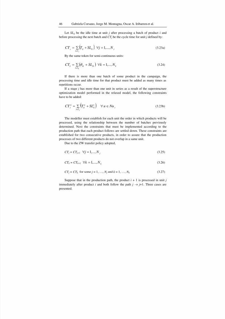
8/7/2019 Corsano G. Montagna J.M. Iribarren O.A. Aguirre P.A. Mathematical Modeling Approaches for Optimization of Chemic…
http://slidepdf.com/reader/full/corsano-g-montagna-jm-iribarren-oa-aguirre-pa-mathematical-modeling 58/103
Gabriela Corsano, Jorge M. Montagna, Oscar A. Iribarren et al.46
Let SLij be the idle time at unit j after processing a batch of product i and
before processing the next batch and CT j be the cycle time for unit j defined by:
( )∑ +=∈ jI i
ijijj SLT CT jN j ,...,1=∀ (3.23a)
By the same token for semi-continuous units:
( )∑ +=∈ k I i
ik ik k SLCT θ k N k ,...,1=∀ (3.24)
If there is more than one batch of some product in the campaign, the
processing time and idle time for that product must be added as many times as
repetitions occur.If a stage j has more than one unit in series as a result of the superstructure
optimization model performed in the relaxed model, the following constraints
have to be added:
) jI i
u
ij
u
ij
u
j Nuu SLT CT j
∈∀∑ +=∈
(3.23b)
The modeller must establish for each unit the order in which products will be
processed, using the relationship between the number of batches previously
determined. Next the constraints that must be implemented according to the
production path that each product follows are settled down. These constraints are
established for two consecutive products, in order to assure that the production
processes of two different products do not overlap in a same unit.
Due to the ZW transfer policy adopted,
CT j = CT j+1 jN j ,...,1=∀ (3.25)
CT k = CT k+1 k N k ,...,1=∀ (3.26)
CT j = CT k for some j = 1, …, N j and k = 1, …, N k (3.27)
Suppose that in the production path, the product i + 1 is processed in unit j
immediately after product i and both follow the path j → j+1. Three cases are
presented.
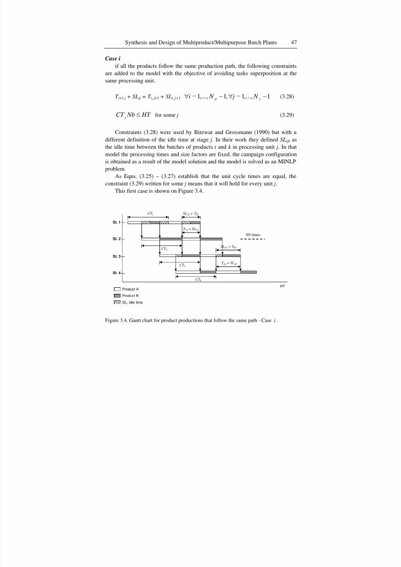
8/7/2019 Corsano G. Montagna J.M. Iribarren O.A. Aguirre P.A. Mathematical Modeling Approaches for Optimization of Chemic…
http://slidepdf.com/reader/full/corsano-g-montagna-jm-iribarren-oa-aguirre-pa-mathematical-modeling 59/103
Synthesis and Design of Multiproduct/Multipurpose Batch Plants 47
Case i
if all the products follow the same production path, the following constraints
are added to the model with the objective of avoiding tasks superposition at thesame processing unit.
T i+1,j + SLij = T i,,j+1 + SLi,,j+1 1,...,1,1,...,1 −=∀−=∀ jp N jN i (3.28)
HT NbCT j ≤ for some j (3.29)
Constraints (3.28) were used by Birewar and Grossmann (1990) but with a
different definition of the idle time at stage j. In their work they defined SLijk as
the idle time between the batches of products i and k in processing unit j. In thatmodel the processing times and size factors are fixed, the campaign configuration
is obtained as a result of the model solution and the model is solved as an MINLP
problem.
As Eqns. (3.25) – (3.27) establish that the unit cycle times are equal, the
constraint (3.29) written for some j means that it will hold for every unit j.
This first case is shown on Figure 3.4.
SLij idle time
Product A
Product B
St. 2
St. 1
St. 3
St. 4
HT
Nb times
CT 1
CT 4
T A2 + SLA2
SLA1 + T B1
CT 3 T A4 + SLA4
SLA3 + T B3 CT 2
Figure 3.4. Gantt chart for product productions that follow the same path - Case i.
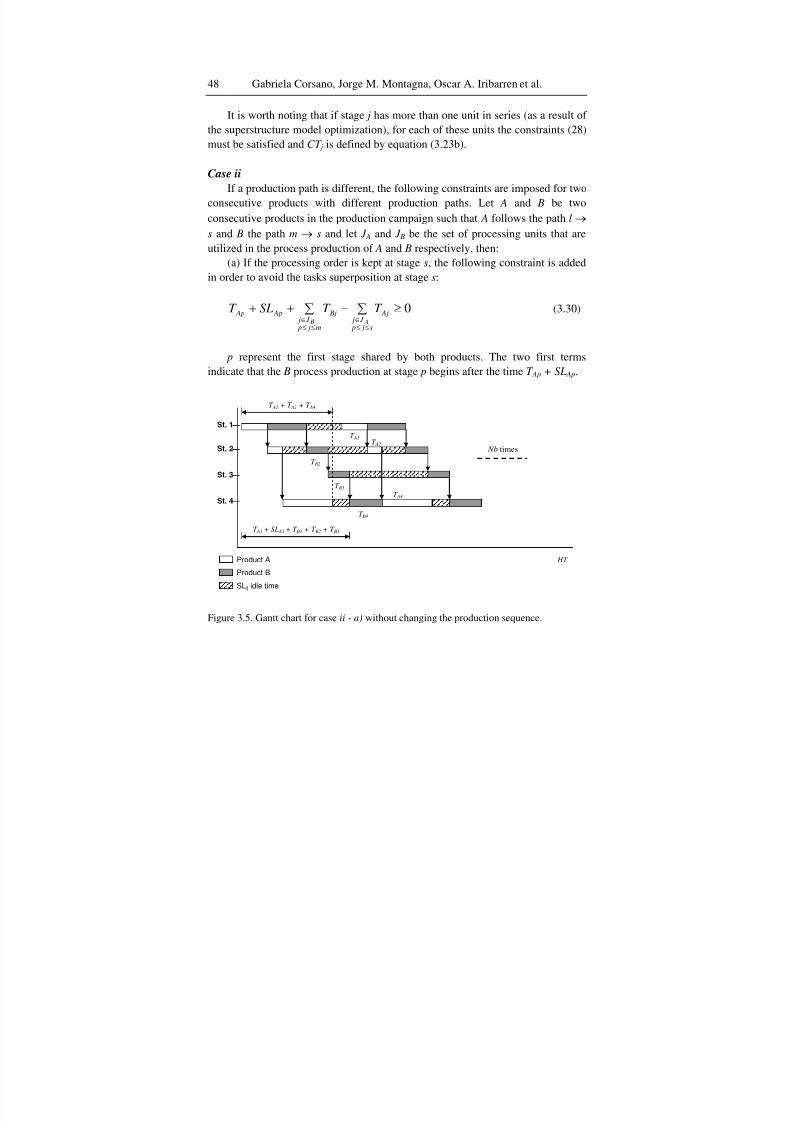
8/7/2019 Corsano G. Montagna J.M. Iribarren O.A. Aguirre P.A. Mathematical Modeling Approaches for Optimization of Chemic…
http://slidepdf.com/reader/full/corsano-g-montagna-jm-iribarren-oa-aguirre-pa-mathematical-modeling 60/103
Gabriela Corsano, Jorge M. Montagna, Oscar A. Iribarren et al.48
It is worth noting that if stage j has more than one unit in series (as a result of
the superstructure model optimization), for each of these units the constraints (28)
must be satisfied and CT j is defined by equation (3.23b).
Case ii
If a production path is different, the following constraints are imposed for two
consecutive products with different production paths. Let A and B be two
consecutive products in the production campaign such that A follows the path l →
s and B the path m → s and let J A and J B be the set of processing units that are
utilized in the process production of A and B respectively, then:
(a) If the processing order is kept at stage s, the following constraint is added
in order to avoid the tasks superposition at stage s:
0≥∑−∑++≤≤
∈≤≤
∈sjp
J jAj
mjpJ j
BjApApAB
T T SLT (3.30)
p represent the first stage shared by both products. The two first terms
indicate that the B process production at stage p begins after the time T Ap + SLAp.
St. 1
St. 2
St. 3
St. 4
HT
Nb times
SLij idle time
T A1 T A2
T A4
T A1 + T A2 + T A4
T B2
T B3
T B4
T A1 + SLA1 + T B1 + T B2 + T B3
Product A
Product B
Figure 3.5. Gantt chart for case ii - a) without changing the production sequence.
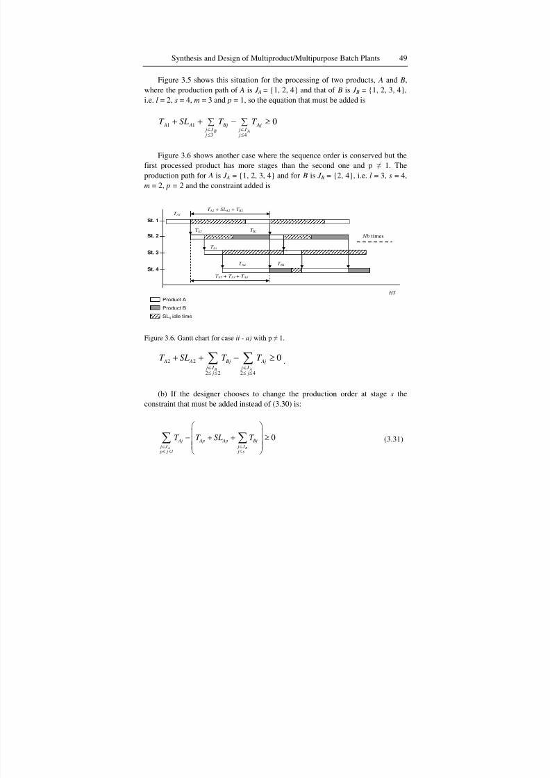
8/7/2019 Corsano G. Montagna J.M. Iribarren O.A. Aguirre P.A. Mathematical Modeling Approaches for Optimization of Chemic…
http://slidepdf.com/reader/full/corsano-g-montagna-jm-iribarren-oa-aguirre-pa-mathematical-modeling 61/103
Synthesis and Design of Multiproduct/Multipurpose Batch Plants 49
Figure 3.5 shows this situation for the processing of two products, A and B,
where the production path of A is J A = {1, 2, 4} and that of B is J B = {1, 2, 3, 4},
i.e. l = 2, s = 4, m = 3 and p = 1, so the equation that must be added is
0
43
11 ≥∑−∑++≤∈
≤∈
jJ j
Aj
jJ j
BjAAAB
T T SLT
Figure 3.6 shows another case where the sequence order is conserved but the
first processed product has more stages than the second one and p ≠ 1. The
production path for A is J A = {1, 2, 3, 4} and for B is J B = {2, 4}, i.e. l = 3, s = 4,
m = 2, p = 2 and the constraint added is
St. 1
St. 2
St. 3
St. 4
HT
Nb times
SLij idle time
T A1
T A2 + T A3 + T A4
Product A
Product B
T A2
T A4
T A3
T B2
T B4
T A2 + SLA2 + T B2
Figure 3.6. Gantt chart for case ii - a) with p ≠ 1.
2 2
2 2 2 4
0B A
A A Bj Aj
j J j J j j
T SL T T ∈ ∈≤ ≤ ≤ ≤
+ + − ≥∑ ∑ .
(b) If the designer chooses to change the production order at stage s the
constraint that must be added instead of (3.30) is:
0A B
Aj Ap Ap Bj
j J j J p j l j s
T T SL T ∈ ∈≤ ≤ ≤
⎛ ⎞⎜ ⎟− + + ≥⎜ ⎟⎜ ⎟⎝ ⎠
∑ ∑ (3.31)
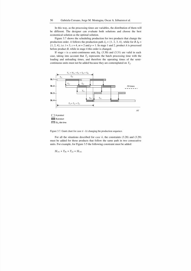
8/7/2019 Corsano G. Montagna J.M. Iribarren O.A. Aguirre P.A. Mathematical Modeling Approaches for Optimization of Chemic…
http://slidepdf.com/reader/full/corsano-g-montagna-jm-iribarren-oa-aguirre-pa-mathematical-modeling 62/103
Gabriela Corsano, Jorge M. Montagna, Oscar A. Iribarren et al.50
In this way, as the processing times are variables, the distribution of them will
be different. The designer can evaluate both solutions and choose the best
economical solution as the optimal solution.Figure 3.7 shows the scheduling production for two products that change the
production order. A follows the production path J A = {1, 2, 3, 4}, while for B J B =
{1, 2, 4}, i.e. l = 3, s = 4, m = 2 and p = 1. In stage 1 and 2, product A is processed
before product B, while in stage 4 this order is changed.
If stage s is a semi-continuous unit, Eq. (3.30) and (3.31) are valid in each
case, taking into account that T ij represents the batch processing time with the
loading and unloading times, and therefore the operating times of the semi-
continuous units must not be added because they are contemplated on T ij.
St. 1
St. 2
St. 3
St. 4
HT
Nb times
SLij idle time
T A1+ T A2 + T A3
A product
B product
T A1
T A2
T A4
T A3
T B1
T B2
T B4
T A1 + SLA1 +T B1 + T B2 + T B4
Figure 3.7. Gantt chart for case ii - b) changing the production sequence.
For all the situations described for case ii, the constraints (3.28) and (3.29)
must be added for those products that follow the same path in two consecutive
units. For example, for Figure 3.5 the following constraint must be added:
SLA1 + T B1 = T A2 + SLA2
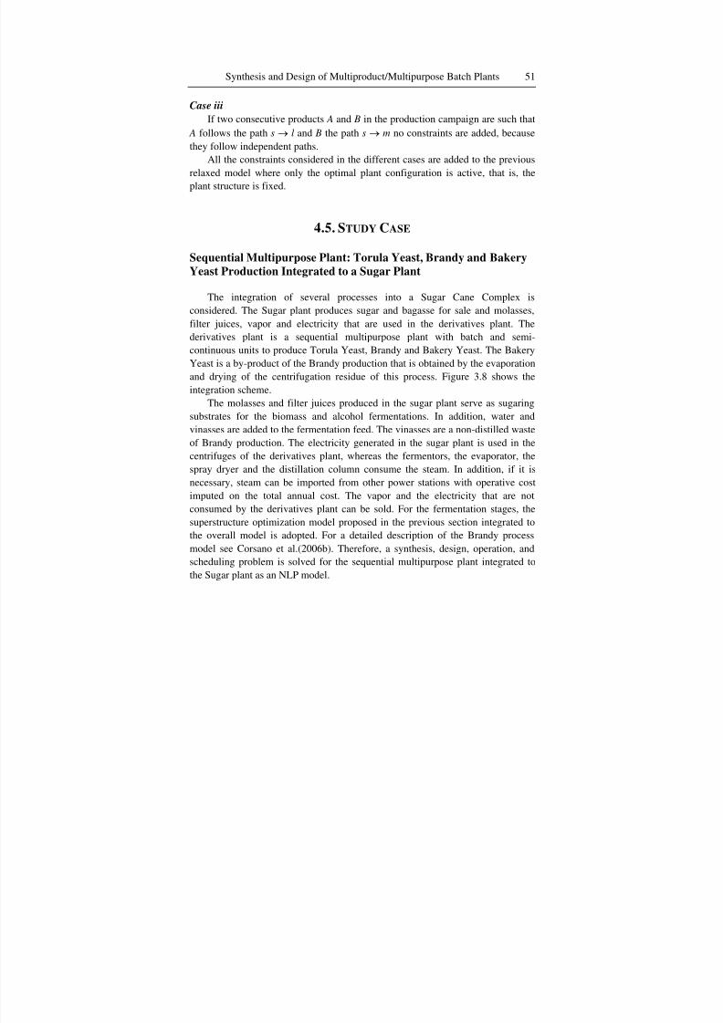
8/7/2019 Corsano G. Montagna J.M. Iribarren O.A. Aguirre P.A. Mathematical Modeling Approaches for Optimization of Chemic…
http://slidepdf.com/reader/full/corsano-g-montagna-jm-iribarren-oa-aguirre-pa-mathematical-modeling 63/103
Synthesis and Design of Multiproduct/Multipurpose Batch Plants 51
Case iii
If two consecutive products A and B in the production campaign are such that
A follows the path s → l and B the path s → m no constraints are added, becausethey follow independent paths.
All the constraints considered in the different cases are added to the previous
relaxed model where only the optimal plant configuration is active, that is, the
plant structure is fixed.
4.5. STUDY CASE
Sequential Multipurpose Plant: Torula Yeast, Brandy and Bakery
Yeast Production Integrated to a Sugar Plant
The integration of several processes into a Sugar Cane Complex is
considered. The Sugar plant produces sugar and bagasse for sale and molasses,
filter juices, vapor and electricity that are used in the derivatives plant. The
derivatives plant is a sequential multipurpose plant with batch and semi-
continuous units to produce Torula Yeast, Brandy and Bakery Yeast. The Bakery
Yeast is a by-product of the Brandy production that is obtained by the evaporation
and drying of the centrifugation residue of this process. Figure 3.8 shows the
integration scheme.
The molasses and filter juices produced in the sugar plant serve as sugaringsubstrates for the biomass and alcohol fermentations. In addition, water and
vinasses are added to the fermentation feed. The vinasses are a non-distilled waste
of Brandy production. The electricity generated in the sugar plant is used in the
centrifuges of the derivatives plant, whereas the fermentors, the evaporator, the
spray dryer and the distillation column consume the steam. In addition, if it is
necessary, steam can be imported from other power stations with operative cost
imputed on the total annual cost. The vapor and the electricity that are not
consumed by the derivatives plant can be sold. For the fermentation stages, the
superstructure optimization model proposed in the previous section integrated to
the overall model is adopted. For a detailed description of the Brandy processmodel see Corsano et al.(2006b). Therefore, a synthesis, design, operation, and
scheduling problem is solved for the sequential multipurpose plant integrated to
the Sugar plant as an NLP model.
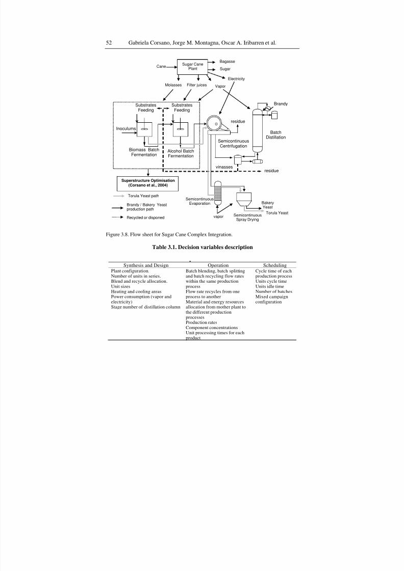
8/7/2019 Corsano G. Montagna J.M. Iribarren O.A. Aguirre P.A. Mathematical Modeling Approaches for Optimization of Chemic…
http://slidepdf.com/reader/full/corsano-g-montagna-jm-iribarren-oa-aguirre-pa-mathematical-modeling 64/103
Gabriela Corsano, Jorge M. Montagna, Oscar A. Iribarren et al.52
Brandy
Inoculums
SubstratesFeeding
residue
SubstratesFeeding
Biomass BatchFermentation
Alcohol BatchFermentation
SemicontinuousCentrifugation
BatchDistillation
vinassesresidue
Superstructure Optimisation(Corsano et al., 2004)
Sugar CanePlant
Cane
Bagasse
Sugar
Molasses Filter juices Vapor
Electricity
SemicontinuousEvaporation
SemicontinuousSpray Drying
vapor
Torula Yeast path
Brandy / Bakery Yeastproduction path
Recycled or disponed
BakeryYeast
Torula Yeast
Figure 3.8. Flow sheet for Sugar Cane Complex Integration.
Table 3.1. Decision variables description
Synthesis and Design Operation SchedulingPlant configuration.Number of units in series.Blend and recycle allocation.Unit sizesHeating and cooling areasPower consumption (vapor andelectricity)Stage number of distillation column
Batch blending, batch splittingand batch recycling flow rateswithin the same productionprocessFlow rate recycles from oneprocess to anotherMaterial and energy resourcesallocation from mother plant tothe different productionprocessesProduction ratesComponent concentrationsUnit processing times for eachproduct
Cycle time of eachproduction processUnits cycle timeUnits idle timeNumber of batchesMixed campaignconfiguration
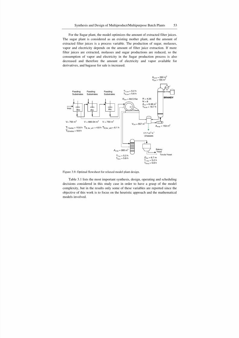
8/7/2019 Corsano G. Montagna J.M. Iribarren O.A. Aguirre P.A. Mathematical Modeling Approaches for Optimization of Chemic…
http://slidepdf.com/reader/full/corsano-g-montagna-jm-iribarren-oa-aguirre-pa-mathematical-modeling 65/103
Synthesis and Design of Multiproduct/Multipurpose Batch Plants 53
For the Sugar plant, the model optimizes the amount of extracted filter juices.
The sugar plant is considered as an existing mother plant, and the amount of
extracted filter juices is a process variable. The production of sugar, molasses,vapor and electricity depends on the amount of filter juice extraction. If more
filter juices are extracted, molasses and sugar productions are reduced, so the
consumption of vapor and electricity in the Sugar production process is also
decreased and therefore the amount of electricity and vapor available for
derivatives, and bagasse for sale is increased.
Feeding
Substrates
Bio Alc Alc
Aevap = 265 m2
TT,ev = 5.2 h
TB,ev = 5.8 h
V= 750 m3
TT,ferbio = 10.8 h
TB,ferbio = 9.8 h
V = 660.54 m3
TB, fer_al1 = 4.8 h
TT,cen= 5.2 h
TB,cen= 5.8 h
Rcen = 84.5 Kw
Acond = 260 m2
VDR = 155 m3
R = 4.25
N = 8
Acol = 6.38 m2
TB,dis = 18.7 h
17.7 m3 h-1
vinasses
Aevap = 153 m2
VVR = 557 m3
Feeding
Substrates
Feeding
Substrates
V = 750 m3
TB,fer_al2 = 6.1 h
D sec = 6.7 m
TT,dry = 5.2 h
TB,dry = 5.8 h
Inoc
BakeryYeast
Torula Yeast
BRANDY
Figure 3.9. Optimal flowsheet for relaxed model plant design.
Table 3.1 lists the most important synthesis, design, operating and scheduling
decisions considered in this study case in order to have a grasp of the model
complexity, but in the results only some of these variables are reported since the
objective of this work is to focus on the heuristic approach and the mathematical
models involved.
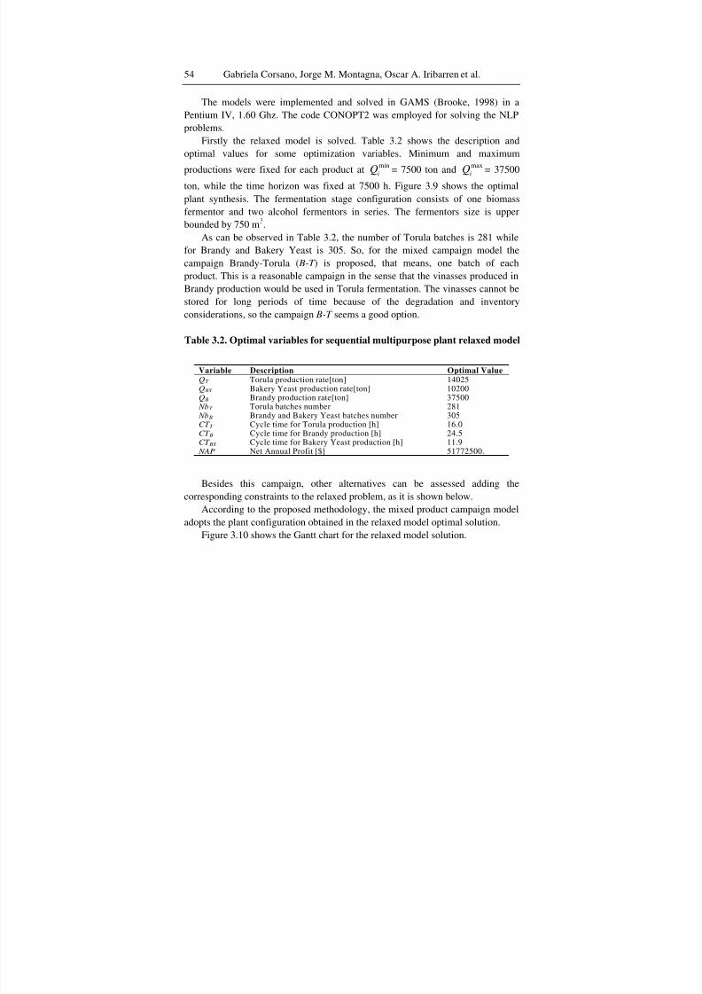
8/7/2019 Corsano G. Montagna J.M. Iribarren O.A. Aguirre P.A. Mathematical Modeling Approaches for Optimization of Chemic…
http://slidepdf.com/reader/full/corsano-g-montagna-jm-iribarren-oa-aguirre-pa-mathematical-modeling 66/103
Gabriela Corsano, Jorge M. Montagna, Oscar A. Iribarren et al.54
The models were implemented and solved in GAMS (Brooke, 1998) in a
Pentium IV, 1.60 Ghz. The code CONOPT2 was employed for solving the NLP
problems.Firstly the relaxed model is solved. Table 3.2 shows the description and
optimal values for some optimization variables. Minimum and maximum
productions were fixed for each product atmin
iQ = 7500 ton andmax
iQ = 37500
ton, while the time horizon was fixed at 7500 h. Figure 3.9 shows the optimal
plant synthesis. The fermentation stage configuration consists of one biomass
fermentor and two alcohol fermentors in series. The fermentors size is upper
bounded by 750 m3.
As can be observed in Table 3.2, the number of Torula batches is 281 while
for Brandy and Bakery Yeast is 305. So, for the mixed campaign model the
campaign Brandy-Torula (B-T ) is proposed, that means, one batch of eachproduct. This is a reasonable campaign in the sense that the vinasses produced in
Brandy production would be used in Torula fermentation. The vinasses cannot be
stored for long periods of time because of the degradation and inventory
considerations, so the campaign B-T seems a good option.
Table 3.2. Optimal variables for sequential multipurpose plant relaxed model
Variable Description Optimal ValueQT Torula production rate[ton] 14025
QBY Bakery Yeast production rate[ton] 10200QB Brandy production rate[ton] 37500NbT Torula batches number 281NbB Brandy and Bakery Yeast batches number 305CT T Cycle time for Torula production [h] 16.0CT B Cycle time for Brandy production [h] 24.5CT BY Cycle time for Bakery Yeast production [h] 11.9NAP Net Annual Profit [$] 51772500.
Besides this campaign, other alternatives can be assessed adding the
corresponding constraints to the relaxed problem, as it is shown below.
According to the proposed methodology, the mixed product campaign model
adopts the plant configuration obtained in the relaxed model optimal solution.Figure 3.10 shows the Gantt chart for the relaxed model solution.
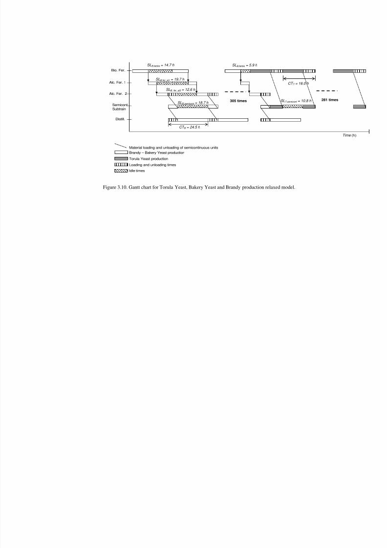
8/7/2019 Corsano G. Montagna J.M. Iribarren O.A. Aguirre P.A. Mathematical Modeling Approaches for Optimization of Chemic…
http://slidepdf.com/reader/full/corsano-g-montagna-jm-iribarren-oa-aguirre-pa-mathematical-modeling 67/103
Distill.
SemicontSubtrain
Alc. Fer. 2
Alc. Fer. 1
Bio. Fer.
305 times 281
CT T = 16.0 h
CT B = 24.5 h
SLB,ferbio = 14.7 h
SLB,fer_al1 = 19.7 h
SLB, fer_al2 = 12.6 h
SLB,semicont = 18.7 h SLT,semicont = 10.8 h
SLB,ferbio = 5.9 h
Idle times
Brandy – Bakery Yeast production
Torula Yeast production
Loading and unloading times
Material loading and unloading of semicontinuous units
Figure 3.10. Gantt chart for Torula Yeast, Bakery Yeast and Brandy production relaxed model.
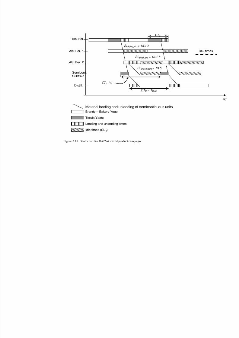
8/7/2019 Corsano G. Montagna J.M. Iribarren O.A. Aguirre P.A. Mathematical Modeling Approaches for Optimization of Chemic…
http://slidepdf.com/reader/full/corsano-g-montagna-jm-iribarren-oa-aguirre-pa-mathematical-modeling 68/103
Distill.
Semicont.Subtrain
Alc. Fer. 2
Alc. Fer. 1
Bio. Fer
CT B = T B,dis
CT T
SLB,semicont = 13 h
SLB,fer_al 2 = 13.1 h
SLB,fer_al 1 = 13.1 h
j CT j ∀
34
Brandy – Bakery Yeast
Torula Yeast
Loading and unloading times
Idle times (SLi j)
Material loading and unloading of semicontinuous units
Figure 3.11. Gantt chart for B-T/T-B mixed product campaign.
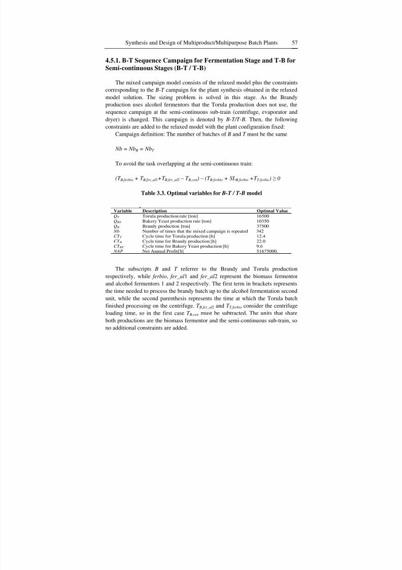
8/7/2019 Corsano G. Montagna J.M. Iribarren O.A. Aguirre P.A. Mathematical Modeling Approaches for Optimization of Chemic…
http://slidepdf.com/reader/full/corsano-g-montagna-jm-iribarren-oa-aguirre-pa-mathematical-modeling 69/103
Synthesis and Design of Multiproduct/Multipurpose Batch Plants 57
4.5.1. B-T Sequence Campaign for Fermentation Stage and T-B forSemi-continuous Stages (B-T / T-B)
The mixed campaign model consists of the relaxed model plus the constraints
corresponding to the B-T campaign for the plant synthesis obtained in the relaxed
model solution. The sizing problem is solved in this stage. As the Brandy
production uses alcohol fermentors that the Torula production does not use, the
sequence campaign at the semi-continuous sub-train (centrifuge, evaporator and
dryer) is changed. This campaign is denoted by B-T/T-B. Then, the following
constraints are added to the relaxed model with the plant configuration fixed:
Campaign definition: The number of batches of B and T must be the same
Nb = NbB = NbT
To avoid the task overlapping at the semi-continuous train:
(T B,ferbio + T B,fer_al1+T B,fer_al2 – T B,cen) – (T B,ferbio + SLB,ferbio +T T,ferbio) ≥ 0
Table 3.3. Optimal variables for B-T / T-B model
Variable Description Optimal Value
QT Torula production rate [ton] 16500QBY Bakery Yeast production rate [ton] 10350QB Brandy production [ton] 37500Nb Number of times that the mixed campaign is repeated 342CT T Cycle time for Torula production [h] 12.4CT B Cycle time for Brandy production [h] 22.0CT BY Cycle time for Bakery Yeast production [h] 9.6NAP Net Annual Profit[$] 51675000.
The subscripts B and T referrer to the Brandy and Torula production
respectively, while ferbio, fer_al1 and fer_al2 represent the biomass fermentor
and alcohol fermentors 1 and 2 respectively. The first term in brackets represents
the time needed to process the brandy batch up to the alcohol fermentation second
unit, while the second parenthesis represents the time at which the Torula batchfinished processing on the centrifuge. T B,fer_al2 and T T,ferbio consider the centrifuge
loading time, so in the first case T B,cen must be subtracted. The units that share
both productions are the biomass fermentor and the semi-continuous sub-train, so
no additional constraints are added.
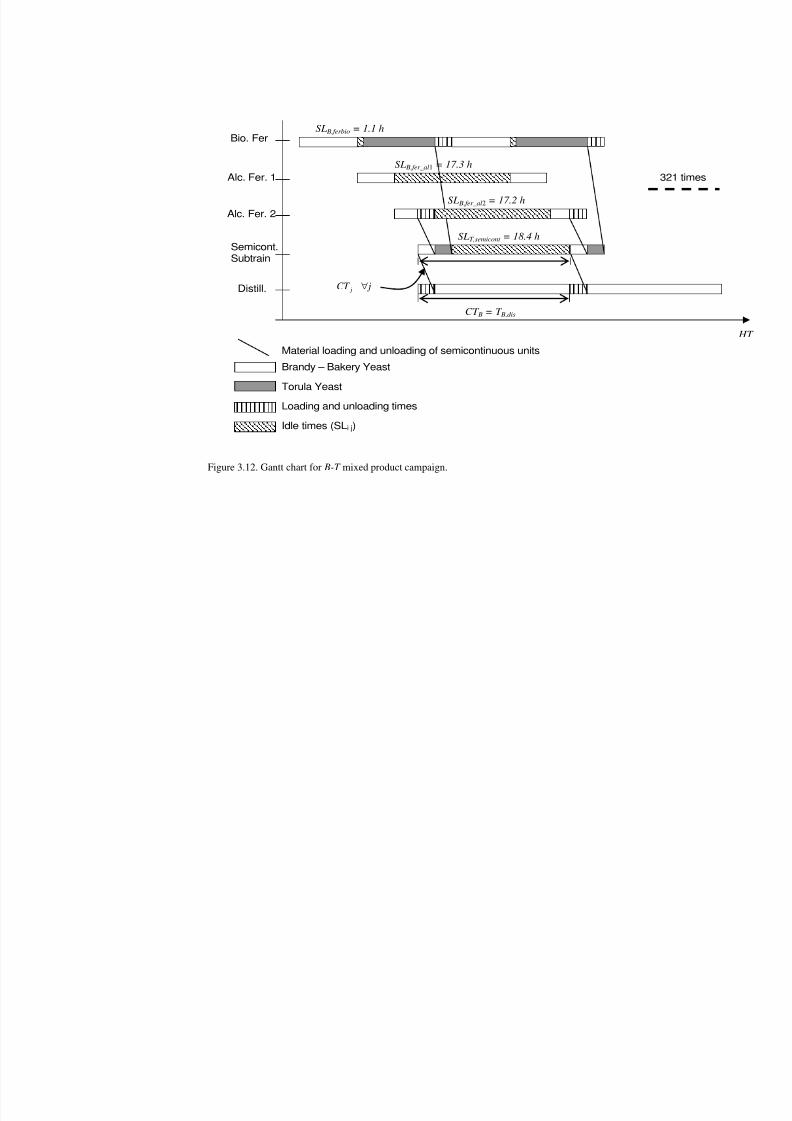
8/7/2019 Corsano G. Montagna J.M. Iribarren O.A. Aguirre P.A. Mathematical Modeling Approaches for Optimization of Chemic…
http://slidepdf.com/reader/full/corsano-g-montagna-jm-iribarren-oa-aguirre-pa-mathematical-modeling 70/103
Alc. Fer. 2
Distill.
Semicont.Subtrain
Alc. Fer. 1
Bio. Fer
CT B = T B,dis
Brandy – Bakery Yeast
Torula Yeast
Loading and unloading times
Idle times (SLi j)
SLB,fer_al1 = 17.3 h
j CT j
∀
32
SLB,fer_al2 = 17.2 h
SLT,semicont = 18.4 h
SLB,ferbio = 1.1 h
Material loading and unloading of semicontinuous units
Figure 3.12. Gantt chart for B-T mixed product campaign.
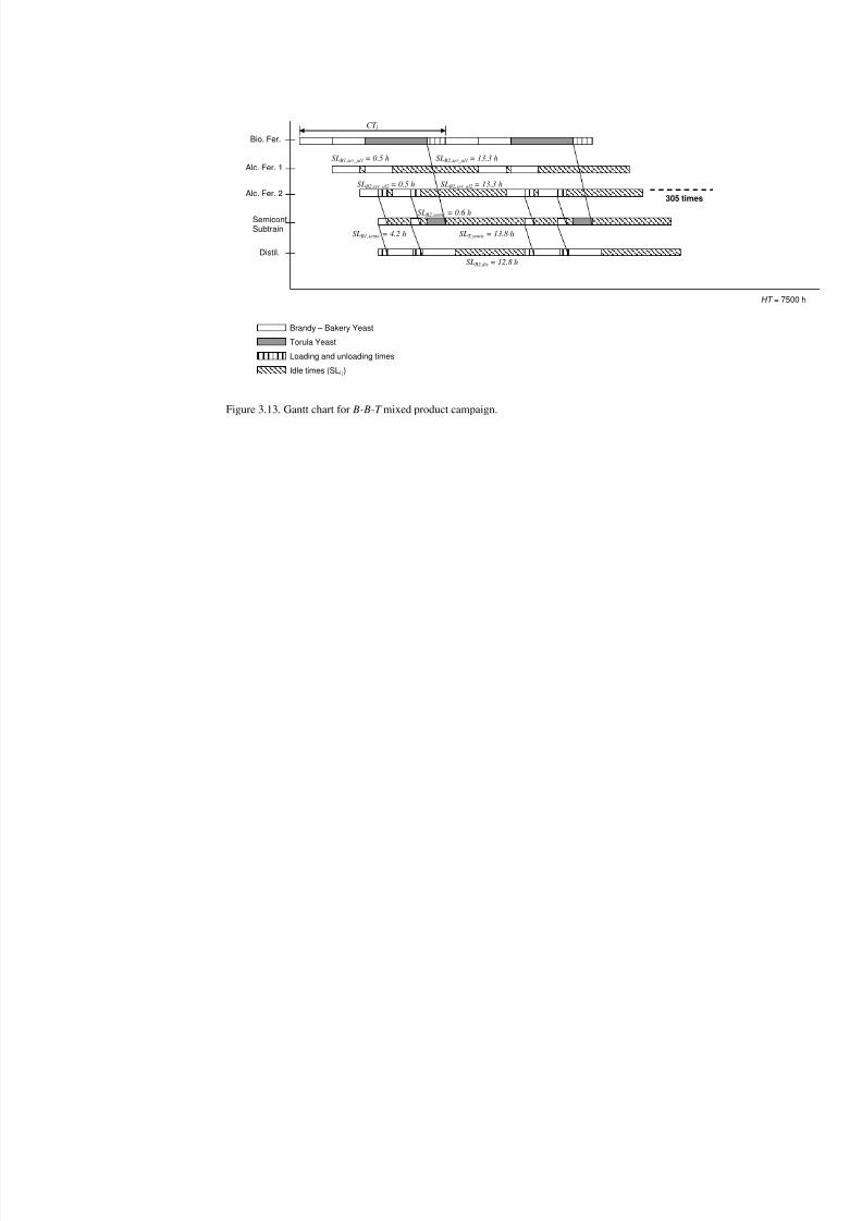
8/7/2019 Corsano G. Montagna J.M. Iribarren O.A. Aguirre P.A. Mathematical Modeling Approaches for Optimization of Chemic…
http://slidepdf.com/reader/full/corsano-g-montagna-jm-iribarren-oa-aguirre-pa-mathematical-modeling 71/103
Distil.
SemicontSubtrain
Alc. Fer. 2
Alc. Fer. 1
Bio. Fer.
Brandy – Bakery Yeast
Torula Yeast
Loading and unloading times
Idle times (SLi j)
305 times
CT j
SLB2,dis = 12.8 h
SLT,semic = 13.8 h
SLB2,ser_al2 = 13.3 h
SLB2,ser_al1 = 13.3 h
SLB1,semic = 4.2 h
SLB2,semic = 0.6 h
SLB1,ser_al1 = 0.5 h
SLB2,ser_al2 = 0.5 h
Figure 3.13. Gantt chart for B-B-T mixed product campaign.
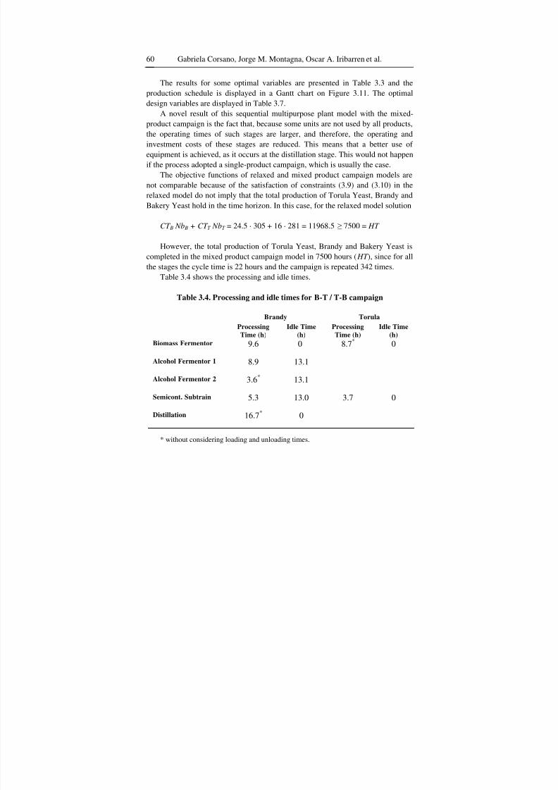
8/7/2019 Corsano G. Montagna J.M. Iribarren O.A. Aguirre P.A. Mathematical Modeling Approaches for Optimization of Chemic…
http://slidepdf.com/reader/full/corsano-g-montagna-jm-iribarren-oa-aguirre-pa-mathematical-modeling 72/103
Gabriela Corsano, Jorge M. Montagna, Oscar A. Iribarren et al.60
The results for some optimal variables are presented in Table 3.3 and the
production schedule is displayed in a Gantt chart on Figure 3.11. The optimal
design variables are displayed in Table 3.7.A novel result of this sequential multipurpose plant model with the mixed-
product campaign is the fact that, because some units are not used by all products,
the operating times of such stages are larger, and therefore, the operating and
investment costs of these stages are reduced. This means that a better use of
equipment is achieved, as it occurs at the distillation stage. This would not happen
if the process adopted a single-product campaign, which is usually the case.
The objective functions of relaxed and mixed product campaign models are
not comparable because of the satisfaction of constraints (3.9) and (3.10) in the
relaxed model do not imply that the total production of Torula Yeast, Brandy and
Bakery Yeast hold in the time horizon. In this case, for the relaxed model solution
CT B NbB + CT T NbT = 24.5 · 305 + 16 · 281 = 11968.5 ≥ 7500 = HT
However, the total production of Torula Yeast, Brandy and Bakery Yeast is
completed in the mixed product campaign model in 7500 hours (HT ), since for all
the stages the cycle time is 22 hours and the campaign is repeated 342 times.
Table 3.4 shows the processing and idle times.
Table 3.4. Processing and idle times for B-T / T-B campaign
Brandy Torula
Processing
Time (h)
Idle Time
(h)
Processing
Time (h)
Idle Time
(h)
Biomass Fermentor 9.6 0 8.7* 0
Alcohol Fermentor 1 8.9 13.1
Alcohol Fermentor 2 3.6* 13.1
Semicont. Subtrain 5.3 13.0 3.7 0
Distillation 16.7* 0
* without considering loading and unloading times.
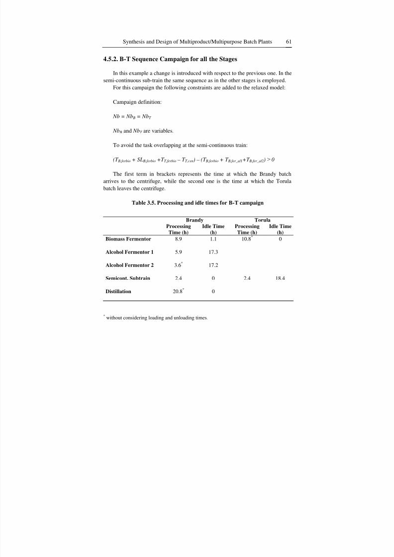
8/7/2019 Corsano G. Montagna J.M. Iribarren O.A. Aguirre P.A. Mathematical Modeling Approaches for Optimization of Chemic…
http://slidepdf.com/reader/full/corsano-g-montagna-jm-iribarren-oa-aguirre-pa-mathematical-modeling 73/103
Synthesis and Design of Multiproduct/Multipurpose Batch Plants 61
4.5.2. B-T Sequence Campaign for all the Stages
In this example a change is introduced with respect to the previous one. In thesemi-continuous sub-train the same sequence as in the other stages is employed.
For this campaign the following constraints are added to the relaxed model:
Campaign definition:
Nb = NbB = NbT
NbB and NbT are variables.
To avoid the task overlapping at the semi-continuous train:
(T B,ferbio + SLB,ferbio +T T,ferbio – T T,cen) – (T B,ferbio + T B,fer_al1+T B,fer_al2) ≥ 0
The first term in brackets represents the time at which the Brandy batch
arrives to the centrifuge, while the second one is the time at which the Torula
batch leaves the centrifuge.
Table 3.5. Processing and idle times for B-T campaign
Brandy TorulaProcessing
Time (h)
Idle Time
(h)
Processing
Time (h)
Idle Time
(h)
Biomass Fermentor 8.9
1.1 10.8*
0
Alcohol Fermentor 1 5.9 17.3
Alcohol Fermentor 2 3.6*
17.2
Semicont. Subtrain 2.4 0 2.4 18.4
Distillation 20.8*
0
* without considering loading and unloading times.
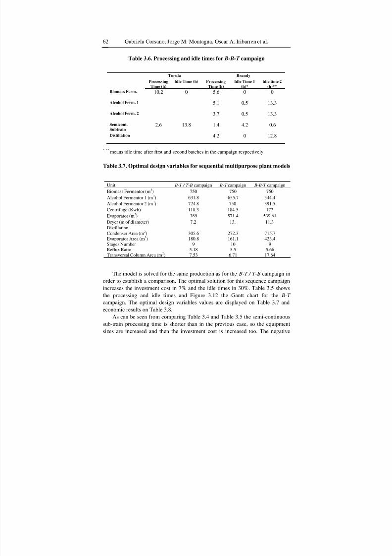
8/7/2019 Corsano G. Montagna J.M. Iribarren O.A. Aguirre P.A. Mathematical Modeling Approaches for Optimization of Chemic…
http://slidepdf.com/reader/full/corsano-g-montagna-jm-iribarren-oa-aguirre-pa-mathematical-modeling 74/103
Gabriela Corsano, Jorge M. Montagna, Oscar A. Iribarren et al.62
Table 3.6. Processing and idle times for B-B-T campaign
Torula Brandy
Processing
Time (h)
Idle Time (h) Processing
Time (h)
Idle Time 1
(h)*
Idle time 2
(h)**
Biomass Ferm. 10.2 0 5.6 0 0
Alcohol Ferm. 1 5.1 0.5 13.3
Alcohol Ferm. 2 3.7 0.5 13.3
Semicont.
Subtrain2.6 13.8 1.4 4.2 0.6
Distillation 4.2 0 12.8
*, ** means idle time after first and second batches in the campaign respectively
Table 3.7. Optimal design variables for sequential multipurpose plant models
Unit B-T / T-B campaign B-T campaign B-B-T campaign
Biomass Fermentor (m3) 750 750 750
Alcohol Fermentor 1 (m3) 631.8 655.7 344.4
Alcohol Fermentor 2 (m3) 724.8 750 391.5
Centrifuge (Kwh) 118.3 184.5 172
Evaporator (m2) 389 571.4 539.61
Dryer (m of diameter) 7.2 13. 11.3
DistillationCondenser Area (m2)Evaporator Area (m2)Stages NumberReflux RatioTransversal Column Area (m2)
305.6180.8
95.187.53
272.3161.1
105.5
6.71
715.7423.4
95.6617.64
The model is solved for the same production as for the B-T / T-B campaign in
order to establish a comparison. The optimal solution for this sequence campaign
increases the investment cost in 7% and the idle times in 30%. Table 3.5 shows
the processing and idle times and Figure 3.12 the Gantt chart for the B-T
campaign. The optimal design variables values are displayed on Table 3.7 and
economic results on Table 3.8.
As can be seen from comparing Table 3.4 and Table 3.5 the semi-continuous
sub-train processing time is shorter than in the previous case, so the equipment
sizes are increased and then the investment cost is increased too. The negative
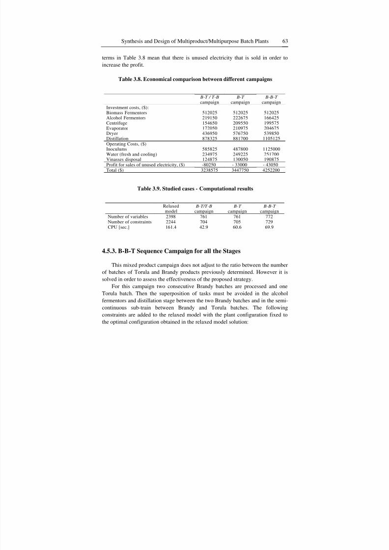
8/7/2019 Corsano G. Montagna J.M. Iribarren O.A. Aguirre P.A. Mathematical Modeling Approaches for Optimization of Chemic…
http://slidepdf.com/reader/full/corsano-g-montagna-jm-iribarren-oa-aguirre-pa-mathematical-modeling 75/103
Synthesis and Design of Multiproduct/Multipurpose Batch Plants 63
terms in Table 3.8 mean that there is unused electricity that is sold in order to
increase the profit.
Table 3.8. Economical comparison between different campaigns
B-T / T-B campaign
B-T
campaignB-B-T
campaignInvestment costs, ($):Biomass FermentorsAlcohol FermentorsCentrifugeEvaporatorDryerDistillation
512025219150154650172050436950878325
512025222675209550210975576750881700
512025166425199575204675539850
1105125
Operating Costs, ($)InoculumsWater (fresh and cooling)Vinasses disposal
585825234975124875
487800249225130050
1125000251700190875
Profit for sales of unused electricity, ($) -80250 - 33000 - 43050Total ($) 3238575 3447750 4252200
Table 3.9. Studied cases - Computational results
Relaxedmodel
B-T/T-B campaign
B-T campaign
B-B-T campaign
Number of variables 2398 761 761 772Number of constraints 2244 704 705 729CPU [sec.] 161.4 42.9 60.6 69.9
4.5.3. B-B-T Sequence Campaign for all the Stages
This mixed product campaign does not adjust to the ratio between the number
of batches of Torula and Brandy products previously determined. However it is
solved in order to assess the effectiveness of the proposed strategy.
For this campaign two consecutive Brandy batches are processed and oneTorula batch. Then the superposition of tasks must be avoided in the alcohol
fermentors and distillation stage between the two Brandy batches and in the semi-
continuous sub-train between Brandy and Torula batches. The following
constraints are added to the relaxed model with the plant configuration fixed to
the optimal configuration obtained in the relaxed model solution:
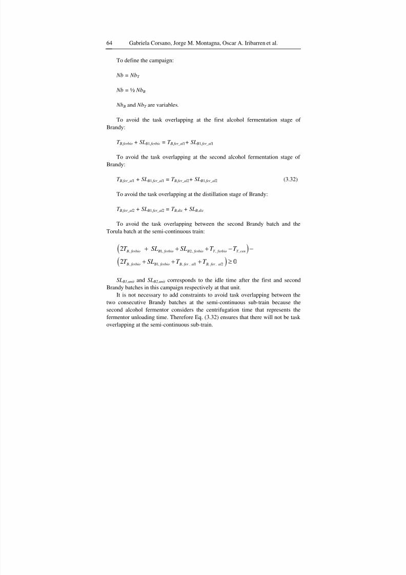
8/7/2019 Corsano G. Montagna J.M. Iribarren O.A. Aguirre P.A. Mathematical Modeling Approaches for Optimization of Chemic…
http://slidepdf.com/reader/full/corsano-g-montagna-jm-iribarren-oa-aguirre-pa-mathematical-modeling 76/103
Gabriela Corsano, Jorge M. Montagna, Oscar A. Iribarren et al.64
To define the campaign:
Nb = NbT
Nb = ½ NbB
NbB and NbT are variables.
To avoid the task overlapping at the first alcohol fermentation stage of
Brandy:
T B,ferbio + SLB1,ferbio = T B,fer_al1+ SLB1,fer_al1
To avoid the task overlapping at the second alcohol fermentation stage of
Brandy:
T B,fer_al1 + SLB1,fer_al1 = T B,fer_al2+ SLB1,fer_al2 (3.32)
To avoid the task overlapping at the distillation stage of Brandy:
T B,fer_al2 + SLB1,fer_al2 = T B,dis + SLB,dis
To avoid the task overlapping between the second Brandy batch and theTorula batch at the semi-continuous train:
( )
( ), 1, 2, , ,
, 1, , _ 1 , _ 2
2
2 0
B ferbio B ferbio B ferbio T ferbio T cen
B ferbio B ferbio B fer al B fer al
T SL SL T T
T SL T T
+ + + − −
+ + + ≥
SLB1,unit and SLB2,unit corresponds to the idle time after the first and second
Brandy batches in this campaign respectively at that unit.
It is not necessary to add constraints to avoid task overlapping between the
two consecutive Brandy batches at the semi-continuous sub-train because thesecond alcohol fermentor considers the centrifugation time that represents the
fermentor unloading time. Therefore Eq. (3.32) ensures that there will not be task
overlapping at the semi-continuous sub-train.
8/7/2019 Corsano G. Montagna J.M. Iribarren O.A. Aguirre P.A. Mathematical Modeling Approaches for Optimization of Chemic…
http://slidepdf.com/reader/full/corsano-g-montagna-jm-iribarren-oa-aguirre-pa-mathematical-modeling 77/103
Synthesis and Design of Multiproduct/Multipurpose Batch Plants 65
For the B-B-T campaign, the optimal solution is about a 31% worse than the
objective function obtained in example 3.5.1 for the same production. Table 3.6
shows the processing and idle times for this campaign. As can be observed, thedistillation processing time is reduced more than three times, so the investment
cost is also incremented (Table 3.8). The unit sizes for this campaign can be
observed on Table 3.7. The total idle time is increased in 26%. Figure 3.13 shows
the Gantt chart for this example.
As the earnings from sales are the same in all cases since the productions are
fixed, Table 3.8 compares the investment and operation costs of the first campaign
analyzed and this last campaign. In both cases, there is unused electricity that is
considered as benefit.
Another disadvantage of this campaign is that the biomass fermentor is sub-
occupied in Brandy production (Brandy batch size in biomass fermentor is 308.64m3, while the biomass fermentor size is 750 m3 because it reaches this value for
Torula production). This occurs because the same production that was first
reached in one batch is now reached after two batches.
Only the alcohol fermentation stage is cheaper in this case because the unit
sizes are smaller. This occurs because each Brandy batch size is smaller since two
batches are processed.
Table 3.7 shows the unit sizes for the different examples studied.
Table 3.9 presents the solutions times and number of variables and constraints
of each studied case. The reduction of the number of variables and constraints in
mixed product campaign models is because these models the plant configurationis fixed and therefore the superstructure model is not considered.
4.6. CONCLUSIONS AND OUTLOOK ON THE PROPOSED
HEURISTIC APPROACH FOR MIXED PRODUCT CAMPAIGN MODEL
In this book section a detailed model for the optimal synthesis, design,
operation and scheduling of a sequential multipurpose non-continuous plant was
developed. The resolution strategy considers two steps. Firstly, a relaxed model is
solved to obtain the number of batches of each product and the plant synthesis.
Then the designer chooses the mixed campaign based on the ratio between the
number of batches. A novel set of tasks scheduling constraints was proposed in
order to avoid tasks superposition at processing units.
8/7/2019 Corsano G. Montagna J.M. Iribarren O.A. Aguirre P.A. Mathematical Modeling Approaches for Optimization of Chemic…
http://slidepdf.com/reader/full/corsano-g-montagna-jm-iribarren-oa-aguirre-pa-mathematical-modeling 78/103
Gabriela Corsano, Jorge M. Montagna, Oscar A. Iribarren et al.66
The problem was formulated as an NLP model and a superstructure model
presented in section 2 was embedded in order to solve the synthesis problem.
There are not previous published works dealing with the synthesis, design andscheduling problem simultaneously solved as an NLP model.
Another characteristic of these models is the high level of detail reached in
the processing unit description, some of them by means of ordinary differentials
equations. Batch blending, batch splitting and recycles are allowed as novel
components for the multipurpose plant model, decisions taken in this work as
optimization variables.
The model was implemented for a Torula Yeast, Brandy and Bakery Yeast
production plant. The model was formulated and solved according to the proposed
strategy. The optimal solution was compared with different campaign sequences.
In all the cases, the investment and operative costs and the idle times wereincreased. Economic as well as synthesis, design and operational results are also
reported. The gap between the objective function value of the relaxed model
solution and the objective value of the mixed product campaign model is very
tight, which ensures that the solution obtained for the mixed product campaign is
the optimal and serves to validate the proposed heuristic methodology.
8/7/2019 Corsano G. Montagna J.M. Iribarren O.A. Aguirre P.A. Mathematical Modeling Approaches for Optimization of Chemic…
http://slidepdf.com/reader/full/corsano-g-montagna-jm-iribarren-oa-aguirre-pa-mathematical-modeling 79/103
Chapter 5
PROCESS INTEGRATION:MATHEMATICAL MODELING FOR THE
OPTIMAL SYNTHESIS, DESIGN, OPERATION
AND PLANNING OF A MULTIPLANT COMPLEX
5.1. INTRODUCTION
The constant shift towards production of higher-added value products in
chemical processing industries has encouraged modeling and optimization studies
of batch processes. Whereas significant development has been made in designing,
planning and scheduling of batch plants with single or multiple production routes,the problem of synthesis, design, operation, and planning in batch multiplant
complexes has received much less attention.
In a multiplant complex (MC), there are two or more interconnected plants
that are supplied with raw materials and energy by a mother plant and by external
plants. The mother plant produces raw materials and energy resources r (r = 1, …,
N r ) that are considered as “produced resources”. The derivative plants l (l = 1, …,
L) can also receive resources from other not nearby plants (external plants). This
type of resources is called “supplied resources”. The unused resources, those
produced by the mother plant and not used in the derivative plants, can be sold
and they are called “exported resources”.The MC considered in this work includes plants that can produce only one
product and the production of a by-product is allowed. A by-product is a product
which is obtained by splitting a batch or processing it in a different manner.
The derivative plants have batch and semi-continuous units, and mixing,
splitting, and recycling batches are allowed. The residue of a derivative plant may
become raw material of the same plant or of another derivative plant. If the
8/7/2019 Corsano G. Montagna J.M. Iribarren O.A. Aguirre P.A. Mathematical Modeling Approaches for Optimization of Chemic…
http://slidepdf.com/reader/full/corsano-g-montagna-jm-iribarren-oa-aguirre-pa-mathematical-modeling 80/103
Gabriela Corsano, Jorge M. Montagna, Oscar A. Iribarren et al.68
residue is discarded, a disposal cost is allocated. Recycles amount and
concentration are process variables and the allocation or not of a recycled flow to
processing unit is also an optimization variable.In this section a detailed NLP model is developed in order to obtain the
optimal synthesis, design, and operation of a MC. The structure of the plant is
decided on simultaneously with the design, operating, and scheduling issues. The
objective function employed is the maximization of annualized net profit given by
the total expected sales price minus the total investment and operation cost, as was
presented in the previous section.
The work is focused on providing a tool for generating and evaluating
different alternatives of product production. The importance of this approach lies
in the integration of synthesis, design, operation, and scheduling decisions
working on a multiplant complex where trade-offs must be contemplated amongthe different processes. When simultaneously approached, these decisions allow
considering the relationships and effects between critical elements of the problem
that are usually analyzed sequentially.
The example in Figure 1.2 shows that with only two derivative plants, there
are interconnections between the derivative plants given by residue recycles and
intermediate productions. In our approach, both derivative plants can produce a
product and a by-product. Besides producing material and energy resources for
derivative plants, the mother plant produces final products to be sold.
The synthesis, design and operation problem for multiplant complex
production is defined as follows:Given N p derivative products to be processed, their production targets, selling
prices, and the production routes for each product, determine the plant
configuration for each product including unit sizes, material and energy streams
among the plants and the involved processing variables in order to obtain the best
economical and environmental solution.
5.2. MODEL FORMULATION
In a MC, each product is produced in a different plant and some plants canalso produce by-products. Given N p different derivative products and by-products
to be processed in L different plants, the model considers:
Mass balances at every unit of each plant: some of them are given by
differential equations which are discretized and included in the global model as
algebraic equations, for example
8/7/2019 Corsano G. Montagna J.M. Iribarren O.A. Aguirre P.A. Mathematical Modeling Approaches for Optimization of Chemic…
http://slidepdf.com/reader/full/corsano-g-montagna-jm-iribarren-oa-aguirre-pa-mathematical-modeling 81/103
Process Integration 69
( , ) 1,..., , 1, .., ,xlj
x l
dC h t x x N l L j E
dt = = = ∈ (4.1)
where C xlj is the concentration of component x (biomass, substrate, product, etc.),
at stage j of plant l. E l represents the set of units of plant l. These dynamic
equations are discretized and included in the overall model as algebraic equations
in the same way as it was posed in the previous section.
Mass balances between units of the same plant:
, 1
1
1,.., ,r N
lj ljr l j l
r
VS F VS l L j E −=
= + ∀ = ∀ ∈∑ (4.2)
, 1 , 11
1,.., ,r N
ini r fin
lj xlj xlj ljr xl j l j l
r
VS C C F C VS l L j E − −=
= + ∀ = ∀ ∈∑ (4.3)
where superscripts ini and fin represent the initial and final concentration
respectively and VSlj represents the batch volume at stage j in plant l, and F ljr is
the amount of resource r used in unit j at plant l.
Interconnection constraints between the mother plant and derivative plants:
The material and energy required resources for each process production can
be obtained from the mother plant (prod
r F ) or can be supplied for another plant
outside the complex ( s
r F ). The unused amount of resource r , i.e. the amount of r
that is not consumed by the derivative plants (ex
r F ), can be sold to market. The
constraints for the consumed resources are:
1 1
lN Lrljprod s ex
r r r
l j l
f F F F
CT = =
+ = +∑∑ for each resource r (4.4)
where f rlj is the amount of r consumed at stage j in the derivative plant l. CT l
represents the cycle time of plant l defined by
CT lt ≥ T j , 1, ...,l
j E l L∈ = (4.5)
8/7/2019 Corsano G. Montagna J.M. Iribarren O.A. Aguirre P.A. Mathematical Modeling Approaches for Optimization of Chemic…
http://slidepdf.com/reader/full/corsano-g-montagna-jm-iribarren-oa-aguirre-pa-mathematical-modeling 82/103
Gabriela Corsano, Jorge M. Montagna, Oscar A. Iribarren et al.70
where T j is the time for processing a batch at stage j of plant l in time period t . Let
k θ be the processing time at semi-continuous stage k of plant l, then
' '' , ', ''j k j k l
T t for j k k E θ θ = + + ∈ (4.6)
Note that Eq. (4.6) defines the time that unit j will be occupied is the
processing time of the batch (t j), plus the material loading ( 'k θ ) and unloading
( ''k θ ) time if this unit is located between semi-continuous units. It is worth noting
that in this approach it is assumed that variables t j andk
θ are involved in detailed
sub-models some of them written as differential equations and included in the
actual model (Corsano et al., 2004).If a product and a by-product are produced in a plant l, then CT l defined as
(4.5) is the maximum of all processing time of units j used for the production of
the product and by-product.
All products must be produced within the production time horizon. In this
work, the time horizon is the same for all plants (HT ); so:
Nbl CT l ≤ HT for each l = 1, …, L (4.7)
If a product and a by-product are produced in plant l, then
Nbi CT l ≤ HT for each i product produced in plant l = 1, …, L (4.7’)
The interconnection constraints between derivative plants: mass and energy
balances and the recycle equations between two different plants and/or from one
stage to another in the same production process.
e e
e e
lj lj
l L j EB
F f e∈ ∈
≥ ∀∑ ∑ (4.8)
where eljF is the amount of recycle e produced at stage j in plant l, and e
ljf is the
amount of recycle e consumed at stage j in plant l. Le and EBe represent the set of
plants and units that consume e respectively. For model simplification purposes,
the store cost of raw materials and effluents is not considered in this work.
8/7/2019 Corsano G. Montagna J.M. Iribarren O.A. Aguirre P.A. Mathematical Modeling Approaches for Optimization of Chemic…
http://slidepdf.com/reader/full/corsano-g-montagna-jm-iribarren-oa-aguirre-pa-mathematical-modeling 83/103
Process Integration 71
The design equations for each batch and semi-continuous unit depend on
process variables as follows:
produced in , , 1,..,l
lj ij i lV S B i l j E l L≥ ∀ ∀ ∈ ∀ = (4.9)
produced in , , 1,..,l ilk ik l
ik
BV S i l k E l L
θ ≥ ∀ ∀ ∈ ∀ = (4.10)
where S represents size or duty factor of batch and semi-continuous units
respectively. These factors are computed as a function of the process variables. In
the last two equations, product i and plant l appear simultaneously because of
some plants can produce a by-product, and thus they manufacture more than oneproduct. Bi is the batch size of product i, and V lj and V lk are the batch and semi-
continuous unit size respectively.
The production constraints of each plant:
For each product i produced in plant l, the required demand has to be satisfied
produced in , 1,..,i i i
B Nb Q i l l L= ∀ ∀ = (4.11)
min max i i i
Q Q Q≤ ≤ (4.12)
where Qi is the production of product i which is bounded bymin
iQ andmax
iQ .
Just like in the multipurpose plant model, a superstructure model that
considers a set of different alternatives configurations is embedded in the overall
model so that the model keeps the NLP nature.
The objective function: the maximization of annualized net profits given by
the total expected total sales minus the investment and operative costs:
( )'
1 1 1 1
Resp r r
lj lk
l l
N N N Lex imp prod
i i r r lj lj lk lk l r r r r
i r l j E k E r
Max pQ HT q F V V HT c F c F β β
α α
= = = ∈ ∈ =
⎛ ⎞⎛ ⎞+ − + + + +⎜ ⎟⎜ ⎟⎜ ⎟
⎝ ⎠⎝ ⎠
∑ ∑ ∑ ∑ ∑ ∑
(4.13)
where Resl represents the disposal cost for each plant l, pi and qr are the selling
price of product i and resource r respectively, while cr and'
r c are the imported
and produced resource costs respectively.
8/7/2019 Corsano G. Montagna J.M. Iribarren O.A. Aguirre P.A. Mathematical Modeling Approaches for Optimization of Chemic…
http://slidepdf.com/reader/full/corsano-g-montagna-jm-iribarren-oa-aguirre-pa-mathematical-modeling 84/103
Gabriela Corsano, Jorge M. Montagna, Oscar A. Iribarren et al.72
The MC model considers constraints (4.1)-(4.13), which are simultaneously
optimized and no heuristic or decomposition strategy is applied.
5.3. MULTIPLANT COMPLEX TO PRODUCE DERIVATIVES
FROM SUGAR CANE
The Cane Sugar Complex consists of three plants interconnected by material
and energy flows. The plants that constitute the complex are a Sugar plant (mother
plant) and two derivative plants: Torula Yeast and Brandy/Bakery Yeast.
Production processes were described in Section 3.5, with the only difference
that in this scenario each product is manufactured in a different plant. Bakery
Yeast is a by-product of Brandy plant.
For both derivative plants, the configuration of the fermentation stage is
obtained using the superstructure model presented in Section 2 of this chapter
embedded in the global integration model, considering only in series units
duplication.
The derivatives plants are connected by the vinasses recycles, and the
connections between Sugar and derivatives plants are given by material (molasses
and filter juices) and energy (vapor and electricity) resources.
For the vinasses recycle equation (4.8) is rewritten as:
{ } { }, , ,
DV DV DV
brandy dist brandy brandy torula j torula brandy j brandy
j fermentors j fermentors
F Nb Res f Nb f Nb∈ ∈
+ = +∑ ∑
where DV means distillery vinasses and Resbrandy represent the residual vinasses.
For the electricity integration between the mother plant and derivative plants,
for instance, equation (4.4) is rewritten as
, , , ,
prod s ex
elec elec torula cent elec brany centr elec elecF F F F F + = + +
where cent means centrifuge, the only stage that consumes electricity.
In Table 4.1 the different simultaneous decisions made in this model are
described.
Figure 4.1 shows the Sugar Complex integration. This figure shows that the
model considers blending, recycling and splitting batches.
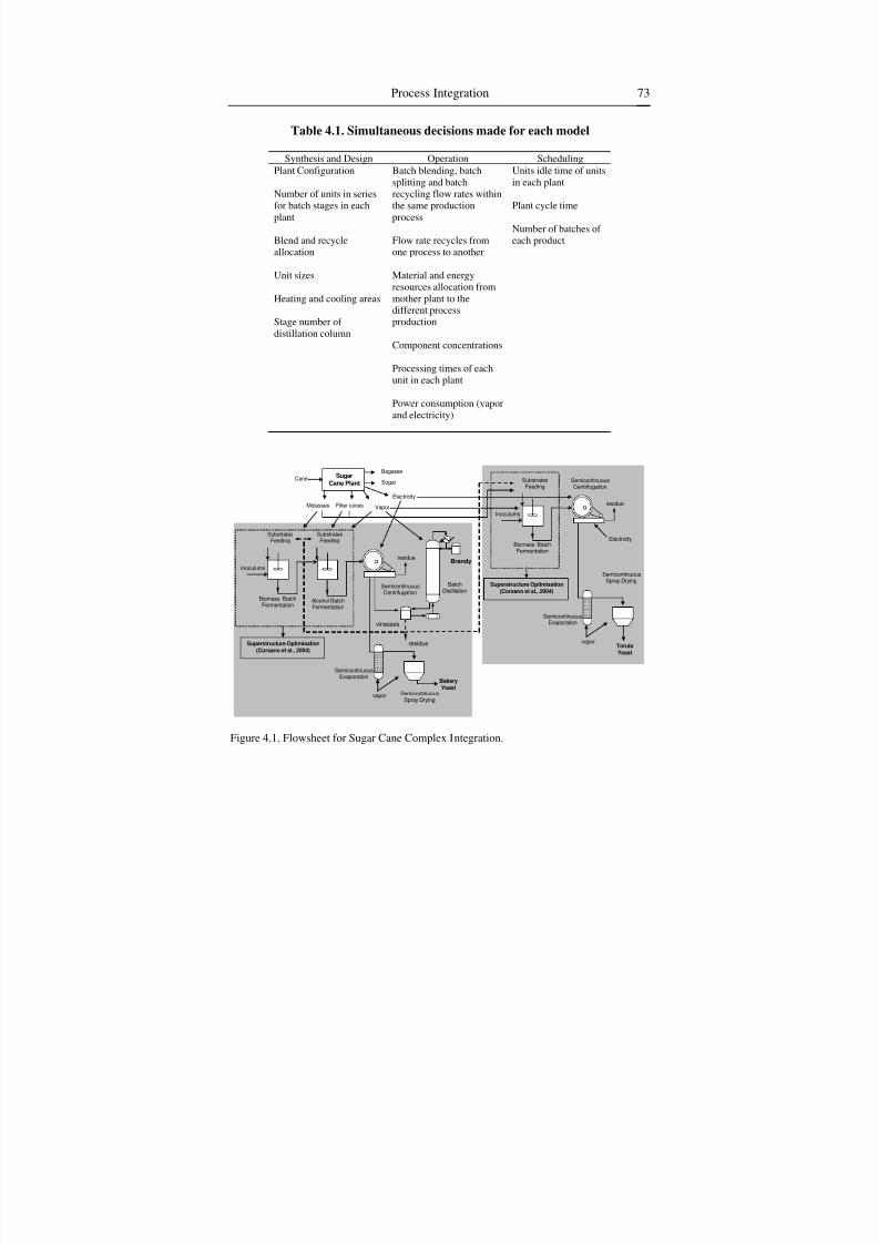
8/7/2019 Corsano G. Montagna J.M. Iribarren O.A. Aguirre P.A. Mathematical Modeling Approaches for Optimization of Chemic…
http://slidepdf.com/reader/full/corsano-g-montagna-jm-iribarren-oa-aguirre-pa-mathematical-modeling 85/103
8/7/2019 Corsano G. Montagna J.M. Iribarren O.A. Aguirre P.A. Mathematical Modeling Approaches for Optimization of Chemic…
http://slidepdf.com/reader/full/corsano-g-montagna-jm-iribarren-oa-aguirre-pa-mathematical-modeling 86/103
Gabriela Corsano, Jorge M. Montagna, Oscar A. Iribarren et al.74
5.4. RESULTS AND ANALYSIS
The presented model for optimal synthesis, design, operation and scheduling
of MC provide a tool for the analysis of different alternative configurations. In
addition, the economical tradeoffs among the different contemplated elements can
be established and assessed. In this section, the results of the optimization of the
model under different operative conditions and their analysis are shown for the
Torula Yeast, Brandy and Bakery Yeast processes integrated to a Sugar plant as it
was presented in the previous section. This study is based on specific data of
product profits, equipment and resources costs, etc. These values can be modified
by the manager or the designer, taking into account different contexts or
scenarios. In particular, this work tries to show the advantages of considering all
these elements simultaneously so as to assess the effects or relationships betweenthem. Regardless of the attained results, which depend on several factors, the
analytic capability of this approach is emphasized.
Due to a matter of limited space, only one example is presented here. For
more examples and detailed analysis, review the work of Corsano et al. (2006c).
All models were implemented and solved in GAMS (Brooke et al., 1998) in a
Pentium IV, 1.60 Ghz. The code CONOPT2 was employed to solve the NLP
problems. The MC model has about 1100 equations 1200 variables, and CPU time
for its resolution is about 160 sec.
In this section, we show the optimal solution for the MC model with the same
model parameters employed in the previous section for Multiproduct Plant (MP)scenario. Then, taking into account the example analyzed in section 3, the both
scenarios are compared. Therefore, through two different models, two possible
production options are assessed and compared. Thus, we prove the versatility of
mathematical models in order to make decisions in different contexts. Not only
different options in a specific scenario can be evaluated, but also different
scenarios can be compared.
EXAMPLE
In order to evaluate different production alternatives, the MC model is solved
for the same operative condition presented for the case of multiproduct plant
model of Section 3, that is,min
iQ = 7500 ton and
max
iQ = 37500 ton for Torula and
Brandy production, while for Bakery Yeast production no bounds are imposed
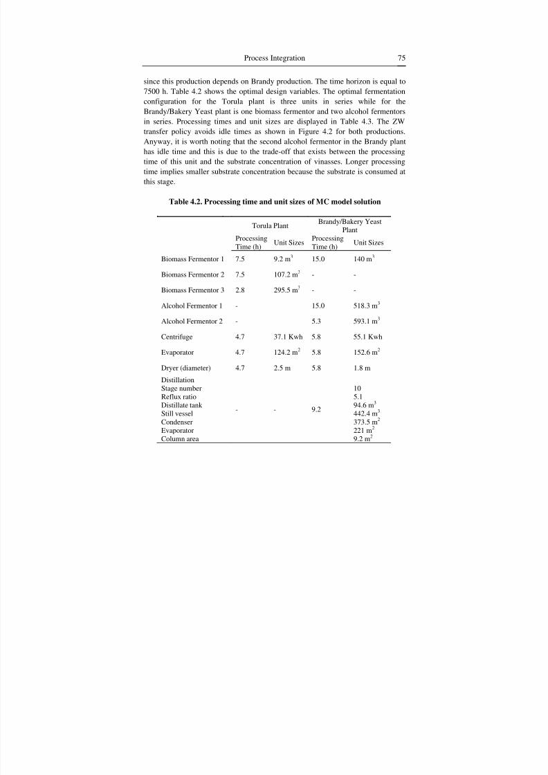
8/7/2019 Corsano G. Montagna J.M. Iribarren O.A. Aguirre P.A. Mathematical Modeling Approaches for Optimization of Chemic…
http://slidepdf.com/reader/full/corsano-g-montagna-jm-iribarren-oa-aguirre-pa-mathematical-modeling 87/103
Process Integration 75
since this production depends on Brandy production. The time horizon is equal to
7500 h. Table 4.2 shows the optimal design variables. The optimal fermentation
configuration for the Torula plant is three units in series while for theBrandy/Bakery Yeast plant is one biomass fermentor and two alcohol fermentors
in series. Processing times and unit sizes are displayed in Table 4.3. The ZW
transfer policy avoids idle times as shown in Figure 4.2 for both productions.
Anyway, it is worth noting that the second alcohol fermentor in the Brandy plant
has idle time and this is due to the trade-off that exists between the processing
time of this unit and the substrate concentration of vinasses. Longer processing
time implies smaller substrate concentration because the substrate is consumed at
this stage.
Table 4.2. Processing time and unit sizes of MC model solution
Torula PlantBrandy/Bakery Yeast
PlantProcessingTime (h)
Unit SizesProcessingTime (h)
Unit Sizes
Biomass Fermentor 1 7.5 9.2 m3 15.0 140 m3
Biomass Fermentor 2 7.5 107.2 m3 - -
Biomass Fermentor 3 2.8 295.5 m3 - -
Alcohol Fermentor 1 - 15.0 518.3 m3
Alcohol Fermentor 2 - 5.3 593.1 m3
Centrifuge 4.7 37.1 Kwh 5.8 55.1 Kwh
Evaporator 4.7 124.2 m2 5.8 152.6 m2
Dryer (diameter) 4.7 2.5 m 5.8 1.8 m
DistillationStage numberReflux ratio
Distillate tank Still vesselCondenserEvaporatorColumn area
- - 9.2
105.1
94.6 m3
442.4 m3 373.5 m2 221 m2
9.2 m2
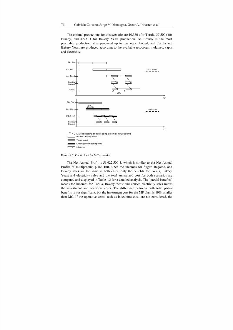
8/7/2019 Corsano G. Montagna J.M. Iribarren O.A. Aguirre P.A. Mathematical Modeling Approaches for Optimization of Chemic…
http://slidepdf.com/reader/full/corsano-g-montagna-jm-iribarren-oa-aguirre-pa-mathematical-modeling 88/103
Gabriela Corsano, Jorge M. Montagna, Oscar A. Iribarren et al.76
The optimal productions for this scenario are 10,350 t for Torula, 37,500 t for
Brandy, and 4,500 t for Bakery Yeast production. As Brandy is the most
profitable production, it is produced up to this upper bound; and Torula andBakery Yeast are produced according to the available resources: molasses, vapor
and electricity.
Distill.
Semicont.Subtrain
Alc. Fer. 2
Alc. Fer. 1
Bio. Fer
CT B
500 times
HT
Semicont.Subtrain
Bio. Fer. 3
Bio. Fer. 2
Bio. Fer 1
1000 times
HT
Brandy – Bakery Yeast
Torula Yeast
Loading and unloading times
Idle times
Material loading and unloading of semicontinuous units
CT T
Figure 4.2. Gantt chart for MC scenario.
The Net Annual Profit is 51,622,500 $, which is similar to the Net Annual
Profits of multiproduct plant. But, since the incomes for Sugar, Bagasse, and
Brandy sales are the same in both cases, only the benefits for Torula, Bakery
Yeast and electricity sales and the total annualized cost for both scenarios are
compared and displayed in Table 4.3 for a detailed analysis. The “partial benefits”
means the incomes for Torula, Bakery Yeast and unused electricity sales minus
the investment and operative costs. The difference between both total partial
benefits is not significant, but the investment cost for the MP plant is 19% smaller
than MC. If the operative costs, such as inoculums cost, are not considered, the
8/7/2019 Corsano G. Montagna J.M. Iribarren O.A. Aguirre P.A. Mathematical Modeling Approaches for Optimization of Chemic…
http://slidepdf.com/reader/full/corsano-g-montagna-jm-iribarren-oa-aguirre-pa-mathematical-modeling 89/103
Process Integration 77
optimal solution may change. In this case, the operative costs are higher for the
MP plant because productions are mutually dependent since all products are
produced in the same plant; while at MC plant scenario, processes performancesare good and there is an efficient use of units because each product is produced in
a separate plant. Therefore, it is very important to simultaneously consider all
these characteristics in order to perform a real comparison.
In addition, human resource demand is higher for the MC scenario than in MP
plant. If we assume that one worker is needed for the fermentation stages, one for
the semi-continuous units and one for the distillation stage, and considering three
work shifts a day, 9 workers will be needed for the MP plant against 15 for MC
plant. Human resources demand is not considered in the model.
Since each product is produced in a separate plant in MC scenario, each
process production is performed optimally under the integration conditionsbecause the units in each plant are exclusively used for only one product. The
biomass fermentation stage performance is better in MC because a good use of
units is achieved since there are no idle times and no underused units. The
investment cost for this stage is about 30% higher for the MC because the total
number of units used in this case is greater than in the MP scenario as a result of
production in separate plants. The same difference occurs for semi-continuous
units. It can be noted that the inoculums cost is lower for the MC plant due to the
good use of fermentative units. The investment cost of alcohol fermentation is
lower in the MC plant because unit sizes of this stage are smaller than those in the
MP plant solution due to a better yield of biomass fermentation.The increment of distillation investment cost is a consequence of the
processing time of this stage. A reduction on the processing time implies bigger
sizes of transference areas and column diameter of this stage.
The increment of vinasses disposal cost is due to a higher volume and
substrate concentration of discarded vinasses. If more vinasses were used in
fermentation stages, the unit sizes would be increased and therefore the
investment cost of fermentation stages would be also increased. So, there is a
trade-off between vinasses use and fermentation investment cost.
Therefore, by means of a detailed analysis of economic results (Table 4.3) it
can be concluded that both scenarios solutions are similar. If the synthesis, design
and operation items are not taken into account simultaneously, as it is usually the
case in the literature, solutions and conclusions might be erroneous. Also, the
different achieved conclusions in the last paragraphs emphasize the trade-offs
among the involved elements of the problem.
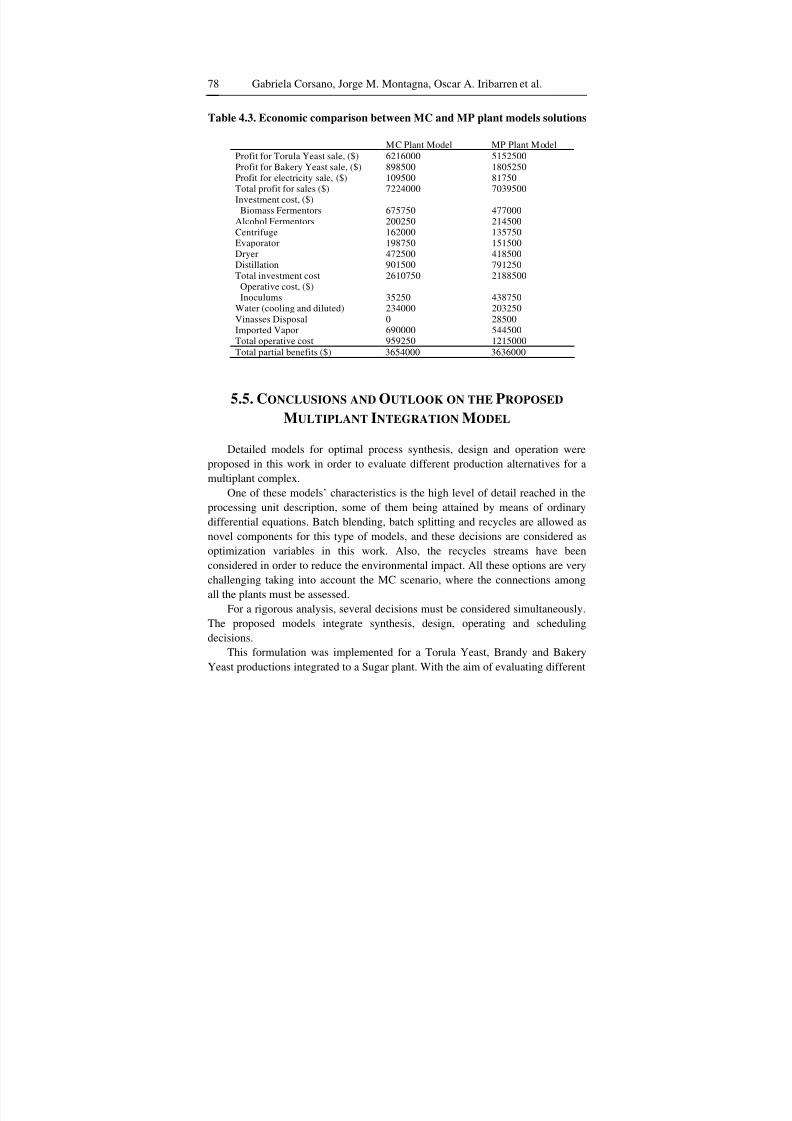
8/7/2019 Corsano G. Montagna J.M. Iribarren O.A. Aguirre P.A. Mathematical Modeling Approaches for Optimization of Chemic…
http://slidepdf.com/reader/full/corsano-g-montagna-jm-iribarren-oa-aguirre-pa-mathematical-modeling 90/103
Gabriela Corsano, Jorge M. Montagna, Oscar A. Iribarren et al.78
Table 4.3. Economic comparison between MC and MP plant models solutions
MC Plant Model MP Plant ModelProfit for Torula Yeast sale, ($)Profit for Bakery Yeast sale, ($)Profit for electricity sale, ($)Total profit for sales ($)
62160008985001095007224000
51525001805250817507039500
Investment cost, ($)Biomass Fermentors
Alcohol FermentorsCentrifugeEvaporatorDryerDistillationTotal investment cost
6757502002501620001987504725009015002610750
4770002145001357501515004185007912502188500
Operative cost, ($)Inoculums
Water (cooling and diluted)Vinasses DisposalImported VaporTotal operative cost
352502340000690000959250
438750203250285005445001215000
Total partial benefits ($) 3654000 3636000
5.5. CONCLUSIONS AND OUTLOOK ON THE PROPOSED
MULTIPLANT INTEGRATION MODEL
Detailed models for optimal process synthesis, design and operation were
proposed in this work in order to evaluate different production alternatives for a
multiplant complex.
One of these models’ characteristics is the high level of detail reached in the
processing unit description, some of them being attained by means of ordinary
differential equations. Batch blending, batch splitting and recycles are allowed as
novel components for this type of models, and these decisions are considered as
optimization variables in this work. Also, the recycles streams have been
considered in order to reduce the environmental impact. All these options are very
challenging taking into account the MC scenario, where the connections among
all the plants must be assessed.
For a rigorous analysis, several decisions must be considered simultaneously.
The proposed models integrate synthesis, design, operating and scheduling
decisions.
This formulation was implemented for a Torula Yeast, Brandy and Bakery
Yeast productions integrated to a Sugar plant. With the aim of evaluating different

8/7/2019 Corsano G. Montagna J.M. Iribarren O.A. Aguirre P.A. Mathematical Modeling Approaches for Optimization of Chemic…
http://slidepdf.com/reader/full/corsano-g-montagna-jm-iribarren-oa-aguirre-pa-mathematical-modeling 91/103
Process Integration 79
production scenarios, the solution of MC model was compared with that obtained
in the previous section for a MP model. For the study case, several results were
analyzed; some tradeoffs between process and design variables were presentedtogether with the economic impact in each case. Finally the conclusions for each
comparison were reported.
Further on these specific results, this work emphasizes the significant value of
formulations that take into account all involved decisions simultaneously so as to
reach effective solutions.
The idea presented in this work can be applied to other process productions,
and the analysis can be performed according to different variations on the
operative conditions.

8/7/2019 Corsano G. Montagna J.M. Iribarren O.A. Aguirre P.A. Mathematical Modeling Approaches for Optimization of Chemic…
http://slidepdf.com/reader/full/corsano-g-montagna-jm-iribarren-oa-aguirre-pa-mathematical-modeling 92/103
8/7/2019 Corsano G. Montagna J.M. Iribarren O.A. Aguirre P.A. Mathematical Modeling Approaches for Optimization of Chemic…
http://slidepdf.com/reader/full/corsano-g-montagna-jm-iribarren-oa-aguirre-pa-mathematical-modeling 93/103
Chapter 6
GENERAL SUMMARY AND SUGGESTIONS FOR
FURTHER READING
This chapter has been prepared in order to present different applications of
mathematical modeling in chemical engineering. Really it is a powerful tool to
solve significant problems in the different stages of the chemical process lifecycle.
We have chosen a particular context, and modelled different problems related to
batch processes. The obtained conclusions have allowed us to present the valuable
results that can be attained when complete and comprehensive models have been
developed.
The detailed models provided in this chapter have been focused on the
simultaneous optimization of the synthesis, design, operation, and scheduling of chemical processes. These models include decisions of plant configuration,
material and energy balances, design equations, product and by-products
specifications constraints, environmental considerations, integration processes
decisions, blending and recycles constraints, economics objective functions,
among others. Thus, we have posed models that show one of the main advantages
of mathematical modeling: decisions can be made taking into account all the
elements involved and the trade-offs among them. Usually, different actors, areas,
stages, etc. may have different and opposite goals that must be related and
coordinated in order to achieve the optimal results for the global system.
In the first section, a concise overview of basic concepts and definitions wasprovided, in order that the reader can be introduced in process engineering models
and some methodologies used in this area. For further reading, a classic text of
this area is due to Biegler, Grossmann, and Westerberg (1997).
In the second section, a novel superstructure model is presented in order to
obtain the optimal plant configuration simultaneously with the optimal plant
8/7/2019 Corsano G. Montagna J.M. Iribarren O.A. Aguirre P.A. Mathematical Modeling Approaches for Optimization of Chemic…
http://slidepdf.com/reader/full/corsano-g-montagna-jm-iribarren-oa-aguirre-pa-mathematical-modeling 94/103
Gabriela Corsano, Jorge M. Montagna, Oscar A. Iribarren et al.82
design and operation. The main characteristic of this approach remains in the fact
that discrete decisions are taken without resort to integer optimization variables.
The details of this approach and more examples can be found in Corsano et al.(2004, 2006a).
In the third section a heuristic procedure for finding the optimal mixed
product campaign for a multipurpose/multiproduct plant is presented. The
approach consists in two steps: first a relaxed model is solved in order to obtain
the plant configuration and the relationship between the numbers of batch of each
product. Then, according to that relationship, a mixed product campaign model is
proposed and solved. Sometimes, in this model, the designer criteria or
knowledge can influence in the campaign sequence selection and it can be taken
into account. For further details of this methodology see Corsano et al. (2007).
For others approaches for mixed product campaign models see Birewar andGrossmann (1989, 1990), Xia and Macchietto (1997), Lin and Floudas (2001),
and Ierapetritou et al. (1999).
In the fourth section a model for the processes integration in a multiplant
complex is developed. The model stresses the optimization of all the production
processes embedded in an overall model, emphasizing the relations among all
them. The use of recycles streams in order to reduce the environmental impact is
considered. The presented model for optimal synthesis, design, operation and
scheduling of MC provide a tool for the alternatives analysis of different
configurations. In addition, the economical tradeoffs between each production
scheme were established and assessed as well as a comparison with amultiproduct plant configuration.
In all the sections, numerical examples corresponding to the Sugar Cane
industry and its derivative productions were posed. Although the Sugar Cane
example serves as good case of processes integration, the proposed models can be
modified to other industrial and engineering examples where several decisions
and different alternatives can be analyzed.
8/7/2019 Corsano G. Montagna J.M. Iribarren O.A. Aguirre P.A. Mathematical Modeling Approaches for Optimization of Chemic…
http://slidepdf.com/reader/full/corsano-g-montagna-jm-iribarren-oa-aguirre-pa-mathematical-modeling 95/103
REFERENCES
Atkinson, K. E. An Introduction to Numerical Analysis. Second Edition. John
Wiley & Sons; New York, 1989.
Barrera M. D.; Evans L. B. Optimal Design and Operation of Batch Processes.
Chem. Engng. Comm. 1989, 82, 45.
Bhatia, T. K.; Biegler, L.T. Dynamic Optimisation in the Design and Scheduling
of Multiproduct Batch Plants Ind. Eng. Chem. Res. 1996, 35, 2234.
Biegler, L. T.; Grossmann, I. E.; Westerberg, A. W. Systematic Methods of
Chemical Process Design. Prentice Hall International Series in the Physical
and Chemical Engineering Sciences; New Jersey, 1997.
Birewar, D. B.; Grossmann, I. E. Incorporating scheduling in the optimal design
of multiproduct batch plant. Comp. & Chem. Eng. 1989, 13, 141.
Birewar, D. B.; Grossmann, I. E. Simultaneous synthesis, sizing, and schedulingof multiproduct batch plants. Ind. Eng. Chem. Res. 1990, 29, 2242.
Brooke A.; Kendrick D.; Meeraus A.; Raman R. GAMS, A User Guide. Scientific
press, Calif,1998.
Corsano, G.; Iribarren, O. A.; Montagna, J. M.; Aguirre, P.A.. Batch Fermentation
Networks Model for Optimal Synthesis, Design and Operation. Ind. Eng.
Chem. Res. 2004, 43, 4211.
Corsano, G., Montagna, J.M, Aguirre, P.A., Iribarren, O.A. Design and Operation
Issues using NLP Superstructure modeling. Applied Mathematical Modeling
2006a, 30 (9), 974.
Corsano, G.; Iribarren, O. A.; Montagna, J. M.; Aguirre, P.A.; González Suárez,E. Economic Tradeoffs involved in the Design of Fermentation Processes
with Environmental Constraints. Chemical Engineering Research and Design
2006b, 84 (10), 1.
8/7/2019 Corsano G. Montagna J.M. Iribarren O.A. Aguirre P.A. Mathematical Modeling Approaches for Optimization of Chemic…
http://slidepdf.com/reader/full/corsano-g-montagna-jm-iribarren-oa-aguirre-pa-mathematical-modeling 96/103
Gabriela Corsano, Jorge M. Montagna, Oscar A. Iribarren et al.84
Corsano, G.; Montagna, J. M.; Iribarren, O. A.; Aguirre, P.A. Processes
Integration: Multiplant Complex vs Multipurpose Plant Assessment. Ind. Eng.
Chem. Res. 2006c, 45, 4253.Corsano, G., Montagna, J.M, Aguirre, P.A., Iribarren, O.A. A Heuristic Method
for the Optimal Synthesis and Design of Batch Plants Considering Mixed
Product Campaigns. Ind. & Eng. Chem. Res. 2007, 46 (9), 2769.
Duran, M. A.; Grossmann, I. E. Outer-Approximation Algorithm for a Class of
Mixed-Integer Nonlinear Programs. Mathematical Programming 1986, 36
(3), 307.
Grossmann, I. E.; Sargent, R. W. H. Optimum design of multipurpose chemical
plants. Industrial and Engineering Chemistry Process Design and
Development 1979, 18 (2), 343.
Ierapetritou, M. G.; Floudas, C. A.; Vasantharajan S.; Cullick A. S. OptimalLocation of Vertical Wells: Decomposition Approach . AIChE Journal 1999,
45(4), 844.
Jackson, J.R.; Grossmann I.E. Temporal decomposition scheme for nonlinear
multisite production planning and distribution models. Ind. Eng. Chem. Res.
2003, 42, 3045.
Kallrath, J. Combined strategic and operational planning: An MILP success story
in chemical industry. OR Spectrum 2002, 24, 315 – 341.
Knopf F. C.; Okos M. R.; Reklaitis G. V. Optimal Design of Batch / Semi
continuous Processes. Ind. Eng. Chem. Process Des. Dev. 1982, 21, 79.
Lee, H-K.; Lee I-B.; Reklaitis, G.V. Capacity expansion problem of multisitebatch plants with production and distribution. Comp. & Chem. Engn. 2000,
24, 1597.
Lin, X.; Floudas, C. A. Design, synthesis and scheduling of multipurpose batch
plants via an effective continuous-time formulation. Comp. & Chem. Engn.
2001, 25, 665.
Montagna J. M.; Vecchietti A. R.; Iribarren O. A.; Pinto J. M.; Asenjo J. A.
Optimal Design of Protein Production Plants with Time and Size Factor
Process Models. Biotechnol. Prog. 2000, 16 , 228.
Ravemark D. E.; Rippin D. W. T. Optimal Design of Multiproduct Batch Plants.
Comput. Chem. Engng. 1998, 22, 177.
Salomone H. E.; Iribarren O. A. Posynomial Modeling of Batch Plants. Comput.
Chem. Engng. 1992, 16 , 173.
Salomone H. E.; Montagna J. M.; Iribarren O. A. Dynamic Simulations in the
Design of Batch Processes. Comput. Chem. Engng. 1994, 18, 191.
8/7/2019 Corsano G. Montagna J.M. Iribarren O.A. Aguirre P.A. Mathematical Modeling Approaches for Optimization of Chemic…
http://slidepdf.com/reader/full/corsano-g-montagna-jm-iribarren-oa-aguirre-pa-mathematical-modeling 97/103
References 85
Varvarezos, D. K.; Grossmann, I. E.; Biegler, L. T. An Outer-Approximation
Method for Multiperiod Design Optimization. Ind. Eng. Chem. Res. 1992, 31,
1466.Viswanathan, J.; Grossmann, I. E. Combined penalty function and outer-
approximation method for MINLP optimization. Comp. & Chem. Engn. 1990,
14 (7), 769.
Voudouris, V. T.; Grossmann, I. E. MILP model for scheduling and design of a
special class of multipurpose batch plants. Comp. & Chem. Engng. 1996, 20
(11), 1335.
Wu, M. D. ; Ierapetritou, M. Hierarchical approach for production planning and
scheduling under uncertainty, Chem. Eng. Process 2007, in press.
Xia, Q.; Macchietto, S. Design and synthesis of batch plantsMINLP solution
based on a stochastic method. Comp. & Chem. Engn. 1997, 21, S697.Yeh N. C.; Reklaitis G. V. Synthesis of Batch / Semicontinuous Processes.
Comput. Chem. Engng. 1987, 11, 639.
Zhang, X.; Sargent, R. W. H. The optimal operation of mixed production
facilities- a general formulation and some solution approaches for the
solution. In Proceeding of 5th
Int. Symp. Process Systems Engineering 1994,
171. Korea.
Zhang, X.; Sargent, R. W. H. The optimal operation of mixed production facilities
- extensions and improvements. Comp. & Chem. Engn. 1996, S20, 1287.

8/7/2019 Corsano G. Montagna J.M. Iribarren O.A. Aguirre P.A. Mathematical Modeling Approaches for Optimization of Chemic…
http://slidepdf.com/reader/full/corsano-g-montagna-jm-iribarren-oa-aguirre-pa-mathematical-modeling 98/103
8/7/2019 Corsano G. Montagna J.M. Iribarren O.A. Aguirre P.A. Mathematical Modeling Approaches for Optimization of Chemic…
http://slidepdf.com/reader/full/corsano-g-montagna-jm-iribarren-oa-aguirre-pa-mathematical-modeling 99/103
INDEX
A
agricultural, 3
alcohol, 51, 54, 57, 63, 64, 65, 75, 77
algorithm, 15
alternative, 9, 14, 16, 17, 18, 20, 22, 23, 24,
25, 29, 36, 74
alternatives, 9, 13, 14, 16, 17, 18, 20, 23, 24,
25, 29, 30, 32, 34, 36, 54, 68, 71, 74, 78, 82
application, 15
attention, 10, 67
availability, 10, 13
B
bacteria, 21
benefits, 76
biomass, 20, 21, 22, 24, 25, 29, 30, 31, 39, 40,
51, 54, 57, 65, 69, 75, 77
biotechnological, 15
bottleneck, 5
bottlenecks, 5, 7
bounds, 14, 31, 32, 74
by-products, 37, 68, 81
C
campaigns, 8, 36, 38, 45, 63
capacity, 4, 5, 7, 14, 17, 84
capital, 10
capital cost, 10
C-C, 45chemical, ix, 1, 3, 4, 14, 36, 67, 81, 84
chemical engineering, ix, 1, 36, 81
chemical industry, 84
chemicals, 3
classification, 3, 4, 5
codes, 15
community, 7
complexity, 8, 35, 53
components, 20, 39, 66, 78
composition, 7, 21
computer, 15
concentration, 14, 21, 22, 39, 40, 68, 69, 75,
77
configuration, 1, 11, 16, 17, 25, 29, 31, 32, 36,
38, 42, 44, 47, 51, 54, 57, 63, 65, 68, 72,
75, 81, 82
Congress, v
constraints, 1, 4, 7, 9, 10, 14, 18, 20, 22, 29,
31, 32, 36, 38, 39, 40, 41, 43, 45, 46, 47,
48, 50, 51, 54, 57, 60, 61, 63, 64, 65, 69,
70, 71, 72, 81
consumption, 53
convergence, 34
convex, 14, 30, 32
costs, 17, 18, 22, 25, 36, 43, 60, 65, 66, 71,
74, 76
Cp, 16, 17
CPU, 24, 31, 34, 74
8/7/2019 Corsano G. Montagna J.M. Iribarren O.A. Aguirre P.A. Mathematical Modeling Approaches for Optimization of Chemic…
http://slidepdf.com/reader/full/corsano-g-montagna-jm-iribarren-oa-aguirre-pa-mathematical-modeling 100/103
Index88
D
death, 21, 40death rate, 21, 40
decision making, 7, 8
decisions, ix, 1, 8, 9, 13, 15, 53, 66, 68, 72,
73, 74, 78, 79, 81, 82
decomposition, 10, 72, 84
definition, 47, 57, 61
degradation, 54
degrees of freedom, 7
demand, 15, 18, 71, 77
dependent variable, 7
derivatives, 51, 53, 72
differential equations, 8, 10, 14, 21, 39, 41,68, 70, 78
discrete variable, 31
discretization, 25, 39
distillation, 3, 51, 60, 63, 64, 65, 77
distribution, 50, 84
drying, 51
duplication, 5, 6, 7, 13, 14, 16, 17, 24, 29, 72
E
earnings, 36, 43, 65economic, 15, 37, 62, 77, 79
economics, 81
effluent, 44
effluents, 70
electricity, 51, 53, 63, 65, 72, 76
electronic, v
electrostatic, v
energy, 4, 37, 42, 67, 68, 69, 70, 72, 81
engineering, ix, 1, 2, 24, 36, 81, 82
environmental, 11, 68, 78, 81, 82
environmental impact, 78, 82
environmental issues, 11equipment, 3, 5, 7, 13, 15, 18, 20, 22, 25, 29,
35, 60, 62, 74
ethanol, 20, 21, 22, 23, 24, 25, 28, 29, 30, 31,
32
evaporation, 51
expert, v
extraction, 53
F
feeding, 7, 14
fermentation, 7, 13, 20, 21, 23, 24, 28, 29, 30,
31, 32, 51, 54, 57, 64, 65, 72, 75, 77
flexibility, 35
flow, 68
freedom, 7
G
generation, 32goals, 81
growth, 21, 40
growth rate, 40
H
handling, 20, 30, 32
heuristic, 11, 14, 38, 53, 66, 72, 82
horizon, 8, 15, 17, 37, 40, 54, 60, 70, 75
human, 77
I
incomes, 76
industrial, 11, 15, 42, 82
industry, ix, 1, 3, 4, 7, 82, 84
injury, v
integration, 4, 6, 8, 10, 11, 39, 51, 68, 72, 77,
81, 82
intrinsic, 8
investment, 22, 36, 43, 60, 62, 65, 66, 68, 71,
76, 77
J
judge, 34
8/7/2019 Corsano G. Montagna J.M. Iribarren O.A. Aguirre P.A. Mathematical Modeling Approaches for Optimization of Chemic…
http://slidepdf.com/reader/full/corsano-g-montagna-jm-iribarren-oa-aguirre-pa-mathematical-modeling 101/103
Index 89
K
KH, 26Korea, 85
L
language, 7
lead, 8, 35
lifecycle, ix, 81
limitation, 42
linear, 8, 9, 15
linear function, 9
linear programming, 8literature, 8, 9, 10, 36, 77
logistics, 7
long period, 54
M
magnetic, v
market, 69
mathematical, ix, 1, 2, 7, 8, 9, 11, 45, 53, 74,
81
mechanical, vmixing, 3, 37, 67
modeling, ix, 1, 9, 15, 34, 39, 67, 81, 83
models, ix, 1, 2, 7, 8, 9, 10, 13, 14, 15, 20, 24,
29, 30, 31, 32, 40, 41, 45, 53, 54, 60, 62,
65, 66, 70, 74, 78, 81, 82, 84
modules, 10
molasses, 51, 53, 72, 76
N
NA, 45
Nb, 45, 57, 61, 64
NC, 45
network, 15
New Jersey, 83
New York, iii, v, 83
NIS, 4
nonlinear, 8, 9, 10, 84
O
optimization, ix, 1, 7, 8, 9, 10, 11, 14, 15, 16,36, 38, 39, 45, 46, 48, 51, 54, 66, 67, 68,
74, 78, 81, 82, 85
OR, 84
ordinary differential equations, 78
P
paper, 41
parameter, 45
penalty, 85
performance, 7, 8, 10, 14, 77periodic, 3
permit, 9
pharmaceutical, 3
planning, 1, 2, 4, 7, 8, 10, 11, 67, 84, 85
planning decisions, 8
plants, 4, 7, 10, 11, 14, 15, 32, 35, 67, 68, 69,
70, 71, 72, 77, 78, 83, 84, 85
power, ix, 36, 43, 51
power stations, 51
preparation, v
prices, 68
processing variables, 1, 7, 68production, 1, 3, 4, 7, 8, 10, 14, 16, 18, 20, 21,
22, 23, 24, 25, 35, 36, 37, 38, 39, 40, 41,
42, 43, 44, 45, 46, 47, 48, 49, 50, 51, 53,
54, 55, 57, 60, 62, 65, 66, 67, 68, 69, 70,
71, 74, 76, 77, 78, 79, 82, 84, 85
production targets, 1, 68
profit, 36, 43, 63, 68
profits, 71, 74
program, 10, 29
programming, 8, 9
property, v
R
Raman, 83
range, 3, 10
raw material, 1, 4, 13, 14, 35, 43, 67, 70
8/7/2019 Corsano G. Montagna J.M. Iribarren O.A. Aguirre P.A. Mathematical Modeling Approaches for Optimization of Chemic…
http://slidepdf.com/reader/full/corsano-g-montagna-jm-iribarren-oa-aguirre-pa-mathematical-modeling 102/103
Index90
raw materials, 1, 4, 14, 35, 67, 70
reaction rate, 13, 24
reading, 81
recycling, 67, 72
reduction, 65, 77
relationship, 13, 20, 46, 82
relationships, 68, 74
relaxation, 38, 39
repetitions, 46
resolution, 9, 14, 15, 31, 32, 65, 74
resources, 8, 35, 36, 37, 42, 43, 67, 68, 69, 72,
74, 76, 77
rice, 68
robustness, 15
S
sales, 43, 65, 68, 71, 76
satisfaction, 60
saturation, 21
savings, 36
scheduling, ix, 1, 2, 4, 7, 8, 10, 11, 35, 36, 38,
39, 44, 50, 51, 53, 65, 66, 67, 68, 74, 78,
81, 82, 83, 84, 85
sequencing, 4
series, 5, 7, 13, 14, 15, 16, 17, 24, 25, 29, 30,
32, 36, 41, 42, 46, 48, 54, 72, 75
services, v
sharing, 35
short-term, 8
simulation, 10
solutions, 2, 10, 11, 15, 27, 31, 33, 36, 50, 65,
77, 78, 79
stages, 5, 7, 8, 10, 13, 14, 15, 16, 17, 18, 20,
21, 22, 23, 24, 29, 30, 31, 36, 39, 40, 41,
42, 49, 51, 60, 61, 77, 81
stochastic, 85
storage, 4, 7strategic, 7, 84
strategic planning, 7
strategies, 35
streams, 3, 20, 36, 68, 78, 82
substrates, 21, 22, 51
sugar, 1, 21, 22, 51, 53
superposition, 47, 48, 63, 65
synthesis, ix, 1, 2, 7, 8, 10, 11, 13, 14, 35, 38,
51, 53, 54, 57, 65, 66, 67, 68, 74, 77, 78,
81, 82, 83, 84, 85
systematic, 14
T
tanks, 4
targets, 1, 68
Ti, 47
ticks, 7
time, 3, 5, 7, 8, 10, 15, 16, 17, 18, 20, 22, 24,
25, 29, 31, 34, 37, 39, 40, 41, 42, 46, 47,
48, 50, 54, 57, 60, 61, 62, 64, 65, 69, 70,
74, 75, 77, 84
timing, 4
total product, 43, 60
trade, ix, 1, 10, 68, 75, 77, 81
trade-off, ix, 1, 10, 68, 75, 77, 81
traditional model, 29
transfer, 4, 16, 46, 75
transference, 77
TT, 57, 61
U
uncertainty, 85
unit cost, 17
V
values, 20, 25, 39, 54, 62, 74
vapor, 51, 53, 72, 76
variable, 16, 22, 25, 29, 39, 45, 53, 68
variables, 1, 7, 8, 9, 10, 13, 14, 15, 21, 25, 29,
30, 31, 37, 39, 41, 50, 52, 53, 54, 57, 60,
61, 62, 64, 65, 66, 68, 70, 71, 74, 75, 78,79, 82
velocity, 21
versatility, ix, 74

8/7/2019 Corsano G. Montagna J.M. Iribarren O.A. Aguirre P.A. Mathematical Modeling Approaches for Optimization of Chemic…
http://slidepdf.com/reader/full/corsano-g-montagna-jm-iribarren-oa-aguirre-pa-mathematical-modeling 103/103
Index 91
W
waste, 51water, 22, 51
workers, 77
Y
yeast, 32yield, 21, 77
Recommended