Copyright
by
Shan Huang
2015

The Dissertation Committee for Shan Huang Certifies that this is the approved
version of the following dissertation:
Fast Forward Modeling and Inversion of Borehole Sonic Measurements
using Spatial Sensitivity Functions
Committee:
Carlos Torres-Verdín, Supervisor
Kamy Sepehrnoori
Jon E. Olson
Mukul M. Sharma
Kyle T. Spikes

Fast Forward Modeling and Inversion of Borehole Sonic Measurements
using Spatial Sensitivity Functions
by
Shan Huang, B.E., M.E.
Dissertation
Presented to the Faculty of the Graduate School of
The University of Texas at Austin
in Partial Fulfillment
of the Requirements
for the Degree of
Doctor of Philosophy
The University of Texas at Austin
May 2015

Dedication
Dedicated to my family, for their unconditional support and excruciating tolerance.

v
Acknowledgements
I would like to express my sincere gratitude to my supervising professor, Dr.
Carlos Torres-Verdín for his consistent support and valued guidance that shape my
thought processes during my graduate study.
I am grateful to the many researchers and students in our department, both past
and present, that aided me in my research: Ruijia Wang, Pawel J. Matuszyk, Qinshan
Yang, Jun Ma, Wilberth C. Herrera, Shuang Gao, Wei Li, Wei Yu, Kan Wu, Pengpeng
Qi, Hyung Joo Lee, Oyinkansola Ajayi, Olabode Ijasan, Haryanto Adiguna, Siddharth
Mishra, Tatyana Torskaya, Hamid Beik, Vahid Shabro, Amir Frooqnia, Shaina Kelly,
Essi Kwabi, Paul Sayer, Elsa Maalouf, and Chicheng Xu. I am also grateful to Dr. Roger
Terzian and Tim Quinn for their helpful computer support. Special thanks to Rey
Casanova for his administrative support at the formation evaluation research consortium. I
also wish to thank Frankie Hart for her help and support in the petroleum engineering
department.
I give much appreciation to my dissertation committee members: Drs. Kamy
Sepehrnoori, Jon E. Olson, Mukul M. Sharma, and Kyle T. Spikes for their time, support,
and reviews of this dissertation.
I acknowledge the Texas Advanced Computing Center (TACC) at The University
of Texas at Austin for providing high-performance computing resources that contributed
to the research results reported in this dissertation.
I was fortunate to spend two summers as an intern at Exxonmobil Upstream
Research Company, which expanded my knowledge and skills in ways that improved my

vi
ability to carry out my research. For that, I thank especially Pingjun Guo, Xianyun Wu,
Jinjuan Zhou, Quinn Passey, Alex Martinez, and Christopher Harris.
I am immensely grateful to my family and friends for their support and patience
throughout this journey. To Chunguang Huang, Zhihuai Li, Yang Liu, and Tuantuan,
thank you so much for all your perseverance, prayers, and yearn for my success.
Finally, this research was made possible through the funding of the University of
Texas at Austin’s Research Consortium on Formation Evaluation, jointly sponsored by
Afren, Anadarko, Apache, Aramco, Baker-Hughes, BG, BHP Billiton, BP, Chevron,
China Oilfield Services LTD., ConocoPhillips, Det Norske, ENI, ExxonMobil,
Halliburton, Hess, Maersk, Mexican Institute for Petroleum, ONGC, OXY, Petrobras,
PTT Exploration and Production, Repsol, RWE, Schlumberger, Shell, Southwestern
Energy, Statoil, TOTAL, Weatherford, Wintershall, and Woodside Petroleum Limited.

vii
Fast Forward Modeling and Inversion of Borehole Sonic Measurements using
Spatial Sensitivity Functions
Shan Huang, Ph.D.
The University of Texas at Austin, 2015
Supervisor: Carlos Torres-Verdín
Borehole sonic measurements are widely used by petrophysicists to estimate in-
situ dynamic elastic properties of rock formations. The estimated formation properties
typically guide the interpretation of seismic amplitude measurements in the exploration
and development of hydrocarbon reservoirs. Due to limitations in vertical resolution,
borehole sonic measurements (sonic logs) provide spatially averaged values of formation
properties in thinly bedded rocks. In addition, mud-filtrate invasion and near-wellbore
formation damage can bias the elastic properties estimated from sonic logs. The
interpretation of sonic logs in high angle (HA) and horizontal (HZ) wells is even more
challenging because of three-dimensional geometrical effects and anisotropy.
A reliable approach to account for geometrical effects in the interpretation of
sonic logs is the implementation of forward modeling and inversion techniques.
However, the computation time required to model the direct problem, namely wave
propagation in the borehole environment, severely constraints the usage of inversion
approaches in sonic-log interpretation. This dissertation develops new methods for the
rapid simulation of sonic logs using the concept of spatial sensitivity functions. Sonic
spatial sensitivity functions are equivalent to the Green’s function of a particular sonic
measurement; they also serve as weighting matrices to map formation elastic properties
viii
into the respective measurement space. Application of sensitivity functions to challenging
synthetic examples verifies that the maximum relative error in the modeled sonic logs is
lower than 3% for flexural, Stoneley, and compressional (P-) and shear (S-) modes.
Compared to rigorous numerical simulations, the new fast sonic modeling method
reduces computation time by 98%.
Using the fast sonic simulation algorithm, we develop an inversion method that
combines multi-frequency flexural dispersion and P- and S- mode slowness logs to
estimate layer-by-layer compressional and shear slownesses of rock formations. Synthetic
verification examples as well as interpretation of field cases indicate that the estimated
formation compressional and shear slownesses are within 3% of true model properties,
exhibiting a maximum uncertainty of 6%. When compared to conventional sonic-log
interpretation, the new inversion-based method effectively reduces shoulder-bed effects
and relative errors in estimated properties by 15%, while the vertical resolution of sonic
logs is improved from 1.83 m to 0.5 m.
Finally, we show that multi-mode wave interference in HA/HZ wells makes it
difficult to identify the low-frequency slowness asymptote of the flexural mode. We
extend the sensitivity method to three dimensions to approach this latter problem and to
model high-frequency dispersion logs. Because the calculated P-mode slowness log
exhibits strong dependence to processing parameters, conventional waveform semblance-
based processing becomes inadequate in HA wells. We introduce a new P-arrival slowness
log to circumvent wave mode interference and to avoid semblance calculations.
Additionally, we also develop a one-dimensional integration method to rapidly model P-
arrival slowness logs when HA/HZ wells penetrate anisotropic thin beds. The fast
modeling algorithm generates synthetic logs that match sonic logs simulated with rigorous
modeling procedures within 5% while providing a 99% reduction in computation time.
ix
Table of Contents
List of Tables ......................................................................................................... xi
List of Figures ...................................................................................................... xiii
Chapter 1: Introduction ............................................................................................1
1.1 Problem Statement .................................................................................1
1.2 Research Objectives ...............................................................................7
1.3 Method Overview ..................................................................................9
1.4 Outline of the Dissertation ...................................................................12
Chapter 2: Spatial sensitivity functions for rapid simulation of borehole sonic
measurements in vertical wells .....................................................................14
2.1 Introduction ..........................................................................................15
2.2 Definition of the Sonic Sensitivity Functions ......................................18
2.3 Axial Sensitivity Functions ..................................................................21
2.4 Axial-Radial Sensitivity Functions ......................................................31
2.5 Semi-Analytical Axial Sensitivity Functions.......................................39
2.6 Semi-Analytical Axial-Radial Sensitivity Functions ...........................47
2.7 Axial Sensitivity Functions of Non-Dispersive Modes .......................52
2.8 Modeling Dispersion in Thin Beds ......................................................55
2.9 Modeling dispersion in Thin Beds with Invasion ................................67
2.10 Modeling Non-Dispersive Mode Slowness Logs ................................71
2.11 Discussion ............................................................................................79
2.12 Conclusions ..........................................................................................79
Chapter 3: Inversion-based interpretation of borehole sonic measurements using
semi-analytical spatial sensitivity functions .................................................81
3.1 Introduction ..........................................................................................82
3.2 Esitmation of Formation Elastic Properties from Flexural Dispersion Data
..............................................................................................................86
3.3 Joint Inversion of Compressional and Shear Slownesses ....................97
3.4 Conclusions ........................................................................................122

x
Chapter 4: Fast forward modeling of borehole sonic measurements in high-angle and
horizontal wells ...........................................................................................124
4.1 Introduction ........................................................................................125
4.2 Modeling Guided-Mode Dispersions in HA/HZ Wells .....................129
4.3 STC Processing in HA/HZ Wells ......................................................140
4.4 P-arrival Slowness in HA/HZ Wells ..................................................149
4.5 Estimation of P-arrival Slowness using Ray-Tracing Method ..........153
4.6 One-Dimensional Layered Model in HA/HZ Wells ..........................159
4.7 Fast Forward Modeling: Method .......................................................165
4.8 Fast Forward Modeling: Results ........................................................169
4.9 Conclusions ........................................................................................174
Chapter 5: Summary, Conclusions, and Future Research Recommendations .....176
5.1 Summary ............................................................................................176
5.2 Conclusions ........................................................................................180
5.2.1 General conclusions about the best practices for petrophysical
modeling and inversion of borehole sonic measurements ........180
5.2.2 Spatial sensitivity functions for fast-forward modeling of borehole
sonic measurements ..................................................................183
5.2.3 Inversion-based interpretation of borehole sonic logs ..............185
5.2.4 Fast-forward modeling of dispersion and P-arrival slowness
measurements in HA/HZ wells .................................................186
5.3 Recommended Best Practices ............................................................187
5.4 Future Research Recommendations ...................................................189
List of Symbols ....................................................................................................192
List of Acronyms .................................................................................................196
References ............................................................................................................198
Vita .....................................................................................................................204

xi
List of Tables
Table 2.1: Elastic properties assumed for borehole fluid and rock formations. 30
Table 2.2: Elastic and geometrical properties assumed for the logging tool. ....30
Table 2.3: Assumed layer properties. .................................................................58
Table 2.4: Properties assumed for the rock formation with invaded thin beds. .70
Table 2.5: Properties assumed for the synthetic rock formations for shear and
compressional slowness modeling. ...................................................78
Table 3.1: Assumed layer properties for the synthetic formation model with 15 thin
beds shown in Figure 1. Layer1 is the shallowest, while layer 15 is the
deepest...............................................................................................89
Table 3.2: Inversion results of shear slowness for the synthetic formation with 15
thin beds (Figure 3.1). Layer1 is the shallowest, while layer 15 is the
deepest...............................................................................................92
Table 3.3: Assumed layer properties for the synthetic formation models. Layer1 is
the shallowest, while layer 5 is the deepest in both models..............98
Table 3.4: Estimation of compressional and shear slownesses for the synthetic
models in Table 3. Layer1 is the shallowest, while layer 5 is the deepest
in each model. .................................................................................104
Table 3.5: Joint inversion results for the synthetic formation with 15 thin beds
(Figure 3.1). Layer1 is the shallowest, while layer 15 is the deepest.107
Table 3.6: Joint inversion results for the field case (Figure 3.3). Layer1 is the
shallowest, while layer 15 is the deepest. .......................................113
Table 3.8: Joint inversion results for the field data shown in Figure 3.14. Layer1 is
the shallowest, while layer 19 is the deepest. .................................120

xii
Table 4.1: Elastic properties of the formation layers. BG represents background
formation, L1 to L3 denote the layers. L1 and L3 are the deepest and the
shallowest, respectively. .................................................................130
Table 4.2: Elastic and geometrical properties of the wireline logging tool. ....130
Table 4.3: Geometrical parameters of the well shown in Figure 4.3. ..............136
Table 4.4: Equivalent isotropic parameters for the model shown in Figure 4.3.137
Table 4.5: Parameters of the formations shown in Figure 4.1. ........................142
Table 4.6: Properties of the layers shown in Figure 4.21.................................170
Table 4.7: Properties of the formations shown in Figure 4.23. ........................172

xiii
List of Figures
Figure 2.1: Axial sensitivity of the flexural mode to (a) shear velocity, (b)
compressional velocity, and (c) density perturbations in a fast formation.
Receiver locations are identified with thick black lines on the tool
mandrel. ............................................................................................26
Figure 2.2: Axial sensitivity of the Stoneley mode to (a) shear velocity, (b)
compressional velocity, and (c) density perturbations in a fast formation.
Receiver locations are identified with thick black lines on the tool
mandrel. ............................................................................................27
Figure 2.3: Axial sensitivity of the flexural mode to (a) shear velocity, (b)
compressional velocity, and (c) density perturbations in a slow
formation. Receiver locations are identified with thick black lines on the
tool mandrel. .....................................................................................28
Figure 2.4: Axial sensitivity of the Stoneley mode to (a) shear velocity, (b)
compressional velocity, and (c) density perturbations in a slow
formation. Receiver locations are identified with thick black lines on the
tool mandrel. .....................................................................................29
Figure 2.5: Axial-radial sensitivity of the flexural mode to shear velocity
perturbations at (a) 2 kHz, (b) 3 kHz, (c) 4 kHz, (d) 5 kHz, (e) 6 kHz,
and (f) 7 kHz, calculated in a slow formation. Receiver locations are
identified with thick black lines on the tool mandrel. Each panel is
displayed with a different color scale (shown to the right of the color
map). .................................................................................................34

xiv
Figure 2.6: (a) Axial sensitivity curves and (b) radial sensitivity curves obtained
from axial-radial sensitivity functions. Receiver locations are identified
with thick black lines on the tool mandrel. .......................................35
Figure 2.7: Axial-radial sensitivity of the flexural mode to shear velocity
perturbations at 2 kHz, calculated from the transmitter to the top
receiver. Receiver locations are identified with thick black lines on the
tool mandrel. .....................................................................................36
Figure 2.8: Flexural mode axial-radial sensitivities to compressional slowness
perturbations at (a) 3 kHz, (b) 5 kHz, and (c) 7 kHz. Flexural mode
axial-radial sensitivities to density perturbation at (d) 3 kHz, (e) 5 kHz,
and (f) 7 kHz. Receiver locations are identified with thick black lines on
the tool mandrel. Each panel is displayed with a different color scale
(shown to the right of the color map)................................................37
Figure 2.9: Stoneley mode axial-radial sensitivities to shear slowness perturbations
at (a) 2 kHz, (b) 4 kHz, and (c) 6 kHz; to compressional slowness
perturbations at (d) 2 kHz, (e) 4 kHz, and (f) 6 kHz; and to density
perturbations at (g) 2 kHz, (h) 4 kHz, and (i) 6 kHz. Receiver locations
are identified with thick black lines on the tool mandrel. Each panel is
displayed with a different color scale (shown to the right of the color
map). .................................................................................................38
Figure 2.10: Slowness dispersions calculated in the reference medium (circles) and
in the fully perturbed formation (crosses). ........................................43

xv
Figure 2.15: Semi-analytical axial-radial sensitivity of the flexural mode to shear
velocity perturbations at (a) 2 kHz, (b) 3 kHz, (c) 4 kHz, (d) 5 kHz, (e) 6
kHz, and (f) 7 kHz, calculated in the slow formation. Receiver locations
are identified with thick black lines on the tool mandrel. Each panel is
displayed with a different color scale (shown to the right of the color
map). .................................................................................................49
Figure 2.16: Semi-analytical axial-radial sensitivity of the flexural mode to
compressional slowness perturbation at (a) 3 kHz, (b) 5 kHz, and (c) 7
kHz, and to density perturbation at (d) 3 kHz, (e) 5 kHz, and (f) 7 kHz.
Each panel is displayed with a different color scale (shown to the right
of the color map). ..............................................................................50
Figure 2.17: Semi-analytical axial-radial sensitivity of the Stoneley mode to shear
slowness perturbation at (a) 2 kHz, (b) 4 kHz, and (c) 6 kHz, to
compressional slowness perturbation at (d) 2 kHz, (e) 4 kHz, and (f) 6
kHz, and to density perturbation at (g) 2 kHz, (h) 4 kHz, and (i) 6 kHz.
Each panel is displayed with a different color scale (shown to the right
of the color map). ..............................................................................51
Figure 2.18: Semi-analytical axial sensitivity function for the compressional and
shear modes. Receiver locations are identified with thick black lines on
the tool mandrel. ...............................................................................54
Figure 2.19: (a) Comparison of flexural dispersion logs calculated with the sensitivity
method (circles) and finite-element numerical simulations (solid), and
(b) comparison of the Stoneley dispersion logs at 1 kHz obtained with
the sensitivity method (circles) and numerical simulations (solid). .59

xvi
Figure 2.20: Vertical distributions of (a) shear slowness, (b) compressional slowness,
and (c) density. ..................................................................................60
Figure 2.21: (a) Shear slowness log, (b) compressional slowness log, and (c) density
log. The solid line on each subplot describes the reference formation
property. ............................................................................................61
Figure 2.22: (a) Comparison of flexural dispersion logs calculated with the sensitivity
method (circles) and numerical simulations (solid), and (b) comparison
of Stoneley dispersion logs calculated with the sensitivity method
(circles) and numerical simulations (solid). The reference formation
shown in Figure 2.23 is used for sensitivity calculations. ................62
Figure 2.23: (a) Relative errors of the flexural-mode dispersion log at 2 kHz, and (b)
relative errors of the Stoneley-mode dispersion log at 1 kHz. Triangles
describe errors obtained when a single reference given in Figure 2.23 is
chosen, while circles describe errors obtained with the seven reference
formations shown in Figure 2.26. .....................................................63
Figure 2.24: (a) Seven reference values are adaptively selected based on the shear
slowness log, (b) seven compressional slowness reference values are
adaptively selected according to the shear slowness references, and (c)
the density reference value. ...............................................................64
Figure 2.25: (a) Comparison of flexural dispersion logs calculated with the sensitivity
method (circles) and numerical simulations (solid), and (b) comparison
of Stoneley dispersion logs calculated with the sensitivity method
(circles) and finite-element numerical simulations (solid). The reference
formations shown in Figure 2.26 were used for sensitivity calculations.
...........................................................................................................65
xvii
Figure 2.26: (a) Nine shear slowness reference values resulting from further
refinement from 4 to 7 m, and (b) comparison of errors obtained using
seven (circles) and nine (triangles) reference media. ........................66
Figure 2.27: Geometry of the formation with invaded thin beds. Receiver locations
are identified with thick black lines on the tool mandrel. .................68
Figure 2.28: (a) Comparison of the flexural dispersion logs calculated with the
sensitivity method (circles) and finite-element numerical simulations
(solid); (b) comparison of the Stoneley dispersion logs calculated with
the sensitivity method (circles) and finite-element numerical simulations
(solid). Only the logs at 1 kHz are shown for comparison because the
Stoneley mode is less dispersive than the flexural mode. .................69
Figure 2.30: (a) Comparison of the numerically simulated compressional slowness
log (solid) and the log calculated with the sensitivity function for model
1 in Table 2.5. The blocky curve describes the synthetic model. (b)
Comparison of the numerically simulated shear slowness log (solid) and
the log calculated with the sensitivity function. The blocky curve
describes the synthetic model. ..........................................................74
Figure 2.31: (a) Comparison of the numerically simulated compressional slowness
log (solid) and the corresponding log calculated with the sensitivity
function for model 2 in Table 2.5. The blocky curve describes the
synthetic model. (b) Comparison of the numerically simulated shear
slowness log (solid) and the log calculated with the sensitivity function.
The blocky curve describes the synthetic model. .............................75

xviii
Figure 2.32: Slowness logs obtained with rigorous numerical simulations and fast-
forward modeling compared to the model. In each panel, thick curves
identify logs obtained with rigorous numerical simulations while
triangles identify logs obtained with fast-forward modeling; blocky
curves identify the model; the curves in black and grey identify
compressional and shear slowness logs, respectively. Different panels
show results obtained using (a) receivers 1 to 13, (b) receivers 4 to 10,
(c) receivers 5 to 9, and (d) receivers 6 to 8. .....................................76
Figure 2.33: (a) Comparison of the numerically simulated compressional slowness
log (solid) and the log calculated with the sensitivity function for model
3 in Table 2.5. The blocky profile describes the synthetic model. (b)
Comparison of the numerically simulated shear slowness log (solid) and
the log calculated with the sensitivity function. The blocky curve
describes the synthetic model. ..........................................................77
Figure 3.1: Vertical distributions of (a) shear slowness, (b) compressional slowness,
and (c) density for the synthetic model consisting of 15 thin beds. ..90
Figure 3.2: Inversion results for the synthetic formation model consisting of 15 thin
beds (Figure 1). (a) Estimated vertical distribution of shear slowness: the
continuous curve is the shear slowness log from numerical simulation,
the thick blocky line plotted in gray is the true model, and the dashed
blocky line with error bars designates the estimation. The error bars
represent uncertainties in the estimations obtained by including 5%
Gaussian noise in the simulated logs. (b) Flexural mode slowness logs:
the solid logs are obtained using numerical simulations, and the circles
are estimated using our method. .......................................................93

xix
Figure 3.3: Measured logs used to determine bed boundaries. From left to right, the
logs are: depth, gamma ray, caliper 1 and 2, compressional and shear
slowness, resistivity image 1 to 4, and density. Bed boundaries are
plotted as horizontal lines, and each horizontal thin bed is highlighted in
green. The top and bottom zones are not considered for inversion to
avoid the deleterious influence of borehole washouts. The image logs are
displayed using heated colormaps. The color scale ranges from 50 to
700, corresponding to high to low resistivity....................................95
Figure 3.4: Inversion results for the field case: (a) estimated vertical distribution of
shear slowness (the block line in gray) compared to the measured shear
slowness log (the thick curve in black), the error bars in gray represent
uncertainties in the estimated shear slowness distribution; (b)
comparison of modeled (circles) and measured (solid curves) flexural
mode slowness logs. Because the flexural slowness logs at 3 kHz are
almost overlapping with the ones at 2 kHz, they are not shown to
improve the graphical display. ..........................................................96
Figure 3.5: Inversion results for Synthetic Model 1 described in Table 3.3: estimated
vertical distributions of (a) compressional slowness and (b) shear
slowness. In each subplot, the thin curve is numerically simulated log,
triangles represent modeled log obtained at convergence, the dashed-
dots represent initial guess, the thick blocky line represent model
parameters, and the dashed blocky line with error bars represents
estimated slownesses. .....................................................................101

xx
Figure 3.6: Inversion results for Synthetic Model 2 in Table 3.3: estimated vertical
distributions of (a) compressional slowness and (b) shear slowness. In
each subplot, the thin curve is the numerically simulated log, triangles
represent the modeled log obtained at convergence, the dashed-dots
represent initial guess, the thick blocky line represent model parameters,
and the dashed blocky line with error bars represent estimated
slownesses. ......................................................................................102
Figure 3.7: Inversion results for Synthetic Model 3 in Table 3.3: estimated vertical
distributions of (a) compressional slowness and (b) shear slowness. In
each subplot, the thin curve is the numerically simulated log, triangles
represent the modeled log obtained at convergence, the dashed-dots
represent initial guess, the thick blocky line represent model parameters,
and the dashed blocky line with error bars represent estimated
slownesses. ......................................................................................103
Figure 3.8: Joint inversion results in the synthetic formation consisting of 15 thin
beds (Figure 3.1). Estimated vertical distribution of (a) compressional
slowness, and (b) shear slowness: the thin curves are the simulated logs,
the thick blocky lines represent model parameters, and the dashed
blocky lines with error bars represent the estimations. ...................108

xxi
Figure 3.9: Derived rock mechanical parameters obtained for the synthetic
formation consisting of 15 thin beds (Figure 3.1): estimated vertical
distributions of (a) Poisson’s ratio and (b) Young’s modulus. In each
subplot, the thin curve is log obtained from numerical simulations, the
thick blocky line represents the model, and the dashed blocky line with
error bars represents the parameter derived from the estimated
slownesses. ......................................................................................109
Figure 3.10: Estimated vertical distributions of compressional slowness (a) with
precisely defined bed boundaries and (b) with perturbed bed boundaries;
and estimated vertical distributions of compressional slowness (c) with
precisely defined bed boundaries and (d) with perturbed bed boundaries.
In each subplot, the thin curve is simulated log, the thick blocky line
represents the model, the dashed blocky line with error bars represents
the estimations, and the horizontal dotted lines are bed boundaries.110
Figure 3.11: Crossplot of bed thickness and uncertainty summarized from the results
shown in Figure 3.10.......................................................................112
Figure 3.12: Joint inversion results obtained using compressional and shear slowness
logs in the field case (Figure 3.3): (a) compressional slowness and (b)
shear slowness. The thick curves are measured logs, circles represent
modeled logs obtained at convergence, and the blocky lines with error
bars are the slowness estimates. ......................................................114

xxii
Figure 3.13: Derived parameters in the field case (Figure 3.3): (a) Poisson’s ratio and
(b) Young’s modulus. The thick curves are logs derived from field
measurements, circles represent logs derived from the inverted slowness
logs, and the blocky lines with error bars are estimations derived from
the estimated slownesses shown in Figure 3.12..............................115
Figure 3.14: Measured logs for determining the bed boundaries. From left to right,
the logs are: depth, gamma ray, compressional and shear slowness,
resistivity image 1 to 4, and density. Bed boundaries are plotted as
horizontal lines, and each zone is highlighted in gray. ...................116
Figure 3.15: Joint inversion results obtained using compressional and shear slowness
logs in the field case (Figure 3.14): (a) compressional slowness and (b)
shear slowness. The thick curves are measured logs, circles represent
modeled logs obtained at convergence, and the blocky lines with error
bars are the slowness estimates. ......................................................118
Figure 3.16: Derived parameters in the field case (Figure 3.14): (a) Poisson’s ratio
and (b) Young’s modulus. The thick curves are logs derived from field
measurements, circles represent logs derived from the inverted slowness
logs, and the blocky lines with error bars are estimations derived from
the estimated slowness profiles shown in Figure 3.15. ...................119
Figure 3.17: Simulated slowness logs at convergence comparing to the measured
ones in the field case (Figure 3.14) for (a) P- and (b) S- modes. ....121
Figure 3.18: (a) Measured P-mode slowness log (thick curve) and the estimated
vertical distribution of compressional slowness (blocky line). (b) Density
log. Dotted horizontal lines on each plot represent bed boundaries.122

xxiii
Figure 4.1: Flexural dispersion results: the map and the solid curve are obtained by
processing simulated waveforms, and the triangles are estimated using
sensitivity functions. Horizontal dashed lines represent directional shear
velocities of the layers. ...................................................................131
Figure 4.2: Semi-analytical axial-radial-azimuthal sensitivity functions for (a)
monopole Stoneley mode, and (b) dipole flexural mode. ...............132
Figure 4.3: Trajectory of the well penetrating three TI layers. .........................135
Figure 4.4: Stoneley dispersion results: the map and the solid curve are obtained by
processing simulated waveforms, and the triangles are estimated using
sensitivity functions. .......................................................................138
Figure 4.5: Comparison of (a) flexural and (b) Stoneley mode slowness logs
calculated using the sensitivity method (circles) to the ones obtained
using numerical simulations (solid). The blue blocky curve represents
equivalent shear slowness profile. ..................................................139
Figure 4.6: Synthetic models of a wireline monopole tool logging across a 75-
degree dipping boundary. (a) The monopole source is in the slower
formation below the boundary. (b) The monopole source is in the faster
formation below the boundary. .......................................................142
Figure 4.7: Synthetic waveforms obtained using the model shown in Figure 4.6(a).
The arrows show the slope change from the bottom receivers to the top
ones, and the dashed line circles the portion of waveforms showing
phase discontinuity..........................................................................144

xxiv
Figure 4.8: Synthetic waveforms obtained using the model shown in Figure 4.6(b).
The arrow shows no significant slope change from the bottom receivers
to the top ones, whereas the waveforms circled by the dashed line are
influenced by mode interference. ....................................................144
Figure 4.9: (a) P-mode slowness logs obtained using STC method with two different
time windows. The formation model is provided in Figure 4.6(a). The
dashed lines designate slownesses of the rock formations, and horizontal
dotted lines mark the interval when the bed boundary intersects the
receiver array. (b) Waveforms and the processing windows: the dashed
line represents the narrow window, and the solid one represents the wide
window. ...........................................................................................146
Figure 4.10: (a) P-mode slowness logs obtained using STC method with two different
time windows. The formation model is provided in Figure 4.6(b).
Vertical dashed lines designate slownesses of the rock formations, and
horizontal dotted lines mark the interval when the bed boundary
intersects the receiver array. (b) Waveforms and the processing
windows: the dashed line represents the narrow window, and the solid
one represents the wide window. ....................................................148
Figure 4.11: The synthetic model when a wireline monopole tool logs across an 80-
degree deviated thin bed, where h is the vertical thickness of the bed.149
Figure 4.12: (a) Waveforms (solid) and P-arrivals (circles). (b) Instant slowness
values obtained from every consecutive receiver pair (triangles). The
dashed lines represent compressional slownesses of the formations.152
Figure 4.13: P-arrival slowness log comparing to logs obtained using the STC
method.............................................................................................153

xxv
Figure 4.14: The synthetic model for ray-tracing analysis. The intersection of the bed
boundary and the borehole axis is between source and the bottom
receiver. Distance from the intersection to the source, d, equals 2 m.155
Figure 4.15: (a) Rays across the dipping boundary from the transmitter to two
consecutive receivers. (b) Simplified ray-tracing diagram without the
borehole...........................................................................................155
Figure 4.16: Instant slowness profiles calculated using ray-tracing (dots) comparing
to the ones obtained from numerical simulations (triangles). The dashed
lines represent compressional slownesses of the formations. (a) The
formations dip at 65 degrees. (b) The formations dip at 70 degrees.157
Figure 4.16: Instant slowness profiles calculated using ray-tracing (dots) comparing
to the ones obtained from numerical simulations (triangles). The dashed
lines represent compressional slownesses of the formations. (c) The
formations dip at 75 degrees. (d) The formations dip at 80 degrees.158
Figure 4.17: Instant slowness profile calculated using the formation model given in
Figure 4.14 when θ equals 70 degrees and d equals 3 m. The dots are
obtained using ray-tracing method, and the triangles are from numerical
simulations. Mismatch can be observed at the bottom five receivers.159
Figure 4.18: Comparison of waveforms simulated using the original model (dashed)
to the ones obtained using the layered model (solid). Subplots (a) and (b)
are obtained using the formation models in Figure 4.6(a) and 4.6(b),
respectively. For display purpose, only the odd traces are shown. .161

xxvi
Figure 4.19: Comparison of P-arrival slowness logs obtained using the layered model
to the ones obtained using the original model. The logs in subplots (a)
and (b) are calculated with the models in Figure 4.6(a) and 4.6(b),
respectively. The dashed lines represent slownesses of the rock
formations. ......................................................................................163
Figure 4.20: Comparison of P-arrival slowness logs obtained using the layered-fluid
model to the ones obtained using the original model. The logs in
subplots (a) and (b) are calculated with the models in Figure 4.6(a) and
4.6(b), respectively. The dashed lines represent slownesses of the rock
formations. ......................................................................................164
Figure 4.21: One-dimensional model consists of four horizontal layers. The wave
potentials are represented by the arrows. The source (square) and the
receivers (circles) are obliquely aligned, and the labels in the parenthesis
are their coordinates. The layer boundaries are located at z1, z2, and z3.
.........................................................................................................165
Figure 4.22: Comparison of P-arrival slowness logs calculated in the model shown in
Figure 4.21. The blocky line represents the compressional slowness
profile of the rock formations. Slownesses of layers L1 and L4 are
labeled as “BG”...............................................................................171
Figure 4.23: Synthetic model consists of an isotropic background and three dipping
layers with TI anisotropy. The well is deviated at 84 degrees. .......171
Figure 4.24: Comparison of P-arrival slowness logs calculated in the model with
three 84-degree dipping TI thin beds. The blocky line represents quasi-P
slowness profile of the layers. .........................................................172

xxvii
Figure 4.25: Comparison of P-arrival slowness logs calculated in the HA well
example with three TI thin beds. The blocky line represents quasi-P
slowness values of the rock formations. .........................................174

1
Chapter 1: Introduction
1.1 PROBLEM STATEMENT
Borehole sonic logging is a highly specialized technology employed in the oil and
gas industry for hydrocarbon exploration and production. In reservoir characterization
applications, sonic logs provide key data for time-depth conversions of seismic surveys.
In the context of geomechanics, the velocity data from borehole sonic measurements are
useful for estimation of in-situ strength of rock formations, to aid in hydraulic fracturing
design. In-situ effective permeability log derived from Stoneley waveform data and
acoustic porosity logs are two examples of important sonic log applications in formation
evaluation. In production wells, sonic measurements help to determine wellbore stability:
early detection of weakening in the producing formation can prevent sanding that causes
casing erosion, borehole failures, and subsequent shutdown of producing wells.
One of the main tasks in the exploration of hydrocarbon reservoirs is to delineate
the boundaries of the reservoir layers by seismic data. Seismic wavetrains are recorded
and commonly interpreted in vertical two-way travel time, whereas sonic well logs are
measured in depth. Seismic data must be tied with well logs to locate the reservoir layers
accurately. The seismic-well tie process contains a large amount of uncertainty due to
errors in the generation of synthetic seismograms and the subsequent matching of
synthetic seismograms to seismic traces. Borehole sonic logs often function as high-
resolution constraints to generate a well tie for accurate estimation of subsurface
properties. However, synthetic seismograms simulated using velocity data from sonic
logs often do not satisfactorily match the measured seismograms.

2
Inaccurate velocity data from sonic logs are partly due to use of the industry
standard, the Slowness-Time Coherence (STC) method (Kimball and Marzetta, 1986), for
waveform processing. The STC method estimates formation compressional and shear
slownesses by stacking waveforms registered at all receivers. Length of the receiver array
ranges from 1 to 2 m, which is longer than the thickness of a thin bed that needs to be
resolved by the sonic logs. Consequently, measured logs across thinly bedded formations
provide spatially averaged slownesses of multiple beds. In the vertical sections of a well,
resolution of the sonic logs equals the length of the receiver array (i.e., the tool aperture)
(Tang and Cheng, 2004; Oyler et al., 2008). When the thin beds exhibit large contrasts in
elastic properties, shoulder bed and averaging effects can account for up to 30%
variations in the measured velocities (Peyret and Torres-Verdín, 2006). Conventional
sonic log interpretation made without taking into account thin-bed averaging effects is
likely to introduce errors in the estimated formation properties. Eventually, the errors in
the estimations will propagate to subsequent seismic application, reserve estimation, and
business decisions.
In addition to shoulder bed effects, displacement of connate fluids by mud-filtrate
and near-wellbore formation damages alter the elastic properties of the rock formation in
the radial direction (Sinha and Kostek, 1995; Winkler et al., 1998; Tang et al., 1999).
Across layers with radial alterations, measured velocities are significantly influenced by
the altered zones in the wellbore proximity (as large as 20% variation in velocity, Sinha,
1997), despite the fact that the sonic tools are designed to sense past them. Such biasing
effects must be removed from the measured logs to unveil the true elastic properties of
the formation.
In last two decades, undulating well trajectories have been drilled to improve
length exposure to rock formations and to target desirable hydrocarbon-bearing zones.

3
Despite these merits, undulating wells often introduce adverse conditions to well-log
interpretations (Passey et al., 2005; Rendeiro et al., 2005), which are seldom observed in
vertical wells penetrating horizontal layers. The difficulty associated with sonic log
interpretations escalates when the tool operates in HA/HZ wells across horizontal thin
beds. Because the wellbore is highly deviated with respect to the layers, due to the lack of
symmetry, rock formations near the wellbore exhibit three-dimensional geometrical
complexities. In such a circumstance, one transmitter can simultaneously excite multiple
wave modes with different orders. Interference of the modes results in a highly
inhomogeneous wave field at the receivers. Consequently, significant distortion in dipole
flexural mode dispersion can occur, which is deleterious for formation shear slowness
estimation (Mallan et al., 2013).
Various techniques have been developed to overcome the difficulties in sonic log
interpretations. The multi-shot semblance processing (MSTC) method (Hsu and Chang,
1987) addresses the challenge from thin bed averaging. The method employs a sub-array
aperture to stack overlapping waveforms measured across the same depth interval. The
MSTC method utilizes redundant information to provide slowness estimations with
improved vertical resolution. However, the method requires shorter sub-arrays and
includes fewer traces of waveform; as a result, the estimated formation properties are
more prone to noise contamination. Generally, it is difficult to apply the array stacking
technique to a sub-array shorter than 0.5 m (Zhang et al., 2000).
Apart from the MSTC method, a more general approach that has been widely
used in formation evaluation is the application of forward and inverse modeling
techniques. Explicitly invoking the measurement response functions for log simulation,
inversion techniques estimate formation properties by iteratively matching the simulated
logs with the measured ones. Inversion-based techniques have been successfully used to

4
provide layer-by-layer interpretations of well logs in thinly-bedded formations. Liu et al.
(2007) introduced a joint inversion method that combines density and resistivity logs to
improve the accuracy of reserve estimations in clastic sequences with multiple thin beds.
Sanchez-Ramirez et al. (2010) developed a joint inversion algorithm that integrates
nuclear and resistivity logs to assess petrophysical properties in challenging field cases.
Ijasan et al. (2013) developed an efficient inversion algorithm of logging-while-drilling
measurements to estimate hydrocarbon pore volume in high-angle and horizontal
(HA/HZ) wells across multiple thin beds. Also combining nuclear and resistivity logs,
Yang and Torres-Verdín (2013) developed a joint stochastic inversion method to yield
interpretations of mineral/fluid concentrations that compare well with laboratory-based
core measurements.
Much has also been reported on the application of inversion techniques for
improved sonic log interpretations. Tang and Chunduru (1999) introduced a pair-wise
inversion algorithm to estimate formation anisotropic parameters from cross-dipole
waveforms based on a general wave prediction theory. On the basis of an earlier flexural
mode radial sensitivity study (Sinha, 1997), Sinha et al. (2006) proposed simultaneous
inversion of monopole Stoneley and dipole flexural dispersions and obtained radial
profiling of three anisotropic shear moduli. Chi et al. (2004) studied the influence of
mud-filtrate invasion on the waveforms and the spectra, and they developed a full-
waveform inversion algorithm to invert the radial profiles of formation compressional
velocity, shear velocity, and mass density. Mallan et al. (2009) quantified radial
sensitivity functions of sonic dispersions and array-induction apparent resistivity
measurements, and they developed a joint inversion algorithm to determine radial
distributions of dry bulk and shear moduli, porosity, and water saturation.

5
The sonic inversion techniques introduced previously are inevitably developed
based on the fundamental assumption of formation homogeneity in the axial (vertical)
direction of the wellbore. Across thinly bedded formations, due to the intersection of bed
boundaries and the borehole wall, the Thomson-Haskell method (Tubman, 1984) is not
applicable for simulating borehole sonic measurements. Typically, only numerical
simulation methods (Cheng et al., 1995; Matuszyk et al., 2012; Matuszyk et al., 2013;
Matuszyk et al., 2014) can describe sonic wave propagations in the borehole
environment, through solving discretized wave equations in two- or three-dimensional
grids. Because of the necessity of iterative invocation of forward modeling, application of
inversion-based techniques for sonic log interpretations in thinly bedded formations
remains challenging due to the large amount of simulation time required by the numerical
simulations. Gelinsky and Tang (1997) developed a fast forward method for modeling
zero-frequency Stoneley-wave velocity in heterogeneous horizontally layered formations,
while fast simulation of flexural dispersion and other normal mode measurements
remains intact.
In this dissertation, we use sonic spatial sensitivity functions to eliminate the need
for time-consuming numerical simulations and to develop fast-forward modeling
algorithms that can generate accurate synthetic sonic logs in the presence of horizontal
layers and radial alterations. Essentially, sensitivity functions of a particular measurement
approximate the Green’s function, i.e., the impulse response, of the pertinent
measurement. Adequately defined sensitivity functions enable one to linearly relate the
property perturbations to the perturbations in measured signals, a technique that has been
successfully adapted for rapid simulation of induction and nuclear logs in inhomogeneous
formations (e.g., Torres-Verdín and Habashy, 2001; Mendoza et al., 2010a; 2010b). We
present calculated spatial sensitivity functions of monopole and dipole dispersion

6
measurements from numerical perturbation analysis, with which we study the sensitivity
of the respective measurements to the compressional slowness, shear slowness, and mass
density of the formation. Furthermore, we introduce an effective layered medium that
simplifies geometrical complexity and enables semi-analytical formulation of the
sensitivity functions. We show that the semi-analytical sensitivity functions are
applicable for fast forward-modeling of both dispersion measurements and the non-
dispersive P- and S- mode slowness measurements. Modeled sonic logs are within 3% of
the numerically simulated one, while the fast-forwarding modeling consumes only 2% of
computation time compared to numerical simulations.
The fast-forward modeling algorithm meets the prerequisite for developing
efficient inversion-based interpretations of sonic logs. Subsequently, we propose an
inversion-based interpretation method to estimate the elastic properties of each layer in
thinly bedded formations. The Levenberg-Marquardt method (Hansen, 1998; Aster et al.,
2005) is employed to stabilize the inversion and to ensure fast convergence. Applications
of our inversion method to a few synthetic and field case examples verify that the
estimated elastic properties are more accurate than conventional well log analysis: errors
in the estimates are suppressed by 14%. Iterative testing of the inversion method under
the influence of 5% Gaussian noise confirms that the estimated formation slownesses
have low uncertainties. Moreover, our inversion method ensures that the estimated
formation slownesses satisfy the rock physical bounds (Mavko et al., 2003).
Next we address the challenging problem of fast simulation in HA/HZ wells. We
extend the sensitivity functions to three dimensions for simulating Stoneley and flexural
dispersions when the formations consist of highly deviated thin beds. At mid to high
frequencies, avoiding the low-frequency distortions, multi-frequency dispersion logs
from fast-forward modeling agree with numerically simulated ones within 2%. In

7
addition to dispersion modeling, we also introduce a new apparent slowness log derived
from the monopole compressional measurement. The new log is calculated using the
arrival times of compressional onset at all traces. The main advantage of utilizing first
arrivals is that the new log is not influenced by late time interference between different
modes. Further numerical studies reveal that the new log can be simulated using an
effective one-dimensional layered formation. Accordingly, we develop a fast-simulation
algorithm using the real-axis integration method (Rosenbaum, 1974; Tsang and Rader,
1979), which yields accurate synthetic logs (with less than 4% error) as well as a 99%
reduction in computation time comparing to rigid numerical simulations.
1.2 RESEARCH OBJECTIVES
The main objective of this dissertation is to study the spatial (both axial and axial-
radial) sensitivity functions of borehole acoustic normal mode measurements. The
sensitivity functions we define will quantitatively delineate the volume of investigation of
a particular sonic measurement, and more important, will approximate the Green’s
function of the measurement. Based on measurement sensitivity analysis, a further goal
of this dissertation is to develop fast-forward modeling and inversion algorithms to
provide layer-by-layer estimation of formation elastic properties, and to enhance vertical
resolution of conventional sonic logs. The third key objective of this dissertation is to
investigate the influence of highly deviated thin beds on borehole sonic measurements.
This work proposes new processing and rapid modeling techniques that can be used for
describing sonic wave propagation properties in HA/HZ wells. Specifically, the
objectives of the dissertation are:
To quantify the 1D axial and 2D axial-radial spatial sensitivity functions of
wireline Stoneley and flexural modes using numerical perturbation analysis.

8
To investigate the appropriate domain and the suitable dispersion processing
technique to define sensitivity functions that best establish linearity between
spatially distributed elastic property perturbations and the subsequent measurement
perturbations.
To study the spatial sensitivity functions for determining the volume of
investigation of the measurements. The sensitivity study determines which
property dominantly influences the measurements, providing guidance for the
subsequent inversion development.
To develop semi-analytical formulations for fast calculation of the spatial
sensitivity functions. The semi-analytical sensitivity functions should match the
numerically calculated ones and comply with the underlying measurement physics.
Because an analytical solution (Tubman, 1984) does not exist, we need to derive
an effective formation model that simplifies the geometrical complexity from 2D
to 1D, while accounting for the influence of the formation, the borehole, and the
logging tool.
To develop a fast-forward modeling algorithm based on the semi-analytical
sensitivity functions. The algorithm generates synthetic sonic logs by weighted
integration of spatially distributed elastic property perturbations according to the
sensitivity functions.
To apply the forward modeling method to predict frequency-slowness dispersions
of borehole monopole Stoneley and dipole flexural modes.
To develop the axial sensitivity function for simulating formation P- and S- mode
slowness logs across thin beds. By analogy with the low-frequency flexural mode,
the shear slowness sensitivity of the flexural mode can be extended to describe the
propagation properties of both P- and S- modes.

9
To develop an inversion-based interpretation approach that estimates layer-by-
layer formation elastic properties by reproducing the available sonic logs using the
fast-forward modeling technique.
To verify efficiency of the inversion technique for improved formation evaluation
using challenging synthetic and field case examples.
To perform uncertainty analysis on the estimated elastic properties by including
Gaussian noise in the measurements.
To verify vertical resolution enhancement of the inversion-based interpretations by
quantitatively comparing the inversion results to conventional sonic log analysis.
To calculate three-dimensional sensitivity functions for fast simulation of normal
mode dispersions at mid to high frequencies when the tool measures in undulating
HA/HZ wells. The method should take into account formation anisotropy by
modeling the anisotropic layers using effective isotropic velocities.
To introduce a new processing technique in HA/HZ wells to avoid late time mode
interference and to derive an apparent slowness log from the compressional first
arrivals.
To develop a one-dimensional formation model in HA/HZ wells that enables fast
and accurate modeling of the compressional arrival slowness log, and summarize
modeling accuracy and computation time reduction by comparison with numerical
simulations implemented in the original three-dimensional formation model using
the time-domain finite difference method.
1.3 METHOD OVERVIEW
In the first part of this dissertation, we study 1D axial (vertical) and 2D axial-
radial sensitivity functions of wireline sonic measurements. Specifically, we analyze the
10
sensitivity functions for dipole flexural and monopole Stoneley modes. The sensitivity
functions are calculated using an adaptive finite-element simulation method by first-order
perturbation analysis of shear slowness, compressional slowness, and mass density of a
synthetic homogeneous isotropic formation. Simulated spectra are processed using the
weighted spectrum semblance (WSS) method (Nolte and Huang, 1997) to derive the
sensitivity functions that quantify volume of investigation of the respective
measurements. To reduce the amount of computation time required by numerical
simulations, we develop an effective model according to the underlying wave
propagation principles, which enables semi-analytical formulation of the axial sensitivity
functions. Because the semi-analytical approach reduces geometrical complexity of the
problem into one dimension, more than 98% of computation time is saved compared to
numerical perturbation analysis. Subsequently, semi-analytical axial-radial sensitivity
functions are calculated by taking the normalized tensor product of the axial sensitivity
functions and the corresponding radial ones. As a result of flexural mode non-
dispersiveness at the low-frequency asymptote, the axial sensitivity functions are also
extended to describe the non-dispersive P- and S- mode propagation properties in thinly
bedded formations. In a few synthetic examples consisting of thin beds and radial
alterations, the spatial sensitivity functions are invoked as weighting matrices to integrate
elastic properties for dispersion simulation. We also document synthetic examples in
which the thin beds exhibit large contrasts in elastic properties, wherein the sensitivity
functions are calculated adaptively to minimize the simulation errors. Modeled synthetic
logs are compared to logs obtained using numerical simulation methods, which verifies
the accuracy and efficiency of the new fast forward-modeling method.
The second part of the dissertation includes the development of two inversion-
based algorithms to provide layer-by-layer estimation of formation elastic properties

11
when the tool operates in vertical wells across multiple horizontal thin beds. The axial
sensitivity functions have been extensively used by the inversion algorithms to simulate
the measured logs. Based on the flexural mode sensitivity study described in the first part,
we first implement a gradient-based nonlinear inversion algorithm using flexural
dispersion data at multiple discrete frequencies for formation shear slowness estimation.
Then we present a joint inversion method that simultaneously solves for formation
compressional and shear slownesses using both P- and S- mode slowness logs. The joint
inversion algorithm is formulated in terms of two elastic moduli to ensure that estimated
properties are consistent with the rock physical constraints on velocity ratio. Both
algorithms are applied to challenging synthetic and field case examples to verify their
accuracy and efficiency. Gaussian noise is included in all the tests such that we invoke
the inversion algorithms iteratively to quantify the uncertainties of the estimated results.
In the third part of the dissertation, we study the propagation properties of
borehole sonic waves in HA/HZ wells. Numerically simulated waveforms are processed
to verify the distortion effect near the low-frequency asymptote of the flexural mode. We
develop a three-dimensional extension of the sensitivity functions by taking tensor
product of three one-dimensional sensitivity functions (axial, radial, and azimuthal). The
three-dimensional sensitivity functions are applied to model flexural and Stoneley
dispersions from mid to high frequencies, circumventing the distortion at the low
frequencies. Additionally, we introduce a new apparent slowness log from compressional
first arrivals to overcome the deleterious influence of multi-mode interference in the
proximity of receiver array. We also develop a one-dimensional fast-forward modeling
approach using the real-axis integration method to simulate the P-arrival slowness log.
For validation, we apply the fast modeling method to several synthetic cases when the
tool logs across highly deviated anisotropic thin beds, and we compare the results to

12
numerically simulated logs. Additionally, total computation times consumed by the finite
difference method and our fast modeling approach are recorded and compared to show
the improvement in simulation efficiency obtained by using our method.
1.4 OUTLINE OF THE DISSERTATION
The subsequent Chapters 2-5 describe integrated research. They are intended to be
self-containing works, in that each chapter contains an abstract, an introduction, and a
conclusions section.
In Chapter 2, the sensitivity functions are evaluated using a numerical
perturbation analysis of three formation elastic properties. Corresponding semi-analytical
sensitivity functions are formulated using an effective layered formation model.
Adaptively calculated semi-analytical sensitivity functions are applied to develop fast
forward-modeling algorithms that integrate formation elastic properties for simulating
sonic logs of both dispersive and non-dispersive modes. Synthetic verification examples
and field case applications are documented to compare the slowness logs from fast-
forward modeling to the ones obtained using numerical methods.
Chapter 3 introduces the development of two inversion algorithms to solve for
layer-by-layer formation elastic properties. It also presents a description of the
mathematical procedure that combines available slowness logs to ensure self-consistency
of the estimations. The algorithms are applied to a few synthetic and field case examples
when a wireline tool logs across thinly bedded formations with large contrasts. Finally we
summarize the accuracy, reliability, and robustness of the algorithms used in obtaining
the inversion results.
Chapter 4 presents new modeling and processing techniques that can be applied in
HA/HZ wells. First, we present numerical simulation examples to show the distortion

13
effect at the flexural mode low-frequency asymptote. According to the simulation results,
forward-modeling of flexural and Stoneley dispersions at high frequencies is
implemented using three-dimensional semi-analytical sensitivity functions. Next, we
present a P-arrival slowness log derived from compressional first arrivals in the array
waveforms. We also implement a fast simulation algorithm using the real-axis integration
method to generate synthetic P-arrival slowness logs. Modeled logs obtained in
undulating HA/HZ wells are compared to numerical simulation results to verify the
efficiency of the forward-modeling algorithm.
Chapter 5 summarizes the best practices, conclusions, and future research
recommendations stemming from this dissertation.

14
Chapter 2: Spatial sensitivity functions for rapid simulation of borehole
sonic measurements in vertical wells
Borehole sonic measurements are routinely used to measure dynamic elastic
properties of rock formations surrounding a wellbore. However, shoulder-bed effects,
mud-filtrate invasion, and near-wellbore damage often influence the measurements and
bias the interpretations. Inversion-based methods can reduce the influence of complex
geometrical conditions in the estimation of formation properties from sonic logs but they
require fast forward modeling algorithms. We introduce new spatial sensitivity functions
for rapid modeling of borehole sonic measurements, which are equivalent to the Green’s
functions of borehole modal wave measurements. An adaptive finite-element method is
used to calculate 1D axial (vertical) and 2D (axial-radial) sensitivity functions, which
combine the dependence of sonic logs on wave mode, frequency, formation properties,
and logging-instrument geometry. Semi-analytical formulations are also used to calculate
the sensitivity functions, which involve modeling wave propagation through an effective
layered medium. The 1D axial sensitivity functions are also extended to quantify
propagation properties of non-dispersive modes in a borehole. Calculated semi-analytical
sensitivity coefficients are efficient for rapid simulation of modal frequency dispersion in
the presence of a logging tool. Simulated sonic logging measurements across synthetic
thinly bedded and invaded formations are compared to numerical simulations obtained
with the finite element method. Results confirm the efficiency, reliability, and accuracy
of the approximate sonic simulation method. The maximum relative error of the rapid
simulation method is consistently below 4%, with only 2% of CPU time and 2% of
memory usage compared to finite-element simulations.
15
2.1 INTRODUCTION
Over the years, borehole sonic measurements (i.e. sonic logs) have been widely
used to complement the seismic exploration of hydrocarbon reservoirs, and to quantify
elastic and mechanical properties of rock formations penetrated by wells. Sonic logs are
routinely used in conjunction with surface seismic surveys to provide information about
elastic, mechanical, and compositional properties of formations in the proximity of a
borehole. The acquired multi-receiver, time-domain sonic waveforms are processed to
estimate compressional and shear velocities, diagnose elastic anisotropy, degree of
consolidation, presence of fractures, and tectonic stress orientation, among other
properties (Tang and Cheng, 2004).
A typical wireline sonic tool combines mandrel multipole transmitters with an
array of receivers. It is well known that the vertical resolution of sonic logs is controlled
by the length of the receiver array used to acquire the waveforms. Because of this, sonic
logs provide spatially averaged estimations of properties when bed thickness is shorter
than the length of the receiver array. Peyret and Torres-Verdín (2006) studied shoulder-
bed and layer-thickness effects on sonic logs, and showed that they can account for up to
30% variations in measured compressional- and shear-mode velocities. Additionally,
mud-filtrate invasion, mechanical damage, and stress concentration can increase rock
heterogeneity near the wellbore (Sinha and Kostek, 1995; Winkler et al., 1998; Tang et
al., 1999). Interpretation of sonic logs without accounting for rock geometrical
complexity and near-wellbore alterations is likely to yield biased calculations of in-situ
(pre-drill) rock properties.
To characterize the effect of radial rock heterogeneity due to invasion and other
alterations, Sinha (1997) calculated multi-frequency sensitivity of flexural dispersions
using a general perturbation analysis based on Hamilton’s principle, and identified five

16
key factors that control wave dispersive behavior: borehole geometry, fluid
compressional velocity, and three formation elastic properties. Furthermore, Sinha et al.
(2006) proposed the radial profiling of 3 anisotropic formation shear moduli from both
monopole Stoneley and cross-dipole sonic data. Mallan et al. (2009) performed joint
inversion of flexural and Stoneley dispersions, as well as array-induction apparent
resistivity measurement to determine dry bulk and shear moduli, porosity, and water
saturation in the radial direction. However, to date inversion-based interpretation of sonic
measurements acquired in thinly bedded formations remains challenging because of the
lack of fast numerical simulation algorithms to model sonic amplitudes when elastic
properties vary along the axial direction. The difficulty of the interpretation problem
increases when a particular horizontal layer exhibits elastic property alteration in the
radial direction because rock properties become 2D.
To enable efficient inversion techniques for interpretation of sonic logs, this
chapter introduces and calculates 1D axial and 2D axial-radial slowness spatial sensitivity
functions for wireline monopole Stoneley and dipole flexural modes at several discrete
frequencies. Based on perturbation theory (Lewins, 1965; Greenspan, 1976; Mukhanov et
al., 1992; Mukhanov, 2005), our fundamental assumption in defining the sensitivity
functions is that the slowness dispersion of a propagating mode can be linearly
decomposed into two parts: dispersion in a homogeneous reference medium and
dispersion variations due to all spatial variations of elastic properties embedded in a
homogeneous background. Accordingly, we use first-order perturbation analysis to
calculate the sensitivity function, which is defined as the variation in slowness of a
particular dispersion mode normalized by a nominal perturbation of formation elastic
property.

17
We focus our study on the sensitivity of 3 formation elastic properties, namely,
compressional slowness, shear slowness, and density. Using an adaptive finite-element
(FE) method (Matuszyk et al., 2012; Matuszyk et al., 2013; Matuszyk et al., 2014), we
numerically calculate mode slowness variations due to formation property perturbations,
and show that mode sensitivity is a function of the dispersive mode, formation elastic
properties, frequency, and geometry of the receiver array. For verification purposes, we
integrate 2D sensitivity functions along the axial direction to obtain 1D radial sensitivity
functions and show that they agree well with results obtained by Burridge and Sinha
(1996). The 2D sensitivity functions also provide quantitative indication of the volume of
investigation of a particular propagating mode acquired by a specific sonic logging
instrument.
Based on numerical simulation results, we develop a semi-analytical method that
enables the calculation of the sensitivity functions without the need of heavy numerical
simulations. We characterize the propagation of a particular mode using a simplified
layered model, and theoretically show the existence of 1D axial sensitivity functions.
Likewise, we show that the sensitivity analysis in the slowness domain best establishes
the linearity between a spatial perturbation of elastic properties and the corresponding
measurement perturbation, which is associated with both the underlying physics of wave
propagation and the dispersion processing technique. Sensitivity curves along the radial
direction are computed using a fast modal dispersion algorithm. By taking the normalized
tensor product of the axial and radial sensitivity functions, we obtain the equivalent 2D
sensitivity maps.
In general, the sensitivity functions obtained using the semi-analytical method
provide a good approximation to the Green’s function for a particular dispersion-mode
measurement. Therefore, they are invoked as spatial weighting filters to model slowness

18
dispersions in synthetic examples with thin beds (using 1D sensitivity) and radial
alterations (using 2D sensitivity). The sensitivity-approximated dispersions agree well
with results obtained with FE simulations at all selected frequencies. Furthermore, the
new method significantly reduces CPU time from several hours to a few minutes.
2.2 DEFINITION OF THE SONIC SENSITIVITY FUNCTIONS
In the context of geophysical exploration, the concept of spatial sensitivity
functions has been widely used for data simulation and interpretation. By definition,
sensitivity functions quantify the mapping of spatial perturbations of medium properties
with respect to a reference medium, to the corresponding perturbation of the geophysical
measurement. Born and Wolf (1965) developed a linear perturbation theory for
sensitivity functions which was subsequently extended to the simulation of the diffusion
equation for strong multiple scattering (Hudson and Heritage, 1981). Spatial sensitivity
analysis has also been widely used in seismic inversion and velocity tomography. Li and
Tanimoto (1993) used the Born approximation to model waveforms in slightly
heterogeneous earth models. Li and Romanowicz (1995) applied the Born approximation
to infer subsurface variations of elastic properties, while Marquering and Snieder (1996)
used it to determine an efficient model parameter set for nonlinear inversion. Marquering
et al. (1998) developed a method to compute 3D sensitivity kernels of intermediate-
period seismic waveforms by perturbing density and Lame’s parameters of the earth
model. Symons and Aldridge (2001) formulated a sensitivity expression of particle
displacement data for full wave inversion by perturbing the elastic earth model
parameters. Johnson et al. (2005) proposed an efficient method to calculate Fresnel
volume sensitivities using scattering theory, also used in georadar attenuation-difference
tomography. Buursink et al. (2008) introduced a new method to compute Fresnel volume
19
sensitivities based on first-order scattering, and showed that the sensitivity kernels
improved radar velocity tomograms in low-contrast environments.
Spatial sensitivity studies have also been considered in the modeling and
interpretation of borehole logging measurements. Alumbaugh and Wilt (2001) derived
3D sensitivity functions of borehole electromagnetic imaging by invoking the Born
approximation for magnetic fields measured in an inhomogeneous medium. Using linear
perturbation analysis on a conductivity model, Alumbaugh and Lu (2001) extended the
method to study the 3D sensitivity of induction logging to anisotropic media. Torres-
Verdín and Habashy (2001) developed a method for rapid simulation of induction logs
using an extended Born approximation for electromagnetic scattering. Mendoza et al.
(2007; 2010a; 2010b) developed the concept of spatial flux-scattering functions by
applying an extended Born approximation to the Boltzmann’s transport equation, which
gave rise to a new method for rapid simulation of borehole nuclear measurements.
Angeles et al. (2007) developed a method to assess the spatial response of two-phase
formation tester measurements based on perturbation analysis of permeability and
porosity.
Fundamentally, spatial sensitivity functions quantify the impulse response of an
inhomogeneous differential equation (usually the diffusion or wave equation) defined on
a specific spatial domain, i.e. they are an approximation to the pertinent Green’s function
in that domain. Defining adequate sensitivity functions is the key to simulating
measurements of physical quantities in heterogeneous media. Linear perturbation analysis
is often employed to calculate the spatial sensitivity functions and to approximate the
Green’s function. In this research, we invoke a frequency-domain numerical method to
simulate borehole sonic responses due to spatial perturbations of elastic properties away
from a predefined background medium.
20
In the case of borehole sonic logging, the measurement is the phase slowness of a
modal wave at a specific frequency, f. Because our development is based on linear
elasticity theory, and following the underlying constitutive equations, a modal frequency
dispersion depends on the elastic properties of the rock formations. In addition, the
spatial sensitivity function of interest must be a function of the wave travel path from the
transmitter to the receivers. Accordingly, we wish to derive a spatial sensitivity function
that satisfies the following expression:
, ,
, , , ,rV
r r
M r z M r zs f G r z f M dV
M M
, (2.1)
where Mr is the elastic property of a previously defined background medium, ΔM is a
function representing the spatial distribution of elastic properties in rocks surrounding the
borehole, Δs designates the variation in slowness of a particular frequency dispersion
mode due to ΔM, G is the spatial sensitivity function yet to be defined, and V designates
the volume of consideration. Clearly, G plays the role of the Green’s function for our
problem.
A few aspects of equation 2.1 require further explanation. First, notice that
besides the location and the frequency, the sensitivity function also depends on the elastic
heterogeneity function (ΔM/Mr), which implies nonlinearity between the spatial
perturbation of elastic properties and the measured slowness. For the linear
approximation to be valid, the dependence on ΔM/Mr ought to be weak. Secondly, the
elastic heterogeneity function can be expressed in terms of different rock elastic
properties, i.e., velocity, slowness, or elastic moduli. For instance, in acoustic
tomography, the calculation of travel time is carried out using path average kernels along
the ray path in terms of slowness (Mosca and Trampert, 2009), whereas effective
constants defining thinly layered media can be expressed using elastic moduli (Backus,

21
1962). We choose slowness to represent elastic heterogeneities, in analogy with the time
averaging theory (Wyllie, Gregory, and Gardner, 1956). In subsequent sections, we show
that working in the slowness domain provides the best linearity for our approach. Finally,
equation 2.1 defines sensitivity functions that can be used for fast forward modeling of
sonic frequency dispersion curves. Because the sensitivity function represents the
Green’s function for a particular borehole dispersion measurement, via the superposition
principle, spatial integration of the sensitivity function with an arbitrary function,
ΔM(r, z)/Mr, renders the approximation to the measured mode dispersion.
2.3 AXIAL SENSITIVITY FUNCTIONS
In the vertical section of a well penetrating horizontal layers, one can linearly
approximate a sonic measurement as the response from a selected homogeneous
reference medium plus the spatial perturbation introduced by the horizontal layers
themselves. Such influence from a particular layer, after proper normalization, provides
the axial sensitivity function. We design and perform controlled numerical experiments
by perturbing the elastic properties of the layers to calculate the axial sensitivity
according to the following steps:
1. Select a homogeneous formation as reference; calculate (analytically or
numerically) the slowness dispersion curve for the reference formation. These
calculations explicitly include both the borehole (borehole size and borehole
properties) and the tool (tool geometry, tool material properties, and transmitter-
receivers configuration).
2. Construct a 1D mesh in the axial direction that describes the formation with
several equal-thickness horizontal layers.
22
3. Starting from the first cell, perturb a particular reference elastic property by a fixed
percentage. Calculate (numerically) the corresponding slowness dispersion curve,
and record the differences between the new and the reference curve. Numerical
simulation is performed in the frequency domain with an adaptive FE method.
Process the output spectrum with the weighted spectrum semblance (WSS) method
(Nolte and Huang, 1997) to calculate slownesses at multiple frequencies.
4. Repeat Step 3 for the remaining cells. Slowness variations from all the cells are
normalized over layer thickness to obtain the axial sensitivity function.
The mathematical expression for the normalized axial sensitivity function is given by
,, ,
r r
r
r r
s z f s f s fG z M f
M M M z
, (2.2)
where z denotes axial location of the perturbed layer, ∆z is layer thickness, f is discrete
frequency, sr and s are mode slownesses of the reference and perturbed formation,
respectively, and Mr and M are reference and perturbed static elastic properties (in terms
of slowness), respectively.
Essentially, equation 2.2 is a 1D discrete form of the Green’s function given in
equation 2.1. In equation 2.2, the sensitivity function, G, for a particular dispersion mode
explicitly depends on the elastic properties of the selected reference medium (which
includes both the borehole and the tool). When using the sensitivity to simulate
measurements acquired in an arbitrary formation, one expects the result to depend on the
particular choice of reference medium too.
Ellefsen et al. (1991) established a condition, under which the frequency
dispersion of an arbitrary formation can be obtained from a reference dispersion using
linear perturbation analysis. The condition involves the stiffness tensors of the reference
formation ( ,[ ]IJ rc ) and that of the perturbed formation ([ ]IJc ), as

23
,[ ] [ ] [ ]IJ IJ r IJc c c (2.3)
where [ ]IJc are the differences between the two stiffness tensors. To make the
perturbation solution accurate, the largest eigenvalue of [ ]IJc needs to be minimized. In
our analysis, we control the largest absolute difference ratio in compressional and shear
slowness when selecting the reference medium, which also ensures that the calculated
sensitivity functions exhibit small dependence on the elastic heterogeneity (ΔM/Mr in
equation 2.1). Moreover, equation 2.3 facilitates the determination of the elastic
properties involved in our perturbation analysis. Because the reference medium is
assumed to be homogeneous and isotropic, its stiffness tensor is determined by three
properties, namely compressional slowness, shear slowness, and density. In our approach,
we perturb each of these 3 properties and calculate 3 sets of sensitivity functions
accordingly.
Theoretically, the frequency-slowness dispersion of a particular wave mode is a
continuous curve in the frequency domain, whereby it is not necessary to calculate
sensitivity functions for all frequencies. First, the sensitivities obtained with a too small
frequency interval are nearly dependent on each other (Aster et al., 2005). Secondly, the
excitation of the flexural mode is less efficient toward a low-frequency cut-off, whereby
the slowness obtained for the lowest frequencies becomes unreliable. Thirdly, at high
frequencies, slownesses of all fundamental modes approach that of the Scholte wave,
hence the calculated sensitivities exhibit weak dependence on frequency and do not differ
from each other. In keeping with the above properties of frequency dispersion curves, we
set a 1 kHz frequency spacing in our calculations. For the flexural mode, we calculate
sensitivity from 2 to 7 kHz, whereas for the Stoneley mode, the range is set from 1 kHz to
6 kHz. Our choice of frequency ranges avoids the processing of unreliable data near cut-

24
off frequencies, and ensures that the most dispersive part of a frequency dispersion curve
is appropriately captured by the sensitivity function.
Figures 2.1 and 2.2 show axial sensitivity curves for flexural and Stoneley modes,
respectively. The curves are obtained in a homogeneous and isotropic fast formation
penetrated by an 8 inch borehole. A rigid wireline instrument is assumed to be centered in
the borehole. Thick horizontal lines on the tool body represent locations of receivers.
Table 2.1 summarizes the assumed formation elastic properties, while Table 2.2
summarizes the tool properties assumed in the simulations. In what follows, unless
otherwise stated, sonic waveforms acquired at all 13 receivers are used to construct the
sonic sensitivity functions and obtain numerical simulation results. Thickness of the
perturbed layer is set equal to the inter-receiver spacing (15.24 cm, equivalent to 6 inch),
while the perturbation percentage in each of the three properties is set equal to 20%,
which suppresses the impact of numerical errors and delivers acceptable numerical
resolution.
In Figure 2.1, subplots (a), (b), and (c) show flexural-mode sensitivities for
formation shear slowness, compressional slowness, and density, respectively. We use the
fast formation described in Table 2.1 as the reference medium. Comparison of the 3 types
of sensitivities indicates that formation shear slowness has the most dominant influence
on flexural mode propagation, especially below 5 kHz. As frequency increases, shear
slowness sensitivity decreases because mode slowness is mostly controlled by the Scholte
wave at high frequencies. Above 5 kHz, shear slowness sensitivity is still the largest one,
but the impact from other properties is not negligible. In subplot (c), the density
sensitivities for 2 and 3 kHz exhibit some fluctuations. For the flexural mode at low
frequencies, the waves travel at the formation shear slowness with minimal dispersion
effect, whereby the mode’s slowness does not depend on the other 2 properties. The

25
fluctuation indicates that the sensitivity is too low to suppress errors due to both
numerical simulation and post-processing.
Figure 2.2 displays the sensitivity functions of the monopole Stoneley mode
calculated in the same fast formation. Because the Stoneley mode is less dispersive than
the flexural mode in that formation we expect a different behavior in its sensitivities. We
observe that the Stoneley mode also depends mostly on formation shear slowness, but the
dependence is lower than that of the flexural mode. At frequencies higher than 3 kHz, the
sensitivities to all 3 formation properties are generally comparable. Compressional
slowness and density sensitivities exhibit no fluctuations at frequencies higher than 1
kHz. Additionally, unlike shown in Figure 2.1(a), the sensitivities of the Stoneley-mode
formation shear slowness exhibit minor frequency dependence, whereas those of the
compressional slowness exhibit measurable dependence.
Another aspect worthwhile to mention, is that the axial sensitivity functions
enable the identification of the interval in the axial direction which most influences the
measurement. We observe that each type of sensitivity function approximately reaches its
maximum near the center of the receiver array, and approaches zero outside the range of
the array. Shear slowness sensitivities also exhibit symmetry about the center of the
receiver array. Therefore, we conclude that the sensitivity functions depend on the
geometry of the receiver array such that the target formation in sonic measurements is
aligned with the receiver array and, approximately the formation layer located at the
center of the receiver array has the largest impact on the measurement.
Figures 2.3 and 2.4 show the axial sensitivity functions calculated in a
homogeneous isotropic slow formation (properties listed in Table 2.1) for the flexural and
Stoneley modes, respectively. Tool and borehole properties are the same as in the fast
formation example (given in Table 2.2). Comparison of the results to the corresponding

26
ones in Figures 2.1 and 2.2, indicates that both dispersive modes show higher sensitivities
to the slow formation. Consequently, the sensitivities to compressional slowness and
density exhibit less fluctuation than those calculated for the fast formation.
Figure 2.1: Axial sensitivity of the flexural mode to (a) shear velocity, (b)
compressional velocity, and (c) density perturbations in a fast formation.
Receiver locations are identified with thick black lines on the tool mandrel.

27
Figure 2.2: Axial sensitivity of the Stoneley mode to (a) shear velocity, (b)
compressional velocity, and (c) density perturbations in a fast formation.
Receiver locations are identified with thick black lines on the tool mandrel.

28
Figure 2.3: Axial sensitivity of the flexural mode to (a) shear velocity, (b)
compressional velocity, and (c) density perturbations in a slow formation.
Receiver locations are identified with thick black lines on the tool mandrel.

29
Figure 2.4: Axial sensitivity of the Stoneley mode to (a) shear velocity, (b)
compressional velocity, and (c) density perturbations in a slow formation.
Receiver locations are identified with thick black lines on the tool mandrel.

30
Table 2.1: Elastic properties assumed for borehole fluid and rock formations.
pv (m/s) sv (m/s) ρ (kg/m
3)
Borehole Fluid 1500 N/A 1000
Fast Formation 3464 2000 2200
Slow Formation 2245 1250 1790
Table 2.2: Elastic and geometrical properties assumed for the logging tool.
pv (m/s) 1650
sv (m/s) 400
ρ (kg/m3) 4452
Number of receivers 13
Inter-receiver spacing (m) 0.1524
1st receiver offset (m) 3.2766
Inner/Outer diameter (m) NA/0.092
31
2.4 AXIAL-RADIAL SENSITIVITY FUNCTIONS
Following the same procedure described in the previous section, we calculate
axial-radial sensitivity functions. The difference is that in addition to the axial mesh, we
need to construct a mesh in the radial direction, whereby the resulting sensitivity
functions become 2D maps at each frequency. The perturbed volume at each cell is a
toroid in cylindrical coordinates (the z axis is aligned with the borehole axis).
Accordingly, the sensitivity function is defined as
, ,, , ,
r r
r
r r
s r z f s f s fG r z M f
M M M r r z
, (2.4)
where r is radial distance from the borehole axis to the center of a cell, and ∆r is the
radial thickness of a cell. In equation 2.4, we modify the normalization term in the
denominator to be equal to the volume of the toroid. The perturbation, slowness, and
hence the sensitivity functions additionally depend on the radial location, r. Each
perturbed cell is set to have an axial thickness equal to the inter-receiver spacing, and
a radial thickness equal to 2.5 cm.
Figure 2.5 shows the axial-radial sensitivity functions of the flexural mode to a
perturbation of formation shear slowness calculated for the slow formation described in
Table 2.1 and for six discrete frequencies. In order for the 2D sensitivity functions to be
valid, it is necessary that the corresponding 1D sensitivities be obtained from them.
Therefore, we first integrate them along the radial direction at each frequency. The
resulting curves, displayed in Figure 2.6(a), closely approximate the axial sensitivities for
formation shear-slowness perturbation shown in Figure 2.3(a), which confirms the
consistency between the axial and axial-radial sensitivities. On the other hand, integration
of the sensitivity functions along the axial direction gives rise to a set of 1D sensitivity
curves in the radial direction, plotted in Figure 2.6(b). As frequency increases, the radial

32
sensitivity rapidly concentrates near the borehole wall. However, the area under each
curve, representing normalized total sensitivity at a particular frequency, is approximately
constant and independent of frequency. Despite the difference in resolution, the behavior
of the calculated radial sensitivity functions agrees well with those obtained by Burridge
and Sinha (1996) via radial perturbation analysis, thereby confirming the validity of our
approach.
Sensitivity curves along the axial sensitivity section describe the resolution of the
sonic logging instrument; likewise, the axial-radial sensitivity maps visually and
quantitatively define the volume of investigation of the measurement. We enforce a cut-
off value of 2 to determine the maximum radial length of investigation. In the shear
slowness sensitivity map at a specific frequency, we track the sensitivity value in the
outgoing radial direction at the depth location 4.191 m (i.e., the center of the receiver
array). When the sensitivity becomes lower than the cut-off value we assign the
corresponding radial location as the maximum depth of investigation at that frequency.
Figure 2.5 shows that there is an evident decrease in the depth of investigation toward the
borehole wall as frequency increases. In the radial direction, the maximum depth of
investigation equals 0.4 m for 2 kHz, and it decreases to 0.1 m for 7 kHz.
Simultaneously, the peak value of the sensitivity increases accordingly with frequency, as
evidenced by the color scale.
It is well known that wireline sonic logs are affected by mud-filtrate invasion and
other near-wellbore alterations. Our results confirm that the high-frequency part of the
flexural dispersion mainly measures altered formations near the wellbore, whereas the
low-frequency portion of it provides information on the virgin formation. Figure 2.7
shows a sensitivity map at 2 kHz calculated for a larger spatial domain that covers the
formation from the transmitter to the top of the receiver array. We observe that the

33
resulting map exhibits a tubular path from the transmitter to the receiver array, implying
that all formations crossed by the path influence the measurement. The tubular sensitivity
map is analogous to the results observed in the seismic domain (Stark and Nikolayev,
1993). However, the total additional sensitivity introduced by the tubular path is one
order of magnitude lower than the concentrated sensitivity at the receiver array.
Therefore, it is possible to include only the perturbed formations adjacent to the receiver
array when calculating frequency dispersions with the spatial sensitivity functions.
In Figures 2.8(a), (b), and (c), we show flexural mode sensitivities to formation
compressional slowness perturbation at 3, 5, and 7 kHz, respectively. At all selected
frequencies, the radial length of investigation is shorter than 0.1 m, much shallower than
those obtained for shear slowness perturbations. At each frequency, the peak value of the
compressional slowness sensitivity map is also lower than its counterpart for the shear
slowness. Figures 2.8(d), (e), and (f) display axial-radial sensitivity maps of the flexural
mode to density, at 3, 5, and 7 kHz, respectively. Comparison to the other 2 types of
sensitivity maps indicates that the sensitivity to density is the lowest at any particular
frequency. The formation density sensitivity contracts toward the borehole wall as
frequency increases, while the corresponding radial length of investigation is shallower
than for the shear-slowness sensitivity. At 3 kHz, we also observe instability in the
sensitivity map due to a low sensitivity value, which is similar to those shown in Figure
2.3(c).
Figure 2.9 shows the axial-radial sensitivity functions of the Stoneley mode to 3
types of formation property perturbations. Based on these observations, we infer that the
Stoneley wave propagation is dominantly influenced by the formation shear slowness.
Shear sensitivity also exhibits clear frequency-dependent contraction within the radial
length of investigation, with a maximum at 0.3 m for 1 kHz. Additionally, the Stoneley
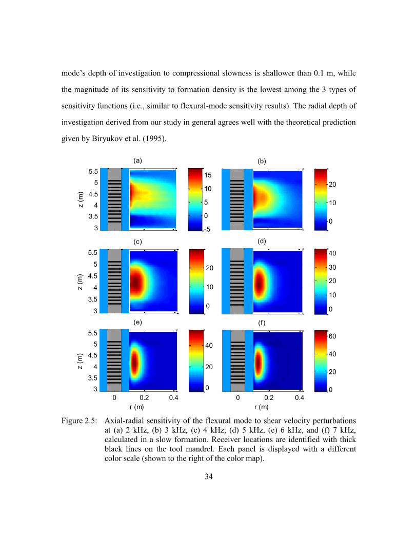
34
mode’s depth of investigation to compressional slowness is shallower than 0.1 m, while
the magnitude of its sensitivity to formation density is the lowest among the 3 types of
sensitivity functions (i.e., similar to flexural-mode sensitivity results). The radial depth of
investigation derived from our study in general agrees well with the theoretical prediction
given by Biryukov et al. (1995).
Figure 2.5: Axial-radial sensitivity of the flexural mode to shear velocity perturbations
at (a) 2 kHz, (b) 3 kHz, (c) 4 kHz, (d) 5 kHz, (e) 6 kHz, and (f) 7 kHz,
calculated in a slow formation. Receiver locations are identified with thick
black lines on the tool mandrel. Each panel is displayed with a different
color scale (shown to the right of the color map).
3
3.5
4
4.5
5
5.5
(a)
z (
m)
-5
0
5
10
15
(b)
0
10
20
3
3.5
4
4.5
5
5.5
(c)
z (
m)
0
10
20
(d)
0
10
20
30
40
0 0.2 0.4
3
3.5
4
4.5
5
5.5
(e)
r (m)
z (
m)
0
20
40
0 0.2 0.4
(f)
r (m)
0
20
40
60

35
Figure 2.6: (a) Axial sensitivity curves and (b) radial sensitivity curves obtained from
axial-radial sensitivity functions. Receiver locations are identified with thick
black lines on the tool mandrel.

36
Figure 2.7: Axial-radial sensitivity of the flexural mode to shear velocity perturbations
at 2 kHz, calculated from the transmitter to the top receiver. Receiver
locations are identified with thick black lines on the tool mandrel.
0 0.2 0.4 0.6 0.8 10
0.5
1
1.5
2
2.5
3
3.5
4
4.5
5
5.5
r (m)
z (
m)
-2
0
2
4
6
8
10
12
14

37
Figure 2.8: Flexural mode axial-radial sensitivities to compressional slowness
perturbations at (a) 3 kHz, (b) 5 kHz, and (c) 7 kHz. Flexural mode axial-
radial sensitivities to density perturbation at (d) 3 kHz, (e) 5 kHz, and (f) 7
kHz. Receiver locations are identified with thick black lines on the tool
mandrel. Each panel is displayed with a different color scale (shown to the
right of the color map).
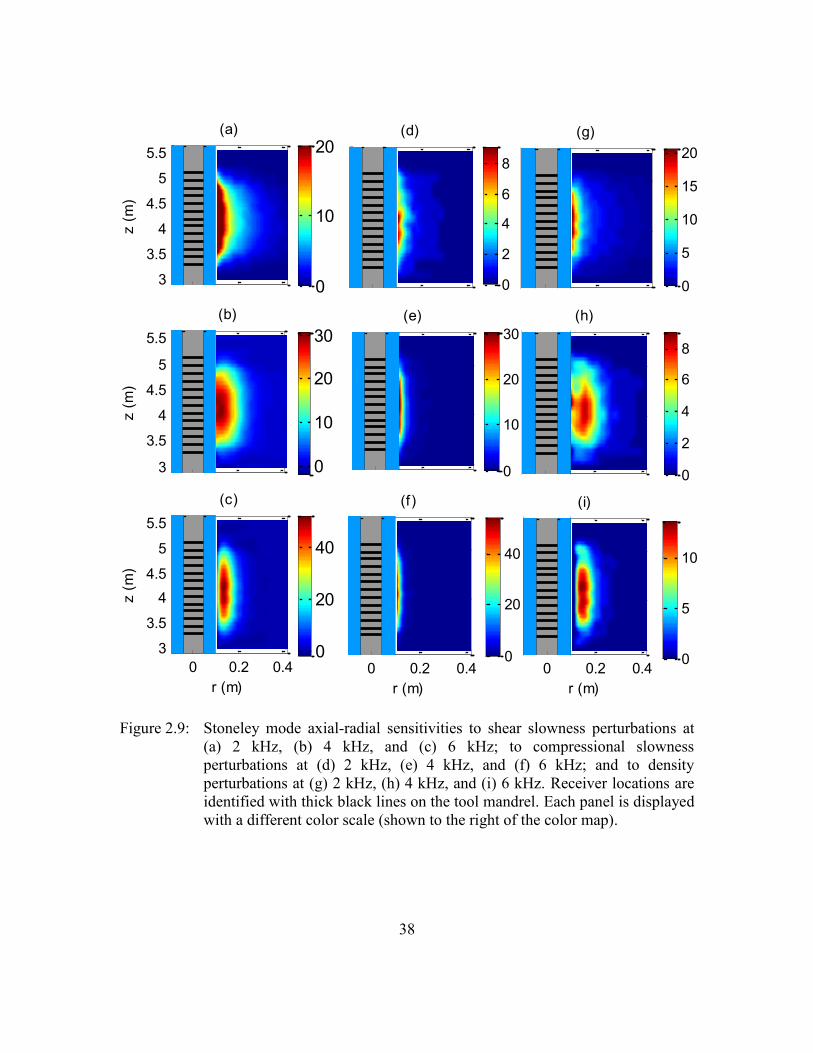
38
Figure 2.9: Stoneley mode axial-radial sensitivities to shear slowness perturbations at
(a) 2 kHz, (b) 4 kHz, and (c) 6 kHz; to compressional slowness
perturbations at (d) 2 kHz, (e) 4 kHz, and (f) 6 kHz; and to density
perturbations at (g) 2 kHz, (h) 4 kHz, and (i) 6 kHz. Receiver locations are
identified with thick black lines on the tool mandrel. Each panel is displayed
with a different color scale (shown to the right of the color map).
3
3.5
4
4.5
5
5.5
(a)z (
m)
3
3.5
4
4.5
5
5.5
(b)
z (
m)
0 0.2 0.4
3
3.5
4
4.5
5
5.5
(c)
r (m)
z (
m)
(g)
0
5
10
15
20
(h)
0
2
4
6
8
0 0.2 0.4
(i)
r (m)
0
5
10
(d)
0
2
4
6
8
(e)
0
10
20
30
0 0.2 0.4
(f)
r (m)
0
20
40
0
10
20
30
0
20
40
0
10
20

39
2.5 SEMI-ANALYTICAL AXIAL SENSITIVITY FUNCTIONS
In previous sections, we described 1D and 2D sensitivity functions calculated
with FE simulations. In order to calculate a particular type of sensitivity function, the
number of models needed to be simulated approximately equals the number of
perturbation cells. Furthermore, as a result of the errors associated with simulation and
dispersion processing, the sensitivity functions may suffer from instability, especially
when the sensitivity value is low. We now introduce an alternative semi-analytical
approach that delivers stable sensitivity curves and requires only two runs of numerical
simulations.
Axial sensitivity functions are calculated by modeling semi-analytically the
perturbation due to slowness variations. Owing to the introduction of perturbed layers
between consecutive receivers, we need to describe the modal wave propagation through
horizontally layered media in the presence of a fluid-filled wellbore. Gelinsky and Tang
(1997) developed a fast forward method for modeling Stoneley-wave propagation in
heterogeneous horizontally layered formations; predictive modeling of flexural waves
remains challenging. Instead of time-domain modeling, we describe a modal wave
spectrum, X, acquired at an arbitrary receiver, n, and a particular frequency, f, as
1n
nX f hz , (2.5)
where h is mode amplitude, and z stands for phase delay across the receiver array,
expressed as
2 ri fs dZ e , (2.6)
where sr is the phase slowness of the modal wave at f, and d equals the inter-receiver
spacing. Equations 2.5 and 2.6 state the fact that when a particular mode propagates
across the receiver array in a homogeneous formation, the phase difference between any
two consecutive receivers is a constant governed by the modal slowness. After

40
introduction of a thin layer with an elastic perturbation between receivers m and m+1, the
resulting spectrum at all receivers becomes
1 1
1 1, , , , , , TT m m i d s N i d s
NX f X f h Z Z Z e Z e , (2.7)
where N is the total number of receivers, and Δs is the variation in modal slowness at
2 f due to the elastic property perturbation.
Equation 2.7 allows us to approximate the measured spectrum without invoking
boundary conditions between borehole and formation, provided that we know sr and Δs.
We resort to numerical simulation (or any analytical dispersion estimation method) to
obtain sr and Δs. First, we simulate the dispersion curve in the homogeneous reference
medium (referred to as Mr in equation 2.2) and record s
r at f. Secondly, we simulate the
dispersion in a fully perturbed homogeneous formation (referred to as M in equation 2.2),
and obtain Δs at f. Because the two simulations are obtained for a fluid-filled borehole
and a rigid logging tool, the two sets of dispersion data intrinsically bear the influences of
borehole fluid, logging tool, and multiple horizontal boundaries. Figure 2.10 shows an
example of simulated dispersions in the slow formation described in Table 2.1, from
which we obtain sr, and Δs, and consequently the predicted spectrum. The next step is
slowness estimation using the WSS method, which has fundamentally the same
assumption as equation 2.6 wherein one maximizes the spectral semblance function,
defined as
* 1
0
1
0
*
1
, ,
Nn
n
n
N
n n
n
X f Z
f s
N X f X f
(2.8)
where * denotes complex conjugation, 0 0exp 2 εZ i fs d , 0s is the estimated
slowness, and ε is the error term. From equations 2.7 and 2.8, we observe that if, at each

41
receiver, 1
0
nZ is in phase with nX , then the numerator (hence the semblance) is
maximized. Therefore, the method is essentially a linear regression process given by
0
1 1
2 11 1
2 11
1 0 ε /1 1
0 11 0
0 0
r
N
NN
Nm s s
d dm s d
, (2.9)
where ε is the error term, and 0s is the estimated slowness. Equation 2.9 describes
a least-squares problem, with the solution given by
0 2
2
6
1
1 3ε
1
r
m N ms s s
N N
N m N ms
N N
. (2.10)
From the above equation, one infers that the estimated slowness, 0s , is well defined as
a linear function of sr and Δs. We also infer that the thickness of the perturbed layer, d,
does not contribute to the final expression for 0s , indicating that ideally the sensitivity
function should be a function of the elastic properties only, independent of perturbation
geometry. Additionally, the relative error in 0s is controlled by the perturbation ratio
Δs/sr.
Furthermore, although under perturbation conditions, reflection at a layer boundary is
one order of magnitude less than the incident signal, it may still introduce slight phase
changes; accordingly, we modify the approach by considering both up-going and down-
going waves in the perturbed layer and in the formations below it. As shown in Figure

42
2.11, it then follows that one has a total of 5 waves propagating in the layered formation.
For up-going source direct radiation, we set its amplitude (denoted by A in Figure 2.11)
equal to one, whereupon there are four unknown complex amplitudes, which can be
solved using displacement and stress continuity conditions across the boundaries, as
1' '
2 2' '2 2
' '
2 2' ' 2
e 'e 'e 0 e
e ' ' e ' ' e 0 e
0 'e 'e e 0
00 ' ' e ' ' e e
L L LL
L L L L
U U U
U U U
ikz ik z ik zikz
ikz ik z ik z ikz
ik z ik z ikz
ik z ik z ikz
k k kB k
C Lk L k L k Lk
D k k k
E L k L k Lk
, (2.11)
where k and k’ are the wavenumbers according to sr and s
r+Δs, respectively, and L and
L’ are the equivalent moduli defined as
2 2 2 2
22 2 2
4 / ,
' ' 4 / ' ,
L c f k
L c f k
(2.12)
where, Lz and Uz are the lower and upper boundary locations of the perturbed layer,
respectively, and ρ is density. Because the reflected signals are weaker than the
transmitted ones, we neglect B and D to obtain the spectrum as
1 1 1'
1 , , 1, , , , , , ,TT ik m d ik m d ik N dikd ik md
NX f X f e e Ce Ee Ee
,
(2.13)
where we vary m from 1 to N-1 for perturbation analysis, following the same procedure
implemented with FE simulations.
We calculate axial sensitivity functions in the slow formation (given in Table 2.1)
for the flexural mode, and show the results in Figure 2.12. In comparison to the
numerically calculated curves shown in Figure 2.2, we observe that the semi-analytical
sensitivity functions properly describe the magnitude and frequency dependence of the
numerical results. Additionally, the semi-analytical results have better stability than those

43
obtained with numerical simulations. Figure 2.13 shows another set of example
sensitivity functions calculated with the Stoneley mode in the slow formation (given in
Table 2.1), which compares well to the numerical results displayed in Figure 2.4.
Figure 2.10: Slowness dispersions calculated in the reference medium (circles)
and in the fully perturbed formation (crosses).
Figure 2.11: Wave potentials propagating in the effective layered medium.

44
Figure 2.12: Semi-analytical sensitivity functions of the flexural mode to (a) shear
slowness, (b) compressional slowness, and (c) density perturbations
calculated for the slow formation. Receiver locations are identified with
thick black lines on the tool mandrel.

45
Figure 2.13: Semi-analytical sensitivity functions of the Stoneley mode to (a) shear
slowness, (b) compressional slowness, and (c) density perturbations
calculated for the slow formation. Receiver locations are identified with
thick black lines on the tool mandrel.

46
Figure 2.14: Radial sensitivity functions of the flexural mode to (a) shear slowness, (b)
compressional slowness, and (c) density perturbations calculated for the
slow formation.

47
2.6 SEMI-ANALYTICAL AXIAL-RADIAL SENSITIVITY FUNCTIONS
The calculation of 2D axial-radial sensitivity maps follows as a straightforward
extension of 1D axial sensitivity functions. It can be described as the tensor product
, ,
,
,
, , , ,, , ,
, ,
a z r a r r
a r z r
a r rr
G z M f G r M fG r z M f
G r M f rdr
, (2.14)
where ,a zG is the semi-analytical axial sensitivity, ,a rG is the radial sensitivity functions,
,a r zG is the 2D sensitivity map, and the symbol represents tensor product. Radial
sensitivity functions, ,a rG , are calculated by introducing concentric cylindrical
perturbation layers in the radial direction. For each perturbation, slowness dispersion is
obtained by solving the dispersion equation, which is constructed by enforcing continuity
conditions at cylindrical radial layer boundaries (Tang et al., 1999). Figure 2.14 shows a
set of radial sensitivity curves calculated for the slow formation described in Table 2.1.
According to equation 2.14, using the radial and axial sensitivity functions shown
in Figures 2.12 and 2.14, we approximate flexural-mode 2D sensitivity maps displayed in
Figure 2.15 due to perturbations of shear slowness. In general, the semi-analytical maps
predict well the flexural mode propagation properties. As frequency increases from 2 to 7
kHz, the sensitivity maps contract significantly toward the borehole wall, which reflects
the frequency dependence of the radial length of investigation for the flexural mode. In
the vertical direction, the sensitivity map at each frequency is symmetric about the center
receiver, indicating that rock formations closer to the central receiver are responsible for
the largest contribution to the dispersion measurement. Additionally, the integration of
each sensitivity map is a constant as a result of the normalization implemented in the
calculation of the sensitivity function.
Figure 2.16 displays the semi-analytical sensitivity maps calculated for
compressional slowness and density perturbations, which represent the ones shown in

48
Figure 2.8. The semi-analytical sensitivity maps exhibit better stability than the ones
obtained using numerical perturbation analysis. Figure 2.17 shows the Stoneley-mode
semi-analytical sensitivity maps calculated following the same workflow as the flexural
mode. The maps agree well to the corresponding ones shown in Figure 2.9 in terms of
investigation depth and sensitivity magnitude.

49
Figure 2.15: Semi-analytical axial-radial sensitivity of the flexural mode to shear velocity
perturbations at (a) 2 kHz, (b) 3 kHz, (c) 4 kHz, (d) 5 kHz, (e) 6 kHz, and (f)
7 kHz, calculated in the slow formation. Receiver locations are identified
with thick black lines on the tool mandrel. Each panel is displayed with a
different color scale (shown to the right of the color map).
3
3.5
4
4.5
5
5.5
(a)z (
m)
2
4
6
8
10
12
(b)
5
10
15
20
3
3.5
4
4.5
5
5.5
(c)
z (
m)
10
20
30
(d)
0
10
20
30
40
0 0.2 0.43
3.5
4
4.5
5
5.5
(e)
r (m)
z (
m)
0
20
40
60
0 0.2 0.4
(f)
r (m)
0
20
40
60

50
Figure 2.16: Semi-analytical axial-radial sensitivity of the flexural mode to
compressional slowness perturbation at (a) 3 kHz, (b) 5 kHz, and (c) 7 kHz,
and to density perturbation at (d) 3 kHz, (e) 5 kHz, and (f) 7 kHz. Each
panel is displayed with a different color scale (shown to the right of the
color map).
3
3.5
4
4.5
5
5.5(a)
z (
m)
0
5
10
3
3.5
4
4.5
5
5.5(b)
z (
m)
10
20
30
0 0.2 0.43
3.5
4
4.5
5
5.5(c)
r (m)
z (
m)
0
10
20
30
40
3
3.5
4
4.5
5
5.5(d)
0
1
2
3
3.5
4
4.5
5
5.5(e)
2
4
6
8
10
0 0.2 0.43
4
5
(f)
r (m)
z (
m)
0
5
10
15

51
Figure 2.17: Semi-analytical axial-radial sensitivity of the Stoneley mode to shear
slowness perturbation at (a) 2 kHz, (b) 4 kHz, and (c) 6 kHz, to
compressional slowness perturbation at (d) 2 kHz, (e) 4 kHz, and (f) 6 kHz,
and to density perturbation at (g) 2 kHz, (h) 4 kHz, and (i) 6 kHz. Each
panel is displayed with a different color scale (shown to the right of the
color map).
3
3.5
4
4.5
5
5.5(a)
z (
m)
0
10
20
3
3.5
4
4.5
5
5.5(b)
z (
m)
0
10
20
30
0 0.2 0.43
3.5
4
4.5
5
5.5(c)
r (m)
z (
m)
0
20
40
(d)
0
2
4
6
8
10
(e)
0
10
20
30
0 0.2 0.4
(f)
r (m)
0
10
20
30
40
(g)
0
5
10
15
20
(h)
0
5
10
0 0.2 0.4
(i)
r (m)
0
5
10
15

52
2.7 AXIAL SENSITIVITY FUNCTIONS OF NON-DISPERSIVE MODES
In addition to the dispersive mode measurements, compressional- and shear-mode
slowness logs are two of the fundamental sonic logging products used for assessing
petrophysical and mechanical properties of rock formations. Compared to dispersive
modes, the compressional (in all types of formations) and shear modes (in fast
formations) show negligible dispersion with respect to frequency. Additionally, unlike
dispersive modes whose slownesses are influenced by multiple formation properties, the
non-dispersive compressional- and shear-mode slownesses are chiefly controlled by the
compressional and shear slownesses of the rock formation, respectively. Such
characteristics of these 2 modes enable us to extend the 1D axial sensitivity functions to
rapidly model compressional- and shear-mode slowness logs in formations with thin
beds.
As the flexural-mode sensitivity analysis shows, formation shear slowness
dominantly controls the propagation of the flexural mode at low frequencies, whereby the
low-frequency asymptote of the flexural mode is often used to estimate formation shear
slowness. Consequently, we can apply the same procedure as for the flexural mode to
calculate the sensitivity function of the shear mode. Because the shear mode is only
sensitive to formation shear slowness, the variation in shear-mode slowness is equal to
the perturbation in formation shear slowness. Accordingly, equation 2.10 can be
simplified as
0 2
6
1r r
m N ms M M M
N N
, (2.15)
where Mr and M are the reference and perturbed formation shear slownesses,
respectively. Substitution of equation 2.15 into the definition given in equation 2.2 yields

53
, 2
6
1a z
m z N m zG z
N N
, (2.16)
where we notice that the sensitivity, Ga,z, is a function of z only, independent of both
perturbation amount and elastic properties of the reference medium. Applying the layered
formation approximation shown in Figure 2.11, we obtain the axial sensitivity function
for the shear mode shown in Figure 2.18. In general, the sensitivity function is a bell-
shaped curve symmetric about the mid-point of the receiver array. The sensitivity
approaches zero below and above the bottom receivers, respectively, which is in
agreement with the measurement physics.
Compressional-mode slowness is often estimated with the slowness-time
coherence (STC) method (Kimball and Marzetta, 1986). The method is based on the
semblance of the waveforms across the receiver array, similar to the spectrum semblance
method for deriving the dispersive-mode sensitivity functions. Furthermore, analogous to
the shear mode, the propagation of the compressional mode only depends on the
compressional slowness of the formation, hence we are able to apply the same sensitivity
curve shown in Figure 2.18 to model compressional slowness logs in thinly bedded
formations.

54
Figure 2.18: Semi-analytical axial sensitivity function for the compressional and shear
modes. Receiver locations are identified with thick black lines on the tool
mandrel.

55
2.8 MODELING DISPERSION IN THIN BEDS
This section documents synthetic examples used to benchmark the modeling of
sonic slowness dispersions using axial sensitivity functions. Escalation of error and the
strategy to control it are also discussed in the section.
In the first example, we model dispersions measured along a transition interval
from a fast formation at the bottom to a slower formation at the top, which also includes
two thin beds in the middle. Detailed formation properties are listed in Table 2.3. This
synthetic example represents typical layered formations resulting from consolidation and
changes in sedimentary environments. The transition between the bottom and top
formations is characterized by a gradual decrease in rock density and elastic properties.
Because the well is drilled vertically, rock formations in the proximity of the borehole
exhibit property variations only in the vertical direction, which allows us to use 1D axial
sensitivity functions to calculate sonic dispersions. Differences in elastic properties and
density for each layer are regarded as perturbations from the reference medium, and we
simulate dispersion using semi-analytical axial sensitivity functions given by
, , ,r
r a z r
M z r
M zs f s f G z M f z
M
, (2.17)
where the first sum loops across all 3 formation elastic properties, and ∆M denotes the
perturbation of a particular property. Equation 2.17 is a 1D discrete expression of integral
equation 2.1, which defines the sensitivity function.
Table 2.3 lists the assumed model properties; the fast formation described in
Table 2.1 serves as the reference medium in the calculations. A wireline dipole tool
operates across the transition interval.
Figure 2.19(a) displays the slowness logs obtained with the semi-analytical
sensitivity functions at six discrete frequencies, which show good agreement with the

56
results obtained with FE calculations. Additionally, because the new method models
dispersion by means of integration, not via solving wave equations numerically, it
significantly reduces the associated CPU time from two hours to less than one minute on
a quad-core PC processor.
Figure 2.19(b) displays the Stoneley-mode slowness log modeled using the semi-
analytical axial sensitivity functions shown in Figure 2.13. Because high frequency part
of Stoneley mode is dominantly controlled by borehole fluid, we are more interested in
modeling its low frequency components. In addition, as Stoneley mode is less dispersive,
only 1-kHz component is plotted for comparison. Obviously, the modeled log agrees well
to the simulated one.
To model a slowness log, equation 2.17 needs to be applied across the entire
logging interval. When formation properties significantly differ from the properties of the
reference formation, the modeling error often increases. To reduce the error, we select the
sensitivity functions adaptively, which is discussed in the next example.
In previous sections, we described slowness sensitivity functions based on
perturbation analysis. Because the calculated sensitivity functions are associated with the
elastic properties of the reference formation, the modeled logs are only correct (self
consistent) if the differences between the elastic properties of the modeled (M in equation
2.2) and reference formation (Mr in equation 2.2) are within the perturbation limit.
To this end, we study the propagation of numerical errors using an example when
the tool penetrates multiple thin beds. The formation consists of eight thin beds with
uniform thickness of 3 ft. Layer elastic properties exhibit large variations, plotted in
Figure 2.20 as blocky profiles. Figure 2.21 also shows the shear slowness, compressional
slowness, and density logs obtained from FE numerical simulations, from which we
select reference formations.

57
We first use a single reference formation by spatially averaging the logs along the
entire depth interval. The calculations of shear and compressional slowness are
implemented by averaging the moduli λ and μ, which ensures self-consistent reference
values for slownesses. Figure 2.21 shows the properties of the resulting reference
formation as vertical solid lines, which are input into equation 2.2 to calculate the
sensitivity functions. From the calculated sensitivity functions, the flexural and Stoneley
dispersion logs are modeled using equation 2.17. In Figure 2.22, we notice that for both
modes, the modeled logs (circles) best match the simulated ones (solid) from 4.5 to 6.5
m, where the differences between the elastic properties of the layers and those of the
reference formation are within the perturbation limit. To assess the accuracy of the rapid
simulation method, we also calculate the relative error, defined as the slowness difference
between the modeled and numerically simulated logs normalized by the slowness value
obtained from numerical simulation. Figure 2.23 shows the relative errors at the lowest
frequencies (2 kHz for the flexural mode and 1 kHz for the Stoneley mode) as triangles,
from which we observe a systematic increase of errors.
To reduce the error, we select the reference formations adaptively using a test
averaging window on the shear slowness log. The window begins at the first depth and
extends toward deeper depths. As the window lengthens, we calculate an average shear
slowness value from all depths included in the window. Next, the log value at each depth
is compared to the average value. Once the slowness difference at a particular depth
exceeds 15% with respect to the average, the window is cut and a new window begins at
the next depth. The compressional slowness references are calculated following the same
procedure that averages λ and μ. As shown in Figure 2.24, by applying the new approach,
seven different reference formations are chosen as local background. Because the density
sensitivity is low and the density log exhibits very slight variations, we still use a single

58
density value as reference. Figure 2.25 compares the dispersion logs; we observe that the
sensitivity-modeled logs agree well with the ones obtained with FE simulations. The
relative errors also significantly decrease to values lower than 3%, as indicated by the
circles in Figure 2.23.
We further refine the selection of reference formations at depths from 4 to 7 m.
From the refinement, nine reference formations are selected. Figure 2.26(a) shows the
shear slowness values of the reference formations. Based on the error comparison in
Figure 2.26(b), we conclude that there is an intrinsic error of 2% associated with the new
simulation method, and the adaptive adjustment of reference formations helps to lower
the error to that intrinsic level.
Table 2.3: Assumed layer properties.
Δz (m) pv (m/s) sv (m/s) ρ (kg/m
3)
Top ∞ 3083 1710 1980
Layer 1 0.52 3464 1940 2112
Layer 2 0.55 3643 2095 2330
Bottom ∞ 3845 2200 2860

59
Figure 2.19: (a) Comparison of flexural dispersion logs calculated with the sensitivity
method (circles) and finite-element numerical simulations (solid), and (b)
comparison of the Stoneley dispersion logs at 1 kHz obtained with the
sensitivity method (circles) and numerical simulations (solid).

60
Figure 2.20: Vertical distributions of (a) shear slowness, (b) compressional slowness, and
(c) density.

61
Figure 2.21: (a) Shear slowness log, (b) compressional slowness log, and (c) density log.
The solid line on each subplot describes the reference formation property.

62
Figure 2.22: (a) Comparison of flexural dispersion logs calculated with the sensitivity
method (circles) and numerical simulations (solid), and (b) comparison of
Stoneley dispersion logs calculated with the sensitivity method (circles) and
numerical simulations (solid). The reference formation shown in Figure 2.23
is used for sensitivity calculations.
0
5
10
100150200250300
z (
m)
(a)
Slow ness (us/ft)
0
2
4
6
8
10
200220240260280300
Slow ness (us/ft)
(b)
z (
m)
2 kHz
4 kHz
6 kHz
1 kHz
3 kHz
5 kHz
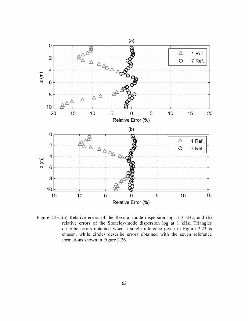
63
Figure 2.23: (a) Relative errors of the flexural-mode dispersion log at 2 kHz, and (b)
relative errors of the Stoneley-mode dispersion log at 1 kHz. Triangles
describe errors obtained when a single reference given in Figure 2.23 is
chosen, while circles describe errors obtained with the seven reference
formations shown in Figure 2.26.

64
Figure 2.24: (a) Seven reference values are adaptively selected based on the shear
slowness log, (b) seven compressional slowness reference values are
adaptively selected according to the shear slowness references, and (c) the
density reference value.

65
Figure 2.25: (a) Comparison of flexural dispersion logs calculated with the sensitivity
method (circles) and numerical simulations (solid), and (b) comparison of
Stoneley dispersion logs calculated with the sensitivity method (circles) and
finite-element numerical simulations (solid). The reference formations
shown in Figure 2.26 were used for sensitivity calculations.
200220240260280300
0
2
4
6
8
10
z (
m)
Slow ness (us/ft)
(b)1 kHz
3 kHz
5 kHz
0
2
4
6
8
10100150200250300
Depth
(m
)
Slow ness (us/ft)
(a)
2 kHz
4 kHz
5 kHz
6 kHz
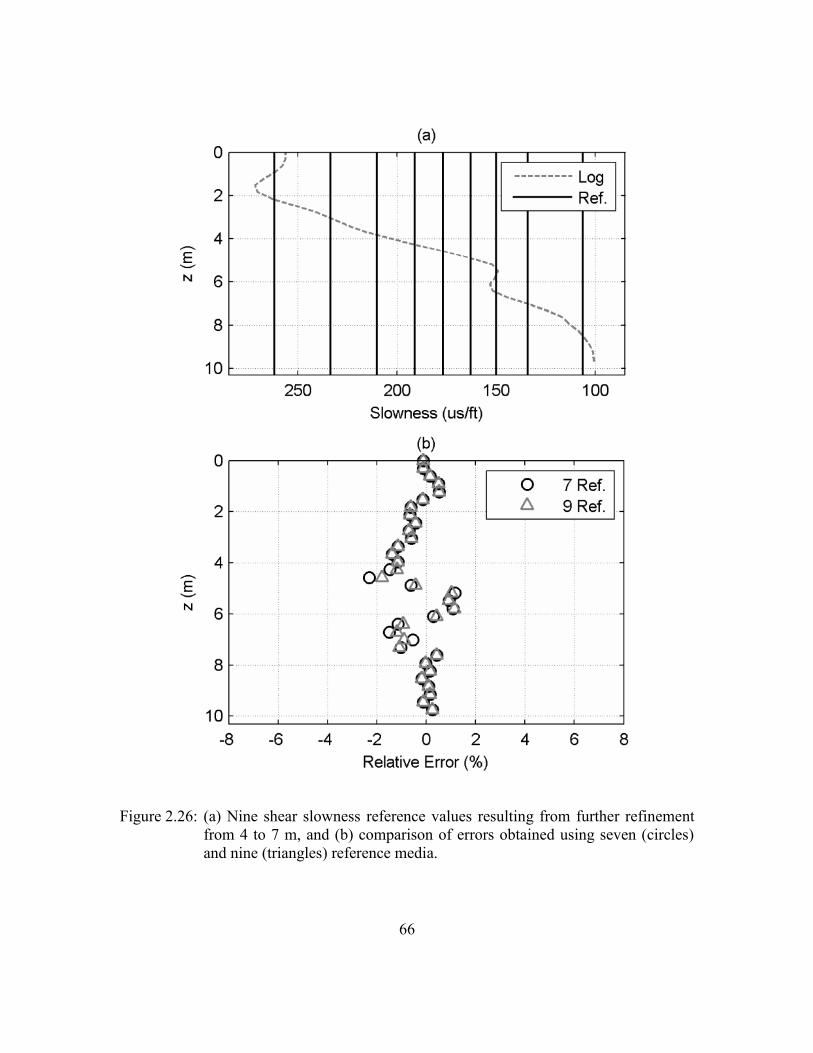
66
Figure 2.26: (a) Nine shear slowness reference values resulting from further refinement
from 4 to 7 m, and (b) comparison of errors obtained using seven (circles)
and nine (triangles) reference media.

67
2.9 MODELING DISPERSION IN THIN BEDS WITH INVASION
In this section, we examine another synthetic example when the tool logs across
rock formations with horizontal thin beds. In addition to elastic property variations along
the borehole axis, mud-filtrate invasion in two thin beds gives rise to radially varying
fluid saturations. Such saturation profiles impact density and velocities of the rock
formation (Han, 1992) and create multiple layers of radial alterations. Consequently, as
shown in Figure 2.27, there are nine types of formations with different properties. In
order to simulate modal wave dispersions, we invoke axial-radial sensitivity functions to
account for 2D elastic property variations. Table 2.4 summarizes the model parameters
calculated with a fluid substitution approach (Mavko et al., 2003). Borehole size, fluid
type, and logging instrument are the same as in Synthetic Example 1. We use the slow
formation described in Table 2.1 as the reference medium, and model the dispersions at
discrete frequencies using the semi-analytical axial-radial sensitivity functions with
regard to shear slowness, compressional slowness, and density perturbations. The
mathematical expression for fast modeling is readily derived from equation 2.4, as
,
,
,, , ,
r
r a r z r
M r z r
M r zs f s f G r z M f r r z
M
, (2.18)
which differs from equation 2.17 in the second sum, which loops through each
discretization in the axial and radial directions. Finally, we apply equation 2.18 at all
depths to calculate synthetic dispersion logs.
In Figure 2.28(a), we compare modeled sensitivity flexural mode dispersion logs
to logs simulated with the FE method. Across all depths and frequencies, modeled logs
show good agreement with those obtained from FE simulations. The maximum absolute
error for the flexural mode takes places at 2.75 m with the 2 kHz slowness log, which
equals 3.1 us/ft, with the maximum relative error equal to 1.2%. Although the semi-

68
analytical sensitivity map at 2 kHz does not completely reproduce the tubular shaped map
shown in Figure 2.7, it does capture the concentrated sensitivity about the receiver array,
and consequently the estimated log agrees well with the one obtained with FE simulation.
Likewise, the accuracy of the calculated Stoneley-mode slowness is comparable to that of
the flexural mode. In Figure 2.28(b), the maximum absolute error equals 2.5 us/ft at 1.07
m, equivalent to 1% relative error.
Figure 2.27: Geometry of the formation with invaded thin beds. Receiver locations are
identified with thick black lines on the tool mandrel.

69
Figure 2.28: (a) Comparison of the flexural dispersion logs calculated with the sensitivity
method (circles) and finite-element numerical simulations (solid); (b)
comparison of the Stoneley dispersion logs calculated with the sensitivity
method (circles) and finite-element numerical simulations (solid). Only the
logs at 1 kHz are shown for comparison because the Stoneley mode is less
dispersive than the flexural mode.

70
Table 2.4: Properties assumed for the rock formation with invaded thin beds.
Index Δr (m) pv (m/s) sv (m/s) ρ (kg/m
3)
1 ∞ 2550 1350 2075
2 0.05 2380 1180 2000
3 0.025 2310 1190 1925
4 0.05 2205 1230 1830
5 ∞ 2250 1245 1790
6 0.05 2400 1170 2040
7 0.1 2290 1225 1900
8 0.075 2275 1230 1865
9 ∞ 2265 1255 1810

71
2.10 MODELING NON-DISPERSIVE MODE SLOWNESS LOGS
We implement the sensitivity curve shown in Figure 2.18 on 3 synthetic cases
which include thin beds and large contrasts in shear and compressional slownesses. Table
2.5 lists the assumed properties for the 3 cases, where layers 1 and 5 are the shallowest
and deepest layers, respectively. The model properties are input into FE and finite-
difference simulations to calculate frequency spectra and waveforms, respectively.
Because all models include slow formations, we derive shear slowness logs from the
simulated flexural mode spectra. Simultaneously, we calculate compressional slowness
logs by processing the waveforms with the STC method.
The formation model 1 includes a slow and a fast layer embedded in a
homogeneous background. Because the thicknesses of layers 2, 3, and 4 are less than half
the axial length of the receiver array, we expect the logs to exhibit spatially averaged
slowness values, governed by the measurement sensitivity along the axial direction. In
Figure 2.30, we show the slowness logs calculated with the sensitivity curve, compared to
those obtained with numerical simulations. Firstly, we notice that the modeled logs agree
well with the simulated ones, with maximum relative errors of 2.1% and 2.6% for
compressional and shear modes, respectively. Secondly, we compare the logs to the
model parameters (described with the blocky profile), and find that the sensitivity
modeling method correctly reproduces the spatial averaging effect due to the receiver
array. At the center of layer 4, the maximum relative difference between the log and the
model (layer) properties equals 14.4% and 14.7% for the compressional and shear modes,
respectively. These results indicate that shoulder-bed effects on sonic logs can bias their
interpretation.
In formation model 2, the thin beds 2, 3, and 4 are unevenly shouldered by layers
with different elastic properties. The model also includes thin beds with large slowness

72
contrasts. Layers 2 and 3 exhibit a compressional slowness difference of 60 us/ft, and a
shear slowness contrast over 80 us/ft. Figure 2.31 compares the modeled and numerically
simulated logs. The maximum relative errors equal 2.2% and 3% for compressional and
shear slowness, respectively. When comparing the logs to the original model, we observe
10% and 12% relative differences for compressional and shear slownesses, respectively.
Sub-array processing techniques are often used to enhance the resolution of sonic
logs (Hsu and Chang, 1987; Zhang et al., 2000). The fast simulation method introduced
in this paper is also applicable to model sonic logs obtained with sub-arrays.
Accordingly, the semi-analytical formulation given by equation 2.18 can be used to
describe the sensitivity function of a given sonic sub-array by adjusting the parameter N
that designates the total number of receivers assigned to the sub-array. In formation
model 2, numerically simulated waveforms from receivers 4 to 10, 5 to 9, and 6 to 8
(which correspond to ½, ⅓, and ¼ of the whole array, respectively) are processed to
obtain slowness logs. We keep receiver 7 as the center of the sub-arrays such that no
depth shift is introduced in the study. Figure 2.32 shows sonic logs obtained from fast-
forward modeling and rigorous numerical simulations, while panels 2.32(a) to 2.32(d) in
the same figure describe results obtained with the complete receiver array , ½-, ⅓-, and
¼-length sub-arrays. Sonic logs numerically simulated with a shorter receiver array show
higher semblance with the original slowness model, which verifies the enhancement in
vertical resolution. However, it is important to point out that a decrease in the number of
receivers used in the calculation of slownesses gives rise to “noisy” sonic logs obtained
with rigorous waveform simulations when compared to those calculated across the entire
receiver array. This behavior occurs because the stability and reliability of slowness-
processing methods decreases with a decrease in the number of receivers. Sonic logs
obtained with rigorous numerical simulations and shown in Figure 2.32(d) contain

73
irregular vertical variations while the logs simulated with sensitivity functions are
consistently smooth and closely track the original model. This exercise confirms that the
sonic sensitivity method can be used in conjunction with sub-array processing techniques
to provide stable high-resolution interpretations of sonic logs.
Model 3 consists of three thin beds embedded in a homogeneous background
formation. Layers 2 and 4 are slower than the background medium whereas layer 3 is
significantly faster than the background. Figure 2.33 shows the sonic logs calculated with
fast forward modeling and numerical simulations, where we observe 2.7% and 3.6%
maximum relative errors for compressional and shear slowness, respectively. In contrast
to previous models, we also observe that the two slower peaks (at depths 1.22 m and 3.66
m) on the logs do not correspond to the mid points of layers 2 and 4 (at depths 1.46 m
and 3.26 m). This “shifting” effect is caused by uneven shoulder-bed averaging; when the
tool operates across layer 2 and 4, the measured logs reflect a weighted spatial average
involving also the fast layer (layer 3). Therefore, the slowness peaks for layers 2 and 4
are offset by layer 3, which results in apparent biases of the peak locations. We therefore
conclude that bed boundaries not only impact the slownesses reported by sonic logs but
may also bias the assessment of true layer properties.
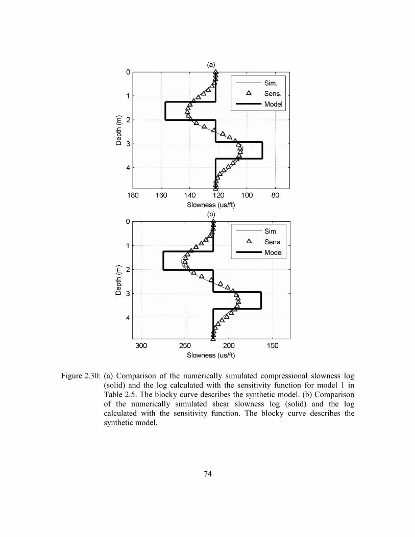
74
Figure 2.30: (a) Comparison of the numerically simulated compressional slowness log
(solid) and the log calculated with the sensitivity function for model 1 in
Table 2.5. The blocky curve describes the synthetic model. (b) Comparison
of the numerically simulated shear slowness log (solid) and the log
calculated with the sensitivity function. The blocky curve describes the
synthetic model.
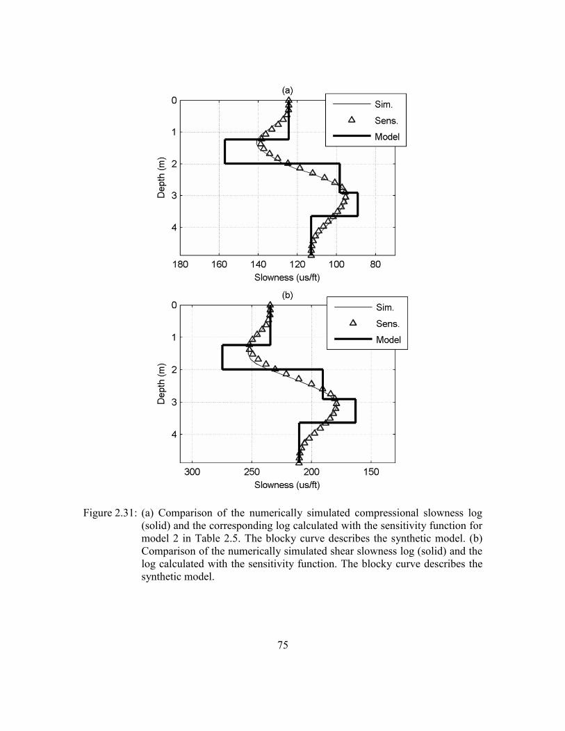
75
Figure 2.31: (a) Comparison of the numerically simulated compressional slowness log
(solid) and the corresponding log calculated with the sensitivity function for
model 2 in Table 2.5. The blocky curve describes the synthetic model. (b)
Comparison of the numerically simulated shear slowness log (solid) and the
log calculated with the sensitivity function. The blocky curve describes the
synthetic model.

76
Figure 2.32: Slowness logs obtained with rigorous numerical simulations and fast-
forward modeling compared to the model. In each panel, thick curves
identify logs obtained with rigorous numerical simulations while triangles
identify logs obtained with fast-forward modeling; blocky curves identify
the model; the curves in black and grey identify compressional and shear
slowness logs, respectively. Different panels show results obtained using (a)
receivers 1 to 13, (b) receivers 4 to 10, (c) receivers 5 to 9, and (d) receivers
6 to 8.

77
Figure 2.33: (a) Comparison of the numerically simulated compressional slowness log
(solid) and the log calculated with the sensitivity function for model 3 in
Table 2.5. The blocky profile describes the synthetic model. (b) Comparison
of the numerically simulated shear slowness log (solid) and the log
calculated with the sensitivity function. The blocky curve describes the
synthetic model.

78
Table 2.5: Properties assumed for the synthetic rock formations for shear and
compressional slowness modeling.
Formation Layer Δz (m) pv (m/s) sv (m/s) ρ (kg/m3)
1
1 ∞ 2500 1400 2580
2 0.762 1940 1110 2540
3 0.914 2500 1400 2580
4 0.701 3420 1870 2625
5 ∞ 2500 1400 2580
2
1 ∞ 2580 1300 2580
2 0.762 1940 1110 2540
3 0.914 3100 1600 2590
4 0.732 3420 1870 2625
5 ∞ 2700 1450 2600
3
1 ∞ 2960 1600 2650
2 0.792 2680 1440 2620
3 0.853 4190 2150 2710
4 0.792 2680 1440 2620
5 ∞ 2960 1600 2650

79
2.11 DISCUSSION
In all synthetic examples, the maximum relative errors of the logs calculated
using the rapid modeling method are below 4% with respect to the logs calculated with
FE or finite-difference numerical simulations. All calculations described in this chapter
were carried out with the same PC furbished a quad-core processor. It takes
approximately 3.9 hours of CPU time to complete the FE calculations at all depths, while
it takes approximately 5 minutes of CPU time for the sensitivity method to calculate the
same logs.
Experience shows that when deriving the sensitivity functions, the size of
slowness perturbations is controlled to be 20%, therefore, the method is valid if the
maximum layer slowness is less or equal to 150% of the minimum layer slowness in a
particular rock formation model. For formations exhibiting larger property variations,
multiple sets of sensitivity functions must be adaptively calculated to be in agreement
with the calculated shear slowness log. Another limitation is that the method is only
applicable to modal wave slowness in vertical wells. In high-angle wells with thin beds,
multiple normal modes are excited simultaneously. These modes interfere with each other
and cause significant mode splitting in dispersion analysis, which requires further study
of the associated wave propagation physics.
2.12 CONCLUSIONS
We introduced axial and axial-radial slowness spatial sensitivity functions to
describe and numerically simulate fundamental borehole acoustic modes using
perturbation analysis and FE calculations. Based on numerical results, we developed a
semi-analytical approach, which not only theoretically validates our perturbation method,
but also provides the means to efficiently calculate the sensitivity functions. It was found
that the sensitivity functions depend on 3 formation elastic properties (shear slowness,

80
compressional slowness, and density), frequency, wave mode, and geometry of the
receiver array. It was also found that for fundamental guided waves at low frequencies, a
perturbation in formation shear slowness has the largest influence on the propagation
characteristics, whereas at high frequencies both formation compressional slowness and
density can have a measurable effect. The sensitivity functions form the basis of a new
method for the rapid and accurate simulation of multiple-frequency borehole sonic
measurements. Using the semi-analytical approach, the sonic sensitivity functions were
adaptively calculated based on the shear slowness log; they function as spatial weighting
filters to estimate modal wave dispersions in the presence of spatial variations of
formation elastic properties. Using synthetic examples with thin beds and invasion, we
modeled multi-frequency dispersions of flexural and Stoneley modes, and obtained
accurate results with significant reduction in computation time compared to standard
numerical simulation methods. Additionally, we extended the sensitivity concept to the
rapid numerical simulation of non-dispersive compressional and shear modes; results
conclusively indicated that the method is accurate and reliable to numerically simulate
compressional and shear slowness logs acquired in thinly bedded formations. The new
rapid simulation method opens the possibility of quantitative integration of modern sonic
logs with other borehole measurements for inversion-based petrophysical and
geomechanical interpretations.
The spatial sensitivity method developed in this chapter is limited to reproducing
frequency-dependent slownesses of dispersive modes (and propagation slowness of non-
dispersive modes) in vertical wells. Benchmarking exercises on rock formations
exhibiting large contrasts in elastic properties indicated that the relative error of the rapid
sonic-log simulation method is equal or lower than 4%.

81
Chapter 3: Inversion-based interpretation of borehole sonic
measurements using semi-analytical spatial sensitivity functions
One of the major challenges in the interpretation of sonic logs is the presence of
bed-boundary (shoulder-bed) effects, which can reduce the accuracy of estimated elastic
properties due to spatial averaging caused by the sonic receiver array across thin beds. A
reliable approach to account for shoulder-bed effects in the interpretation of sonic logs is
the implementation of forward modeling and inversion techniques. However, the
computation time required to model the direct problem, namely wave propagation in the
borehole environment, often inhibits the usage of inversion approaches in sonic-log
interpretation. We introduce an efficient inversion-based interpretation method for the
estimation of in-situ rock formation elastic properties from sonic logs. The method
employs semi-analytical spatial sensitivity functions for fast forward modeling of sonic-
slowness logs and estimates formation elastic properties by iteratively matching the
available logs with numerical simulations. We first develop a workflow to estimate shear
slowness of thin beds from flexural mode dispersions measured at multiple discrete
frequencies. Next, we extend the method to estimate layer-by-layer compressional and
shear slownesses by combining the slowness logs of both the non-dispersive
compressional (P-) and shear (S-) modes. This new inversion-based interpretation method
is verified using data numerically simulated for synthetic rock formations consisting of
multiple thin beds exhibiting large contrasts in elastic properties. Sonic data acquired in
wells penetrating multiple horizontal thin beds are also used to appraise the inversion-
based interpretation in the estimation of formation compressional and shear slownesses.
Results confirm the efficiency and reliability of the new inversion-based interpretation
method to enhance the vertical resolution of sonic logs. Our inversion-based

82
interpretation method opens the possibility of integrating modern borehole acoustic
measurements with nuclear and resistivity logs for improved poro-elastic and
petrophysical interpretations.
3.1 INTRODUCTION
Sonic logs are routinely used by the oil and gas industry in combination with
seismic amplitude measurements to detect, delineate, and appraise hydrocarbon
reservoirs. For reserves estimation, sonic logs are often used to quantify petrophysical
and rock mechanical properties of laminated thin beds. Because the conventional sonic
processing method (Kimball and Marzetta, 1986) estimates formation compressional and
shear slownesses by stacking the waveforms across the entire receiver array, the vertical
resolution of sonic logs is chiefly controlled by tool aperture (i.e., length of the receiver
array) (Tang and Cheng, 2004). When bed thickness is shorter than tool aperture the
resulting sonic logs provide spatially averaged slownesses, which can mask true
formation elastic properties. Interpretation of sonic logs without accounting for thin-bed
averaging effects often results in biased estimations of formation properties (Peyret and
Torres-Verdín, 2006; Oyler et al., 2008).
Various processing techniques have been developed for spatial resolution
enhancement of sonic logs. The multi-shot semblance method (Hsu and Chang, 1987)
utilizes overlapping sub-arrays across the same depth interval and obtains logs with
vertical resolution equal to the sub-array aperture. Zhang et al. (2000) performed thin-
bed slowness analysis using redundant information in overlapping sub-arrays to estimate
formation acoustic slowness with improved accuracy and resolution. However, the
associated processing techniques require shorter sub-arrays and utilize fewer traces of the
83
acquired waveforms, thereby rendering the estimated formation properties more sensitive
to noise contamination.
Aside from processing schemes based on sonic sub-arrays, inversion-based
methods can provide reliable interpretations of formation properties because of their
explicit usage of the associated measurement response functions. Much has been reported
on the application of inversion-based techniques to estimate layer-by-layer petrophysical
properties from well logs. Liu et al. (2007) introduced a joint inversion algorithm that
combines density and resistivity logs for improved hydrocarbon reserves estimations in
clastic sedimentary sequences exhibiting multiple thin beds. Sanchez-Ramirez et al.
(2010) combined gamma-ray, density, and resistivity logs to perform joint inversion of
petrophysical properties in thinly bedded rock formations. Using logging-while-drilling
measurements, Ijasan et al. (2013) introduced an efficient layer-based inversion workflow
for accurate estimation of hydrocarbon pore volume in high-angle and horizontal wells.
Yang and Torres-Verdín (2013) developed joint stochastic inversion methods for nuclear
and resistivity logs to estimate mineral/fluid concentrations that honor well logs and core
data.
Inversion methods have also been applied for the interpretation of borehole sonic
measurements. Tang and Chunduru (1999) developed a method for simultaneous
inversion of anisotropic parameters from cross-dipole array waveforms using a simulated
annealing algorithm. Based on a sensitivity study, Tang and Cheng (2004) introduced an
approach to estimate horizontal shear velocity from the Stoneley wave spectrum. To
address heterogeneity in elastic properties due to mud-filtrate invasion or near wellbore
damage, Sinha (1997) studied the multi-frequency sensitivity of flexural dispersions
using a general perturbation analysis based on Hamilton’s principle. This analysis formed
the basis of a parameterized model that enabled the radial profiling of formation shear

84
slowness (Yang et al., 2011). Sinha et al. (2006) proposed the radial profiling of three
anisotropic formation shear moduli from both monopole Stoneley and cross-dipole sonic
data. Using the full waveform inversion method, Chi et al. (2004) assessed the effect of
mud-filtrate invasion on sonic logs and estimated the radial distributions of formation
compressional velocity, shear velocity, and bulk density. In vertical wells, inversion of
cross-dipole measurements also aids in the estimation of far-field tectonic stresses (Sinha
and Kostek, 1996; Tang et al., 1999). Mallan et al. (2009) performed joint inversion of
flexural and Stoneley dispersions, as well as array-induction apparent resistivity
measurements to estimate dry bulk and shear moduli, porosity, and water saturation in the
radial direction.
Previously published methods for inversion-based interpretation of sonic logs
were based on the assumption that the formation being measured remains homogeneous
in the axial (vertical) direction of the wellbore. In the presence of axial heterogeneity, i.e.,
the formation consists of horizontal thin beds in the vertical direction, the conventional
Thomson-Haskell method (Tubman, 1984) cannot be used to model sonic measurements;
instead, numerical simulation methods (Cheng et al., 1995; Matuszyk et al., 2012;
Matuszyk et al., 2013; Matuszyk et al., 2014) are required to describe sonic wave
propagation in the borehole environment. The computation time required by such
numerical methods often inhibits the development and usage of inversion-based
interpretations. Gelinsky and Tang (1997) developed a fast forward method for modeling
low-frequency Stoneley-wave propagation in heterogeneous horizontally layered
formations. Recently, Huang et al. (2013) introduced spatial sensitivity functions of
borehole modal wave measurements, which enabled a new explicit relationship between
thin-bed-induced elastic property perturbations and the associated perturbations in
borehole sonic measurements. Details about the spatial sensitivity functions and fast

85
forward modeling method developed by Huang et al. (2013) are provided in the
appendices of this paper.
Based on previously developed algorithms for the fast simulation of sonic logs, in
this paper we develop an efficient inversion-based interpretation method to improve the
estimation of in-situ elastic properties from sonic logs in formations consisting of
multiple horizontal thin beds. Two inversion algorithms are developed which estimate
formation elastic properties by minimizing the quadratic difference between available
sonic logs and their numerical simulations. Additionally, we add Gaussian noise to the
numerically simulated data (or to field data in field cases) and iteratively invoke the
inversion algorithms to quantify the uncertainty of estimated elastic properties.
The first algorithm uses flexural-mode dispersion logs at multiple discrete
frequencies to estimate formation shear slowness; it is applied to a noisy synthetic case
when a vertical well penetrates multiple horizontal thin beds. Shear slownesses are
estimated to within a few percent of true values, accompanied by low uncertainties
(2.6%). The algorithm also improves the vertical resolution of the original measurement
to approximately 0.5 m. Applications to noisy field data verify that the algorithm reduces
shoulder-bed effects and yields reliable estimates of formation shear slowness.
The second algorithm addresses the problem of simultaneous inversion of
compressional and shear slownesses. By combining P- and S-mode slowness logs, we
formulate the inversion algorithm in terms of elastic moduli to ensure that the estimated
elastic properties are self-consistent. Numerical tests on synthetic and field examples
confirm that the joint inversion method yields accurate estimates of compressional and
shear slownesses which are consistent with rock-physics constraints. In comparison to
the first algorithm, the joint inversion method saves more than 80% of CPU time at a
price of slightly increased uncertainty (from 2.6% to 6%). Based on the estimated

86
compressional and shear slownesses, related rock mechanical properties are also
estimated together with their uncertainty. It is found that Young’s modulus and other
dynamic moduli calculated from sonic slownesses exhibit low uncertainties, whereas
dynamic Poisson’s ratio exhibits moderate to high uncertainty.
Developments and results described in this paper suggest the possibility of
inversion-based petrophysical and geomechanical interpretations that integrate modern
sonic logs with resistivity, nuclear, and magnetic resonance logs.
3.2 ESITMATION OF FORMATION ELASTIC PROPERTIES FROM FLEXURAL
DISPERSION DATA
Spatial sensitivity functions for sonic logs quantitatively relate formation elastic
properties to measurements. Forward modeling of sonic logs using semi-analytically
calculated sensitivity functions saves 98% of computation time compared to numerical
simulations. Appendix A introduces the semi-analytical spatial sensitivity functions and
the subsequent fast forward modeling method. The new modeling method invoked here
meets the prerequisite for developing an efficient inversion method to estimate formation
elastic properties. We formulate the inversion as a regularized nonlinear least-squares
minimization problem, in which the Levenberg-Marquardt method (Hansen, 1998; Aster
et al., 2005) is employed to find a solution. Using sensitivity analysis, we use flexural
mode slowness dispersion data to estimate shear slowness of each layer in thinly bedded
formations. Accordingly, the nonlinear parameter estimation problem is implemented to
minimize the additive quadratic cost function given by
2 22
22 C m g m d m , (3.1)
where m is the model vector that contains shear slownesses of the layers, d is the
observed data vector (the measurement vector), i.e., measured multi-frequency flexural
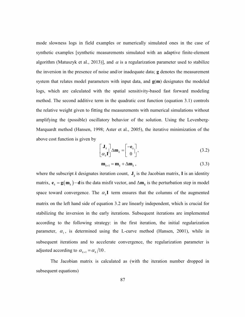
87
mode slowness logs in field examples or numerically simulated ones in the case of
synthetic examples [synthetic measurements simulated with an adaptive finite-element
algorithm (Matuszyk et al., 2013)], and is a regularization parameter used to stabilize
the inversion in the presence of noise and/or inadequate data; g denotes the measurement
system that relates model parameters with input data, and g(m) designates the modeled
logs, which are calculated with the spatial sensitivity-based fast forward modeling
method. The second additive term in the quadratic cost function (equation 3.1) controls
the relative weight given to fitting the measurements with numerical simulations without
amplifying the (possible) oscillatory behavior of the solution. Using the Levenberg-
Marquardt method (Hansen, 1998; Aster et al., 2005), the iterative minimization of the
above cost function is given by
0
J em
I
k k
k
k
, (3.2)
1k k k m m m , (3.3)
where the subscript k designates iteration count, Jk is the Jacobian matrix, I is an identity
matrix, e g m dk k is the data misfit vector, and Δmk is the perturbation step in model
space toward convergence. The Ik term ensures that the columns of the augmented
matrix on the left hand side of equation 3.2 are linearly independent, which is crucial for
stabilizing the inversion in the early iterations. Subsequent iterations are implemented
according to the following strategy: in the first iteration, the initial regularization
parameter, 1 , is determined using the L-curve method (Hansen, 2001), while in
subsequent iterations and to accelerate convergence, the regularization parameter is
adjusted according to 1 10k k .
The Jacobian matrix is calculated as (with the iteration number dropped in
subsequent equations)

88
1 1
1
1
B
A A
B A B
s s
m m
s s
m m
m m
J m
m m
, (3.4)
where B equals the number of model parameters, A equals the number of data points, sj
represents the j-th data point from the dispersion log, and mi represents the i-th
parameter, i.e., shear slowness of the i-th layer. The derivatives in equation 3.4 are
calculated numerically using the sensitivity functions. Using the fast forward modeling
algorithm described in Appendix A, the calculation of each derivative can be expressed
as
, ,J
j i i
ij r i
z f ri
s m zG z s f z m
sm
, (3.5)
where sr represents shear slowness of the reference medium, which is selected according
to the shear slowness log, and mi and z
i designate shear slowness and location of the i-th
layer, respectively. The inner sum in the equation above loops across selected
frequencies, and the outer sum includes formations aligned with the tool aperture. In
equation 3.5, because the sensitivity function, G, is zero above and below the receiver
array, when the i-th layer is not aligned with the array, the derivative obtained is also
zero, and the subsequent Jacobian matrix is sparse. Given that each entry of the Jacobian
matrix requires one call to the forward modeling, the forward modeling is invoked
approximately A×B times in each iteration.
We first apply the inversion algorithm to a synthetic case to verify its accuracy
and reliability. The synthetic formation assumed consists of 15 thin beds. Figure 3.1
shows the model as blocky lines, while Table 3.1 lists the thickness and elastic properties
for each bed. The tool model assumed in this paper is adapted from a commercial array
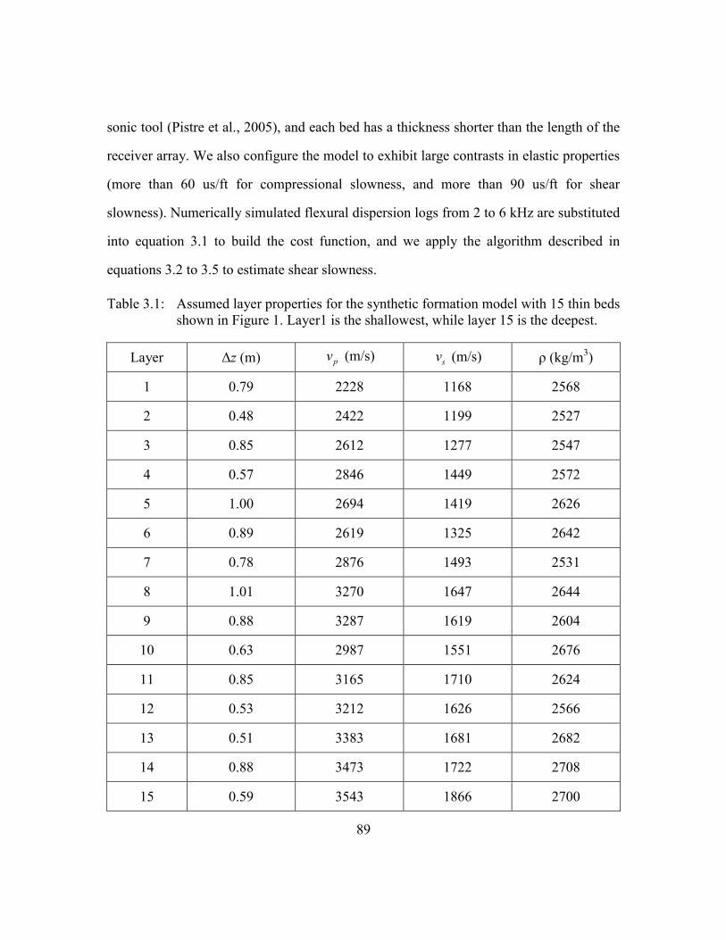
89
sonic tool (Pistre et al., 2005), and each bed has a thickness shorter than the length of the
receiver array. We also configure the model to exhibit large contrasts in elastic properties
(more than 60 us/ft for compressional slowness, and more than 90 us/ft for shear
slowness). Numerically simulated flexural dispersion logs from 2 to 6 kHz are substituted
into equation 3.1 to build the cost function, and we apply the algorithm described in
equations 3.2 to 3.5 to estimate shear slowness.
Table 3.1: Assumed layer properties for the synthetic formation model with 15 thin beds
shown in Figure 1. Layer1 is the shallowest, while layer 15 is the deepest.
Layer Δz (m) pv (m/s) sv (m/s) ρ (kg/m
3)
1 0.79 2228 1168 2568
2 0.48 2422 1199 2527
3 0.85 2612 1277 2547
4 0.57 2846 1449 2572
5 1.00 2694 1419 2626
6 0.89 2619 1325 2642
7 0.78 2876 1493 2531
8 1.01 3270 1647 2644
9 0.88 3287 1619 2604
10 0.63 2987 1551 2676
11 0.85 3165 1710 2624
12 0.53 3212 1626 2566
13 0.51 3383 1681 2682
14 0.88 3473 1722 2708
15 0.59 3543 1866 2700

90
Figure 3.1: Vertical distributions of (a) shear slowness, (b) compressional slowness, and
(c) density for the synthetic model consisting of 15 thin beds.

91
In the subsequent inversion results, 5% Gaussian noise is introduced into the data
at each frequency in the form
1i id d , (3.6)
where β is chosen such that the noise has a zero mean and a 5% standard deviation with
respect to the original data. We assign a shear velocity of 2100 m/s (equivalent to145.1
us/ft) to each layer in our starting model. On the other hand, because density sensitivity is
much lower than shear sensitivity, we assign each layer a constant density of 2600 kg/m3
for all inversion runs. For the same reason, compressional velocities are not inverted
either: we assume that the compressional velocity of each layer is 1.9 times its shear
velocity.
The inversion algorithm estimates the shear slownesses by progressively
minimizing the cost function in equation 3.1. Figure 3.2(a) shows the solution for shear
slowness, which agrees well with the true model. Although compressional slowness and
density of the layers do not agree with the model values, because the flexural mode has
very low sensitivities on the two properties, no significant biases are introduced into the
estimations. Figure 3.2(b) compares inverted slowness logs from 2 to 6 kHz to the
corresponding logs obtained using numerical simulation. The modeled logs confirm that
the algorithms have reproduced the simulated logs at convergence. We also monitor the
misfit between the modeled and the simulated logs, which drops to a constant low level
within 5 iterations, verifying that the inversion algorithm has a high convergence rate.
Table 3.2 quantitatively compares the estimated shear slownesses to the model,
accompanied by the analysis of uncertainty. Maximum relative error in the estimations
equals 1.5%. Error bars included in Figure 3.2(a) represent one standard deviation,
meaning that the model estimate will fall within this range 68% of the time. The
uncertainty in estimated shear slowness is higher for thin beds with pronounced shoulder-

92
bed effects (from 2 to 4 m), where the maximum relative uncertainty equals 2.6%. In
Figure 3.2(a), the maximum difference between the estimations and the log equals 10
us/ft, which implies that conventional well-log analysis can give rise to 6% relative
errors. The inversion method improves the log resolution from 1.83 m (the tool aperture)
to 0.51 m (the thickness of the thinnest bed resolved), equivalent to a 70% enhancement.
Table 3.2: Inversion results of shear slowness for the synthetic formation with 15 thin
beds (Figure 3.1). Layer1 is the shallowest, while layer 15 is the deepest.
Layer Initial (us/ft) Inverted (us/ft) True (us/ft) Error (%)
1 145.1 258.9±1.1% 260.9 –0.8
2 145.1 256.9±1.3% 254.2 1.1
3 145.1 235.3±2.6% 238.8 –1.5
4 145.1 210.3±1.5% 210.4 –0.1
5 145.1 212.8±1.4% 214.8 –0.9
6 145.1 229.5±1.3% 230.0 –0.2
7 145.1 201.5±0.8% 204.1 –1.3
8 145.1 185.6±0.6% 185.0 0.3
9 145.1 186.3±0.9% 188.3 –0.9
10 145.1 198.0±0.5% 196.6 0.7
11 145.1 176.1±0.8% 178.2 –1.2
12 145.1 189.8±2.2% 187.4 1.2
13 145.1 181.4±1.7% 181.3 0.1
14 145.1 177.2±2.6% 177.0 0.1
15 145.1 162.0±1.0% 163.4 –0.8

93
Figure 3.2: Inversion results for the synthetic formation model consisting of 15 thin
beds (Figure 1). (a) Estimated vertical distribution of shear slowness: the
continuous curve is the shear slowness log from numerical simulation, the
thick blocky line plotted in gray is the true model, and the dashed blocky
line with error bars designates the estimation. The error bars represent
uncertainties in the estimations obtained by including 5% Gaussian noise in
the simulated logs. (b) Flexural mode slowness logs: the solid logs are
obtained using numerical simulations, and the circles are estimated using
our method.
94
Inversion results for the synthetic case encourage us to apply the algorithm to a
field example of a siliciclastic sequence. Figure 3.3 shows the measured logs: gamma ray,
calipers, compressional and shear slownesses, micro resistivity images, and density. The
caliper logs confirm that the sonic measurements are not contaminated by borehole-size
related deleterious effects. The well is logged with the same wireline tool assumed in the
previous example. Because the sonic logs have a lower resolution than other
measurements, we jointly define 15 thin beds that value the features on resistivity,
gamma ray, and resistivity measurements (Ijasan et. al., 2014). Additionally, because the
slowness contrast between two consecutive beds is not necessarily equivalent to the
contrasts in resistivity, gamma ray, and density, we adjust the bed boundaries to ensure
that all the peaks occurring in the sonic logs are appropriately aligned with the center of a
particular bed. By analogy with the synthetic case, compressional slowness and density
are not inverted, and we adapt the log readings at centers of the beds as known inputs for
forward modeling.
Figure 3.4(a) shows the inverted shear slowness distribution accompanied by the
measured shear slowness log, and Figure 3.4(b) compares the modeled flexural
dispersion logs to the ones obtained by processing measured waveforms. The presented
error bars confirm that the estimations have low uncertainties (less than 1.6%). Figure
3.4(a) also shows that thin-bed-introduced averaging effects have been suppressed by the
inversion algorithm: the maximum difference between the estimated shear slowness and
the measured log is 8.4%.

95
Figure 3.3: Measured logs used to determine bed boundaries. From left to right, the logs
are: depth, gamma ray, caliper 1 and 2, compressional and shear slowness,
resistivity image 1 to 4, and density. Bed boundaries are plotted as
horizontal lines, and each horizontal thin bed is highlighted in green. The
top and bottom zones are not considered for inversion to avoid the
deleterious influence of borehole washouts. The image logs are displayed
using heated colormaps. The color scale ranges from 50 to 700,
corresponding to high to low resistivity.
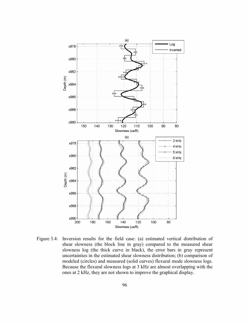
96
Figure 3.4: Inversion results for the field case: (a) estimated vertical distribution of
shear slowness (the block line in gray) compared to the measured shear
slowness log (the thick curve in black), the error bars in gray represent
uncertainties in the estimated shear slowness distribution; (b) comparison of
modeled (circles) and measured (solid curves) flexural mode slowness logs.
Because the flexural slowness logs at 3 kHz are almost overlapping with the
ones at 2 kHz, they are not shown to improve the graphical display.

97
3.3 JOINT INVERSION OF COMPRESSIONAL AND SHEAR SLOWNESSES
Flexural dispersion data enable accurate estimation of formation shear slowness,
but is limited by measurement sensitivity, whereby estimating formation compressional
slowness using the same data is challenging. In this section, we address the simultaneous
inversion of compressional and shear slownesses using P- and S- mode slowness logs.
Appendix B introduces the forward modeling method used to simulate P- and S- mode
slowness logs. Important rock mechanical parameters, e.g. Poisson’s ratio and Young’s
modulus, are also calculated from the estimated slownesses.
The same inversion algorithm previously developed for the flexural mode can be
applied to estimate compressional and shear slowness, separately. However, such a
procedure may yield inconsistent estimates in elastic properties. For most natural rocks,
the vp /vs ratio of the rock falls within the range of 2 / 2.5p sv v , where the lower
bound is compulsory for the inversion algorithm to yield positive estimates of elastic
moduli. We propose a joint inversion method that combines P- and S- mode slowness
logs to estimate elastic properties that are consistent with the vp /vs ratio constraints.
Two new moduli are defined for joint inversion as
2
S
2
p
U V ,
L V 2U,
(3.7)
Formulating the joint inversion algorithm in terms of L and U automatically ensures that
the vp /vs ratio calculated from two moduli is greater than or equal to the lower bound of
2 . The model vector that combines the moduli of all layers is given by
1 1m L , ,L , U , , UT
B B , (3.8)
while the data vector is also modified accordingly as
d d , dT
P S , (3.9)

98
where dP and dS are measured (in field cases) or numerically simulated (in synthetic
examples) P- and S- mode slowness logs, respectively, and superscript T denotes the
transpose operation. By substituting equations 6 through 9 into equations 3.2 through 3.5,
we find that the size of the Jacobian matrix grows to 4×A×B; therefore, in each iteration
the forward modeling needs to be invoked 4×A×B times, but the algorithm kernel
(Levenberg-Marquardt method) requires no change.
The joint inversion algorithm is first tested on the two synthetic verification
examples described in Table 3.3.
Table 3.3: Assumed layer properties for the synthetic formation models. Layer1 is the
shallowest, while layer 5 is the deepest in both models.
Model Layer Δz (m) pv (m/s) sv (m/s) ρ (kg/m3)
1
1 ∞ 2500 1400 2580
2 0.762 1940 1110 2540
3 0.914 2500 1400 2580
4 0.701 3420 1870 2625
5 ∞ 2500 1400 2580
2
1 ∞ 2580 1300 2580
2 0.762 1940 1110 2540
3 0.914 3100 1600 2590
4 0.732 3420 1870 2625
5 ∞ 2700 1450 2600
3
1 ∞ 2960 1600 2650
2 0.792 2680 1440 2620
3 0.853 4190 2150 2710
4 0.792 2680 1440 2620
5 ∞ 2960 1600 2650

99
In Synthetic Model 1, the thin beds 2, 3, and 4 are unevenly shouldered by layers
having different elastic properties. Layers 2 and 3 have a compressional slowness
difference of 60 us/ft and a shear slowness difference of more than 80 us/ft. Figure 3.5
shows that at convergence, the logs simulated by forward modeling agree well with the
ones obtained from numerical simulations. Quantitatively, the maximum relative errors
equal 2.2% and 3% for compressional and shear slowness, respectively. Accompanying
the logs are the initial guesses, the model values and the estimations. The joint inversion
algorithm has converged to a solution that closely approximates the actual model
properties. By comparing the estimations to the simulated logs, we infer that conventional
log interpretation without inversion can introduce errors of as much as 10% and 12% for
compressional and shear slownesses, respectively.
Synthetic Model 2 consists of three thin beds in a homogeneous background
formation. Figure 3.6 compares simulated and modeled logs, and displays inversion
results. Modeled logs upon convergence closely reproduce the numerically simulated
ones. Comparison of results shows that simulated logs are significantly influenced by the
averaging effects, making it difficult for bed boundary detection. When the tool logs from
layer 4 to layer 2, the logs provide weighted averages across the fast layer, layer 3.
Because layer 3 is remarkably faster than layers 2 and 4, the slowness peaks for layer 2
and 4 are offset by layer 3, which apparently biases the peak locations. Bed-geometry
introduced variation in the estimates will be discussed in the following example.
Synthetic Model 3 consists of three thin beds in a homogeneous background
formation. Figure 3.7 compares simulated and modeled logs, and displays the inversion
results. Modeled logs upon convergence closely reproduce the numerically simulated
ones. Comparing to the estimations, simulated logs are significantly influenced by the
averaging effects, making it difficult for bed boundary detection. When the tool logs from
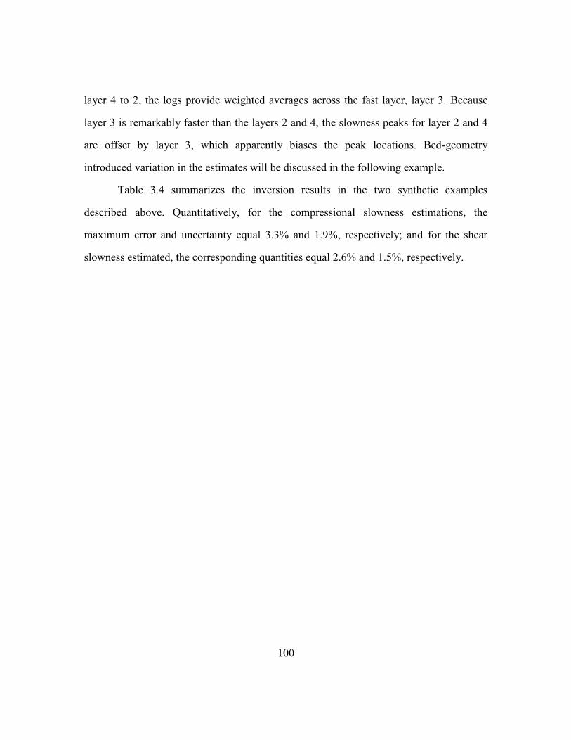
100
layer 4 to 2, the logs provide weighted averages across the fast layer, layer 3. Because
layer 3 is remarkably faster than the layers 2 and 4, the slowness peaks for layer 2 and 4
are offset by layer 3, which apparently biases the peak locations. Bed-geometry
introduced variation in the estimates will be discussed in the following example.
Table 3.4 summarizes the inversion results in the two synthetic examples
described above. Quantitatively, for the compressional slowness estimations, the
maximum error and uncertainty equal 3.3% and 1.9%, respectively; and for the shear
slowness estimated, the corresponding quantities equal 2.6% and 1.5%, respectively.

101
Figure 3.5: Inversion results for Synthetic Model 1 described in Table 3.3: estimated
vertical distributions of (a) compressional slowness and (b) shear slowness.
In each subplot, the thin curve is numerically simulated log, triangles
represent modeled log obtained at convergence, the dashed-dots represent
initial guess, the thick blocky line represent model parameters, and the
dashed blocky line with error bars represents estimated slownesses.

102
Figure 3.6: Inversion results for Synthetic Model 2 in Table 3.3: estimated vertical
distributions of (a) compressional slowness and (b) shear slowness. In each
subplot, the thin curve is the numerically simulated log, triangles represent
the modeled log obtained at convergence, the dashed-dots represent initial
guess, the thick blocky line represent model parameters, and the dashed
blocky line with error bars represent estimated slownesses.

103
Figure 3.7: Inversion results for Synthetic Model 3 in Table 3.3: estimated vertical
distributions of (a) compressional slowness and (b) shear slowness. In each
subplot, the thin curve is the numerically simulated log, triangles represent
the modeled log obtained at convergence, the dashed-dots represent initial
guess, the thick blocky line represent model parameters, and the dashed
blocky line with error bars represent estimated slownesses.

104
Table 3.4: Estimation of compressional and shear slownesses for the synthetic models in
Table 3. Layer1 is the shallowest, while layer 5 is the deepest in each model.
Model Layer Inverted
ps (us/ft)
True ps
(us/ft)
Error in
ps (%)
Inverted
ss (us/ft)
True ss
(us/ft)
Error in
ss (%)
1
1 122.6±0.4% 121.9 0.6 217.7±0.4% 217.7 0.0
2 157.0±1.1% 157.1 –0.0 279.2±0.8% 274.6 1.7
3 125.6±1.0% 121.9 3.0 221.1±0.8% 217.7 1.6
4 85.8±0.8% 89.1 –3.7 163.2±1.1% 163.0 0.1
5 122.0±0.4% 121.9 0.8 219.5±0.4% 217.7 0.8
2
1 124.9±0.7% 124.4 0.4 235.0±0.6% 234.5 0.6
2 161.4±1.6% 157.1 2.6 279.4±1.2% 274.6 1.7
3 100.3±1.5% 98.3 2.0 195.0±1.1% 190.5 2.3
4 86.3±1.9% 89.1 –3.3 162.7±1.6% 163.0 –1.7
5 112.6±0.8% 112.9 0.2 211.5±0.5% 210.2 0.2
3
1 102.8±0.8% 102.9 –0.1 190.1±0.7% 190.5 –0.2
2 117.3±1.4% 113.7 3.0 211.4±1.4% 211.7 –0.1
3 73.3±1.2% 72.7 0.7 145.6±1.5% 141.8 2.6
4 113.7±1.5% 113.7 0.1 216.3±1.5% 211.7 2.1
5 103.5±0.7% 102.9 0.5 188.2±0.7% 190.5 –1.2

105
Previously in the synthetic example shown in Figure 3.1, we estimated shear
slowness from flexural mode dispersions, we now apply the joint inversion algorithm to
the same example and estimate compressional and shear slownesses simultaneously.
Figure 3.8 shows the solutions for compressional and shear slownesses, accompanied by
the simulated P- and S- mode slowness logs, and Table 3.5 summarizes errors and
uncertainties in the estimates. The estimations agree well with the model parameters:
maximum relative errors for compressional and shear slownesses are 2.1% and 1.7%,
respectively. Furthermore, in the last column of Table 3.5, we list the vp/vs ratio of each
layer calculated from the estimated compressional and shear slownesses, which confirms
that joint inversion has yielded estimations consistent with the natural bounds.
Additionally, the algorithm features a high convergence rate: the solution is obtained
within 6 iterations.
Both inversion algorithms can estimate formation shear slowness, thus we need to
discuss the difference between the two by analyzing the results. Estimations yielded by
both algorithms show good agreement with the true values, but we notice evident
increases of uncertainties in the results obtained using the joint inversion, shown in
column 2 of Table 3.5. When flexural dispersions are used, the logs at different
frequencies are independent and function as inversion constraints, consequently the
inversion algorithm has a high tolerance for Gaussian noise. In contrast, the joint
inversion algorithm employs only compressional and shear slowness logs. Lacking of
additional constraints, these estimations are more likely to be influenced by noise.
Consequently, in Table 3.5, the maximum uncertainties for compressional and shear
slowness equal 5.5% and 6%, respectively. In addition, because the joint inversion
algorithm does not require dispersion processing, it saves more than 80% of computation
time

106
Another advantage of joint inversion is that it enables calculation of other rock
mechanical parameters, such as Poisson’s ratio and Young’s modulus. Figure 3.9 displays
the results of Poisson’s ratio and Young’s modulus derived from the slowness
estimations. The derived parameters (dashed blocky lines) agree with the model (thick
blocky lines). Uncertainties in the derived parameters are represented by the horizontal
error bars. Young’s modulus in general has a low uncertainty (5.5%), whereas the
uncertainty in Poisson’s ratio is much higher (up to 20%). Because Poisson’s ratio is
essentially a function of the vp /vs ratio, when Gaussian noise is added to the data, the
errors in both vp and vs propagate through the division operation and result in high
uncertainty in Poisson’s ratio. We also verify that other derived moduli, e.g., bulk and
shear moduli, behave similarly to Young’s modulus. Although the inversion algorithm
can be developed in terms of different rock elastic properties, i.e., velocity, slowness, or
elastic moduli, we highly recommend using the newly defined moduli, L and U, because
velocities derived from the two moduli are always self-consistent, and the inversion
algorithm formulated in terms of L and U requires no assumptions in formation density.
Inversion results presented herein are obtained under the assumption of precisely
defined bed boundaries. Next, we perturb the bed boundaries to study the influence of ill-
defined bed boundaries on the estimations. Because the sonic tool assumed in this paper
has an aperture longer than thickness of the thin beds in the synthetic formation, not all
bed boundaries can be resolved from the simulated logs. According to the simulated sonic
logs, we define five thick beds from 3.4 to 9.1 m. In Figure 3.10, we show the new
estimations compared to the ones previously obtained with the true bed boundaries.
Estimated slowness in a particular thick bed is an averaged value of the slownesses of the
original thin beds that are aligned with the thick bed. Maximum error introduced by the
boundary perturbations equals 8 us/ft (equivalent to 8.4%), which occurs at the layer

107
centered at 7 m. Bed boundaries jointly determined using high-resolution well logs, e.g.,
nuclear and resistivity image logs, can prevent errors associated with bed-geometry
uncertainty.
Table 3.5: Joint inversion results for the synthetic formation with 15 thin beds (Figure
3.1). Layer1 is the shallowest, while layer 15 is the deepest.
Layer Inverted ss
(us/ft)
True ss
(us/ft)
Error in ss
(%)
Inverted ps
(us/ft)
True ps
(us/ft)
Error in
ps (%)
Inverted
p sv v
1 259.4±3.3% 260.9 –0.6 135.6±2.0% 136.8 –0.9 1.91
2 251.8±4.3% 254.2 –1.0 125.8±5.1% 125.9 –0.1 2.04
3 237.4±2.6% 238.8 –0.6 116.9±2.5% 116.7 0.2 2.01
4 211.6±4.0% 210.4 0.6 105.9±3.9% 107.1 –1.1 1.99
5 216.4±1.6% 214.8 0.8 113.7±1.9% 113.1 0.5 1.87
6 228.3±1.4% 230.0 –0.7 115.4±1.5% 116.4 –0.8 1.99
7 204.4±1.6% 204.1 0.1 105.6±1.7% 106.0 –0.3 1.91
8 187.8±1.4% 185.0 1.4 93.9±1.3% 93.1 0.7 1.98
9 188.0±1.5% 188.3 –0.2 92.5±1.9% 92.7 –0.3 2.02
10 197.6±2.8% 196.6 0.5 102.5±2.7% 102.0 0.4 1.93
11 178.3±3.0% 178.2 0.1 96.7±2.9% 96.3 0.4 1.82
12 188.7±3.9% 187.4 0.7 92.9±5.3% 94.9 –2.1 2.04
13 178.3±6.0% 181.3 –1.7 91.7±5.5% 90.1 1.8 1.98
14 179.7±2.7% 177.0 1.5 87.0±2.3% 87.8 –0.9 2.04
15 165.2±2.3% 163.4 1.1 86.9±2.6% 86.0 1.1 1.86

108
Figure 3.8: Joint inversion results in the synthetic formation consisting of 15 thin beds
(Figure 3.1). Estimated vertical distribution of (a) compressional slowness,
and (b) shear slowness: the thin curves are the simulated logs, the thick
blocky lines represent model parameters, and the dashed blocky lines with
error bars represent the estimations.
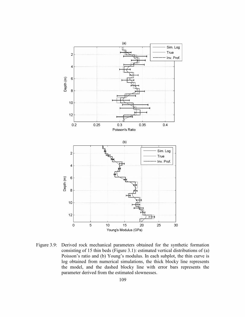
109
Figure 3.9: Derived rock mechanical parameters obtained for the synthetic formation
consisting of 15 thin beds (Figure 3.1): estimated vertical distributions of (a)
Poisson’s ratio and (b) Young’s modulus. In each subplot, the thin curve is
log obtained from numerical simulations, the thick blocky line represents
the model, and the dashed blocky line with error bars represents the
parameter derived from the estimated slownesses.

110
Figure 3.10: Estimated vertical distributions of compressional slowness (a) with precisely
defined bed boundaries and (b) with perturbed bed boundaries; and
estimated vertical distributions of compressional slowness (c) with precisely
defined bed boundaries and (d) with perturbed bed boundaries. In each
subplot, the thin curve is simulated log, the thick blocky line represents the
model, the dashed blocky line with error bars represents the estimations, and
the horizontal dotted lines are bed boundaries.

111
Summarizing the results shown in Figure 3.10, we crossplot bed thickness with
uncertainty and obtain a nearly linear relationship, as Figure 3.11 displays. Figure 3.11
also confirms that the resolution limit of the join inversion method equals approximately
0.5 m. When beds are thinner than the limit, there are too few data points to constrain the
inversion; numerical noise is likely to dominate, thus undermining the accuracy of the
estimations. For rock formations having fine-laminations, one can model the laminations
as a thick medium with vertical transverse isotropy (Backus, 1962) and then apply our
method to estimate bulk elastic properties.
The above analysis shows that our inversion method has a resolution limit of 0.5
m. Multi-shot (waveform-matching) processing techniques (Hsu and Chang, 1987; Zhang
et al., 2000) use redundant information contained in overlapping receiver subarrays to
provide improvements in vertical resolution, up to 0.4572 m (1.5 ft). However, a common
drawback of using such techniques is that for a small subarray that includes few traces,
semblance of stacked waveforms becomes susceptible to noise, which increases the
slowness estimation error. Our inversion method uses waveforms recorded at all receivers
and does not sacrifice noise-tolerance of the measurements. Our method can be used in
conjunction with multi-shot semblance techniques to provide stable high-resolution
interpretations of sonic logs.

112
Figure 3.11: Crossplot of bed thickness and uncertainty summarized from the results
shown in Figure 3.10.
Lastly, we apply the joint inversion algorithm to the same clastic sequence shown
in Figure 3.3. Figures 3.12 and 3.13 show the estimated slownesses and the derived rock
mechanical parameters, respectively. Difference between the estimations and the
measured logs indicates that conventional interpretation can result in 5% and 6% of
errors in compressional and shear slownesses, respectively. Quantitative summary of the
estimated slownesses are provided in Table 3.6. The vp /vs ratios given in the last column
confirm that the elastic properties obtained using the joint inversion algorithm are
consistent with the rock physical constraints. We also point out that the joint inversion
algorithm is consistent with the inversion algorithm introduced in last section: the
maximum difference between the shear slowness estimations given in Table 3.2 and
Table 3.6 is as low as 3.9%.

113
Table 3.6: Joint inversion results for the field case (Figure 3.3). Layer1 is the shallowest,
while layer 15 is the deepest.
Layer Δz (m) ss (us/ft) ps (us/ft) p sv v
1 0.91 121.5±2.1% 72.9±1.9% 1.67
2 0.97 110.5±2.0% 64.7±1.5% 1.71
3 1.00 116.2±2.7% 71.0±2.1% 1.64
4 0.93 101.7±2.1% 63.0±2.9% 1.62
5 0.69 104.4±1.8% 64.9±2.4% 1.61
6 0.78 118.0±1.7% 70.0±2.7% 1.69
7 0.67 118.9±1.6% 72.1±2.4% 1.65
8 0.95 107.9±1.6% 67.3±2.2% 1.60
9 0.87 103.3±3.2% 63.8±2.2% 1.62
10 0.89 127.3±2.4% 75.5±1.8% 1.69
11 0.81 111.6±2.4% 68.0±1.1% 1.64
12 0.89 100.9±3.2% 63.3±2.2% 1.59
13 0.80 109.2±2.1% 69.2±2.3% 1.58
14 0.85 108.2±1.4% 66.1±2.4% 1.64
15 0.94 122.0±1.5% 72.6±3.0% 1.68
114
Figure 3.12: Joint inversion results obtained using compressional and shear slowness logs
in the field case (Figure 3.3): (a) compressional slowness and (b) shear
slowness. The thick curves are measured logs, circles represent modeled
logs obtained at convergence, and the blocky lines with error bars are the
slowness estimates.

115
Figure 3.13: Derived parameters in the field case (Figure 3.3): (a) Poisson’s ratio and (b)
Young’s modulus. The thick curves are logs derived from field
measurements, circles represent logs derived from the inverted slowness
logs, and the blocky lines with error bars are estimations derived from the
estimated slownesses shown in Figure 3.12.

116
Figure 3.14 shows the logs from another interval. According to the logs, 19 thin
beds are jointly defined, as the horizontal lines indicate. We apply the joint inversion
algorithm to estimate compressional and shear slownesses of each layer using the P- and
S- mode logs shown in the third track.
Figure 3.14: Measured logs for determining the bed boundaries. From left to right, the
logs are: depth, gamma ray, compressional and shear slowness, resistivity
image 1 to 4, and density. Bed boundaries are plotted as horizontal lines,
and each zone is highlighted in gray.
Compressional and shear slowness estimations obtained at the convergence are
plotted in Figure 3.15, and Figure 3.16 shows Poisson’s ratio and Young’s modulus,
accompanied by their uncertainties. Measured and simulated slowness logs are also
shown and compared. Detailed inversion results are summarized in Table 3.8. The
inversion method also provides evident resolution enhancements: differences between the

117
estimations and the logs are up to 8.2% and 5.6% for compressional and shear
slownesses, respectively.
Additionally, in Figure 3.17, we compare modeled slowness logs at convergence
to the measured ones. Apparently, the modeled logs are smoother than measured ones,
especially for modeled P-mode slowness log from x961 to x962 m. Subject to
environmental noise from signal acquisition, measured logs may be spiky. The forward
and inverse method we developed is based on weighted spatial average of the formation
elastic properties, and hence provides smooth synthetic logs. The method can tolerate
noise-induced spikes in the logs.
Lastly, we discuss joint detection of bed boundaries. Previously in the synthetic
example (Figure 3.1) we perturbed the boundaries and studied bed-geometry related
uncertainty in the estimates; in Figure 3.18, we present measured P-mode log, estimated
P-mode slowness, and the density log. Three bed boundaries from x971.7 m to x973.5 m
are also shown as dotted horizontal lines. Comparing the blocky line to measured
slowness log, we notice that, due to thin-bed effect, the log shows only one peak for two
beds. On the contrary, because density measurement has a higher vertical resolution, two
peaks in accordance with the two thin beds can be clearly identified on the density log.
Joint bed-boundary determination using high-resolution logs is required to ensure
accuracy of sonic log interpretation.

118
Figure 3.15: Joint inversion results obtained using compressional and shear slowness logs
in the field case (Figure 3.14): (a) compressional slowness and (b) shear
slowness. The thick curves are measured logs, circles represent modeled
logs obtained at convergence, and the blocky lines with error bars are the
slowness estimates.

119
Figure 3.16: Derived parameters in the field case (Figure 3.14): (a) Poisson’s ratio and
(b) Young’s modulus. The thick curves are logs derived from field
measurements, circles represent logs derived from the inverted slowness
logs, and the blocky lines with error bars are estimations derived from the
estimated slowness profiles shown in Figure 3.15.

120
Table 3.8: Joint inversion results for the field data shown in Figure 3.14. Layer1 is the
shallowest, while layer 19 is the deepest.
Layer Δz (m) ss (us/ft) ps (us/ft) p sv v
1 1.06 138.7±0.9% 80.5±1.0% 1.72
2 0.83 134.2±1.5% 78.1±1.3% 1.72
3 0.79 139.8±1.5% 81.6±1.7% 1.71
4 0.77 114.9±2.0% 73.8±2.0% 1.56
5 0.90 126.5±1.5% 70.6±1.6% 1.79
6 0.88 132.6±1.3% 80.5±1.4% 1.65
7 0.88 118.3±1.3% 66.3±1.5% 1.78
8 0.88 115.0±1.5% 65.2±1.5% 1.76
9 0.96 136.9±1.3% 81.3±1.2% 1.68
10 0.78 123.8±1.6% 74.1±1.7% 1.67
11 0.75 111.7±1.7% 65.7±1.9% 1.70
12 1.04 113.3±1.0% 63.4±1.2% 1.79
13 1.06 127.4±0.9% 75.4±1.2% 1.69
14 0.89 120.8±1.3% 69.8±1.4% 1.73
15 0.84 126.5±1.3% 77.7±1.3% 1.63
16 1.02 101.1±1.3% 55.4±1.4% 1.82
17 0.71 118.9±1.6% 70.5±1.8% 1.69
18 1.08 117.0±1.0% 69.5±1.1% 1.68
19 0.69 120.6±1.5% 68.0±1.6% 1.77

121
Figure 3.17: Simulated slowness logs at convergence comparing to the measured ones in
the field case (Figure 3.14) for (a) P- and (b) S- modes.

122
Figure 3.18: (a) Measured P-mode slowness log (thick curve) and the estimated vertical
distribution of compressional slowness (blocky line). (b) Density log. Dotted
horizontal lines on each plot represent bed boundaries.
3.4 CONCLUSIONS
We developed an inversion-based interpretation method to estimate layer-by-layer
elastic properties of rock formations from borehole sonic measurements. The method
utilizes sonic spatial sensitivity functions for fast forward modeling, and estimates in-situ
elastic properties of rock formations by reproducing the measured dispersion and
slowness logs with numerical simulations.
Two algorithms were developed based on the same inversion workflow. The first
algorithm uses flexural mode dispersion logs at multiple discrete frequencies to estimate
formation shear slowness; it was applied to a noisy synthetic case in which a vertical well
penetrated multiple horizontal thin beds. Shear slownesses of thin beds were estimated to
within a few percent of the true values, accompanied by low uncertainties (2.6%). The

123
algorithm also enhanced the vertical resolution of the measurement to approximately 0.5
m. Application of the inversion algorithm to noisy field data confirmed that the method
decreases shoulder-bed effects and provides reliable estimates of formation shear
slowness.
The second algorithm addressed the problem of simultaneous inversion of
compressional and shear slownesses. By combining P- and S- mode slowness logs, we
formulated the joint inversion algorithm in terms of elastic moduli to ensure that
estimated elastic properties were self-consistent. Results obtained with the same synthetic
and field data confirmed the efficiency and reliability of the algorithm to improve the
vertical resolution of the original sonic logs. Compared to the first inversion algorithm,
the joint inversion algorithm saves more than 80% of computation time at a price of
slightly increased uncertainty (from 2.6% to 6%). After estimating both compressional
and shear slowness estimations, we estimated and appraised other related rock
mechanical parameters. We summarize that Young’s modulus and other moduli
calculated from the slownesses have low uncertainties, whereas the Poisson’s ratio has
moderate to high uncertainty.
Lastly, both inversion algorithms have high stability and convergence rates;
convergence is usually reached within only a few iterations. The research presented
suggests that inversion-based petrophysical interpretations can be developed to integrate
modern sonic logs with other well logs for improved formation evaluation.

124
Chapter 4: Fast forward modeling of borehole sonic measurements in
high-angle and horizontal wells
In vertical sections of a well, sonic waves propagate perpendicular to the bed
boundaries, and hence the wave field is homogeneous in borehole azimuthal direction.
However, in high-angle wells with dipping layers, rock formations in the proximity of the
wellbore exhibit three-dimensional variations. Mode interference and conversion occur at
every depth, especially when a layer interface intersects the receiver array. As a result,
the dispersion of flexural mode obtained in high-angle and horizontal wells often show
low-frequency distortions, which make it difficult to identify the low-frequency
asymptote corresponding to formation shear slowness. We extend spatial sensitivity
functions to 3D to model high-frequency dispersion, circumventing the distortion effect
at the low frequencies.
In addition to the dispersive modes, non-dispersive compressional (P-) and shear
(S-) modes are routinely measured in modern borehole acoustic logging. Slownesses
(inverse of velocity) of the P- and S-mode provide information on compressional and
shear slownesses of the rock formation surrounding the wellbore, respectively. When a
high-angle well penetrates horizontal thin layers, the layers function as waveguides for
sonic waves to propagate. The layer-trapped waves and the borehole-guided ones
interfere with each other and result in amplitude variation and phase discontinuity in the
waveforms registered at the receivers. Consequently, the waveforms measured across the
receiver array often show low semblance, which renders the conventional waveform
semblance-based processing techniques inadequate to provide reliable estimation of
formation slowness. In this chapter, instead of calculating waveform semblance, we refer
to compressional first arrivals to describe the propagation of P-mode in HA/HZ wells,

125
and we derive P-arrival slowness from the first arrival times in measured waveforms.
Because first arrival at a particular receiver is induced by the earliest P-wave that arrives
at the receiver, P-arrival slowness log calculated from the first arrival times is much less
affected by mode interference than the log obtained using semblance-based processing
techniques.
A number of numerical tests in high-angle wells are performed to show that the
compressional first arrivals are mainly induced by the converted P-waves through
deviated layers. Accordingly, we introduce a one-dimensional layered model that is
capable of modeling P-mode first arrivals in HA/HZ wells across thinly bedded
formations. In a number of synthetic examples with wireline sonic logging in HA/HZ
wells, the P-arrival slowness logs predicted using our new model agree well with those
obtained using three-dimensional finite-difference simulations. Additionally, because the
new method simplifies the geometrical condition from 3D to 1D, it saves 99% of CPU
time comparing to the numerical simulations.
4.1 INTRODUCTION
In wireline sonic logging, waveforms sensed by the array receivers are processed
to quantify frequency-slowness dispersions, from which one can estimate mechanical and
petrophysical properties of the rock formations. For example, low-frequency asymptote
of the flexural mode dispersion is commonly used to estimate formation shear wave
velocity. When an HA/HZ well penetrates horizontal thin beds, elastic property of the
formation exhibits three-dimensional variations. As a result of complex geometrical
conditions, an acoustic transducer often simultaneously excites wave modes of different
orders. Interference between the modes significantly influences dispersion analysis, and
one often observes the distortion effect in flexural mode dispersion curve at the low

126
frequencies (Mallan et. al., 2013), inhibiting identification of its low-frequency
asymptote. To assist sonic log interpretation in HA/HZ wells, we develop a fast forward
modeling algorithm based on 3D semi-analytical sensitivity functions to circumvent the
distortion effect, and provide accurate prediction of sonic dispersion measurements at
high frequencies.
On the other hand, the compressional mode (in all types of formations) and shear
mode (in fast formations) are excited and measured by the tool’s monopole transmitter-
receiver system (Cheng and Toksöz, 1981). Measured monopole waveforms are routinely
processed using semblance-based method in the time domain to estimate slonwesses of
the rock formation. The estimated slownesses have multiple applications in petrophysical
formation evaluation. Because hydrocarbons in a conventional reservoir are stored in the
pore space of porous media, reservoir porosity assessment is thus one of the main tasks of
reserve estimation. Compressional and shear slowness data calculated from well-logs
have been used for more than half a century to quantify sonic porosity (Bassiounimore,
1994). For rock physical analysis, sonic porosity logs derived from P-mode measurement
can be used to provide an estimation of Voigt upper bound in compressional slowness
(Mavko et al., 1998). Apart from reserve estimation, formation mechanic properties, e.g.
Young’s modulus and Poisson’s ratio, are crucial to predict long-term deformation
behavior of the rocks. Compressional and shear slownesses estimated from borehole
sonic measurements are required to assess in-situ formation mechanic properties
(Montmayeur and Graves, 1985; Walls, 1987). In addition, compressional and shear
velocity data adapted from sonic logs are widely used in seismic applications. For
example, the velocity profiles derived from sonic logging provide constraints on the
velocity models of the earth, which are used to transform seismic time sections into depth
sections (Coates et al., 2000).

127
When a vertical well penetrates a rock formation consists of multiple horizontal
layers, propagation direction of the P- and S-waves is perpendicular to the layers. At a
particular depth, the wave fields inside and out of the wellbore are homogeneous in the
azimuthal direction, and the measured P- and S- head waves provide averaged
compressional and shear slownesses of the horizontal layers, respectively. When the tool
logs across thin beds in an HA/HZ well, in addition to the wellbore, the deviated layers
are also able to trap wave energy, i.e. the waves can travel along the layers. When the
wellbore-guided waves and the layer-trapped ones concurrently arrive at the same
receiver, different wave components begin to interfere, and one observes amplitude
fluctuation and phase discontinuity in the waveforms registered at the receivers.
Consequently, waveforms at difference traces exhibit low semblance. We document a
few synthetic examples simulated in HA/HZ wells to show that the conventional
waveform semblance-based processing technique, i.e. the Slowness-Time Coherence
(STC) method, can hardly provide reliable slowness estimations: P-mode slowness log
obtained from STC processing shows strong dependence on length of processing window
in the time domain. Due to the difficulty in STC processing, we introduce an apparent P-
mode slowness derived from first arrivals in the waveforms. The first arrival in a
particular waveform is introduced by the P-wave component that takes the fastest travel
path from the transmitter to the receiver, and thus interferes less with other late arrivals.
One can estimate first arrival time by determining the fastest travel path from the
transmitter to the receiver.
We employ the ray-tracing method to search for the fastest P-wave travel path
through the dipping layers in synthetic examples across a highly-deviated bed boundary.
Fundamentally, the ray-tracing method is invoked to calculate the path of waves (ray
path) through a system with regions of varying velocities. In seismology, ray-tracing aids

128
in tomographic reconstruction of the Earth interior layers (Cerveny, 2001; Hauser et al.,
2008). In borehole acoustic logging endeavor, Lin et al. (2006) showed that the
compressional ray path can be traced in a moderately inclined layered formation. Our
study shows that the method is also applicable to determine the ray paths in HA/HZ wells
provided that the rock formation in the proximity of the receiver array is homogeneous.
P-arrival slowness can be accurately predicted from the apparent compressional phase
slownesses at all the receivers.
However, when the formation in the proximity of the receivers exhibits strong
heterogeneity (e.g. a bed boundary intersects the receiver array), the ray-tracing method
is no longer applicable. Wave theory is required to describe phase changes and mode
interference induced by such strong elastic property heterogeneity, i.e. only three-
dimensional numerical methods are able to simulate sonic logging measurements. We
seek simplifications to the formation model to reduce the amount of simulation time.
Theoretically, P-arrivals in an HA/HZ well are jointly influenced by the converted P-
waves through the formation layers and the guided P-waves in the wellbore. Based on the
ray-tracing study, we hypothesize that the converted P-waves provide dominant
contributions to the P-arrivals. To test the hypothesis, we perform numerical simulations
in an effective multi-layered formation model without the borehole and the logging tool.
Essentially, removal of the borehole and the tool eliminates the wellbore-guided P-waves
such that our tests focus only on the converted ones. P-arrival slowness logs derived
using the new model show good agreement to the ones obtained in the original model
(which includes both the borehole and the tool) using numerical simulations, which also
validates our hypothesis. We further infer that the simplified model can be used to derive
P-arrival slowness logs in HA/HZ wells. Because the rock formations in the new model
exhibit elastic property variation only in the direction perpendicular to the bed

129
boundaries, it simplifies the problem from 3D into 1D. Therefore, we apply discrete
wavenumber integration along the real axis (Rosenbaum, 1974; Tsang and Rader, 1979;
Cheng and Toksöz, 1981) on the simplified model to synthesize the waveforms measured
by an obliquely aligned transmitter-receiver system, from which we estimate P-arrival
slowness.
In a few synthetic examples when HA/HZ wells penetrate multiple horizontal thin
beds, we apply the modeling algorithm to predict P-arrival slowness logs. The modeled
logs are compared to the ones obtained in the original models using three-dimensional
finite-difference time-domain (FDTD) simulations. Quantitative comparisons verify that
the algorithm is accurate and efficient in modeling P-arrival slowness measurement in
HA/HZ wells.
4.2 MODELING GUIDED-MODE DISPERSIONS IN HA/HZ WELLS
Using 3D FDTD simulations, Mallan et. al. (2013) showed that dipping shoulders
in high-angle wells introduce strong distortions in monopole Stoneley and dipole flexural
dispersions. The distortions at low frequencies in flexural dispersion make it formidable
to estimate formation shear velocity. We simulate waveforms acquired in an 84-degree
deviated well penetrating three transverse isotropic (TI) thin beds. Table 4.1 provides the
formation properties: mass density, vertical velocities, Thomsen’s parameters, and
vertical thickness. The tool is modeled as a heavy mud column, with its properties given
in Table 4.2. We also assume a 22.2-cm (8¾-inch) borehole for all numerical simulations
in the chapter, with pure water filling the gap between the tool and the borehole wall.
Simulated waveforms are processed to obtain the dispersion curve shown in Figure 4.1.
The curve shows evident distortions below 3.5 kHz. However, at 4 kHz and above, we

130
observe good stability that enables us to apply the spatial sensitivity functions for forward
modeling.
Table 4.1: Elastic properties of the formation layers. BG represents background
formation, L1 to L3 denote the layers. L1 and L3 are the deepest and the
shallowest, respectively.
Layer BG L1 L2 L3
ρ (kg/m3) 2600 2650 2620 2580
pvv (m/s) 4700 5501 4585 3599
svv (m/s) 2137 2408 2089 1827
ε 0 0.14 0.1 0.15
δ 0 0.11 0.08 0.06
γ 0 0.12 0.12 0.1
Δz (m) ∞ 0.4572 0.5334 0.6096
Table 4.2: Elastic and geometrical properties of the wireline logging tool.
pv (m/s) 1800
sv (m/s) 0
ρ (kg/m3) 3110.5
Number of receivers 25
Inter-receiver spacing (m) 0.0762
Frist receiver offset (m) 3.2766
Outer diameter (m) 0.046

131
Figure 4.1: Flexural dispersion results: the map and the solid curve are obtained by
processing simulated waveforms, and the triangles are estimated using
sensitivity functions. Horizontal dashed lines represent directional shear
velocities of the layers.
Because formation properties in HA/HZ wells exhibits three-dimensional
variations, we extend the sensitivity functions developed in chapter 2 to 3D (axial-radial-
azimuthal). In azimuthal direction, the measurement sensitivity is represented using
source excitation functions, i.e. unity for monopole and |cos θ| for dipole, and we
calculate 3D sensitivity function as a product of axial, radial, and azimuthal sensitivity
function, as
, , , ,, , , , , , , , ,a r z r a r r a r a z rG r z M f G r M f G M f G z M f , (4.1)
where symbol denotes tensor product. Figure 4.2 displays the sensitivity functions
calculated using equation 4.1.

132
Figure 4.2: Semi-analytical axial-radial-azimuthal sensitivity functions for (a) monopole
Stoneley mode, and (b) dipole flexural mode.

133
Using the sensitivity functions, the dispersions can be modeled according to
,
, ,
, ,, , , ,
r
r a r z r
M r z r
M r zs f s f G r z M f r r z
M
, (4.2)
where sr denotes mode slowness in the reference homogeneous formation, M
r represents
elastic property of the reference formation, and ∆M represents the perturbation of a
particular property. We model flexural and Stoneley mode dispersions when an
undulating wellbore penetrates the same rock formation given in Table 4.1. Figure 4.3
shows the well trajectory, which is split into eight intervals according to local deviation
angles, and geometrical parameters of the well are documented in Table 4.3. The tool is
up-logging in the well from intervals 8 to 1. For convenience, we set measured depth
(MD) to be zero when the measurement point is at the left end of section 1 (the leftmost
dot on the trajectory). In order to locate the measurement point with respect to the beds,
in last column of Table 4.3, true vertical depth (TVD) is also provided, which is defined
as the vertical distance from the bottom of layer L1 to the measurement point. Because
the layers are anisotropic, they are modeled using equivalent isotropic parameters. For
dipole flexural mode, we use directional quasi-P and quasi-SV velocities (Fedorov, 1968;
Musgrave, 1970; Aki and Richards, 2002) as model parameters, and the velocity
calculated using equation 4.3 provides the equivalent shear velocity for modeling
Stoneley mode dispersion (Chi and Tang, 2003),
14 12
332 2 244 66 2
sin θ1sin θ cos θ
4 1 2 sin θ /ST
cv c c
F
(4.3)
where ε and δ are Thomsen parameters, ρ is mass density, and 33 441F c c . The phase
angle, θ, is the angle between the wellbore and the symmetric axis of the TI layers. Table

134
4.4 gives the velocities of the equivalent isotropic layers calculated for all dip angles
shown in Figure 4.3.
Figure 4.1 shows modeled flexural dispersion (triangles) comparing to the
dispersion curve obtained from numerical simulation, and Figure 4.4 shows the same
comparison for Stoneley mode. Modeled logs agree well to the ones from simulations at
the frequencies selected. In Figures 4.5(a) and 4.5(b), we show comparison of flexural
and Stoneley dispersion logs, respectively. Equivalent shear slowness profiles of the
formation layers are also provided to aid analysis. Since Stoneley mode is less dispersive
than flexural mode, we only plot the Stoneley dispersion at 1 kHz. For both modes,
modeled logs show good agreement to the simulated ones. Quantitatively, the maximum
relative errors in the logs for the flexural and Stoneley mode are 2% and 1%,
respectively. In addition, we notice apparent discrepancies between modeled logs and
equivalent isotropic shear slowness profiles. Because the modeled logs represent high-
frequency dispersions, inversion-based methods are required to estimate true formation
properties.

135
Figure 4.3: Trajectory of the well penetrating three TI layers.

136
Table 4.3: Geometrical parameters of the well shown in Figure 4.3.
Interval Dip MD (m) TVD (m)
1 82, down 0:1:4 2.088:-0.1392:1.5312
2 84, down 6:2:10 1.516:-0.209:1.098
3 86, down 12:2:18 1.046:-0.1395:0.6275
4 88, down 22:4:30 0.558:-0.1396:0.2788
5 88, up 33:2:41 0.204:0.0698:0.553
6 86, up 43:2:49 0.554:0.1395:0.9725
7 84, up 50:1:55 1.04:0.1045:1.5625
8 82, up 57:2:61 1.565:0.1392:2.1218

137
Table 4.4: Equivalent isotropic parameters for the model shown in Figure 4.3.
Dip Layer qSV (m/s) qP (m/s) ,s STv (m/s)
82
L1 2413.3 6208.4 2457.4
L2 2092.1 5013.2 2155.8
L3 1835.7 4090.4 1884.6
84
L1 2411 6215.1 2455.7
L2 2090.7 5017.3 2154.1
L3 1831.9 4096.1 1883.9
86
L1 2409.4 6219.8 2454.4
L2 2089.8 5020.3 2152.9
L3 1829.2 4100.2 1883.3
88
L1 2408.3 6222.7 2453.7
L2 2089.2 5022 2152.2
L3 1827.6 4102.7 1883

138
Figure 4.4: Stoneley dispersion results: the map and the solid curve are obtained by
processing simulated waveforms, and the triangles are estimated using
sensitivity functions.

139
Figure 4.5: Comparison of (a) flexural and (b) Stoneley mode slowness logs calculated
using the sensitivity method (circles) to the ones obtained using numerical
simulations (solid). The blue blocky curve represents equivalent shear
slowness profile.

140
4.3 STC PROCESSING IN HA/HZ WELLS
Time-domain waveform coherence stacking method is commonly used for
estimation of P-mode slowness. The processing technique employs a time-slowness grid
for stacking the waveforms measured across the receiver array. Coherence of the stacked
data is calculated and compared, to locate wave arrival time and propagation slowness.
Slowness obtained at a coherence maximum may represent compressional or shear
slowness of the formation, depending on the corresponding arrival time. Kimball and
Marzetta (1986) defines the coherence as
2
1
2
1
1
,
1
w
w
T T N
m
mT
T T N
m
mT
X t s m d dt
s T
N X t s m d dt
(4.4)
where Xm represents the time-domain waveform at the m-th receiver, N is the total
number of receivers, and d is the receiver spacing. The time variable T designates the
center position of a time window with a length Tw. The variable s is a slowness value that
defines the shift of the time window between two consecutive receivers. T, Tw, and s
jointly define which portion of the waveforms will be stacked for coherence calculation.
Equation 4.4 can be used to compute a two-dimensional time-slowness semblance surface
(called a correlogram) by stepping the time window through the waveforms acquired at
the entire array. Compressional or shear slowness of the formation can be obtained at a
local maximum on the correlogram.
Essentially, the STC method back-propagates the waveform at each receiver to
the first receiver position for stacking and calculation of coherence. The underlying
assumption of the method is that, for a particular mode, the back-propagated waveforms
in the time window Tw have comparable phase behavior. In vertical wells, for the non-

141
dispersive modes, i.e., P- and S-modes, the assumption is generally satisfied. Mode
conversion happens across horizontal thin beds and provides an inhomogeneous wave
field in vertical direction. But in each layer, the wave field is homogeneous in azimuthal
direction. In such case, coherence value calculated from the stacked waveform data
quantify average phase change across the receiver array, from which one is able to
calculate an average slowness of the formation layers, weighted by the axial sensitivity
function of the measurement (provided in section 2.7). In HA/HZ wells, formation
geometry becomes more complex due to intersection of the deviated layers and the
borehole. Mode conversion and interference across the dipping bed boundaries induces
inhomogeneous wave field in radial, azimuthal, and axial directions of the wellbore.
Typically, waveforms acquired in HA/HZ wells are lack of phase continuity between
different receivers. To illustrate the problem, we simulate monopole sonic logging in two
synthetic examples, as Figure 4.6 shows. In each example, the same wireline monopole
tool, centralized in the wellbore, is logging across a 75-degree dipping boundary. Table
4.5 lists detailed elastic properties of the formations above and below the boundary. The
monopole source (the square in Figure 4.6) is present below the boundary. Lower half of
the receiver array (the circles in Figure 4.6) is in the bottom formation, while the upper
half of the array is in the top formation. Interface between the two formations intersects
the borehole axis right at the middle receiver (receiver 13), which has an offset of 4.191
m above the source along the wellbore axis.

142
Figure 4.6: Synthetic models of a wireline monopole tool logging across a 75-degree
dipping boundary. (a) The monopole source is in the slower formation
below the boundary. (b) The monopole source is in the faster formation
below the boundary.
Table 4.5: Parameters of the formations shown in Figure 4.1.
Formation A B
pv (m/s) 4100 3400
sv (m/s) 2150 1700
ρ (kg/m3) 2550 2500
In the first example shown in Figure 4.6(a), the top formation has a higher mass
density and higher velocities than the bottom one. Synthetic waveforms generated using
FDTD simulations are shown in Figure 4.7. Increase in receiver offset causes a moveout
(or delay) in wave arrivals between any two consecutive receivers. Recalling the STC
method defined in equation 4.4, we notice that the time shift factor, s, is equivalent to a

143
common moveout value for the entire array, and one can estimate the P-mode slowness
from the moveout of the P-arrivals. Graphically, one can estimate P-wave velocity from
the slope of first-arrival moveout. In Figure 4.7, as the arrows indicate, we identify a
conspicuous slope change from the bottom receivers to the top ones. The slope change
happens across the middle receiver, at the intersection of the bed boundary and the
borehole axis. Estimated from the slopes, P-waves measured at the bottom receivers is
slower than the one measured at the top receivers, which agrees with the velocities given
in Table 4.5. Moreover, the waveforms at traces 10 to 15 show notable phase
discontinuity. Because the dipping boundary introduces strong elastic property
heterogeneity in the formations surrounding of the receiver array, mode conversion and
interference result in a highly inhomogeneous wave field, which is registered at the
receivers. Consequently, we observe that measured waveforms between different
receivers exhibit low semblance, especially for the ones acquired in the proximity of the
bed boundary. If applying STC analysis on the waveforms shown in Figure 4.7, we
expect the stacked data to show low coherence.
In the second example, we simulate waveforms in the model shown in Figure
4.6(b), which assumes the same geometry as the previous example but with the formation
properties reversed. The synthetic waveforms are shown in Figure 4.8. The arrow
indicates no significant slope change observed in the first arrivals. However, in the late
arrivals circled by the dashed line, we notice that moveout slopes calculated for different
wave cycles are not in parallel, which signifies mode interference above the bed
boundary. The bed boundary effect has more influence on the late arrivals than on the
early ones. If we apply STC processing and vary the length of the processing window, Tw,
different slowness values will be obtained.

144
Figure 4.7: Synthetic waveforms obtained using the model shown in Figure 4.6(a). The
arrows show the slope change from the bottom receivers to the top ones, and
the dashed line circles the portion of waveforms showing phase
discontinuity.
Figure 4.8: Synthetic waveforms obtained using the model shown in Figure 4.6(b). The
arrow shows no significant slope change from the bottom receivers to the
top ones, whereas the waveforms circled by the dashed line are influenced
by mode interference.

145
We allow the tool to log across the formations given in the two synthetic models.
Waveforms at each tool location are simulated using the FDTD method, and we apply the
STC method to calculate P-mode slowness logs. In each example, we try two processing
windows with different length to study the stability of the processing technique. The logs
are shown in measured depth, and the depth zero is defined when the measurement point
(receiver 13) coincides with the bed boundary such that a positive/negative depth
translates into measurement point located below/above the bed boundary.
Figure 4.9(a) shows the logs calculated in the first model displayed in Figure
4.6(a). The two logs are obtained using the narrow and wide processing windows
displayed in Figure 4.9(b). The narrow processing window includes only the first P-
arrival wave cycle, whereas the wide window includes an additional cycle of late arrival.
In Figure 4.9(a), regardless of the difference in processing window, the logs below 6 m
converge to the slowness of the bottom formation, and they also converge to the top
formation slowness above –2 m. However, from –1 to 1 m, when the bed boundary
intersects with the receiver array, the two logs exhibit significant discrepancies: the
slowness values predicted by the narrow window are significantly lower than the ones
given by the wide one. As the waveforms in Figure 4.7 shows, the inhomogeneous wave
field in the proximity of the deviated bed boundary includes wave components with
different phase velocities. Earlier arrival components have higher velocities than the late
arrival ones. The wide processing window includes more lower-velocity late arrivals, and
thus provides slower estimations than the narrow one.
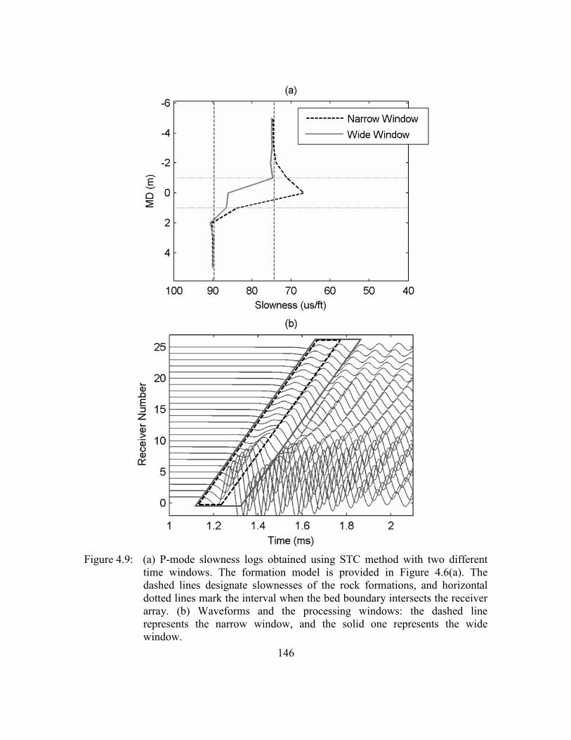
146
Figure 4.9: (a) P-mode slowness logs obtained using STC method with two different
time windows. The formation model is provided in Figure 4.6(a). The
dashed lines designate slownesses of the rock formations, and horizontal
dotted lines mark the interval when the bed boundary intersects the receiver
array. (b) Waveforms and the processing windows: the dashed line
represents the narrow window, and the solid one represents the wide
window.
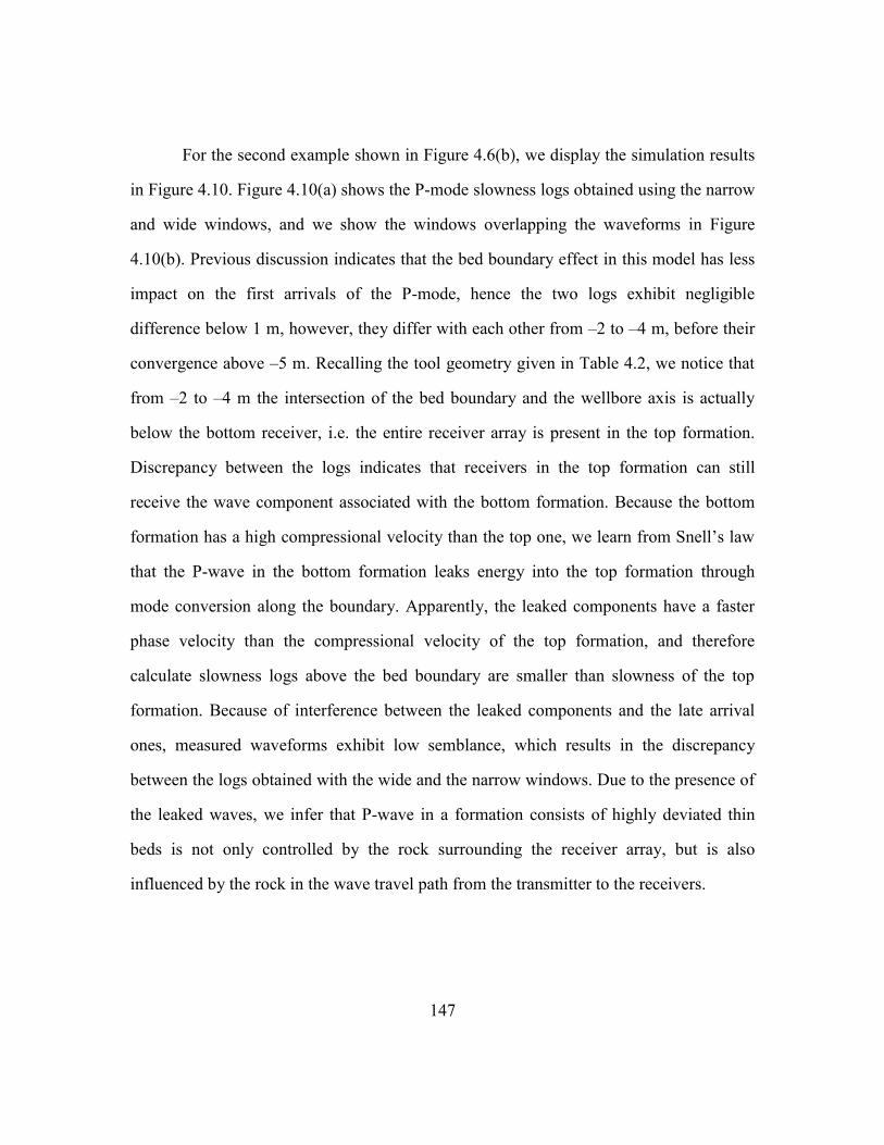
147
For the second example shown in Figure 4.6(b), we display the simulation results
in Figure 4.10. Figure 4.10(a) shows the P-mode slowness logs obtained using the narrow
and wide windows, and we show the windows overlapping the waveforms in Figure
4.10(b). Previous discussion indicates that the bed boundary effect in this model has less
impact on the first arrivals of the P-mode, hence the two logs exhibit negligible
difference below 1 m, however, they differ with each other from –2 to –4 m, before their
convergence above –5 m. Recalling the tool geometry given in Table 4.2, we notice that
from –2 to –4 m the intersection of the bed boundary and the wellbore axis is actually
below the bottom receiver, i.e. the entire receiver array is present in the top formation.
Discrepancy between the logs indicates that receivers in the top formation can still
receive the wave component associated with the bottom formation. Because the bottom
formation has a high compressional velocity than the top one, we learn from Snell’s law
that the P-wave in the bottom formation leaks energy into the top formation through
mode conversion along the boundary. Apparently, the leaked components have a faster
phase velocity than the compressional velocity of the top formation, and therefore
calculate slowness logs above the bed boundary are smaller than slowness of the top
formation. Because of interference between the leaked components and the late arrival
ones, measured waveforms exhibit low semblance, which results in the discrepancy
between the logs obtained with the wide and the narrow windows. Due to the presence of
the leaked waves, we infer that P-wave in a formation consists of highly deviated thin
beds is not only controlled by the rock surrounding the receiver array, but is also
influenced by the rock in the wave travel path from the transmitter to the receivers.
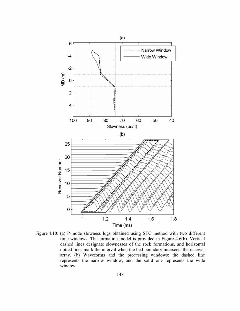
148
Figure 4.10: (a) P-mode slowness logs obtained using STC method with two different
time windows. The formation model is provided in Figure 4.6(b). Vertical
dashed lines designate slownesses of the rock formations, and horizontal
dotted lines mark the interval when the bed boundary intersects the receiver
array. (b) Waveforms and the processing windows: the dashed line
represents the narrow window, and the solid one represents the wide
window.

149
From the two synthetic examples, we conclude that, in HA/HZ wells, the STC
method strongly depends on the length of the processing window, Tw. Characterization of
P-mode propagation in HA/HZ wells requires a stable processing technique that takes
into account the influence of the dipping layers between the transmitter and the array
receivers.
4.4 P-ARRIVAL SLOWNESS IN HA/HZ WELLS
Because of complex mode interference across dipping bed boundaries, stacked
waveform data often exhibits low coherence, and the STC method can hardly provide a
reliable answer on P-mode slowness. To avoid the impact of late-arrival interference, we
refer to P-mode first arrivals to derive apparent P-arrival slowness log in HA/HZ wells.
We begin the discussion using the synthetic example shown in Figure 4.11. The wellbore
has a deviation angle of 80 degrees, and the wireline monopole tool is operating across a
dipping thin bed that has a vertical thickness of 0.6096 m. Elastic properties of the
background formation and the thin bed are provided in Table 4.5.
Figure 4.11: The synthetic model when a wireline monopole tool logs across an 80-
degree deviated thin bed, where h is the vertical thickness of the bed.

150
In Figure 4.12(a), we show synthetic waveforms simulated using the FDTD
method. The circle on each trace marks the arrival time of the P-mode. From each
consecutive receiver pair, we divide the moveout in arrival time by the inter-receiver
spacing to obtain an instant slowness value. The tool assumed has 25 receivers, and
totally 24 instant slowness values are calculated and plotted in Figure 4.12(b). Apparent
P-arrival slowness of the measurement is obtained by averaging all 24 instant slowness
values, which equals 74.5 us/ft.
Next we allow the tool to log upward across the thin bed and numerically simulate
the waveforms at a few depths, and we define measured depth to be 0 when the
measurement point coincides with the lower boundary of the dipping bed. The
waveforms are first processed using the STC method with the same two processing
windows defined in previous examples. For comparison, a P-arrival slowness log is also
derived from the instant slowness values. Subsequently, we compare the three slowness
logs in Figure 4.13.
At 2 m and below, because both the source and the receivers are in the
background formation, all three logs converge to slowness of the background. From 1 to
–1 m, each log provides a different answer of P-mode slowness. In this interval, because
the dipping bed intersects the receiver array, we observe that the STC method has strong
dependence on processing window length, and the two logs from STC processing exhibit
large discrepancies, up to 22 us/ft at depth 0. In comparison, the P-arrival slowness log
provides a smooth transition from the background formation slowness to the thin bed one.
We further notice that the transition begins two meters (in measured depth) before the
measurement point intersects the dipping bed.
The three logs generally agree with each other in the interval from –1 m to –9 m.
The logs gradually transit from the thin bed slowness to the slowness of the background,

151
which is due to the leaked waves from the fast layer into the top background formation,
similar to the phenomenon shown in Figure 4.10(a). We notice that the P-arrival slowness
log exhibits fewer fluctuations than the other two in this interval.
In sum, the P-arrival slowness log does not require waveform stacking and
semblance calculation, and thus is not influenced by phase discontinuities induced by
late-arrival interference. Consequently, in HA/HZ wells, P-arrival slowness log can be
predicted by determining the arrival time of compressional wave component at each
receiver.

152
Figure 4.12: (a) Waveforms (solid) and P-arrivals (circles). (b) Instant slowness values
obtained from every consecutive receiver pair (triangles). The dashed lines
represent compressional slownesses of the formations.

153
Figure 4.13: P-arrival slowness log comparing to logs obtained using the STC method.
4.5 ESTIMATION OF P-ARRIVAL SLOWNESS USING RAY-TRACING METHOD
In geophysical applications, ray-tracing method is useful in providing tomography
of the Earth layers with different velocities. Seismic waves can be characterized as
narrow beams (rays) propagating through the Earth layers. In borehole sonic logging, a
formation layer that can be resolved has a thickness comparable to the wavelength of
sonic signal, which satisfies the fundamental assumption of the ray-tracing method.
Approximating the P-waves as beams radiated from the source into the borehole and the
surrounding formations, we apply the ray-tracing method to track the travel path and
calculate the arrival time of each beam. P-arrival slowness is then estimated from the first
arrival times at the receivers.
We discuss the ray-tracing procedure using the model shown in Figure 4.14. The
tool logs across a dipping boundary, where the formation below is faster than the
formation above the boundary. The formation properties are given in Table 4.5. Along

154
the wellbore axis, distance from the source to the boundary, d, is fixed and equals 2 m,
whereas four different dip angles are taken into account. The dip angle, θ, is set to 65, 70,
75, and 80 degrees.
Figure 4.15(a) shows a strict ray-tracing diagram from the source to two
consecutive receivers. Because the formations have higher compressional velocities than
the borehole fluid, and the borehole radius is smaller than P-wave radial depth of
penetration, borehole-induced travel-time difference can be neglected. Consequently,
Figure 4.15(b) displays a simplified ray-tracing diagram without the borehole.
Accordingly, P-wave first arrival time at a particular receiver can be solved from
,
,
, ,
sin sin z,2 2
sin,
sin
sin cos tan d,2 2
,
A B
p A
p B
A B
A B
p A p B
p p
v
v
p p
p pt
v v
(4.5)
where t is the arrival time we are after, ,p Av and ,p Bv are the compressional velocities of
bottom and top formations, respectively, and all other variables are labeled in Figure
4.15(b). Strictly speaking, in the simplified model, the transmitter-to-receiver spacing
(TR spacing), z, and the transmitter-to-boundary axial distance, d, are slightly smaller
than the corresponding quantities in the original model (which includes the borehole).
However, numerical tests show that the differences are less than 3%. Therefore, we input
into equation 4.5 the same TR spacing and transmitter-to-boundary distance as in the
original model.

155
Figure 4.14: The synthetic model for ray-tracing analysis. The intersection of the bed
boundary and the borehole axis is between source and the bottom receiver.
Distance from the intersection to the source, d, equals 2 m.
Figure 4.15: (a) Rays across the dipping boundary from the transmitter to two
consecutive receivers. (b) Simplified ray-tracing diagram without the
borehole.

156
Equation 4.5 is solved numerically at all the receivers for the arrival times, and to
derive instant slownesses. For the selected deviation angles, instant slowness profiles
modeled using ray-tracing method are shown in Figure 4.16, accompanied by their
counterparts calculated using FDTD simulations in the original model. In all the cases,
despite numerical differences, the ray-tracing predictions agree well to the simulated
ones. As the dip angle increases, the path pA in bottom formation increases, and the path
pB in top formation decreases. Because the bottom formation is faster than the top one, it
results in a common decrease of the instant slownesses at all receivers. Figure 4.16
confirms that the ray-tracing method has correctly predicted the shift in slowness with
respect to dip angle.
At the current stage, the ray-tracing method has successfully characterized P-
mode first arrivals in the synthetic model shown in Figure 4.14, which contains two half-
space formations separated by a deviated boundary. Along wellbore axis, difference from
the boundary to the bottom receiver is more than 1 m. As geometrical condition becomes
complex, the method encounters difficulty in predicting the influence of mode conversion
and interference. For example, with the same half-space formations, we fix the dip angle
at 70 degrees and move the tool one meter downward to acquire monopole P-mode
measurement. In Figure 4.17, instant slownesses obtained from FDTD simulations are
compared to the ones calculated using ray-tracing, from which we observe mismatch at
the bottom five receivers. At current depth, although the bed boundary is still below the
receiver array, inhomogeneous wave field is registered in the waveforms at the bottom
five receivers, and the ray theory does not address the phenomenon. If the tool logs
further downward, when the bed boundary intersects the receiver array, more receivers
are influenced by bed boundary effect, the errors escalate, and the ray-tracing predictions
become unacceptable.

157
Figure 4.16: Instant slowness profiles calculated using ray-tracing (dots) comparing to
the ones obtained from numerical simulations (triangles). The dashed lines
represent compressional slownesses of the formations. (a) The formations
dip at 65 degrees. (b) The formations dip at 70 degrees.

158
Figure 4.16: Instant slowness profiles calculated using ray-tracing (dots) comparing to
the ones obtained from numerical simulations (triangles). The dashed lines
represent compressional slownesses of the formations. (c) The formations
dip at 75 degrees. (d) The formations dip at 80 degrees.

159
Figure 4.17: Instant slowness profile calculated using the formation model given in
Figure 4.14 when θ equals 70 degrees and d equals 3 m. The dots are
obtained using ray-tracing method, and the triangles are from numerical
simulations. Mismatch can be observed at the bottom five receivers.
Because the ray theory approximates the waves as narrow beams, it is not
applicable to describe phase behavior and wave interference. Therefore, in the proximity
of the dipping boundary, phase discontinuity and amplitude variation induced by the
interference can only be characterized using the wave theory, i.e., solving wave equations
using three-dimensional numerical methods, which requires large amount of computation
time. To avoid invoking heavy numerical simulations, in the following section, we seek
an equivalent formation model that simplifies the geometrical condition for fast-forward
modeling.
4.6 ONE-DIMENSIONAL LAYERED MODEL IN HA/HZ WELLS
In principle, monopole P-mode measurement contains contributions from both
guided P-wave in wellbore and the converted one trapped by the formation layers. In
vertical wells, the two types of components travel in parallel in wellbore axial direction.

160
When the wells are highly deviated, the guided P-wave remains trapped in the wellbore
and propagate in the axial direction. However, the P-waves excited in the formation may
follow paths that are not in parallel with the wellbore axis (as the ray-tracing diagram
shows). Previously, we simplify the ray-tracing analysis by neglecting the travel times in
the wellbore. Essentially, such a simplification has the tool and the borehole fluid
replaced by rock formations. Aside from ray theory, the tool and the wellbore form a
cylindrical waveguide that traps wave energy and constructs the guided waves. Replacing
the tool and the borehole with the rock formations destructs the cylindrical waveguide
and eliminates the guide waves. The remaining system consists of the dipping rock
formation layers (referred to as the layered model hereinafter) can only support converted
waves. In analogy with the simplified ray-tracing model, we hypothesize that the
converted P-waves that propagate through the deviated layers often arrive at the receivers
earlier than the guided ones, and hence dominantly influence the P-arrival slowness
measurement.
The hypothesis is tested in the two synthetic cases given in Figure 4.6, using
FDTD simulations. In each case, we simulate array waveforms acquired in the layered
model, comparing to the waveforms simulated in the original model. Figures 4.18(a) and
4.18(b) compare the resulting waveforms corresponding to the two models shown in
Figures 4.6(a) and 4.6(b), respectively. For both cases and at each trace, except for the
first breaks, the waveforms obtained in the layered model exhibit drastic differences with
the ones calculated in the original model. Because removal of the tool and borehole
completely destructs the guided waves, waveforms simulated with the new model include
no late-arrival multiples. On the other hand, comparing to the original model, the layered
model provides comparable predictions of moveout and phase behavior in the first
arrivals, which are the key factors to derive P-arrival slowness.

161
Figure 4.18: Comparison of waveforms simulated using the original model (dashed) to
the ones obtained using the layered model (solid). Subplots (a) and (b) are
obtained using the formation models in Figure 4.6(a) and 4.6(b),
respectively. For display purpose, only the odd traces are shown.

162
Because the layered model is able to describe propagation characteristics of P-
mode first arrivals, i.e. moveout and phase, it confirms our hypothesis that the converted
wave provides dominant contribution to P-arrival measurement, and one can estimate P-
arrival slowness using the layered model. Next, we simulate waveforms and derive logs
in both the original model and the layered one. The resulting logs are displayed in Figure
4.19. For both cases, logs simulated in the layered model closely approximate the ones
from the original model. Furthermore, based on an analogy with geophysical
applications, we apply an additional simplification to the layered model. For seismic
modeling and inversion, velocity is the most fundamental parameter (Al-Chalabi, 1994)
for determining other attributes of the underground formations. In our study of P-arrival
slowness, the corresponding key parameter is the compressional velocity of the rock
formation. Although compressional to shear conversion across the layer boundaries may
introduce phase and amplitude changes, the arrival time is predominantly governed by
the compressional velocities of the layers. Therefore, we set shear velocities of the layers
to zero when modeling P-wave arrivals, i.e. the solid layers are approximated as fluid
ones (referred to as the layered-fluid model hereinafter). Figure 4.20 shows the P-arrival
slowness logs simulated in the fluid-layered model, accompanied by the ones obtained in
the original model. Quantitatively, the resulting logs show good agreement with less than
2% of relative error in slowness.

163
Figure 4.19: Comparison of P-arrival slowness logs obtained using the layered model to
the ones obtained using the original model. The logs in subplots (a) and (b)
are calculated with the models in Figure 4.6(a) and 4.6(b), respectively. The
dashed lines represent slownesses of the rock formations.

164
Figure 4.20: Comparison of P-arrival slowness logs obtained using the layered-fluid
model to the ones obtained using the original model. The logs in subplots (a)
and (b) are calculated with the models in Figure 4.6(a) and 4.6(b),
respectively. The dashed lines represent slownesses of the rock formations.

165
4.7 FAST FORWARD MODELING: METHOD
The numerical results shown in last section verify that the layered-fluid model is
able to provide accurate estimation of P-arrival slowness by removing the borehole and
replacing the solids with fluids. The layered-fluid model forms the basis of a new method
for rapid modeling of P-arrival slowness logs measured in HA/HZ wells across multiple
horizontal thin beds.
Because the layered-fluid model consists of no borehole and tool, elastic property
variation only appears in the direction normal to the layers. The geometrical condition is
simplified from 3D into 1D, which enables us to use one-dimensional techniques to
model P-wave arrivals in a Cartesian system. Figure 4.21 shows an example one
dimensional layered-fluid model including four horizontal layers. At a particular vertical
depth, z, the formation is homogeneous in x and y directions. After removal of the
borehole and the logging tool, the source and the receivers are still aligned along the
original axial direction of the wellbore, as the dashed line in Figure 4.21 shows.
Figure 4.21: One-dimensional model consists of four horizontal layers. The wave
potentials are represented by the arrows. The source (square) and the
receivers (circles) are obliquely aligned, and the labels in the parenthesis are
their coordinates. The layer boundaries are located at z1, z2, and z3.

166
We use the real-axis integration method to simulate compressional waves in the
layered-fluid system. Firstly, the wave potentials in frequency-wavenumber (f-k) domain
are to be determined from continuity boundary conditions. Next, we numerically
integrate the potentials in the f-k domain along the real axis to generate synthetic
waveforms, and to obtain P-arrival slowness. Regarding the example shown in Figure
4.21, because the monopole source is present in layer L1, there are both upgoing and
downgoing potentials in the lower three layers, whereas there is only an upgoing potential
in the top layer. Since all four layers are filled with fluids, only compressional potentials
are supported. Mathematically, the potentials are formulated as
,cn xik z ik x
A n nA e e , (4.6)
,cn xik z ik x
B n nB e e , (4.7)
where n is the layer index, kcn is the wavenumber in z direction, kx is the common
wavenumber in x direction, and An and Bn are the amplitudes of the upgoing and
downgoing potentials in the layer, respectively. The potentials are defined such that an
upgoing potential is formulated with kc, while a downgoing one is formulated with –kc.
We see that there is a common propagation factor, 𝑒𝑖𝑘𝑥𝑥, in x direction. It reflects the fact
that, in x direction, the wave fields in all layers are continuous across the boundaries,
dictated by the Snell’s law. The wavenumbers follow
2 2 2 2/cn x pnk k v , (4.8)
where ω=2πf is the angular frequency, and pnv is the compressional velocity of the n-th
layer. For each potential, its exponential propagation factor, 𝑒𝑖𝑘𝑐𝑛𝑧 or 𝑒−𝑖𝑘𝑐𝑛𝑧, completely
describes the phase behavior of the wave, and what remains undetermined is the
amplitude. For the example shown in Figure 4.21, there are seven P-wave potentials in

167
the four-layered system. Because amplitude of the source direction radiation, A1, is
known, we need to find the remaining six unknown amplitudes from the boundary
conditions, by forcing normal displacement and stress to be continuous across every layer
boundary. In the n-th layer, for the potentials given in equations 4.6 and 4.7, the normal
displacement along x direction is
An Bnzn cn An Bnu ik
x x
, (4.9)
and the normal stress is
2xnxn n n cn An Bn
uk
x
, (4.10)
where λn is Lame’s first constant of the layer. The continuity conditions connect the
potential in each layer to provide a linear system (Schmidt, H., and Tango, G., 1986) as
11 12 13 1 0
21 22 23 2 1
32 33 34 35 2
42 43 44 45 3
54 55 56 3
64 65 66 4
0 0 0
0 0 0
0 0 0
0 0 0
0 0 0 0
0 0 0 0
m m m B b
m m m A b
m m m m B
m m m m A
m m m B
m m m A
. (4.11)
The non-zero components in the above equation are
11 1cm ik , (4.12)
12 2cm ik , (4.13)
2 2 1z z
13 2cik
cm ik e
, (4.14)
2
21 1 1cm k , (4.15)
2
22 2 2cm k , (4.16)
2 2 1z z2
13 2 2cik
cm k e
, (4.17)
2 2 1z z
32 2cik
cm ik e
, (4.18)

168
33 2cm ik , (4.19)
34 3cm ik , (4.20)
3 3 2z z
35 3cik
cm ik e
, (4.21)
2 2 1z z2
42 2 2cik
cm k e
, (4.22)
2
43 2 2cm k , (4.23)
2
44 3 3cm k , (4.24)
3 3 2z z2
45 3 3cik
cm k e
, (4.25)
3 3 2z z
54 3cik
cm ik e
, (4.26)
55 3cm ik , (4.27)
56 4cm ik , (4.28)
3 3 2z z2
64 3 3cik
cm k e
, (4.29)
2
65 3 3cm k , (4.30)
2
66 4 4cm k , (4.31)
1 1 s0z z
0cik
b e
, (4.32)
1 1 s0z z
1 1 1cik
cb i k e
. (4.33)
where z1 to z3 are the vertical positions of the three boundaries, and zs0 is the vertical
position of the source.
Equation 4.11 is solved at discrete frequencies and wavenumbers to obtain the
unknown amplitudes. Substituting the amplitudes into equations 4.6 and 4.7, we obtain
complete descriptions of the P-wave potentials in the f-k domain. At all three receivers,
the spectra in the f-k domain can be calculated from the potentials according to
1 r1 s0 1 r1 s0 r1 s0z z z z x x2
1 1 1 1
1
c c xik ik ik
c
c
ip r k e B e e
k
, (4.34)
r2 s02 r2 1 2 r2 2 x xz z z z2
2 2 2 2 2xc c ikik ik
cp r k A e B e e
, (4.35)

169
4 r3 3 r3 s0z z x x2
3 4 4 4c xik ik
cp r k A e e
. (4.36)
The spectra are integrated in the f-k domain to obtain the waveforms as
, , i t
r r xP x z t S f p r e dk df
, (4.37)
where S(f) designates the spectrum of the source. Lastly, the waveforms are processed to
estimate P-arrival slowness from instant slownesses at the receivers. Equation 4.37 is
implemented numerically, where the integral of kx is discretized along the real axis. We
also apply the complex frequency method to avoid the singularities present on the real
axis (Rosenbaum, 1974; Tsang and Rader, 1979; Aki and Richards, 2002). Snell’s law
states that, at a particular frequency f , the quantity kx determines incidence and refraction
of the wave component. Hence, the integral of kx along the entire real axis is equivalent to
tracing all P-waves with different incident angles. The real-axis integration algorithm is
analogous to ray-tracing technique in determining ray-path. Moreover, based on wave
theory, the integration method takes into account phase behavior and wave interference.
4.8 FAST FORWARD MODELING: RESULTS
Applying the modeling algorithm and finite-difference simulation method on the
synthetic case shown in Figure 4.21, we obtained the slowness logs displayed in Figure
4.22. A dip angle of 80 degrees is assumed, and Table 4.6 lists the parameters of each
layer. Layers 1 and 4 have exactly the same elastic properties, and the model represents
two thin layers embeded in a homogeneous background formation.
In Figure 4.22, the logs are given in measured depth, and depth zero is defined
when the lowest bed boundary at z1 intersects the tool measurement point. We first
compare the P-arrival slowness log in the layered-fluid model (using fast forward
modeling) to the one obtained in the original model (using 3D FDTD simulations), where
we obtain a close match with a maximum relative error of 3.1%. Secondly, we compare
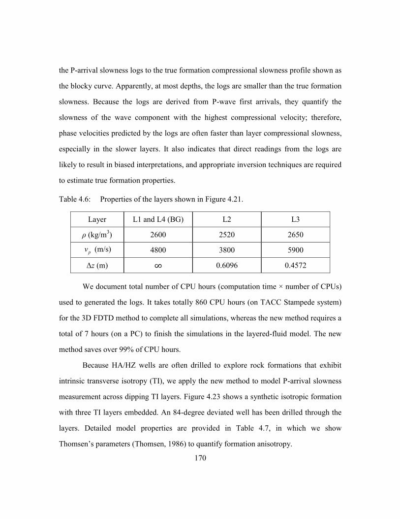
170
the P-arrival slowness logs to the true formation compressional slowness profile shown as
the blocky curve. Apparently, at most depths, the logs are smaller than the true formation
slowness. Because the logs are derived from P-wave first arrivals, they quantify the
slowness of the wave component with the highest compressional velocity; therefore,
phase velocities predicted by the logs are often faster than layer compressional slowness,
especially in the slower layers. It also indicates that direct readings from the logs are
likely to result in biased interpretations, and appropriate inversion techniques are required
to estimate true formation properties.
Table 4.6: Properties of the layers shown in Figure 4.21.
Layer L1 and L4 (BG) L2 L3
ρ (kg/m3) 2600 2520 2650
pv (m/s) 4800 3800 5900
Δz (m) ∞ 0.6096 0.4572
We document total number of CPU hours (computation time × number of CPUs)
used to generated the logs. It takes totally 860 CPU hours (on TACC Stampede system)
for the 3D FDTD method to complete all simulations, whereas the new method requires a
total of 7 hours (on a PC) to finish the simulations in the layered-fluid model. The new
method saves over 99% of CPU hours.
Because HA/HZ wells are often drilled to explore rock formations that exhibit
intrinsic transverse isotropy (TI), we apply the new method to model P-arrival slowness
measurement across dipping TI layers. Figure 4.23 shows a synthetic isotropic formation
with three TI layers embedded. An 84-degree deviated well has been drilled through the
layers. Detailed model properties are provided in Table 4.7, in which we show
Thomsen’s parameters (Thomsen, 1986) to quantify formation anisotropy.

171
Figure 4.22: Comparison of P-arrival slowness logs calculated in the model shown in
Figure 4.21. The blocky line represents the compressional slowness profile
of the rock formations. Slownesses of layers L1 and L4 are labeled as “BG”.
Figure 4.23: Synthetic model consists of an isotropic background and three dipping
layers with TI anisotropy. The well is deviated at 84 degrees.

172
Table 4.7: Properties of the formations shown in Figure 4.23.
Layer BG L1 L2 L3
ρ (kg/m3) 2560 2500 2600 2520
pvv (m/s) 3400 2470 4000 2780
svv (m/s) 1700 1265 2000 1435
ε 0 0.12 0.125 0.1
δ 0 0.08 0.1 0.14
γ 0 0.1 0.11 0.08
Δz (m) ∞ 0.6096 0.4572 0.3962
Figure 4.24: Comparison of P-arrival slowness logs calculated in the model with three
84-degree dipping TI thin beds. The blocky line represents quasi-P slowness
profile of the layers.

173
Each anisotropic layer is modeled as an equivalent isotropic layer, and we assign
quasi-P velocity as the compressional velocity of the layer. Providing the equivalent
isotropic layers, the remaining simulation steps are the same as in the previous example.
Modeled P-arrival slowness logs are shown in Figure 4.24. In the entire logging interval,
the log from rapid modeling agrees with the one from FDTD simulation, with a relative
error less than 4%. As a result of the dominant influence from the fastest layer, L2, the
log slowness values at most depths are smaller than the quasi-P profile, especially in the
slower layers. We conclude from the example that our modeling algorithm is applicable
to estimate P- arrival slowness in thinly bedded TI formations.
In the previous two examples, the wellbore approaches and penetrates the dipping
layers at a fixed angle, and we model P-arrival slowness log in the example with an
undulating trajectory shown in Figure 4.3. The quasi-P velocities previously provided in
Table 4.4 are used as input parameters. Following the same workflow as in the previous
example, we model the TI layers as isotropic ones using their quasi-P velocities. Figure
4.25 shows the results, where we observe that the log obtained using fast-forward
modeling closely approximate the one from FDTD simulations. Maximum relative error
equals 4%. In the meantime, the rapid modeling method reduces the computation time by
99%.

174
Figure 4.25: Comparison of P-arrival slowness logs calculated in the HA well example
with three TI thin beds. The blocky line represents quasi-P slowness values
of the rock formations.
4.9 CONCLUSIONS
When an HA/HZ well penetrates thinly bedded formations, complex geometrical
condition introduces simultaneous excitation of wave modes of different orders.
Interference of the modes results in distortions in frequency-slowness dispersion curve
and inhibits estimation of formation shear slowness from low-frequency asymptote of
flexural mode dispersion. We developed semi-analytical three-dimensional spatial
sensitivity functions for monopole Stoneley and dipole flexural modes in frequency
ranges away from the distortions. Fast forward modeling algorithm based on weighted
integral using the sensitivity functions successfully simulated dispersion logs for the
respective modes obtained in synthetic examples across TI thin beds.
P-mode in HA/HZ wells is also significantly influenced by mode interference
across dipping bed boundaries. As a result, the waveforms registered at the array
receivers show low semblance, and the conventional waveform coherence-based

175
processing method is inadequate to provide reliable compressional slowness estimation.
We introduced P-arrival slowness log that can be obtained from compressional first-
arrivals in HA/HZ wells. P-arrival slowness log measures fastest-traveling converted P-
wave through the formation layers, and is less affected by wave interference.
Accordingly, we developed an equivalent layered model that eliminates borehole-guided
P-waves while retaining the converted ones. The equivalent model reduces the
geometrical complexity from 3D to 1D, and enables us to develop a fast forward
modeling method using real-axis integration method in the f-k domain. In synthetic
examples with high-angle wells penetrating multiple TI thin beds, the modeling algorithm
provides accurate estimation of P-arrival slowness logs, as well as a 99% reduction in
computation time comparing to 3D FDTD method. The P-arrival slowness log and the
corresponding fast-forward modeling approach we introduced suggest the possibility for
developing inversion-based interpretations of sonic logs to provide layer-by-layer
estimations of formation elastic properties in HA/HZ wells.

176
Chapter 5: Summary, Conclusions, and Future Research
Recommendations
This final chapter summarizes the technical contributions made in this dissertation
and presents general conclusions, recommended best practices, and recommendations for
further research.
5.1 SUMMARY
This dissertation presents new research focusing on the responses of borehole
acoustic logging flexural, Stoneley, P-, and S- modes to rock formation elastic property
(shear slowness, compressional slowness, and mass density) perturbations. The goal is to
define and calculate sonic spatial sensitivity functions that quantitatively represent the
volume of investigation of the respective measurements, and to gain insight into borehole
acoustic methods that may be exploited in modeling and inversion of sonic logs. Further
objectives include the development of fast-forward modeling of borehole sonic
dispersions in vertical wells across thinly bedded formations, inversion of available sonic
logs for layer-by-layer estimation of formation elastic properties, and fast simulation of
sonic logs in highly deviated wells.
Accurate and fast forward modeling algorithms that generate synthetic borehole
sonic logs in the presence of geometrical complexity due to thin beds and radial elastic
property alterations have been elusive, which is the main motivation of the first part of
the dissertation. Instead of solving the direct problem using numerical methods, we use
Green’s functions of borehole sonic measurements for fast simulation. We performed
numerical perturbation analysis with respect to formation shear slowness, compressional
slowness, and mass density by introducing perturbed cell into a homogeneous formation.
Numerically simulated spectra in the frequency domain were processed using the WSS

177
method to yield slowness dispersions, from which we calculated the impulse response of
the measurement that maps elastic property perturbations to corresponding measurement
perturbations. The perturbation analysis unmasked axial and axial-radial sensitivity
functions of dipole flexural and monopole Stoneley modes at multiple discrete
frequencies. The sensitivity functions quantify the volume of investigation of the
measurements, which depends on formation elastic properties, dispersion mode,
operating frequency, and tool aperture (length of the receiver array).
As a step further toward improved interpretation of sonic logs in complex
environments, we developed an effective formation model consisting of multiple
horizontal layers such that geometrical complexity associated with the borehole and the
logging tool is eliminated. For a specific mode, at each frequency, the layer properties of
the effective formation are dynamically determined to include the influences of the
borehole fluid, logging tool, and formation. The effective formation approach enables us
to derive semi-analytical formulations for rapid calculation of the sensitivity functions.
The semi-analytically calculated sensitivity functions closely represent the ones obtained
using numerical perturbation analysis.
Considering insight garnered from the sensitivity study, we realized that the
sensitivity functions provide discrete first-order approximations to the Green’s functions
of borehole sonic measurements. The semi-analytical sensitivity functions are useful for
estimating normal mode dispersion in the presence of arbitrarily distributed elastic
heterogeneities. Accordingly, we developed a fast forward-modeling method that
employs the sensitivity functions as weighting filters to integrate elastic property
perturbations in the rock formation surrounding the wellbore. The integral yields
variations in mode dispersion due to the distributed elastic heterogeneities. By adaptively
selecting the reference medium and recalculating the sensitivity functions, we applied the

178
forward-modeling algorithm to generate synthetic multi-frequency dispersion logs of
Stoneley and flexural modes across multiple horizontal thin beds with invasions. We also
extended the method to characterize slownesses of the non-dispersive P- and S-modes in
thinly bedded formations based on an analogy with low-frequency flexural mode
dispersion. The forward modeling algorithm was validated by comparing modeled logs to
numerical simulation results, wherein we quantify relative error and the computation time
reduction of our method.
Providing the fast-forward modeling approach, in the second part of the
dissertation, we introduced an inversion-based workflow for layer-by-layer interpretation
of formation elastic properties. The workflow is applicable for both flexural mode and P-
and S- modes measured in vertical wells across thinly bedded formations. Because of
mode dispersivity, flexural dispersion logs at different frequencies provide independent
measurements that can be jointly used to invert formation shear slowness. Accordingly,
we developed an inversion algorithm to estimate formation shear slowness of each thin
bed from multi-frequency flexural dispersion logs. The cost function was built as the
quadratic difference between the modeled dispersion logs and the flexural mode
dispersion data (from numerical simulations or field measurements). The Levenberg-
Marquardt method was employed to minimize the cost function iteratively with the
Jacobian matrix of the problem numerically calculated using the fast-forward modeling
method. For P- and S-modes, we modified the algorithm to simultaneously solve for
vertical distributions of formation compressional and shear slowness through joint
inversion of P- and S- slowness logs. The joint inversion scheme combines P- and S-
slowness data and builds the cost function in terms of elastic moduli such that the
estimated slownesses are always self-consistent. The inversion method corrects averaging

179
effects introduced by thin beds and shoulders, and we applied it to challenging synthetic
and field cases to verify its reliability and efficiency.
Undulating wells introduce complex geometrical conditions that are adverse for
modeling and interpretation of borehole sonic measurements. The final part of the
dissertation presented numerically simulated sonic measurements in high angle wells
across a dipping shoulder bed, where the contrast in elastic properties between the
formation layer and the shoulder bed is relatively large. From numerical simulations, we
found that the deleterious distortion effect has negligible impact on mid- to high
frequency dispersion, and we developed three-dimensional (axial-radial-azimuthal)
sensitivity functions to model Stoneley and flexural mode dispersions in fast formations,
circumventing multi-mode interference at the low frequencies. We validated the forward-
modeling method for the respective modes at an undulating high angle well that
penetrates multiple thin beds with TI anisotropy. Furthermore, we investigated P-mode in
HA wells and showed that compressional first arrivals are notably less influenced by
mode interference than the late arrivals. Subsequently, we introduced an apparent
slowness log from the P-arrivals, which is more reliable than the conventional P-mode
slowness log calculated using the STC method. Moreover, we developed a semi-
analytical approach for rapidly simulating the P-arrival slowness log. This approach
assumes effective formation layers with no borehole and logging tool, which enables us
to employ the one-dimensional real-axis integration method to predict the log. Using
synthetic cases consisting of undulating wellbore and multiple anisotropic thin beds, we
compared modeled logs to numerically simulated ones and verified the accuracy and the
reduction in computation time of our fast-forward modeling approach.
180
5.2 CONCLUSIONS
This section summarizes the general and specific conclusions stemming from the
research presented in the previous three chapters.
5.2.1 General conclusions about the best practices for petrophysical modeling and
inversion of borehole sonic measurements
i. The main contribution and significance of this dissertation are the development of
spatial sensitivity function-based fast forward modeling and inversion techniques
for improved petrophysical quantification and formation evaluation in thinly
bedded rock formations.
ii. The techniques documented in this dissertation endeavor to maintain
computational efficiency for potential practical usages in modeling and inversion-
based analysis of borehole sonic measurements, to yield high-resolution layer-by-
layer estimation of in-situ formation elastic properties for petrophysical, rock
mechanical, and geophysical applications.
iii. Complex geometrical conditions (e.g., thin beds, mud-filtrate invasion, and
drilling induced damages near the wellbore) induce biasing effects that obscure
true formation elastic properties. Conventional sonic log interpretation relies on
semblance calculation of the array waveforms to calculate formation velocities
without accounting for shoulder-bed and radial alteration effects. Such analysis
introduces significant errors into the subsequent reservoir delineation and reserve
estimation tasks. Thus, business decisions made according to such conventional
analysis are risky and should be considered bad practice.
iv. The sensitivity functions reflect that different formation elastic properties provide
different influences on sonic measurements. Formation shear slowness chiefly
controls dipole flexural and monopole Stoneley mode dispersions, especially at

181
low frequencies (2 to 3 kHz). P- and S- mode propagation properties are
dominantly controlled by formation compressional and shear slownesses,
respectively. It follows that one can only estimate formation shear slowness from
flexural dispersion data, whereas P-mode slowness measurement must be
involved for formation compressional slowness estimation.
v. Theoretically, sensitivity functions can be defined in different domains (e.g.,
velocity, slowness, and elastic modulus). We showed that for sonic logs obtained
using routine processing techniques (the WSS and STC methods), the sensitivity
functions defined in terms of slowness best establish the linearity between a
spatial elastic property perturbation and the corresponding measurement
perturbation.
vi. Because the research is developed according to linear perturbation theory,
accuracy of sensitivity function-based forward modeling is governed by the
choice of the reference homogeneous medium. Selection of a reference medium
and calculation of sensitivity functions need to be conducted adaptively according
to the measured logs, to ensure that the contrast in elastic property between the
reference and the estimation is within the perturbation limit. We showed that a
criterion of 15% variation in shear slowness log is appropriate for adaptive
sensitivity calculations.
vii. It is well known that thin beds and shoulders have the effect of smoothing the logs
because of averaging effects. We found that strong and uneven should-bed effects
can shift or eliminate the bed boundary signatures in sonic logs. Thus,
interpretations made without modeling and inversion are problematic, resulting in
erroneous boundary locations and biased elastic property estimations.
182
viii. Generally, wireline sonic measurements (i.e., Stoneley and flexural mode
dispersions, and P- and S- mode slownesses) exhibit nonlinear response with
respect to spatially distributed formation elastic property variations.
Consequently, the nonlinear minimization method is most appropriate for the
inversion of sonic logs. The gradient-based nonlinear iterative inversion method
we use (i.e., the Levenberg-Marquardt method) is efficient to provide accurate
estimates and to ensure fast convergence.
ix. One factor that contributes to the efficiency of the inversion-based sonic log
interpretation is the stability of inversion results. Stability is investigated with the
speed of convergence to a minimum error. In the course of the research
documented in this dissertation, we found that the L-curve method (Hansen,
2001) was appropriate for selecting the regularization parameter used to stabilize
nonlinear inversion of sonic logs, which is especially important in the first
iteration.
x. Borehole sonic measurements are subject to various kinds of environmental noise.
As a result, measured logs usually contain multiple spikes. Due to the presence of
the spikes, separate inversion of P- and S- mode slowness logs is likely to result in
estimations that are inconsistent the constraint in velocity ratio. A better practice
is to formulate the inversion in terms of elastic moduli such that the velocities
calculated from the moduli strictly satisfy the rock physical constraint.
xi. In HA/HZ wells, geometrical properties becomes three-dimensional due to the
presence of deviated thin beds. Simultaneous excitation of normal modes of
different orders introduces adverse conditions for waveform processing and sonic
log interpretation. The low-frequency part of flexural mode dispersion that is
commonly used to infer formation shear slowness often exhibits large distortions.

183
Shear slowness logs obtained using conventional analysis (i.e., estimated from a
flexural mode low-frequency asymptote) are unreliable in HA/HZ wells. The
forward modeling method using spatial sensitivity functions are appropriate for
modeling flexural mode dispersion at high frequencies, which is useful for
estimating true formation shear slowness.
xii. Across highly deviated thin beds, interference between guided and converted P-
waves introduces phase discontinuity in the waveforms. Waveform semblance-
based methods (e.g., the STC method) are inadequate to provide appropriate P-
mode slowness logs in such a circumstance. In comparison, apparent slowness
logs derived from P-mode first arrival are much less affected by the late-arrival
interference, which is also predictable using the one-dimensional real-axis
integration method. P-arrival slowness logs predicted matches the numerical
simulations within a few percent, suggesting the possibility of inversion-based
analysis of formation compressional slowness in high angle wells.
5.2.2 Spatial sensitivity functions for fast-forward modeling of borehole sonic
measurements
1. Frequency-slowness dispersions of borehole sonic multipole normal modes are
jointly influenced by formation elastic properties, i.e., shear slownesses,
compressional slowness, and mass density. Sensitivity of a particular dispersion
mode is a function of frequency, formation type (fast or slow with respect to
borehole fluid compressional velocity), and receiver array geometry.
2. For the flexural mode, formation shear slowness sensitivity is 10 times more than
the sensitivities to the other properties at low frequency (2 kHz). As frequency
increases to 5 kHz and above, shear slowness sensitivity decreases to 3 to 4 times
the other two types of sensitivities.

184
3. For the Stoneley mode, formation shear slowness also provides the most dominant
influence at low frequencies (2 kHz and below). Low-frequency shear slowness
sensitivity is 4 to 5 times larger than the other two, whereas at higher frequencies,
shear slowness sensitivity decreases and becomes comparable with the other two.
4. Depth of investigation of a specific dispersive mode is frequency dependent,
quantified from the axial-radial shear slowness sensitivity functions. Flexural
mode radial depth of investigation contracts toward the borehole wall as
frequency increases. Its radial depth of investigation equals 0.4 m at 2 kHz, which
decreases to 0.1 m at 7 kHz. Stoneley mode depth of investigation changes from
0.3 m at 1 kHz to 0.1 m at 6 kHz and above. Generally, the Stoneley mode has a
shallower depth of investigation than that of the flexural mode.
5. Forward modeling based on semi-analytical flexural and Stoneley mode
sensitivity functions provides accurate and rapid simulation of dispersion logs at
discrete frequencies. In synthetic verification examples consisting of thin beds
with large elastic property variations (more than 80 us/ft in shear slowness
contrast), the modeled logs agree with simulated ones within 2% and 1% for
flexural and Stoneley modes, respectively. In addition, application of the fast
forward modeling method saves 98% of computation time.
6. In analogy with flexural mode dispersion at the low-frequency asymptote, we
developed semi-analytical axial sensitivity function for P- and S- modes. In
challenging synthetic examples, the logs simulated using the sensitivity functions
have a relative error as low as 4% compared to numerical results. Furthermore,
because the fast forward modeling method removes the need to solve wave
equations, over 99% of computation time is saved.

185
5.2.3 Inversion-based interpretation of borehole sonic logs
i. The first inversion algorithm proposed in the dissertation uses multi-frequency
flexural dispersion data to provide layer-by-layer estimation of shear slowness in
vertical wells when the tool logs in thin-bedded formations. The inversion is
developed using the Levenberg-Marquardt nonlinear minimization method in the
slowness domain, and the dispersion logs at 2 to 6 kHz (with a spacing of 1 kHz)
are employed to construct the quadratic cost function and to suppress uncertainty.
The shear slowness is estimated to within 3% of the true formation property,
accompanied by a maximum uncertainty of 3%.
ii. The joint inversion algorithm introduced in this dissertation combines P- and S-
mode slowness logs measured in vertical wells for simultaneous estimation of
formation compressional and shear slownesses. The algorithm is developed in the
elastic modulus domain to yield slowness estimations consistent with the
constraints in the vp /vs ratio. In synthetic verification examples, estimated
compressional and shear slownesses are accurate with a maximum relative error
of 4% compared to the true model. Without multi-frequency data, the joint
inversion method results in a slightly higher uncertainty of 6%. All vp /vs ratios
derived from the estimated slownesses are consistent with the constraint
2 / 2.5p sv v .
iii. Because the inversion algorithms invoke the fast forward-modeling schemes to
calculate the Jacobian matrix, 99% of CPU time is reduced compared to
numerical simulation methods. Compared to conventional sonic log
interpretations, the algorithms provide improved vertical resolution, from 1.83 m
to 0.5 m, without undermining noise tolerance of the array waveform data.

186
iv. Applications of the joint inversion algorithm to challenging field case examples
verify that the estimations from our method are more accurate than conventional
well-log analysis. Quantitatively, the difference between the measured log and the
estimation indicated that conventional interpretations can introduce a relative
error of 14%.
5.2.4 Fast-forward modeling of dispersion and P-arrival slowness measurements in
HA/HZ wells
i. Presence of deviated thin beds has considerable impact on borehole sonic mode
dispersions. Strong distortions occurred in the flexural mode dispersion curve at
low frequencies, thus inhibiting formation shear slowness estimation. We found
that for fast formations, Stoneley (above 1 kHz) and flexural (above 4 kHz)
dispersions exhibit no distortions. According to the same procedure as in the 2D
case, we developed 3D (axial-radial-azimuthal) semi-analytical sensitivity
functions to model Stoneley and flexural mode dispersions measured in
formations with highly deviated thin beds. Modeled logs (from 4 to 8 kHz and at
1 kHz for flexural mode and Stoneley mode, respectively) have a maximum
relative error of 2% versus numerical simulation results. Compared to 3D finite-
difference simulations, the rapid modeling using 3D sensitivity functions provides
a 99% reduction in CPU time.
ii. The rapid modeling algorithm is useful to predict dispersion measurements in
HA/HZ wells penetrating horizontal thin beds with TI anisotropy. The TI layers
were modeled using equivalent isotropic parameters in wellbore axial direction:
for the flexural mode, we used quasi-velocities; and for Stoneley mode, we used
the equivalent shear velocity given by Chi and Tang (2003).
187
iii. In HA/HZ wells, due to mode conversion and interference in the proximity of the
bed boundaries, P-mode waveforms registered at different receivers exhibit low
semblance, and compressional slowness quantified using STC method depends on
the length of the processing window. Instead of waveform semblance
calculations, from compressional first arrivals, we derived the P-arrival slowness
that is less influenced by late-arrival interference.
iv. We found that P-mode first arrivals in HA/HZ wells are dominantly controlled by
converted P-waves through the dipping formation layers. Consequently, we
developed an effective model consisting of dipping fluid plates to model the
converted P-waves. The model simplifies the geometrical condition from 3D to
1D and enables fast forward modeling of P-arrival slowness measurement.
v. Based on the one-dimensional model, we used real-axis integration method to
generate synthetic waveforms and estimated P-arrival slowness when the tool logs
in an undulating horizontal well across multiple horizontal anisotropic thin beds.
Modeled logs closely approximate the ones obtained using 3D FDTD simulation;
difference in the logs is within 4%. In addition, the modeling algorithm saves
99% of computation time.
5.3 RECOMMENDED BEST PRACTICES
The following summarizes specific best practices on how to appropriately apply
the techniques developed in this dissertation:
i. The spatial sensitivity functions should be calculated using the semi-analytical
approach we developed. Semi-analytical calculation of the sensitivity functions
rules out the instabilities induced by numerical noises, and significantly reduces
computation time.

188
ii. Elastic properties of borehole fluid and the logging instrument are required for the
semi-analytical approach to appropriately include borehole and tool effects. Tool
properties we suggested can be found in Tables 2.2 and 4.2, and borehole fluid
velocity can be found in measured data, e.g., parameter DTMD is included in
Sonic Scanner data to record mud slowness.
iii. Because the sensitivity functions are developed on the basis of perturbation
theory, adaptive calculation of sensitivity function according to measured
slowness logs is required to ensure no violation of the perturbation assumption.
We recommend monitoring the variation in shear slowness log: if the relative
difference in slowness exceeds 15%, new reference medium needs to be selected
for re-calculation of sensitivity functions.
iv. Due to environmental noise, measured sonic logs often show spikes.
Consequently, separate inversion of a spiky P- or S- mode slowness log is likely
to result in estimates that are inconsistent with the rock physical bounds in
velocity ratio ( 2 / 2.5p sv v ). Joint inversion that combines both P- and S-
mode slowness logs is required to ensure self-consistency in the estimates.
v. Selection of the regularization parameter, α, is the key to ensure stability of the
inversion algorithms. For the inversion technique introduced in this dissertation,
we recommend sweeping through values 0.1 1000 and crossplot the model
norm and the norm of data misfit. The parameter value that gives the solution
closest to the corner of the crossplot should be selected.
vi. Because sonic logs have a vertical resolution lower than other measurements,
when applying the inversion algorithms to field data, one needs to jointly define
the bed boundaries according to sonic and other well logs (e.g., resistivity image,
gamma ray, and density logs).

189
vii. The inversion-based interpretation algorithm implemented in this dissertation
assumes marginal invasion; such an assumption is not warranted in analysis of
severely invaded formations. When the thin beds are subject to radial alterations,
axial-radial sensitivity functions are useful to simulate borehole sonic
measurements.
viii. The three-dimensional semi-analytical sensitivity functions are useful to
simulated high-frequency normal mode dispersions. To avoid the distortion
effects near flexural mode low-frequency asymptote, we suggest using the
sensitivity functions to model the dispersions at 4 kHz and above.
ix. Due to simultaneous excitation of multiple normal modes in HA/HZ wells, for
dispersion analysis, we suggest using the single mode search dispersion analysis
(e.g., Hua and Sarkar, 1990) to find the dispersion of the most dominant mode.
x. Layer-by-layer interpretation of formation elastic properties in HA/HZ wells is
challenging due to the limitations in conventional processing techniques, which
hardly take into account multi-mode interference. Instead of calculating waveform
semblance, we recommend deriving P-arrival slowness log from compressional
first arrivals. Because the first arrivals are much less contaminated by the
interference than the late-arrival wave packets, P-arrival slowness log has better
reliability than the logs from conventional processing.
5.4 FUTURE RESEARCH RECOMMENDATIONS
The following is a list of recommendations that could advance the research topics
documented in this dissertation:
i. The semi-analytical sensitivity functions introduced in this dissertation are
developed for wireline sonic logging normal modes. The basis of the sensitivity

190
functions, i.e., the perturbation theory, however, is not limited to a particular
logging tool. The semi-analytical sensitivity functions could be extended to
describe the propagation properties of monopole and quadruple modes for logging
while drilling (LWD) measurements. Because a typical LWD tool has a shorter
receiver array than the wireline tool assumed in this research, the LWD sensitivity
functions are equivalent to sub-array applications adapted from the wireline ones.
ii. The second-order quadruple mode is occasionally used in LWD measurements to
avoid low-frequency collar mode; the sensitivity function could be applied to
describe propagation properties of the mode based on accurate analytical solution
of the dispersion curve.
iii. The inversion-based method assumes that the formation layers are isotropic. In
vertical wells, when a thin bed has a TI anisotropy resulting from fine
laminations, governed by measurement physics, dipole flexural mode can only
respond to vertical shear velocity. In this case the low-frequency parts (below 2
kHz) of the Stoneley mode are dominantly influenced by horizontal shear velocity
(Tang and Cheng, 2004). The numerical perturbation analysis and the semi-
analytical approach introduced in this dissertation could be adapted to study the
sensitivity of two anisotropic shear velocities for a TI medium. The subsequent
sensitivity functions could be utilized for simultaneous inversion of flexural and
Stoneley dispersions to estimate the shear velocities and the corresponding
anisotropic parameter.
iv. The sensitivity functions show that flexural and Stoneley modes exhibit
frequency-dependent volume of investigation, which could be used to provide
radial profiling of elastic properties in thinly bedded formations with radial
alterations. Because the degree of freedom of the problem increases, assimilating

191
other borehole measurements that are able to detect radial alterations (e.g., array
induction and density logs) as additionally constraints improves inversion
efficiency and accuracy of the estimations.
v. Fast-forward modeling of P-arrival slowness log developed in this dissertation
could be applied for the inversion of formation compressional slowness in highly-
deviated thin beds by matching the simulated log with the one derived from
measured waveforms.
vi. Theoretically, propagation properties of borehole sonic waves are controlled by
formation velocities. Apparent S-arrival slowness log could be estimated using an
adequately defined shear slowness model. The same forward modeling technique
developed for deriving P-arrival slowness can be applied for S-arrival slowness
prediction by substituting layer shear slowness into the integration equations.
Additional challenges could be expected in shear slowness arrival detection due to
the presence of compressional late arrivals.
vii. Forward modeling of high-frequency flexural mode dispersion in HA/HZ wells
could be employed in conjunction with azimuthal processing method (i.e., instead
of taking differences, process the waveforms registered at only one azimuthal
sector of receiver array) to develop a reliable elastic property estimation approach.
Because high-frequency flexural mode dispersion asymptotes to the Scholte wave
velocity, the measurement sensitivity to formation properties is relatively low. In
such a circumstance, reliable formation property estimation could be achieved
with the implementation of non-gradient based methods. Such methods include
Bayesian inversion (Yang and Torres-Verdín, 2013) and derivative-free
algorithms (Aster et al., 2005).

192
List of Symbols
* Complex conjugation
T Transposition
Tensor product
α Regularization parameter
β Noise percentage parameter
ε, δ, γ Thomsen parameters
ε Error vector from WSS processing
θ Azimutal direction (rad)
θ Dip angle, phase angle between wellbore and TI axis of symmetry
λ Lame’s first constant (GPa)
μ Shear modulus (GPa)
ρ Mass density (kg/m3)
ω Angular frequency (rad/s)
[ ]IJc Stiffness tensor of the perturbed formation (GPa)
,[ ]IJ rc Stiffness tensor of the reference formation (GPa)
[ ]IJc Difference between the reference formation stiffness tensor and the
perturbed formation one (GPa)
A Amplitude of source direction radiation
B Amplitude of the down-going wave in the bottom layer in the layered
formation
33c , 44c ,
66c Stiffness tensor elements
C Amplitude of the up-going wave in the middle layer in the layered
formation

193
C Cost function
d Data vector
dP Data vector consists of P-mode slowness
dS Data vector consists of S-mode slowness
D Amplitude of the down-going wave in the middle layer in the layered
formation
e Misfit between modeled and observed data
E Amplitude of the up-going wave in the top layer in the layered
formation
f Frequency (kHz)
G Spatial sensitivity function
G(m) Measurement system
,a rG Semi-analytical radial sensitivity
,a zG Semi-analytical axial sensitivity
Ga,θ Semi-analytical azimuthal sensitivity
,a r zG Semi-analytical axial-radial sensitivity
,a r zG Semi-analytical axial-radial-azimuthal sensitivity
h Amplitude of a particular mode
I Identity matrix
J Jacobian matrix
k Wavenumber of the modal wave in the reference formation (rad/m)
k’ Wavenumber of the modal wave in the perturbed formation (rad/m)
kx Wavenumber parallel with bed boundaries (rad/m)
kcn Wavenumber in n-th layer perpendicular to bed boundaries (rad/m)
L First modulus that equals 2 22p sv v 2 2(m /s )

194
L’ Equivalent moduli of the perturbed formation (GPa)
m Model parameters
m The receiver index corresponding to the perturbed layer
mi The i-th parameter
Δm The vector that determines the direction toward convergence at the end
of the each iteration
Mr Elastic property of the background medium
ΔM Spatial distributions of elastic properties in rocks surrounding the
borehole
ΔM/Mr Elastic heterogeneity function
N Total number of receivers
n Index of an arbitrary receiver
qP Quasi compressional velocity
qSV Quasi shear vertical
r Radial direction (m)
Δr Radial thickness of a perturbed cell (m)
s Dispersion mode slowness of the perturbed formation (us/ft)
s0 Estimated mode slowness from the WSS method (us/ft)
sj The j-th data point
ps Compressional slowness
sr Dispersion mode slowness of the reference formation (us/ft)
ss Shear slowness
Δs Slowness variation of a particular dispersion mode (us/ft)
T Center of processing window
Tw Length of processing window
U Second modulus that equals 2 2 2 (m /s )sv

195
V Volume of consideration (m3)
pv Compressional velocity
pvv Vertical compressional velocity
sv Shear velocity
,s STv Equivalent shear velocity for Stoneley mode
svv Vertical shear velocity
X Modal wave spectrum
Xn Modal wave spectrum at the n-th receiver
Z Measured phase delay across the receiver array (rad)
Z0 Phase delay across the receiver array given by the WSS method (rad)
z Vertical direction (m)
zL Lower boundary location of the perturbed layer (m)
zU
Upper boundary location of the perturbed layer (m)
Δz Vertical thickness of a perturbed layer/cell (m)

196
List of Acronyms
1D One-Dimensional
2D Two-Dimensional
3D Three-Dimensional
BG Background
CPU Central Processing Unit
cm Centimeter
ft Foot
FE Finite Element
FDTD Finite Difference Time Domain
GPa Giga Pascal
HA High Angle
HZ Horizontal
in Inch
kHz Kilohertz
kg/m3 Kilogram per cubic meter
Ln Layer n
m Meter
MPa Mega Pascal
MD Measured Depth
P- Compressional
PC Personal Computer
S- Shear
STC Slowness-Time Coherence
TI Transverse Isotropy

197
us/ft Microsecond per foot
WSS Weight Spectrum Semblance
TVD True Vertical Depth

198
References
Aki, K., and P. G. Richards, 2002, Quantitative seismology, 2nd Edition: University
Science Books.
Al-Chalabi, M., 1994, Seismic velocities - a critique: First Break, 12, no.12, 589–596.
Alumbaugh, D., and X. Lu, 2001, Three-dimensional sensitivity analysis of induction
logging in anisotropic media: Petrophysics, 42, no. 6, 566–579.
Alumbaugh, D., and M. Wilt, 2001, A numerical sensitivity study of three dimensional
imaging from a single borehole: Petrophysics, 42, no. 1, 19–31.
Aster, R., B. Borchers, and C. Thurber, 2005, Parameter estimation and inverse problems:
Elsevier Academic.
Backus, G. E., 1962, Long-wave elastic anisotropy produced by horizontal layering,
Journal of Geophysical Research, 67, no. 11, 4427–4440.
Bassiounimore, Z., 1994, Theory, measurement, and interpretation of well logs: Society
of Petroleum Engineers Textbook Series, 4.
Biryukov, S.V., Y. V. Gulyaev, V. Krylov, and V. Plessky, 1995, Surface acoustic waves
in inhomogeneous media: Springer Series on Wave Phenomena, 20.
Born, M., and E. Wolf, 1965, Principles of optics, 3rd edition: Pergamon Press.
Burridge, R., and B. Sinha, 1996, Inversion for formation shear modulus and radial depth
of investigation using borehole flexural waves: 66th Annual International
Meeting, SEG, Expanded Abstracts, 158–161.
Cerveny, V., 2001, Seismic ray theory: Cambridge University Press.
Cheng, C. H., and M. N. Toksöz, 1981, Elastic wave propagation in a fluid‐filled
borehole and synthetic acoustic logs: Geophysics, 46, no. 7, 1042–1053.
Chi, S. H., and X. M. Tang, 2003, Accurate approximations to qsv and qp wave speeds in
TIV media and Stoneley wave speed in general anisotropic media:. Transactions
of the Society of Petrophysicists and Well Log Analysts, 48th Annual Logging
Symposium, paper OO.
Chi, S., C. Torres-Verdín, J. Wu, and O. F. Alpak, 2004, Assessment of mud-filtrate
invasion effects on borehole acoustic logs and radial profiling of formation elastic
paramters: Society of Petroleum Engineers Annual Technical Conference and
Exhibition Proceedings, SPE 90159.
Coates, R., M. Kane, C. Chang, C. Esmersoy, M. Fukuhara, and H. Yamamoto, 2000,
Single-well sonic imaging: high-definition reservoir cross-sections from
horizontal wells: Society of Petroleum Engineers/Canadian Institute of Mining
International Conference on Horizontal Well Technology, SPE/Petroleum Society
of CIM 65457.
199
Ellefsen, K. J., C. H. Cheng, and M. N. Toksöz, 1999, Applications of perturbation
theory to acoustic logging: Journal of Geophysical Research, 96, no. B1, 537–
549.
Fedorov, F. I., 1968, Theory of elastic Waves in crystals: Plenum Press.
Gelinsky, S., and X. Tang, 1997, Fast forward modeling of Stoneley waves for irregular
boreholes and heterogeneous formations: 67th Annual International Meeting,
SEG, Expanded Abstracts, 317–320.
Han, D., 1992. Fluid saturation effect on rock velocities in seismic frequencies: Presented
at the SEG-EAEG Summer Research Workshop.
Hansen, P. C., 1998, Rank-deficient and discrete ill-posed problems: numerical aspects of
linear inversion: Society of Industrial and Applied Mathematics Monographs on
Mathematical Modeling and Computation.
Hansen, P. C., 2001, The L-Curve and its use in the numerical treatment of inverse
problems, in P. R. Johnston, eds., Computational Inverse Problems in
Electrocardiography, 119–142.
Heidari, Z., C. Torres-Verdín, A. Mendoza, O. Ijasan, and B. Voss, 2009, Rapid,
interactive assessment of petrophysical and geometrical effects on density and
neutron logs acquired in vertical and deviated wells: Society of Petroleum
Engineers Annual Technical Conference and Exhibition Proceedings, SPE
124879.
Hauser, J., M. Sambridge, and N. Rawlinson, 2008, Multi-arrival wavefront tracking and
its applications: Geochemistry, Geophysics, Geosystems, 9, no. 11.
Huang, S., Matuszyk, P. J., and Torres-Verdín, C., 2013, Spatial Sensitivity Functions for
Rapid and Accurate Simulation of Borehole Sonic Measurements: 83th Annual
International Meeting, SEG, Expanded Abstracts, 509–513.
Huang, S., P. J. Matuszyk, and C. Torres-Verdín, 2015, Spatial sensitivity functions for
rapid simulation of borehole sonic measurements in vertical wells, in minor
revision.
Hudson, J. A., and J. R. Heritage, 1981, The use of the Born approximation in seismic
scattering problems: Geophysical Journal International, 66, no. 1, 221–240.
Hsu, K., and S. K. Chang, 1987, Multiple-shot processing of array sonic waveforms for
high resolution sonic logs: GEOPHYSICS, 52, no. 10, 1376–1390.
Ijasan, O., C. Torres-Verdín, and W. E. Preeg, 2013, Inversion-based petrophysical
interpretation of logging-while-drilling nuclear and resistivity measurements:
GEOPHYSICS, 78, no. 6, D473–D489.
Kazatchenko, E., M. Markov, and A. Mousatov, 2003, Determination of primary and
secondary porosity in carbonate formations using acoustic data: Society of

200
Petroleum Engineers Annual Technical Conference and Exhibition, SPE-84209-
MS.
Kimball, C. V., and T. L. Marzetta, 1986, Semblance processing of borehole acoustic
array data: GEOPHYSICS, 49, 274–281.
Lin, S., W. C. Hsieh, Y. C. Lim, T. F. Yang, C. S. Liu, and Y. Wang, 2006: Methane
migration and its influence on sulfate reduction in the good weather ridge region,
South China Sea continental margin sediments: Terrestrial, Atmospheric and
Oceanic Sciences, 17, no. 4, 883–902.
Lindsay, R. and R. Van Koughnet, 2001, Sequential Backus averaging: upscaling well
logs to seismic wavelengths: The Leading Edge, 20, no. 2, 188–191.
Liu, Z., C. Torres-Verdín, G. L. Wang, A. Mendoza, and P. Zhu, 2007, Joint inversion of
density and resistivity logs for the improved petrophysical assessment of thinly-
bedded clastic rock formations: Transactions of the Society of Petrophysicists and
Well Log Analysts, 48th Annual Logging Symposium, paper VV.
Mallan, R., J. Ma, C. Torres-Verdín, and G. L. Wang, 2009, Joint radial inversion of
resistivity and sonic logs to estimate in-situ petrophysical and elastic properties of
formations: Society of Petroleum Engineers Annual Technical Conference and
Exhibition, SPE 124624.
Matuszyk, P. J., L. Demkowicz, and C. Torres-Verdín, 2012, Solution of coupled
acoustic-elastic wave propagation problems with anelastic attenuation using
automatic hp-adaptivity: Computer Methods in Applied Mechanics and
Engineering, 213–216, 299–313.
Matuszyk, P. J., and L. Demkowicz, 2014, Solution of coupled poroelastic-acoustic-
elastic wave propagation problems using automatic hp-adaptivity: Computer
Methods in Applied Mechanics and Engineering, 281, 54–80.
Matuszyk, P. J., C. Torres-Verdín, and D. Pardo, 2013, Frequency-domain finite-element
simulations of 2D sonic wireline borehole measurements acquired in fractured
and thinly bedded formations: GEOPHYSICS 78, no. 4, D193–D207.
Mavko, G., T. Mukerji, and J. Dvorkin, 2003, The rock physics handbook, 2nd Edition:
Cambridge University Press.
Mendoza, A., C. Torres-Verdín, and W. E. Preeg, 2007, Rapid simulation of borehole
nuclear measurements based on spatial flux-scattering functions: Transactions of
the Society of Petrophysicists and Well Log Analysts, 48th Annual Logging
Symposium, paper O.
Mendoza, A., C. Torres-Verdín, and W. E. Preeg, 2010a, Linear iterative refinement
method for the rapid simulation of borehole nuclear measurements: Part 1 –
Vertical wells: GEOPHYSICS, 75, no. 1, E9–E29.

201
Mendoza, A., C. Torres-Verdín, and W. E. Preeg, 2010b, Linear iterative refinement
method for the rapid simulation of borehole nuclear measurements: Part 2 – High-
angle and horizontal wells: GEOPHYSICS, 75, no. 2, E79–E90.
Montmayeur, H. and R. M. Graves, 1985, Prediction of static elastic/mechanical
properties of consolidated and unconsolidated sands from acoustic measurements:
basic measurements: Society of Petroleum Engineers Annual Technical
Conference and Exhibition, SPE-14159-MS.
Mosca, I., and J. Trampert, 2009, Path-average kernels for long wavelength traveltime
tomography: Geophysical Journal International, 177, 639–650.
Mukhanov, V. F., H. A. Feldman, and R. H. Brandenberger, 1992, Theory of
cosmological perturbations. Part 1. Classical perturbations. Part 2. Quantum
theory of perturbations. Part 3. Extensions: Physics Report, 215, 203–333.
Mukhanov, V. F., 2005, Physical foundations of cosmology: Cambridge University Press.
Musgrave, M. J. P., 1970, Crystal acoustics: Holden-Day.
Nolte, B., and Huang, X., 1997, Dispersion analysis of split flexural waves: Annual
report of borehole acoustics and logging and reservoir delineation consortia,
Massachusetts Institute of Technology.
Oyler, D. C., C. Mark, and G. M. Molinda, 2008, Correlation of sonic travel time to the
uniaxial compressive strength of U.S. coal measure rocks: Proceedings of the 27th
International Conference on Ground Control in Mining.
Peyret, A., and C. Torres-Verdín, 2006, Assessment of shoulder-bed, invasion, and
lamination effects on borehole sonic logs: a numerical sensitivity study:
Transactions of Society of Petrophysicists and Well Log Analysts, 47th Annual
Logging Symposium, paper PP.
Passey, Q. R., H. Yin, C. M. Rendeiro, and D. E. Fitz, 2005, Overview of high-angle and
horizontal well formation evaluation – Issues, learnings, and future directions:
Transactions of the Society of Petrophysicists and Well Log Analysts, 46th
Annual Logging Symposium, paper A.
Pistre, V., T. Kinoshita, T. Endo, K. Schilling, J. Pabon, B. Sinha, T. Plona, T. Ikegami,
and D. Johnson, 2005, A modular wireline sonic tool for measurements of 3D
(azimuthal, radial, and axial) formation acoustic properties: Transactions of
Society of Petrophysicists and Well Log Analysts, 46th Annual Logging
Symposium, paper P.
Rendeiro, C., Q. R., Passey, and H. Yin, 2005, The conundrum of formation evaluation in
high-angle and horizontal wells – Observations and recommendations: Society of
Petroleum Engineers Annual Technical Conference and Exhibition Proceedings, SPE
96898.
202
Rosenbaum, J. H., 1974, Synthetic micro-seismograms: logging in porous formations:
GEOPHYSICS, 39, 14–32.
Sanchez-Ramirez, J., C. Torres-Verdín, D. Wolf, G. L. Wang, A. Mendoza, Z. Liu and G.
Schell, 2010, Field examples of the combined petrophysical inversion of gamma-
ray, density, and resistivity logs acquired in thinly-bedded clastic rock formations:
Petrophysics, 51, no. 4, 247–263.
Schmitt, D. P., M. Bouchon, and G. Bonnet, 1988, Full waveform synthetic acoustic logs
in radially semi-infinite saturated porous media: GEOPHYSICS, 53, 807–823.
Schmidt, H., and G. Tango, 1986, Efficient global matrix approach to the computation of
synthetic seismograms: Geophysical Journal of the Royal Astronomical Society,
84, no. 2, 331–359.
Sinha, B. K., 1997, Sensitivity and inversion of borehole flexural dispersions for
formation parameters: Geophysical Journal International, 128, 84–96.
Sinha, B., and S. Kostek, 1996, Stress‐induced azimuthal anisotropy in borehole flexural
waves: GEOPHYSICS, 61, no. 6, 1899–1907.
Sinha, B., B. Vissapragada, L. Renlie, and S. Tysse, 2006, Radial profiling of the three
formation shear moduli and its application to well completions: GEOPHYSICS, 71,
no. 6, E65–E77.
Stark, P., and D. Nikolayev, 1993, Toward tubular tomography: Journal of Geophysical
Research, 98, 8095–8106.
Tang, X., and A. Cheng, 2004, Quantitative borehole acoustic methods: Pergamon Press.
Tang, X., N. Cheng, and A. Cheng, 1999, Identifying and estimating formation stress
from borehole monopole and cross-dipole acoustic measurement: Transactions of
the Society of Petrophysicists and Well Log Analysts, 40th Annual Logging
Symposium, paper QQ.
Thomsen, L., 1986, Weak elastic anisotropy: GEOPHYSICS, 51, no. 10, 1954–1966.
Torres-Verdín, C., and T. Habashy, 2001, Rapid 2.5‐dimensional forward modeling and
inversion via a new nonlinear scattering approximation: Radio Science, 29, no. 4,
1051–1079.
Tsang, L., and D. Rader, 1979, Numerical evaluation of the transient acoustic waveform
due to a point source in a fluid-filled borehole: GEOPHYSICS, 44, 1706–1720.
Tubman, K., C. H. Cheng, and M. N. Toksöz, 1986, Synthetic full waveform acoustic
logs in cased boreholes II: Poorly bonded casing, GEOPHYSICS, 51, 902–913.
Walls, J. D., 1987, Poisson’s ratio and mechanical properties from core and well log
measurements, Society of Petroleum Engineers Annual Technical Conference and
Exhibition, SPE-16795-MS.

203
Winkler, K., B. Sinha, and T. Plona, 1998, Effects of borehole stress concentrations on
dipole anisotropy measurements: GEOPHYSICS, 63, 11–17.
Wyllie, M. R. J., A. R. Gregory, and L. W. Gardner, 1956, Elastic wave velocities in
heterogeneous and porous media: GEOPHYSICS, 21, 41–70.
Yang, Q. and C. Torres-Verdín, 2013, Joint stochastic interpretation of conventional well
logs acquired in hydrocarbon-bearing shale: Transactions of the Society of
Petrophysicists and Well Log Analysts, 54th Annual Logging Symposium.
Zhang, T., X. M. Tang, and D. Patterson, 2000, Evaluation of laminated thin beds in
formations using high-resolution acoustic slowness logs: Transactions of the
Society of Petrophysicists and Well Log Analysts, 41st Annual Logging
Symposium, paper XX.

204
Vita
Shan Huang received the Bachelor of Engineering degree in Electronic
Engineering (2001) and the Master of Engineering degree in Electronic Science and
Technology (2004) from Tsinghua University, P. R. China. During 2004-2009, he
worked for Schlumberger Beijing Geoscience Center (Beijing, P. R. China) as a project
engineer. He entered the doctoral program in 2010 at the Department of Petroleum and
Geosystems Engineering of The University of Texas at Austin.
Permanent email address: [email protected]
This dissertation was typed by Shan Huang.
Recommended