
University of California
Los Angeles
Coordinated Actuation
for Sensing Uncertainty Reduction
A dissertation submitted in partial satisfaction
of the requirements for the degree
Doctor of Philosophy in Electrical Engineering
by
Aman Kansal
2006

c© Copyright by
Aman Kansal
2006
The dissertation of Aman Kansal is approved.
Gaurav S. Sukhatme
Deborah Estrin
William J. Kaiser
Gregory J. Pottie, Committee Co-chair
Mani B. Srivastava, Committee Co-chair
University of California, Los Angeles
2006
ii
Table of Contents
1 Introduction . . . . . . . . . . . . . . . . . . . . . . . . . . . . . . . . 1
1.1 Key Contributions . . . . . . . . . . . . . . . . . . . . . . . . . . 5
1.2 Related Contributions . . . . . . . . . . . . . . . . . . . . . . . . 8
1.3 Prototype system . . . . . . . . . . . . . . . . . . . . . . . . . . . 9
1.4 Outline . . . . . . . . . . . . . . . . . . . . . . . . . . . . . . . . . 10
2 Related Work . . . . . . . . . . . . . . . . . . . . . . . . . . . . . . . 11
2.1 Estimation Theoretic Optimization . . . . . . . . . . . . . . . . . 11
2.2 Geometric Optimization . . . . . . . . . . . . . . . . . . . . . . . 13
2.3 Control Theoretic Methods . . . . . . . . . . . . . . . . . . . . . . 15
2.4 Other Optimization Methods . . . . . . . . . . . . . . . . . . . . 16
2.5 Active Cameras . . . . . . . . . . . . . . . . . . . . . . . . . . . . 19
2.6 Other Related Work . . . . . . . . . . . . . . . . . . . . . . . . . 22
3 Sensing Advantages of Small Motion . . . . . . . . . . . . . . . . 24
3.1 Small Motion On Infrastructure . . . . . . . . . . . . . . . . . . . 24
3.1.1 Single Obstacle Model . . . . . . . . . . . . . . . . . . . . 25
3.1.2 Multiple Obstacles . . . . . . . . . . . . . . . . . . . . . . 28
3.1.3 Experiments . . . . . . . . . . . . . . . . . . . . . . . . . . 31
3.1.4 Two-dimensional Motion on Infrastructure . . . . . . . . . 38
3.2 Pan, Tilt, and Zoom Motion for Cameras . . . . . . . . . . . . . . 39
3.2.1 Usable Range of PZT Motion . . . . . . . . . . . . . . . . 44
iii

3.2.2 Advantage with Multiple Nodes . . . . . . . . . . . . . . . 46
3.3 Trade-offs in Using Small Motion . . . . . . . . . . . . . . . . . . 48
3.3.1 Feasible Resolution . . . . . . . . . . . . . . . . . . . . . . 49
3.3.2 System Deployment and Operation Cost . . . . . . . . . . 51
3.3.3 Actuation Delay . . . . . . . . . . . . . . . . . . . . . . . . 55
4 System Architecture . . . . . . . . . . . . . . . . . . . . . . . . . . 57
4.1 Technology Context . . . . . . . . . . . . . . . . . . . . . . . . . . 62
5 Motion Coordination Methods . . . . . . . . . . . . . . . . . . . . 64
5.1 Sensing Performance . . . . . . . . . . . . . . . . . . . . . . . . . 64
5.1.1 Actuation Delay . . . . . . . . . . . . . . . . . . . . . . . . 65
5.1.2 Detection Performance . . . . . . . . . . . . . . . . . . . . 66
5.1.3 Performance Objective . . . . . . . . . . . . . . . . . . . . 66
5.2 Distributed Motion Coordination . . . . . . . . . . . . . . . . . . 68
5.2.1 Complexity Considerations . . . . . . . . . . . . . . . . . . 68
5.2.2 A Distributed Approach . . . . . . . . . . . . . . . . . . . 69
5.2.3 Coordination Algorithm . . . . . . . . . . . . . . . . . . . 71
5.3 Convergence and Other Properties of the Motion Coordination
Algorithm . . . . . . . . . . . . . . . . . . . . . . . . . . . . . . . 74
5.3.1 Graceful Degradation . . . . . . . . . . . . . . . . . . . . . 77
5.3.2 Relationship to Other Heuristics . . . . . . . . . . . . . . . 77
5.4 Coordination Protocol Implementation . . . . . . . . . . . . . . . 79
5.4.1 Protocol Specification . . . . . . . . . . . . . . . . . . . . 79
iv

6 Medium Mapping and Phenomenon Detection . . . . . . . . . . 85
6.1 Medium Mapping . . . . . . . . . . . . . . . . . . . . . . . . . . . 85
6.1.1 Enabling Self-Awareness . . . . . . . . . . . . . . . . . . . 87
6.1.2 System Design Issues . . . . . . . . . . . . . . . . . . . . . 90
6.1.3 Adaptive Medium Mapping . . . . . . . . . . . . . . . . . 94
6.1.4 Reducing the Scan Time . . . . . . . . . . . . . . . . . . . 98
6.1.5 Algorithm Implementation and Evaluation . . . . . . . . . 101
6.1.6 Sharing the Self-awareness Data . . . . . . . . . . . . . . . 107
6.1.7 Related Work . . . . . . . . . . . . . . . . . . . . . . . . . 114
6.2 Phenomenon Detection . . . . . . . . . . . . . . . . . . . . . . . . 115
6.2.1 Ellipse Detection . . . . . . . . . . . . . . . . . . . . . . . 116
6.2.2 Color Detection . . . . . . . . . . . . . . . . . . . . . . . . 117
6.2.3 Motion Detection . . . . . . . . . . . . . . . . . . . . . . . 118
7 Simulations, Prototype, and Experiments . . . . . . . . . . . . . 124
7.1 Simulations . . . . . . . . . . . . . . . . . . . . . . . . . . . . . . 124
7.1.1 Accuracy of Converged State . . . . . . . . . . . . . . . . 127
7.1.2 Convergence Speed . . . . . . . . . . . . . . . . . . . . . . 130
7.2 Prototype System . . . . . . . . . . . . . . . . . . . . . . . . . . . 132
7.3 Experimental Evaluation . . . . . . . . . . . . . . . . . . . . . . . 135
8 Conclusions and Future Work . . . . . . . . . . . . . . . . . . . . . 145
8.1 Future Directions . . . . . . . . . . . . . . . . . . . . . . . . . . . 147
v

References . . . . . . . . . . . . . . . . . . . . . . . . . . . . . . . . . . . 149
vi

List of Figures
1.1 Resolution determines feasible data processing. . . . . . . . . . . . 3
1.2 Protypte system with motile cameras and supporting resources. . 9
3.1 Abstract obstacle model for analytical calculation of coverage. . . 25
3.2 Calculating the advantage due to mobility for a simplified obstacle
model. . . . . . . . . . . . . . . . . . . . . . . . . . . . . . . . . . 28
3.3 Sample obstacles in deployment terrain (The small line along the
lower edge shows the track on which the sensor moves). . . . . . . 30
3.4 Coverage with varying obstacle density, with and without mobility.
The error bars show the variance among 20 runs with different
random obstacle placements. . . . . . . . . . . . . . . . . . . . . . 31
3.5 Actuation advantage (multiplicative reduction in probability of
mis-detection) in varying obstacle density. . . . . . . . . . . . . . 32
3.6 Actuation advantage (multiplicative reduction in probability of
mis-detection) with varying obstacle size. . . . . . . . . . . . . . . 33
3.7 The laboratory test-bed for testing coverage advantage due to mo-
bility. . . . . . . . . . . . . . . . . . . . . . . . . . . . . . . . . . . 34
3.8 The coordinates of trees from Wind River forest [Win03] used to
place the obstacles in laboratory test-bed. . . . . . . . . . . . . . 34
3.9 Probability of Mis-detection in laboratory test-bed experiments:
varying number of cameras. PoM is lower with mobility. . . . . . 36
3.10 Image of real world scene showing obstacles consisting of trees and
foliage, among which the target is to be detected. . . . . . . . . . 37
vii

3.11 NIMS-LS: a system to provide infrastructure supported 2D motion. 38
3.12 Nitrate concentration (mg/l) across the cross-section of a river. . . 39
3.13 Actuation in a PZT camera (a) volume covered without actuation
can be modeled as pyramid, (b) tilt capability increases the ef-
fective volume covered, (c) combined pan and zoom capabilities
further increase the volume covered, and (d) volume covered when
pan, tilt, and zoom are combined: this can be viewed as a portion
of a sphere swept out using pan and tilt, where the thickness of
the sphere depends on the zoom range. . . . . . . . . . . . . . . . 41
3.14 (a) Covered volumes for detection and sensing phases, with the
pan, tilt, and zoom required to provide sensing resolution within
the detection volume. (b) The time to change zoom measured as
a function of the zoom step. The communication delay in sending
the zoom command was separately characterized and has been
subtracted from the motion time. . . . . . . . . . . . . . . . . . . 45
3.15 Evaluating coverage gain due to motion with varying actuation
delay and difference in detection and identification resolution. . . 46
3.16 Instantaneous coverage increase: (a) a sample topology showing
randomly oriented sensors, and (b) sensor orientations changed
using pan capability. . . . . . . . . . . . . . . . . . . . . . . . . . 47
3.17 Coverage advantage when pan actuation is used for initial recon-
figuration only, at multiple densities. Error bars show standard
deviation across 10 random topologies. (Node density is measured
as the number of sensors in the area covered by a single sensor.) . 48
viii

3.18 Alternative deployments: Coverage fraction with and without ac-
tuation at different deployment densities. Node density is the num-
ber of nodes in a 20m×20m square region, where each sensor covers
a sector of 45◦ with radius Rs = 7.3m. The error bars show the
standard deviation across 10 random topologies simulated. . . . . 53
3.19 Converting the node density to total network cost, at 90% coverage
point. . . . . . . . . . . . . . . . . . . . . . . . . . . . . . . . . . 55
4.1 System software architecture. . . . . . . . . . . . . . . . . . . . . 60
5.1 Illustrative scenario for motion coordination algorithm. The white
cirular regions are obstacles. The darker shade is uncovered region.
The lighter shaded regions represent covered areas, where lighter
regions represent better detection. . . . . . . . . . . . . . . . . . . 73
5.2 Utility function for various possible pan pose combinations. The
θp values are in degrees, measured counter-clockwise from initial
camera pose. The utility function has multiple local maxima, even
for this simple scenario. . . . . . . . . . . . . . . . . . . . . . . . . 74
6.1 System architecture, consisting of self-awareness and application
sensors. . . . . . . . . . . . . . . . . . . . . . . . . . . . . . . . . 88
6.2 Prototype self-awareness node. . . . . . . . . . . . . . . . . . . . . 90
6.3 Map generation process. . . . . . . . . . . . . . . . . . . . . . . . 96
6.4 Varying spatial resolution with obstacle distance. . . . . . . . . . 101
6.5 Adaptive step size control algorithm for medium mapping. . . . . 102
6.6 Comparing the number of readings taken with varying error per-
formance for the three scanning strategies. . . . . . . . . . . . . . 105
ix

6.7 Comparing the adaptive and periodic scan strategies using the
prototype self-awareness node. . . . . . . . . . . . . . . . . . . . . 106
6.8 Range coordinates used to compute occupancy grids (OG’s) . . . 108
6.9 Example: Generating a combined OG directly at the application
sensor. . . . . . . . . . . . . . . . . . . . . . . . . . . . . . . . . . 109
6.10 Comparison of data size for multiple storage strategies, with vary-
ing scan error. . . . . . . . . . . . . . . . . . . . . . . . . . . . . . 111
6.11 Example visual tag used for object detection. . . . . . . . . . . . 116
6.12 Detecting regions of interest using motion detection. . . . . . . . . 120
6.13 Differencing to detect pixels which change. . . . . . . . . . . . . . 121
6.14 Filtering motion events of interest for phenomenon detection. . . . 122
7.1 Illustration of ILS convergence (a) random initial network config-
uration (b) optimized configuration with w = 0.1, showing signifi-
cantly improved coverage than (a). . . . . . . . . . . . . . . . . . 125
7.2 Illustration of ILS: optimized coverage using w = 0.9, showing a
different stable state. . . . . . . . . . . . . . . . . . . . . . . . . . 126
7.3 Illustration of ILS (a) a sample event distribution, where brighter
areas show higher event density (b) optimized configuration after
learning the event distribution, and (c) optimized configuration
with α set to a high value. . . . . . . . . . . . . . . . . . . . . . . 127
7.4 Optimization accuracy: convergence with ten random search paths.
Each curve shows a different random contention success pattern.
The various converged states have a utility within 10.9% of the
best case. . . . . . . . . . . . . . . . . . . . . . . . . . . . . . . . 129
x

7.5 Convergence: evolution of utility with increasing number of itera-
tions. Each curve corresponds to a random location topology and
random initial poses of the sensors. . . . . . . . . . . . . . . . . . 130
7.6 Gathering medium information for ILS operation (a) range scan
from laser in bottom left corner (b) range scan from laser in top
right corner, (c) map of obstacles in the medium and the initial
network configuration, (d) optimized configuration found by ILS
- it changes both the pan and zoom settings of the cameras to
increase sensing performance characterized by time required for
recognition. . . . . . . . . . . . . . . . . . . . . . . . . . . . . . . 133
7.7 GUI snapshots of the four processes controlling the network cam-
eras in the testbed. . . . . . . . . . . . . . . . . . . . . . . . . . . 135
7.8 Experiment monitoring software. . . . . . . . . . . . . . . . . . . 136
7.9 System software in operation alongside the testbed. . . . . . . . . 137
7.10 Event trace . . . . . . . . . . . . . . . . . . . . . . . . . . . . . . 139
7.11 Performance of different network configurations, when optimiza-
tion is weighted for actuation delay. . . . . . . . . . . . . . . . . . 141
7.12 Utility metric evaluated for various configurations. . . . . . . . . . 142
7.13 Performance of different network configurations, when configura-
tion optimization is weighted for detection performance. . . . . . 143
7.14 Utility metric for various configurations, when detection perfor-
mance is weighted higher. . . . . . . . . . . . . . . . . . . . . . . 144
xi

List of Tables
3.1 Mis-detection probabilities with and without motion for real-world
experiment . . . . . . . . . . . . . . . . . . . . . . . . . . . . . . . 37
3.2 Example actuation specifications, for camera used in prototype,
Sony SNC RZ30N. . . . . . . . . . . . . . . . . . . . . . . . . . . 40
3.3 Coverage Improvement with PZT actuation . . . . . . . . . . . . 43
6.1 Algorith parameter values. . . . . . . . . . . . . . . . . . . . . . . 103
7.1 Required actuation ranges and hardware capabilities. . . . . . . . 138
xii

Acknowledgments
The work in this dissertation was facilitated by the efforts of several people, be-
ginning first and foremost with my co-advisers Prof Mani B Srivastava and Prof
Gregory J Pottie. I am grateful to Prof Srivastava for not only providing starting
directions in the basic problem space explored in this dissertation but significant
help in shaping the specifics of the problem addressed. His constant encour-
agement and flexibility in exploring risky off-shoots of the primary hypothesis
provided for a very exciting and enjoyable research environment for my thesis
research. I am also thankful to Prof Pottie for his constant feedback and the
wider perspective on modeling the relevant factors in the problems studied. The
extensive collaborative opportunities provided by him for exploring fundamental
problems in sensing with collaboration among multiple sensors and information
theoretic considerations were also very beneficial in pursuing my research objec-
tives. The significant advice received from both my advisers in the domains of
technical writing and accurate expression of the research findings are also worthy
of acknowledgment.
I am also grateful to my thesis committee members Prof Deborah Estrin, Prof
William Kaiser, and Prof Gaurav Sukhatme. Their continued feedback has gone
beyond an external evaluation of the work and has provided me with valuable
suggestions and a deeper understanding of the issues explored.
I have been fortunate that this work was also supported by the Networked
Infomechanical Systems (NIMS) project at Center for Embedded Networked Sens-
ing (CENS) at UCLA. The efforts by NIMS team members on various related
aspects of the problems addressed in this thesis provided a richer understanding
and wider applicability for the work.
xiii

I am also indebted to my student collaborator James Carwana for the several
lengthy experiments designed, developed, and executed with me for one of the
modules of the system developed as part of this dissertation. I also wish to thank
Eric Yuen and Michael Stealey for their efforts on some of the initial experimental
studies for this dissertation. I further acknowledge the efforts of other students
who worked with me on several problems in controllably mobile sensor networks
that are related to, though not covered in, this dissertation, including Arun So-
masundara, Jonathan Friedman, David Lee, Parixit Aghera, and Advait Dixit. I
am also grateful to several others who collaborated on multiple complimentary
problems in sensor networks, including Jason Hsu, Sadaf Zahedi, Ameesh Pandya,
Mohammad Rahimi, Aditya Ramamoorthy, Richard Pon, Maxim Batalin, Duo
Liu, Vijay Raghunathan, Dunny Potter, Saurabh Ganeriwal, and David Jea.
A special note of thanks is also due to my undergraduate advisers Prof Uday
Desai, Prof Abhay Karandikar, and Prof Rakesh Lal who introduced me to ad-
vanced research in networking, wireless communication, and embedded networks
for the first time. Gratitude is also due to Rick Baer at Agilent Technologies
for the valuable exposure to practical system development issues and in-depth
insights into the behavior of cameras and other technology components used in
this dissertation.
I would also like to thank the faculty at University of California Los Angeles
who have contributed greatly to my education including Prof Michael Fitz, Prof
Adnan Darwiche, Prof Mario Gerla, Prof Izhak Rubin, and Prof Kung Yao.
The work for this dissertation was carried out at the Networked and Em-
bedded Systems Laboratory (NESL) at the Electrical Engineering Department,
UCLA and I am grateful to the several members of NESL, including but not lim-
ited to Vlasios Tsiatsis, Andreas Savvides, Ramkumar Rengaswamy, Roy Shea,
xiv

Heemin Park, Laura Balzano, and Simon Han, for helping in various forms in-
cluding the numerous discussions held at NESL, assistance with equipment issues,
sharing opinions and philosophical insights on issues in my research area, and last
but not the least for fueling excitement about sensor networks.
I express my deepest gratitude to my parents, Vandana and Devinder Kansal,
for their constant support and love. Their extremely valuable contributions to my
initial education and an early exposure to the scientific process were instrumental
in my research pursuits. I am also grateful to my wife, Vasudha Kaushik, for her
support and tolerance.
This research was supported in part by the National Science Foundation
(NSF) under Grant Nos. ANI-00331481 and 0306408, the Center for Embedded
Networked Sensing (CENS) at University of California Los Angeles, the Office
of Naval Research (ONR) under the AINS program, and the DARPA PAC/C
program.
xv

Vita
1979 Born, Patiala, Punjab, India.
2001 B. Tech., Electrical Engineering
Indian Institute of Technology Bombay
Mumbai, India.
2001-2002 Teaching Assistant, Department of Electrical Engineering, IIT
Bombay. Courses: EE 421 Communication System Theory, and
EE 764 Wireless and Mobile Communications.
2002 M. Tech., Communications and Signal Processing
Indian Institute of Technology Bombay
Mumbai, India.
2002 University of California Regents Fellowship, Department of
Electrical Engineering, University of California Los Angeles.
2003-2005 Graduate Student Researcher, Networked and Embedded Sys-
tems Laboratory, Department of Electrical Engineering, Uni-
versity of California Los Angeles.
2005 Summer Intern, Agilent Labs, Palo Alto, California.
2005-2006 Graduate Student Researcher, Networked and Embedded Sys-
tems Laboratory, Department of Electrical Engineering, Uni-
versity of California Los Angeles.
2006 – Researcher, Microsoft Research.
xvi

Publications
MA Batalin, M Rahimi, Y Yu, D Liu, A Kansal, G Sukhatme, W Kaiser, M
Hansen, G Pottie, MB Srivastava, and D Estrin. Call and Response: Experiments
in Sampling the Environment. In Proceedings of ACM Sensys, November 3-5,
2004, Baltimore, MD.
S Ganeriwal, A Kansal and MB Srivastava. Self-aware Actuation for Fault Re-
pair in Sensor Networks. In Proceedings of IEEE International Conference on
Robotics and Automation (ICRA) April 26 - May 1, 2004, New Orleans, LA.
J Hsu, S Zahedi, A Kansal, MB Srivastava. Adaptive Duty Cycling for En-
ergy Harvesting Systems. ACM-IEEE International Symposium on Low Power
Electronics and Design (ISLPED), October 4-6, 2006, Tegernsee, Germany.
J Hsu, S Zahedi, D Lee, J Friedman, A Kansal, V Raghunathan, and MB Sri-
vastava. Demo Abstract: Heliomote: Enabling Long-Lived Sensor Networks
Through Solar Energy Harvesting. In Proceedings of ACM Sensys, November
2-4, 2005, San Diego, CA.
A Kansal, J Carwana, WJ Kaiser, and MB Srivastava. Demo Abstract: Coor-
dinating Camera Motion for Sensing Uncertainty Reduction. In Proceedings of
ACM Sensys, November 2-4, 2005, San Diego, CA.
A Kansal, J Carwana, WJ Kaiser, and MB Srivastava. Acquiring Medium Models
xvii

for Sensing Performance Estimation. In Proceedings of IEEE SECON, September
26-29, 2005, Santa Clara, CA.
A Kansal and UB Desai. Motion Constraint Based Handoff Protocol for Mobile
Internet. In Proceedings of IEEE Wireless Communications and Networking
Conference (WCNC), March 16-20, 2003, New Orleans, LA.
A Kansal and UB Desai. Handoff Protocol for Bluetooth Public Access. In Pro-
ceedings of IEEE International Conference on Personal Wireless Communications
(ICPWC), December 15-17, 2002, New Delhi, India.
A Kansal and UB Desai. A rapid handoff protocol for mobility in Bluetooth
public access networks. In Proceedings of the Fifteenth International Conference
on Computer Communication, August 2002, Mumbai, India.
A Kansal and UB Desai. Mobility support for Bluetooth public access. In Pro-
ceedings of IEEE International Symposium on Circuits and Systems (ISCAS),
May 26-29, 2002, Phoenix, AZ.
A Kansal, J Hsu, MB Srivastava, V Raghunathan. Harvesting Aware Power
Management for Sensor Networks. In Proceedings of the 43rd Design Automation
Conference (DAC), July 24-28, 2006, San Fransisco, CA.
A Kansal, W Kaiser, G Pottie, MB Srivastava, and G Sukhatme. Virtual High
Resolution for Sensor Networks. In Proceedings of ACM SenSys, November 1-3,
2006, Boulder, CO.
xviii
A Kansal and A Karandikar. An Overview of Delay Jitter Control for Packet
Audio in IP-Telephony. In IETE Technical Review, Vol. 20, No. 4, July-August
2003.
A Kansal and A Karandikar. Adaptive delay adjustment for low jitter audio
over Internet. In Proceedings of IEEE Globecom, November 25-29, 2001, San
Antonio, TX.
A Kansal and A Karandikar. Jitter free Audio Playout over Best Effort Packet
Networks. In Proceedings of ATM Forum International Symposium on Broad-
band Communication in the New Millennium, August 2001, New Delhi, India.
A Kansal, D Potter and MB Srivastava. Performance Aware Tasking for Environ-
mentally Powered Sensor Networks. In Proceedings of ACM Joint International
Conference on Measurement and Modeling of Computer Systems (SIGMETRICS)
June 12-16, 2004, New York, NY.
A Kansal, M Rahimi, WJ Kaiser, MB Srivastava, GJ Pottie, and D Estrin.
Controlled Mobility for Sustainable Wireless Networks. In Proceedings of IEEE
Sensor and Ad Hoc Communications and Networks (SECON) October 4-7, 2004,
Santa Clara, CA.
A Kansal, A Ramamoorthy, GJ Pottie, MB Srivastava. On sensor Network Life-
time and Data Distortion. In Proceedings of IEEE International Symposium on
Information Theory (ISIT), September 4-9, 2005, Adelaide, Australia.
xix

A Kansal and MB Srivastava. Distributed Energy Harvesting for Energy Neutral
Sensor Networks. In IEEE Pervasive Computing, Vol 4, No. 1, January-March
2005.
A Kansal and MB Srivastava. Energy Harvesting Aware Power Management.
Book Chapter, in Wireless Sensor Networks: A Systems Perspective,Eds. N
Bulusu and S Jha, Artech House, 2005.
A Kansal, A Somasundara, D Jea, MB Srivastava, and D Estrin. Intelligent Fluid
Infrastructure for Embedded Networks. In Proceedings of ACM International
Conference on Mobile Systems, Applications and Services (MobiSys), June 6-9,
2004, Boston, MA.
A Kansal and MB Srivastava. An Environmental Energy Harvesting Framework
for Sensor Networks. In Proceedings of ACM/IEEE Int’l Symposium on Low
Power Electronics and Design (ISLPED), August 25-27, 2003, Seoul Korea.
A Kansal, L Xiao, and F Zhao. Relevance Metrics for Coverage Extension Us-
ing Community Collected Cell-phone Camera Imagery. In Proceedings of ACM
SenSys Workshop on World-Sensor-Web: Mobile Device Centric Sensor Networks
and Applications, October 31, 2006, Boulder, CO.
A Kansal, E Yuen, WJ Kaiser, G Pottie and MB Srivastava. Sensing Uncertainty
Reduction Using Low Complexity Actuation. In Proceedings of ACM Third
International Symposium on Information Processing in Sensor Networks (IPSN)
April 26-27, 2004, Palo Alto, CA.
xx

A Pandya, A Kansal, GJ Pottie, and MB Srivastava. Lossy Source Coding of
Multiple Gaussian Sources: m-helper problem. In Proceedings of IEEE Informa-
tion Theory Workshop (ITW) October 24-29, 2004, San Antonio, TX.
A Pandya, A Kansal, GJ Pottie, and MB Srivastava. Fidelity and Resource Sensi-
tive Data Gathering. In Proceedings of the 42nd Allerton Conference, September
8-12, 2004, Allerton, IL.
xxi

Abstract of the Dissertation
Coordinated Actuation
for Sensing Uncertainty Reduction
by
Aman Kansal
Doctor of Philosophy in Electrical Engineering
University of California, Los Angeles, 2006
Professor Mani B. Srivastava, Co-chair
Professor Gregory J. Pottie, Co-chair
The quality of data returned by a senor network is a crucial parameter of perfor-
mance since it governs the range of applications that are feasible to be developed
using that network. Higher resolution data, in most situations, enables more ap-
plications and improves the reliability of existing ones. In this thesis we discuss
methods that use controlled motion to increase the image resolution in a network
of cameras. In our prototype system, our methods can provide up to 15000x
advantage in resolution, depending on tolerable trade-offs in sensing delay.
Mobility itself may have a high resource overhead, and hence a constrained
form of mobility is exploited, which has low overheads but provides significant
reconfiguration potential. Specifically, we concentrate on pan, tilt, and zoom
motion for cameras. Other forms of constrained motion are also mentioned.
An architecture that allows each node in the network to learn the medium
and phenomenon characteristics is presented. A quantitative metric for sensing
performance is defined based on real sensor and medium characteristics. The
xxii

problem of determining the desirable network configuration is expressed as an
optimization of this metric. A distributed optimization algorithm is developed to
compute a desirable network configuration and adapt it to environmental changes.
A key property of our algorithm is that convergence to a desirable config-
uration can be proved even though no global coordination is involved. Other
desirable properties of the algorithm, such as convergence accuracy and conver-
gence time are also studied. Its relationship to previously known optimization
heuristics is also discussed.
A network protocol to implement this algorithm is discussed for execution in
a totally distributed manner. The protocol involves exchanging messages only in
a well-defined neighborhood.
We evaluate our methods using simulations and experiments on our prototype
system. Real world data is used for testing the algorithm.
xxiii

CHAPTER 1
Introduction
Several research efforts [SS02, PK00, EGH00b, RAS00, SS03, SMP01a, SMP01b]
have established the feasibility of compact, wireless and low energy devices for
sensor networks. A wide range of applications have been prototyped using such
systems in education [SMP01a, SS03], science [CEE01, MPS02], arts and enter-
tainment [BMK02] and defense [MSL04]. In this work we consider the funda-
mental functionality used by all the above applications – sensing the application
specific phenomenon in the deployment environment. Unlike traditional com-
puting systems, sensor networks must deal with complex and inherently noisy
inputs from the physical world. A given application needs a certain sensing per-
formance, which must be guaranteed in the face of unpredictable phenomenon
distributions and the presence of static and mobile environmental obstacles. The
system designer is challenged to not only provide the required performance within
the resource constraints of embedded sensor nodes and a limited power budget
but also ensure autonomous operation of the system in unknown environments.
Environment specific customization is not desirable, as it hinders rapid deploy-
ment. Our objective is to develop methods for understanding and controlling the
uncertainty in the sensed data.
For instance, in the case of image data, the data uncertainty may be related
to the resolution at which the desired space is covered. This spatial resolution
may determine if a desired application can be realized or not using the network.
1

Higher resolution may enable newer applications. Higher resolution also helps re-
duce the effect of transducer noise since more pixels may be allocated to the same
spatial region. Suppose the density at which the cameras are deployed and the
image resolution of each camera is such that a unit length in real space, placed
at any point in the area covered by the network, maps to P pixels in the image.
Then, we define the coverage resolution1 as Ppixels/m. Different points in the
covered area may be at different distances from the respective nearest camera
and coverage resolution may be defined to be that provided at the worst case
point covered by the network. Figure 1.1(a) shows an example scene desired to
be covered by a camera network. Suppose the image data is to be used by a
sensor network application interested in photographing the vehicles in the scene.
A small portion of the scene where a vehicle is present is shown at 15pixels/m
resolution in Fig. 1.1(b). This resolution may be sufficient for applications in-
terested in detecting vehicles, such as using motion detection, in the scene but
not for applications interested in recognizing the vehicles. Figure 1.1(c) shows2 a
small section of the same field of view with the coverage resolution increased to
200pixels/m. Such a resolution may enable an application that is interested in
recognizing the vehicles present in the scene. The simple example clearly shows
that increasing the resolution may enable newer applications. Given a finite set of
sensing resources, it is thus important to provide the highest coverage resolution
feasible with those resources.
There are many ways in which the resolution may be improved. Given the fea-
sible maximum sensor density, signal processing may be used to combine images
1Pixels on some sensing devices may be rectangular rather than square making a unit lengthin space map to different number of pixels depending on whether the length is consideredaligned horizontally or vertically. For such devices, we arbitrarily choose to align the unitlength horizontally for defining coverage resolution.
2The image resolution in the printed paper may vary from the resolution of image data usedin the figure.
2
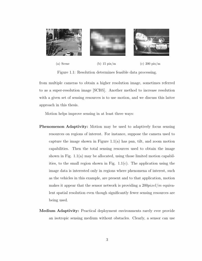
(a) Scene (b) 15 pix/m (c) 200 pix/m
Figure 1.1: Resolution determines feasible data processing.
from multiple cameras to obtain a higher resolution image, sometimes referred
to as a super-resolution image [SCI05]. Another method to increase resolution
with a given set of sensing resources is to use motion, and we discuss this latter
approach in this thesis.
Motion helps improve sensing in at least three ways:
Phenomenon Adaptivity: Motion may be used to adaptively focus sensing
resources on regions of interest. For instance, suppose the camera used to
capture the image shown in Figure 1.1(a) has pan, tilt, and zoom motion
capabilities. Then the total sensing resources used to obtain the image
shown in Fig. 1.1(a) may be allocated, using those limited motion capabil-
ities, to the small region shown in Fig. 1.1(c). The application using the
image data is interested only in regions where phenomena of interest, such
as the vehicles in this example, are present and to that application, motion
makes it appear that the sensor network is providing a 200pixel/m equiva-
lent spatial resolution even though significantly fewer sensing resources are
being used.
Medium Adaptivity: Practical deployment environments rarely ever provide
an isotropic sensing medium without obstacles. Clearly, a sensor can use
3

motion to reduce the occlusions to its view due to obstacles in the medium.
Such use of motion assumes that the sensor can obtain information about
the obstacles, either from its own data or through external means. Further,
when multiple sensors are present they may use motion to minimize overlap
areas among their coverage, and hence potentially focus on smaller regions,
providing a high resolution coverage within those smaller regions.
Increased Sensor Range: Mobile sensors can patrol a larger volume, depend-
ing on the acceptable motion delay.
Motion itself may have a high resource overhead but the sensing advantages
often outweigh the cost of motion for appropriate system design choices. To
this end, we focus our discussion on a specific type of motion capability in the
cameras, namely the ability to pan, tilt, and zoom. Such cameras are sometimes
referred to as active cameras in computer vision or motile sensors3 in robotics.
There are several reasons which motivate us to restrict to this type of motion:
1. The navigational overheads of such constrained motion and very low com-
pared to navigating an unconstrained mobile robot, which requires signifi-
cant hardware and software resource overheads.
2. The energy requirements for constrained motion are lower than uncon-
strained mobility since the bulkier components such as the battery, motors
and processing platform can stay stationary while only the transducer has
to move.
3. Such motion is feasible in tethered nodes such as high bandwidth video
sensors where wireless communication may limit data quality.
3The terms motility and mobility are used differently in biology literature and we will notconsider that usage here.
4

4. If the tolerable delay in sensing is small, then only a limited range of mo-
tion may be feasible within the actuation time allowed and small motion
capabilities are sufficient to exploit the delay available.
5. In certain applications the intrusion into user space due to unconstrained
mobile nodes may not be acceptable while small motion such as pan, tilt,
and zoom can be incorporated with negligible intrusion.
We also discuss some other forms of constrained, low-overhead motion modalities.
An interesting analogy of using motion to leverage limited sensing resources
occurs in human eyes. The resolution is highest in the center of the retina and
gradually degrades toward the periphery [PG02]. This is an attempt to minimize
sensing resources (in this case, neurons) and at the same time maximize spatial
resolution and field of view. Rapid eye movements are used to shift the focus of
attention toward a peripheral region when some event, such as motion, is detected
by the low resolution peripheral view [BRD05].
1.1 Key Contributions
The goal of this work is to explore the issues in system design when motion is
used for reducing sensing uncertainty in a sensor network. A review of the prior
work reveals that the approach proposed in this paper has not been considered
before for providing high-resolution coverage.
First, we discuss if and when it helps to use motion as opposed to alternative
methods, such as, using a higher density of static sensors to improve the resolu-
tion at which the area of interest is covered. We focus specifically on constrained
motion with low resource overheads and discuss why and when this particular
form of motion is preferred over other alternatives. We discuss the trade-offs
5

involved, such as the time it takes for the motion actuators to provide the virtual
high-resolution coverage. We systematically characterize this time as the actua-
tion delay, which is a crucial design parameter, and we discuss it in depth. Some
of the work that lead to the findings in this regard was performed in collaboration
and is available in [KYK04] and [KKP04].
Second, we discuss a system architecture which modularizes the various func-
tions of the motion coordination task. A constrained form of mobility is used,
to minimize the resource cost of motion itself. The system architecture describes
the various components required to effectively use motion capabilities.
Third, we develop a motion coordination algorithm that helps use motion
capabilities with low delay. For this objective, we design a realistic sensing per-
formance metric that models the actual coverage characteristics of the sensors,
rather than relying on abstract disk based models. The motion coordination
problem is expressed as an optimization of this metric over various possible node
poses and orientations. Our distributed algorithm optimizes this global metric
using only local communication in a well defined neighborhood. This allows scal-
ability in the number of nodes and reduces the computational complexity of the
optimization.
Fourth, we discuss some desirable properties of our proposed algorithm. We
prove that our distributed algorithm converges to a desirable network configu-
ration. Convergence is proved without assumptions on the differentiability or
smoothness of the performance metric, but the nature of its dependence on sen-
sors is exploited. This is important because the realistic camera coverage model,
along with the presence of obstacles in the medium, does not yield a closed form
expression for the objective function, and it is not immediately obvious if typical
optimization procedures will converge when used with this function.
6

Fifth, we present a network protocol that implements our distributed motion
control algorithm, and addresses practical details such as the message passing
required for local coordination, and the termination of the motion without global
coordination. The effect of environment dynamics on the motion strategy is
considered. The performance of the protocol is studied through simulations that
model multiple sensor network deployments with obstacles.
Sixth, we develop practical methods to provide information about the de-
ployment environment that may further enhance the operation of our motion
coordination algorithm, such as the distribution of the sensed phenomenon over
space in the region being covered and the presence of obstacles that affect sen-
sor range. The methods to collect information about obstacles use laser ranging
from multiple nodes and aggregate the laser data to produce accurate medium
maps that are useful not only for our motion coordination algorithm but may be
applied to other sensor networks for characterizing the quality of coverage. The
laser ranging and mapping methods result from collaborative work described in
[KCK05a].
Finally, we design and implement a network of cameras with limited mobility,
and supporting resources used to learn the presence of obstacles in the medium.
We present an implementation of our proposed methods on this sensor network,
and evaluate the performance of our proposed methods using real world data
from our prototype system. Evaluations are performed in the context of practical
applications which may be realized using our system. Our results indicate that
the proposals in this work can help attain sensing at a previously unachievable
resolution using available sensing resources.
7

1.2 Related Contributions
In addition to the above, some additional issues were explored involving the use
of controlled motion in sensor networks and the reduction of uncertainty using
collaboration among multiple sensors.
Apart from the benefits in sensing performance, controlled motion can also
be used to enhance the communication performance in certain situations. Large
amounts of delay tolerant data can be transferred using a mobile robot rather
than wireless transmission. This is advantageous in terms of energy since it re-
duces the number of hops required and saves the energy spent by embedded
energy constrained nodes for forwarding traffic along multi-hop routes. Addi-
tional advantages occur because the energy spent by the mobile node can even
be replenished at a charging dock while the energy reserves of the sensor nodes
embedded in the sensed environment may be hard to replenish. The analysis of
the exact energy advantage was carried out in the collaborative work, available
in [SKJ06]. The related system design issues such as the appropriate sleep man-
agement and routing protocols, along with a prototype implementation were also
described in [SKJ06].
As mentioned before, the use of controlled motion is only one of the meth-
ods for improving sensing performance and other methods may be applied for
the same objective as well. We also explored the benefits in sensing achievable
though a fusion of data generated at multiple sensor nodes observing a distributed
phenomenon. The results indicate that a lower distortion can be achieved with
a given network throughput if the same throughput is shared among multiple
sensors rather than used by a single sensor. The precise analysis along with the
phenomenon model used and the quantitative analysis of the feasible distortion
advantage is available in [PKP04].
8

1.3 Prototype system
The algorithms and methods discussed in this paper are developed in the context
of a network of cameras with limited motion capabilities, or motility.
The sensed data consists of video streams from these cameras, which are
processed frame by frame to detect events of interest. Detected events are then
sensed at high resolution to provide higher fidelity data for more sophisticated
data processing algorithms, such as those for recognition or classification of the
events. The medium contains physical obstacles that cause occlusions in the
covered region.
The lab scale test-bed is shown in Figure 1.2. Apart from the cameras, it also
has other supporting resources such as medium mapping sensors and processing
platforms.
Figure 1.2: Protypte system with motile cameras and supporting resources.
We also used our prototype system to collect data outside the laboratory
9
setting, in an outdoor environment in the context of a more realistic application
as discussed in a chapter 7.
1.4 Outline
This dissertation is organized as follows. The next chapter summarizes the prior
work that is related to the considerations in our thesis. Chapter 3 discusses the
potential sensing advantage from various types of constrained motion. Chapter
4 describes the design of the overall system architecture and various components
used in realizing the advantages due to motion. Chapters 5 and 6 discuss the key
components of the system architecture in greater detail, including the motion co-
ordination algorithm developed. Chapter 7 describes the simulations, our system
prototype, and the experiments performed to evaluate our proposals. Chapter 8
concludes the dissertation.
10
CHAPTER 2
Related Work
While there is little work on the problem of using motile sensors for improving the
sensing uncertainty and coverage performance of sensor networks, several related
problems have been explored. In this chapter, we summarize prior efforts from a
variety of fields including computer vision, robotics and sensor networks in the
general area of motion coordination for improving coverage related performance
metrics.
The use of motion to enhance coverage in sensor networks has been considered
in other works such as [WR05]; however, random motion was considered instead
of controlled motion. Several motion coordination and configuration strategies
have been explored using controlled motion for coverage and sensing uncertainty
related performance. We study several of these here, and classify them by the type
of algorithm used. This helps us clearly identify the commonalities and differences
in the various approaches, and to exploit their salient features in designing the
algorithms proposed for the specific reconfiguration problem of interest to us.
2.1 Estimation Theoretic Optimization
Some of the motion control methods utilize estimation performance or informa-
tion theory based metrics to model the desired objective functions which are then
optimized for, using analytical or numerical optimization methods.
11

An information theoretic measure of sensing uncertainty was used in [Gro02,
GMK03]. A utility function was defined using an information measure of the
sensor reading and was maximized with respect to the possible set of sensor
motion choices. Numerical methods were used for optimization because the cost
function lead to non-linear constraints. For deriving a distributed method the
utility function was defined as a sum of the individual utilities at each node and
a coupling term. One such coupling was through computing a global feature
state information metric at all nodes, which depends on receiving all the other
nodes’ information metrics. The computational cost of such an approach must
be carefully considered, since it can be a limiting factor for large scale embedded
implementations with constrained processing capabilities. Also, while sharing a
global state may be required for optimal coordination, this may not be feasible
in large scale networks.
Another information measure was defined in [ZSR02] for quantifying the track-
ing performance. Rather than motion control, the utility metric was used for
selecting the next best sensor based on the observations collected up to the cur-
rent time. The information gain was measured using the Mahanalobis distance
between the sensor location and estimated target location, which requires the co-
variance in target estimate from each potential sensor for evaluation. An alterna-
tive was also suggested for non-Gaussian cases when the probability distribution
cannot be represented in parametric form, similar to the particle filter approach:
the distribution of the next sensor reading was simulated using the sensor model
and the current belief about target state. The simulated distribution was used
for computing the entropy or other information measures for all possible sen-
sor choices. Since the selection was limited to neighboring sensors, the method
became inherently distributed; a single sensor was assumed to be tracking the
target at any time and hence collaboration was limited. Other information or
12
estimation variance based cost functions have also been considered for tracking
purposes, such as in [GJ96].
An alternative information measure is the Fischer Information Matrix, and
has also been used, such as, in [AMB05]. A distributed solution was derived
when sensors move on the boundary of the target region for a distance dependent
sensor model. The algorithm resulted in each sensor moving toward the mid-
point of its Voronoi segment. Conditions for convergence of this algorithm were
also presented.
2.2 Geometric Optimization
These methods exploit geometric optimization and computational geometry tools
to model the sensor properties and performance criteria. The optimization cri-
terion is typically a geometric property such as area covered by a sensor or a
specific geometric model for camera visibility.
Several camera placement strategies, also modeled as variants of the Art
Gallery Problem [Chv75, OR87, Fis78], have been studied using these techniques.
The problem is essentially to place omni-directional sensors with infinite range
such that all points in the required region are covered by at least some sensor.
The case where sensors are allowed to move is known as the Watchmen Tours
problem and has also been explored [CNN93, EGH00a, GLL99, LLG97]. Sev-
eral results on polygon covering for different classes of polygons and algorithms
to centrally compute the best coverings are presented in [Nil94]. Further, the
abstract polygon models are extended to more realistic camera coverage models
in [ES04]. A model for camera coverage is taken in terms of its depth of field
and angular field of view. The pan motion is modeled by considering the angular
13

positions that may be reached from any initial pan-angle within a time constraint
T . An optimization problem is then formulated to determine the minimum num-
ber of cameras required to satisfy the coverage constraints and a computation-
ally tractable procedure to solve the optimization problem in 2D is proposed.
However, the procedure is centralized and works only for simple polygons, i.e.,
polygons without holes, since linear time algorithms are available to find the vis-
ible subregion of a simple polygon [GA81] (coverage regions with obstacles are
thus not addressed). A variant which does consider occlusions appears in [CD00].
The coverage at a point due to a single camera is characterized in terms of the
target density at that point, the resolution at which the point is covered and the
probability of the point being occluded due to obstacles. The optimization prob-
lem is centralized and since the exact solution is computationally intractable, an
existing evolutionary algorithm based heuristic is used. In [Suj02], a heuristic
cost function is assigned which accounts for probabilistic information about oc-
clusions, and camera visibility of known target locations. This cost function is
optimized over all possible camera positions. This method is not distributed and
the position is computed at each camera individually.
Some distributed geometric methods were surveyed in [CMB05]. Briefly, the
coverage at a point was modeled as a function of the distance from the sensor
which best covered this point (typically the nearest sensor, but may vary based
on coverage function used), and the total coverage was defined as a weighted in-
tegral of the coverage at all points, the weights being based on a density function
supported over the region of interest. Alternate cost functions for visibility based
coverage (independent of distance within region of visibility) and some other coor-
dination tasks were also discussed. The network configuration was then computed
to optimize the chosen cost function. The interesting step in this optimization
was that for certain cost functions, the gradient turned out to be spatially distrib-
14

uted over a well-chosen proximity graph. Some relevant proximity graphs from
computational geometry were considered, such as the Voronoi and Delaunay re-
lations. This allowed finding local optima using methods distributed over that
proximity graph. The cost functions chosen lead to analytically tractable gra-
dient computation and hence numerical optimization was not required. Specific
examples of this approach may be found in [CMB04, OM04] among others.
2.3 Control Theoretic Methods
These methods draw from the analytical tools of control theory to ensure the
stability and convergence properties, detecting reachability of certain states and
detecting deadlock states of such algorithms. Simple control laws are typically
used based on intuitive heuristics for achieving the desired goal.
A representation of the system state and control equations for a distributed
system was presented as a summation of two functions, one dependent only on a
node’s local variables and the other dependent on state variables at other nodes,
in [FLS02]. An interconnection matrix was written based on these and a reacha-
bility matrix was computed from it. The reachability matrix could be expressed
as a directed graph and reachability analysis reduced to a graph search problem.
Reachability is known to be useful for establishing controllability and observabil-
ity. Stability was analyzed using the vector Lyapunov function, and a test matrix
based on it. The analysis was demonstrated for a system with a linear control law
where the position of each robot was commanded to be proportional to the sum
of the positions of the other robots: a limit could be derived on the range of the
proportionality constant within which the group of robots was stable. Outside
this range, the amplitude of the control input could increase to unstable limits.
15
A stability and convergence analysis for local interaction based control laws
was also presented in [JLM03]. The matrices representing the linear control
law for varying neighborhood sets were written, and for the neighborhood rela-
tionships of interest, they were shown to satisfy the conditions of the Wolfowitz
theorem, which states that an infinite product of such matrices approaches a con-
stant. Thus, the system controlled by such matrices approached a steady state.
Some other local interaction models were analyzed for stability in [GP04].
It will be interesting to analyze the stability and convergence of control laws
proposed for motion coordination in our work. It may be noted however, that
the methods above were described for linear control laws, while the control laws
used in our work deviate from linearity.
2.4 Other Optimization Methods
Optimization functions other than those derived using geometric or information
centric formulations have also been explored. While some of them use central
optimization heuristics, others use highly distributed ones where an approximate
global optimum is an emergent behavior of the algorithm.
A large class of distributed motion control methods for coverage maximization
may be classified as potential field based algorithms. As an example consider
[HMS02a]. The algorithm defines virtual forces which push nodes away from
each other and from obstacles. The highly distributed actions of the robots lead
to minimization of the potential energy of the system of forces and tends to
maximize the coverage of the robots. The network does not spread infinitely due
to opposing frictional forces which stop the nodes in a low energy state. Other
such methods include [HMS02b, PS04].
16

The methods we propose are complimentary to those and may be used after
an optimal deployment has been found using those methods. Unlike deployment
methods which typically need not be concerned with motion delay, our methods
address the actuation delay trade-off in providing high-resolution sensing.
Another such approach is found in [BR03], where the occurrence of events
determined the motion steps for the sensor nodes, without any explicit coordina-
tion among nodes. Each sensor moved toward a detected event, and the distance
moved was a function of the distance from the event. This function was so de-
fined such that very far off events did not affect a sensor and this caused a natural
clustering of sensors around events to emerge.
An interesting aspect of the method described in [BR03] is that it allowed the
sensors to learn the event distributions and adapted the spatial sensor distribution
to approach the event distribution. Each sensor learned the event distribution
as events occurred and then updated its position based on the inverse of the
event cumulative density function (CDF). This caused the sensor locations to
acquire the same distribution as the events. While the motion step does not
require communication with other sensors, the motion control law requires central
coordination: each sensor needs to be aware of the location of all events to learn
the event CDF meaningfully, and a large number of events may be required for
the estimated CDF to match the true one. Here, an explicit metric was not
optimized but the emergent behavior was to improve the match between sensor
distribution and event distribution. It remains to be seen if the event distribution
may be learned locally1.
A multi-robot coordination mechanism based on virtual forces which are com-
1In our system, since the motion of each sensor is constrained to a local area, each sensorcould learn the event distribution within its range of motion- this CDF will not be normalizedwith respect to the number of total events and any coordination among sensors must accountfor this fact.
17

puted from the target locations and positions of neighboring robots was presented
in [PT02]. A weighted sum of these forces governed the robot motion. Coverage
maintenance with mobile sensors was also considered in [MGE02] and [GKS04].
Another set of coordination algorithms for multiple mobile nodes for control-
ling their coverage are known as the pursuit-evasion algorithms. One example is
the work presented in [AKS03] which assigns probabilities to different possible lo-
cations of the evaders based on past measurements and proposed heuristic reward
functions for pursuers to cover those locations. Several heuristics are proposed
and compared. The optimization itself is centralized.
In [OM02], the authors optimize camera position for improving the perfor-
mance of 3D reconstruction. This was achieved by placing cameras such that the
error variance in the position estimated was minimized. The error variance was
computed by relating the error in the point in space to the error in the point in im-
age plane over multiple images. The optimization was performed using a genetic
algorithm as the search space is discontinuous and not much was known about
its structure. Other variations which account for illumination effects and other
limitations have been looked at as well. Note that the performance criterion be-
ing optimized for is the scene reconstruction capability rather than detection and
recognition. The optimization was centralized. Controlled motion of a camera
was also used for 3D scene reconstruction in [MC96]. The optimization function
was defined as a weighted sum of the new scene information added due to the
motion step, energy cost of distance moved and additional constraints to avoid
unreachable locations. A heuristic optimization was employed which searches the
parameter space at low granularity and a small region around the approximate
optima at high granularity (it may thus not discover the global optimum). Only
a single camera which could move anywhere in the scene was considered. Cam-
18
era position control has also been considered in visual servoing literature, where
the goal is to optimize the position of a camera to maintain multiple features of
interest in view [MC00]. The methods are typically designed for a single camera.
If the locations of all targets are known, methods from vehicle dispatching
problems may be applied to allocate sensors to these known target locations
[BP98]. A utility function was assigned to model the performance and a genetic
algorithm applied for optimizing it.
Motion control methods have also been developed for coordinating the mo-
tion of multi-robot systems for solving other problems such as path planning,
formation generation, formation keeping, traffic control, and multi-robot docking
[APP02].
2.5 Active Cameras
Aside from controlling motion for mobile sensors or robots, the problem of improv-
ing sensing performance in networks of cameras with limited motion capabilities
has been considered before in several works. Cameras with motility capabilities,
such as pan, tilt, or zoom, are sometimes referred to as active cameras.
In [CRZ04], the authors used a set of motile cameras to detect and track
multiple targets. Simultaneous detection and tracking was achieved by introduc-
ing simulated targets randomly over the area of interest and then having these
simulated targets compete with real targets for sensing resources - this ensured
that some sensing resources were also spent on searching the entire area while
other resources are being used for tracking. A cost function called ‘interest’ was
defined including both simulated and real targets and the camera positions were
controlled to optimize this function. The interest in a target was non zero only
19

for cameras which could see it (from any of their pan-tilt positions) and the to-
tal network interest was modeled as a summation of the interest in each target.
A factor graph [KFL01] was drawn to represent the dependence of the interest
function on different sensors and the max-sum optimization algorithm for op-
timization over such graphs was used. This method can be implemented in a
distributed manner with limited message passing among nodes. The optimum
computed is a global optimum when the factor graph is a tree. These methods
are complimentary to ours and may be used reactively when an event is detected
from the configuration provided by our methods.
Multiple cameras were assigned to multiple tasks using a greedy cost function
based approach in [CLF01]. A cost function was assigned to each sensor for each
target based on a weighted sum of metrics assigned to visibility of the target,
distance from the sensor, and the priority of the target. The cost was optimized
using a central and greedy strategy- for each target, the sensor with the minimum
cost was assigned to it, and the remaining sensors were assigned to targets for
which they had the minimum cost. Another similar cost function based on target
visibility, distance and possible camera poses was used in [AB03]. Future target
positions were predicted from observed target trajectories and a central optimizer
allotted sensors to different targets by minimizing the cost function.
Another multi-camera system combining a variety of motion capabilities in-
cluding airborne and van mounted cameras was discussed in [KCL98] along with
a discussion of the communication, target tracking and target classification al-
gorithms among various other issues. The problem of camera orientation was
addressed from the perspective of maintaining targets in field of view as either
the mobile sensor platform or the target or both moved. A multi-camera sys-
tem to track multiple targets was also described in [MU02] where cameras were
20
grouped as per the target being tracked by them, and a communication method
using a shared memory was presented.
A multi-camera multi-target tracking system was also described in [MHT00]
where the camera motion is controlled for the specific objective of tracking faces
in a meeting-room application. A centralized algorithm is used and the cameras
are oriented and zoomed to capture the speaker’s face at high resolution. Other
systems using motile cameras have been considered in [CDB04, THM00, STE98]
among several other works for related coverage and tracking objectives.
However, these works are distinct from ours. They use motion to allocate the
available sensing resource successively to different locations. The motion objec-
tives are distinct from our objective of providing high-resolution, and the motion
is typically used reactively to track certain events detected by the camera. Also,
the actuation delay considerations are very different for our approach. None of
the above discuss the use of multiple-resolutions. They attempt to maximize cov-
erage at a given resolution. Our goal is to maximize resolution while balancing
the opposing demand of maximizing coverage. One of our system design assump-
tions is that the phenomenon of interest can be detected at lower resolution but
high resolution coverage is required for the specific sensing application using the
data (such as recognizing if the phenomenon is important). We can use this as-
sumption to provide higher resolution sensing in regions with detected events, by
reducing resolution in uninteresting regions. In a fixed resolution system on the
other hand, when a camera orients toward one region, coverage in another region
may be totally lost.
21

2.6 Other Related Work
Apart from motion coordination, some other work is also of relevance to this
research, in view of the coverage performance and the specific nature of system
constraints relevant to us.
System reconfiguration may occur using methods other than mobility - for
instance nodes may be toggled between active and sleep states depending on
where the targets of interest are. This may be viewed as a special case of motion
coordination where the motion is effected by turning a node to sleep at one
location and activating another node at a different location. Some work has
been performed in this direction, though with a different objective, for topology
management in sensor networks. An example may be seen in [WXZ03a] among
other work on topology management in sensor networks. A uniform coverage
is desired and redundant nodes are deactivated to save energy. A distributed
algorithm that activates sufficient sensors for maintaining coverage was presented.
A related example is also the work on node selection for target tracking, presented
in [ZSR02].
Designing a mobile sensor system which simultaneously addresses the tasks of
detection, classification and tracking also raises interesting issues in the integra-
tion of various algorithmic components. Some work has looked into organizational
strategies for combining the multiple components in an efficient and robust man-
ner. In [TH], the authors proposed a layered approach where the lowest layers
acted on larger amounts of data and filtered it out so that higher layers which
need to do more complicated data processing received only potentially useful
data. An interesting multi-camera prototype system, using static cameras and
central algorithms, was described in [PMT01] and addressed several practical
system design issues and integration of multiple vision algorithms.
22

In our work we assume that camera locations are known. Several localization
strategies have been proposed for sensor networks [SHS01, MLR04] in general
and for networks of cameras in particular [DR04, FGP06, MCB04]. For the type
of motion being considered in our work, even a deployment time record of node
installation locations suffices.
23

CHAPTER 3
Sensing Advantages of Small Motion
In this chapter we discuss the potential advantages in sensing due to small and
constrained motion. As mentioned in chapter 1, the use of such motion is more
practical due to its reduced resource and navigational overheads. We discuss two
types of small motion - first, supported by an infrastructure such as a track or a
cable, and second, consisting of pose change using pan, tilt, and zoom.
3.1 Small Motion On Infrastructure
Motion of this form may be achieved by mounting the sensor node on a small track
or cable which guides the sensor node movement, such as used in [KPS03]. The
motion may in fact be achieved by moving the cable itself, with the advantage that
the bulkier components such as motors and batteries may stay static [HAG06].
Such motion yields advantage in sensing through allowing the sensors to min-
imize the effect of obstacles and also sense over a larger volume by moving to
different points allowed along the infrastructure. The resolution of sampling may
also be increased using such motion. Several of the findings presented in this
section result from the collaborative work described in [KYK04].
24
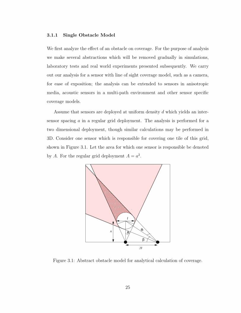
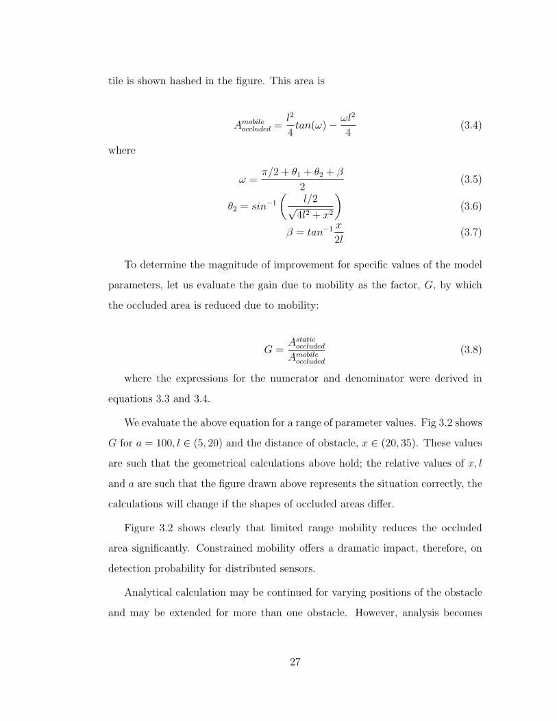
3.1.1 Single Obstacle Model
We first analyze the effect of an obstacle on coverage. For the purpose of analysis
we make several abstractions which will be removed gradually in simulations,
laboratory tests and real world experiments presented subsequently. We carry
out our analysis for a sensor with line of sight coverage model, such as a camera,
for ease of exposition; the analysis can be extended to sensors in anisotropic
media, acoustic sensors in a multi-path environment and other sensor specific
coverage models.
Assume that sensors are deployed at uniform density d which yields an inter-
sensor spacing a in a regular grid deployment. The analysis is performed for a
two dimensional deployment, though similar calculations may be performed in
3D. Consider one sensor which is responsible for covering one tile of this grid,
shown in Figure 3.1. Let the area for which one sensor is responsible be denoted
by A. For the regular grid deployment A = a2.
����������������������������������������������������������������������������������������������������������������������������������������������������������������������������������������
����������������������������������������������������������������������������������������������������������������������������������������������������������������������������������������
2l
l
β
x θ1θ2
Figure 3.1: Abstract obstacle model for analytical calculation of coverage.
25
Consider a circular obstacle of diameter l present in this tile which blocks
the coverage of the sensor. We will assume that the sensor is capable of limited
mobility over a range which is a small multiple of l.
Suppose the area occluded by the obstacle is Aoccluded (shown shaded in Figure
3.1). To quantify the coverage, we define the probability of mis-detection, PoM ,
as
PoM =1
A
∫
Aoccluded
ftarget(x, y)dxdy (3.1)
where ftarget(., .) is the probability density of the target location within A.
When there is no design time knowledge of the target location, ftarget(., .)
becomes a uniform probability density. For this case, PoM = Aoccluded/A.
When no obstacle is present, A is completely covered by the sensor and hence
PoM = 0. Now consider the case when one obstacle is present. Consider the
position of the obstacle shown in Fig. 3.1 such that both the tangents from the
sensor to the obstacle circle meet the top edge of the tile. Let θ1 be the angle
made by the tangent to the obstacle edge with the vertical line joining the sensor
and the center of the obstacle. Let the distance of the obstacle center from the
sensor be x. Then,
A = a2 − π
(
l
2
)2
(3.2)
Astaticoccluded = a2tanθ1 −
l2
4tanθ1
− (π + θ1)l2
8(3.3)
where θ = sin−1(l/2x). Next consider the case where the sensor is capable of
moving a small multiple of l, say 2l, on a track along the edge of the tile. The
occluded area when the camera may use any location along its track to cover the
26
tile is shown hashed in the figure. This area is
Amobileoccluded =
l2
4tan(ω)− ωl2
4(3.4)
where
ω =π/2 + θ1 + θ2 + β
2(3.5)
θ2 = sin−1
(
l/2√4l2 + x2
)
(3.6)
β = tan−1 x
2l(3.7)
To determine the magnitude of improvement for specific values of the model
parameters, let us evaluate the gain due to mobility as the factor, G, by which
the occluded area is reduced due to mobility:
G =Astatic
occluded
Amobileoccluded
(3.8)
where the expressions for the numerator and denominator were derived in
equations 3.3 and 3.4.
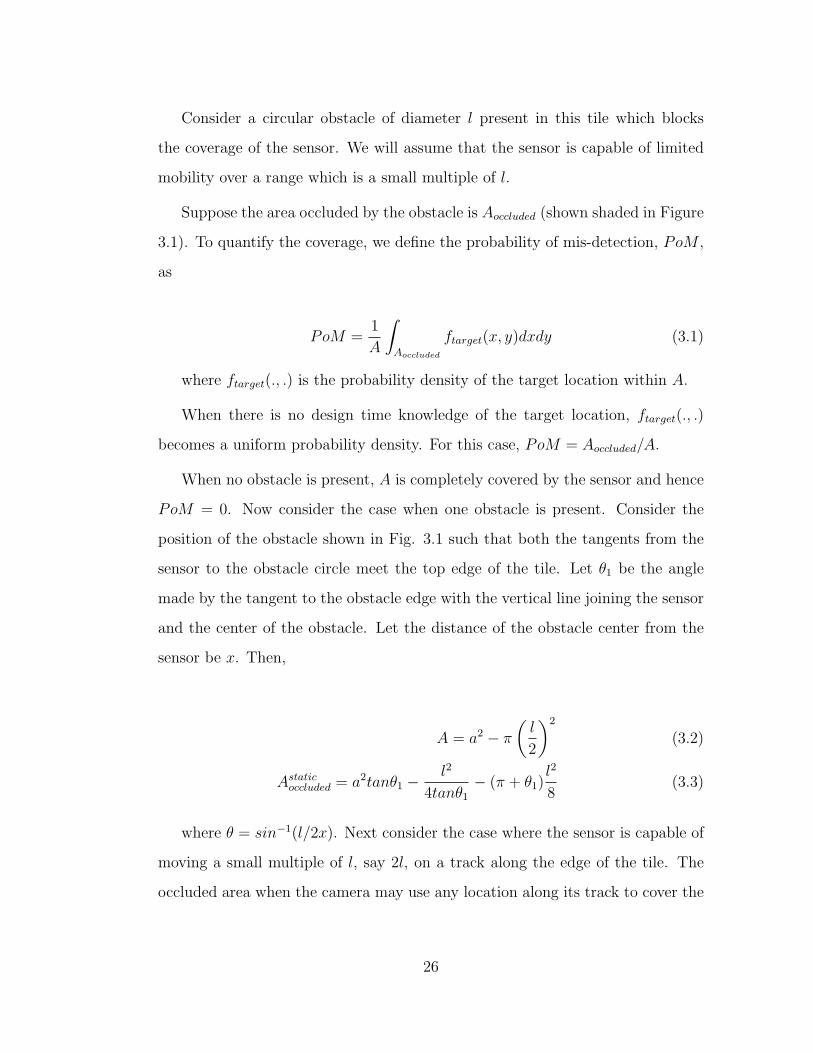
We evaluate the above equation for a range of parameter values. Fig 3.2 shows
G for a = 100, l ∈ (5, 20) and the distance of obstacle, x ∈ (20, 35). These values
are such that the geometrical calculations above hold; the relative values of x, l
and a are such that the figure drawn above represents the situation correctly, the
calculations will change if the shapes of occluded areas differ.
Figure 3.2 shows clearly that limited range mobility reduces the occluded
area significantly. Constrained mobility offers a dramatic impact, therefore, on
detection probability for distributed sensors.
Analytical calculation may be continued for varying positions of the obstacle
and may be extended for more than one obstacle. However, analysis becomes
27

20 25 30 35500
1000
1500
2000
2500
3000
Obstacle distance, x (m)
Red
uctio
n in
occ
lude
d ar
ea, G
(%
)
l=5l=10l=15l=20
Figure 3.2: Calculating the advantage due to mobility for a simplified obstacle
model.
intractable as the number of obstacles grows and we resort to simulations for
evaluating more complex and representative environments.
3.1.2 Multiple Obstacles
The simulations consider several scenarios with multiple obstacles. The simu-
lations model a 2D deployment; the effect of height is not accounted for in the
obstacle model. Three dimensional calculations would be needed when sensors
are observing the environment from a UAV or very high altitude.
Again, we consider sensors placed along edges of a square region, which as
before models one tile of a large deployment. The mobile sensor is assumed to
be able to move a short distance along the edge.
To model realistic obstacles, we first note than most everyday objects have
a small aspect ratio. Also, for the line of sight sensor, it is not the exact shape
28
of the obstacle but the angle subtended by it at the sensor which determines the
occlusion. With this reasoning, we simulate the obstacles as circular. A notable
exception to small aspect ratio objects are walls and other forms of boundaries
which will severely limit the coverage of a sensor and we do not expect small
motion to overcome the effect of walls.
The obstacle diameter is assumed to be a random variable with uniform dis-
tribution, between 0 and 2lav. The density of obstacles is represented as number
of obstacles per unit area. The obstacles are placed uniformly randomly over a
square area of size 100× 100. The random coordinates may lead to overlapping
obstacles causing the formation of complex obstacle shapes. As discussed before,
we are not concerned with the exact shape of an obstacle but rather with the
occlusion caused by it. The sensor is again assumed to be capable of moving a
distance dmove which is a small multiple of lav.
Coverage is measured by evaluating the area which is visible to the sensor
compared to the free area left in the square after the area occupied by the obsta-
cles themselves is subtracted. The line of sight from the sensor to every point in
the free area is tested and if there is an obstacle blocking it that point is assumed
occluded. Coverage can be calculated by counting the occluded points and the
visible points.
To suppress the effect of peculiar chance placements, for each choice of para-
meter values we average our measurements over 20 runs of the simulation. One
of the sample obstacle placements is shown in Figure 3.3, with one sensor placed
along the lower edge.
For the first simulation, there is one sensor placed at the center of the lower
edge. The value of lav is 5m. The obstacle density is varied from 1 obstacles in the
square region to 15 obstacles. Coverage is evaluated for three cases: when there
29

0 20 40 60 80 1000
10
20
30
40
50
60
70
80
90
100
Figure 3.3: Sample obstacles in deployment terrain (The small line along the
lower edge shows the track on which the sensor moves).
is no mobility, when the sensor can move lav to one side of the center position
and when the sensor can move 2lav, equally divided on both sides of the center
position. Figure 3.4 shows the fraction of free area covered in each case. For each
obstacle density, coverage is obtained by averaging over 20 obstacle placements,
in each of the three sensor mobility cases.
The gains due to mobility in varying obstacle density, compared to a static
sensor are shown in Figure 3.5. The gain is defined as:
G =PoMstatic
PoMmobile
(3.9)
The figure shows 200% to 700% gain for sensors with small mobility compared
to static sensors.
The next simulation studies the advantage due to mobility in varying obstacle
size. The value of lav varies between 5 and 20m in a 100× 100 area. The number
of obstacles is kept fixed at 10. Figure 3.6 shows the multiplicative reduction in
mis-detection probability, G. The labels 1 and 2 along the x-axis refer to cases
30

0 2 4 6 8 10 12 14 160.6
0.65
0.7
0.75
0.8
0.85
0.9
0.95
1
Number of Obstacles
Cov
erag
e Fr
actio
n (a
nd v
aria
nce
amon
g 20
runs
)
dmove
=0d
move = l
avd
move = 2l
av
Figure 3.4: Coverage with varying obstacle density, with and without mobility.
The error bars show the variance among 20 runs with different random obstacle
placements.
when the sensor is allowed to move lav and 2lav respectively. Again, actuation
shows significant advantage, giving more than a factor of 2 improvement. The
variance in the results from the 20 random topologies, not plotted for brevity, is
less than 0.05 in all cases. The simulation results are very encouraging and verify
that the performance gains expected in simplified analysis with a single obstacle
are also expected with realistic scenarios having multiple obstacles and varying
camera mobility range. These results motivate us to implement experimental
systems which utilize small motion capability.
3.1.3 Experiments
The experimental system studies the improvement in coverage in the presence
of realistic effects such as the actual detection algorithms operating on real sen-
sor data, in the presence of transducer noise. The sensor angle of view may be
constrained and illumination conditions may affect detection. Previous work on
31

0 2 4 6 8 10 12 14 160
100
200
300
400
500
600
700
800
Number of Obstacles
Per
cent
age
gain
due
to m
obili
ty
dmove
=lav
dmove
=2lav
Figure 3.5: Actuation advantage (multiplicative reduction in probability of mis-
-detection) in varying obstacle density.
coverage in sensor networks [WXZ03b, MKP01, LWF03] has been based only
on abstract sensor models, such as a circular disc coverage model, and not on
measurements with real sensors; our experiment is one of the first attempts to
corroborate the proposed coverage enhancement methods with real-world mea-
surements.
This section describes the camera test-bed built for this purpose and our
experiments on it in two different scenarios - a controlled laboratory environment
and an outdoor environment with trees and foliage.
32

1
2
5
10
15
20
0
100
200
300
400
500
600
dmove
/lav
lav
Perc
enta
ge g
ain
due
to m
obilit
y
Figure 3.6: Actuation advantage (multiplicative reduction in probability of mis-
-detection) with varying obstacle size.
3.1.3.1 Laboratory Test-bed with Cameras and Obstacles
Figure 3.7 shows a picture of obstacles in our laboratory test-bed, seen from the
camera location.
The sensor used on the test-bed is an Axis 2100 camera system [AXI]. The
camera system is equipped with rotational articulation to enable imaging in the
entire plane of rotation. The object being detected was large enough to cover
a detectable area in the captured image, even when placed at the maximum
distance from the camera in the region being covered.
The coordinates for obstacle placement are obtained from the actual location
of trees in the Wind River forest [Win03]. The size of tree stems is assumed equal
for simplicity of construction. Actual tree coordinates do not follow a uniformly
random distribution due to physiological phenomena and using actual forest tree
coordinates is expected to provide a realistic obstacle scenario. The obstacles
used here are cylinders with diameter of 1 foot. They are placed in a 12 foot by
33

TARGET
Figure 3.7: The laboratory test-bed for testing coverage advantage due to mobil-
ity.
12 foot grid. The tree coordinates are shown in Figure 3.8.
0 2 4 6 8 10 121
2
3
4
5
6
7
8
9
10
11
12
Figure 3.8: The coordinates of trees from Wind River forest [Win03] used to
place the obstacles in laboratory test-bed.
The target being detected is a small cylinder of a different color than the
obstacles. A simple image processing technique is used to detect the target in
34

the captured image. As the lighting in the laboratory is controlled, we can take
an image of the background with no target present and detect the target by
subtracting an image taken when the target is present from the background image.
If the target is completely occluded, it is will not be detected. If it is partially
occluded, we assume it as detected if the number of pixels visible is above a
certain threshold. This threshold procedure reduces the contribution of noise
associated with the camera system by ensuring that a minimum portion of the
target is observed in order to declare a positive detection.
The experiment is performed as follows. First the camera is placed at the
midpoint of one edge of the square area. With the camera stationary, the target
is moved to uniformly spaced locations on the 12′ × 12′ grid. The number of
locations at which the camera is able to detect the target divided by the total
number of locations at which the target was placed gives the coverage achieved
by the static sensor.
Next the camera is assumed to be able to move a distance of two feet. Cov-
erage is again computed using the previous target placement procedure but now
if the target can be detected by the camera by moving along its track, the target
is assumed detected.
Further, we vary the number of cameras available. One additional camera is
successively added on each of the other edges. The mis-detection probabilities
are plotted in Figure 3.9 for varying number of cameras, both for the stationary
case and the mobile case. The mis-detection with mobility is significantly lower
than the static case, reaching an order of magnitude improvement in some cases.
35

1 1.5 2 2.5 3 3.5 4
10−1
100
Number of Cameras
Pro
babi
lity
of M
is−d
etec
tion
(PoM
)
Mobile caseStatic case
Figure 3.9: Probability of Mis-detection in laboratory test-bed experiments: vary-
ing number of cameras. PoM is lower with mobility.
3.1.3.2 Experiment in Trees and Foliage
We also test our findings outside the laboratory, using a more realistic setting.
An environment with trees and foliage is selected, near our campus, shown in
Figure 3.10.
The obstacles are no longer ideal cylinders and cameras do not operate in
controlled lighting conditions. The cameras being used are not designed for out-
door usage and the image quality is affected by exposure to sunshine for the long
duration required for collecting data in our experiments. This leads to some er-
rors in our simple image processing techniques for detecting the target. It may
be noted that the foliage causes rather large occlusions and our mobility here is
much less than the mean obstacle diameter, instead of being an integral multiple
of it.
The experiment performed consists of one camera placed along one edge.
36

TARGET
Figure 3.10: Image of real world scene showing obstacles consisting of trees and
foliage, among which the target is to be detected.
Coverage is measured over a 12′ × 12′ grid in the forest. Detection probability is
first measured when the camera is fixed at the midpoint of the edge. Then the
camera is allowed to move two feet in one direction. Third the camera is allowed
to move 2 feet in both directions. The mis-detection probabilities and gains are
tabulated in Table 3.1. The measurements show that mobility even when lower
than average obstacle length is able to provide significant advantage in reducing
the uncertainty of sensing.
Table 3.1: Mis-detection probabilities with and without motion for real-world
experiment
CameraMode PoM G (%)(relative to static case)
STATIC 0.3885 -
MOVE, 1 direction 0.2374 163.65
MOVE, 2 directions 0.1942 200.05
37

3.1.4 Two-dimensional Motion on Infrastructure
We mention an example where constrained motion helps increase the resolution
of sensing, using a system that allows infrastructure supported motion in a two-
dimensional plane. We proposed a system that allows the motors and power
connections to be present at only one corner of the two dimensional plane being
covered. The cables themselves are used to move the node across the plane and
supply power to it. This reduces the payload moved by the motors since the
motors and power supplies do not have to be moved. The system is rapidly
deployable since it only requires the two supporting end poles to be installed at
the location of interest. A schematic of the system is shown in Figure 3.11.
Motor 1
Motor 2
Sensor
Plane of Motion
Figure 3.11: NIMS-LS: a system to provide infrastructure supported 2D motion.
Another system to provide 2D infrastructure supported motion was designed
in [HAG06]. The infrastructure consists of a cable suspended horizontally be-
tween two supports at opposite ends of the plane of motion. The horizontal
cable supports motion along the horizontal axis. A second cable in the vertical
direction is used for motion along the vertical axis.
38

Consider an application where the concentration of nitrate radical (NO−
3 ) is to
be mapped across the cross-section of a river, such as shown in Figure 3.12. The
River Width (m)
Riv
er D
epth
(m
)
0 5 10 15 20 25 30 350
0.2
0.4
0.6
0.8
1
Figure 3.12: Nitrate concentration (mg/l) across the cross-section of a river.
available nitrate sensor node has a transducer surface 0.1m × 0.1m that is used
for sensing. Suppose nitrate concentration is to be mapped at 0.5m resolution.
Then, installing the available sensor at every 0.5m across the river cross-section
along with the deployment infrastructure such as metal trusses to support the
sensors in the river is likely to interfere with the nitrate concentration map.
On the other hand, a sensor with constrained motion in a 2D plane across the
river cross-section, such as described above, can map the nitrate concentration
at the required resolution without interfering significantly with the phenomenon.
Assuming the concentration map does not change within the time it takes for the
sensor movement to be completed, the nitrate concentration can be mapped at
the required resolution.
3.2 Pan, Tilt, and Zoom Motion for Cameras
Pan, tilt and zoom can significantly extend the sensing coverage, despite its sim-
plicity and ease of practical realization. For instance, the area covered by a
camera can be increased by panning and tilting the camera head. As a represen-
39
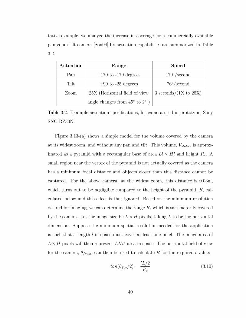
tative example, we analyze the increase in coverage for a commercially available
pan-zoom-tilt camera [Son04].Its actuation capabilities are summarized in Table
3.2.
Actuation Range Speed
Pan +170 to -170 degrees 170◦/second
Tilt +90 to -25 degrees 76◦/second
Zoom 25X (Horizontal field of view 3 seconds/(1X to 25X)
angle changes from 45◦ to 2◦ )
Table 3.2: Example actuation specifications, for camera used in prototype, Sony
SNC RZ30N.
Figure 3.13-(a) shows a simple model for the volume covered by the camera
at its widest zoom, and without any pan and tilt. This volume, Vstatic, is approx-
imated as a pyramid with a rectangular base of area Ll ×Hl and height Rs. A
small region near the vertex of the pyramid is not actually covered as the camera
has a minimum focal distance and objects closer than this distance cannot be
captured. For the above camera, at the widest zoom, this distance is 0.03m,
which turns out to be negligible compared to the height of the pyramid, R, cal-
culated below and this effect is thus ignored. Based on the minimum resolution
desired for imaging, we can determine the range Rs which is satisfactorily covered
by the camera. Let the image size be L×H pixels, taking L to be the horizontal
dimension. Suppose the minimum spatial resolution needed for the application
is such that a length l in space must cover at least one pixel. The image area of
L×H pixels will then represent LHl2 area in space. The horizontal field of view
for the camera, θfov,h, can then be used to calculate R for the required l value:
tan(θfov/2) =lL/2
Rs
(3.10)
40

R
L
H
(a) Covered Volume Model
Tilt
θtilt −θ
θtilt+
(b) Tilt Motility
Zoom
Pan
(c) Pan and Zoom Motility
Pan
Tilt
Zoom
(d) PZT Motility
Figure 3.13: Actuation in a PZT camera (a) volume covered without actuation
can be modeled as pyramid, (b) tilt capability increases the effective volume
covered, (c) combined pan and zoom capabilities further increase the volume
covered, and (d) volume covered when pan, tilt, and zoom are combined: this
can be viewed as a portion of a sphere swept out using pan and tilt, where the
thickness of the sphere depends on the zoom range.
The value of l depends on phenomenon size and the minimum image resolution
needed by detection algorithms. Suppose l = 1cm is used. For the sample camera,
θfov,h = 45◦, L = 640 pixels and H = 480 pixels, which yields Rs = 7.27m. This
41

value is within the focal range of the camera. The focal range may limit R and
hence the usable range of l. We also assume that the illumination is sufficient for
the zoom range available on the camera. Thus, Vstatic is given by:
Vstatic =LHRsl
2
3(3.11)
Now consider the volume covered with motility. When motorized zoom with a
zoom factor of z is used, the range covered becomes zRs. The additional volume
covered is a cuboid of depth (z−1)Rs and area Ll×Hl. The total volume covered
with zoom, Vz, becomes:
Vz = Vstatic + LH(z − 1)Rsl2 (3.12)
and corresponding gain factor due to zoom motility, gz, is gz = Vz/Vstatic = 3z−2.
Let the tilt angles with respect to the plane of pan rotation be denoted θ−tilt in
the downward direction and θ+tilt upwards, with their total being θtilt. The volume
covered when the tilt capability is used, Vt, can be viewed as the volume of a
sector of a disk of radius Rs, thickness Ll, and sector angle θtilt minus the volume
of two cone sectors of radius Rs, height Ll/2 and sector angle θtilt. This volume
is shown in Figure 3.13-(b). A half of the pyramid extends beyond the tilt range
on each side, and these additional edge volume segments extending beyond the
sector total up to Vs. The total volume covered with tilt motility, Vt, is thus:
Vt = Vstatic +θtilt
2π
[
πR2sLl − 2
(
1
3πR2
s
Ll
2
)]
(3.13)
The calculation of the volume covered using pan motility is very similar, and
is omitted for brevity. Figure 3.13-(c),(d) show the volumes covered when two or
more actuation modes are combined. Evaluating these volumes yields the overall
gain due to pan, zoom and tilt combined, gpzt, to be:
gpzt = (3z − 2) +θtiltRs
2Hl(3z2 + 1) +
42
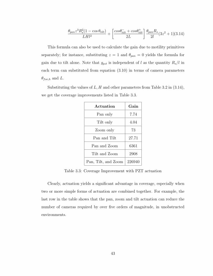
θpanz3R2
s(1− cos θtilt)
LHl2+
[
cosθ−tilt + cosθ+tilt
2L
]
θpanRs
2l(3z2 + 1)(3.14)
This formula can also be used to calculate the gain due to motility primitives
separately; for instance, substituting z = 1 and θpan = 0 yields the formula for
gain due to tilt alone. Note that gpzt is independent of l as the quantity Rs/l in
each term can substituted from equation (3.10) in terms of camera parameters
θfov,h and L.
Substituting the values of L,H and other parameters from Table 3.2 in (3.14),
we get the coverage improvements listed in Table 3.3.
Actuation Gain
Pan only 7.74
Tilt only 4.04
Zoom only 73
Pan and Tilt 27.71
Pan and Zoom 6361
Tilt and Zoom 2908
Pan, Tilt, and Zoom 226940
Table 3.3: Coverage Improvement with PZT actuation
Clearly, actuation yields a significant advantage in coverage, especially when
two or more simple forms of actuation are combined together. For example, the
last row in the table shows that the pan, zoom and tilt actuation can reduce the
number of cameras required by over five orders of magnitude, in unobstructed
environments.
43

3.2.1 Usable Range of PZT Motion
The above calculations assumed the entire range of motion capabilities is usable.
However, in a practical setting, only a part of it may be used, such as due to
the tolerable delay available for motion, or the motion triggering mechanism.
Suppose the motion triggering mechanism is such that the camera uses its pan,
tilt, and zoom motion to zoom in to a location where an event is detected from
its wide angle view. Then clearly, the entire pan range may not be utilized but
only the pan range equal to the field of view angle in the horizontal direction may
be used. Also, the useful zoom range is limited to the difference in resolutions
required for detection and the final sensing task. We analyze the coverage gain
with these effects next. Suppose the resolution required for the final sensing
objective is such that the camera can image up to the maximum distances Rs.
The volume covered by the camera can be modeled as a pyramid of height Rs
with the base area Lls × Hls, and its vertex at the camera1. This yields the
volume over which the desired sensing resolution is provided, say, Vs. Suppose
detection can occur when a distance ld is mapped to a single pixel-length, which
similarly leads to a volume Vd over which detection is feasible.
Figure 3.14-(a) shows the volumes Vs and Vd. The camera can provide the
resolution ls at points outside Vs, but within Vd, by using its pan, tilt and zoom
motion. The maximum advantage that may occur in coverage due to motion
is G = Vd/Vs, if the camera has motion capabilities to reach any point in Vd
at the resolution ls and sufficient time is available for that motion to occur.
Figure 3.14-(a) also shows the pan, tilt and zoom ranges required to cover the
entire Vd. Suppose the time taken for that motion, referred to as the actuation
delay, is τ . The advantage G may be reduced if the tolerable actuation delay
1A small region near the vertex may be too close for focus limitations but its volume isassumed insignificant compared to the entire pyramid
44

does not permit reaching some fraction of Vd. The tolerable delay τ depends on
the event dynamics. Consider again the example camera: it has a field of view
θfov,h = 45◦ in the horizontal direction and θfov,v = 30◦ in the vertical direction,
which determine the horizontal and vertical vertex angles respectively for Vd.
It has pan and tilt ranges of 340◦ and 115◦ respectively, which are more than
sufficient to cover the entire Vd. The zoom range is 25, which means that the
maximum ratio Rd/Rs supported is 25. The pan and tilt speeds are 170◦s−1 and
57.5◦s−1 respectively. The time taken for zoom is non-linear and was measured
experimentally for the entire zoom range (Figure 3.14-(b)).
dV
V
tilt
pan zooms
(a) Covered Volumes
0 5 10 15 20 25 300.5
1
1.5
2
2.5
Zoom Factor
Tim
e to
Mov
e fr
om Z
oom
1 (
s)
(b) Zoom Delay
Figure 3.14: (a) Covered volumes for detection and sensing phases, with the
pan, tilt, and zoom required to provide sensing resolution within the detection
volume. (b) The time to change zoom measured as a function of the zoom
step. The communication delay in sending the zoom command was separately
characterized and has been subtracted from the motion time.
The detailed calculation of the advantage in covered volume due to motion,
G, for these capabilities is skipped for brevity. The derived value of G is plotted
in Figure 3.15 for various values of τ ranging from zero to the maximum time
required to exploit the entire motion range and various values of Rd/Rs within
the zoom range of the camera. Note that G is quite large and hence plotted
45

on a log scale. The region in the figure corresponding to actuation delay above
1s and the ratio Rs/Rd > 2 shows more than an order of magnitude advantage
in coverage. Applications with sensing requirements that lie in this region will
benefit significantly from the algorithms discussed in this thesis.
00.5
11.5
22.5
0
10
20
300
1
2
3
4
5
Actuation Delay (s)R
det/R
sense
log 10
(G)
Figure 3.15: Evaluating coverage gain due to motion with varying actuation delay
and difference in detection and identification resolution.
3.2.2 Advantage with Multiple Nodes
The preceding analysis showed how motion can help improve sensing when it
is used for providing high resolution coverage on demand from a given pose.
There are additional ways in which motion may improve coverage, specifically by
optimizing the initial configuration itself. These additional advantages becomes
relevant when the sensor nodes with pan, tilt, and zoom capabilities are used in
a network, rather than at a single node.
First, a random deployment may cause two sensors to be covering overlapping
areas while other areas remain uncovered. Motion allows efficient orientation of
46

the sensors to cover non-overlapping areas.
Second, regions blocked by obstacles for one sensor may be viewable by
another sensor, if that sensor chooses the appropriate position or orientation.
Among the multiple possible network configurations, the positions of the nodes
can be collaboratively adjusted to minimize occlusions. Just as with infrastruc-
ture supported motion, pan, tilt, and zoom motion may also be used to achieve
this.
As an illustration, figure 3.16-(a) shows a random placement of 20 sensors
in a 25m × 25m area, each oriented randomly, and in the presence of obstacles.
The circles represent obstacles in the sensing medium and the sensor locations
are marked with small diamonds. The sectors of circles indicate covered regions,
0 10 200
5
10
15
20
25
0 10 200
5
10
15
20
25
(a) (b)
Figure 3.16: Instantaneous coverage increase: (a) a sample topology showing ran-
domly oriented sensors, and (b) sensor orientations changed using pan capability.
modeling a 45◦ field of view and a range, Rs = 7.3m, as calculated earlier for
the sample sensor. If these sensors have pan capability, their orientations can be
changed. Figure 3.16-(b) shows a changed network, where the number and loca-
47
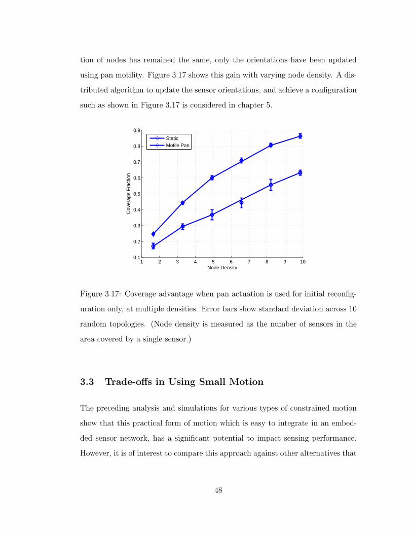
tion of nodes has remained the same, only the orientations have been updated
using pan motility. Figure 3.17 shows this gain with varying node density. A dis-
tributed algorithm to update the sensor orientations, and achieve a configuration
such as shown in Figure 3.17 is considered in chapter 5.
1 2 3 4 5 6 7 8 9 100.1
0.2
0.3
0.4
0.5
0.6
0.7
0.8
0.9
Node Density
Cov
erag
e F
ract
ion
StaticMotile Pan
Figure 3.17: Coverage advantage when pan actuation is used for initial reconfig-
uration only, at multiple densities. Error bars show standard deviation across 10
random topologies. (Node density is measured as the number of sensors in the
area covered by a single sensor.)
3.3 Trade-offs in Using Small Motion
The preceding analysis and simulations for various types of constrained motion
show that this practical form of motion which is easy to integrate in an embed-
ded sensor network, has a significant potential to impact sensing performance.
However, it is of interest to compare this approach against other alternatives that
48

may be used to improve sensing performance, and explore the trade-offs related
to various choices. There are two obvious alternatives to the use of motility.
One is to use a much higher density of static nodes and the other is to use an
even lower density of mobile nodes with long range motion capabilities. We will
discuss how small mobility compares to these.
3.3.1 Feasible Resolution
The deployment environment may limit the density of static sensors that may
be deployed. This limit may arise from various reasons. The ability to provide
mounting supports may be restricted to a limited number of locations within
the environment being monitored. The size of the sensor node limits the density
of deployment. A very high density of sensors may interfere with the phenom-
enon itself. Additionally network capacity, such as the channel bandwidth in a
wireless system, may limit the density of nodes. The provision for energy may
impose another limitation. If a wired energy infrastructure is provided, the den-
sity at which the cabling can be installed will limit the node density. For systems
using environmentally harvested energy, the amount of energy available in the
environment may limit the number of nodes.
Consider for instance the resolution feasible using a finite set of sensing re-
sources with and without motion. The image shown in Fig. 1.1(a) is obtained
using a 1 Megapixel (1MP) camera. The resolution of coverage over the region of
interest is: 40pixels/m at the near end of the road and 7pixels/m at the far end
of the road in the scene. In the image shown in Figure 1.1(c), the same 1MP sens-
ing resource is allocated to a small region achieving 200pixels/m resolution over
that region. Providing such high resolution coverage over the entire scene using
only static cameras, mounted at the same location, requires sensing resources of
49

784MP2.
Let us compare what motion may achieve. Suppose the 1MP camera used
to obtain the image is equipped with pan, tilt, and zoom motion capabilities.
Then, a zoom of 13X along with a small pan and tilt motion is sufficient for this
1MP camera to capture the image shown in Fig. 1.1(c) by focusing its sensing
resources selectively on a small region. These motion capabilities may be used
to get high resolution at any subregion of the scene shown in Fig. 1.1(a) and
thus motion has provided a virtual 784MP resolution using only 1MP sensing
resource. There are several issues in using the latter alternative such as the delay
in carrying out the pan, tilt, and zoom steps and the issue of finding out the
regions of interest. These issues will be discussed at length in the subsequent
sections. For situations when those issues can be satisfactorily addressed, using
motion is a significantly better alternative.
Thus, for the application scenario of interest, if the required resolution cannot
be achieved with a static system (such as if 784 1MP cameras are impractical to
be deployed in the above example), but can be achieved with a mobile network,
clearly, the use of motion is to be preferred.
There may be other applications where the resolution achieved by a static
network of low power cameras such as developed in [RBI05] may suffice. In some
instances, the area to be covered may be so small, such as a known choke point
in the field of view, that high resolution can be provided using a static cameras.
Again, motion may not be required to increase resolution in that scenario.
2Deploying cameras closer to the road could enable the use of much lower resolution camerassuch as used in red-light violation monitoring systems, but we assume that we are not allowedto install our equipment on the city road infrastructure.
50
3.3.2 System Deployment and Operation Cost
A second concern in choosing to use motion may be the system cost. Suppose the
number of nodes required in a static network is Ns and the number of mobile nodes
to get comparable coverage is Nm. Excluding certain applications such as those
where the sensor nodes are scattered from an airplane over an open field, most
applications, particularly those in indoor and urban environments, require each
sensor node to be individually deployed at a specific location, often manually. For
instance, deploying a camera requires mounting it on a wall or ceiling, installing
a dome or cover, and connecting it to a wired or wireless communication network.
For the current generation of cameras, deployment also involves providing a power
connection, although batteries or environmentally harvested energy may power
future generations of low power cameras. Suppose the deployment cost per node
is cdep. Suppose the cost of data processing at the back-end for data received from
a node is cp. These two costs are likely to be same for both static and mobile
nodes. Suppose also that the cost of a static node including maintenance for the
duration of deployment is cs. Denote the corresponding number for a mobile node
as cm. This number depends on the type of motion capabilities included in the
mobile node. The total system cost for the static case becomes Ns(cs + cdep + cp)
and that for the mobile case becomes Nm(cm + cdep + cp). Noting that the node
costs cs and cm are likely to diminish with advances in camera sensors and MEMS
based motion technology, in addition to the fact that cdep and cp are same for
both types of nodes, leads to the conclusion that the trade-off will be determined
primarily by values of Ns and Nm. For the current generation cameras, since the
difference between cs and cm is within an order of magnitude while the difference
between Ns and Nm is greater than an order of magnitude, typically several
orders of magnitude for examples considered in this thesis, again the trade-off is
51

dominated by Ns and Nm.
3.3.2.1 Example
We now consider an example coverage scenario and compare the Ns and Nm for
it. To decouple the trade-off arising due to motion delay for this example, let
us first assume that the persistence time or the Nyquist interval of the sensed
phenomenon is T = 3s, which allows the pan and linear motion motility to be
used fully. For nodes with unconstrained mobility, while the range of motion is
potentially infinite, only a finite motion is possible within the tolerable delay.
We assume a velocity v = 100cm/s for such mobile nodes, as navigation and
traction support for such speeds has already been demonstrated in experimental
platforms. We also allow the mobile nodes to be able to turn with maximum
agility at the same speed, which implies that an unconstrained mobile node may
move and orient to any position within the distance vT .
The exact relation between the numbers of static and mobile sensors required
is dependent on the medium and the nature of deployment, and hence we gen-
erate random topologies with multiple obstacle and sensor configurations. The
obstacles are again cylindrical and the sensors are arranged in a 2D deployment
interspersed with the obstacles, over a 20m× 20m area. Ten random topologies
of obstacles and sensor placement are evaluated. The number of sensors is varied
to compare the coverage at different node densities. We evaluate the coverage
for four alternatives: static nodes, nodes with pan only motility, nodes with one
dimensional limited linear motility, and nodes with full unconstrained mobility.
Note that only a single calculation is performed for the fully mobile nodes, as
the initial random configuration is not relevant for this case; these nodes may
re-position themselves to the best initial configuration from which the allowable
52

mobility range of vT then allows them to cover the maximum area.
Figure 3.18 shows these results. Clearly, lower densities are required with
actuation for the same coverage quality. For instance, at 90% coverage, the
static density is 7 times higher than that with pan actuation. This suggests
small actuation can significantly lower the system cost. Unconstrained motion
has an even lower Nm but the cost and complexity of the mobile nodes may be
unacceptable for the system.
0.4 0.5 0.6 0.7 0.8 0.9 110
0
101
102
Coverage Fraction
Nod
e D
ensi
ty
Static NetworkLinear motionPan MotionFully Mobile
Figure 3.18: Alternative deployments: Coverage fraction with and without ac-
tuation at different deployment densities. Node density is the number of nodes
in a 20m × 20m square region, where each sensor covers a sector of 45◦ with
radius Rs = 7.3m. The error bars show the standard deviation across 10 random
topologies simulated.
Such numbers for Ns and Nm provide an approximate insight into the ap-
propriate system design choice, since the operational and deployment costs are
53

determined largely by these two quantities. One may however, for a specific sys-
tem, compute the node costs as well and compare the system cost in terms of the
node costs.
The cost needs be evaluated for the particular sensors of interest for a sys-
tem, and the costs may change over time. Here we compare the system cost
for known values of cs and cm for various motion alternatives. First, we do not
account for (cdep + cp), which makes the comparison harsher on the alternatives
with motion. Installation costs as high as 75% of the system cost have been
reported [Far01]. Here, the savings in (cdep + cp) due to a lower Nm compared to
a static system are not being considered. Second, the off-the-shelf fully mobile
nodes do not have built-in reliable navigation and localization subsystems, rather
they have a traction platform with appropriate interfaces for adding deployment
specific navigational support. We ignore the costs of these additions, thus losing
the significant advantage that motile nodes have in that they do not need such
extra support. Third, the cost of the motile node considered is with three motile
capabilities- pan, tilt, and zoom even though only the pan capability is considered
in the above density evaluation. Obviously, the cost of a pan-only camera will
be lower than one with all three motility primitives. Figure 3.19 shows the cost
trade-off, and even with the harsher comparison, the motile nodes offer a signif-
icant advantage. The costs considered are USD 800 for a static network camera
[SNC04], 1300 for a pan-tilt-zoom network camera from the same manufacturer
and having similar optical capabilities [Son04], and 35000 for a fully mobile node
[Pac04]. For linear actuation, we assumed the cost to be 1200, assuming the
static node cost plus an additional track, motor and motor controller.
54

1 2 3 40
20
40
60
80
100
120
Cos
t (th
ousa
nds)
Fully Mobile Static Linear Pan
Figure 3.19: Converting the node density to total network cost, at 90% coverage
point.
3.3.3 Actuation Delay
Another difference between a static and mobile network is that while in a static
network, the sensing is instantaneous, it is not so in a mobile one. Since the mobile
camera takes a finite non-zero time for the actuating to the region of interest,
there is a delay before the application receives the desired high-resolution data.
We call this delay the actuation delay. The advantage in resolution depends on
the tolerable actuation delay; the motion advantage disappears if the tolerable
delay is zero. Hence, this is a crucial issue in deciding whether motion may be
used.
The actuation delay scales better than linearly with the number of cameras
saved. Recall the earlier example where 784 static 1MP cameras were required
55

to obtain the desired resolution. A naıve approach can achieve a linear scaling
in delay. For instance, a single camera may be actuated to perform a raster
scan visiting the appropriate pan, tilt, and zoom poses to successively cover the
small regions covered by the 784 cameras. However, a better strategy such as
using the single 1MP camera to cover the entire scene at low resolution, applying
a low resolution algorithm to detect regions of interest in the field of view and
actuating only to cover those regions, reduces the delay significantly. In this case,
the camera does not visit all 784 poses but only a few of those, depending on the
number of detected events.
We will consider the delay trade-off in greater depth in designing the motion
coordination methods to exploit small motion capabilities for improving sensing
performance.
56

CHAPTER 4
System Architecture
The preceding discussion motivated the choice of small motion for improving
sensing performance in certain scenarios as opposed to other alternatives. In
scenarios where such motion is indeed the preferred choice, a key design issue is
to provide a system architecture that exploits motion capabilities effectively to
provide the best possible sensing performance. As mentioned before, we design
our methods for a system of cameras with pan, tilt, and zoom capabilities and
some of our design choices are thus specific to image sensors.
A naıve method to use motion for reducing the sensing uncertainty is to
successively allocate the available sensing resources to small regions such that high
quality coverage is provided at each region, in a time shared manner. However,
this method has a high delay penalty. An alternative method, that promises
significant advantages in delay, is feasible in several applications. This method
is as follows: allocate available sensing resources sparsely to cover the region
of interest at a low resolution that is sufficient to detect the phenomenon of
interest, and then selectively concentrate more sensing resources on regions where
the phenomenon is detected, providing an equivalent high-resolution coverage to
the overlying application using the sensor network. This approach is feasible
in all applications where a low resolution coverage is sufficient to detect the
phenomenon, such that high resolution coverage may then be provided only at
the locations where the phenomenon of interest is detected. There are several
57

applications where detection of an event of interest may be carried out at low
resolution. For instance faces can be detected using color detection [BSP04],
which requires a lower resolution than required for recognizing the faces. Humans
or vehicles in a scene may be detected using motion detection, whereas high
resolution coverage may be required for the actual surveillance application logging
a high resolution image of the visitors. In other applications, an alternate sensor
modality may be used for detection. For instance, magnetic sensors may be
used to detect vehicles and then image sensing resources may be allocated to
the required region. An acoustic beam forming technique may be used to detect
where an animal call originates [WEG03] for an ecology application, or where
a shooter is present for an urban security application [MSL04], and then high
resolution imaging may be directed toward that location.
Obviously, one of the system components required in realizing this approach
is a motion control method to carry out the motion required each time a phenom-
enon detection occurs. A simple example of this motion occurs in a camera with
pan, tilt and zoom capabilities: the camera may zoom in to the pixel location in
its field of view where a phenomenon of interest is detected. More sophisticated
motion strategies may be used for other objectives such as providing coverage
by multiple cameras when a phenomenon of interest is detected by one of them.
The exact requirements are application specific, and some methods have been
explored for such motion control [CDB04, CLF01, THM00, STE98].
Somewhat less obvious perhaps, and not previously studied to the best of our
knowledge, is the need for methods that allows the system to use the motion capa-
bilities effectively, such as with low delay, for the above mentioned motion control
component. We focus our attention on this latter aspect. Before the movement of
nodes to provide high resolution coverage takes place, the phenomenon must be
58

detected and the system is thus required to provide a good detection performance.
Further, when the movement occurs, the actuation delay is a key consideration,
particularly when the mobile network approach is compared to the alternative of
using a higher density of static sensors to achieve the same resolution. Clearly,
this delay should be characterized. The system should use motion capabilities
in such a way that the actuation delay is small for phenomena occurring at any
point in the area covered by the network. The limits on tolerable delay will also
limit the range of motion that may be used.
Our objective is to develop a system architecture that provides the required
detection performance and helps minimize the actuation delay.
Additionally, the system architecture should also attempt to exploit any infor-
mation available about the deployment environment. Specifically, the following
two types of information may be useful in controlling motion: a map of obstacles
in the sensing medium and the expected spatial distribution of the phenomenon
being sensed. It is desirable that the system architecture include components in
the system to learn such information and that it allows the network to gather
and use such information in a distributed manner.
We now discuss our system design in view of the design objectives mentioned
above and also describe additional design choices made in our system. We are
not concerned with the actual application level image processing algorithms but
only with providing the high resolution image for such processing.
The various system components required to support the above mentioned
objectives have been modularized into the blocks shown in Figure 4.1.
Block I, labeled medium characteristics, represents any means available to the
network for learning the locations of the obstacles. If available, this knowledge
helps the motion strategy to minimize occlusions. Such methods may be based
59
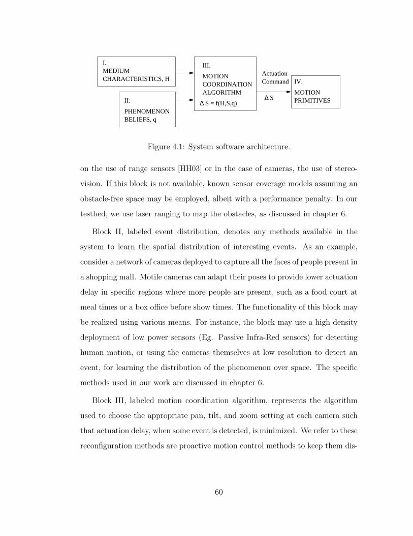
S = f(H,S,q)
I.MEDIUM CHARACTERISTICS, H
II.
PHENOMENONBELIEFS, q
III.
MOTIONPRIMITIVES
IV.MOTIONCOORDINATIONALGORITHM
CommandActuation
S∆∆
Figure 4.1: System software architecture.
on the use of range sensors [HH03] or in the case of cameras, the use of stereo-
vision. If this block is not available, known sensor coverage models assuming an
obstacle-free space may be employed, albeit with a performance penalty. In our
testbed, we use laser ranging to map the obstacles, as discussed in chapter 6.
Block II, labeled event distribution, denotes any methods available in the
system to learn the spatial distribution of interesting events. As an example,
consider a network of cameras deployed to capture all the faces of people present in
a shopping mall. Motile cameras can adapt their poses to provide lower actuation
delay in specific regions where more people are present, such as a food court at
meal times or a box office before show times. The functionality of this block may
be realized using various means. For instance, the block may use a high density
deployment of low power sensors (Eg. Passive Infra-Red sensors) for detecting
human motion, or using the cameras themselves at low resolution to detect an
event, for learning the distribution of the phenomenon over space. The specific
methods used in our work are discussed in chapter 6.
Block III, labeled motion coordination algorithm, represents the algorithm
used to choose the appropriate pan, tilt, and zoom setting at each camera such
that actuation delay, when some event is detected, is minimized. We refer to these
reconfiguration methods are proactive motion control methods to keep them dis-
60
tinct from the motion control methods used reactively after an event is detected,
for zooming in to that particular event and sensing it at high resolution. This
block also includes the network protocol required to implement the motion co-
ordination algorithm in a distributed manner. We discuss this block in greater
detail in chapter 5.
Block IV, labeled motion actuators, represents the motion capabilities avail-
able in the system. These motion capabilities are used both by the proactive
method to choose a good configuration for the network and by the reactive meth-
ods for providing the high resolution sensing when an interesting event is detected.
In our system these actuators are the pan, tilt, and zoom motors in the camera.
The camera used allows controlling its motion capabilities via sending it com-
mand packets in HTTP format with hardware specific values for various motion
settings. We developed a driver, in Java, with a programmer friendly interface
that accepts the required pan, tilt, and zoom motion steps in decimal values. Our
driver takes care of converting these to hardware specific format and packetizing
them as per the protocol required by the hardware.
This architecture is distinct from previously designed active camera networks
that used motion to patrol larger areas [CRZ04, CLF01, STE98, CDB04] that
required constant motion for the patrol. On the other hand, the low resolution
detection phase that we use does not require constant motion. Further those
methods are mostly designed for the reactive phase of tracking events after being
detected. That is distinct from the high-resolution objective we present. Also, the
previous works do not proactively configure the system to reduce the actuation
delay.
Assumption: In designing our system architecture in view of the above design
issues, we have made the following general assumption. We assume that each sen-
61
sor knows its location. This assumption is required only for improving the sensing
performance through coordination among multiple nodes. A local rudimentary
strategy to use motion without any coordination among sensors is also mentioned,
and while it does not require the use of location information, such a strategy per-
forms significantly worse than one with coordination. The assumption about the
availability of location information is reasonable in many applications since the
location information is required to geostamp the sensor data itself. Several lo-
calization strategies have been proposed for sensor networks [SHS01, MLR04] in
general and for networks of cameras in particular [DR04, FGP06]. For the type
of motion being considered in our work, even a deployment time record of node
installation locations suffices.
4.1 Technology Context
While our prototype is implemented using the current technology generation of
cameras, we believe that our system architecture is designed to support the antic-
ipated technology trends in this domain. More compact and lower power cameras
are becoming available for use in wireless sensor networks. MEMS based motion
technology will enable significantly more compact and lower power pan and tilt
mechanisms for such devices. Electrically controlled lens focus for changing the
zoom, such as being developed for zoom-capable cellphone cameras, will enable
the zoom capability to be accessible in compact low power wireless camera nodes
likely to be used in future sensor networks. As more and more applications that
use image data emerge given the increasing accessibility of the underlying tech-
nology, our methods for increasing the resolution will be increasingly relevant
for newer generations of camera networks. Further the potential for significantly
larger numbers of cameras made feasible through these emerging technologies will
62

directly benefit from the distributed and scalable nature of our methods.
Also, as technology evolves, the image resolution in terms of number of pixels
at a camera and the processing capabilities may increase, such as with Moore’s
Law. This may enable a given number of static cameras in a network to achieve a
higher resolution than possible with the current generation hardware. For certain
applications, this increased resolution may mean that the required resolution
becomes feasible with static cameras alone. The architecture we presented may
be used to obtain still higher resolution when it helps enable newer applications
or improve the performance of existing ones further.
63

CHAPTER 5
Motion Coordination Methods
We now consider block III of Figure 4.1 in detail: motion coordination algorithms
to achieve a desirable network configuration, and adapt it to the spatio-temporal
dynamics of the environment. Our focus is on distributed methods, due to scal-
ability concerns.
We express the problem of motion coordination algorithm design as an opti-
mization of a specific sensing performance objective. This performance objective
models the two key considerations in using motion - the actuation delay and the
detection activity required to guide the actuation. We begin with the discussion
of a quantitative metric to characterize this performance objective.
5.1 Sensing Performance
The first important consideration in motion coordination is the choice of the
sensing performance metric to quantify the value of a given network configuration.
Our camera coverage model depends on three parameters. The camera can view
any point not closer than its minimum focal distance Rmin, and not farther than
Rmax beyond which distance the spatial resolution is too poor to be of interest.
The camera has an angular field of view θfov. The three parameters Rmax, Rmin,
and θfov, change with the zoom setting of the camera. Given this model, the
sensing performance is characterized as follows.
64

5.1.1 Actuation Delay
The first quantity of interest is the actuation delay achieved by the network
configuration. As mentioned before, complete coverage is only provided at a
resolution lower than required for the final sensing application, and the cameras
are zoomed in to the relevant location when an event of interest is detected. The
actuation delay depends on the time taken by the camera to actuate (using its
pan, tilt, and zoom motion) for providing the required high resolution coverage
after an event is detected. It is defined concretely below.
Let the region to be covered by the network be denoted by A and let p be a
point in A. Suppose an event is detected at a point p. Suppose the time taken
by the camera to pan, tilt and zoom for focusing at the point p is denoted by
τ(p). It can be measured in terms of the motor capabilities of the node. Since
the pan and zoom are driven by separate motors and can occur in parallel, the
time required is:
τ(p) = max{δθp ∗ ωp, tp(δz)} (5.1)
where δθp is the pan angle to be moved to direct the sensor at p, ωp is the
angular pan speed, δz is the change in zoom required for achieving the required
classification resolution at p, and tp(δz) is the time required for changing the
zoom. Note that tp(δz) is a non-linear function of δz and a closed form expression
is not available for it. We have experimentally measured it for integral values
of δz for our sensor, and we use a linear interpolation in between the measured
values (Figure 3.14-(b)). The tilt time can be considered similarly as the pan
time, but our system deployment is two-dimensional and hence tilt is ignored.
This quantity τ(p) is defined to be the actuation delay for that particular
point p, for the given camera. In a network, multiple cameras may be able to
actuate to point p. We define τ(p) to be the one required by the specific camera
65
chosen for detection, as described below.
5.1.2 Detection Performance
Second, the coverage metric must also characterize the detection performance.
Several possible metrics exist for this, beginning with a purely geometric cov-
erage metric which quantifies the area in line of sight of the sensors, to more
sophisticated estimation theoretic metrics which quantify the probability of de-
tection based on the noise models and collaboration among sensors. Let c(p)
denote the detection performance at point p. Since detection depends on resolu-
tion, we model c(p) as proportional to the resolution at which a sensor s views p,
measured in the number of pixels per unit area. This is a more accurate model
than a purely distance based one, since the resolution depends not only on the
distance but also the zoom setting of the camera and obstacles in the medium.
For simplicity we assume no coordination among sensors for detection. Since
multiple cameras may have c(p) in their field of view, we define c(p) to be the
highest value provided by any one of sensors observing p.
5.1.3 Performance Objective
To aggregate the above factors into a single metric, we consider a linear com-
bination of the two metrics to determine the sensing performance, f(p), at a
point:
f(p) = w ∗ c(p) + (1− w){1/τ(p)} (5.2)
The choice of the weighting parameter w, where 0 ≤ w ≤ 1, determines the
proportion of the contribution of actuation delay and detection terms to the
performance. The value 1/τ(p) is capped to a maximum when τ(p) = 0.
66

Apart from maximizing the probability of detection, and minimizing the ac-
tuation delay, it may also be of interest to maximize the area covered. Let 1(p)
be a binary function which takes the value 1 at covered points and 0 at others.
The network may have to be geared toward regions where more events are
expected. Suppose that the event distribution function is known at all points
p ∈ A and is denoted q(p). Considering the above factors, we define the coverage
utility at a point as:
u(p) = (1− α)f(p) ∗ q(p) + α ∗ 1(p) (5.3)
where α is a constant weight, 0 ≤ α ≤ 1, determining the significance of coverage
alone. Note that the second term in the above equation is not multiplied by q(p).
This allows maximizing the area covered, even when events are concentrated in
a small region, by setting the value of α to be high. Methods to learn q(p) are
discussed in chapter 6.
Suppose the state, or pose, of a sensor node i is denoted by si = {θp, z},where θp and z represent the pan and zoom settings respectively. The network
configuration, for a network of N nodes is then denoted by S = {s1, s2, ..., sN}.Given the pan and zoom ranges of a node, the node state si lies in a set Si =
{[θminp , θmax
p ], [1, zmax]}, where the superscripts min and max represent the mini-
mum and maximum possible values respectively for the superscripted parameters.
Let S represent the resultant set of possible network configurations. It is given
by:
S = S1 × S2 × . . .× SN (5.4)
Using the metric defined above for each point, we now express the overall utility
of a network configuration, S, as:
U(S) =∑
p∈A
u(p) (5.5)
67

The network reconfiguration problem can now be expressed as an optimiza-
tion problem, where the goal is to determine the network configuration which
maximizes the coverage utility:
Sopt = maxS∈S
U(S) (5.6)
5.2 Distributed Motion Coordination
We now discuss a distributed algorithm to solve the above problem. A distributed
approach is advantageous due to the reasons discussed below.
5.2.1 Complexity Considerations
It is not immediately obvious how the optimization problem can be solved effi-
ciently because the optimization problem in (5.6) is NP-hard. Consider a special
case of the problem: α = 1. In this case the utility function is reduced to max-
imizing the coverage due to N sensors over a polygonal region with obstacles.
So, if the problem in (5.6) can be solved in polynomial time, then a polynomial
time solution exists to maximize coverage in a polygonal region with obstacles.
However, that problem is known to be NP hard [CN88]. Thus, the problem in
(5.6) is clearly NP-hard.
Further, the nature of c(p) and τ(p) implies that U(S) is not only non-linear
but also not known in a closed form – it can only be evaluated numerically for
each S. As seen from equation (5.4), the search space is exponential in N and a
brute force search over S is clearly out of the question.
The performance metric being used for optimization is a global metric for the
entire network and depends on the state of multiple sensors. The phenomenon
distribution and medium characteristics are learned locally. Thus, the perfor-
68
mance metric is not known at individual sensors given their local views and only
partial knowledge about q(p).
5.2.2 A Distributed Approach
A distributed solution will thus help ameliorate both communication overheads
and computational complexity. Here, we define an algorithm to be distributed, if
under its execution, each node exchanges messages only within a local neighbor-
hood rather than with a central coordination entity or the entire network. The
desirable local neighborhood for a node should minimize the number of commu-
nication hops required for coordination, and its size should not increase with the
network size N .
Consider the utility function U(S) defined in equation (5.5). This function is
inherently distributed in that the utility value at a point p can only be influenced
by a subset of the sensors: the ones which have p in their line of sight and within
the maximum range of view from one or more of their possible poses. Denote
the set of sensors which influence the utility value at p by β(p). Collect together
into a sub-region Bj, all those points which share the common influencing sensor
set β(p), and denote this sensor subset by βj. Suppose the entire region Acan be divided into K such sub-regions. By definition the {Bj}Kj=1 are disjoint
(the corresponding βj are not). There may be points in region A that are not
covered by any of the sensors; as a matter of notation, these may be denoted
by BK corresponding to βK = Φ, the null set. The utility function can now be
decomposed into a summation over these disjoint sub-regions:
U(S) =K
∑
j=1
∑
p∈Bj
u(p) (5.7)
Since each Bj corresponds to a sensor subset βj and a set of N sensors may
69

have 2N subsets, the number of terms in the above summation is potentially
exponential. We can however map the above decomposition to one where the
number of terms is linear in N . Let γi denote the subset of sensors which is the
union of all subsets βj to which sensor i belongs:
γi = {j|∃βk such that (i, j) ∈ βk} (5.8)
The utility in the region within range of sensor i can only be affected by the
sensors in γi. Given the state of each sensor in γi, sensor i can compute the set of
points Γi at which i gives the highest f(p) value. The sub-regions Γi are disjoint
(though the sensor subsets γi are not) and {Γi}Ni=1 ∪ BK = A. Hence the utility
function can be decomposed as:
U(S) =N
∑
i=1
∑
p∈Γi
u(p) (5.9)
The interesting property of this decomposition is that each each sensor only
needs to communicate with sensors in γi to determine U(S) over Γi. We call γi
the neighborhood of sensor i. The set γi includes all sensors which may affect
the computation of Γi from any pose selected at those sensors.
Suppose the region influenced by sensor i from all its poses is Vi. Then, the
set γi includes potentially all sensors influencing any point in Vi. The expected
cardinality of this set depends on the deployment density and the maximum
distance up to which a sensor may influence coverage. For most practical sensors,
the distance up to which they may sense is bounded, which implies that the
cardinality of γi stays constant even as the network size, N , increases, at a given
deployment density.
70

5.2.3 Coordination Algorithm
We now describe a distributed algorithm which requires each sensor to coordinate
only with sensors within γi and yet improve the global utility function. Suppose
a mechanism is available at sensor i to ensure that when it is changing its pose,
all other sensors in γi will remain static. The communication protocol to realize
this mechanism, and other implementation details will be discussed in the next
section. The algorithm then proceeds as follows.
Sensor i searches over all its possible pan settings, and chooses the one for
which the utility evaluated over Vi is maximum:
θp(i) = maxθp∈[θmin
p ,θmaxp ]
∑
p∈Vi
u(p) (5.10)
This is a one dimensional search and thus computationally tractable. After se-
lecting its best pan setting, the sensor similarly selects its best zoom setting.
After this pose update, sensor i stops and some other sensor j waiting on i may
update its pose, again making sure that sensors in γj stay static during its update
step.
This change in pose at i affects all Γj for j ∈ γi. However, it does not affect
sensors not in γj and they may be changing their poses in parallel with sensor
i using the same method. This property makes the algorithm distributed over
neighborhoods γi. The sensors update their poses in an arbitrary order.
5.2.3.1 Termination Condition
The termination condition in the protocol is chosen for ease of distributed imple-
mentation. In centralized optimizations, a stopping criterion that can determine
when to stop the iterations is to check when the change in the estimate of the
optima has become insignificant over the past few iterations. However, in the
71

distributed setting, the global utility metric is not available to any node. Even if
the parameters in control of a particular node are not changing from one iteration
to the next, the parameters at other nodes may be changing and determining the
stopping time would thus require global coordination. The distributed termina-
tion condition is that a node will assume its actuation has terminated when the
improvement increment in local utility is below a threshold ∆. In our implemen-
tation discussed in section 5.4, the value of ∆ is set to 0.1% of the previously
measured utility over Vi and may vary from sensor to sensor.
Note that a sensor need not physically carry out the actuation until it reaches
the termination condition of the algorithm. It only needs to communicate its
updated pose for the coordination mechanism to work.
5.2.3.2 Example
Before analyzing the convergence and other properties of interest, let us visualize
the above update procedure for a simple example with two sensors. Consider
a rectangular region with a few obstacles and two cameras placed at diagonally
opposite corners, as shown in Figure 5.1. Each camera can pan 90◦, in its corner.
To reduce the dimensionality of the search space to two for easier visualization, let
us ignore zoom. The utility function achieved for all combinations of pan angles
at each camera is shown in Fig. 5.2. The pose selection algorithm described
above proceeds as follows: sensor C1 first selects a pan, θp(1), which maximizes
the utility in its region of influence. This change is configuration is seen as line
segment A in Figure 5.2. Then, sensor C2 selects a pan pose, θp(2), for this given
value of θp(1), and line segment B shows the change in network configuration. In
the next iteration, again C1 selects a new pan θp(1) moving along line segment
C.
72

Figure 5.1: Illustrative scenario for motion coordination algorithm. The white
cirular regions are obstacles. The darker shade is uncovered region. The lighter
shaded regions represent covered areas, where lighter regions represent better
detection.
At each step, our algorithm searches along a line in the 2N -dimensional search
space, S, and so we will refer to the above optimization procedure as incremental
line search (ILS). The procedure is incremental at each node but not at the
network level. Multiple nodes may be actuating in parallel. The neighborhoods
γi may be overlapping implying the reconfiguration process cannot be broken
down as occuring in each neighborhood separately but the constraints within
each subset γi must be satisfied.
Note that in addition to the above method for configuring the network, an-
other motion control algorithm is also required to move the cameras after an
event is detected for providing the required high resolution coverage. For this
task, we use a simple method that zooms in to the pixel location in the image
73

0 20 40 60 80 100 0
50
100
2000
4000
6000
8000
10000
12000
14000
16000
θp(1)
θp(2)
U(S
)
A
B
C
Figure 5.2: Utility function for various possible pan pose combinations. The θp
values are in degrees, measured counter-clockwise from initial camera pose. The
utility function has multiple local maxima, even for this simple scenario.
where an event is detected. One advantage of this approach is that the spatial
location of the detected event is not required. More sophisticated methods which
may move multiple cameras in response to detected events have been studied in
other works [CDB04, CLF01, THM00, STE98].
5.3 Convergence and Other Properties of the Motion Co-
ordination Algorithm
While the proposed algorithm is not guaranteed to find the global optimum, it
has several desirable properties that are discussed below, including convergence
to a stable state.
74
An important property of the above optimization procedure is that it does
not require a closed form expression for the utility function, but may proceed
using only a numerical computation. It does not make any assumptions on the
smoothness or differentiability of the objective function. This makes the above
procedure amenable to several realistic performance metrics, in the presence of
non-linearities in actuation and the effect of obstacles.
Further, the termination condition used is distributed, and hence no global
coordination is required for the termination. A side effect of this is that no node
in the network may know when the actuation has terminated globally.
Another important property is the convergence of the network configuration
to a stable state. Even though the sensors may update their local poses without
any global coordination, the network utility function will not oscillate. Further,
the utility will reach a local maximum1, though not necessarily the global one,
which is hard to ensure without global coordination. We prove this convergence
property below.
Lemma 5.3.1 (Monotonicity of ILS) Under ILS execution, the global net-
work utility increases monotonically.
Proof: Assume first that only one sensor i in the entire network updates its pose
at a time. Suppose the network configuration after iteration t is denoted St. The
region A can be viewed as consisting of two disjoint subregions Vi, the region
influenced by sensor i from any of its poses, and A − Vi. The utility can be
expressed as:
U(St) =∑
p∈Vi
u(p) +∑
p∈A−Vi
u(p) (5.11)
1As seen in Figure 5.2, the maximum found by ILS is not necessarily the local maximumclosest to its starting point, unlike gradient descent based methods.
75

The update at sensor i does not affect the second term and it thus stays constant
at this iteration. The first term only depends on the region over which utility is
computed by i and since i choses a pose to maximize this term, this term can
only increase or stay constant. Thus when only one sensor updates at a given
iteration, monotonicity holds:
U(St+1) ≥ U(St) (5.12)
Now, suppose multiple sensors update in parallel. However, the coordination
over γi ensures that no sensor that affects Vi will update its pose when i is
moving. Thus, we can consider the region A − Vi independently. For another
moving sensor j, we can decompose A − Vi into two disjoint sets A − Vi − Vj
and Vj. An equation similar to (5.11) can then be written over these two sub-
regions. Recursively applying the same argument, all sensors j which update in
parallel within the coordination constraint over respective γj can only lead to a
monotonic increase in the global network utility regardless of update order. �
Theorem 5.3.1 (Convergence of ILS) The network configuration converges
to a stable state using ILS.
Proof: The proof follows from the fact that a monotonically increasing function
can either grow unbounded, or stabilize to a fixed value. Since the definition of
u(p) always yields a finite value and a summation over a finite region A ensures
that U cannot grow infinitely and hence the ILS algorithm will cause the network
configuration to converge to a stable state. Noting further that the actuation step
is lower bounded and can never be infinitesimally small, the convergence must
occur in a finite number of steps. �
As long as the decomposition in equation (5.5) holds, ILS can be used for
arbitrary performance metrics, other than the one discussed above. Generaliza-
76

tions include examples where the objective is not classification but tracking the
movement of events after detection. Instead of time τ(p), the metric of interest
would be the localization quality which might depend on the angle and distance
from the nearest two sensors for any point p.
5.3.1 Graceful Degradation
Note that the monotonicity is valid as long as other environmental parame-
ters such as the obstacles and phenomenon distribution remain stationary. The
monotonicity property yields another desirable behavior in the distributed mo-
tion coordination protocol: graceful degradation in the presence of rapid environ-
ment dynamics. Under such conditions, the network configuration may continue
to evolve without ever reaching a globally static configuration, due to frequent
medium and phenomenon changes. Between any two instances of an environmen-
tal change, the monotonicity property holds. This implies that even when the
environmental dynamics are faster than the convergence time of ILS, the network
will only try to improve its configuration for the current situation. The improve-
ment in configuration may be smaller than that which the ILS algorithm could
have achieved in a static environment, thus degrading the performance gracefully
with increasingly faster environment dynamics. The distributed nature of our
methods implies that each change will be incorporated into the ILS execution
locally rather than having to be transmitted to a central entity.
5.3.2 Relationship to Other Heuristics
Several heuristics have been explored in literature for optimization over com-
binatorially large search spaces. An important class of such heuristics is that
based on stochastic local search methods, such as simulated annealing. While
77

the optimization problem for network reconfiguration can be solved centrally us-
ing simulated annealing, it is not straightforward to extend it to a distributed
algorithm. First, a global temperature state may have to be maintained. Sec-
ond, the monotonicity property discussed above does not hold for the annealing
process and convergence proofs are not available for distributed operation. The
ILS algorithm always guarantees that any reconfiguration actions it takes will
not worsen the utility compared to a static network. Parallelized simulated an-
nealing algorithms, also sometimes referred to as distributed, are significantly
different from our approach. They are typically designed for implementation on
multiprocessor systems or computer clusters, for reducing the processing time
compared to a single processor implementation. The global objective function
is still available to each node and each node may anneal the entire set of state
variables. The multiple processors are mainly used to search multiple random
paths in parallel. The distributed nature of the objective function itself is not
considered. Extension of stochastic local search methods to distributed settings,
exploiting the decomposition of the optimization objective function over a rele-
vant neighborhood set is an open research problem.
Another potentially useful optimization heuristic is incremental sub-gradient
descent. Its similarity to ILS lies in the fact that at each iteration step only a
subset of parameters is updated in order to change the global objective function.
While the utility function in our system is not differentiable and sub-gradients do
not exist, such methods may be applied to our objective function at least centrally,
by computing its derivatives using the method of finite differences. However, con-
vergence is an issue when distributed operation is desired. Monotonicity does not
hold. Convergence proofs of incremental sub-gradient descent, such as discussed
in [Sol95], require the utility function to be continuous and differentiable. Ex-
tending such methods to operate with limited neighbor coordinations is still an
78
open problem.
Some other properties of the ILS algorithm are of interest: the proximity
of the converged stable state to the global optimum and the time required for
convergence. We will explore these in chapter 7.
5.4 Coordination Protocol Implementation
In this section we develop a motion coordination protocol to implement the dis-
tributed optimization algorithm described above. This includes determining a
distributed mechanism to ensure coordination among the neighbors, exchanging
the information required for calculating the motion steps, and determining the
appropriate stopping criterion for the optimization in a distributed manner. This
also involves learning the function q(p) from local data without global normal-
ization.
5.4.1 Protocol Specification
The first step is the determination of a mechanism to ensure that for each node
i changing its pose, the set of nodes in γi stay static, and the number of nodes
which can update their pose at any given time is maximized. This can be viewed
as a graph coloring problem where for a given node i, all nodes in γi are treated to
be adjacent to it. Each node must be allotted a color such that no two adjacent
nodes have the same color while the number of colors is minimized. With this,
nodes of one color can update their poses simultaneously and the number of
iterations required to allow each node update once would be equal to the number
of colors used. Efficient graph coloring heuristics are known and hence if the entire
network graph is known at a central location, any such heuristic may be used.
79

However, we do not assume that a central view of the network graph is known
and propose the following heuristic for achieving a graph coloring in a distributed
manner. This procedure is inspired from common RTS-CTS based wireless MAC
protocols for avoiding interference, though we do not need the communication
channel to be wireless for its execution. The network reconfiguration protocol
based on ILS is described below:
Protocol 5.4.1 (Network Reconfiguration Using ILS) At each node i in
the network:
1. Contention: Wait for a random back-off period, and send packet Request
To Update (RTU) to each node in γi. Wait for Ttimeout. If no CONFLICT
message is received, begin updating as per step 2. Each node which re-
ceives an RTU packet, refrains from sending an RTU until it receives an
Update Finished (UF) packet from each node which had sent it an RTU. If
a CONFLICT message is received, wait for UF message from the sender
of CONFLICT message, and retry the RTU after random back-off. This
ensures that within γi, only one node moves at any instant.
2. Update: If an RTU is received anytime during this phase, send a CON-
FLICT message to the sender of the RTU.
(a) Medium and Phenomenon Information: Use the medium map-
ping service to get information about obstacles within Vi. Retrieve the
q(p) over the region Vi as acquired locally in the phenomenon learning
phase.
(b) Neighbor Pose Information: Look up the list of UF packets re-
ceived up to now. UF packets contain the sender’s chosen {pan, zoom}pose after an update. Thus the poses of all nodes within γi which have
80

updated up to now are known. Using these and the medium informa-
tion, the utility metric over Vi can be calculated.
(c) Pose Selection: Select the pan and zoom settings as per the ILS
algorithm. Transmit packet UF={identity, chosen pose}. Other nodes
may now contend to update their poses. After a node receives a UF
packet from every node from which it had received an RTU, it goes to
Step 1 unless the termination condition (Step 3) is met.
3. Termination: When a node discovers that the pose computed using the
ILS algorithm does not change the utility over Vi by more than a threshold
∆ compared to its current pose, it need not update its pose for that iteration.
Each node maintains the past two UF packets received from its neighbors.
Now, if the poses of all the neighbors have remained constant in the past two
UF packets received, the node no longer needs to update its pose. If it has
itself transmitted at least two UF packets, it terminates its motion algorithm
until such time as another neighbor updates its pose or the information
regarding q(p) or the medium changes.
The protocol requires a random wait before sending a Request to Update
(RTU) packet in order to ensure that over a long duration, most nodes will get
a chance to update their poses rather than a just few well positioned nodes with
a smaller number of neighbors repeatedly winning the contention. No sequential
ordering within a neighborhood is imposed, and it is not required that each node
get an equal number of chances to update its pose. This is compatible with
the distributed termination condition, which may cause certain nodes to stop
the update before others and hence this will not cause an undue interruption of
updates at other nodes which are still changing their pose.
81

If a node receives an RTU packet from any neighbor followed by an UF packet
which shows a change in pose, it is likely that this node has a further opportunity
to optimize its pose and hence it will restart its motion coordination protocol. The
node will also restart pose updates if the medium information affecting its covered
region is updated or when the phenomenon density learning module indicates a
change in q(p) in this node’s covered region. Thus a node stops pose updates
based on local conditions and may re-enter the update process when required.
No node may know when the entire network has reached a stable state. Each
node may stop its motion and restart it multiple times before reaching a stable
condition. This approach is valid because of the monotonicity property of our
algorithm. Due to monotonicity, the stable state is reached even if different parts
of the network stop and restart motion at different times. This stopping criterion
automatically ensures that updates to node poses due to medium changes lead
to relevant pose changes at affected nodes without the need for globally sharing
such information.
The protocol requires that each node i knows its set of neighbors γi. A
conservative list of neighbors may be obtained by computing the radius, r, of
the volume Vi which the node may influence assuming there are no obstacles
in the medium. Then, all nodes within a distance 2r potentially belong to the
neighborhood set. More accurate calculations which compute the exact shape
of Vi at each node accounting for occlusions due to obstacles may also be used.
This process requires a knowledge of node coordinates. Also, this is a one time
procedure since node locations do not change; the communication overhead of
this step is thus insignificant and we do not dwell on designing a specialized
communication strategy for this step.
82

The protocol assumes a medium information service to learn the obstacles. An
example implementation of this service using laser ranging, as shown in chapter
6, is used in our experiments.
5.4.1.1 Phenomenon Learning Phase
The protocol also requires a service to acquire q(p). This is carried out in a dis-
tributed manner as follows. Node i maintains locations of all events detected by
itself or its neighbors within Vi. Practical methods to detect events are discussed
in chapter 6. We assume that when a node detects an event, it informs all its
neighbors about it. Since only a sub-region of Vi is covered by selected poses of
the sensor and its neighbors, events which occur in uncovered parts of Vi, are
not detected and do not affect the learning process. Since the total number of
events in the network is not known to node i, q(p) is not normalized but the
count of events at a point p is incremented whenever an event is detected there.
Thus, q(p) acquired locally need not be a consistent probability density function
in a global sense, but it serves its purpose of providing higher weight in the local
utility function, to points where more events occur. To adapt to changing envi-
ronment dynamics, the q(p) data is periodically aged as follows. After every time
duration Tq, the sensor i scales the q(p) at each point in Vi by 0.5. The aging
step is:
q(p)← 0.5 ∗ q(p) + q′(p) ∀ p ∈ Vi (5.13)
where the temporary variable q′(p) stores the event count since the previous aging
step. This aging procedure thus gives higher weight to more recent events as the
contribution of older events degrades by 0.5 every Tq. The duration Tq is expected
to be a long duration over which sufficient events may be accumulated.
The aging procedure has the beneficial side effect that it prevents the count
83
variables from overflowing, and this is helpful for a practical implementation.
The phenomenon distribution learning thus continues perennially and every
Tq, the update of q(p) may trigger a network reconfiguration to occur.
The specific aging procedure used may be changed based on how rapidly the
system is required to adapt to changing environmental dynamics.
More sophisticated models for maintaining the phenomenon distribution which
maintain separate states for the system, each corresponding to a different event
distribution my also be employed. For instance, a traffic monitoring system may
use different probability distributions at different times of the day: one state
for morning times when more traffic seems headed for the business district and
another state for evening times when more traffic seems headed away from the
business district. When a service to learn q(p) is not available, this distribution
is assumed to be uniform.
In this chapter, we described a distributed algorithm for motion coordination
along with a network protocol to implement it. The protocol assumes certain
services such as obstacle mapping and phenomenon distribution information to
be available. We discuss these services in the next chapter.
84

CHAPTER 6
Medium Mapping and Phenomenon Detection
In the previous chapter we showed how the motion coordination algorithm could
use information about the medium obstacles to further enhance the network con-
figuration. Also, we had mentioned before (chapter 4) that for the final actuation
that is required to provide the high resolution coverage of any location, an event
or phenomenon of interest must be detected at that location. This detection
procedure must occur at low resolution coverage. The detection of events is also
used for learning the phenomenon distribution over space by building a spatial
event distribution histogram as more and more events are detected over time, as
discussed in section 5.4.1.1. In this chapter, we discuss both these supporting
services of medium mapping and event detection.
6.1 Medium Mapping
Much of the work presented in this section was performed in collaboration, and
is also described in [KCK05a].
The signal of interest generated in the environment must travel through some
medium to reach the sensor transducer. The medium may attenuate it and the
extent of attenuation tolerated depends on the transducer noise. Also, obstacles
in the medium may block the signal entirely. These obstacles may even create
occluded regions that are not sensed by any of the sensors in the network. The
85

deployment environment and presence of obstacles is usually not under the control
of the system designer and hence the system is required to adapt to the given
environment.
Our goal is to provide methods for sensor networks to actively measure the
sensing medium and determine the presence of obstacles. Acquiring such a
medium model has many benefits.
Estimate Uncertainty. The model may be used to determine the occlusions to
sensing and provide an estimate of sensing uncertainty. One such method
to model the sensing capacity of a sensor network given the occlusions was
provided in [RNK04].
Reconfiguration. The network may attempt to overcome the occlusions. For
instance, if some of the nodes are mobile, they may be moved in order to
minimize occlusions. In our network, we use limited motion to overcome
the effect of obstacles.
Determine Choke Points. In certain applications where the sensed targets
are mobile, the knowledge about obstacles may help generate the medium
model and use it to determine choke points which a target must cross if
it has to enter the occluded regions. Data from such choke points may be
used to estimate presence of targets in occluded regions.
Data Aggregation. The information on occlusions for each sensor may help
guide the aggregation process when data from multiple sensors is com-
bined. For instance, a simple strategy may be to ignore data from nodes
which indicate a detection in regions known to be occluded from their view.
Further, energy resources being spent on sensing at nodes whose transduc-
ers are occluded may be saved, and devoted to communications, aggregation
86

or other network activity.
Additionally, the medium maps may also act as secondary data inputs for
higher layer applications to help determine context. For instance, the presence
of several tree-trunk shaped obstacles may indicate to the application that the
sensor network is operating in an outdoor region while the presence of wall and
ceiling like obstacles may help it infer that the network is operating indoors. Such
context information can be used in several ways.
Sensing performance has traditionally been characterized in terms of a sensing
range and transducer noise. We believe that explicit medium information will
help sensor networks provide better performance guarantees than those based on
circular disk models alone.
Environment mapping is commonly studied in robotics for robot navigation
and path control. The use of context information has been explored in various
other domains such as pervasive computing and location aware services. However,
the nature of context information and mapping constraints differ in the case of
sensor networks. We will note the commonalities and differences in subsequent
sections.
6.1.1 Enabling Self-Awareness
We propose a sensor network architecture in which supplementary sensors are
added for medium mapping. Since these sensors may not be required for the sen-
sor network application directly, and we refer to them as self-awareness sensors.
The other sensors, which in our work are cameras, are referred to as application
sensors. Figure 6.1 depicts a block diagram of the proposed architecture. Much
of this architecture design is motivated by the system concerns that arose in the
87

development of our prototype system, and thus, the design is tightly coupled to
practical considerations of its use cases.
awareness
���������������������������������������������
���������������������������������������������
����������������
����������������
������
������
����������������
����������������
���������
���������
Obstacles ApplicationSensor
sensor
Self
Figure 6.1: System architecture, consisting of self-awareness and application sen-
sors.
The figure reveals one of our key system design choices: that the self-awareness
sensors need not be present at the same nodes as the application sensors. There
are several reasons for this choice. Firstly, the self-awareness sensors may be
required to be deployed at a vastly different density than the application sensors.
In our system for instance, the range of the camera depends on the application and
was calculated to be 7.3m when a sensing resolution of 100pixels/m was required,
while the self-awareness sensor has a range of more than 100m. For a given set
of obstacle locations in the medium, the numbers of the two types of sensors
required may well be different and thus, adding a self-awareness sensor at every
node might be an unnecessary overhead. Secondly, the medium dynamics may
88
be much slower than the dynamics of the phenomenon sensed by the application
sensors. In this case, a few mobile self-awareness sensors could acquire and update
the medium map [HH03] while many more application sensors actively track the
rapid dynamics of the phenomenon of interest.
It may be noted that supplementary sensors have been used in other ways to
reduce sensing uncertainty – such as the use of magnetic sensors to help augment
the vehicle tracking performance of a video sensor network. However, the use of
self-awareness sensors is not quite the same thing as the use of multiple sensing
modalities. In multi-modal sensing, the data fusion process is highly application
dependent. If the primary sensor data, the images in the above example, are used
for another application which is not interested in magnetically active objects,
that supplementary sensor is not of relevance. In our approach, the application
processing is independent of the self-awareness sensors; the medium information
is used to estimate or improve the quality of application sensor data, and any
application which uses the sensor data benefits from this.
The prototype system that we developed for providing a concrete context to
explore this problem space is described first.
6.1.1.1 System Hardware
The self-awareness sensor node in our prototype test-bed consists of:
1. a laser range sensor, Leica Disto Pro [Lei],
2. a pan-tilt platform, Directed Perception PTU-D46-17N, [Dpe], to move the
direction of the laser beam, and
3. an embedded processing platform, Intel Xscale based Stargate [Sta].
89
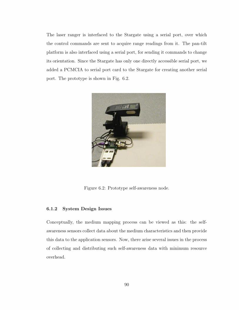
The laser ranger is interfaced to the Stargate using a serial port, over which
the control commands are sent to acquire range readings from it. The pan-tilt
platform is also interfaced using a serial port, for sending it commands to change
its orientation. Since the Stargate has only one directly accessible serial port, we
added a PCMCIA to serial port card to the Stargate for creating another serial
port. The prototype is shown in Fig. 6.2.
Figure 6.2: Prototype self-awareness node.
6.1.2 System Design Issues
Conceptually, the medium mapping process can be viewed as this: the self-
awareness sensors collect data about the medium characteristics and then provide
this data to the application sensors. Now, there arise several issues in the process
of collecting and distributing such self-awareness data with minimum resource
overhead.
90

First, the range data must be collected as fast as possible, in order to enable
faster updates and to minimize the node active time. The naıve method would be
to take a range measurement at a sufficiently fine granularity and determine which
regions are blocked from view. However, the environment has certain structure
to it and it is intuitive to expect that if such structure can be exploited, we
can reduce the number of readings to be collected, thereby speeding up the data
acquisition process. Implementing this procedure on a practical laser ranger and
pan-tilt platform reveals the various issues in doing this. Our aim is to determine
useful strategies to minimize data acquisition time, which are expected to work
in a wide variety of environments in view of the system limitations.
Second, the medium map has a significant data size. This motivates a study of
efficient methods for sharing this data among the application and self-awareness
nodes. The storage and communication strategies may attempt to minimize the
data size, but the compression techniques should not lead to extensive processing
overheads for retrieval and update. The storage strategies for a data set typi-
cally depend upon the nature of queries that must be answered using the stored
data. Our objective is to determine the relevant strategies to store and share
medium map data in a manner that enables answering queries about the medium
occlusions for the application sensors.
There are further design steps required to complete the self-awareness process.
The medium information may have to be appropriately converted to a form that
enables the application sensor to determine which portions of its field of view are
occluded. For instance, in our test-bed the spatial coordinates of an obstacle may
have to be mapped to the corresponding pixel coordinate in the image taken by
a camera. For the case of cameras, this process is known as external calibration
and existing methods [HS97] can be used for this step.
91

Also, since the self-awareness sensors are not necessarily present at the ap-
plication sensor node and a single self-awareness node will typically not be able
to map the entire medium, self-awareness data from multiple nodes has to be
combined to develop a coherent medium map. In our test-bed we assume that
each node is localized, in a common coordinate system. Such an assumption is
valid for sensor networks since most nodes are static and localization is a basic
service required for many other sensor network applications. Given the location
information, the medium data from different locations can be combined using the
appropriate spatial transformations and we do not dwell on it further.
6.1.2.1 Technology Choice
We have selected a laser range sensor to measure the medium characteristics.
There are other means to achieve the same functionality. One alternative is to
use stereo-vision to derive depth maps. This approach has limitations of accuracy
compared to a laser sensor and may miss small obstacles in the environment. Also,
stereo-vision algorithms require detecting key features in the environment which
can then be identified in the multiple images collected by the cameras in the
stereo-system. It may not work in all environments where such key features are
hard to detect. Further, the stereo-vision generated depth map is relative and
a known dimensional measure is required in the environment to scale the depth
measurements correctly.
These issues motivated us to use a range sensor. Among range sensors, there
are various options, such as ultrasound ranging and infra-red ranging. Both these
alternatives give lower accuracy than the laser, and the distance range of the infra-
red sensors is usually lower than that of laser based ones. However, both these
are usually available at a lower cost, and may be of interest in scenarios where
92

the low accuracy is not a deterrent. The map acquisition algorithms discussed in
later sections are in fact applicable to these types of range sensors as well. The
data sharing methods developed in our prototype are applicable to all the above
alternatives.
Advanced three dimensional imaging technologies, such as based on single
photon avalanche devices [NRB04] may make three dimensional imaging more fea-
sible in the future. This may yield more alternatives to realize the self-awareness
sensing functionality that we propose for sensor networks.
Mapping based on range sensors has also been considered in mobile robot nav-
igation. While our problem is similar, the solution is different and the resultant
design issues are distinct. For a robot, medium mapping is a primary task nec-
essary for navigation. Even if the environment map were available a-priori, the
range sensor on a robot would be actively used to avoid obstacles in the path. In
the case of a sensor network, the demands from the self-awareness sensor are less
stringent. First, the self-awareness data is not being used for active navigation
of a mobile robot. Each node need not have a self-awareness sensor. The static
nature of most sensor nodes also enables carrying out the mapping process at a
much slower pace than required for a robot. A direct consequence of this is in
the technology choice – the laser range sensor used in our work is significantly
cheaper than those typically used on robots and has a slower response time for
taking range readings. The pan-tilt actuation used in our prototype is much
slower than required for real time navigation, and can be achieved with lower
energy expenditure. Second, the assumption on the availability of localization
also causes our work to differ significantly from robotic mapping. In the case of
a team of multiple robots exploring an unknown environment, the processes of
localization and mapping are dependent [DNC01] on each other. Combining the
93

maps generated at multiple robots is not straightforward and different techniques
such as maximum sub-graph isomorphism have been explored for that purpose.
On the other hand, for sensor networks, if localization is available as is needed for
many sensor network applications, combining the self-awareness data from mul-
tiple nodes is simpler. Thus, the medium mapping problem in sensor networks
is more tractable than the corresponding robotics problem, and we expect to be
able to solve it with a lower resource overhead.
6.1.3 Adaptive Medium Mapping
There are three basic types of maps [Cho]:
1. Grid based: These maps divide the space into discrete elements which are
mapped as empty or occupied [ME85, TB96].
2. Feature based: These maps are a collection of landmark features in the
environment [SSC90, LDC92].
3. Topology based: These maps represent distinctive places in the environment
as nodes in a graph and the interconnections or paths between them as the
edges [KW94, RN99].
For the purpose of determining sensing occlusions, the most relevant maps are the
grid based ones. These provide a detailed model of the sensing medium, based
on which the application sensors may estimate their sensing performance.
The process to generate a grid based medium map proceeds as follows. Range
measurements are taken by orienting the laser at varying pan and tilt from a fixed
location to form a depth map for the space around the self-awareness node. Such
depth maps from multiple self-awareness nodes may then be combined to develop
94
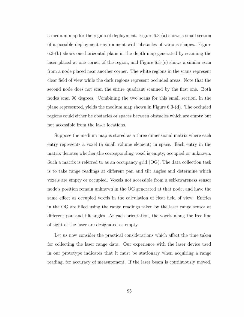
a medium map for the region of deployment. Figure 6.3-(a) shows a small section
of a possible deployment environment with obstacles of various shapes. Figure
6.3-(b) shows one horizontal plane in the depth map generated by scanning the
laser placed at one corner of the region, and Figure 6.3-(c) shows a similar scan
from a node placed near another corner. The white regions in the scans represent
clear field of view while the dark regions represent occluded areas. Note that the
second node does not scan the entire quadrant scanned by the first one. Both
nodes scan 90 degrees. Combining the two scans for this small section, in the
plane represented, yields the medium map shown in Figure 6.3-(d). The occluded
regions could either be obstacles or spaces between obstacles which are empty but
not accessible from the laser locations.
Suppose the medium map is stored as a three dimensional matrix where each
entry represents a voxel (a small volume element) in space. Each entry in the
matrix denotes whether the corresponding voxel is empty, occupied or unknown.
Such a matrix is referred to as an occupancy grid (OG). The data collection task
is to take range readings at different pan and tilt angles and determine which
voxels are empty or occupied. Voxels not accessible from a self-awareness sensor
node’s position remain unknown in the OG generated at that node, and have the
same effect as occupied voxels in the calculation of clear field of view. Entries
in the OG are filled using the range readings taken by the laser range sensor at
different pan and tilt angles. At each orientation, the voxels along the free line
of sight of the laser are designated as empty.
Let us now consider the practical considerations which affect the time taken
for collecting the laser range data. Our experience with the laser device used
in our prototype indicates that it must be stationary when acquiring a range
reading, for accuracy of measurement. If the laser beam is continuously moved,
95
(a) Sample Deployment Environment
0 0.5 1 1.5 2 2.5 30
0.5
1
1.5
2
2.5
3
(b) Depth map A
0 0.5 1 1.5 2 2.5 30
0.5
1
1.5
2
2.5
3
(c) Depth map B
0 0.5 1 1.5 2 2.5 30
0.5
1
1.5
2
2.5
3
(d) Medium map
Figure 6.3: Map generation process.
the device still returns range measurements. However, the time taken to acquire a
range reading increases by an unpredictable amount, which makes it is impossible
96
to determine the orientation, and hence the relevant voxels in the OG, which
corresponds to the returned range reading. Thus, the laser is moved in small
steps along the pan and tilt axis and the readings are acquired when the device
is stationary. With this, the time taken, T, to acquire a reading at a particular
pan and tilt position can be modeled as consisting of three components:
T = tmove + taxdx + tread (6.1)
where tmove represents the time taken by the pan-tilt platform to move to the next
position at a constant speed using the pan and tilt motors, taxdx represents the
additional time taken due to acceleration and deceleration phases in executing
the motion step since constant speed cannot maintained throughout the motion,
and tread represents the time taken for the laser range sensor to acquire a reading.
The parameters tmove and taxdx depend on the capabilities of the pan-tilt
platform, and tread depends on the laser unit, and the reflectivity and the angle
of incidence of the surface at which the laser beam is pointed. For a constant
pan and tilt range scanned by the laser at a given granularity, suppose the total
angular distance moved is dω and the number of readings taken is N . The total
time taken to execute the scan becomes:
Tscan = dω ∗ tmove + N{taxdx + tread} (6.2)
The time taken thus varies with N . If we reduce N , and thus increase the angular
step size at which the laser stops to take a reading, Tscan can be reduced. Our
objective is to generate the OG in a manner that exploits the structure in the
environment in order to reduce the number of readings taken by the laser.
97
6.1.4 Reducing the Scan Time
For many signals, a frequency spectrum analysis yields that the signal needs to be
sampled only at a coarse granularity. Considering the range scan in space as the
signal to be sampled (such as shown in Fig 6.3-(b,c)), indicates that the Nyquist
sampling interval is quite small due to the presence of sharp discontinuities in the
environmental features, and the value of N derived in this manner is very high.
Thus, we need to exploit other forms of structure in this signal. We propose
two heuristics to exploit such structure. These are described in terms of the pan
motion of the laser1 and the goal is to minimize the number of readings for a
constant pan scan range.
6.1.4.1 Adaptive Filter Based Algorithm
The first method is based on the use of an adaptive filter to learn the medium
structure from the readings acquired and when the laser readings match those
predicted based on the adaptive filter, the scan step size may be increased to
reduce the number of points measured. We refer to this method as adaptive
filter based (AFB) algorithm and use least-mean-square (LMS) adaptation as our
adaptive filter. LMS is a gradient descent based heuristic for the filter adaptation.
Suppose the filter at time step i is represented by a length n column vector h(i),
the previous n values of the scan are represented by a column vector x(i), and
e(i) is the error in the prediction, calculated using:
e(i) = hT (i)x(i)− x(i + 1) (6.3)
1Similar methods apply to tilt motion.
98

where x(i + 1) is the measurement at time step (i + 1). Then the gradient search
equation to minimize the square-error becomes:
h(i + 1) = h(i)− µ▽ (|e(i)|2) (6.4)
where the gradient ▽(·) is taken with respect to filter coefficients h, and µ is
a constant step size for the gradient descent. Simplifying the above expression
leads to a computationally efficient filter update equation:
h(i + 1) = h(i)− µe(i)x(i) (6.5)
We deviate slightly from the conventional LMS filter in that the step size at
which readings are taken varies as we adapt the angular step size using the AFB
algorithm. Whenever the prediction error e(i) is below a threshold, we increase
the angular step size for the laser pan motion, as described in the next subsection.
The step size cannot be increased beyond a certain limit which depends on the
size of the smallest feature of interest to be mapped. The problem of adaptive
filter design is not addressed as part of this work; several adaptive filters are
available, and may be explored depending on the specific needs of the system
[Hay01].
6.1.4.2 Adaptive Linear Prediction Algorithm
The second method is more domain specific and exploits the nature of the signal
being sampled. Since adaptive filters are not specially designed for depth maps,
they require significant learning data. However, observe that when sampling at a
fine granularity, many of the surfaces in the medium, especially for indoor built
environments, can be approximated as consisting of small planes, or in one plane
of pan motion, a curve consisting of small line segments. When scanning this
curve, the number of samples taken need only be sufficient to reproduce the line
99

segments. Thus, when range data indicates that the laser is taking measurements
along a line, we may increase the angular step size of the pan motion.
This prediction method proceeds as follows: Determine the coordinates of the
points on the sampled curve corresponding to the previous two range readings.
Use these to determine the equation of the line joining them. Now predict the
coordinates of the next point along this line, which the laser will hit when moved
by its current angular step size. At the next laser pan step, calculate the error
between the predicted point and the measured point. If the error is below a
threshold, increase the angular step size. The exact algorithm to control the step
size appears in the next subsection. We will refer to this method as the adaptive
linear prediction (ALP) algorithm.
Some further improvements can be applied to both the AFB and ALP algo-
rithms as described below.
First, when the laser range extends beyond the area of interest, such as when
the laser is near an edge of the deployment area, we need not scan the exact
structure of the medium and may increase the angular step size to the maximum
limit dictated by the minimum obstacle size to be detected. The step size would
be reduced as soon as a feature of interest is detected within the region of interest.
Second, for a given angular step size, the scan resolution in space varies with
distance from the laser. This can be seen in Fig. 6.4: the spatial resolution ∆α is
higher than ∆β for the same angular step ∆θ. Thus, ∆θ may be increased when
scanning obstacle A, as the OG is stored at a constant resolution in space.
Third, when the step size has been increased using an adaptive method and
a high error is encountered, it is likely that a large change in the scanned depth
occurred in the region between the current and the previous readings. Thus, if
we back-track, i.e., move the laser back to the previous position and then scan
100

∆θ ∆β
∆θB
∆αA
Figure 6.4: Varying spatial resolution with obstacle distance.
the region of large change using a small step size, the quality of reproduction can
be improved significantly with a small increase in the number of readings taken.
6.1.5 Algorithm Implementation and Evaluation
The precise ALP and AFB algorithms derived from the above discussion are
stated together in Fig. 6.5. The key difference among the two algorithms is in
the prediction step. The values of parameters used are summarized in Table 6.1.
The parameter ∆θ0 represents the minimum angular step size required to achieve
a desired spatial resolution, for the maximum laser range in the environment.
The step size µ was chosen to be 0.03. Larger step sizes were tried, and while
they yield faster convergence and somewhat lower error, they lead to divergence
of the LMS filter in some cases. The filter length was kept at n = 3. A larger filter
length can learn more complex shapes but needs a longer adaptation time and
the signal characteristics may change over such time as the laser moves from one
obstacle to another with different a shape. Optimizing the LMS filter for various
environment categories is part of future work. We now evaluate these algorithms
by comparing them to a constant step size approach, both using simulations,
which allows testing over several obstacle placements, and using experiments on
our prototype hardware.
101
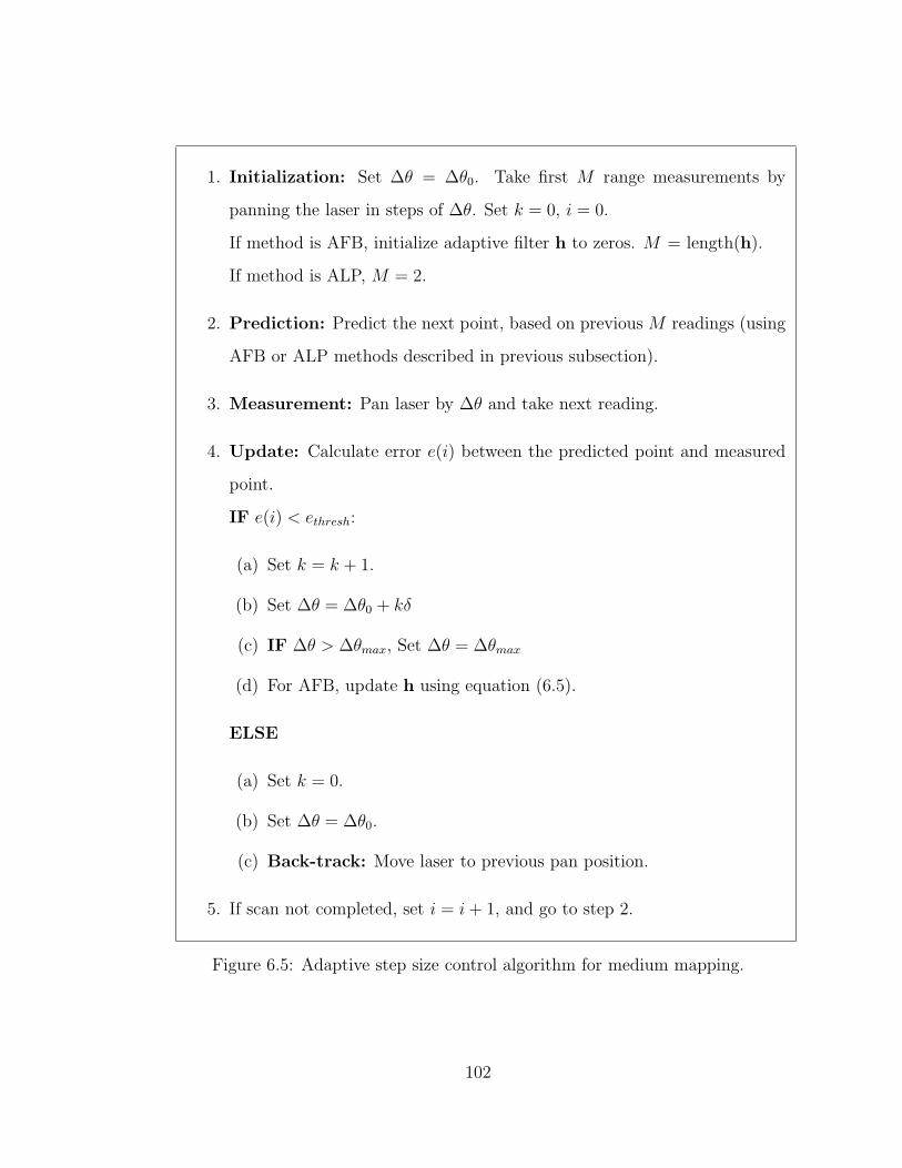
1. Initialization: Set ∆θ = ∆θ0. Take first M range measurements by
panning the laser in steps of ∆θ. Set k = 0, i = 0.
If method is AFB, initialize adaptive filter h to zeros. M = length(h).
If method is ALP, M = 2.
2. Prediction: Predict the next point, based on previous M readings (using
AFB or ALP methods described in previous subsection).
3. Measurement: Pan laser by ∆θ and take next reading.
4. Update: Calculate error e(i) between the predicted point and measured
point.
IF e(i) < ethresh:
(a) Set k = k + 1.
(b) Set ∆θ = ∆θ0 + kδ
(c) IF ∆θ > ∆θmax, Set ∆θ = ∆θmax
(d) For AFB, update h using equation (6.5).
ELSE
(a) Set k = 0.
(b) Set ∆θ = ∆θ0.
(c) Back-track: Move laser to previous pan position.
5. If scan not completed, set i = i + 1, and go to step 2.
Figure 6.5: Adaptive step size control algorithm for medium mapping.
102

Parameter Value
ethresh 1 cm
µ 0.03
length(h) 3
δ 0.05◦
∆θmax ∆θ0 + 1◦
Table 6.1: Algorith parameter values.
6.1.5.1 Simulations
To test the proposed methods, we generate several random obstacle placements
in a square region, place the laser ranger in one corner of the square and simulate
the range readings that would be collected when the laser is panned with the
step size computed as per the adaptive methods. As a base case, the readings
are also generated if the laser were to be panned with a periodic step size kept
at ∆θ0. The obstacles generated are rectangles and circles, placed randomly and
overlapping with each other leading to arbitrary shaped obstacles, such as shown
in Fig. 6.6(a). Ten such random obstacle topologies were generated. A simulated
laser scan using adaptive step sizes is shown in Fig. 6.6(b), where the varying
step size between successive pan positions is apparent, and the back-tracking near
obstacle edges may be seen as well. The angular step size increases as the filter
learns a curve and falls back again when the curve changes significantly.
Error performance of a scan is calculated as follows. From the application
perspective, the OG generated from the range scan data is of interest. A high
resolution periodic scan is first carried out and the OG generated from it is
used as the ground truth. Then, for each simulated scan, the corresponding
OG is generated and the error is measured in terms of the number of voxels
103

which differ with respect to the ground truth OG. A two dimensional OG is used
for the simulations, considering only the pan motion of the laser. The exact
same techniques can be applied in the tilt direction as well to generate the three
dimensional OG. The number of differing pixels is normalized by the number of
total pixels in the OG, and the error is plotted as a percentage.
For each topology, multiple scans are carried out with ∆θ0 varying from 0.09◦
to 0.9◦. Increasing ∆θ0 implies reducing the resolution of the scan and thus
increasing the error. For each scan, we count the number of readings taken when
a periodic scan is used and when the adaptive algorithms are used. To compare
the savings in time when using the adaptive methods, we plot the number of
readings taken for the same error using the periodic and adaptive schemes.
The simulation data needs to be averaged over the random topologies. Since
each topology may lead to different error values with varying ∆θ0, the number of
readings, N , required cannot be directly averaged. We divide the error axis into
small intervals and consider the average of number of readings taken for error
across multiple topologies divided into these intervals. These averaged plots are
shown in Fig. 6.6(c). The error-bars show the standard deviation across multiple
topologies.
The figure shows that at low error the adaptive scans require much fewer
readings than the periodic scan. Among AFB and ALP, ALP performs better
since it is designed specifically for the nature of the sampled signal. As the angle
step is increased for the periodic scan, the error increases and the number of
readings reduces. However, the advantage due to adaptive methods dwindles as
the step size for the periodic scan has also increased. The portions of the scan
where the adaptive methods can use an increased step size now form a smaller
fraction of the total scan.
104

0 0.5 1 1.5 2 2.5 30
0.5
1
1.5
2
2.5
3
(a) Sample deployment
0 0.5 1 1.5 2 2.5 30
0.5
1
1.5
2
2.5
3
(b) Sample AFB scan
0.1 0.2 0.3 0.4 0.5 0.6100
200
300
400
500
600
700
800
Error (%)
Num
ber
of R
eadi
ngs
ALPAFBPeriodic
(c) Error performance
Figure 6.6: Comparing the number of readings taken with varying error perfor-
mance for the three scanning strategies.
6.1.5.2 Experiment
We now experimentally compare the performance of these algorithms using our
prototype self-awareness node. Apart from validating the implementation of our
proposed methods on an embedded platform, the experiments include additional
effects not modeled in the simulations. First is the presence of sensing errors in
the laser readings and pan motion. Secondly, while in the simulation, only the
number of readings could be plotted, in the experiment we can measure the total
105

savings in time. These includes the time for motion and the time for taking a laser
reading. The time for taking a laser reading varies with the color of the surface
scanned and even for the same number of readings, the difference in the positions
of those readings on some dark colored spots in the environment may cause an
increase in time consumed; such effects were not modeled in the simulation.
The environment used in our experiment was a 2m square space with some
objects placed as obstacles. The results are shown in Fig. 6.7. Only the better
adaptive method, ALP, was used.
0.2 0.3 0.4 0.5 0.6 0.7 0.8 0.9 1 1.1100
200
300
400
500
600
700
Tim
e (s
)
Error (%)
ALPPeriodic
Figure 6.7: Comparing the adaptive and periodic scan strategies using the pro-
totype self-awareness node.
These results are similar to those seen in simulations. The evaluation clearly
shows that significant savings in time can be achieved using the adaptive methods.
Apart from the savings in time, another side effect of the adaptive methods
is a saving in storage and communication overhead as discussed next.
106

6.1.6 Sharing the Self-awareness Data
After each laser sensor has collected the range scan, using either a periodic scan
or the adaptive methods, the data at each self-awareness node must be used to
determine the medium occlusions at each application node. There are several
design choices in doing this, differing in how the data is stored and how the
depth maps from multiple laser sensors are combined.
Data-sharing schemes depend on the nature of queries that need to be an-
swered based on the stored data. In our system, the application sensors are only
interested in determining the occluded regions from their point of view. The
individual occupancy grid (OG) generated by a laser scan (such as seen in Fig.
6.3(b)) may be stored at each laser node. To generate the medium map all laser
nodes with overlapping fields of view must transmit their OG’s to a common
location where the medium map is then computed. The individual OG’s are first
translated along the spatial axes in a global reference frame, depending on the
laser coordinates and then an ‘OR’ of their overlapping voxels is computed. The
OR operation assumes that the occluded voxels (obstacle surfaces or unknown)
are stored as zeros and the clear regions as ones. This generates a combined OG,
referred to as the medium map (as was seen in Fig. 6.3(d)). Relevant portions of
such a medium map once generated can be distributed to each application sensor.
6.1.6.1 Computing the Field of View at Application Sensors
We can improve the above process if we observe that the medium map need not
be calculated centrally for the application sensors to be able to calculate their
occlusions. Each self-awareness node need not compute its OG, but may just
store the raw coordinates of the points scanned by the laser ranger. Let us refer
to these points as range coordinates. The range coordinates which were used
107

to compute the OG’s seen in Figures 6.3(b) and 6.3(c) are shown in Figures
6.8(a) and 6.8(b). We present a distributed method using which the raw range
0 0.5 1 1.5 2 2.5 3
0
0.5
1
1.5
2
2.5
3
Laser A
(a) Range coordinates A
0 0.5 1 1.5 2 2.5 3
0
0.5
1
1.5
2
2.5
3
Laser B
(b) Range coordinates B
Figure 6.8: Range coordinates used to compute occupancy grids (OG’s)
coordinates at the individual laser nodes are directly used by the application
sensors to determine their occlusions.
Suppose the nominal range of the laser is known to be Rl, and that of the
application sensor is Rs; the actual ranges may be much shorter due to presence
of obstacles. An application sensor now accesses those laser nodes which are
within Rl distance, and queries the range coordinates stored by the laser, as well
as the coordinates of the laser itself. The application sensors now computes their
own OG’s, to represent which voxels in their field of view are unoccupied, as
follows: connect the laser node coordinates to each of the range coordinates, and
all voxels through which the connecting lines pass are deemed to be unoccupied.
The application sensor only generates the OG for a circular area of radius Rs
around it and not the entire Rl.
As an illustration, consider the 3m× 3m area seen in Fig. 6.3 and the corre-
sponding range coordinates in Fig. 6.8. Laser A was placed at (x, y) = (0, 0) and
108

laser B was placed at (2.22, 2.15). Suppose an application sensor, say, a camera
with full 360◦ pan range, is placed at (0.5, 1), and has Rs = 1. It first accesses
the range coordinates from laser A and computes its local OG by checking which
pixels are unoccupied, as shown in Fig. 6.9(a). The OG is computed at a reso-
lution of 1cm, which means that each grid point in the OG is separated by 1cm.
Next, it accesses the range coordinates from laser B. Again, it connects the range
0 50 100 1500
20
40
60
80
100
120
140
160
180
200
x (cm)
y (c
m)
Sensor
(a) OG, using laser A
0 50 100 1500
20
40
60
80
100
120
140
160
180
200
x (cm)y
(cm
)
Sensor
(b) OG, using lasers A and B
Figure 6.9: Example: Generating a combined OG directly at the application
sensor.
coordinates with the laser coordinates and computes the unoccupied pixels, thus
discovering further pixels in its OG which are unoccupied. This OG is seen in
Fig. 6.9(b).
6.1.6.2 Evaluation
In our proposed approach, no global medium map is generated. This approach
has several advantages compared to the laser nodes first generating their OG’s,
exchanging them, generating the medium map and then distributing it to the
application sensors.
109

Memory Requirements: The application sensors calculate the OG only
within their sensing range, Rs. The size of the OG is proportional to the cube
of Rs (or the square of Rs when only the horizontal plane is considered). If
Rs < Rl, which is the case in our system, this means that each application sensor
has to compute a much smaller OG than at a laser node. This is significant,
since embedded nodes have limited memory, and increasing the memory size in
increases their power consumption and cost.
Communication and Storage Overhead: The communication overhead
in our approach is only the data-size of the range coordinates. This is significantly
lower than the OG at a laser, and the combined OG’s (medium maps) generated
using the data from multiple lasers. For instance, at a resolution of 1cm, the
size of the OG matrix in two dimensions is 104 binary values per square meter,
while the range coordinates only store a few points corresponding to obstacles
in the same area. The number of points stored can further be reduced using the
adaptive methods discussed in the previous sections.
It may be noted that the OG need not be communicated in its raw form but
could be compressed using a data compression or image compression method.
Our approach of storing range coordinates can be viewed as a domain specific
compression scheme which is expected to perform better than the general com-
pression techniques. Fig. 6.10 shows the storage space required for our proposed
approach with Periodic, AFB, and ALP methods, as well as that required for
storing the OG when using a data compression technique: TIF-packbits com-
pression, which is a lossless compression method exploiting the repetition of bits,
and an image compression technique: JPEG, which uses a transform to derive an
efficient data representation. The sizes are for the same data sets as generated in
the previous section.
110
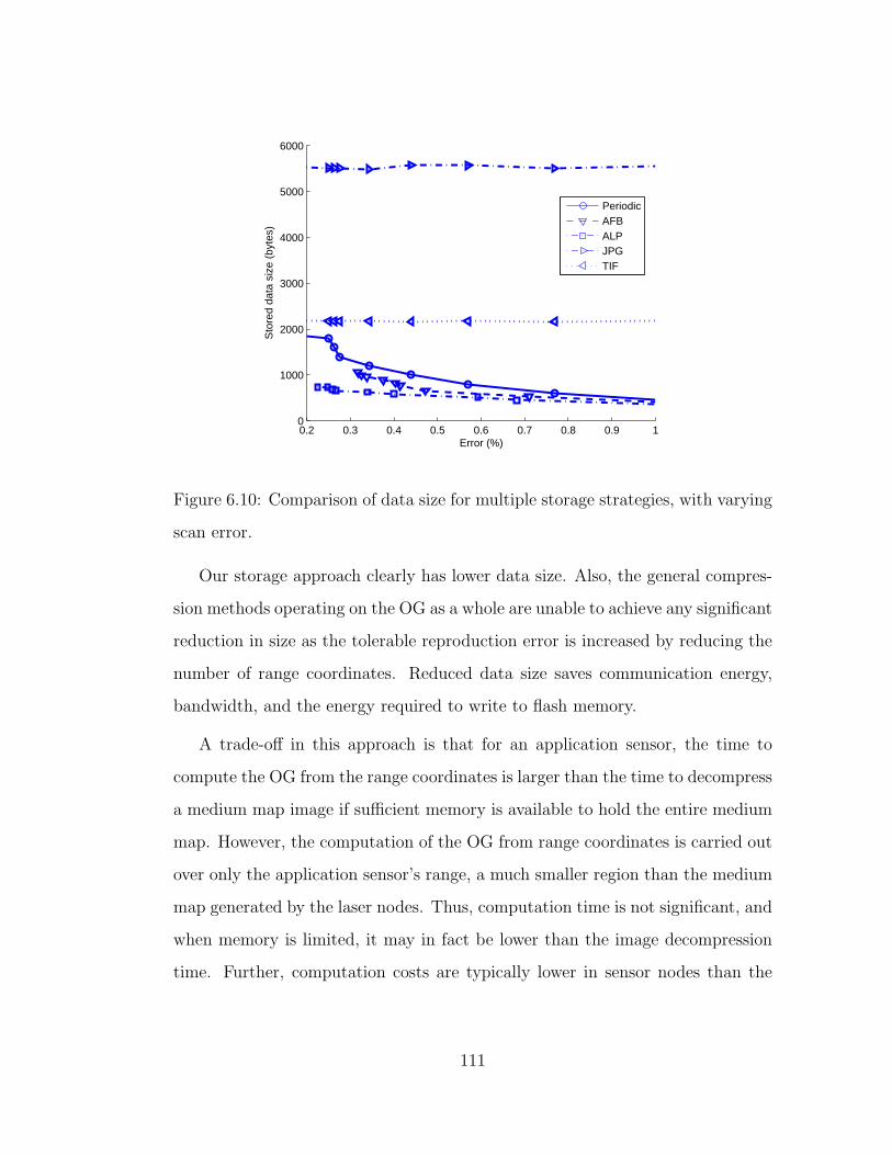
0.2 0.3 0.4 0.5 0.6 0.7 0.8 0.9 10
1000
2000
3000
4000
5000
6000
Error (%)
Sto
red
data
siz
e (b
ytes
)
PeriodicAFBALPJPGTIF
Figure 6.10: Comparison of data size for multiple storage strategies, with varying
scan error.
Our storage approach clearly has lower data size. Also, the general compres-
sion methods operating on the OG as a whole are unable to achieve any significant
reduction in size as the tolerable reproduction error is increased by reducing the
number of range coordinates. Reduced data size saves communication energy,
bandwidth, and the energy required to write to flash memory.
A trade-off in this approach is that for an application sensor, the time to
compute the OG from the range coordinates is larger than the time to decompress
a medium map image if sufficient memory is available to hold the entire medium
map. However, the computation of the OG from range coordinates is carried out
over only the application sensor’s range, a much smaller region than the medium
map generated by the laser nodes. Thus, computation time is not significant, and
when memory is limited, it may in fact be lower than the image decompression
time. Further, computation costs are typically lower in sensor nodes than the
111
costs of flash memory writes and communications, and hence this approach is
still preferred.
Resolution Flexibility: The application sensor is free to compute its field
of view at a much lower resolution than the data generated at the laser. Without
application information, the laser node may have to compute the medium map
at the highest resolution possible with the collected data, and generate a much
larger OG matrix than required.
Reduced Remote State Dependence: The proposed method is com-
pletely distributed, and dependence on the state of remote nodes is minimal.
Firstly, no data exchange is required among the self-awareness nodes. Since Rl
may be large, such communication may have required data to be sent over large
distances. Reducing this overhead saves significant bandwidth. Secondly, the
application sensors are not required to know the state of progress of the self-
awareness nodes coordination and determine if the combined medium map has
been generated. They may access each self-awareness node’s data asynchronously.
Such reduced state dependence not only simplifies design in distributed systems
but also helps improve system robustness because in case of a node’s failure, its
effect on other nodes is reduced. The modular and decoupled operation yields a
significant advantage when the sensor network is executing multiple applications
and services.
Efficient Updates: The medium may change over time and our data sharing
method allows for efficient updates. First, transmitting only the range coordi-
nates to the application sensors reduces the size of data communicated. This
approach has at least as much advantage in communication overhead as seen in
Figure 6.10 with respect to the size of the update data to be exchanged. Sec-
ond, the asynchronous data access mode, rather than having to wait for the
112
self-awareness nodes to generate a coherent map, allows for update information
to be incrementally incorporated with minimal delay as and when the medium
changes.
The updates may be exchanged using either a push or a pull approach. In the
push approach, the laser nodes send an update to the application sensor whenever
a change is detected and in the pull approach, the application sensor queries
the laser nodes for updates. Depending upon the nature of the deployment,
one of these methods would be preferred. For instance, if the medium changes
infrequently, then the self-awareness nodes may push the updates. This saves
the overhead of the application nodes periodically polling for updates when not
many updates are expected. However, if medium changes are frequent, the push
approach will lead to a high overhead. In this case, the application sensors should
query for updates at the frequency they require. The pull approach is also useful
for power management as it allows application sensors to enter low power modes
without worrying about medium changes when they are not even sensing. In our
system we have selected the pull approach to keep the update process at each
application sensor decoupled from the self-awareness node’s operation. The laser
periodically collects data and publishes it at a known location. In our prototype,
we use the common HTTP protocol for data exchange. The range coordinate data
is stored in a web accessible folder on the self-awareness node. The application
sensors access this data as required.
There are other enhancements possible to the update process if the overhead of
maintaining remote nodes’ state is acceptable. For instance, each self-awareness
node may maintain the locations of the application sensors which access it. Then,
it could compute which portions of its range coordinate data affect each appli-
cation sensor. In case of updates to the range coordinates data, the laser would
113
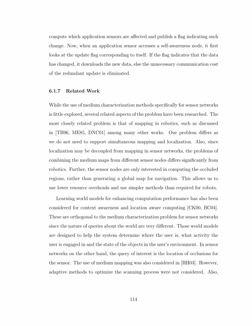
compute which application sensors are affected and publish a flag indicating such
change. Now, when an application sensor accesses a self-awareness node, it first
looks at the update flag corresponding to itself. If the flag indicates that the data
has changed, it downloads the new data, else the unnecessary communication cost
of the redundant update is eliminated.
6.1.7 Related Work
While the use of medium characterization methods specifically for sensor networks
is little explored, several related aspects of the problem have been researched. The
most closely related problem is that of mapping in robotics, such as discussed
in [TB96, ME85, DNC01] among many other works. Our problem differs as
we do not need to support simultaneous mapping and localization. Also, since
localization may be decoupled from mapping in sensor networks, the problems of
combining the medium maps from different sensor nodes differs significantly from
robotics. Further, the sensor nodes are only interested in computing the occluded
regions, rather than generating a global map for navigation. This allows us to
use lower resource overheads and use simpler methods than required for robots.
Learning world models for enhancing computation performance has also been
considered for context awareness and location aware computing [CK00, BC04].
These are orthogonal to the medium characterization problem for sensor networks
since the nature of queries about the world are very different. Those world models
are designed to help the system determine where the user is, what activity the
user is engaged in and the state of the objects in the user’s environment. In sensor
networks on the other hand, the query of interest is the location of occlusions for
the sensor. The use of medium mapping was also considered in [HH03]. However,
adaptive methods to optimize the scanning process were not considered. Also,
114
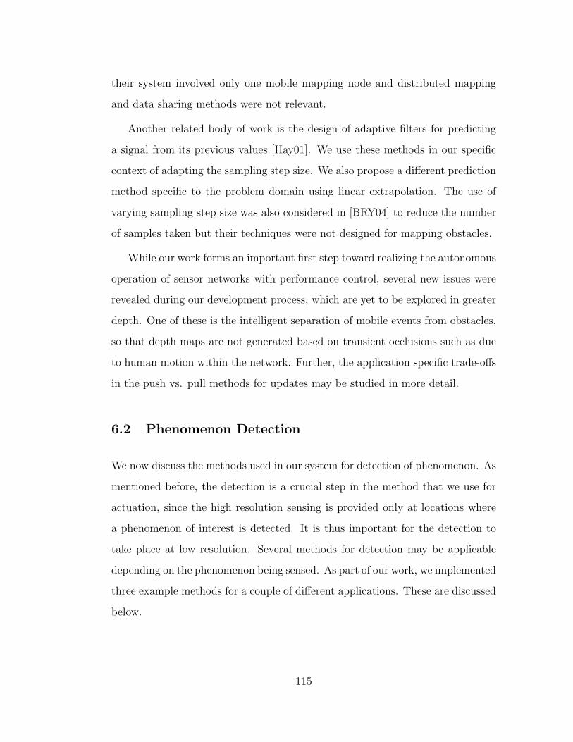
their system involved only one mobile mapping node and distributed mapping
and data sharing methods were not relevant.
Another related body of work is the design of adaptive filters for predicting
a signal from its previous values [Hay01]. We use these methods in our specific
context of adapting the sampling step size. We also propose a different prediction
method specific to the problem domain using linear extrapolation. The use of
varying sampling step size was also considered in [BRY04] to reduce the number
of samples taken but their techniques were not designed for mapping obstacles.
While our work forms an important first step toward realizing the autonomous
operation of sensor networks with performance control, several new issues were
revealed during our development process, which are yet to be explored in greater
depth. One of these is the intelligent separation of mobile events from obstacles,
so that depth maps are not generated based on transient occlusions such as due
to human motion within the network. Further, the application specific trade-offs
in the push vs. pull methods for updates may be studied in more detail.
6.2 Phenomenon Detection
We now discuss the methods used in our system for detection of phenomenon. As
mentioned before, the detection is a crucial step in the method that we use for
actuation, since the high resolution sensing is provided only at locations where
a phenomenon of interest is detected. It is thus important for the detection to
take place at low resolution. Several methods for detection may be applicable
depending on the phenomenon being sensed. As part of our work, we implemented
three example methods for a couple of different applications. These are discussed
below.
115

6.2.1 Ellipse Detection
One of the example applications for a network of cameras such as our system
is to detect objects of interest in a user’s environment for various ubiquitous
computing applications. One approach for detecting objects using cameras is to
place a visual tag on each object of interest. Methods have already been proposed
to design tags and recognize a tag given a high resolution image of the tag[IL01].
Our system can thus provide the sensing infrastructure required to obtain the
high resolution images.
An example tag used in the tag recognition system developed in [IL01] is
shown in Figure 6.11.
Figure 6.11: Example visual tag used for object detection.
The circular pattern seen in the tag is a visual code for an identification
number. The exact pattern of the tag depends on the identification number
which is to be represented. The tag design is such that it has two concentric
circles in the middle of the pattern. These concentric circles are common for any
tag number and are used to detect the tag in the field of view of the camera.
The circles may appear as ellipses depending on the angle which the plane of
116
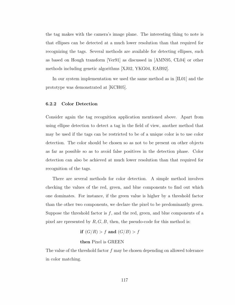
the tag makes with the camera’s image plane. The interesting thing to note is
that ellipses can be detected at a much lower resolution than that required for
recognizing the tags. Several methods are available for detecting ellipses, such
as based on Hough transform [Ver91] as discussed in [AMN95, CL04] or other
methods including genetic algorithms [XJ02, YKG04, EAB92].
In our system implementation we used the same method as in [IL01] and the
prototype was demonstrated at [KCH05].
6.2.2 Color Detection
Consider again the tag recognition application mentioned above. Apart from
using ellipse detection to detect a tag in the field of view, another method that
may be used if the tags can be restricted to be of a unique color is to use color
detection. The color should be chosen so as not to be present on other objects
as far as possible so as to avoid false positives in the detection phase. Color
detection can also be achieved at much lower resolution than that required for
recognition of the tags.
There are several methods for color detection. A simple method involves
checking the values of the red, green, and blue components to find out which
one dominates. For instance, if the green value is higher by a threshold factor
than the other two components, we declare the pixel to be predominantly green.
Suppose the threshold factor is f , and the red, green, and blue components of a
pixel are rpresented by R,G,B, then, the pseudo-code for this method is:
if (G/R) > f and (G/B) > f
then Pixel is GREEN
The value of the threshold factor f may be chosen depending on allowed tolerance
in color matching.
117

A second method is based on a computation of the Euclidean distance between
the color of the test pixel and the reference color. Suppose the reference color to
be detected is represented by a vector [Rf , Gf , Bf ]. Suppose the test pixel has a
value [R,G,B]. Then, the Euclidean distance, D, is:
D =√
(R−Rf )2 + (G−Gf )2 + (B −Bf )2 (6.6)
The reference color may be picked to match the tag color, say green, represented
by [Rf , Gf , Bf ] = [0, 255, 0]. The detection procedure compares the distance, D,
with an allowed tolerable error threshold and if D is smaller than the threshold,
the color is declared to match.
More advanced methods are available based on transformations of the pixel
vectors. For instance, pixel values in the red, green, and blue (RGB) format may
be converted to the hue, saturation, and value (HSV) vector space, where the hue
specifies the color and the saturation value may be used to allow for tolerances
in the purity of the color. Several color detection techniques are surveyed in
[VSA03].
In our system we used threshold based color detection, with f = 1.5, and
implemented it for two different colors: green and red. The implemented system
was demonstrated at [KCK05b].
6.2.3 Motion Detection
As another application consider logging high resolution images of all vehicles
entering a particular campus area, as shown in Figure 1.1 in chapter 1. One
method to detect vehicles using low resolution coverage is to use motion detection.
We implemented motion detection methods specifically to detect vehicles as part
of our work.
118

The processing carried out to detect moving vehicles in the image data is
described below.
1. A background image is first captured to be used as prior knowledge of the
scene being photographed. This background image is updated using an
autoregressive filter as described in [SDB00]. The update step for each
pixel I(i, j) in the image matrix is:
I(i, j) = a ∗ Icaptured(i, j) + (1− a) ∗ I(i, j) (6.7)
where Icaptured denotes the most recently captured image while I is the
maintained background image. The parameter a satisfies 0 ≤ a ≤ 1 and
is typically close to zero. A larger value will lead to a faster update but
will also cause some of the motion events to be incorporated into the back-
ground. We use a = 0.05. The objective of the update is to to adapt the
background image to gradual changes such as due to light variations or
addition of background objects in the outdoor scene (Fig. 6.12(a)).
2. Each frame captured by a camera is subtracted from the background image
and the pixel values above a minimum threshold in the difference image are
denoted as motion pixels. A sample frame is shown in Fig. 6.12(b) and
the difference image in Fig. 6.13(a). The shade in Fig. 6.13(a) corresponds
to the magnitude of the difference value. Pixels with small magnitude
difference may arise due to sensor noise even when there is no change in the
background and hence differences below a noise threshold are ignored. The
sensor noise depends on the camera hardware used and may vary with light
levels of the scene. We chose a noise threshld suitable for our hardware in
an outdoor setting.
119

(a) Background (b) Frame
Figure 6.12: Detecting regions of interest using motion detection.
3. Adjacent motion pixels in the difference image are clustered into groups,
referred to as blobs. Each blob is shown in a different shade in Fig. 6.13(b).
Based on the geometry of the scene, the maximum distance being viewed
by the camera and theminimum known size for a vehicle of interest one
may calculate the minimum area of the image that a vehicle occupies in
terms of number of pixels. Blobs with pixel counts lower than that are
likely to have arisen due to uninteresting motion events. Thus, blobs with
pixel count below a minimum threshold are discarded. In the figure these
blobs are also shown but a new shade is not used for such blobs. Several
uninteresting motion events, such as tiny blobs corresponding to the edges
of the foliage moving in the wind, may be seen in the figure. These are
rejected as far as the phenomenon detection method is concerned.
4. Thresholding the blobs by pixel count serves as a first filter for rejecting un-
interesting events. However blobs with pixel count greater than the thresh-
old used may arise due to motion events corresponding to pedestrians at
certain locations who may appear larger than vehicles by being closer to the
120
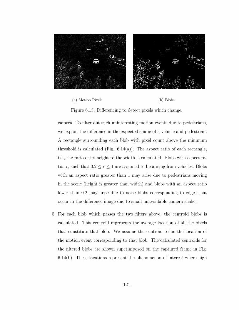
(a) Motion Pixels (b) Blobs
Figure 6.13: Differencing to detect pixels which change.
camera. To filter out such uninteresting motion events due to pedestrians,
we exploit the difference in the expected shape of a vehicle and pedestrian.
A rectangle surrounding each blob with pixel count above the minimum
threshold is calculated (Fig. 6.14(a)). The aspect ratio of each rectangle,
i.e., the ratio of its height to the width is calculated. Blobs with aspect ra-
tio, r, such that 0.2 ≤ r ≤ 1 are assumed to be arising from vehicles. Blobs
with an aspect ratio greater than 1 may arise due to pedestrians moving
in the scene (height is greater than width) and blobs with an aspect ratio
lower than 0.2 may arise due to noise blobs corresponding to edges that
occur in the difference image due to small unavoidable camera shake.
5. For each blob which passes the two filters above, the centroid blobs is
calculated. This centroid represents the average location of all the pixels
that constitute that blob. We assume the centroid to be the location of
the motion event corresponding to that blob. The calculated centroids for
the filtered blobs are shown superimposed on the captured frame in Fig.
6.14(b). These locations represent the phenomenon of interest where high
121

resolution coverage is desired.
(a) Aspect Ratio (b) Filtered Events
Figure 6.14: Filtering motion events of interest for phenomenon detection.
The above procedures yields the location of the events in the image pixel
coordinates. This is sufficient for controlling the actuation when only a camera
which detects a phenomenon in its field of view must actuate to it since then, the
camera can direct its actuation based on its its own pixel coordinates. However,
if a camera other than the one used for detection must be used for the actu-
ation step, more detailed information about the event coordinates in the three
dimensional space may be required.
For our scenario for the latter application of imaging vehicles, where the plane
of the road is known, the image coordinate may be projected to the road surface
using geometric calculations. This may not be feasible in some applications and
the true coordinates of the events in 3-space may be needed. More sophisticated
detection methods, such as triangulation of the detected phenomenon’s location
by having it imaged via two or more cameras, may be studied for that objective.
In this chapter we have described the supporting services relevant for our mo-
tion coordination algorithm. Next, we consider the simulations and experiments
122

performed to evaluate our proposed methods and demonstrate their operation on
a real system.
123
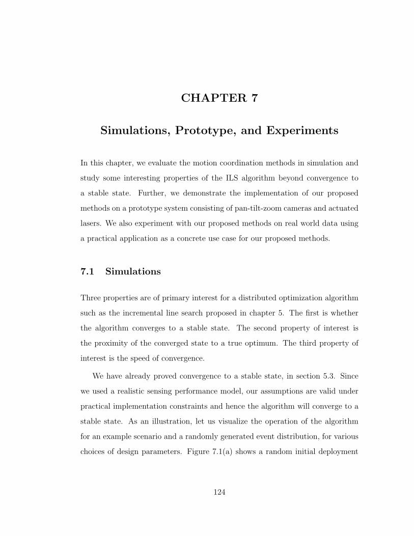
CHAPTER 7
Simulations, Prototype, and Experiments
In this chapter, we evaluate the motion coordination methods in simulation and
study some interesting properties of the ILS algorithm beyond convergence to
a stable state. Further, we demonstrate the implementation of our proposed
methods on a prototype system consisting of pan-tilt-zoom cameras and actuated
lasers. We also experiment with our proposed methods on real world data using
a practical application as a concrete use case for our proposed methods.
7.1 Simulations
Three properties are of primary interest for a distributed optimization algorithm
such as the incremental line search proposed in chapter 5. The first is whether
the algorithm converges to a stable state. The second property of interest is
the proximity of the converged state to a true optimum. The third property of
interest is the speed of convergence.
We have already proved convergence to a stable state, in section 5.3. Since
we used a realistic sensing performance model, our assumptions are valid under
practical implementation constraints and hence the algorithm will converge to a
stable state. As an illustration, let us visualize the operation of the algorithm
for an example scenario and a randomly generated event distribution, for various
choices of design parameters. Figure 7.1(a) shows a random initial deployment
124
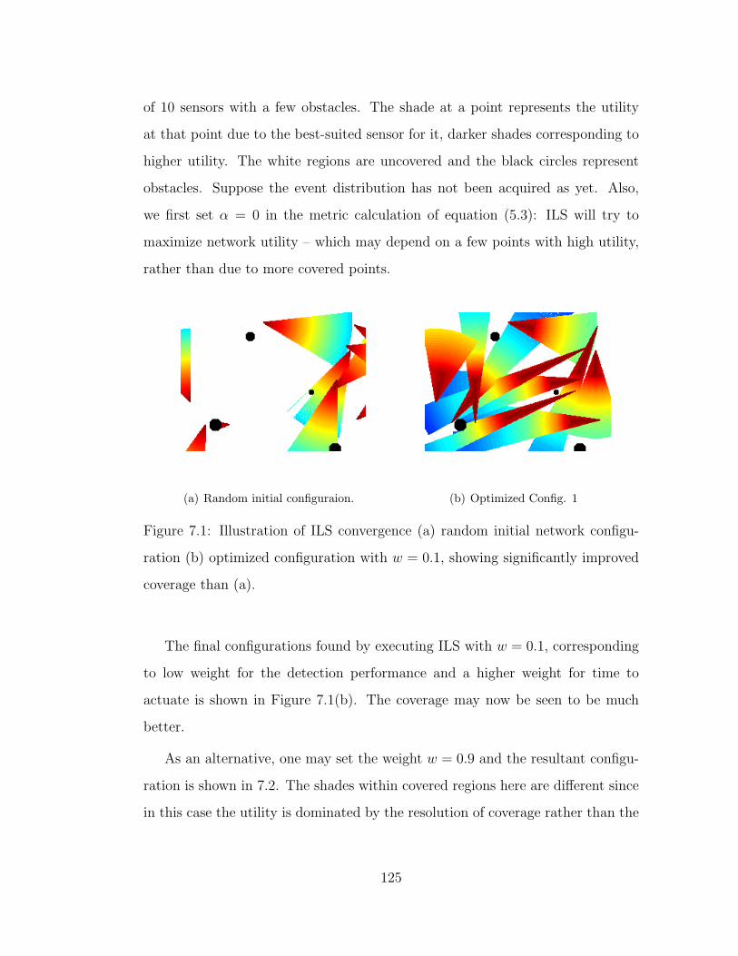
of 10 sensors with a few obstacles. The shade at a point represents the utility
at that point due to the best-suited sensor for it, darker shades corresponding to
higher utility. The white regions are uncovered and the black circles represent
obstacles. Suppose the event distribution has not been acquired as yet. Also,
we first set α = 0 in the metric calculation of equation (5.3): ILS will try to
maximize network utility – which may depend on a few points with high utility,
rather than due to more covered points.
(a) Random initial configuraion. (b) Optimized Config. 1
Figure 7.1: Illustration of ILS convergence (a) random initial network configu-
ration (b) optimized configuration with w = 0.1, showing significantly improved
coverage than (a).
The final configurations found by executing ILS with w = 0.1, corresponding
to low weight for the detection performance and a higher weight for time to
actuate is shown in Figure 7.1(b). The coverage may now be seen to be much
better.
As an alternative, one may set the weight w = 0.9 and the resultant configu-
ration is shown in 7.2. The shades within covered regions here are different since
in this case the utility is dominated by the resolution of coverage rather than the
125

time to actuate. The exact choice of the weight parameter depends on desired
behavior, which is application specific and we do not dwell on it further here.
Figure 7.2: Illustration of ILS: optimized coverage using w = 0.9, showing a
different stable state.
Suppose next that the event distribution shown in Figure 7.3(a) is acquired.
The figure axes represent the spatial extent and the shade at each location corre-
sponds to the event density at that location. In the simulation this event distri-
bution is generated as a sum of two Gaussian distributions. The ILS algorithm
can use this distribution in the calculation of its utility metric. The optimized
configuration is shown in Figure 7.3(b) with w = 0.1 - the prominence of higher
zoom (narrower field of view) in the diagonal region with higher event density
is apparent. Suppose however that the area covered is also to be kept high and
thus α is set to 0.8. This yields the configuration in Figure 7.3(c).
The above illustration shows how the ILS algorithm can be tuned for different
behaviors as desired by the user application.
We now discuss the other two properties of interest in simulations.
126

(a) Sample Event Distribution
(b) Optimized Config. 3 (c) Optimized Config. 4
Figure 7.3: Illustration of ILS (a) a sample event distribution, where brighter
areas show higher event density (b) optimized configuration after learning the
event distribution, and (c) optimized configuration with α set to a high value.
7.1.1 Accuracy of Converged State
As was proved in section 5.2.1, the optimization problem being solved is NP-
hard and our proposed algorithm is a computationally tractable heuristic to solve
it, with certain desirable characteristics such as its distributed nature. It may
127
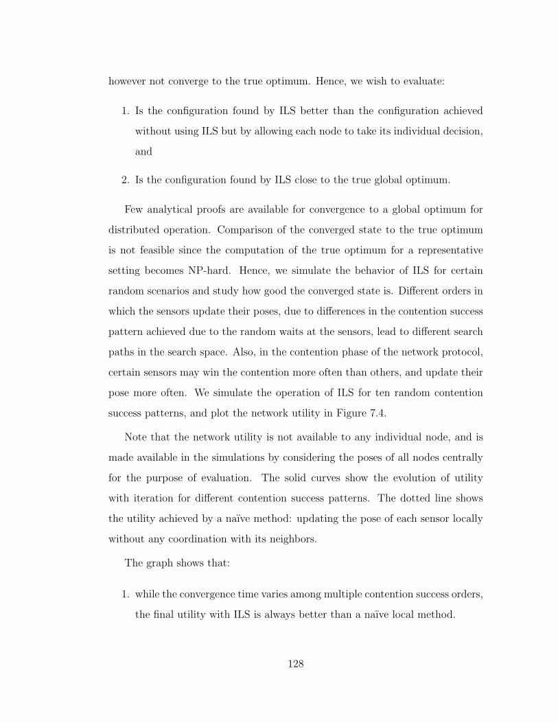
however not converge to the true optimum. Hence, we wish to evaluate:
1. Is the configuration found by ILS better than the configuration achieved
without using ILS but by allowing each node to take its individual decision,
and
2. Is the configuration found by ILS close to the true global optimum.
Few analytical proofs are available for convergence to a global optimum for
distributed operation. Comparison of the converged state to the true optimum
is not feasible since the computation of the true optimum for a representative
setting becomes NP-hard. Hence, we simulate the behavior of ILS for certain
random scenarios and study how good the converged state is. Different orders in
which the sensors update their poses, due to differences in the contention success
pattern achieved due to the random waits at the sensors, lead to different search
paths in the search space. Also, in the contention phase of the network protocol,
certain sensors may win the contention more often than others, and update their
pose more often. We simulate the operation of ILS for ten random contention
success patterns, and plot the network utility in Figure 7.4.
Note that the network utility is not available to any individual node, and is
made available in the simulations by considering the poses of all nodes centrally
for the purpose of evaluation. The solid curves show the evolution of utility
with iteration for different contention success patterns. The dotted line shows
the utility achieved by a naıve method: updating the pose of each sensor locally
without any coordination with its neighbors.
The graph shows that:
1. while the convergence time varies among multiple contention success orders,
the final utility with ILS is always better than a naıve local method.
128
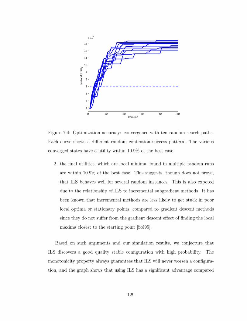
0 10 20 30 40 50
4
5
6
7
8
9
10
11
12
13
x 104
Iteration
Net
wor
k U
tility
Figure 7.4: Optimization accuracy: convergence with ten random search paths.
Each curve shows a different random contention success pattern. The various
converged states have a utility within 10.9% of the best case.
2. the final utilities, which are local minima, found in multiple random runs
are within 10.9% of the best case. This suggests, though does not prove,
that ILS behaves well for several random instances. This is also expeted
due to the relationship of ILS to incremental subgradient methods. It has
been known that incremental methods are less likely to get stuck in poor
local optima or stationary points, compared to gradient descent methods
since they do not suffer from the gradient descent effect of finding the local
maxima closest to the starting point [Sol95].
Based on such arguments and our simulation results, we conjecture that
ILS discovers a good quality stable configuration with high probability. The
monotonicity property always guarantees that ILS will never worsen a configura-
tion, and the graph shows that using ILS has a significant advantage compared
129
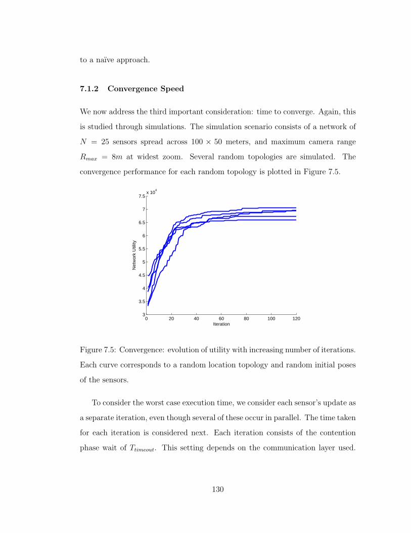
to a naıve approach.
7.1.2 Convergence Speed
We now address the third important consideration: time to converge. Again, this
is studied through simulations. The simulation scenario consists of a network of
N = 25 sensors spread across 100 × 50 meters, and maximum camera range
Rmax = 8m at widest zoom. Several random topologies are simulated. The
convergence performance for each random topology is plotted in Figure 7.5.
0 20 40 60 80 100 1203
3.5
4
4.5
5
5.5
6
6.5
7
7.5x 10
4
Iteration
Net
wor
k U
tility
Figure 7.5: Convergence: evolution of utility with increasing number of iterations.
Each curve corresponds to a random location topology and random initial poses
of the sensors.
To consider the worst case execution time, we consider each sensor’s update as
a separate iteration, even though several of these occur in parallel. The time taken
for each iteration is considered next. Each iteration consists of the contention
phase wait of Ttimeout. This setting depends on the communication layer used.
130

For instance, for 802.11 MAC, the per hop delay is expected to be less than 10ms
[TS04, GK04] and, if γi spans 10 hops as a worst case estimate, the total round
trip delay would be limited to 200ms. At least one sensor wins the contention
and computes its optimal pose. This has the delay of pan motion and zoom
motion. The longest pan step may be 340◦ degrees which takes 2 seconds. The
longest zoom step (see Figure 3.14-(b)) allowing a maximum zoom setting of 5 in
detection mode (leaving the remaining zoom range of 20 available for providing
high resolution coverage for recognition), is 1.3s. A single update time is thus
2 + 1.3 + 0.2 = 3.5s.
The number of iterations required to achieve the final utility is about 80 as seen
in the graph for each random topology, and even in the worst case this requires
4 minutes 40 seconds. The number of iterations is about 3 times the number of
sensors, implying that on an average each sensor updates three times. Even with
increasing network size, due to parallelism in updates, the convergence time will
stay at the same order. Thus the stable state is discovered in only a few minutes
for the hardware capabilities in our system. Since the phenomenon learning phase
(which must wait for several events to occur in order to estimate or update the
q(p)) and medium dynamics are expected to be much slower, convergence time is
not an important consideration for our system, and ILS can repeatedly be used
to update the network configuration whenever new environmental information
becomes available.
Time to converge may be an important concern in other applications of ILS
where the system must deal with rapid dynamics. The graceful degradation
behavior of ILS discussed in section 5.3.1 then helps ensure that ILS does not
worsen the situation.
131

7.2 Prototype System
Let us now consider the execution of ILS on the test-bed shown in Figure 1.2. The
test-bed has four pan-tilt-zoom cameras [Son04]. The motion capabilities of this
camera have already been tabulated (Table 3.2). It also has two self-awareness
nodes described in section 6.1.1.1. Some objects of various shapes are placed
to emulate obstacles in the covered space. Any available networking technology
that has sufficient bandwidth to support video data, may be used and we used
Ethernet. The cameras also allow for a WiFi card to be added in its PCMCIA
slot and that may be used if a wireless connection is preferred. Since we did not
have access to change the firmware on the camera, we developed our software on
an external processing platform but the methods could well be implemented on
the camera processor itself in actual production.
Rather than beginning with a random configuration, we arrange the cameras
along the edges to form a regular tessellation covering the entire rectangular
region of interest. However, the obstacles in the rectangular region, render the
regular tessellation ineffective.
The first requirement is the information about medium obstacles. We collect
this using laser ranging. Range scans from the bottom left corner and the top
right are shown in Figures 7.6(a) and 7.6(b) repectively. Note that these scans
exploit the adaptive scanning enhancements discussed in section 6.1 and hence
the scan step size is seen to be greater when scanning a structured environmental
feature, such as a straight line, since it matches the adaptive algorithm’s predicted
structure. A backtracking procedure allows the algorithm to reduce the scan step
size and re-scan the missed portion in case a large deviation from the predicted
structure is observed. Combining the two scans yields the obstacle map shown
in Figure 7.6(c) by the dark patches. Figure 7.6(c) also shows the initial network
132

configuration.
0 0.5 1 1.5 2 2.50
0.5
1
1.5
2
(a) Range scan 1
0 0.5 1 1.5 2 2.50
0.5
1
1.5
2
(b) Range scan 2
(c) Obstacles and Initial Configuration (d) Final configuration
Figure 7.6: Gathering medium information for ILS operation (a) range scan
from laser in bottom left corner (b) range scan from laser in top right corner,
(c) map of obstacles in the medium and the initial network configuration, (d)
optimized configuration found by ILS - it changes both the pan and zoom settings
of the cameras to increase sensing performance characterized by time required for
recognition.
In this configuration, each sensor node has all other nodes as its neighbors.
The test-bed can thus be viewed as one neighborhood set in a larger network.
133

The final network configuration found by the ILS algorithm is shown in Figure
7.6(d). The experiment used w = 0.1, thus giving more weight to the time
required for actuation and the parameter α was set high to maximize covered
area. These results not only verified that the ILS algorithm behaves as designed
but also helped us ensure that all the algorithms and methods proposed can be
implemented in a real system.
The testbed software also includes certain supporting components to enable
visualization of the experiment’s progress. The images captured by the network
cameras are compressed JPEG files for ease of transfer over the network. Our
camera controller software decompresses each image. It also calculates the oc-
cluded pixels based on the laser ranger readings. The occluded pixels are plotted
superimposed on the raw image for visualizing the camera’s field of view as it
evolves under ILS. A snapshot of the visualization of four separate processes,
each controlling one of the network cameras is shown in Figure 7.7.
A central experiment monitoring program was also developed in Matlab for
controlling the cameras centrally for various experiments. The graphical user
interface to this program alows setting various parameters in the experiment,
and is shown in Figure 7.8.
Further, a manual control interface was developed which exposed the camera’s
actuation capabilities to a human user through an HTML interface. This manual
control interface allows a user to manually over-ride the settings found by ILS
if so desired. The complete system software in operation, including the manual
over-ride may be seen in Figure 7.9.
134
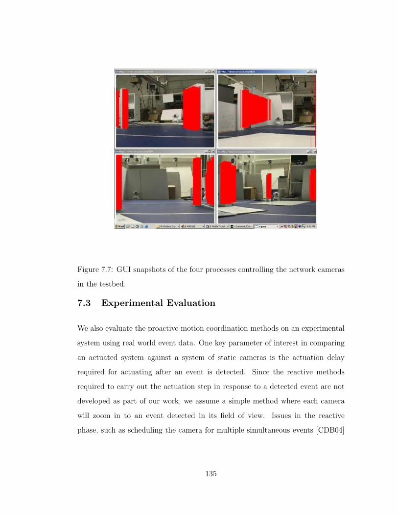
Figure 7.7: GUI snapshots of the four processes controlling the network cameras
in the testbed.
7.3 Experimental Evaluation
We also evaluate the proactive motion coordination methods on an experimental
system using real world event data. One key parameter of interest in comparing
an actuated system against a system of static cameras is the actuation delay
required for actuating after an event is detected. Since the reactive methods
required to carry out the actuation step in response to a detected event are not
developed as part of our work, we assume a simple method where each camera
will zoom in to an event detected in its field of view. Issues in the reactive
phase, such as scheduling the camera for multiple simultaneous events [CDB04]
135

Figure 7.8: Experiment monitoring software.
or tracking an event as it moves through the covered area [CRZ04, CLF01] are
not being studied here.
While most of our design choices apply generically to any camera network
where resolution is to be increased, some of the analysis is performed in the
context of the example application mentioned briefly in section 1, and specified
concretely here. Consider the access road to a building shown in Fig. 1.1(a). This
image is captured from a camera mounted on a 2nd floor patio of the building
itself. Suppose the entire sealed road area in this scene is to be photographed at
a resolution good enough to visually recognize a vehicle, say 200pixels/m. The
vehicle license plate, if captured in the image, will be legible at this resolution.
However, cameras may be installed only within the building premises and not on
136

Figure 7.9: System software in operation alongside the testbed.
the roads themselves since the building owners may not have jurisdiction over the
road infrastructure or the sidewalks. Given that the application is interested in
photographing vehicles, assuming that the minimum vehicle width is 1.5m, and
also assuming that motion detection can work reliably if the one of the moving
object dimensions is at least 15 pixels, we see that Rdet = 10pixels/m. For the
required Rsense = 200pixels/m, this yields z = 20X. The camera we use in our
system [Son04] has a zoom range, zhw, greater than this. The range of pan and
tilt required, for the reactive actuation when an event is detected, is equal to the
angle of field of view at the zoom setting used for detection. For instance, the
angle of field of view is 45◦ at the widest zoom setting, z = 1, and the pan range
of the camera is greater than this. The available actuation capabilities of the
137

camera are compared to those required in Table 7.1.
Capability Required Available
Zoom z=20X zhw = 25X
Pan θfov = 45◦ θpan = 370◦
Tilt 30◦ 115◦
Table 7.1: Required actuation ranges and hardware capabilities.
We will compare the network configurations achieved by our method and
other methods by measuring the actuation delay per event averaged over a large
number of events.
To obtain a realistic trace of event locations in the covered area of interest, we
used motion detection, as described in section 6.2.3, on a live stream of images
coming from a camera mounted to view the scene shown in Fig. 1.1(a). Note
that we are not addressing the problem of detection method design in this thesis
and assume that the detection performance achieved by the available method,
such as motion detection in our example, is sufficient for system operation.
A total of 5000 events were detected using the above procedure in a live
video stream. A histogram of these events over the scene coordinates is shown
in Fig.7.10. Lighter shades correspond to regions with more events. The com-
plete image stream, and the event coordinates obtained via motion detection are
available through our CVS repository [Kan].
The proactive motion coordination methods are evaluated using this event
trace for a set up of four cameras looking at the scene for which this event trace is
collected. The actuation delay performance of a particular network configuration
is calculated as follows: for each event in the trace, the time required by the
camera to zoom in to provide the high resolution coverage is computed. The
138

Figure 7.10: Event trace
time is computed for that camera which has detection coverage (low resolution
coverage) over the event location. This time varies with the extent of zoom,
pan, and tilt motion required to reach that event, and can be computed using
the documented pan and tilt speeds for the camera along with the measured
zoom change speed of the camera (Figure 3.14(b)). An average of the computed
time for each event is taken over all events, for each configuration as the delay
performance of that configuration.
We compare four alternatives, labeled in the following graphs using the acronyms
below:
1. TESS, a regular tessellation: The four cameras are arranged regularly with
their zoom set to widest and each camera looking straight ahead.
2. ILS(UNIF): The ILS algorithm is used to optimize the configuration. Only
139

5X of the zoom is used since the remaining 20X is required for the reactive
phase. Similarly, the excess pan range not required for the reactive phase
is used. The tilt is ignored, but can be used in the same manner as pan.
3. ILS: The ILS algorithm is used with a knowledge of the true event distrib-
ution. The histogram generated from the event trace is used as the event
distribution, and since this comes from the trace itself, it is a true event
distribution. If the observed event distribution varies from the distribution
learned by the system, the delay performance may suffer somewhat; the
exact deviation depends on the error in the learned distribution itself.
4. RAND: The cameras are configured randomly. Ten random configurations
are tried and the average and standard deviation of the quantities being
evaluated are plotted.
In the utility metric used for ILS, the tuning parameter w allows biasing
the algorithm toward actuation delay or detection quality. Suppose we bias it to
actuation delay, by using a higher weight w = 0.9 for the delay term and (1−w) =
0.1 for the detection term. The delay performance for the four alternatives is
plotted in Fig. 7.11(a). The corresponding detection performance, measured in
terms of the fraction of the events detected is plotted in Figure 7.11(b). The
lighter shade bar segment on top of the bar for RAND is the standard deviation
across the multiple random runs. Clearly ILS yields the best delay performance.
The detection performance is comparable, though not exactly the same, for all
alternatives except RAND. It is above 90%, showing that when ILS optimizes
for delay, the penalty on detection is not significant. For applications where the
detection performance is at a premium, delay may have to be sacrificed by chosing
the configuration with the highest detection performance.
140

TESS ILS(UNIF) ILS RAND0
0.1
0.2
0.3
0.4
0.5
0.6
0.7
0.8
0.9
Del
ay (
s)
(a) Actuation delay
TESS ILS(UNIF) ILS RAND0
50
100
Cov
erag
e (%
)
(b) Detection coverage
Figure 7.11: Performance of different network configurations, when optimization
is weighted for actuation delay.
Note that internally, the ILS algorithm is not using delay but the utility metric
defined in section 5.1.3 for optimizing the configuration. This utility metric for
the four alternatives is plotted in Fig. 7.12, to see how this internal measure
relates to the observed application level performance metrics. The configurations
obtained using ILS have higher utility. This is expected as the ILS algorithm
changes the starting configuration to increase the utility metric. Among these,
the utility is higher when the true event distribution is used.
141

TESS ILS(UNIF) ILS RAND0
0.5
1
1.5
2
2.5x 10
5
Util
ity
Figure 7.12: Utility metric evaluated for various configurations.
On the other hand, we could bias the utility metric for detection performance,
using the tuning parameter w provided by our algorithm. The results for this
choice, i.e., the weight for delay term set to w = 0.1, and that for detection
term set to (1 − w) = 0.9, are shown in Figs. 7.13 and 7.14. As may be seen
in Fig. 7.13(b), the detection performance has improved. Since the detection
performance was already high, the improvement relative to Fig. 7.11(b) is small.
The above evaluations show the delay required using our prototype hardware
to increase the resolution of sensing by over an order of magnitude. Clearly,
when such delay is acceptable, our methods can be used to improve the sensing
performance significantly, or conversely, to provide significant savings in sensing
resources for a given sensing performance. Further, the graphs above indicate the
flexibility of our algorithm provided through the tuning parameters for biasing
142

TESS ILS(UNIF) ILS RAND0
0.1
0.2
0.3
0.4
0.5
0.6
0.7
0.8
Del
ay (
s)
(a) Actuation delay
TESS ILS(UNIF) ILS RAND0
50
100
Cov
erag
e (%
)
(b) Detection coverage
Figure 7.13: Performance of different network configurations, when configuration
optimization is weighted for detection performance.
its operation for the metric of user interest.
The delay can be further reduced by increasing the number of cameras. For
instance, if each camera in our system is replaced with 4 similar cameras, then
each camera is responsible for only a quarter of the original volume covered for
detection and a lower actuation time is sufficient to cover the reduced volume.
In our prototype, we use four cameras based on equipment availability. In actual
143

TESS ILS(UNIF) ILS RAND0
0.5
1
1.5
2
2.5x 10
5
Util
ity
Figure 7.14: Utility metric for various configurations, when detection performance
is weighted higher.
production, the number of cameras may be determined based on the desired delay
tolerance and the expected number of simultaneous events in the scene.
144

CHAPTER 8
Conclusions and Future Work
In this dissertation we discussed why using small motion is a potentially useful
alternative to improve the sensing performance of embedded sensor networks
and provided a framework of distributed methods to effectively exploit the small
motion.
While it has been known before that motion and even small motion has a
sensing advantage, a quantitative understanding of the potential benefits and an
in-depth analysis of the related trade-offs was lacking. Our work has evaluated the
exact extent of sensing advantage that may be achieved using small motion and
also compared it to other alternatives such as using a high density of static sensors
or a low density of unconstrained mobile nodes. We showed that small motion can
lead to several orders of magnitude advantage in sensing resolution depending on
certain trade-offs and in our particular prototype, we demonstrated four orders of
magnitude advantage. We also discussed several reasons which make the use of
small or constrained motion more practical than other alternatives for a variety
of scenarios.
Further, while motion has been used before for increasing the range of coverage
or for tracking mobile phenomenon before, the precise delay trade-off in the use of
motion had not been discussed. We quantified the delay trade-off in using small
motion for providing high resolution coverage for a specific methodology of using
motion: using a low resolution view for detecting the phenomenon of interest and
145

then using motion to provide high resolution sensing at required locations.
We also presented a framework for optimizing the configuration of a mobile
sensor network with limited motion capabilities. Prior work has considered the
use of motion for optimizing the deployment in terms of area covered, increasing
the extent of coverage by having a sensor patrol a set of sensing points, or even
the use of motion to track a mobile phenomenon. However, the use of motion to
increase the resolution of coverage by using a low resolution view for detection
has not been studied in depth before. Using motion for configuring the network
in order to minimize motion delay had not been considered in prior work. We
provided methods that allow minimizing the motion delay required for providing
high resolution coverage. We showed that solving this problem optimally was NP-
hard and provided computationally tractable heuristics to address the situation.
The motion coordination methods we developed for the above objective were
distributed in nature. This leads to extreme scalability of the proposed methods
in terms of the number of nodes in the network since the motion coordination
algorithm required communication only in a well defined neighborhood, the size
of which depends only on the network density and does not grow with the num-
ber of nodes. The distributed motion coordination algorithm developed as part
of this work was shown to have several desirable properties, including provable
convergence, graceful degradation and the ability to operate with realistic sensor
models.
In addition to the motion coordination method, we also presented practical
methods to learn the environmental parameters which affect the network configu-
ration. Specifically, our methods could exploit information about the obstacles in
the medium and the expected distribution of events in the space covered. Prac-
tical methods for acquiring this information about the environment were also
146
developed and demonstrated with prototype hardware implementations.
Finally, we implemented all our proposed methods on a prototype system to
not only verify their realizability but also study their behavior with respect to
certain performance considerations. We also conducted experiments to evaluate
our methods on real world data collected using our prototype in the context of
practical application examples.
8.1 Future Directions
Most of the methods developed as part of our work are the first in the domain
of minimizing actuation delay in using motion for high resolution sensing. Thus,
significant future research is feasible to improve the proposals of our work.
An interesting problem for future research is the integration of the proac-
tive methods for network reconfiguration presented in our work with the reactive
methods used to perform the final actuation in response to detected events. The
network configuration provided by our proactive methods can be exploited by the
reactive methods to achieve the best delay performance in the face of multiple
events detected by multiple sensors. The scheduling of actuation steps and the
allocation of appropriate sensing resources to the detected events presents inter-
esting research challenges. For instance, methods may be developed to prioritize
the detected events based on their dwell time in the field of view of the network,
and then use the allocating the cameras in the derived priority order to those
events.
Future work also includes fundamental considerations that relate the number
of actuated cameras required for given event dynamics in terms of the number
of events in the environment and their dwell times and mobility characteristics.
147

The appropriate strategy to use all available sensors for detection and actuation
for high resolution sensing on demand, or allocating a fixed number of sensors for
constant detection while others are used for actuation may be studied as part of
this problem as well.
The ILS algorithm may further be extended to exploit the temporal dimension
and determine sequences of configurations to be visited over a given time period
rather than finding a single optimal configuration. Further, our methods may be
extended to include the case of tracking mobile events rather than just providing
high resolution coverage once for each event.
148
References
[AB03] MD Naish A Bakhtari, M Eskandari and B Benhabib. “A Multi-Sensor Surveillance System for Active-Vision Based Object Localiza-tion.” In IEEE International Conference on Systems, Man and Cy-bernetics, volume 1, p. 10131018, Washington, D.C., October 2003.
[AKS03] A Antoniades, HJ Kim, and S Sastry. “Pursuit-evasion strategies forteams of multiple agents with incomplete information.” In 42nd IEEEConference on Decision and Control, Maui, Hawaii, USA, December2003.
[AMB05] S Aranda, S Martinez, and F Bullo. “On optimal sensor placementand motion coordination for target tracking.” In IEEE Int. Conf. onRobotics and Automation, Barcelona, Spain, April 2005.
[AMN95] AS Aguado, ME Montiel, and MS Nixon. “Ellipse Detection via gra-dient direction in the Hough transform.” In Proc. IEE InternationalConference on Image Processing and its Applications, pp. 375–378,July 1995.
[APP02] T Arai, E Pagello, and LE Parker. “Editorial: advances in Multi-Robot Systems.” IEEE Transactions on Robotics and automation,18(5):655–661, October 2002.
[AXI] AXIS. “Axis 2100 Network Camera.”Product Datasheet, Axis Communications,http://www.axis.com/documentation/datasheet/2100/2100 ds.pdf.
[BC04] G Biegel and V Cahill. “A Framework for Developing Mobile,Context-aware Applications.” In IEEE Percom, Orlando, FL, March2004.
[BMK02] J Burke, E Mendelowitz, J Kim, and R Lorenzo. “Networking withknobs and knats: Towards ubiquitous computing for artists.” InUbiquitous Computing, Concepts and Models Workshop, Gothenburg,Sweden, 2002.
[BP98] I Benyahia and JY Potvin. “Decision Support for Vehicle DispatchingUsing Genetic Programming.” IEEE Transations on Systems, Man,and CyberneticsPart A: Systems and Humans, 28(3), May 1998.
149

[BR03] Z Butler and D Rus. “Event-Based Motion Control for Mobile-Sensor Networks.” IEEE Pervasive Computing, 2(4):34–42, October-December 2003.
[BRD05] NP Bichot, AF Rossi, and R Desimone. “Parallel and Serial NeuralMechanisms for Visual Search in Macaque Area V4.” Science,308(5721):529–534, April 2005.
[BRY04] M Batalin, M Rahimi, Yan Yu, Duo Liu, A Kansal, G Sukhatme,WJ Kaiser, M Hansen, GJ Pottie, and D Estrin. “Call and Response:Experiments in Sampling the Environment.” In ACM SenSys, No-vember 2004.
[BSP04] B Batagelj, F Solina, and P Peer. “15 seconds of fame - an inter-active, computer-vision based art installation.” In Proceedings of the12th ACM International Conference on Multimedia, pp. 764–765, NewYork, NY, USA, October 2004.
[CD00] X Chen and J Davis. “Camera Placement Considering Occlusions forRobust Motion Capture.” Technical Report CS-TR-2000-07, Com-puter Science, Stanford University, 2000.
[CDB04] C Costello, C Diehl, A Banerjee, and H Fisher. “Scheduling an ActiveCamera to Observe People.” In ACM 2nd International Workshop onVideo Surveillance and Sensor Networks, New York City, NY, USA,October 2004.
[CEE01] A Cerpa, J Elson, D Estrin, L Girod, M Hamilton, and J Zhao. “Habi-tat monitoring: Application driver for wireless communications tech-nology.” In ACM SIGCOMM Workshop on Data Communications inLatin America and the Caribbean, 2001.
[Cho] Howie Choset. “The Wide World of Mapping.” WTEC Workshop:Review of US Research in Robotics.
[Chv75] V Chvatal. “A Combinatorial theorem in plane geometry.” Journalof Combinatorial Theory Series, 18:39–41, 1975.
[CK00] G Chen and D Kotz. “A Survey of Context-Aware Mobile Comput-ing Research.” Technical Report TR2000-381, Dept. of ComputerScience, Dartmouth College, November 2000.
150

[CL04] Z Cheng and Y Liu. “Efficient Technique for Ellipse Detection UsingRestricted Randomized Hough Transform.” In International Confer-ence on Information Technology: Coding and Computing (ITCC’04),volume 2, p. 714, 2004.
[CLF01] R Collins, A Lipton, H Fujiyoshi, and T Kanade. “Algorithmsfor cooperative multisensor surveillance.” Proceedings of the IEEE,89(10):1456 – 1477, October 2001.
[CMB04] J Cortes, S Martinez, and F Bullo. “Spatially-distributed coverageoptimization and control with limited range interactions.” ESAIM,Control, Optimization and Calculus of Variations, January 2004.
[CMB05] J Cortes, S Martinez, and F Bullo. “Analysis and design tools fordistributed motion coordination.” In American Control Conference,Portland, OR, June 2005.
[CN88] W P Chin and S Ntafos. “Optimum watchman routes.” InformationProcessing Letters, 28:3944, 1988.
[CNN93] S Carlsson, BJ Nilsson, and SC Ntafos. “Optimum Guard Covers andm-Watchmen Routes for Restricted Polygons.” International Journalof Computational Geometry Applications, 3(1):85–105, 1993.
[CRZ04] M Chu, J Reich, and F Zhao. “Distributed Attention for Large VideoSensor Networks.” In Intelligent Distributed Surveillance Systems2004 seminar, London, UK, February 2004.
[DNC01] MWM Gamini Dissanayake, P Newman, S Clark, HF Durrant-Whyte,and M Csorba. “A Solution to the Simultaneous Localization andMapping (SLAM) Problem.” IEEE Transactions on Robotics andAutomation, 17(3):229–241, June 2001.
[Dpe] “Directed Perception.” http://www.dperception.com.
[DR04] D Devarajan and R Radke. “Distributed metric calibration forlargescale camera networks.” In First Workshop on Broadband Ad-vanced Sensor Networks (BASENETS), in conjunction with Broad-Nets, San Jose, October 2004.
[EAB92] T Ellis, A Abbood, and B Brillault. “Ellipse Detection and Match-ing with Uncertainty.” Image and Vision Computing, 10(5):271–276,June 1992.
151
[EGH00a] A Efrat, LJ Guibas, S Har-Peled, DC Lin, JSB Mitchell, and TM Mu-rali. “Sweeping simple polygons with a chain of guards.” In SODA’00: Proceedings of the eleventh annual ACM-SIAM symposium onDiscrete algorithms, pp. 927–936, San Francisco, California, UnitedStates, 2000.
[EGH00b] D Estrin, R Govindan, and J Heidemann. “Embedding the Internet:introduction.” Communications of the ACM, 43(5):38–41, 2000.
[ES04] UM Erdem and S Sclaroff. “Optimal Placement of Cameras in Floor-plans to Satisfy Task Requirements and Cost Constraints.” In Om-nivis2004, The fifth Workshop on Omnidirectional Vision, CameraNetworks and Non-classical cameras, Prague, May 2004.
[Far01] CR Farrar. Lecture notes on Structural Health Monitoring using Sta-tistical Pattern Recognition, chapter Historical overview of structuralhealth monitoring. Los Alamos Dynamics, Los Alamos, NM, 2001.
[FGP06] S Funiak, C Guestrin, M Paskin, and R Sukthankar. “DistributedLocalization of Networked Cameras.” In Inormation Processing inSensor Networks, Nashville, TN, USA, April 2006.
[Fis78] S Fisk. “A short proof of Chvatal’s watchmen theorem.” Journal ofCombinatorial Theory Series, 24:374, 1978.
[FLS02] JT Feddema, C Lewis, and DA Schoenwald. “Decentralized Controlof Cooperative Robotic Vehicles: Theory and Application.” IEEETransactions on Robotics and Automation, 18(5), October 2002.
[GA81] H. El Gindy and D Avis. “A linear algorithm for computing thevisibility polygon from a point.” Journal of Algorithms, 2:186–197,1981.
[GJ96] D Geman and B Jedynak. “An Active Testing Model for TrackingRoads in Satellite Images.” IEEE Trans. Pattern Anal. Mach. Intell.,18(1):1–14, 1996.
[GK04] N Gupta and PR Kumar. “A Performance Analysisof the 802.11 Wireless LAN Medium Access Control.”http://www.ece.rice.edu/camp/MAC/MAC Analysis.pdf, 2004.Submitted to Communications in Information and Systems , Jan’04,revised June’04.
152

[GKS04] S Ganeriwal, A Kansal, and MB Srivastava. “Self-aware Actuation forFault Repair in Sensor Networks.” In IEEE International Conferenceon Robotics and Automation (ICRA), April 2004.
[GLL99] LJ Guibas, JC Latombe, SM LaValle, D Lin, and R Motwani. “Avisibility-based pursuit-evasion problem.” International Journal ofComputational Geometry and Applications, 9(4/5):471–, 1999.
[GMK03] B Grocholsky, A Makarenko, T Kaupp, and HF Durrant-Whyte.“Scalable Control of Decentralised Sensor Platforms.” In Informa-tion Processing in Sensor Networks: 2nd Int Workshop, IPSN03, pp.96–112, 2003.
[GP04] V Gazi and KM Passino. “Stability Analysis of Social ForagingSwarms.” IEEE Transactions on Systems, Man, and CyberneticsPartB: Cybernetics, 34(1), February 2004.
[Gro02] B Grochoslsky. Information Theoretic Control of Multiple SensorPlatforms. PhD thesis, Australian Center for Field Robotics, Depart-ment of Aerospace, Mechatronic and Mechanical Engineering, Uni-versity of Sydney, March 2002.
[HAG06] TC Harmon, RF Ambrose, RM Gilbert, JC Fisher, M Stealey, andWJ Kaiser. “High Resolution River Hydraulic and Water QualityCharacterization Using Rapidly Deployable Networked Infomechani-cal Systems (NIMS RD).” Technical Report 60, Center for EmbeddedNetworked Sensing, University of California Los Angeles, February 302006.
[Hay01] S Haykin. Adaptive Filter Theory. Prentice Hall, 4th edition, 2001.
[HH03] RK Harle and A Hopper. “Building World Models by Ray Tracingwithin Ceiling Mounted Positioning Systems.” In UbiComp 2003, pp.1–17, Seattle, WA, USA, October 2003.
[HMS02a] A Howard, MJ Mataric, and GS Sukhatme. “An Incremental Self-Deployment Algorithm for Mobile Sensor Networks.” AutonomousRobots Journal (Special Issue on Intelligent Embedded Systems),13(2):113–126, 2002.
[HMS02b] A Howard, MJ Mataric, and GS Sukhatme. “An Incremental Self-Deployment Algorithm for Mobile Sensor Networks.” AutonomousRobots Journal (Special Issue on Intelligent Embedded Systems),13(2):113–126, 2002.
153

[HS97] J Heikkila and O Silven. “A Four Step Camera Callibration Proce-dure with Implicit Image Correction.” In IEEE Computer Vision andPattern Recognition, pp. 1106–1112, 1997.
[IL01] D Lpez de Ipia and SL Lo. “Video-Based Sensing for Wide Deploy-ment of Sentient Spaces ’’ In 2nd PACT Workshop on UbiquitousComputing and Communications, Barcelona, Catalonia, Spain, Sep-tember 2001.
[JLM03] A Jadbabaie, J Lin, and AS Morse. “Coordination of Groups ofMobile Autonomous Agents Using Nearest Neighbor Rules.” IEEETransactions on Automatic Control, 48(6):988–1001, June 2003.
[Kan] A Kansal. “Coordinated Actuation project, NESL CVS repository.”http://cvs.nesl.ucla.edu/cvs/viewcvs.cgi/CoordinatedActuation/.
[KCH05] A Kansal, JM Carwana, A Hallajpour, WJ Kaiser, and MB Srivas-tava. “Coordinated Actuation for Sensing Uncertainty Reduction.”In ACM/IEEE IPSN 2005 Demonstration Abstracts, Los Angeles,CA, USA, April 2005.
[KCK05a] A Kansal, J Carwana, WJ Kaiser, and MB Srivastava. “Acquir-ing Medium Models for Sensing Performance Estimation.” In IEEESECON, September 2005.
[KCK05b] A Kansal, JM Carwana, WJ Kaiser, and MB Srivastava. “Coordi-nating Camera Motion for Sensing Uncertainty Reduction.” In ACMSensys, p. 307, San Diego, CA, USA, November 2005.
[KCL98] T Kanade, RT Collins, AJ Lipton, P Burt, and L Wixon. “Advancesin Cooperative Multi-Sensor Video Surveillance.” In Proc. DARPAImage Understanding Workshop, pp. 3–24, 1998.
[KFL01] FR Kschischang, B Ferry, and HA Loelinger. “Factor graphs and thesum-product algorithm.” IEEE Transactions on Information Theory,47(2):498–519, 2001.
[KKP04] A Kansal, WJ Kaiser, GJ Pottie, and MB Srivastava. “ActuationTechniques for Sensing Uncertainty Reduction.” Technical Report 51,Center for Embedded Networked Sensing (CENS), University of Cal-ifornia, Los Angeles, 2004.
154

[KPS03] WJ Kaiser, GJ Pottie, MB Srivastava, GS Sukhatme, J Villasenor,and D Estrin. “Networked Infomechanical Systems (NIMS) for Am-bient Intelligence.” Technical Report 31, UCLA-NSF Center for Em-bedded Networked Sensing, December 2003.
[KW94] D Kortenkamp and T Weymouth. “Topological mapping for mobilerobots using a combination of sonar and vision sensing.” In TwelfthNational Conference on Artificial Intelligence, pp. 979–984, MenloPark, July 1994. AAAI Press/MIT Press.
[KYK04] A Kansal, E Yuen, WJ Kaiser, GJ Pottie, and MB Srivastava. “Sens-ing uncertainty reduction using low complexity actuation.” In ACMSymposium on Information Processing in Sensor Networks, pp. 388–395. ACM Press, 2004.
[LDC92] JJ Leonard, HF Durrant-Whyte, and IJ Cox. “Dynamic Map Build-ing for an Autonomous Mobile Robot.” International Journal of Ro-botics Research, 11(4):286–298, 1992.
[Lei] “Leica Laser Distancemeter.” http://www.leica-geosystems.com.
[LLG97] Steven M LaValle, D Lin, LJ Guibas, JC Latombe, and R Motwani.“Finding an Unpredictable target in a Workspace with Obstacles.”In IEEE International Conference on Robotics and Automation, pp.737–742, Albuquerque, NM, April 1997.
[LWF03] XY Li, PJ Wan, and O Frieder. “Coverage in Wireless Ad Hoc SensorNetworks.” IEEE Transactions on Computers, 52(6), June 2003.
[MC96] E Marchand and F Chaumette. “Controlled camera motions for scenereconstruction and exploration.” In IEEE Computer Vision and Pat-tern Recognition, pp. 169–176, San Francisco, CA, USA, June 1996.
[MC00] E Marchand and N Courty. “Image Based Virtual Camera MotionStrategies.” In Graphics Interface Conference, Montreal, Qc, Canada,May 2000.
[MCB04] WE Mantzel, H. Choi, and RG Baraniuk. “Distributed camera net-work localization.” In 38th Asilomar Conference on Signals, Systemsand Computers, November 2004.
[ME85] H Moravec and A Elfes. “High Resolution Maps from Wide AngleSonar.” In IEEE International Conference on Robotics and Automa-tion, pp. 116–121, St. Louis, MO, 1985.
155

[MGE02] W Merrill, L Girod, J Elson, K Sohrabi, F Newberg, and WJ Kaiser.“Autonomous Position Location in Distributed, Embedded, WirelessSystems.” In IEEE CAS Workshop on Wireless Communications andNetworking, Pasadena, CA, September 2002.
[MHT00] I Mikic, K Huang, and M Trivedi. “Activity monitoring and sum-marization for an intelligent meeting room.” In IEEE Workshop onHuman Motion, Austin, Texas, December 2000.
[MKP01] S Meguerdichian, F Koushanfar, M Potkonjak, and MB Srivastava.“Coverage Problems in Wireless Ad-hoc Sensor Networks.” In Twen-tieth Annual Joint Conference of the IEEE Computer and Communi-cations Societies (INFOCOM), volume 3, pp. 1380–1387, April 2001.
[MLR04] D Moore, J Leonard, D Rus, and S Teller. “Robust distributed net-work localization with noisy range measurements.” In Proceedings ofthe Second ACM Conference on Embedded Networked Sensor Systems(SenSys), p. 5061, Baltimore, MD, November 2004.
[MPS02] A Mainwaring, J Polastre, R Szewczyk, D Culler, and J Anderson.“Wireless Sensor Networks for Habitat Monitoring.” In First ACMWorkshop on Wireless Sensor Networks and Applications, Atlanta,GA, USA, September 2002.
[MSL04] M Maroti, G Simon, A Ledeczi, and J Sztipanovits. “Shooter Local-ization in Urban Terrain.” IEEE Computer Magazine, August 2004.
[MU02] T Matsuyama and N Ukita. “Real-Time Multitarget Tracking by aCooperative Distributed Vision System.” Proceedings of the IEEE,90(7):1136–1150, July 2002.
[Nil94] BJ Nilsson. Guarding Art Galleries, Methods for Mobile Guards. PhDthesis, Department of Computer Science, Lund University, 1994.
[NRB04] C Niclass, A Rochas, PA Besse, and E Charbon. “A CMOS SinglePhoton Avalanche Diode Array for 3D Imaging.” In IEEE Interna-tional Solid-State Circuits Conference, pp. 120–121, February 2004.
[OM02] G Olague and R Mohr. “Optimal camera placement for accuratereconstruction.” Pattern Recognition, 35:927–944, 2002.
[OM04] R Olfati-Saber and RM Murray. “Consensus Problems in Networksof Agents With Switching Topology and Time-Delays.” IEEE Trans-actions on Automatic Control, 49(9):1520–1533, September 2004.
156

[OR87] J O’Rourke. Art Gallery Theorems and Algorithms. Oxford Univer-sity Press, New York, 1987.
[Pac04] “Packbot, The Next Step in Unmanned Tactical Mobile Robots.”http://www.packbot.com, 2004.
[PG02] JS Perry and WS Geisler. “Gaze-contingent real-time simulation ofarbitrary visual fields.” In Human Vision and Electronic Imaging,SPIE Proceedings, San Jose, CA, 2002.
[PK00] GJ Pottie and WJ Kaiser. “Wireless integrated network sensors.”Communications of the ACM, 43(5):51–58, 2000.
[PKP04] A Pandya, A Kansal, GJ Pottie, and MB Srivastava. “Fidelity andResource Sensitive Data Gathering.” In 42nd Allerton Conference onCommunication, Control, and Computing, June 2004.
[PMT01] I Pavlidis, V Morellas, P Tsiamyrtzis, and Steve Harp. “Urban Sur-veillance Systems: From the Laboratory to the Commercial World.”Proceedings of the IEEE, 89(10):1478–1497, October 2001.
[PS04] S Poduri and GS Sukhatme. “Constrained Coverage for Mobile Sen-sor Networks.” In IEEE International Conference on Robotics andAutomation, pp. 165–172, New Orleans, LA, May 2004.
[PT02] LE Parker and C Touzet. Distributed autonomous Robotic Systems4, chapter Multi-robot Learning in a Cooperative Observation Task,pp. 391–401. Springer, 2002.
[RAS00] J Rabaey, J Ammer, JL da Silva Jr., and D Patel. “PicoRadio:Ad-hoc wireless networking of ubiquitous low-energy sensor/monitornodes.” In IEEE Computer Society Workshop on VLSI, pp. 9–12,Orlando, Fl, USA, April 2000.
[RBI05] MH Rahimi, R Baer, OI Iroezi, JC Garcıa, J Warrior, D Estrin, andMB Srivastava. “Cyclops: in situ image sensing and interpretation inwireless sensor networks.” In SenSys, pp. 192–204, 2005.
[RN99] D Radhakrishnan and I Nourbakhsh. “Topological Localization byTraining a Vision-based Transition Detector.” In Proceedings of IROS1999, volume 1, pp. 468 – 473, October 1999.
[RNK04] Y Rachlin, R Negi, and P Khosla. “Sensing Capacity for TargetDetection.” In IEEE Information Theory workshop, San Antonio,USA, October 2004.
157

[SCI05] E Shechtman, Y Caspi, and M Irani. “Space-Time Super-Resolution.”IEEE Transactions on Pattern Analysis and Machine Intelligence,27(4):531–545, April 2005.
[SDB00] M Saptharishi, C Diehl, K Bhat, J Dolan, and P Khosla. “Cyber-Scout: Distributed Agents for Autonomous Reconnaissance and Sur-veillance.” In Mechatronics and Machine Vision 2000, pp. 93–100,September 2000.
[SHS01] A Savvides, CC Han, and MB Srivastava. “Dynamic Fine GrainedLocalization in Ad-Hoc Sensor Networks.” In Proceedings of the FifthInternational Conference on Mobile Computing and Networking (Mo-bicom), pp. 166–179, Rome, Italy, July 2001.
[SKJ06] AA Somasundara, A Kansal, DC Jea, D Estrin, and MB Srivastava.“Controllably Mobile Infrastructure for Low Energy Embedded Net-works.” IEEE Transactions on Mobile Computing (TMC), 5(8), Au-gust 2006.
[SMP01a] M Srivastava, R Muntz, and M Potkonjak. “Smart kindergarten:sensor-based wireless networks for smart developmental problem-solving enviroments.” In Proceedings of the Seventh ACM AnnualInternational Conference on Mobile Computing and Networking (Mo-biCom), pp. 132 – 138, July 2001.
[SMP01b] M Srivastava, R Muntz, and M Potkonjak. “Smart kindergarten:sensor-based wireless networks for smart developmental problem-solving enviroments.” In Proc. ACM MobiCom, pp. 132 – 138, July2001.
[SNC04] “Sony SNCCS3N.” http://bssc.sel.sony.com/Professional/, 2004. CSMount Fixed Network Color Camera.
[Sol95] MV Solodov. Nonmonotone and Perturbed Optimization. PhD thesis,University of Wisconsin, Madison, 1995.
[Son04] “Sony SNC-RZ30N Data Sheet.”http://bssc.sel.sony.com/, 2004.
[SS02] A Savvides and MB Srivastava. “A distributed computation platformfor wireless embedded sensing.” In IEEE nternational Conference onComputer Design: VLSI in Computers and Processors, pp. 220 –225,September 2002.
158

[SS03] P Steurer and MB Srivastava. “System design of smart table.” InProceedings of the First IEEE International Conference on Perva-sive Computing and Communications (PerCom 2003), pp. 473 –480,March 2003.
[SSC90] R Smith, M Self, and P Cheeseman. “Estimating uncertain spatialrelationships in robotics.” Autonomous Robot Vehicles, 1:167–193,1990.
[Sta] “Stargate Xscale processor platform.” http://www.xbow.com/.
[STE98] S Stillman, R Tanawongsuwan, and I Essa. “A System for trackingmultiple people with multiple cameras.” Technical Report GIT-GVU-98-25, Georgia Institute of Technology, Graphics, Visualization, andUsability center, 1998.
[Suj02] VA Sujan. “Task Directed Imaging In Unstructured Environments ByCooperating Robots.” In The Third Indian Conference on ComputerVision, Graphivs and Image Processing, Ahmedabad, India, Decem-ber 2002.
[TB96] S Thrun and A Bucken. “Integrating Grid-Based and TopologicalMaps for Mobile Robot Navigation.” In Proceedings of the AAAIThirteenth National Conference on Artificial Intelligence, Portland,Oregon, 1996.
[TH] K Toyama and GD Hager. “Incremental Focus of Attention for RobusVisual Tracking.” Department of Computer Science, Yale University.
[THM00] M Trivedi, K Huang, and I Mikic. “Intelligent environments andActive Camera Networks.” In Proc IEEE Intl’ Conf. systems, man,and Cybernetics, volume 2, pp. 804–809, 2000.
[TS04] O Tickoo and B Sikdar. “Queueing Analysis and Delay Mitigationin IEEE 802.11 Random Access MAC based Wireless Networks.” InIEEE Infocom 2004, Hong Kong, March 2004.
[Ver91] D Vernon. Machine Vision, chapter 6. Prentice-Hall, 1991.
[VSA03] V Vezhnevets, V Sazonov, and A Andreeva. “A Survey on Pixel-Based Skin Color Detection Techniques.” In Proc. Graphicon, pp.85–92, Moscow, Russia, September 2003.
159

[WEG03] H Wang, J Elson, L Girod, D Estrin, and K Yao. “Target classificationand localization in a habitat monitoring application.” In Proceedingsof the IEEE ICASSP 2003, Hong Kong, April 2003.
[Win03] “Wind River Canopy Crane Research Facility.”http://depts.washington.edu/wrccrf/12haplot/, 2003. 12-ha Perma-nent Plot Tree Data.
[WR05] KC Wang and P Ramananthan. “Collaborative sensing using sen-sors of uncoordinated mobility.” In Proceedings of International Con-ference on Distributed Computing in Sensor Systems (DCOSS), pp.293–306, June 2005.
[WXZ03a] X Wang, G Xing, Y Zhang, C Lu, R Pless, and C Gill. “Inte-grated Coverage and Connectivity Configuration in Wireless SensorNetworks.” In ACM SenSys, Los Angeles, CA, November 2003.
[WXZ03b] X Wang, G Xing, Y Zhang, C Lu, R Pless, and C Gill. “Inte-grated Coverage and Connectivity Configuration in Wireless SensorNetworks.” In ACM SenSys 2003, Los Angeles, USA, November 2003.
[XJ02] Y Xie and Q Ji. “A New Efficient Ellipse Detection Method.” In16th International Conference on Pattern Recognition (ICPR’02),volume 2, p. 20957, 2002.
[YKG04] J Yao, N Kharma, and P Grogono. “Fast Robust GA-Based EllipseDetection.” In 17th International Conference on Pattern Recognition(ICPR’04), volume 2, pp. 859–862, 2004.
[ZSR02] F Zhao, J Shin, and J Reich. “Information-driven dynamic sensor col-laboration for tracking applications.” IEEE Signal Processing Maga-zine, 19(2):61–72, 2002.
160
Recommended


![Spatial Uncertainty Sampling for End to End Control · applied to the more challenging autonomous actuation aspect of end-to-end control [2,3], and it has not yet been shown how uncertainty](https://img.pdfslide.us/doc/110x75/5edc872dad6a402d66673978/spatial-uncertainty-sampling-for-end-to-end-control-applied-to-the-more-challenging.jpg)