Cooperative Simultaneous Localization and Mapping
Framework
von der Naturwissenschaftlich-Technischen Fakultät (Fakultät IV),
Department Elektrotechnik und Informatik
der Universität Siegen
zur Erlangung des akademischen Grades
Doktor der Ingenieurwissenschaften
(Dr. –Ing.)
genehmigte Dissertation
von
M. Sc. Eng. Ahmad Kamal Nasir
1. Gutachter: Prof. Dr. –Ing. Hubert Roth
2. Gutachter: Prof. Dr. rer. nat. Klaus Schilling
Tag der mündlichen Prüfung: 19 Februar 2014
Cooperative SLAM Framework
Page | 2
Abstract
This research work is a contribution to develop a framework for cooperative simultaneous
localization and mapping with multiple heterogeneous mobile robots. The presented research
work contributes in two aspects of a team of heterogeneous mobile robots for cooperative
map building. First it provides a mathematical framework for cooperative localization and
geometric features based map building. Secondly it proposes a software framework for
controlling, configuring and managing a team of heterogeneous mobile robots. Since mapping
and pose estimation are very closely related to each other, therefore, two novel sensor data
fusion techniques are also presented, furthermore, various state of the art localization and
mapping techniques and mobile robot software frameworks are discussed for an overview of
the current development in this research area.
The mathematical cooperative SLAM formulation probabilistically solves the problem of
estimating the robots state and the environment features using Kalman filter. The software
framework is an effort toward the ongoing standardization process of the cooperative mobile
robotics systems. To enhance the efficiency of a cooperative mobile robot system the
proposed software framework addresses various issues such as different communication
protocol structure for mobile robots, different sets of sensors for mobile robots, sensor data
organization from different robots, monitoring and controlling robots from a single interface.
The present work can be applied to number of applications in various domains where a priori
map of the environment is not available and it is not possible to use global positioning devices
to find the accurate position of the mobile robot. Therefore the mobile robot(s) has to rely on
building the map of its environment and using the same map to find its position and
orientation relative to the environment. The exemplary areas for applying the proposed SLAM
technique are Indoor environments such as warehouse management, factory floors for parts
assembly line, mapping abandoned tunnels, disaster struck environment which are missing
maps, under see pipeline inspection, ocean surveying, military applications, planet exploration
and many others. These applications are some of many and are only limited by the
imagination.
Cooperative SLAM Framework
Page | 3
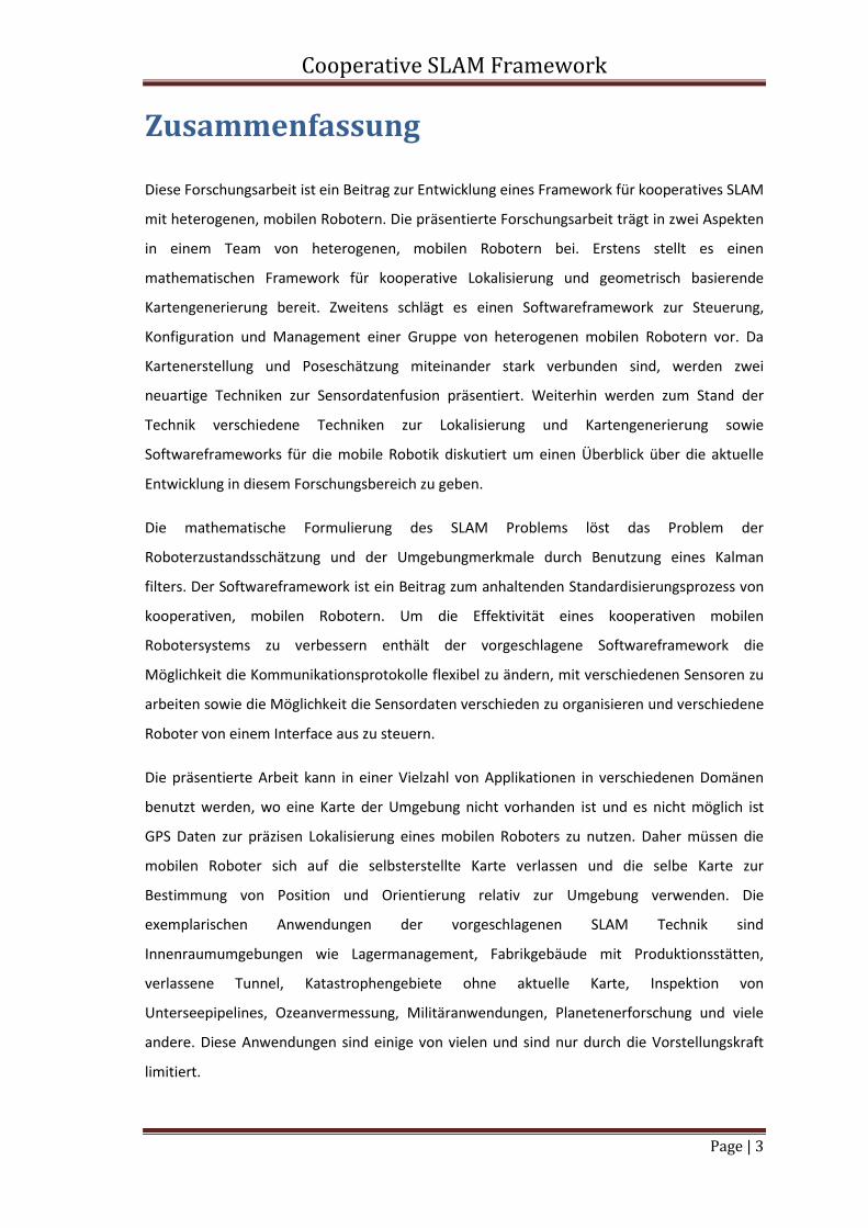
Zusammenfassung
Diese Forschungsarbeit ist ein Beitrag zur Entwicklung eines Framework für kooperatives SLAM
mit heterogenen, mobilen Robotern. Die präsentierte Forschungsarbeit trägt in zwei Aspekten
in einem Team von heterogenen, mobilen Robotern bei. Erstens stellt es einen
mathematischen Framework für kooperative Lokalisierung und geometrisch basierende
Kartengenerierung bereit. Zweitens schlägt es einen Softwareframework zur Steuerung,
Konfiguration und Management einer Gruppe von heterogenen mobilen Robotern vor. Da
Kartenerstellung und Poseschätzung miteinander stark verbunden sind, werden zwei
neuartige Techniken zur Sensordatenfusion präsentiert. Weiterhin werden zum Stand der
Technik verschiedene Techniken zur Lokalisierung und Kartengenerierung sowie
Softwareframeworks für die mobile Robotik diskutiert um einen Überblick über die aktuelle
Entwicklung in diesem Forschungsbereich zu geben.
Die mathematische Formulierung des SLAM Problems löst das Problem der
Roboterzustandsschätzung und der Umgebungmerkmale durch Benutzung eines Kalman
filters. Der Softwareframework ist ein Beitrag zum anhaltenden Standardisierungsprozess von
kooperativen, mobilen Robotern. Um die Effektivität eines kooperativen mobilen
Robotersystems zu verbessern enthält der vorgeschlagene Softwareframework die
Möglichkeit die Kommunikationsprotokolle flexibel zu ändern, mit verschiedenen Sensoren zu
arbeiten sowie die Möglichkeit die Sensordaten verschieden zu organisieren und verschiedene
Roboter von einem Interface aus zu steuern.
Die präsentierte Arbeit kann in einer Vielzahl von Applikationen in verschiedenen Domänen
benutzt werden, wo eine Karte der Umgebung nicht vorhanden ist und es nicht möglich ist
GPS Daten zur präzisen Lokalisierung eines mobilen Roboters zu nutzen. Daher müssen die
mobilen Roboter sich auf die selbsterstellte Karte verlassen und die selbe Karte zur
Bestimmung von Position und Orientierung relativ zur Umgebung verwenden. Die
exemplarischen Anwendungen der vorgeschlagenen SLAM Technik sind
Innenraumumgebungen wie Lagermanagement, Fabrikgebäude mit Produktionsstätten,
verlassene Tunnel, Katastrophengebiete ohne aktuelle Karte, Inspektion von
Unterseepipelines, Ozeanvermessung, Militäranwendungen, Planetenerforschung und viele
andere. Diese Anwendungen sind einige von vielen und sind nur durch die Vorstellungskraft
limitiert.
Cooperative SLAM Framework
Page | 4
Acknowledgement
This research work is a result of my endeavor as a PhD student at department of
Elektrotechnik und Informatik, University of Siegen, Germany. During my effort I have been
supported by many people to whom I wish to express my gratitude.
First of all, I would like to acknowledge the support of my wife Ayesha during my PhD time
period. I can’t describe in words all the ways in which she encouraged me. I would also like to
acknowledge the contribution of my parents, brothers and sisters to support me at every stage
of my life and for their moral supports and fond memories.
Especially, I am indebted to Prof. Dr. –Ing. Hubert Roth for providing me a possibility at the
institute of control techniques at university of Siegen. I would like to thank him for providing
me assistance and freedom to conduct my research work throughout the past three and half
years of my doctoral research work. The institute of control engineering department provided
me a conducive environment to learn and the resources to perform experiment that resulted
in this research work. I would also like to specially thank my colleague Christof Hille for fruitful
discussions regarding many issues. Furthermore, I thank Prof. Dr. rer. nat. Klaus Schilling for
being my second supervisor. I would also like to thank Prof. Dr.-Ing. habil. R. Obermaisser,
Prof. Dr. Roland Wismüller for being my co-examiner in the PhD committee.
At the end I would like to thank HEC Pakistan and DAAD to provide me a scholarship to finish
my PhD studies at university of Siegen.
To my lovely family
Cooperative SLAM Framework
Page | 5
Table of Contents
Abstract ......................................................................................................................................... 2
Zusammenfassung ........................................................................................................................ 3
Acknowledgement ........................................................................................................................ 4
Table of Contents .......................................................................................................................... 5
List of Figures ................................................................................................................................ 9
List of Tables ................................................................................................................................ 11
Notations ..................................................................................................................................... 12
Chapter 1. Introduction ........................................................................................................... 14
1.1. Motivation ................................................................................................................. 14
1.2. Problem Statement .................................................................................................... 15
1.3. Research Work Scope ................................................................................................ 15
1.4. Related Works ........................................................................................................... 16
1.5. Methodology ............................................................................................................. 21
1.6. Applications ............................................................................................................... 22
1.7. Thesis Overview ......................................................................................................... 23
Chapter 2. Theory and Background ........................................................................................ 24
2.1. Probabilistic Motion Model ....................................................................................... 25
2.1.1. Robot Motion Model Using Wheel Odometry ...................................................... 26
2.2. Probabilistic Observation Model ............................................................................... 28
2.2.1. Observation Model Using Range Sensors ............................................................. 30
2.3. Estimation .................................................................................................................. 30
2.3.1. Extended Kalman Filter ......................................................................................... 31
2.3.2. Particle Filter ......................................................................................................... 33
2.4. Localization ................................................................................................................ 35
2.4.1. Pose Estimation ..................................................................................................... 35
2.5. Mapping ..................................................................................................................... 40
Cooperative SLAM Framework
Page | 6
2.5.1. Grid Based Mapping .............................................................................................. 40
2.5.2. Feature Based Mapping ........................................................................................ 42
2.6. Navigation .................................................................................................................. 48
2.6.1. Implementation ..................................................................................................... 51
2.7. Summary .................................................................................................................... 52
Chapter 3. Simultaneous Localization and Mapping .............................................................. 53
3.1. SLAM .......................................................................................................................... 53
3.2. Prediction .................................................................................................................. 54
3.3. Correction .................................................................................................................. 56
3.3.1. Clustering or Segmentation .................................................................................. 56
3.3.2. Feature Extraction ................................................................................................. 59
3.3.3. Feature prediction from map ................................................................................ 66
3.3.4. Map Update .......................................................................................................... 68
3.3.5. New Features ........................................................................................................ 68
3.4. Summary .................................................................................................................... 70
Chapter 4. Cooperative SLAM (CSLAM) .................................................................................. 71
4.1. SLAM for Heterogeneous features ............................................................................ 71
4.1.1. Prediction .............................................................................................................. 72
4.1.2. Update ................................................................................................................... 72
4.1.3. New Plane Features .............................................................................................. 74
4.2. SLAM for Multiple robot with known initial poses .................................................... 75
4.3. Summary .................................................................................................................... 76
Chapter 5. Framework and Hardware Development.............................................................. 77
5.1. Overview of the system ............................................................................................. 78
5.1.1. Control Center ....................................................................................................... 80
5.1.2. Coordinator ........................................................................................................... 82
5.1.3. Agents.................................................................................................................... 91
5.2. Firmware and Hardware ............................................................................................ 92
Cooperative SLAM Framework
Page | 7
5.2.1. Firmware ............................................................................................................... 92
5.2.2. Hardware ............................................................................................................... 94
5.3. Simulation Environment ............................................................................................ 95
5.4. Summary .................................................................................................................... 98
Chapter 6. Experiment and Results ......................................................................................... 99
6.1. Setup .......................................................................................................................... 99
6.2. Map Management and Feature Fusion ................................................................... 101
6.3. Cooperative SLAM ................................................................................................... 103
6.4. Resultant Map ......................................................................................................... 104
6.5. Summary .................................................................................................................. 105
Chapter 7. Discussion ............................................................................................................ 106
7.1. Outlook .................................................................................................................... 107
7.2. Contributions ........................................................................................................... 108
7.3. Future Works ........................................................................................................... 109
Appendix A ................................................................................................................................ 110
Encoder Velocity Error Model ............................................................................................... 110
Accelerometer Velocity Error Model .................................................................................... 110
Gyroscope Error Model ......................................................................................................... 111
Compass Angle Error Model ................................................................................................. 111
Appendix B ................................................................................................................................ 112
Least Square Estimation ........................................................................................................ 112
Appendix C ................................................................................................................................ 115
Appendix D ................................................................................................................................ 118
Create an C# based TCP/IP Client to communicate with a simulated robot in USARSim ..... 118
Setting up a Simulation Environment ................................................................................... 118
Running Simulation Environment ......................................................................................... 118
Communication with game engine ....................................................................................... 118
Client Application .................................................................................................................. 119
Cooperative SLAM Framework
Page | 8
ProcessRxData ....................................................................................................................... 120
DisplayData ........................................................................................................................... 121
Important Commands and Messages Format ...................................................................... 121
Messages ............................................................................................................................... 121
STA .................................................................................................................................... 121
SEN .................................................................................................................................... 122
Commands ............................................................................................................................ 124
INIT .................................................................................................................................... 124
DRIVE ................................................................................................................................. 125
Appendix E ................................................................................................................................ 126
Simulation of Map Building in ROS with Mobile Robots Equipped with Odometry and Laser
Range Scanner....................................................................................................................... 126
Bibliography .............................................................................................................................. 128
Cooperative SLAM Framework
Page | 9
List of Figures
Figure 1.1 Simulation of Pioneer Robot in PSG Environment ..................................................... 18
Figure 1.2 Simulation of virtual robot in Stage-ROS ................................................................... 19
Figure 1.3 Sensor measurement visualization in RVIZ-ROS ........................................................ 19
Figure 1.4 Simulation of aerial and ground robot in a virtual environment based on Unreal
Tournament game engine ........................................................................................................... 20
Figure 1.5: Microsoft Robotics Studio simulation of multiple robots ......................................... 20
Figure 1.6 Marilou based mobile robot simulation .................................................................... 21
Figure 1.7 Webbot based simulation of Poineer mobile robot .................................................. 21
Figure 2.1 Mobile robot odometry process ................................................................................ 27
Figure 2.2 Direct Pre-Filtering ..................................................................................................... 36
Figure 2.3 Indirect Feed Backward Filtering ............................................................................... 36
Figure 2.4 Direct Filtering ............................................................................................................ 36
Figure 2.5 Indirect Feed Forward Filtering .................................................................................. 36
Figure 2.6 Block diagram for multi-sensor data fusion for mobile robot's pose estimation ...... 37
Figure 2.7 Experiment Environment with ferromagnetic interferences and reference wall for
measurements ............................................................................................................................ 38
Figure 2.8 Trajectory estimation by wheels encoders , PMD Camera and fusion algorithm ..... 38
Figure 2.9 Stereo Camera and Gyroscope Setup on TOM3D ...................................................... 39
Figure 2.10 Stereo-Gyro Data Fusion Flowchart ......................................................................... 39
Figure 2.11 Experiment trajectory for Stereo-Gyro data fusion experiment ............................. 39
Figure 2.12 Stereo-Gyro data fusion experiment result ............................................................. 39
Figure 2.13 Manual occupancy grid map creation ...................................................................... 40
Figure 2.14 Automatic occupancy grid map creation ................................................................. 40
Figure 2.15 Original map image of the environment .................................................................. 43
Figure 2.16 Extracted line features from the map image ........................................................... 43
Figure 2.17 Robot trajectory in the mapped environment ......................................................... 46
Figure 2.18 Geometric map created using Hough transformation ............................................. 47
Figure 2.19 Geometric map created using RANSAC algorithm ................................................... 47
Figure 2.20 Visual comparison of three path finding algorithms in scenerio-1 .......................... 49
Figure 2.21 Visual comparison of three path finding algorithms in scenerio-2 .......................... 50
Figure 3.1 Simulation of range-bearing based EKF SLAM ........................................................... 53
Figure 3.2 Simulated environment for evaluating different segmentation algorithms .............. 57
Cooperative SLAM Framework
Page | 10
Figure 3.3 Plane definition in Hessian normal form ................................................................... 64
Figure 5.1 Heterogeneous mobile robots cooperation for map building in a partially structured
environment ............................................................................................................................... 78
Figure 5.2 Cooperative heterogeneous multi-robot network architecture................................ 79
Figure 5.3 Ground mobile coordinator graphical user interface ................................................ 83
Figure 5.4 Ground mobile robot's communication module setting interface ............................ 84
Figure 5.5 Ground mobile robot's electronic compass settings ................................................ 84
Figure 5.6 Ground mobile robot's motor controller settings .................................................... 85
Figure 5.7 Ground mobile robot's ultrasonic sensor settings .................................................... 85
Figure 5.8 PID controller settings for the left and right motors of the selected differential drive
robot ........................................................................................................................................... 86
Figure 5.9 Settings related to ground mobile robot coordinator ............................................... 86
Figure 5.10 Communication packet debugging interface ........................................................... 87
Figure 5.11 Add/Edit Ground mobile robot configuration ......................................................... 88
Figure 5.12 Structure of the database tables ............................................................................. 89
Figure 5.13 Online cooperative map generator utility ............................................................... 90
Figure 5.14 Ground mobile coordinator’s local grid map ........................................................... 90
Figure 5.15 Tom3D ground mobile robot ................................................................................... 91
Figure 5.16 Tracked Merlin ground mobile robot....................................................................... 91
Figure 5.17 Hardware of general purpose ground robots control board ................................... 94
Figure 5.18 Agents Communication Modem based on IEEE 802.15.4 ........................................ 95
Figure 5.19 Aerial and Ground Robot Cooperative Localization In USARSim ............................. 96
Figure 5.20 Plan view of simulation environment in USARSim .................................................. 97
Figure 6.1 Cooperative SLAM experiment's simulation setup .................................................... 99
Figure 6.2 Waypoint navigation for differential drive mobile robot ........................................ 101
Figure 6.3 Two non-overlapping line segments with same parameters .................................. 102
Figure 6.4 Projection of line segment's end points for overlapping check ............................... 102
Figure 6.5 Cooperative EKF-SLAM generated line feature map ............................................... 104
Figure 0.1 An example client application receiving simulation data ........................................ 119
Cooperative SLAM Framework
Page | 11
List of Tables
Table 2.1 Occupancy Grid Map XML Output file's format .......................................................... 41
Table 3.1 Randomized Hough transform algorithm.................................................................... 65
Table 5.1 General communication packet structure ................................................................. 80
Table 5.2 General module related settings ................................................................................. 83
Table 5.3 General module related commands ............................................................................ 86
Table 5.4 Pseudo-code for modular robot firmware .................................................................. 94
Table 6.1 Cooperative EKF-SLAM Pseudocode ......................................................................... 103

Cooperative SLAM Framework
Page | 12
Notations
Following acronyms and notations are used throughout this text. Vectors are represented by
lower subscripted letters ( ) where the matrices are represented by capital letters (A, B, C,
K). The notation of is used for the mobile robot pose instead of the x coordinate of the
position. Sometime the term single robot is used instead of multiple robots just for bringing
clarity and simplicity to the discussion.
CDF Cumulative Distribution Function
CUDA Compute Unified Device Architecture
EKF Extended Kalman Filter
FBM Feature Based Map
FOV Field of View
GPS Global Positioning System
GPU Graphical Processing Unit
GT Ground Truth
HSM Hessian Scan Matching algorithm
ICP Iterative Closest Point matching algorithm
IMU Inertial Measurement Unit
KF Kalman Filter
LASER Light Amplification by Stimulated Emission of Radiation
LIDAR/LADAR LIght Detection and Ranging
MSRS MicroSoft Robotics Studio
OGM Occupancy Grid Mapping
PDF Probability Distribution Function
Cooperative SLAM Framework
Page | 13
PF Particle Filter
PSM Polar coordinate Scan Matching algorithm
RBPF Rao-Blackwellised Particle Filter
RFID Radio Frequency IDentification
RGB-D Red Green Blue – Depth device such as Microsoft Kinect
ROS Robot Operating System
SIFT Scale Invariant Feature Transform
SONAR SOund Navigation and Ranging
SURF Speeded Up Robust Features
TCP Transmission Control Protocol
UDP User Datagram Protocol
Cooperative SLAM Framework
Page | 14
Chapter 1.
Introduction
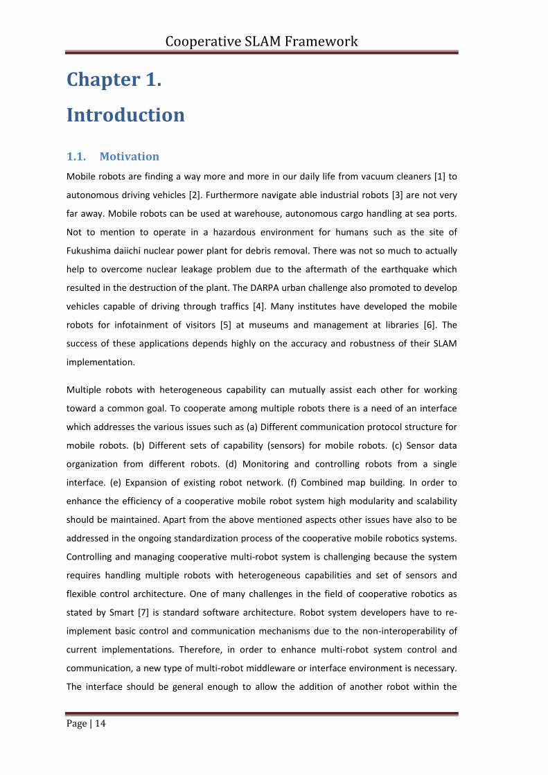
1.1. Motivation
Mobile robots are finding a way more and more in our daily life from vacuum cleaners [1] to
autonomous driving vehicles [2]. Furthermore navigate able industrial robots [3] are not very
far away. Mobile robots can be used at warehouse, autonomous cargo handling at sea ports.
Not to mention to operate in a hazardous environment for humans such as the site of
Fukushima daiichi nuclear power plant for debris removal. There was not so much to actually
help to overcome nuclear leakage problem due to the aftermath of the earthquake which
resulted in the destruction of the plant. The DARPA urban challenge also promoted to develop
vehicles capable of driving through traffics [4]. Many institutes have developed the mobile
robots for infotainment of visitors [5] at museums and management at libraries [6]. The
success of these applications depends highly on the accuracy and robustness of their SLAM
implementation.
Multiple robots with heterogeneous capability can mutually assist each other for working
toward a common goal. To cooperate among multiple robots there is a need of an interface
which addresses the various issues such as (a) Different communication protocol structure for
mobile robots. (b) Different sets of capability (sensors) for mobile robots. (c) Sensor data
organization from different robots. (d) Monitoring and controlling robots from a single
interface. (e) Expansion of existing robot network. (f) Combined map building. In order to
enhance the efficiency of a cooperative mobile robot system high modularity and scalability
should be maintained. Apart from the above mentioned aspects other issues have also to be
addressed in the ongoing standardization process of the cooperative mobile robotics systems.
Controlling and managing cooperative multi-robot system is challenging because the system
requires handling multiple robots with heterogeneous capabilities and set of sensors and
flexible control architecture. One of many challenges in the field of cooperative robotics as
stated by Smart [7] is standard software architecture. Robot system developers have to re-
implement basic control and communication mechanisms due to the non-interoperability of
current implementations. Therefore, in order to enhance multi-robot system control and
communication, a new type of multi-robot middleware or interface environment is necessary.
The interface should be general enough to allow the addition of another robot within the
Cooperative SLAM Framework
Page | 15
network with a different set of sensors and communication protocols. Furthermore, sensor
data from different robots should be organized and managed in a structured way. The overall
system should be flexible enough to be adopted for the need of robot control.
It is exciting to know how the multiple robots can help each other to solve the SLAM problem,
therefore the research work has two ambitions, first is to develop a framework where multiple
robots can cooperative with each other. The second is to develop a mathematical SLAM
framework for building a centralized geometric map cooperatively. Although many algorithms
exist today to solve SLAM problems for single mobile robot in static indoor environment, there
is still a challenge to perform cooperative SLAM especially the map merging part. The large,
dynamic, sparse and outdoor environment makes the problem further interesting. This
research work proposes a cooperative SLAM framework which addresses the issues of
cooperative SLAM and building a software framework for cooperation among heterogeneous
mobile robots.
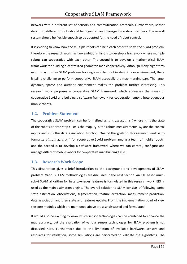
1.2. Problem Statement
The cooperative SLAM problem can be formalized as ( | ) where is the state
of the robots at time step , is the map, is the robots measurements, are the control
inputs and is the data association function. One of the goals in this research work is to
formalize ( | ) for cooperative SLAM problem among a team of mobile robots,
and the second is to develop a software framework where we can control, configure and
manage different mobile robots for cooperative map building tasks.
1.3. Research Work Scope
This dissertation gives a brief introduction to the background and developments of SLAM
problem. Various SLAM methodologies are discussed in the next section. An EKF based multi-
robot SLAM algorithm for heterogeneous features is formulated in this research work. EKF is
used as the main estimation engine. The overall solution to SLAM consists of following parts;
state estimation, observations, segmentation, feature extraction, measurement prediction,
data association and then state and features update. From the implementation point of view
the core modules which are mentioned above are also discussed and formulated.
It would also be exciting to know which sensor technologies can be combined to enhance the
map accuracy, but the evaluation of various sensor technologies for SLAM problem is not
discussed here. Furthermore due to the limitation of available hardware, sensors and
resources for validation, some simulations are performed to validate the algorithms. The
Cooperative SLAM Framework
Page | 16
research work scope is also limited for indoor environment. The cooperative SLAM algorithm
discussed in Chapter 4 assumes that the initial relative robot poses are known.
1.4. Related Works
SLAM in literature is often referred as chicken or the egg causality dilemma. Much research
has been done on this topic over the past decades as Hugh Durrant-Whyte [8] states that a
solution of SLAM problem is the Holy Grail for the mobile robotics community. SLAM is a hard
problem because of big and dynamic robot environment, robot’s noisy sensors measurements
and robot’s motion and control errors. A solution of the SLAM problem requires a big state
vector consisting of robot pose and position of all landmarks, which represent the world
around the mobile robot. This state vector is updated each time new measurement from the
robot sensors are available, therefore, it requires a lot of computational power. SLAM can be
performed either using environment features or using scan matching technique in which raw
sensor measurements are used. The feature based SLAM is the earlier version of the SLAM
which was realized using an EKF. In a scan matching technique one need’s to estimate a
transformation which consists of a rotation and translation to find relative pose of the robot
between two consecutive raw sensor measurements. Many scan matching techniques exists in
the literature such as ICP [9], HSM [10] and PSM [11]. For a comparison among different scan
matching techniques please refer [12].
The inception of the probabilistic SLAM problem occurred during mid-80’s [8]. The research
work by Smith et al [13] and Durrant-Whyte [14] described probabilistic estimation technique
for correlation among map features and robot pose. The key insight of the high correlation
among map features (landmarks) and robot pose described that, these correlations grows with
successive continuous observations. Crowley [15] and Leonard [16] performed SLAM using
sonar sensors. They used the line segments extracted from ultrasonic sensor data as features.
Vandorpe [17] and Gonzalez [18] used laser data to perform SLAM. During that time Faugeras
[19] and Ayache performed earliest work in visual navigation and mapping. Lenord [20]
worked on to reduce the computational requirements by dividing the state vector into local
sub parts. This idea was skipped when later on it was found that for the convergence of the
SLAM problem, the huge state-vector is essential and more the correlation among features
grows the better solution becomes. So far, the robots pose and landmarks were represented
by univariate Gaussian noise model. Murphy [21] introduced a particle filter which is a
discretized representation of a complex multi-model probability density function. Using
particle filters the robot pose is represented by a set of discrete states, particles. He
Cooperative SLAM Framework
Page | 17
furthermore proposed the discretization of the space around the robot in blocks which he
termed as occupancy grid mapping. Later on, Montemerlo [22] extended the work to feature
based maps, which is known as FastSLAM in which he used Extended Kalman filter to estimate
the map where particle filter was used to represent robot pose. GMapping [23] is a grid based
SLAM algorithm in 2D. The first working solution of the SLAM problem was based on extended
Kalman filter (EKF-SLAM) and then later came the Rao-Blackwellised particle filter (FastSLAM).
The main advantage of a particle filter is to represent a multi model belief about robot states.
Many authors like [24] [23] [25] uses grid based maps with PF to address the SLAM problem in
large dynamic outdoor environment. Grisetti [23] developed GMapping which is at the
moment a very robust tool to build the grid map using a laser scanner and odometry. Haehnel
[25] proposed GridSLAM algorithm and Eliazer [24] proposed DP-SLAM. GMapping and
GridSLAM reduce the number of particles where DP-SLAM uses a tree based structure. Many
of state of the art SLAM algorithm are available on OpenSLAM [26] website as open source
packages, furthermore many of the algorithms are also available as ROS [27] packages.
There are many challenges in cooperative SLAM such as a standard framework for data
acquisition, robot and their sensor data management, global map representation and the
mathematical framework for fusing multi-robot and multi-sensor data. In general cooperative
slam can be performed in a centralized [28] [29] or decentralized [30] [31] [32] [33] manner.
Jayasekara [34] proposed a method for cooperation based on external tracking of robots
which is limited to visual range of the camera and laser scanner. Williams [35] proposed a
decentralized cooperative SLAM methodology to manage computational complexity and
improved data association. Andrew [31] proposed the method of decentralized cooperative
SLAM based on FASTSLAM. The map merging part is performed only when one robot detects
other and measures its pose relative to its own. This situation happens less frequent in
practical scenarios. Lee [36] proposed the distributed cooperative SLAM using the ceiling
vision. Using ceiling vision based data association technique the proposed algorithm detects
the overlapping regions, an estimate of the transformation for map alignment. This technique
is limited to indoor planer environment. Zhou [37] proposed an algorithm for multi-robot map
alignment to build a joint map. Relative pose measurement between robots is used to find the
transformation between maps. When there is an overlap between maps i.e. landmarks appear
twice in two maps this information helps to increase the map alignment accuracy. Ming [38]
proposed a cooperative SLAM technique using vertical lines and colored name plates as
landmarks in an indoor office environment.
Cooperative SLAM Framework
Page | 18
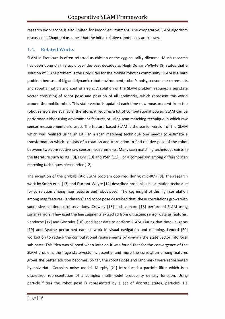
Figure 1.1 Simulation of Pioneer Robot in PSG Environment
Regarding a standard framework for mobile robotics, many set of libraries and tools exist for
handling mobile robots. Many of them focus on the single mobile robot while other targets a
group of robots but usually such frameworks are application and platform dependent. The
player project [39] is a popular open source robot software framework which handles the
communication between robot hardware/simulation and the control software clients. PSG
(Player Stage Gazebo) consists of a 2D simulator “Stage”, a 3D simulator “Gazebo” [40] as
shown in Figure 1.1 and robot control interface software “Player”. Its client server architecture
is based on TCP sockets. The mobile robot’s hardware is accessed through drivers and many of
the drivers are already implemented in Player, furthermore, PSG can be used for simulating
robots. For implementation of player drivers for a custom robot please refer to [41]. Few
weakness of PSG systems are as follows. In order to function properly, Gazebo has many non-
documented dependencies that include specific versions of the third party libraries. Another
important deficiency of Gazebo is that there is no online mesh generation and rendering
capability which is important for creating online maps from mobile robots range sensors data.
Unfortunately overall PSG system is difficult to install and run due to its complexity [42] and
non-documented dependencies, furthermore, it does not provide online map making facility
and no structured built-in scheme for storage of robots data.
During STAIR project [43] at Stanford it was also required and realized such a software
framework for hardware software integration of various mobile robot modules which later
evolved into ROS [44]. ROS [27] is an open source project which provides a framework for
communicating data within various running processes and uses existing source code and
libraries for managing robot related tasks. It uses IPC (Inter Process Communication)
methodology for peer to peer communication among various nodes (executable); therefore,
modules do not require to be linked together in one executable. Messages among nodes are
communicated through master node; therefore publisher (sender) and listener (receiver) both
Cooperative SLAM Framework
Page | 19
are unaware of their existence. Nodes for ROS can be written either using C++ or Python. The
ROS specifications are at messaging layer for cross-language development. ROS has various
tools for managing, building and running various ROS components. It uses other open source
projects code such as PSG for simulation, OpenCV for vision sensors, OpenNI for RGB-D
camers, Eigen for matrix algebra libraries and many more. It also provides a data logging and
playback mechanism which is missing in PSG system which is a very important aspect for a
multi robot system during development. For a conceptual working about ROS system please
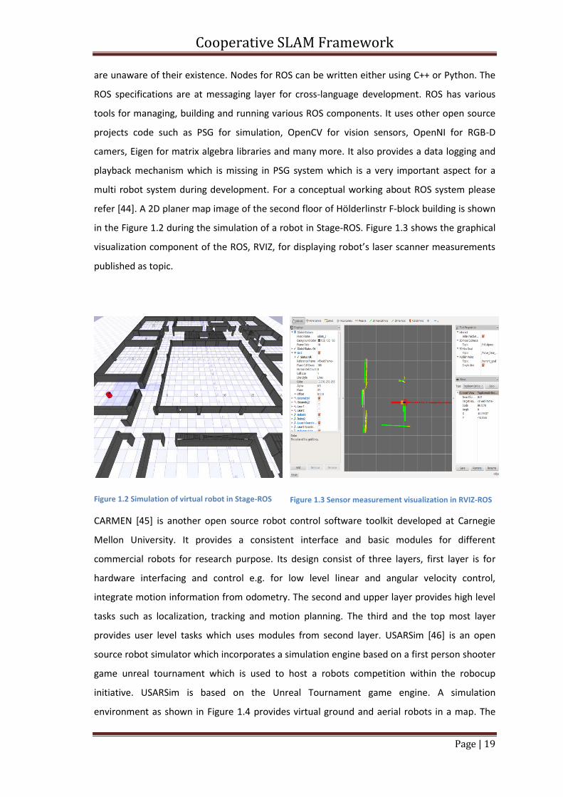
refer [44]. A 2D planer map image of the second floor of Hölderlinstr F-block building is shown
in the Figure 1.2 during the simulation of a robot in Stage-ROS. Figure 1.3 shows the graphical
visualization component of the ROS, RVIZ, for displaying robot’s laser scanner measurements
published as topic.
Figure 1.2 Simulation of virtual robot in Stage-ROS
Figure 1.3 Sensor measurement visualization in RVIZ-ROS
CARMEN [45] is another open source robot control software toolkit developed at Carnegie
Mellon University. It provides a consistent interface and basic modules for different
commercial robots for research purpose. Its design consist of three layers, first layer is for
hardware interfacing and control e.g. for low level linear and angular velocity control,
integrate motion information from odometry. The second and upper layer provides high level
tasks such as localization, tracking and motion planning. The third and the top most layer
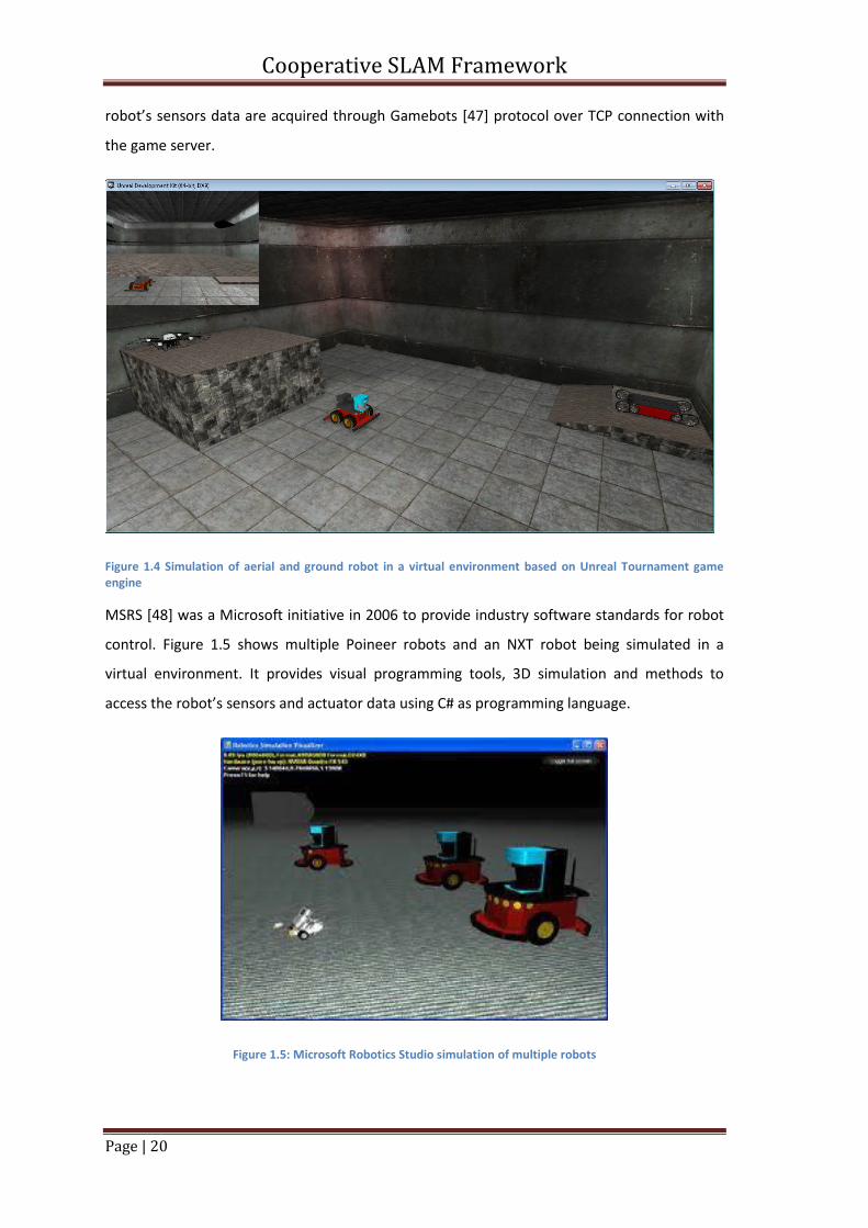
provides user level tasks which uses modules from second layer. USARSim [46] is an open
source robot simulator which incorporates a simulation engine based on a first person shooter
game unreal tournament which is used to host a robots competition within the robocup
initiative. USARSim is based on the Unreal Tournament game engine. A simulation
environment as shown in Figure 1.4 provides virtual ground and aerial robots in a map. The
Cooperative SLAM Framework
Page | 20
robot’s sensors data are acquired through Gamebots [47] protocol over TCP connection with
the game server.
Figure 1.4 Simulation of aerial and ground robot in a virtual environment based on Unreal Tournament game engine
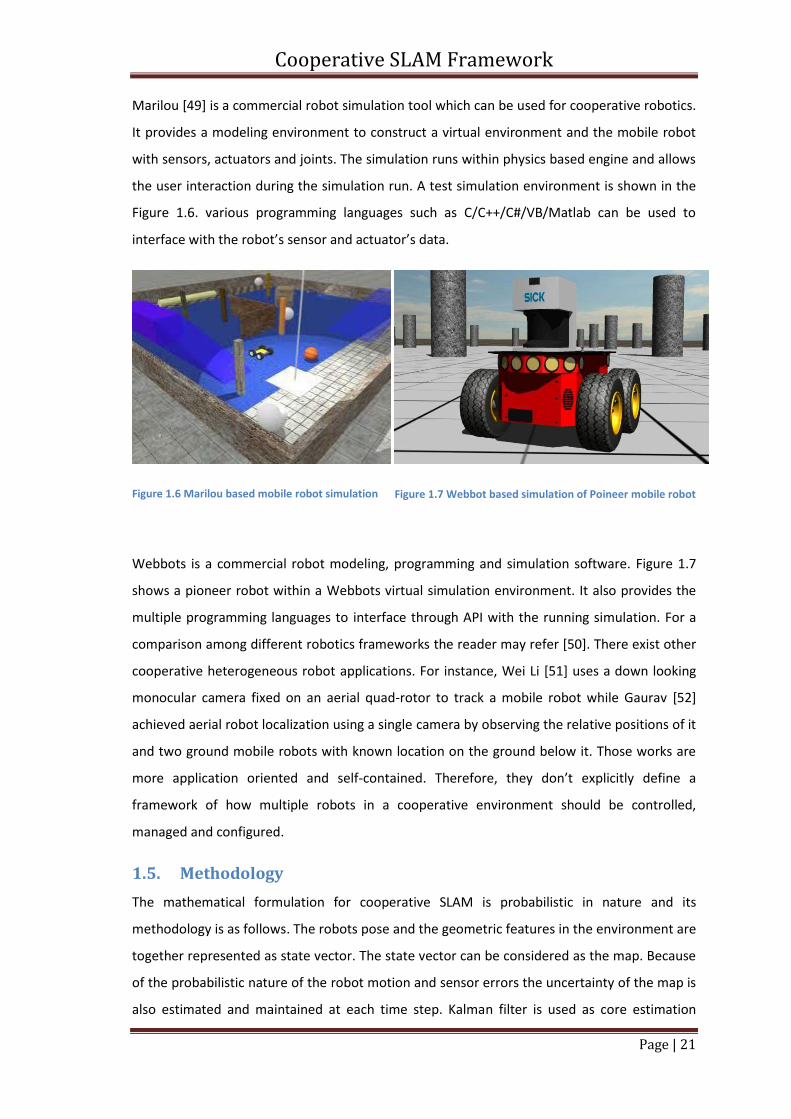
MSRS [48] was a Microsoft initiative in 2006 to provide industry software standards for robot
control. Figure 1.5 shows multiple Poineer robots and an NXT robot being simulated in a
virtual environment. It provides visual programming tools, 3D simulation and methods to
access the robot’s sensors and actuator data using C# as programming language.
Figure 1.5: Microsoft Robotics Studio simulation of multiple robots
Cooperative SLAM Framework
Page | 21
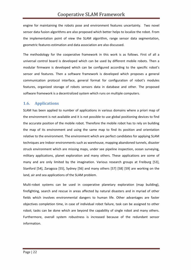
Marilou [49] is a commercial robot simulation tool which can be used for cooperative robotics.
It provides a modeling environment to construct a virtual environment and the mobile robot
with sensors, actuators and joints. The simulation runs within physics based engine and allows
the user interaction during the simulation run. A test simulation environment is shown in the
Figure 1.6. various programming languages such as C/C++/C#/VB/Matlab can be used to
interface with the robot’s sensor and actuator’s data.
Figure 1.6 Marilou based mobile robot simulation
Figure 1.7 Webbot based simulation of Poineer mobile robot
Webbots is a commercial robot modeling, programming and simulation software. Figure 1.7
shows a pioneer robot within a Webbots virtual simulation environment. It also provides the
multiple programming languages to interface through API with the running simulation. For a
comparison among different robotics frameworks the reader may refer [50]. There exist other
cooperative heterogeneous robot applications. For instance, Wei Li [51] uses a down looking
monocular camera fixed on an aerial quad-rotor to track a mobile robot while Gaurav [52]
achieved aerial robot localization using a single camera by observing the relative positions of it
and two ground mobile robots with known location on the ground below it. Those works are
more application oriented and self-contained. Therefore, they don’t explicitly define a
framework of how multiple robots in a cooperative environment should be controlled,
managed and configured.
1.5. Methodology
The mathematical formulation for cooperative SLAM is probabilistic in nature and its
methodology is as follows. The robots pose and the geometric features in the environment are
together represented as state vector. The state vector can be considered as the map. Because
of the probabilistic nature of the robot motion and sensor errors the uncertainty of the map is
also estimated and maintained at each time step. Kalman filter is used as core estimation
Cooperative SLAM Framework
Page | 22
engine for maintaining the robots pose and environment features uncertainty. Two novel
sensor data fusion algorithms are also proposed which better helps to localize the robot. From
the implementation point of view the SLAM algorithm, range sensor data segmentation,
geometric features estimation and data association are also discussed.
The methodology for the cooperative framework in this work is as follows. First of all a
universal control board is developed which can be used by different mobile robots. Then a
modular firmware is developed which can be configured according to the specific robot’s
sensor and features. Then a software framework is developed which proposes a general
communication protocol interface, general format for configuration of robot’s modules
features, organized storage of robots sensors data in database and other. The proposed
software framework is a decentralized system which runs on multiple computers.
1.6. Applications
SLAM has been applied to number of applications in various domains where a priori map of
the environment is not available and it is not possible to use global positioning devices to find
the accurate position of the mobile robot. Therefore the mobile robot has to rely on building
the map of its environment and using the same map to find its position and orientation
relative to the environment. The environment which are perfect candidates for applying SLAM
techniques are Indoor environments such as warehouse, mapping abandoned tunnels, disaster
struck environment which are missing maps, under see pipeline inspection, ocean surveying,
military applications, planet exploration and many others. These applications are some of
many and are only limited by the imagination. Various research groups at Freiburg [53],
Stanford [54], Zaragoza [55], Sydney [56] and many others [57] [58] [59] are working on the
land, air and sea applications of the SLAM problem.
Multi-robot systems can be used in cooperative planetary exploration (map building),
firefighting, search and rescue in areas affected by natural disasters and in myriad of other
fields which involves environmental dangers to human life. Other advantages are faster
objectives completion time, in case of individual robot failure, task can be assigned to other
robot; tasks can be done which are beyond the capability of single robot and many others.
Furthermore, overall system robustness is increased because of the redundant sensor
information.
Cooperative SLAM Framework
Page | 23
1.7. Thesis Overview
This thesis is structured as follows; Chapter 1 describes the background and motivation of the
research work. It describes also the problem statement, research scope and the related work
in this field in chronological order.
Chapter 2 describes the required tools and techniques to solve the SLAM problem. It also
discusses the individual components of the SLAM solution algorithm such as localization,
mapping and navigation. Since the mapping is closely dependent on robot’s pose therefore,
two novel pose estimation techniques are also discussed.
Chapter 3 discusses the extended Kalman filter based SLAM approach and its core components
in detail. These components are clustering or segmentation, geometric feature extraction,
data association or map update and the augmentation of new features into the map.
Chapter 4 discusses the EKF based SLAM process for multiple robots and heterogeneous
features.
In Chapter 5 a cooperative SLAM software framework for multiple robots is discussed. It
describes the architecture and components of the system, firmware and hardware
components for mobile robots. It also describes a simulation environment which can be used
for the rapid development of the mobile robots related cooperative SLAM algorithms.
Chapter 6 discusses the implementation of the proposed cooperative architecture on the
robot. It discusses the implemented framework and the applied cooperative SLAM algorithm.
Chapter 7 ends the thesis with a discussion about the research work and concludes with the
future work direction.
Cooperative SLAM Framework
Page | 24
Chapter 2.
Theory and Background
This chapter provides the theoretical bases, mathematical tools and techniques required for
this research work. These theoretical backgrounds are not complete in it-self, therefore, for an
in-depth understanding the reader is suggested to refer the corresponding references
mentioned in the text.
Here we will discuss the structure of the SLAM which is often implemented in Bayesian form.
The Bayes rule can be represented in the following form:
( | ) ( | ) ( | )
( | ) Eq. 2.1
Here, ( | ) represent the posterior probability, ( | ) represents the prior
probability, ( | ) represents the conditional probability of given
and . ( | ) is the normalization constant which is often written as in the
literature. In the above equation denotes the robot pose at time step t, represents all
the observations and represents all the control commands, linear and angular velocity.
The two important assumptions which play an important role in probabilistic robotics are
Markov process model and the Independence assumption. According to Markov process
model the current state depends only on , we silently assume the state vector is
complete, which mathematically can be described as ( | ) ( | ).
According to second assumption we will treat that each observation is independent from
the other and previous observations . After introducing the above mentioned assumption
and simplification yields the following recursive Bayes law:
( | )
( | ) ( | )
( | )
( | ) ( | )
Eq. 2.2
The term ( | ) is called the motion model where the term ( | )is called the
observation or measurement model. For further information the reader can refer [8][49].
Cooperative SLAM Framework
Page | 25
2.1. Probabilistic Motion Model
The robot motion model used in this research work assumes that the robots have holonomic
constraints such as differential drive robots and each robot wheels are separated by a
distance . If a differential drive robot is given a motion command comprises of linear and
angular velocity , - then the velocity for right and left motor velocity controller is
calculated as follows
Eq. 2.3
Eq. 2.4
Such that the positive angular velocity induces an anti-clockwise rotation and positive linear
velocity induces a forward motion. Usually a simple kinematic motion model is used for a
differential drive robot instead of a dynamic model because of the simplicity of kinematic
model and the unavailability of various parameters required for a dynamic model.
Motion model or probabilistic kinematic model for a mobile robot consists of states transition
probability distribution ( | ). It predicts the posterior distribution of mobile robot
states , which robot assumes, after applying the motion commands at prior distribution
of robot states . The states of a mobile robot consist of its pose or its configuration.
Mobile robot kinematics describes the effect of control actions on its configuration. The
configuration of a mobile robot in environment is known as its pose. The pose of a mobile
robot in 3D is described by six Degree of Freedoms (DOF), Location described by 3D Cartesian
coordinate and three Euler angles, i.e.
, - Eq. 2.5
For a mobile robot in a planar environment its pose is described by three DOF, location
described by 2D Cartesian coordinate and an orientation, i.e.
, - Eq. 2.6
The robot motion model is called probabilistic because the uncertainties in the input and/or
states are explicitly modeled into the system equations. Therefore, it is important to
understand the nature of motion noise or uncertainties which affects the robot motion. The
motion noise might be deterministic (systematic) or nondeterministic (random or non-
systematic) errors. Basically this noise is introduced because of un-modeled effects in to the
Cooperative SLAM Framework
Page | 26
robot kinematics. As we know the wheel odometry is subject to two kinds of errors, systematic
and non-systematic errors [60]. The kinematic model should be able to handle various error
sources such as different wheel diameters, inaccuracy of the wheel attachment, ground
unevenness and slip. Two systematic error sources are considered here, the difference in both
robot wheel diameters and the wheel base distance. These errors can be modeled as scale
factors and can be calculated by a calibration technique such as UMBmark [60] in an offline
manner or in an online manner [61]. In the online calibration technique these calibration scale
factors are included in the state vector and are also estimated at each time step, which is then
used to correct the odometric information. During the experimentation the ground based
mobile robot’s wheel odometry is calibrated in an offline manner by UMBmark method. The
calibration process calculates the scale factors constants, due to non-deterministic errors, that
are used to compensate the non-systematic errors in odometry information at each time step.
The non-systematic errors are random in nature and mostly happen because of slip or because
of surface morphology. These errors can be modeled as Gaussian distribution ( ) noise
with zero centered mean and standard deviation and then added to each state variable.
2.1.1. Robot Motion Model Using Wheel Odometry
Wheel odometry is obtained by integrating the wheel encoder information from ground
mobile robot. Similarly flying robot uses inertial odometry to estimate its pose which is
obtained by integrating the information obtained from inertial measurement unit but this
discussion is limited to wheel odometry. The robot’s wheel odometry information is given as
an input to the probabilistic motion model. This input can be described either by velocity or
by displacement information obtained by the right and left wheel encoders. Usually odometry
information in the form of velocity is preferred in motion planning algorithms such as collision
avoidance to predict the effect of motion in advance but here the odometry information in the
form of linear and angular displacement is used.
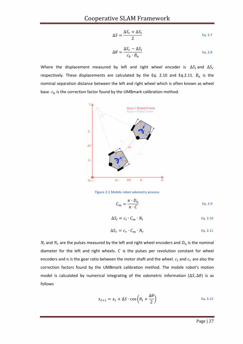
Figure 2.1 shows the kinematics of a differential drive mobile robot during a time step from
the robot pose to robot pose . Due to the linear and angular velocity command
( ) given to the robot, it will traverse a linear distance and an angle of during a
sampling interval of . The actual linear and angular displacements traversed by the mobile
robot due to the commanded velocity can be calculated by using the left and right wheels
encoder’s displacement measurements
Cooperative SLAM Framework
Page | 27
Eq. 2.7
Eq. 2.8
Where the displacement measured by left and right wheel encoder is and
respectively. These displacements are calculated by the Eq. 2.10 and Eq.2.11. is the
nominal separation distance between the left and right wheel which is often known as wheel
base. is the correction factor found by the UMBmark calibration method.
Figure 2.1 Mobile robot odometry process
Eq. 2.9
Eq. 2.10
Eq. 2.11
and are the pulses measured by the left and right wheel encoders and is the nominal
diameter for the left and right wheels. is the pulses per revolution constant for wheel
encoders and is the gear ratio between the motor shaft and the wheel. and are also the
correction factors found by the UMBmark calibration method. The mobile robot’s motion
model is calculated by numerical integrating of the odometric information ( ) is as
follows
(
) Eq. 2.12
Cooperative SLAM Framework
Page | 28
(
) Eq. 2.13
Eq. 2.14
Mathematically the complete probabilistic robot motion model using robot kinematics
including the non-deterministic effects is defined as follows
[
] [
]
[ (
)
(
)
]
[
( )
( )
( )
] Eq. 2.15
Usually one can move the robot in a predefined trajectory for calibration process. And then by
measuring the difference between robot’s absolute pose by some means and the estimated
pose using odometry process at end position during several runs, one could measure the
standard deviation of pose due to non-deterministic errors. Here is the standard
deviation of the position error, difference between absolute and estimated position, and is
the standard deviation of robot orientation error.
2.2. Probabilistic Observation Model
A probabilistic observation model ( | ) describes a process by which a sensor
measurements, landmark or feature are generated given the current robot pose and existing
map. The terms features and landmarks are synonymous in the context of SLAM and will be
used interchangeably in this text. The observation model is called probabilistic because it
accommodate the different type of deterministic and non-deterministic errors such as
measurement errors due to sensor accuracy and resolution, unexplained measurements,
failure to detect objects and unexpected objects which are not present in the existing map. As
statistically each noise source is modeled as a random variable corresponding to a particular
distribution; therefore, the probabilistic observation model is a mixture of all such
distributions. The probabilistic observation model is in fact a conditional probability which
describes the set of observations given the current robot pose and the map . Because
of independence assumption we can describe the probabilistic observation model as follows
( | ) ∏ ( | )
Eq. 2.16
The observation model depends on the type of sensor modality. SLAM algorithms rely on the
observation of the environment which is performed by various types of sensors such as range
Cooperative SLAM Framework
Page | 29
sensors, camera images and RFID signals. The accuracy and robustness of SLAM algorithms
depend on the sensor technology, further information regarding mobile robot sensors can be
found in [20]. Recent sensor technologies such as laser range scanners, RGB-D cameras and
time of flight cameras are being used now a day to map the environment of a mobile robot.
Laser beam based range sensors yield the most exact results both in indoor and outdoor
environment and therefore are commonly used. RGB-D cameras such as Microsoft Kinect [62]
and ASUS Xtion Pro [63] are limited to indoor use while the time of flight cameras have limited
field of view and range but has high frame rate therefore it is considered good candidate for
obstacle avoidance but not for SLAM. Modern laser ranger scanners are able to distinguish
among the readings which are affected while passing through the glass. We mainly used two
types of sensors, a 2D laser scanner and 3D RGB-D camera for our mobile robots. Both sensors
fall into the category of range sensors, therefore only beam based observation models will be
discussed.
The observation model also depends on the type of map; feature map or grid map. In the
feature based map the environment map can compose of certain environmental features or
location of objects in the environment. For grid based map there are three types of
observation models, beam based range models, likelihood field range model and scan
matching. Beam based range models depend mostly on the geometry and physics of the
sensor which has two drawbacks, smoothness in cluttered environment and the
computational complexity compared to the likelihood field range model. The difference
between likelihood based sensor model and scan matching is that scan matching creates a
local map of the robot to be compared with the global map which includes the free space and
open space where the likelihood based observation model only includes the end point of
range scans. All the above three sensor models are based on the raw sensor measurements.
For feature based maps the raw sensor measurements are preprocessed to extract features
along with its signatures if it is available. Mathematically we can describe the feature
extraction process as a function which is operating on the measurements, ( ) therefore,
the observation model becomes ( ( )| ). There are a number of features which can be
extracted from the environment. Usually the choice of feature is dependent on the choice of
sensor and environment. Considering range scan sensors such as laser scanner and RGB-D
cameras in partially structured indoor environment, lines, corners and planes are a good
choice of features to be extracted from raw range sensor measurements. This research work is
based on the feature based maps; therefore a simple observation model will be discussed in
the next section.
Cooperative SLAM Framework
Page | 30
2.2.1. Observation Model Using Range Sensors
The most common and basic observation model for point feature is range and bearing model.
In this model each point feature’s range and orientation relative to robot local frame are
measured by the feature extractor function along with a feature’s unique identifier or
signature. The unique identifier helps to solve the correspondence or data association
problem. The probabilistic observation model for the point feature uses the geometric laws for
range and bearing calculations, which is described by the equation 2.17 as follows
[
]
[ √( )
( )
( ) ]
[
( )
( )
( )
] Eq. 2.17
Where (
)
is the expected range, bearing and signature of measurement respectively
and ( ) is the robot pose. Each feature parameters are subjected to an uncertainty
specified as Gaussian distribution ( ). The errors in each feature’s extracted parameters
are because of the noise in the sensor measurements. Each feature is corresponds to a
feature in the map, this is called correspondence. Failure in correspondence leads to failure
of the EKF base SLAM algorithm. In case of particle filter multiple hypotheses can be tracked
simultaneously, therefore, it is more resilient to data association errors. If a measured feature
doesn’t correspond to a feature in the map then it is considered a new feature and added to
the existing map.
In case of line features first the raw measurements, one complete range scan, from the 2D
laser scanner is passed to a function for segmentation. Then the parameters of a line which is
defined in hessian normal form is estimated from each segmented cluster of range readings.
The line estimation process not only estimates the parameters of the line model but also the
uncertainty in the parameters. For detailed discussion refer section 3. Similarly the 3D plane
extraction process is described in section 3.3.2.2. The existing features are stored in a KD-tree
data structure. Therefore each observed line is searched in the KD-tree to find its
corresponding line. For the details of KD-tree data structure please refer section 3.3.3.2.
2.3. Estimation
Estimation techniques such as Extended Kalman Filter and Particle Filters are the main engine
of SLAM process. They provide us a framework to keep track of the robot and map states and
to update them as new information arrives from sensors. The estimation engines which is used
for implementing SLAM process is discussed in the following sections.
Cooperative SLAM Framework
Page | 31
2.3.1. Extended Kalman Filter
EKF localization keeps a uni-modal belief ( | ) about the localization of a mobile
robot and map features. This belief has a Gaussian distribution which can be described by its
first and second moment i.e. robot could only be at one place defined by its mean with some
uncertainty in its position defined by its variance. The uncertainty in robot position grows as
the robot moves in the environment because of noise in robot motion model. In this research
work feature based map consist of plane landmarks. The observation model for EKF which is
used depends on the type of sensor and is discussed in the next chapter. The robot motion
model used for EKF is defined in section 2.1.1.
R. E. Kalman [32] proposed a novel recursive filter technique. His proposed solution can
estimate the present, past or future states of a static/dynamic process. The Kalman filter
algorithm is a two-step algorithm which requires an appropriate model of the system under
investigation and the model of the measurements. The first step estimate the system states
according to system model where in the second step the estimated states are refined using
the observations. For in-depth knowledge about the Kalman filter and its various derivatives
the reader can refer Simon [64]. Extended Kalman filter is very popular, efficient and
computational inexpensive for a moderately small non-linear system with not so many states
and assumes that the noise present in the system is a uni-model Gaussian. A system can have
non-linarites in motion and/or observation model. Because of a non-linear robot motion
model an EKF is used. The computational expensive part of the Kalman filter is the calculation
of Kalman gains which requires an inverse of the innovation covariance matrix. This operation
has a computational cost of ( ) where is the number of states in the system. The
challenging part often in the implementation of Kalman filter is the choice of the process noise
covariance matrix parameters. Initially the non-diagonal elements, cross covariance’s, of the
covariance matrix are initialized to zero, that mean there is no correlation between robot pose
and features but as the robot start moving and start making observations the covariance
matrix becomes dense and both pose and features start becoming correlated. Correlation is
very important for convergence.
EKF follows the same cycle of prediction and correction steps. The EKF algorithm steps will be
described here in details, for detailed derivation of EKF refer [64]. The prediction or state
estimation step is described as follows
(
) Eq. 2.18
Cooperative SLAM Framework
Page | 32
Eq. 2.19
Where the Jacobian matrices and are the partial derivatives of motion model function
( ) w.r.t. states and state noise respectively as follows:
( ) Eq. 2.20
( ) Eq. 2.21
The functions is a parameter of state vector , control vector and noise vector . The
important thing to be note is that no noise is added into the state estimation. The uncertainty
due to noise is added while propagating the state covariance from the previous step. The
uncertainties in the states are modeled by the covariance matrix and it is propagated by
the motion model jacobian with respect to state noise.
The correction step of the EKF is as follows
( ) Eq. 2.22
Eq. 2.23
Eq. 2.24
Eq. 2.25
Eq. 2.26
Eq. 2.27
Eq. 2.28
is composed of the partial derivatives of measurement model w.r.t. states which is defined
as follows
( ) Eq. 2.29
Where is the expected states and is covariance of expected states. is the innovation
or the amount of new information which is brought into the system and is the innovation
covariance which is the sum of expected states covariance plus the covariance on the new
measurements. Eq. 2.26 represents the Kalman gain which is the ratio of expected states gain
Cooperative SLAM Framework
Page | 33
and the innovation gain. Eq. 2.27 and Eq. 2.28 represent the correction of the states and their
corresponding covariances. During states correction an amount of new information
proportional to Kalman gain is added to the existing states. The uncertainties of the states are
decreased proportional to the amount of Kalman gain.
2.3.2. Particle Filter
Particle filter is a very powerful tool and used for many applications such as filtering, tracking
and navigation where the system is very non-linear and state space is very large. A particle
filter is an approximation of Bayes filter which represents the robot pose by an arbitrary
multimodal probability distribution using a set of particles *
+. Each
robot pose/state/particle is associated with an importance weight/factor
which reflects
the probability or likelihood of that particle and is updated after each new observation of the
robot. The robot belief which consists of set of particles and their corresponding
importance weight is recursively updated from . First the hypothetical state estimate
, - of a sampled particle is made based on the motion model, previous particle
, - and the
control input . The likelihood of the sampled particle is proportional to the observation
probability i.e. , - . |
, -/. The observation probability is based on the difference
between the current measurement and the predicted measurement according to the stored
map of the sampled particle , -
. Secondly a resampling step is performed which is very crucial
and computationally time consuming. In this step a new particle set is created which reduces
the variance of the underlying distribution. Particles with a higher weight will appear more
often in the new list than ones with lower likelihoods which means a good hypotheses of robot
poses will remain in the non-parametric representation of the state while others disappear.
Various resampling techniques which are being employed are Multinomial Resampling,
Residual Resampling, Stratified Resampling and Systematic Resampling. For a comparison of
resampling strategies the reader is referred to [65]. For the implementation of particle filter
one can refer [66]. Resampling could also be dangerous which could lead to
deprivation/depletion problem, in which no particle exists in the vicinity of correct state. This
problem occurs when numbers of particles are small and it may happen that during
resampling good samples are replaced and the final particle distribution loses track of the
correct state. The computational effort is proportional to the number of samples. Since the
resampling step is crucial, therefore, if the robot stops or if no observations are made then it
should be avoided. GMapping [23] and DP-SLAM [67] resample only, if the particle weight
Cooperative SLAM Framework
Page | 34
variance is above a certain threshold. The particle weight variance can be calculated as
follows:
∑. , -/
⁄ Eq. 2.30
The coefficient is maximum for equal weights of the particles and resampling would not
reduce the variance of the probability distribution.
Rao-Blackwellised particle filter is a combination of EKF and PF in which the created map of
the environment consists of features (edges, corner or planes). In literature this technique is
also known as FastSLAM [66] in which the robot pose is estimated by particle filter, which
accommodate multiple hypotheses about robot position, and the features are estimated and
maintained by EKF. Since each particle represent one hypothesis of a robot pose and contains
its own set of map features describing the map. Since the map is estimated by Gaussian
therefore, each feature has a mean and variance which are represented by and
respectively. Therefore, the joint state vector for a particle is defined as follows:
, - [*
+
, -
, - , -
, - , -
, - , -] Eq. 2.31
The RB-PF can also be divided into two phases for ease of understanding, in the first phase the
particles are sampled using the motion model which is similar to simple PF approach. Then the
correspondence among observation and map features is calculated and represented by
correspondence variable . The simplest data association strategy is nearest neighbor
approach [68] with a defined distance measure. If a new feature is found its mean and
variance is calculated and added to the feature map, mean is the transformation of feature
measurement from robot local coordinate frame to global coordinate frame. Otherwise, using
the standard EKF approach its mean and covariance is propagated and the importance weight
is calculated from the innovation covariance of the feature. The resampling process is similar
to the PF. The optimized version which is known as FastSLAM 2.0 [22] basically includes the
different distribution which takes in account the current measurement into account.
The particle motion model does not implement a drift and all particle position would remain
the same while only heading angle is affected by the Gaussian noise. While in Gaussian
probabilistic motion model the position is also affected. This behavior is requested to model
the real robot kinematics. The real challenge in both cases is to find the appropriate noise
Cooperative SLAM Framework
Page | 35
control parameters. For choosing noise control parameters factors such as robot architecture,
sensor’s characteristics and environment factors should be kept in mind. In case of the particle
filter the noise has a direct influence on the variance of particle weights. Other issue in particle
filter is too often resampling which can be avoided by sampling based on the variance of the
particle filters.
2.4. Localization
The use of absolute positioning system devices/sensors obviates the localization problem.
Since the mobile robot pose cannot be determined directly because of the unavailability of
sophisticated global positioning sensors or the noise in the observations and uncertainty in
robot motion, therefore, robots pose has to be inferred from the noisy measurement
measurements. The other problem which makes the localization problem hard is the
incompleteness of a single measurement, e.g. consider a SONAR sensor can’t decide the object
shape even from a single noise free measurement which might be necessary to determine its
location with respect to that object. When there is error in the robot executed command and
actual motion performed by the robot this uncertainty will affect the future observations of
the robot because they are referenced according to robot’s local coordinate frame. Mobile
robot localization deals with determining the pose of mobile robot given the robot controls
(odometry), sensor measurement and map of the environment. Mathematically it is described
as ( | ). The environment map could be a feature based map or location based
(occupancy grid) map. A single observation is usually not enough to localize the robot within
the map, due to feature correspondence; therefore, the robot has to integrate the
observations over time to determine its pose. The severity of localization problem depends on
various factors such as the knowledge of the mobile robot’s initial position, state of the
environment, robots interaction with the environment and cooperative localization among
multiple robots. The localization algorithms here are probabilistic in nature and we will
assume the unknown correspondence, i.e. we don’t know the true identity of the detected
landmark from the robot measurement.
2.4.1. Pose Estimation
Accurate pose estimation is fundamental to mobile robots’ navigation, guidance, localization
and mapping. To compensate the characteristic deficiencies of individual sensor
measurements and to merge measurements from redundant sensors, data fusion can be
performed to get the optimal estimate of the mobile robot pose. The research work [69]
describes a method for combining data from multiple on-board sensors to determine a mobile
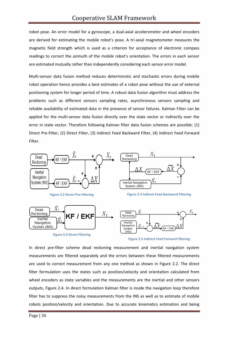
Cooperative SLAM Framework
Page | 36
robot pose. An error model for a gyroscope, a dual-axial accelerometer and wheel encoders
are derived for estimating the mobile robot’s pose. A tri-axial magnetometer measures the
magnetic field strength which is used as a criterion for acceptance of electronic compass
readings to correct the azimuth of the mobile robot’s orientation. The errors in each sensor
are estimated mutually rather than independently considering each sensor error model.
Multi-sensor data fusion method reduces deterministic and stochastic errors during mobile
robot operation hence provides a best estimates of a robot pose without the use of external
positioning system for longer period of time. A robust data fusion algorithm must address the
problems such as different sensors sampling rates, asynchronous sensors sampling and
reliable availability of estimated data in the presence of sensor failures. Kalman Filter can be
applied for the multi-sensor data fusion directly over the state vector or indirectly over the
error in state vector. Therefore following Kalman filter data fusion schemes are possible: (1)
Direct Pre-Filter, (2) Direct Filter, (3) Indirect Feed Backward Filter, (4) Indirect Feed Forward
Filter.
Figure 2.2 Direct Pre-Filtering
Figure 2.3 Indirect Feed Backward Filtering
Figure 2.4 Direct Filtering
Figure 2.5 Indirect Feed Forward Filtering
In direct pre-filter scheme dead reckoning measurement and inertial navigation system
measurements are filtered separately and the errors between these filtered measurements
are used to correct measurement from any one method as shown in Figure 2.2. The direct
filter formulation uses the states such as position/velocity and orientation calculated from
wheel encoders as state variables and the measurements are the inertial and other sensors
outputs, Figure 2.4. In direct formulation Kalman filter is inside the navigation loop therefore
filter has to suppress the noisy measurements from the INS as well as to estimate of mobile
robots position/velocity and orientation. Due to accurate kinematics estimation and being
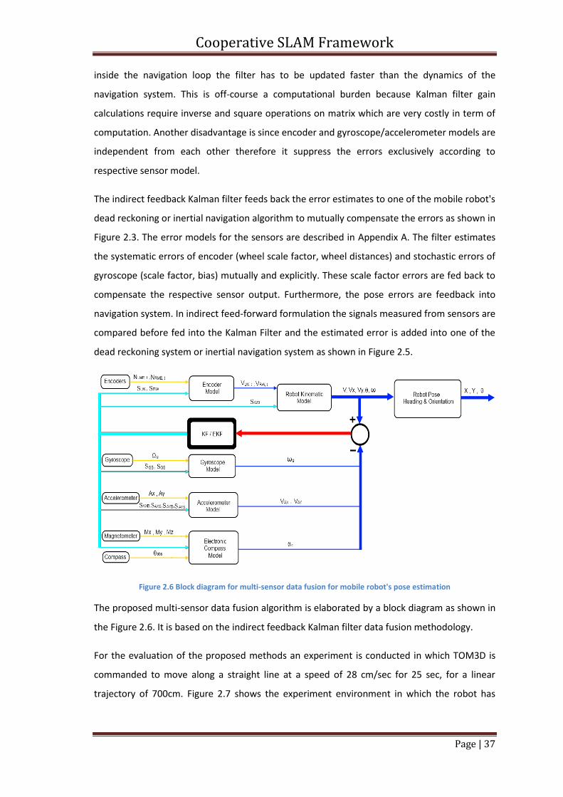
Cooperative SLAM Framework
Page | 37
inside the navigation loop the filter has to be updated faster than the dynamics of the
navigation system. This is off-course a computational burden because Kalman filter gain
calculations require inverse and square operations on matrix which are very costly in term of
computation. Another disadvantage is since encoder and gyroscope/accelerometer models are
independent from each other therefore it suppress the errors exclusively according to
respective sensor model.
The indirect feedback Kalman filter feeds back the error estimates to one of the mobile robot's
dead reckoning or inertial navigation algorithm to mutually compensate the errors as shown in
Figure 2.3. The error models for the sensors are described in Appendix A. The filter estimates
the systematic errors of encoder (wheel scale factor, wheel distances) and stochastic errors of
gyroscope (scale factor, bias) mutually and explicitly. These scale factor errors are fed back to
compensate the respective sensor output. Furthermore, the pose errors are feedback into
navigation system. In indirect feed-forward formulation the signals measured from sensors are
compared before fed into the Kalman Filter and the estimated error is added into one of the
dead reckoning system or inertial navigation system as shown in Figure 2.5.
Figure 2.6 Block diagram for multi-sensor data fusion for mobile robot's pose estimation
The proposed multi-sensor data fusion algorithm is elaborated by a block diagram as shown in
the Figure 2.6. It is based on the indirect feedback Kalman filter data fusion methodology.
For the evaluation of the proposed methods an experiment is conducted in which TOM3D is
commanded to move along a straight line at a speed of 28 cm/sec for 25 sec, for a linear
trajectory of 700cm. Figure 2.7 shows the experiment environment in which the robot has
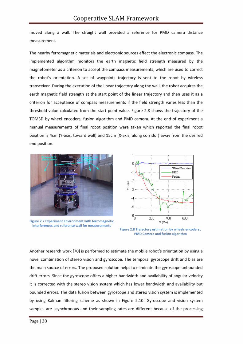
Cooperative SLAM Framework
Page | 38
moved along a wall. The straight wall provided a reference for PMD camera distance
measurement.
The nearby ferromagnetic materials and electronic sources effect the electronic compass. The
implemented algorithm monitors the earth magnetic field strength measured by the
magnetometer as a criterion to accept the compass measurements, which are used to correct
the robot’s orientation. A set of waypoints trajectory is sent to the robot by wireless
transceiver. During the execution of the linear trajectory along the wall, the robot acquires the
earth magnetic field strength at the start point of the linear trajectory and then uses it as a
criterion for acceptance of compass measurements if the field strength varies less than the
threshold value calculated from the start point value. Figure 2.8 shows the trajectory of the
TOM3D by wheel encoders, fusion algorithm and PMD camera. At the end of experiment a
manual measurements of final robot position were taken which reported the final robot
position is 4cm (Y-axis, toward wall) and 15cm (X-axis, along corridor) away from the desired
end position.
Figure 2.7 Experiment Environment with ferromagnetic interferences and reference wall for measurements
Figure 2.8 Trajectory estimation by wheels encoders , PMD Camera and fusion algorithm
Another research work [70] is performed to estimate the mobile robot’s orientation by using a
novel combination of stereo vision and gyroscope. The temporal gyroscope drift and bias are
the main source of errors. The proposed solution helps to eliminate the gyroscope unbounded
drift errors. Since the gyroscope offers a higher bandwidth and availability of angular velocity
it is corrected with the stereo vision system which has lower bandwidth and availability but
bounded errors. The data fusion between gyroscope and stereo vision system is implemented
by using Kalman filtering scheme as shown in Figure 2.10. Gyroscope and vision system
samples are asynchronous and their sampling rates are different because of the processing
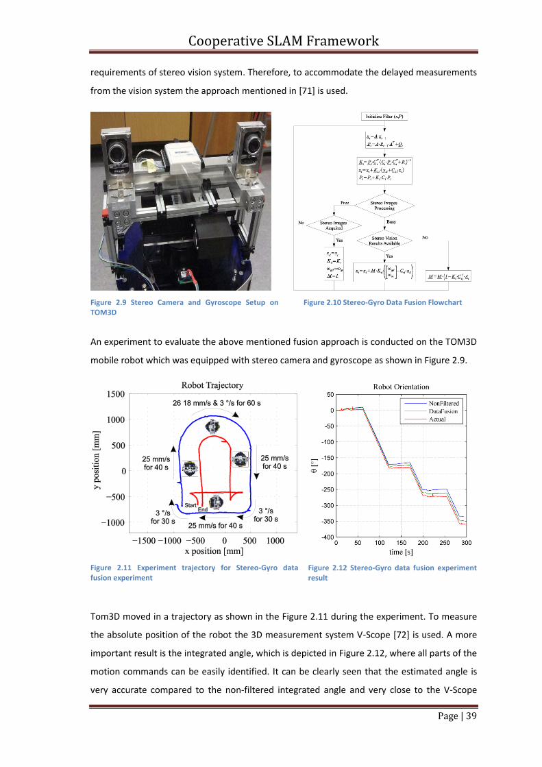
Cooperative SLAM Framework
Page | 39
requirements of stereo vision system. Therefore, to accommodate the delayed measurements
from the vision system the approach mentioned in [71] is used.
Figure 2.9 Stereo Camera and Gyroscope Setup on TOM3D
Figure 2.10 Stereo-Gyro Data Fusion Flowchart
An experiment to evaluate the above mentioned fusion approach is conducted on the TOM3D
mobile robot which was equipped with stereo camera and gyroscope as shown in Figure 2.9.
Figure 2.11 Experiment trajectory for Stereo-Gyro data fusion experiment
Figure 2.12 Stereo-Gyro data fusion experiment result
Tom3D moved in a trajectory as shown in the Figure 2.11 during the experiment. To measure
the absolute position of the robot the 3D measurement system V-Scope [72] is used. A more
important result is the integrated angle, which is depicted in Figure 2.12, where all parts of the
motion commands can be easily identified. It can be clearly seen that the estimated angle is
very accurate compared to the non-filtered integrated angle and very close to the V-Scope
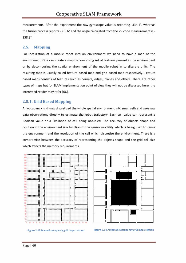
Cooperative SLAM Framework
Page | 40
measurements. After the experiment the raw gyroscope value is reporting -334.1°, whereas
the fusion process reports -355.6° and the angle calculated from the V-Scope measurement is -
358.3°.
2.5. Mapping
For localization of a mobile robot into an environment we need to have a map of the
environment. One can create a map by composing set of features present in the environment
or by decomposing the spatial environment of the mobile robot in to discrete units. The
resulting map is usually called feature based map and grid based map respectively. Feature
based maps consists of features such as corners, edges, planes and others. There are other
types of maps but for SLAM implementation point of view they will not be discussed here, the
interested reader may refer [66].
2.5.1. Grid Based Mapping
An occupancy grid map discretized the whole spatial environment into small cells and uses raw
data observations directly to estimate the robot trajectory. Each cell value can represent a
Boolean value or a likelihood of cell being occupied. The accuracy of objects shape and
position in the environment is a function of the sensor modality which is being used to sense
the environment and the resolution of the cell which discretize the environment. There is a
compromise between the accuracy of representing the objects shape and the grid cell size
which affects the memory requirements.
Figure 2.13 Manual occupancy grid map creation
Figure 2.14 Automatic occupancy grid map creation
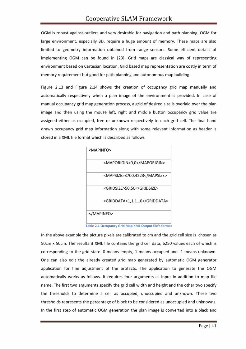
Cooperative SLAM Framework
Page | 41
OGM is robust against outliers and very desirable for navigation and path planning. OGM for
large environment, especially 3D, require a huge amount of memory. These maps are also
limited to geometry information obtained from range sensors. Some efficient details of
implementing OGM can be found in [23]. Grid maps are classical way of representing
environment based on Cartesian location. Grid based map representation are costly in term of
memory requirement but good for path planning and autonomous map building.
Figure 2.13 and Figure 2.14 shows the creation of occupancy grid map manually and
automatically respectively when a plan image of the environment is provided. In case of
manual occupancy grid map generation process, a grid of desired size is overlaid over the plan
image and then using the mouse left, right and middle button occupancy grid value are
assigned either as occupied, free or unknown respectively to each grid cell. The final hand
drawn occupancy grid map information along with some relevant information as header is
stored in a XML file format which is described as follows
<MAPINFO>
<MAPORIGIN>0,0</MAPORIGIN>
<MAPSIZE>3700,4223</MAPSIZE>
<GRIDSIZE>50,50</GRIDSIZE>
<GRIDDATA>1,1,1…0</GRIDDATA>
</MAPINFO>
Table 2.1 Occupancy Grid Map XML Output file's format
In the above example the picture pixels are calibrated to cm and the grid cell size is chosen as
50cm x 50cm. The resultant XML file contains the grid cell data, 6250 values each of which is
corresponding to the grid state. 0 means empty, 1 means occupied and -1 means unknown.
One can also edit the already created grid map generated by automatic OGM generator
application for fine adjustment of the artifacts. The application to generate the OGM
automatically works as follows. It requires four arguments as input in addition to map file
name. The first two arguments specify the grid cell width and height and the other two specify
the thresholds to determine a cell as occupied, unoccupied and unknown. These two
thresholds represents the percentage of block to be considered as unoccupied and unknowns.
In the first step of automatic OGM generation the plan image is converted into a black and
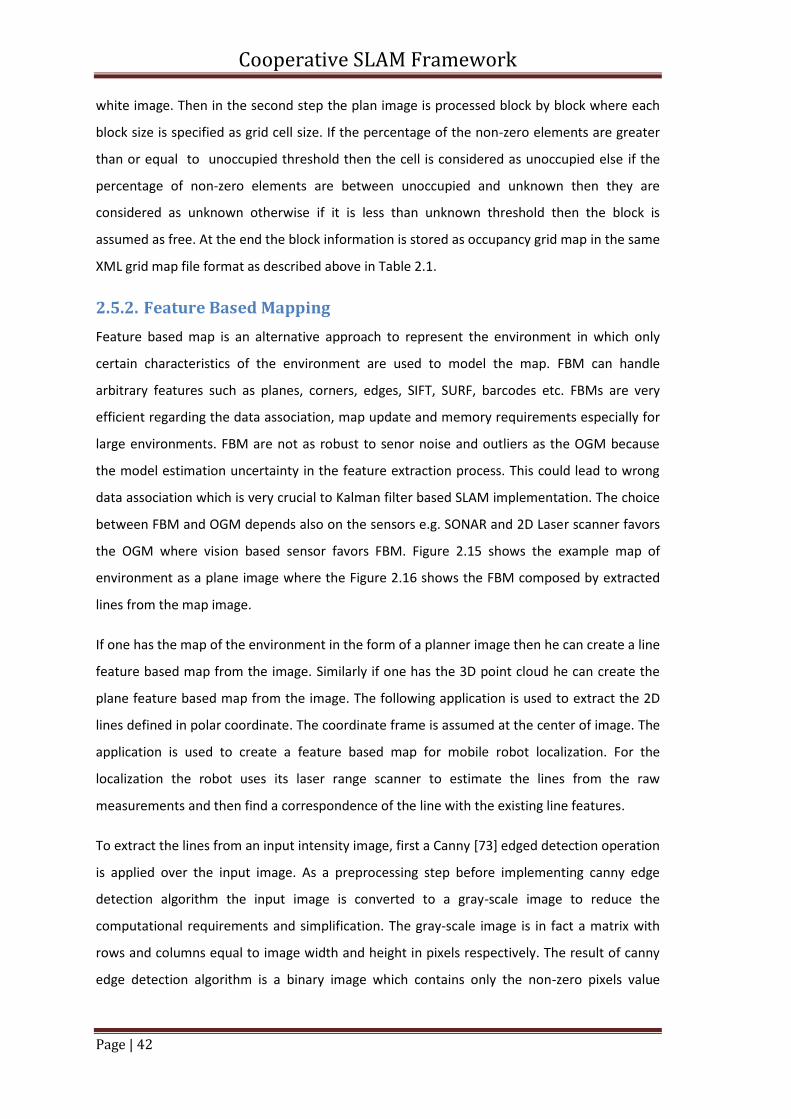
Cooperative SLAM Framework
Page | 42
white image. Then in the second step the plan image is processed block by block where each
block size is specified as grid cell size. If the percentage of the non-zero elements are greater
than or equal to unoccupied threshold then the cell is considered as unoccupied else if the
percentage of non-zero elements are between unoccupied and unknown then they are
considered as unknown otherwise if it is less than unknown threshold then the block is
assumed as free. At the end the block information is stored as occupancy grid map in the same
XML grid map file format as described above in Table 2.1.
2.5.2. Feature Based Mapping
Feature based map is an alternative approach to represent the environment in which only
certain characteristics of the environment are used to model the map. FBM can handle
arbitrary features such as planes, corners, edges, SIFT, SURF, barcodes etc. FBMs are very
efficient regarding the data association, map update and memory requirements especially for
large environments. FBM are not as robust to senor noise and outliers as the OGM because
the model estimation uncertainty in the feature extraction process. This could lead to wrong
data association which is very crucial to Kalman filter based SLAM implementation. The choice
between FBM and OGM depends also on the sensors e.g. SONAR and 2D Laser scanner favors
the OGM where vision based sensor favors FBM. Figure 2.15 shows the example map of
environment as a plane image where the Figure 2.16 shows the FBM composed by extracted
lines from the map image.
If one has the map of the environment in the form of a planner image then he can create a line
feature based map from the image. Similarly if one has the 3D point cloud he can create the
plane feature based map from the image. The following application is used to extract the 2D
lines defined in polar coordinate. The coordinate frame is assumed at the center of image. The
application is used to create a feature based map for mobile robot localization. For the
localization the robot uses its laser range scanner to estimate the lines from the raw
measurements and then find a correspondence of the line with the existing line features.
To extract the lines from an input intensity image, first a Canny [73] edged detection operation
is applied over the input image. As a preprocessing step before implementing canny edge
detection algorithm the input image is converted to a gray-scale image to reduce the
computational requirements and simplification. The gray-scale image is in fact a matrix with
rows and columns equal to image width and height in pixels respectively. The result of canny
edge detection algorithm is a binary image which contains only the non-zero pixels value
Cooperative SLAM Framework
Page | 43
corresponding to edges i.e. sudden changes in the image contrast. The canny algorithm
consists of the following four steps:
Figure 2.15 Original map image of the environment
Figure 2.16 Extracted line features from the map image
Step 1: Gaussian filter is applied to remove the noise. The filter consists of a kernel or mask, a
matrix, with a certain standard deviation. The resulting image is a blurred image which is a
result of convolving or sliding the kernel across the gray-scale image from left to right starting
from top to bottom.
Step 2: Since the edges are the gradient in the intensity of the image. The magnitude and
direction of the gradient for each pixel in the smoothed image is determined using Sobel [74]
technique. To get the edge intensity and direction, Sobel technique determines components of
the gradient along the x and y axis by convolving a 3x3 X-kernel and Y-kernel respectively with
the intensity image. The gradient magnitude is determined by using Euclidean distance
measure. Manhattan distance measure can be used to reduce computational complexity. The
gradient direction is calculated by using arctangent function.
Step 3: The edges which are found in the previous step are thick; therefore, they must be
narrowed. To thin down the thickness of edges the following algorithm is applied. Since there
Cooperative SLAM Framework
Page | 44
are eight neighboring pixels of any pixels except the border pixels, therefore the gradient
orientation is divided into eight regions of 45 each. The decision to keep the pixel gradient
value is based on the following condition. If the gradient value of the current pixel is greater
than the gradient values of the pixel in gradient direction and opposite of gradient direction
then its value is kept otherwise set to zero.
Step 4: The edges found in the image may be the true edges or it may be formed because of
the noise or rough surface. Usually fake edges are short, disconnected and irregular.
Distinction between true and fake edges can be made using thresholding. Using a single
threshold short discontinuous edges are formed because of the noise in the discontinuous
region. The canny edge detection algorithm discerns between true and fake edges using two
thresholds T1 and T2. If the gradient intensity is above T1 it is considered as strong edge.
Strong edges can be treated as true edge because it is unlikely to be caused by noise. If the
magnitude of the gradient is between T1 and T2 it is considered as weak edge otherwise
discarded. The weak edges may be true edges or because of color variation or noise. The weak
edge is considered as the true edge only if it is connected with a strong edge otherwise
discarded. Because if a weak an edge is connected with a true edge, it is likely to be a true
edge but because of the noise it is suppressed and considered as weak edge. Where the
disconnected weak edges are likely due to color variation or noise and therefore they are
independent of the strong edges thus discarded. The Tracking of weak edges adjency with
strong edges can be checked using Grass-fire, flood-fill, algorithm.
After the edge detection probabilistic Hough transformation is applied over the binary image.
Each non zero pixel in the image space is used for voting phase in Hough space. The voting
phase is also known as Hough transformation. The Hough space or accumulator is the
discretization of line's parameters space, i.e. a 2D space where each axis correspond to a
parameters of the line equation. Since one point can corresponds to many lines, therefore,
one point in image space corresponds to many points in the Hough space. Similarly, one line
can have correspondence with many points; therefore, each point in Hough space corresponds
to many points into the image space. To reduce the computation requirements in standard
Hough transformation, probabilistic Hough transformation uses two random non zero points
to form a line which vote for a point in Hough space. After a certain number of iterations the
Hough space points above a certain thresholds are treated as lines. The corresponding
endpoints of the line are then extracted from the image space. The extracted line segments
parameters and along with the line segment’s end points are stored in a XML file format
Cooperative SLAM Framework
Page | 45
which later can be retrieved by the localization module during the loading of the map at
startup.
2.5.2.1 Plane Extraction and Map Building Using a Kinect Equipped Mobile Robot
3D Map building is fundamental to the autonomous navigation of the mobile robots in real
world environment. Furthermore it could help mobile robots to reason about environment.
State of the art mobile robots use 3D range scanning devices such as laser scanner, time of
flight cameras, stereo cameras and RGB-D cameras to sense the spatial environment and
construct the map from acquired point clouds. Traditional computer vision solutions to
construct 3D maps from multi-view videos or related images are computational resource
demanding and time consuming. Geometric features such as lines and planes are prevalent
into the manmade environments such as offices and factory floors. Mobile robots can use such
geometric features to construct a map for collision free autonomous navigation and
localization in such environments.
This research work uses the plane detection algorithms to detect the planes from the raw
Kinect data and registers them using octree data structure. During this experiment a geometric
feature (3D plane) based map is created using a differential drive mobile robot equipped with
a Microsoft Kinect camera in an indoor office environment as shown in Figure 2.17. To create
the model of the environment several scans have to be fused. The fusing process is easy if the
position of the scanner is known otherwise scan registrations have to be performed to
estimate the pose of the scanner. This experiment does not concentrate on the scan
registration process. It is also assumed that the mobile robot has been already localized thus
an accurate mobile robot pose is available for mapping.
Kinect is an inexpensive RGB-D camera which provides a color image stream and a depth
image stream in an indoor environment in real time which can be very useful for dense 3D
color mapping in cluttered indoor environments. Despite of the impressive acquisition rate the
raw data is unsuitable for navigation and real-time 3D mapping because of the enormous
amount of the data to be processed. Therefore, geometric features such as planes are
extracted from the raw 3D point clouds.
Since Kinect sensor acquires enormous amounts of data, 9.2 million 3D points in one sec, it is
challenging to process the data in real time because of the limited amount of computation
resources available on mobile robots, furthermore, raw 3D point clouds from Kinect sensor are
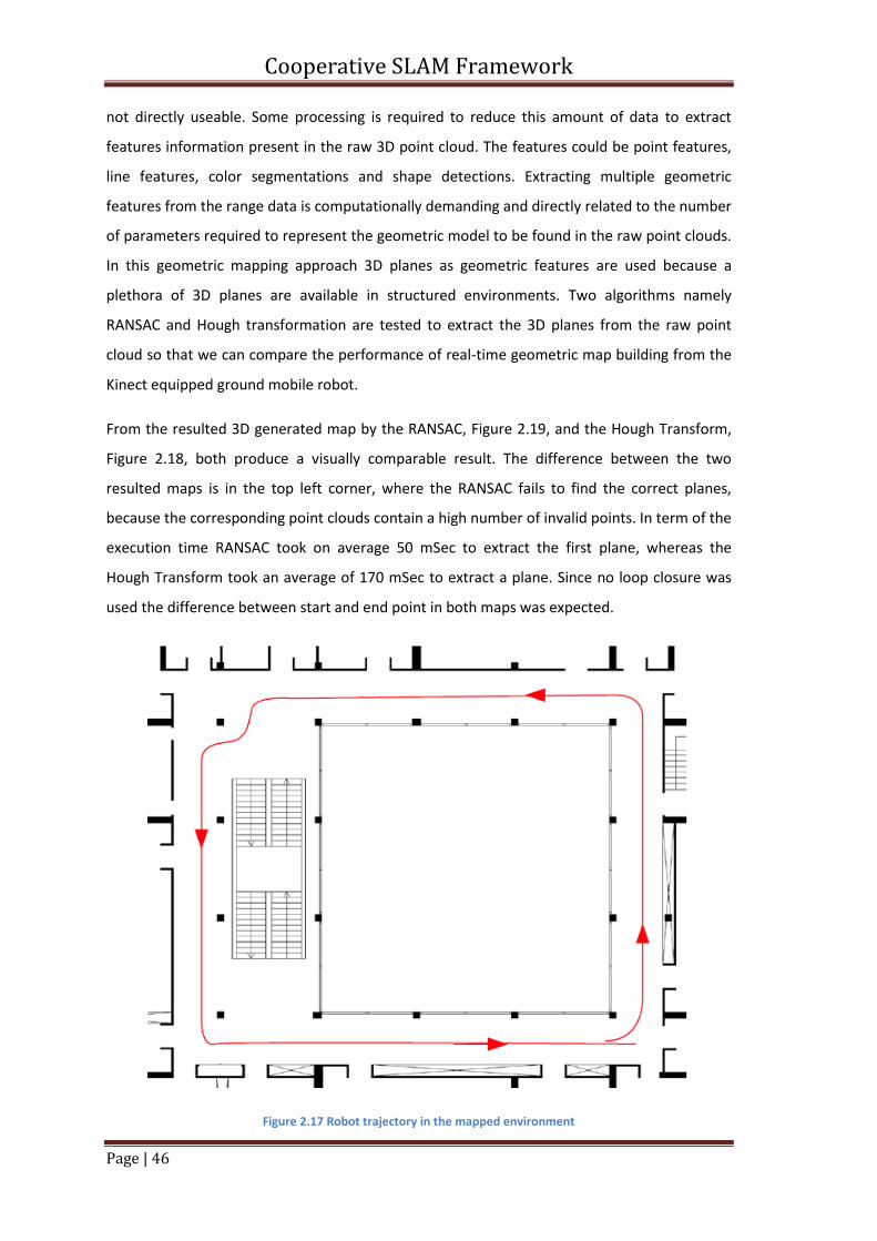
Cooperative SLAM Framework
Page | 46
not directly useable. Some processing is required to reduce this amount of data to extract
features information present in the raw 3D point cloud. The features could be point features,
line features, color segmentations and shape detections. Extracting multiple geometric
features from the range data is computationally demanding and directly related to the number
of parameters required to represent the geometric model to be found in the raw point clouds.
In this geometric mapping approach 3D planes as geometric features are used because a
plethora of 3D planes are available in structured environments. Two algorithms namely
RANSAC and Hough transformation are tested to extract the 3D planes from the raw point
cloud so that we can compare the performance of real-time geometric map building from the
Kinect equipped ground mobile robot.
From the resulted 3D generated map by the RANSAC, Figure 2.19, and the Hough Transform,
Figure 2.18, both produce a visually comparable result. The difference between the two
resulted maps is in the top left corner, where the RANSAC fails to find the correct planes,
because the corresponding point clouds contain a high number of invalid points. In term of the
execution time RANSAC took on average 50 mSec to extract the first plane, whereas the
Hough Transform took an average of 170 mSec to extract a plane. Since no loop closure was
used the difference between start and end point in both maps was expected.
Figure 2.17 Robot trajectory in the mapped environment
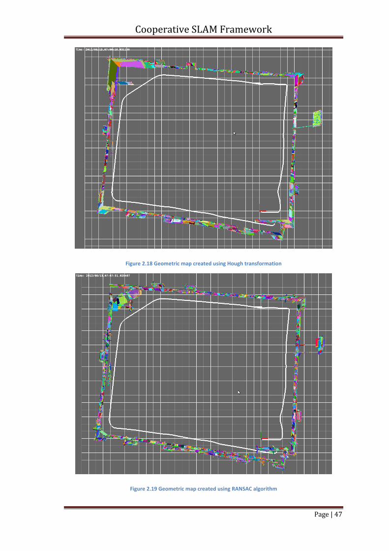
Cooperative SLAM Framework
Page | 47
Figure 2.18 Geometric map created using Hough transformation
Figure 2.19 Geometric map created using RANSAC algorithm
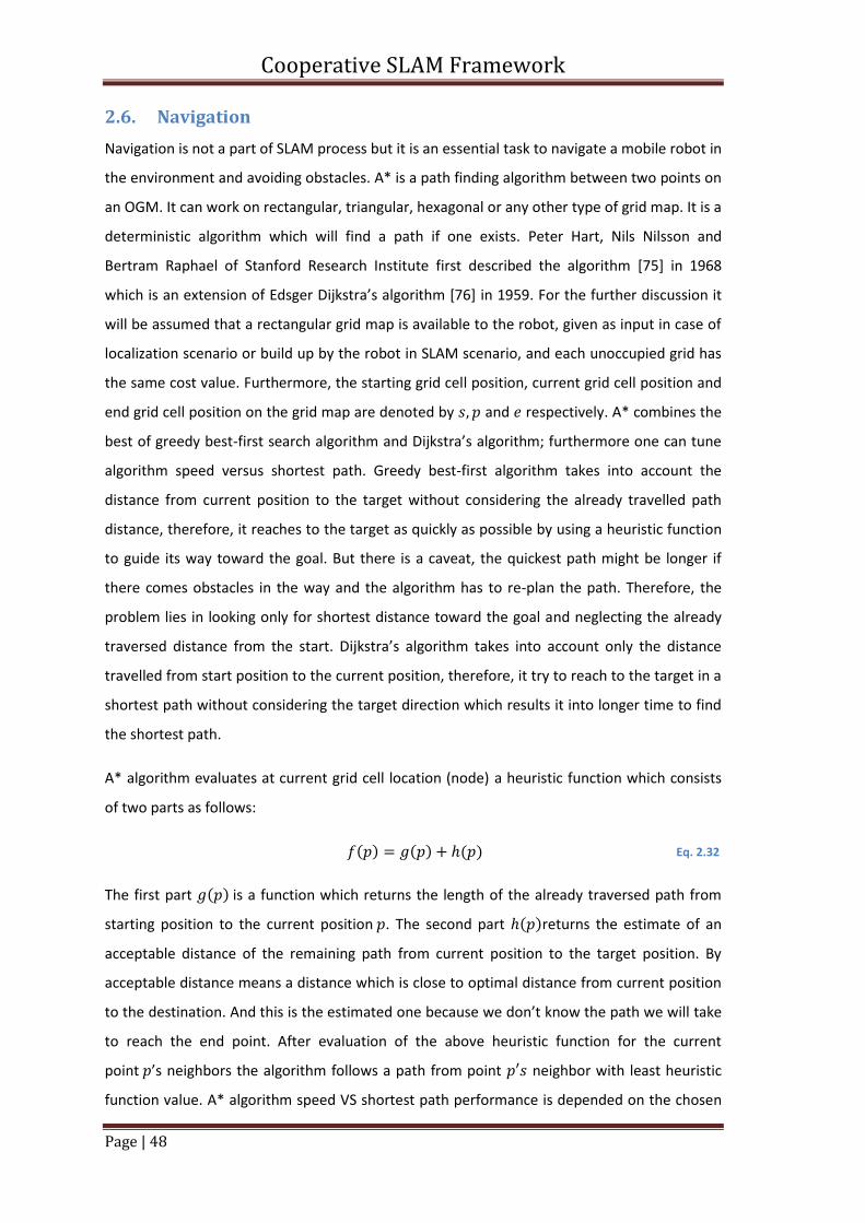
Cooperative SLAM Framework
Page | 48
2.6. Navigation
Navigation is not a part of SLAM process but it is an essential task to navigate a mobile robot in
the environment and avoiding obstacles. A* is a path finding algorithm between two points on
an OGM. It can work on rectangular, triangular, hexagonal or any other type of grid map. It is a
deterministic algorithm which will find a path if one exists. Peter Hart, Nils Nilsson and
Bertram Raphael of Stanford Research Institute first described the algorithm [75] in 1968
which is an extension of Edsger Dijkstra’s algorithm [76] in 1959. For the further discussion it
will be assumed that a rectangular grid map is available to the robot, given as input in case of
localization scenario or build up by the robot in SLAM scenario, and each unoccupied grid has
the same cost value. Furthermore, the starting grid cell position, current grid cell position and
end grid cell position on the grid map are denoted by and respectively. A* combines the
best of greedy best-first search algorithm and Dijkstra’s algorithm; furthermore one can tune
algorithm speed versus shortest path. Greedy best-first algorithm takes into account the
distance from current position to the target without considering the already travelled path
distance, therefore, it reaches to the target as quickly as possible by using a heuristic function
to guide its way toward the goal. But there is a caveat, the quickest path might be longer if
there comes obstacles in the way and the algorithm has to re-plan the path. Therefore, the
problem lies in looking only for shortest distance toward the goal and neglecting the already
traversed distance from the start. Dijkstra’s algorithm takes into account only the distance
travelled from start position to the current position, therefore, it try to reach to the target in a
shortest path without considering the target direction which results it into longer time to find
the shortest path.
A* algorithm evaluates at current grid cell location (node) a heuristic function which consists
of two parts as follows:
( ) ( ) ( ) Eq. 2.32
The first part ( ) is a function which returns the length of the already traversed path from
starting position to the current position . The second part ( )returns the estimate of an
acceptable distance of the remaining path from current position to the target position. By
acceptable distance means a distance which is close to optimal distance from current position
to the destination. And this is the estimated one because we don’t know the path we will take
to reach the end point. After evaluation of the above heuristic function for the current
point ’s neighbors the algorithm follows a path from point neighbor with least heuristic
function value. A* algorithm speed VS shortest path performance is depended on the chosen
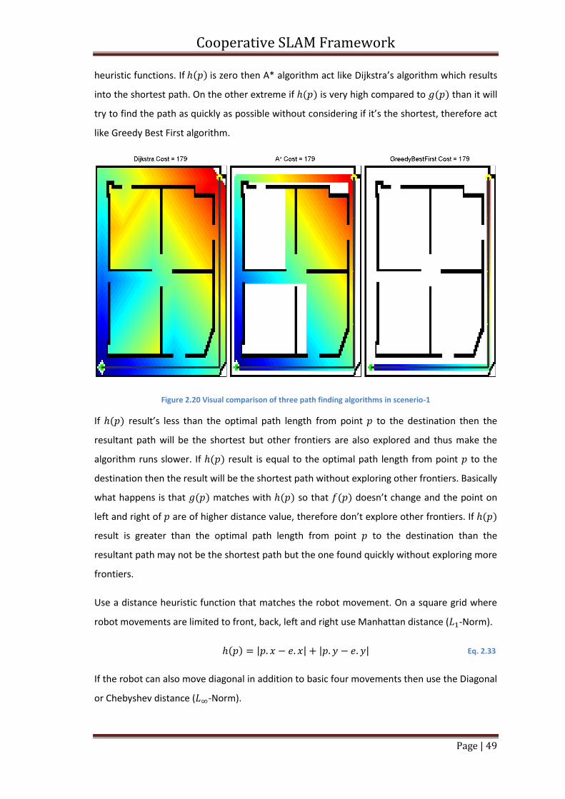
Cooperative SLAM Framework
Page | 49
heuristic functions. If ( ) is zero then A* algorithm act like Dijkstra’s algorithm which results
into the shortest path. On the other extreme if ( ) is very high compared to ( ) than it will
try to find the path as quickly as possible without considering if it’s the shortest, therefore act
like Greedy Best First algorithm.
Figure 2.20 Visual comparison of three path finding algorithms in scenerio-1
If ( ) result’s less than the optimal path length from point to the destination then the
resultant path will be the shortest but other frontiers are also explored and thus make the
algorithm runs slower. If ( ) result is equal to the optimal path length from point to the
destination then the result will be the shortest path without exploring other frontiers. Basically
what happens is that ( ) matches with ( ) so that ( ) doesn’t change and the point on
left and right of are of higher distance value, therefore don’t explore other frontiers. If ( )
result is greater than the optimal path length from point to the destination than the
resultant path may not be the shortest path but the one found quickly without exploring more
frontiers.
Use a distance heuristic function that matches the robot movement. On a square grid where
robot movements are limited to front, back, left and right use Manhattan distance ( -Norm).
( ) | | | | Eq. 2.33
If the robot can also move diagonal in addition to basic four movements then use the Diagonal
or Chebyshev distance ( -Norm).
Cooperative SLAM Framework
Page | 50
Figure 2.21 Visual comparison of three path finding algorithms in scenerio-2
( ) (| | | |) Eq. 2.34
If the robot can maneuvers in any direction then use the Euclidean distance ( -Norm). One
caveat to the Euclidean distance heuristic is that it takes longer to run the A* algorithm to find
the shortest path because ( ) will be smaller than ( ). The Euclidean distance calculated by
( ) is always smaller than the Manhattan or Chebyshev distance calculated by ( ).
( ) √( ) ( ) Eq. 2.35
If there are multiple end locations of same priority then A* algorithm can reach any one of the
location by the following modification. Instead of evaluating the ( ), evaluate
( ( ) ( )) while rest of the algorithm remains the same.
The performance of the A* algorithm also depends on one of the important detail i.e. in case
of the different frontiers of the same value which one to choose, there are different
strategies which produces different results. One approach is to choose the point with lowest
value. Another approach is to calculate the magnitude of the cross product between vectors
formed from start point to end point and from the frontier point to the end point and
selecting the frontier with smaller resultant area.
Figure 2.20 and Figure 2.21 show the visual comparison of the three above mentioned
navigation algorithm with same starting position while different end position. The colored
gradient visually depicts the cost of reaching at that point. From Figure 2.20 it seems that
Cooperative SLAM Framework
Page | 51
Greedy Best First algorithm is the best but one can see from Figure 2.21 that it traps within the
obstacles and even the found path which is shown by thick bold line is not the shortest. Where
the Dijkstra’s algorithm always find the shortest path if one exists but it will take longer to
execute because it searches the path in all direction from the starting point.
2.6.1. Implementation
The A* algorithm uses priority list for its implementation. A priority list is an data structure
where each element stored has a priority value attached to it and when a data value is asked
from the priority list then the data value with the highest priority is returned. Each grid cell is
called a node in A* implementation. A node consists of following variables; grid cell location,
grid cell state (Occupied, Unoccupied), a pointer to parent node and variables for storing
and value. There are two lists maintained by the algorithm, let’s call them FRONTIERS and
VISITED. A FRONTIER is a priority list which contains the nodes that are the valid candidates for
examining. The value is used as the priority value of the FRONTIERS priority list. When the
FRONTIERS list is queried then the node with minimum value shall be returned. A VISITED list
contains nodes which have been already examined; they are the interior of the frontiers cells.
In the beginning both lists are empty; to start the algorithm the starting node is added to the
FRONTIERS list. Then we start our search loop. A node from the FRONTIERS list is queried
which is called current node. If the current node matches to the destination node then we add
the current node to our resultant path list and backtrack all the nodes using the parent field of
the nodes in the VISITED list until we reach to the starting node. Otherwise the current node is
added to the VISITED list. The neighboring nodes, 8 in 2D or 26 in 3D, to the current node are
examined; the nodes which are un-occupied and already not in the FRONTIERS or VISITED list,
there and value are calculated and their parents field is set as current node and then
added to the FRONTIERS list. The h value is calculated using the chosen heuristic value the
value is the sum of current nodes value plus moving cost from current node to the
neighboring node. Then re-query the updated FRONTIERS list for the next current node. This
process is repeated until there are no more nodes in the frontiers, in that case no path exists,
or the destination node matches the current node which means the path is found.
Cooperative SLAM Framework
Page | 52
2.7. Summary
In this chapter the background concepts related to mobile robot SLAM and navigation are
discussed. First of all the probabilistic motion model for differential drive robots and range
sensor models are discussed.
Then a Kalman filter and particle filter based probabilistic estimation techniques are
introduced which are the core part of SLAM solution.
Afterwards the data fusion strategies are discussed which are used for the accurate mobile
robot pose estimation.
Both the grid based map and feature based map construction process are discussed which
directly affect the SLAM algorithm implementation.
And finally A* navigation algorithm is discussed which is very important for the autonomous
mobile robot navigation.
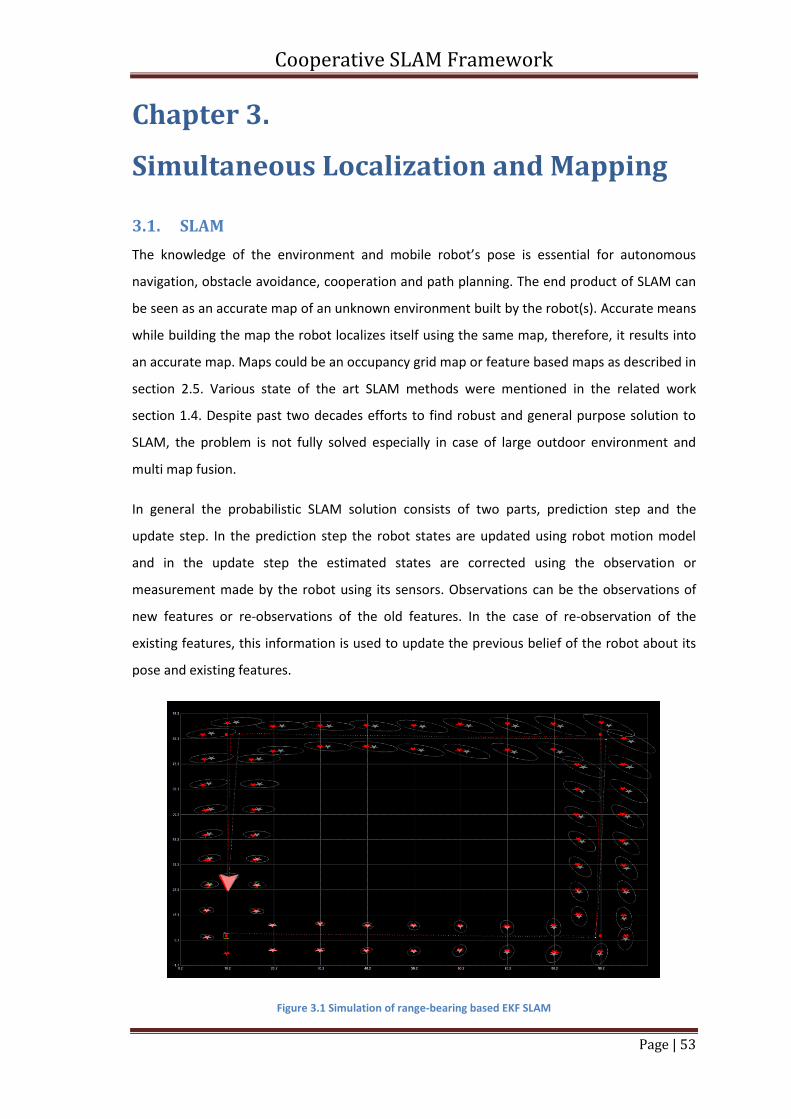
Cooperative SLAM Framework
Page | 53
Chapter 3.
Simultaneous Localization and Mapping
3.1. SLAM
The knowledge of the environment and mobile robot’s pose is essential for autonomous
navigation, obstacle avoidance, cooperation and path planning. The end product of SLAM can
be seen as an accurate map of an unknown environment built by the robot(s). Accurate means
while building the map the robot localizes itself using the same map, therefore, it results into
an accurate map. Maps could be an occupancy grid map or feature based maps as described in
section 2.5. Various state of the art SLAM methods were mentioned in the related work
section 1.4. Despite past two decades efforts to find robust and general purpose solution to
SLAM, the problem is not fully solved especially in case of large outdoor environment and
multi map fusion.
In general the probabilistic SLAM solution consists of two parts, prediction step and the
update step. In the prediction step the robot states are updated using robot motion model
and in the update step the estimated states are corrected using the observation or
measurement made by the robot using its sensors. Observations can be the observations of
new features or re-observations of the old features. In the case of re-observation of the
existing features, this information is used to update the previous belief of the robot about its
pose and existing features.
Figure 3.1 Simulation of range-bearing based EKF SLAM
Cooperative SLAM Framework
Page | 54
Figure 3.1 displays the result of an EKF based Range-Bearing SLAM algorithm for known data
association. The robot’s pose uncertainty, shown by ellipse, increases as it moves as shown in
the above figure. In the simulation shown above, fig. 3.1, the robot moves inside a cloister.
The red stars represent the columns of the cloister which can be detected by a factitious
Range-Bearing sensor system mounted on the robot. The factitious sensor can provide the
range and bearing of the column with respect to the robot pose with some uncertainty in the
measured range and bearing. These columns can be considered as landmarks or point
features. The factitious robot sensor can also determine the unique ID printed on the column
for resolving the problem of data association or ambiguity among the same columns. The
small red squares represent the waypoints which the robot has to traverse. The red dotted
line represents the nominal trajectory of the robot while the gray dotted line represents the
estimated trajectory of the robot. The grey dotted ellipse represents the uncertainty in the
position. Two important results can be seen. First the gray stars represent the map generated
by the robot and the second is the robot pose uncertainty which never grows unbounded
because it uses the map to localize itself.
SLAM algorithms can be roughly classified by their estimation techniques and their map
representation. This chapter discusses the implementation of an EKF based SLAM algorithm.
The strength and weaknesses of the map representation have been discussed in section 2.5.
EKF is used as estimation engine for robot pose and features position estimation. The EKF
maintains and updates the mean and covariance of the states at each time step. The state
vector consist of robot pose and set of features parameters which are considered as
map
0 1 Eq. 3.1
Where the covariance matrix is as follows
[
] Eq. 3.2
The EKF-SLAM consists of two phases’ prediction and correction.
3.2. Prediction
The prediction phase estimates the robot pose and the map after the robot has executed a
motion command or when motion data is available from odometry. The map or set of
landmarks are assumed to be constant or time invariant, therefore
Cooperative SLAM Framework
Page | 55
0 ( )
1 Eq. 3.3
The kinematic motion model ( ) of the differential drive robot to estimate the pose
states is as follows:
( )
[ (
) (
)
(
) (
)
( ) ]
Eq. 3.4
Where ( ) is the current robot pose, ( )
is the odometry inputs
which consist of linear and angular distance measured by the robot wheel encoders. Here it is
assumed that the robot pose error is due to the non-systematic errors because of robot wheel
slip and interaction of the wheel with the ground. These errors . ( ) (
)
( )/
are assumed to have a normal or Gaussian distribution and they are un-correlated.
The systematic errors such as due to difference of left and right wheel diameters and
difference of wheel base length from the nominal value are also assumed to be corrected by
the odometry calibration procedure such as UMBmark [60].
After estimating the state vector as a result of robot motion, the uncertainty of the robot and
map features states are calculated as follows:
[
] *
+ Eq. 3.5
Where are the new robot and map uncertainties and is the cross covariance
between robot and map features. are the old robot uncertainties. It
can be seen from above equation that the uncertainty of the robot pose is propogated
from the previous robot state uncertainty in addition to the uncertainty due to the noise. The
uncertainty of the map features remain the same but the covariance between the
robot and map feature changes. Where and are the Jacobians of the robot motion model
with respect the pose vector and noise vector. These Jacobians have the following values
Cooperative SLAM Framework
Page | 56
( ) [
.
/
.
/
] Eq. 3.6
( ) [
] Eq. 3.7
In Eq. 3.5 is the covariance matrix of the non-systematic errors which is defined as follows:
[
] Eq. 3.8
3.3. Correction
The correction phase of the EKF based SLAM algorithm is very complex. It consists of
clustering, feature extraction, expected feature prediction, map update and mapping new
features. Each of these steps is described in details as follows.
3.3.1. Clustering or Segmentation
Segmentation is usually the first step after range sensor data acquisition, sometime it is
followed by filtering. The real depth data from range measurement sensors contains more
than one geometric model or features present in the real environment, therefore, as a
preprocessing step to feature extraction clustering or segmentation is performed.
Segmentation groups the related set of data so that the geometric model of the feature is
estimated from the range data segment.
The SICK PLS-101 laser-scanner is mounted on one of the robot, TOM3D. Because of the 2D
range scan measurements provided by the SICK laser scanner line features are selected for
performing SLAM. The laser-scanner has a CCW rotating mirror at 25 rpm (40msec/scan). It
uses time of flight principle by the help of a 3 GHz counter [77] which results into range
measurement accuracy of 5cm. The angular resolution of the laser scanner is 0.5° and the
measurement range is from 7cm to 50m. During first half of 40msec interval the range
measurement in a semicircle is done while during the next 20msec the mirror is rotated back.
From the maximum linear (V) and angular (W) velocity the distance and angle traversed by the
robot can be calculated. For our robots the V=0.5m/sec and W=10°/sec results into =1cm
and =0.2° which is negligible compared to measurement error therefore, we can neglect
the measurement delay during the robot motion.
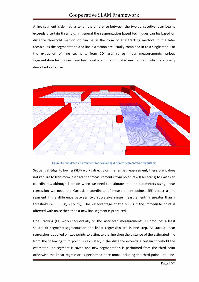
Cooperative SLAM Framework
Page | 57
A line segment is defined as when the difference between the two consecutive laser beams
exceeds a certain threshold. In general the segmentation based techniques can be based on
distance threshold method or can be in the form of line tracking method. In the later
techniques the segmentation and line extraction are usually combined in to a single step. For
the extraction of line segments from 2D laser range finder measurements various
segmentation techniques have been evaluated in a simulated environment, which are briefly
described as follows.
Figure 3.2 Simulated environment for evaluating different segmentation algorithms
Sequential Edge Following (SEF) works directly on the range measurement, therefore it does
not require to transform laser scanner measurements from polar (raw laser scans) to Cartesian
coordinates, although later on when we need to estimate the line parameters using linear
regression we need the Cartesian coordinate of measurement points. SEF detect a line
segment if the difference between two successive range measurements is greater than a
threshold i.e. | | . One disadvantage of the SEF is if the immediate point is
affected with noise then then a new line segment is produced.
Line Tracking (LT) works sequentially on the laser scan measurements. LT produces a least
square fit segment; segmentation and linear regression are in one step. At start a linear
regression is applied on two points to estimate the line then the distance of the estimated line
from the following third point is calculated, if the distance exceeds a certain threshold the
estimated line segment is saved and new segmentation is performed from the third point
otherwise the linear regression is performed once more including the third point until line-
Cooperative SLAM Framework
Page | 58
point distance exceed for next point or all the points are processed. The same disadvantage of
distance threshold as in the case of SEF also applies to LT when the next point which decides
the break of line is disturbed by the noise. The next point bias the estimate more when the
linear regression set is smaller. Both SEF and LT depend on the distance of the point from the
laser scanner. SEF and LET can be improved by using previous and last point information into
account.
Iterative End Point Fit (IEPF) [78] is a recursive algorithm which is executed when all data
measurement points are available. As a pre-processing step it also requires the points to be
converted into Cartesian coordinates. Then a line is estimated from first and last point
afterward all the points’ distances from the line is calculated. In case when no distance exceed
a threshold this is the estimated line (or to enhance the parameters linear regression is
performed on the point sets) otherwise the point with the maximum distance is selected as
dividing point for two line segments which are again recursively checked iteratively for line-
point distance. SEF and LT algorithms are fast compared to IEPF where IEPF is robust in both
indoor and outdoor environments.
The decision to create cluster is based on a criteria ( ) where ( ) is a
Euclidean distance between two consecutive laser beam end points calculated by law of
cosine i.e.
( ) √
( ) Eq. 3.9
The distance can be approximated by the following equation because of the very small angles
among laser beams i.e. 0.5°
( ) | | Eq. 3.10
The important point in clustering is how to choose the threshold? Dietmayer [79] uses the
following threshold condition
( ) Eq. 3.11
Where is a constant used for noise handling and
√ ( ( )) ( )
Eq. 3.12
Cooperative SLAM Framework
Page | 59
The dependence of threshold on the range is because of radial measurement principle. Santos
[80] included the parameter aiming to reduce the dependence of the absolute distance of
the point from the laser-scanner.
( )
( ) . . / .
// Eq. 3.13
Lee [81] proposed a simple method for line segments extraction threshold
|
| Eq. 3.14
Kalman filter has also been used for segmentation process; interested reader may refer [82].
3.3.2. Feature Extraction
Features are distinguishable entities in mobile robot’s sensor data which provides valuable
information regarding the location of the mobile robot and mapping of the environment.
Features or landmarks correspond to physical objects in the mobile robot environment. They
bring different kind of information of environment objects into the map which helps the
mobile robot to navigate using that map. Furthermore, they compress the sensor data size by
modeling them into entities which constituted the map. This is a very important aspect of the
large scale environment. Features usually depend on the type of sensor being used for the
mobile robot e.g. for 2D laser range scanner the features could be lines, corner and circles, for
3D laser range scanner, TOF cameras or RGB-D cameras the features could be planes and for
vision sensors features can be such as SIFT [83] or SURF [84].
Geometric features such as corners, lines, circles, planes and cylinders are most common
features which are being used to model the environment from range sensor measurements.
The geometric features are estimated by fitting the range measurements to the mathematical
model of the feature. The literature on model fitting can be categorized into two broad
categories i.e. Clustering (Hough Transformation) and Least Square Methods. A general form
for the linear least square estimation process is shown in the Appendix B. During geometric
feature extraction process the measurements are compared with a geometric model such as
line or plane, the inliers are then used to estimate the parameters of the model. The
parameter estimation problem can be mathematically seen as an optimization problem
because of the over-determined system and measurement errors. One can use the least
square method, RANSAC or Hough transformation to estimate the single or multiple models
from the measurements. Two different types of geometric features for modeling the robot
Cooperative SLAM Framework
Page | 60
environment are used i.e. line and planes. The extracted features are then used in the feature
matching stage. A fitting function to a model must provide model parameters, error estimates
on the parameters and statistical measure of goodness-of-fit.
3.3.2.1 Probabilistic Line Extraction
Among many primitive 2D geometric features line features are the prevalent in structured
indoor environment. The Hessian normal form of line in polar coordinate is more desirable
because it doesn’t have the problem of representing lines parallel to x or y axis as in slope
intercepts form. This implicit representation also allows fast calculation of point to the line
distance. Least square estimation technique is used to estimate the parameters of a line from
the laser scanner measurement cluster. Least square estimation technique provides a
maximum likelihood estimation of the fitted parameters if the measurement errors are
independent and Gaussian. Weighted least square fitting is also known as chi-square fitting.
The sum of squares of weighted residual are called chi-square, i.e. the sum of square of normal
distributed quantities. Weighted least square line fitting is used to estimate the parameters of
a line if each laser beam has different error variance.
Laser range scanner takes measurements of the environment in polar coordinates
( ) during one scan. We defined the line in Hessian normal form as follows
( ) Eq. 3.15
Here is the shortest Euclidian distance of the line’s normal from the coordinate system’s
center and is its angle with abscissa. Since there is an uncertainty in each variable and
therefore we have to minimize the term on right hand side of the above equation. Each
variable can be represented as a random variable which has its own probability distribution
function. We assumed that both random variables measurements are independent,
furthermore, the PDF of both variables are Gaussian. The error of each
measurement ( ) can be specified by the minimum normal distance of the measurement
point and the line i.e. ( ) , from the estimated line ( ). This approach
results into a non-linear least square estimation which is computationally expensive to
compute but not results into a bias estimate. The parameters of the line can be found by
minimizing the sum square error of all the measurement points with respect to line
parameters i.e.
Cooperative SLAM Framework
Page | 61
∑
∑( ( ) )
Eq. 3.16
(∑( ( ) )
) Eq. 3.17
(∑( ( ) )
) Eq. 3.18
The above equations result into a non-linear least square estimation whose solution is
calculated in [85]. The parameters of line’s model in hessian normal form are calculated as
follows:
( ∑( )( )
∑( ) ( )
) Eq. 3.19
( ) ( ) Eq. 3.20
∑ ( )
Eq. 3.21
∑ ( )
Eq. 3.22
And the uncertainties of the line’s model parameters ( ) are because of the uncertainties in
measurements ( ) which are calculated using error propagation law in [85]. These
uncertainties are calculated as follows, assuming and
are independent and angular
uncertainties ( ) is negligible:
[
] Eq. 3.23
∑[
]
Eq. 3.24
∑[
]
Eq. 3.25
Cooperative SLAM Framework
Page | 62
∑[
]
Eq. 3.26
( ) ( )
Eq. 3.27
( )
( ) Eq. 3.28
∑∑( )( )
∑
Eq. 3.29
∑∑ ( )
∑
Eq. 3.30
Position correction and map construction process can be speedup by storing other information
regarding line segment such as direction vector (from one point to other), normal vector,
length of segment, number of points in line segments and its normal distance to origin.
3.3.2.2 Probabilistic Plane Extraction
State of the art mobile robots use 3D range scanning devices such as laser scanner, time of
flight cameras, stereo cameras and RGB-D cameras to sense the spatial environment and
construct the map from acquired point clouds. 3D Geometric features such as planes are
prevalent in the man-made environments such as offices and factory floors. Mobile robots can
use such geometric features to construct a map for collision free autonomous navigation and
localization in such environments. Various research works [86] [87] [88] [89] have been done
until now to extract the 3D planes from the point cloud data acquired from different range
sensor devices and build the 3D map of the environment. Asad [89] has proposed a mapping
system for mobile robots which used height maps created from range images for path
planning. Pathak [86] proposed a method for 3D mapping by a mobile robot, furthermore, his
proposed method utilizes the uncertainty of the plane parameters to compute the uncertainty
in the pose computed by scan registration. Weingarten et al. [88] proposed a method for
plane fitting for laser range scanner data and fuses matching planes together to find a
compact 3D model. Anderson et al. [90] uses an approach which fuses both color and range
information to detect 3D planes. Apart from various mapping algorithms for mobile robots
different sensors have also been used in combination with mapping algorithms to map 3D
environments. Such sensors include laser scanners [91], stereo vision and monocular cameras
[92] and time of flight camera [93]. A common approach for mapping is to align point clouds
Cooperative SLAM Framework
Page | 63
by finding rotation and translation between consecutive 3D scans [94]. Henry [95] maps the
environment using ICP and SIFT features. There exist numbers of other methods which extract
the 3D planes from the raw point clouds. Borrmann [96] uses the Hough transform to extract
the 3D plane from the raw point clouds. Triebel [97] uses expectation maximization, Gallo [98]
used RANSAC to extract the planes and Pathek [99] used the split and merge techniques to
detect the planes. In [100] two algorithms namely RANSAC and Hough transformation to
extract the 3D planes from the raw point cloud are tested to compare the performance of real-
time geometric map building from the Kinect equipped ground mobile robot. Recently most of
the research work also used Kinect camera. The work in [101] [102] [103] has focused on
extracted plane segmentation because of the sparsity, measurement range limitation and
occlusion of the measurements. These research works have used the color image to
complement the range limitation and sparsity of the depth measurement. The intensity
information can help in segmentation of the 3D point cloud data by detecting edges in the
intensity images corresponding to the area of interest in the 3D point cloud.
2D laser scanners are limited in use for mapping environments which contains simple
geometric shapes; furthermore the obstacles which are above or below the scanned planes
cannot be detected e.g. downward stairs. Where the stereo systems are dependent on lighting
conditions and cannot detect planes in homogenous regions. Kinect sensor has brought
acquiring colored 3D point clouds cheaper and quicker which in the past require expensive
time of flight cameras. Furthermore, to acquire colored point clouds the system consisting of
time of flight camera and image camera must be setup and calibrated but Kinect combines the
3D range finding capability and the color information. Since Kinect sensor acquires enormous
amounts of data, 9.2 million 3D points in one sec, it is challenging to process the data in real
time because of the limited amount of computation resources available on mobile robots,
furthermore, raw 3D point clouds from Kinect sensor are not directly useable. Extracting
multiple geometric features from the range data is computationally demanding and directly
related to the number of parameters required to represent the geometric model to be found
in the raw point clouds. In geometric mapping approach 3D planes can be used as geometric
features because a plethora of 3D planes are available in structured environments.
Hough transform is a well-known algorithm in computer vision society to detect multiple
models in the data compared to RANSAC which in its basic form assumes there is a single
model present in the data. It can detect lines, planes, spheres and other parameterizable
geometric objects in the input data. In spite of the robustness of the method against noisy
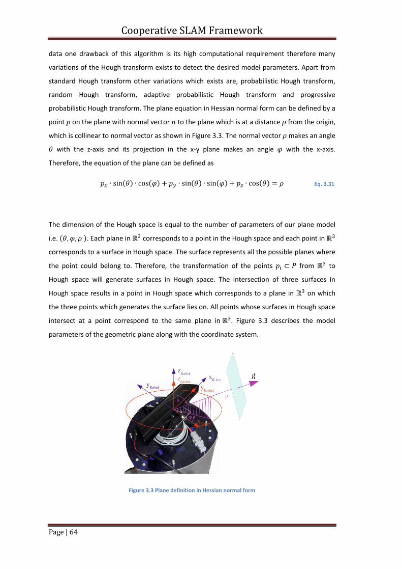
Cooperative SLAM Framework
Page | 64
data one drawback of this algorithm is its high computational requirement therefore many
variations of the Hough transform exists to detect the desired model parameters. Apart from
standard Hough transform other variations which exists are, probabilistic Hough transform,
random Hough transform, adaptive probabilistic Hough transform and progressive
probabilistic Hough transform. The plane equation in Hessian normal form can be defined by a
point on the plane with normal vector to the plane which is at a distance from the origin,
which is collinear to normal vector as shown in Figure 3.3. The normal vector makes an angle
with the z-axis and its projection in the x-y plane makes an angle with the x-axis.
Therefore, the equation of the plane can be defined as
( ) ( ) ( ) ( ) ( ) Eq. 3.31
The dimension of the Hough space is equal to the number of parameters of our plane model
i.e. ( ). Each plane in corresponds to a point in the Hough space and each point in
corresponds to a surface in Hough space. The surface represents all the possible planes where
the point could belong to. Therefore, the transformation of the points from to
Hough space will generate surfaces in Hough space. The intersection of three surfaces in
Hough space results in a point in Hough space which corresponds to a plane in on which
the three points which generates the surface lies on. All points whose surfaces in Hough space
intersect at a point correspond to the same plane in . Figure 3.3 describes the model
parameters of the geometric plane along with the coordinate system.
Figure 3.3 Plane definition in Hessian normal form
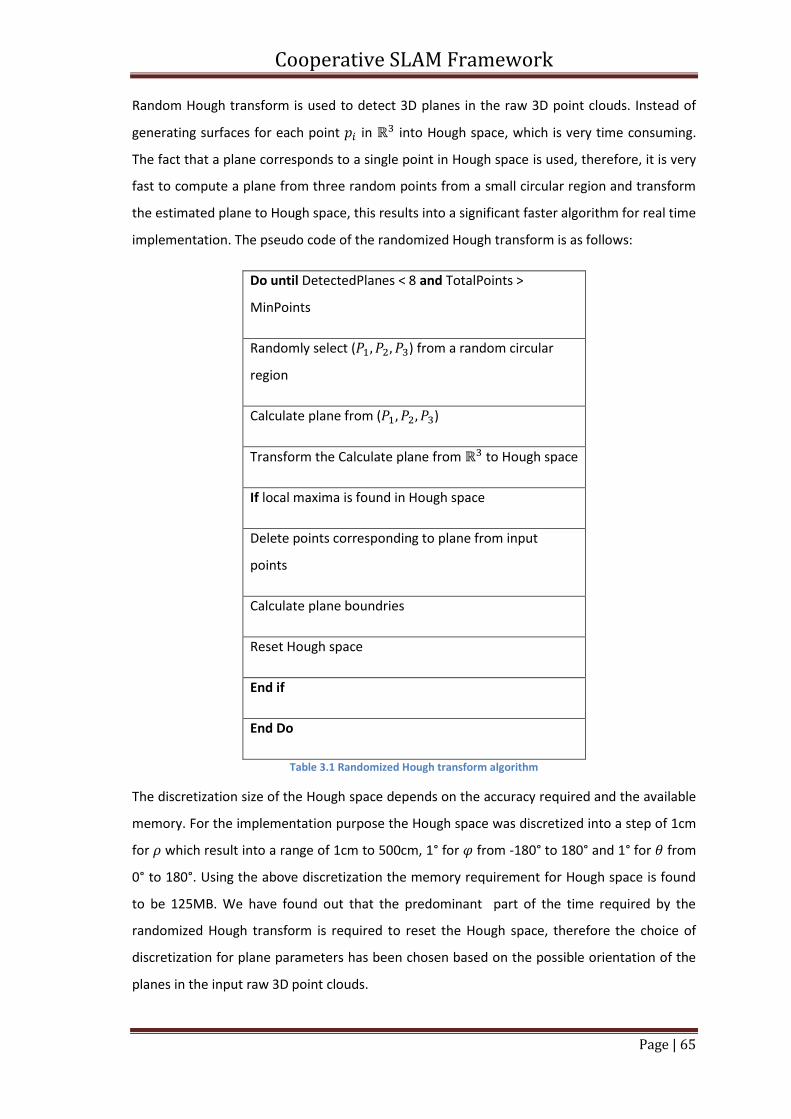
Cooperative SLAM Framework
Page | 65
Random Hough transform is used to detect 3D planes in the raw 3D point clouds. Instead of
generating surfaces for each point in into Hough space, which is very time consuming.
The fact that a plane corresponds to a single point in Hough space is used, therefore, it is very
fast to compute a plane from three random points from a small circular region and transform
the estimated plane to Hough space, this results into a significant faster algorithm for real time
implementation. The pseudo code of the randomized Hough transform is as follows:
Do until DetectedPlanes < 8 and TotalPoints >
MinPoints
Randomly select ( ) from a random circular
region
Calculate plane from ( )
Transform the Calculate plane from to Hough space
If local maxima is found in Hough space
Delete points corresponding to plane from input
points
Calculate plane boundries
Reset Hough space
End if
End Do
Table 3.1 Randomized Hough transform algorithm
The discretization size of the Hough space depends on the accuracy required and the available
memory. For the implementation purpose the Hough space was discretized into a step of 1cm
for which result into a range of 1cm to 500cm, 1° for from -180° to 180° and 1° for from
0° to 180°. Using the above discretization the memory requirement for Hough space is found
to be 125MB. We have found out that the predominant part of the time required by the
randomized Hough transform is required to reset the Hough space, therefore the choice of
discretization for plane parameters has been chosen based on the possible orientation of the
planes in the input raw 3D point clouds.
Cooperative SLAM Framework
Page | 66
3.3.3. Feature prediction from map
Feature prediction from the map or data association is an important and crucial step for the
correct working of the EKF based SLAM algorithm. Basically in this step the expected
measurements by the robot are generated. This step requires the sensor observation model.
TOM3D robot is equipped with the laser scanner to detect the line features from the
environment. The lines along with their parameters uncertainties are extracted as described in
section 3. The correction phase in fact calculates the amount of new information brought up
by the laser scanner measurements. The amount of new information or innovation brought up
by observing the already existing line feature is calculated as follows:
*
+ *
+ Eq. 3.32
Here is the expected observation which is calculated by using the sensor observation
model. The sensor observation model for the laser scanner system to extract the line feature is
defined by the following equation
( ) *
+ *
(
) ( )
+ Eq. 3.33
The sensor observation model takes as input the current robot pose ( ) and one
of the already mapped line features (
) described in global coordinate frame and
map it to the robot’s local coordinate frame (
)
. The covariance of the expected
feature observation is calculated as follows
, - [
] *
+ Eq. 3.34
Where is the Jacobian of the sensor observation model with respect to the robot pose and
is the Jacobian of the sensor observation model with respect to the feature.
0 ( ) ( )
1 Eq. 3.35
0 ( ) ( )
1 Eq. 3.36
The crucial issue here is the data association of the measured feature with the existing
feature in the map. There are many different strategies for data association [68]. Here two
strategies are being discussed namely Mahalanobis distance and K-D Tree.
Cooperative SLAM Framework
Page | 67
3.3.3.1 Mahalanobis Distance
Mahalanobis distance is a distance measure which is based on the correlation of two variables
and scale invariant. It basically measures the similarity of a measured data to a known data.
The Euclidean distance measure cannot be used here because of the two reasons. First, both
parameters of the line features are of different scales and, second, it doesn’t takes into
account the uncertainty of the parameters. The Mahalanobis distance criteria can be applied
iteratively on all the features of the existing map to find out which expected feature from the
existing map best matches to the measured feature. In other words we choose a feature with
minimum Mahalanobis distance (Maximum Likelihood) below some threshold. Mathematically
it is described as follows
Eq. 3.37
Here is the innovation and is the covariance of the innovation and is the squared
Mahalanobis distance for a constant probability density curve with locus cantered at
measured feature. The innovation covariance is found by adding the covariance of the
expected measurement and the measured feature covariance i.e.
Eq. 3.38
The covariance of the measured feature is found in section 3 is as follows
[
] Eq. 3.39
3.3.3.2 KD Tree
KD tree is a binary tree where K is the dimension of the data. It has storage requirements of
( ) where is the number of data point. It supports the nearest neighbor search scheme
which is important for estimated feature extraction from the map. The nodes within the KD
tree consist of two child pointers and a key. The number of item in the Key value represents
the D or dimension of the data. Let’s consider a concrete example in case of our SLAM
problem. After extracting number of line features from the range scan data the next step is to
extract the expected lines from the map at the given robot position. Here we assume that the
map consists of a set of lines or in other words a set of pair of values which define the
equation of line. Since we need two parameters and to define the line in Hessian normal
form therefore, we need a 2D-tree data structure to represent our feature based map. Each
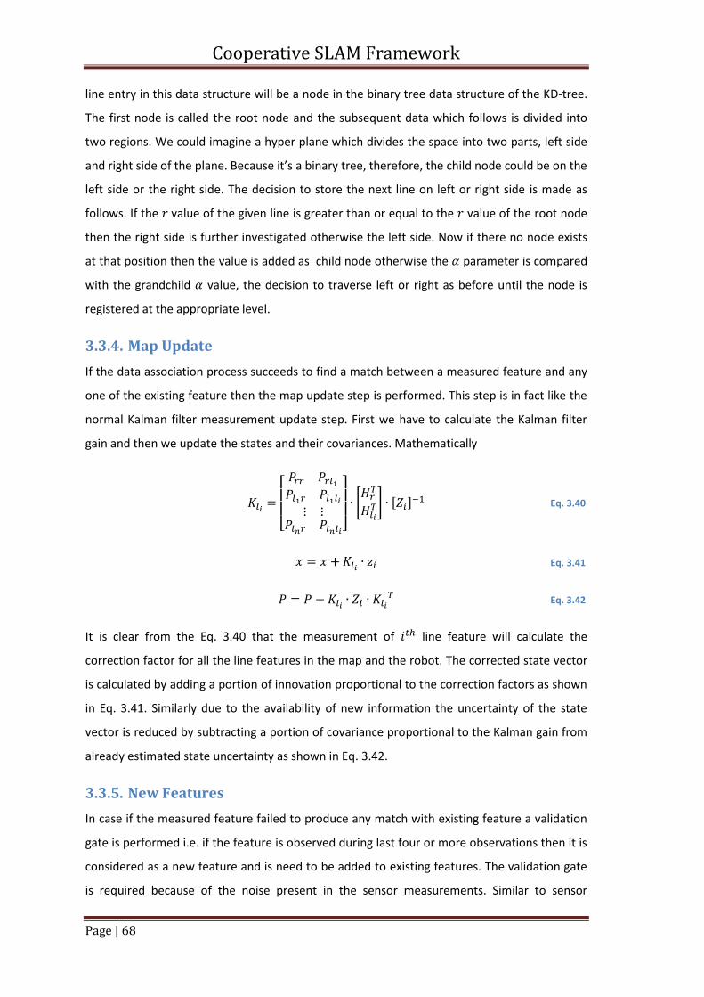
Cooperative SLAM Framework
Page | 68
line entry in this data structure will be a node in the binary tree data structure of the KD-tree.
The first node is called the root node and the subsequent data which follows is divided into
two regions. We could imagine a hyper plane which divides the space into two parts, left side
and right side of the plane. Because it’s a binary tree, therefore, the child node could be on the
left side or the right side. The decision to store the next line on left or right side is made as
follows. If the value of the given line is greater than or equal to the value of the root node
then the right side is further investigated otherwise the left side. Now if there no node exists
at that position then the value is added as child node otherwise the parameter is compared
with the grandchild value, the decision to traverse left or right as before until the node is
registered at the appropriate level.
3.3.4. Map Update
If the data association process succeeds to find a match between a measured feature and any
one of the existing feature then the map update step is performed. This step is in fact like the
normal Kalman filter measurement update step. First we have to calculate the Kalman filter
gain and then we update the states and their covariances. Mathematically
[
] *
+ , -
Eq. 3.40
Eq. 3.41
Eq. 3.42
It is clear from the Eq. 3.40 that the measurement of line feature will calculate the
correction factor for all the line features in the map and the robot. The corrected state vector
is calculated by adding a portion of innovation proportional to the correction factors as shown
in Eq. 3.41. Similarly due to the availability of new information the uncertainty of the state
vector is reduced by subtracting a portion of covariance proportional to the Kalman gain from
already estimated state uncertainty as shown in Eq. 3.42.
3.3.5. New Features
In case if the measured feature failed to produce any match with existing feature a validation
gate is performed i.e. if the feature is observed during last four or more observations then it is
considered as a new feature and is need to be added to existing features. The validation gate
is required because of the noise present in the sensor measurements. Similar to sensor
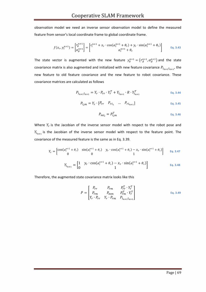
Cooperative SLAM Framework
Page | 69
observation model we need an inverse sensor observation model to define the measured
feature from sensor’s local coordinate frame to global coordinate frame.
( ) *
+ *
(
) ( )
+ Eq. 3.43
The state vector is augmented with the new feature (
) and the state
covariance matrix is also augmented and initialized with new feature covariance , the
new feature to old feature covariance and the new feature to robot covariance. These
covariance matrices are calculated as follows
Eq. 3.44
, - Eq. 3.45
Eq. 3.46
Where is the Jacobian of the inverse sensor model with respect to the robot pose and
is the Jacobian of the inverse sensor model with respect to the feature point. The
covariance of the measured feature is the same as in Eq. 3.39.
[ (
) ( ) (
) ( )
] Eq. 3.47
[ (
) ( )
] Eq. 3.48
Therefore, the augmented state covariance matrix looks like this
[
] Eq. 3.49
Cooperative SLAM Framework
Page | 70
3.4. Summary
This chapter describes in detail the core components of the SLAM algorithm for
implementation purposes. Active range sensors such as laser-scanner have advantage over the
passive sensors such as stereo camera systems because they are independent from
illumination and object reflection. Furthermore, they are accurate with long range
measurement where the stereo system have error variance which squares with the distance.
There are many other issues in the EKF based SLAM which are not discussed here but which
are important for the practical implementation of the EKF-SLAM algorithm, such as features’
signatures (color, length etc.), intelligent update of only relevant features.
The advantages of the EKF based SLAM algorithm lies in the simplicity of applying EKF
algorithm to the SLAM problem and it works well for small number of unique features. There
are few drawbacks of the EKF-SLAM algorithm. The computation requirements grow quadratic
ally to the number of features. It relies very heavily on the data association assumption,
therefore, errors in the data association results into divergence and ultimately explosion of the
filter. And the solution would not be optimal in case of non-Gaussian noise and strong non-
linearity in motion and observation models.
The topics which are important for the SLAM implementation are clustering, feature
extraction and data association. Various data clustering techniques which are useful and
applicable to range sensors are described. The techniques used for extraction of geometric
lines and planes are also described. Lines are extracted by using the non-linear least square
estimate technique. Where the planes are extracted by using Hough transformation process.
Then the features prediction step is explained which can use Mahalanobis distance based
technique for feature prediction or the KD-Tree based approach. And finally the map update
and augmentation process is described.
Cooperative SLAM Framework
Page | 71
Chapter 4. Cooperative SLAM (CSLAM)
For mobile robots to act autonomously in their environment there are two fundamentally
different approaches. One is the behavior based approach in which robots rely much on their
sensory to take decision. The second approach is the model based approach in which the
mobile robots model its surrounding environment. The model of the world around the mobile
robot is in the form of a map. In chapter 2.5 we have seen the different representations of the
maps which are useful to mobile robots. Mobile robots need the map to find their position in
the environment and plan their actions in the environment. SLAM answers the localization and
map building conundrum of the mobile robots in an unknown environment as both step
depend on each other. Various working SLAM flavors exist now days such as GMapping,
GridSLAM and DP-SLAM for research purpose. However no existing SLAM package is available
for multiple robots up to the knowledge of the author. This chapter formalizes the cooperative
SLAM strategy for multiple robots with different heterogeneous set of features.
4.1. SLAM for Heterogeneous features
The standard EKF based SLAM algorithm solution is for one type of features. In this section an
EKF based SLAM algorithm is described for a single robot and heterogeneous features. By
heterogeneous features means different kind of geometric features. One could extract and
model different kind of geometric features such as corners, lines, circles and planes from the
2D range scan data. Line features can easily be extracted from the 2D range scan
measurements of the laser range scanner such as SICK Laser scanner while the plane features
can easily be extracted from the 3D range measurements from the depth cameras such as
Kinect. Two parameters ( ) are required to fully describe a line as shown in Eq. 4.1 and
three parameters ( ) are required to fully describe a plane as shown in Eq. 4.2.
( ) ( ) Eq. 4.1
( ) ( ) ( ) ( ) ( ) Eq. 4.2
The parameters of a geometric feature can be augmented to the state vector as a new feature
on the discovery during the mobile robot moves in the environment. The set of features is
defined as map. The re-observation of the existing features is used to correct the pose of the
robot and helps to reduce the uncertainty of the robot pose and map. In the case of EKF based
SLAM algorithm the state vector and covariance matrix can be described as follows
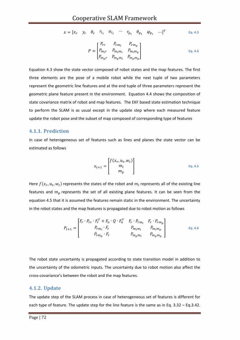
Cooperative SLAM Framework
Page | 72
, - Eq. 4.3
[
] Eq. 4.4
Equation 4.3 show the state vector composed of robot states and the map features. The first
three elements are the pose of a mobile robot while the next tuple of two parameters
represent the geometric line features and at the end tuple of three parameters represent the
geometric plane feature present in the environment. Equation 4.4 shows the composition of
state covariance matrix of robot and map features. The EKF based state estimation technique
to perform the SLAM is as usual except in the update step where each measured feature
update the robot pose and the subset of map composed of corresponding type of features
4.1.1. Prediction
In case of heterogeneous set of features such as lines and planes the state vector can be
estimated as follows
[
( )
] Eq. 4.5
Here ( ) represents the states of the robot and represents all of the existing line
features and represents the set of all existing plane features. It can be seen from the
equation 4.5 that it is assumed the features remain static in the environment. The uncertainty
in the robot states and the map features is propagated due to robot motion as follows
[
] Eq. 4.6
The robot state uncertainty is propagated according to state transition model in addition to
the uncertainty of the odometric inputs. The uncertainty due to robot motion also affect the
cross-covariance’s between the robot and the map features.
4.1.2. Update
The update step of the SLAM process in case of heterogeneous set of features is different for
each type of feature. The update step for the line feature is the same as in Eq. 3.32 – Eq.3.42.
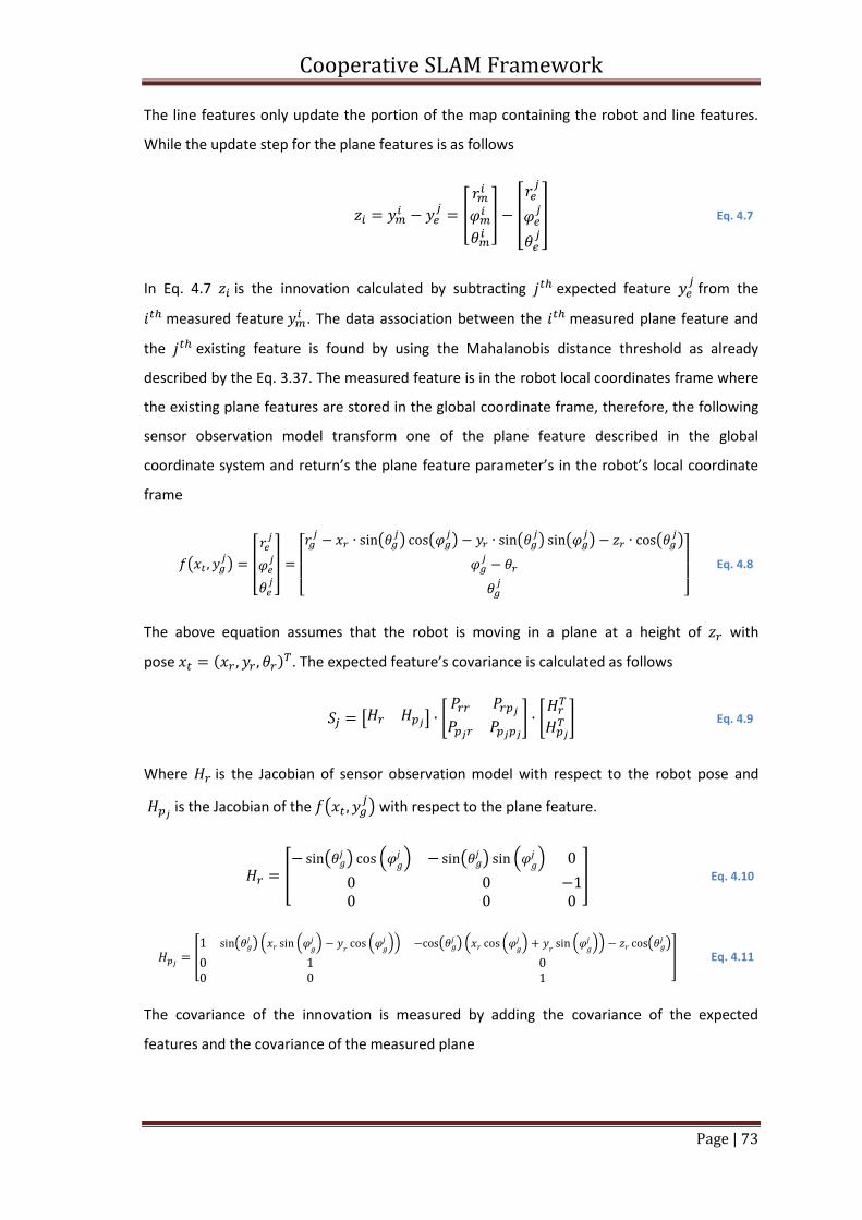
Cooperative SLAM Framework
Page | 73
The line features only update the portion of the map containing the robot and line features.
While the update step for the plane features is as follows
[
] [
] Eq. 4.7
In Eq. 4.7 is the innovation calculated by subtracting expected feature from the
measured feature . The data association between the measured plane feature and
the existing feature is found by using the Mahalanobis distance threshold as already
described by the Eq. 3.37. The measured feature is in the robot local coordinates frame where
the existing plane features are stored in the global coordinate frame, therefore, the following
sensor observation model transform one of the plane feature described in the global
coordinate system and return’s the plane feature parameter’s in the robot’s local coordinate
frame
( ) [
]
[ (
) (
) (
) (
) (
)
] Eq. 4.8
The above equation assumes that the robot is moving in a plane at a height of with
pose ( ) . The expected feature’s covariance is calculated as follows
[ ] *
+ *
+ Eq. 4.9
Where is the Jacobian of sensor observation model with respect to the robot pose and
is the Jacobian of the ( ) with respect to the plane feature.
[ (
) . / (
) . /
] Eq. 4.10
[ (
) . . /
.
// (
) . . /
.
// (
)
] Eq. 4.11
The covariance of the innovation is measured by adding the covariance of the expected
features and the covariance of the measured plane
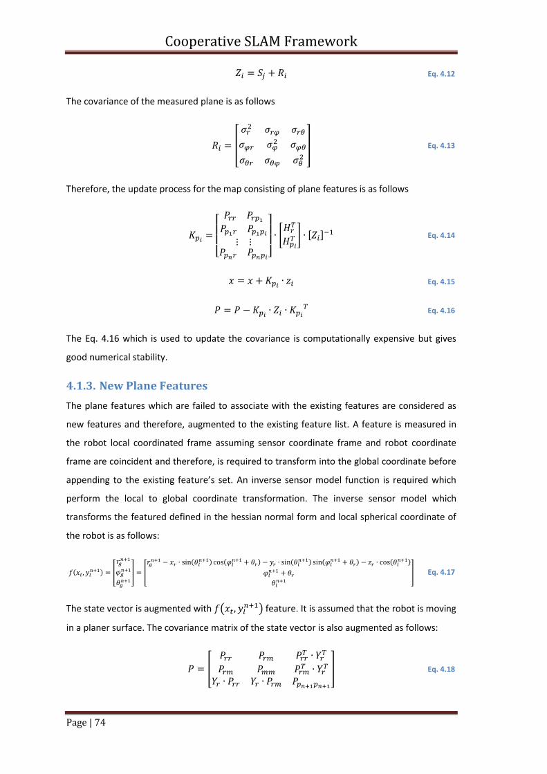
Cooperative SLAM Framework
Page | 74
Eq. 4.12
The covariance of the measured plane is as follows
[
] Eq. 4.13
Therefore, the update process for the map consisting of plane features is as follows
[
]
*
+ , -
Eq. 4.14
Eq. 4.15
Eq. 4.16
The Eq. 4.16 which is used to update the covariance is computationally expensive but gives
good numerical stability.
4.1.3. New Plane Features
The plane features which are failed to associate with the existing features are considered as
new features and therefore, augmented to the existing feature list. A feature is measured in
the robot local coordinated frame assuming sensor coordinate frame and robot coordinate
frame are coincident and therefore, is required to transform into the global coordinate before
appending to the existing feature’s set. An inverse sensor model function is required which
perform the local to global coordinate transformation. The inverse sensor model which
transforms the featured defined in the hessian normal form and local spherical coordinate of
the robot is as follows:
( ) [
] [
(
) ( ) (
) ( ) (
)
] Eq. 4.17
The state vector is augmented with ( ) feature. It is assumed that the robot is moving
in a planer surface. The covariance matrix of the state vector is also augmented as follows:
[
] Eq. 4.18
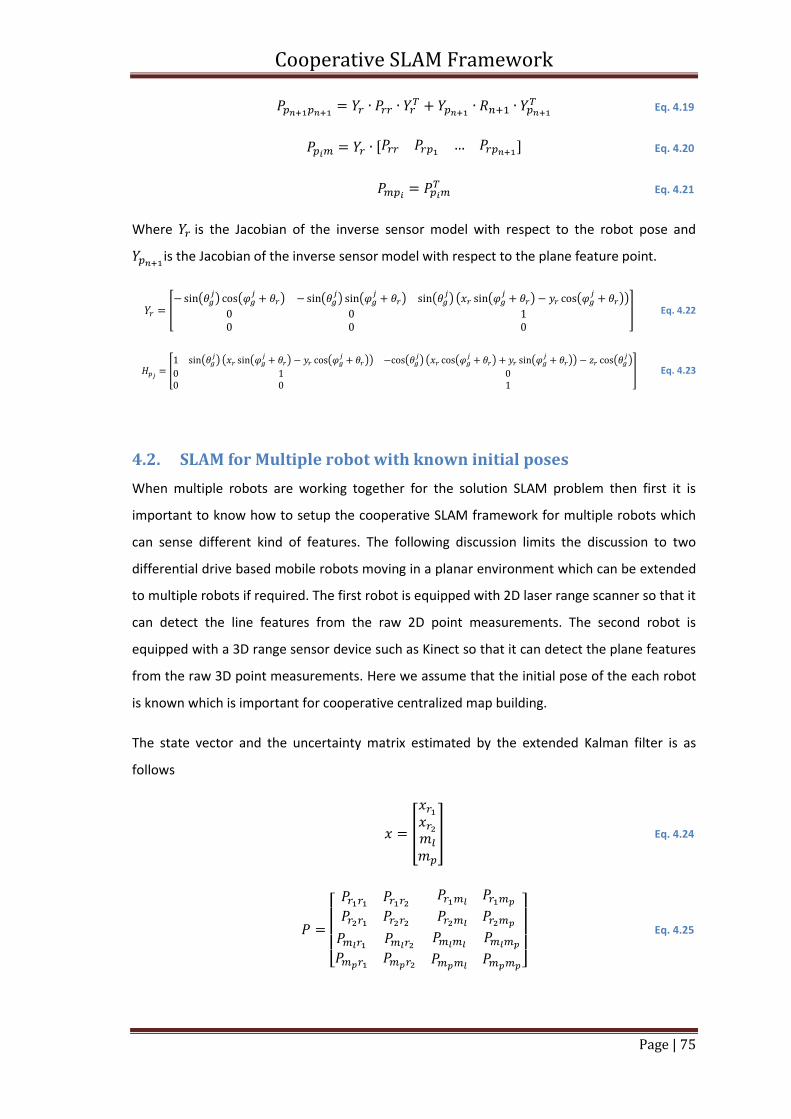
Cooperative SLAM Framework
Page | 75
Eq. 4.19
, - Eq. 4.20
Eq. 4.21
Where is the Jacobian of the inverse sensor model with respect to the robot pose and
is the Jacobian of the inverse sensor model with respect to the plane feature point.
[ (
) (
) (
) (
) (
) ( (
) (
))
] Eq. 4.22
[ (
) ( ( ) (
)) (
) ( ( ) (
)) (
)
] Eq. 4.23
4.2. SLAM for Multiple robot with known initial poses
When multiple robots are working together for the solution SLAM problem then first it is
important to know how to setup the cooperative SLAM framework for multiple robots which
can sense different kind of features. The following discussion limits the discussion to two
differential drive based mobile robots moving in a planar environment which can be extended
to multiple robots if required. The first robot is equipped with 2D laser range scanner so that it
can detect the line features from the raw 2D point measurements. The second robot is
equipped with a 3D range sensor device such as Kinect so that it can detect the plane features
from the raw 3D point measurements. Here we assume that the initial pose of the each robot
is known which is important for cooperative centralized map building.
The state vector and the uncertainty matrix estimated by the extended Kalman filter is as
follows
[
] Eq. 4.24
[
]
Eq. 4.25
Cooperative SLAM Framework
Page | 76
Here ( ) is the state vector for the first robot and ( )
is the
state vector for the second robot. ( ) is the subset of the total map which
consist of only line features extracted from the 2D range sensor and ( ) is the
subset of consists of plane features extracted from the 3D range sensor.
4.3. Summary
In this chapter a mathematical cooperative SLAM framework is formalized which is based on
the extended Kalman filter. First an EKF based SLAM formulation is developed for the 2D
geometric lines and 3D geometric planes. Each of the major implementation steps for the
SLAM; prediction, update and the augmentation is described.
Later the formulation considers multiple robots in the formulization. The state vector is
composed of individual robot state vector, 2D line features and the 3D plane features. The
formulization assumes the initial relative robot pose are known.
Cooperative SLAM Framework
Page | 77
Chapter 5.
Framework and Hardware Development
A mobile robot system usually consist of hardware components such as sensors, actuators and
control unit for low level tasks related to mobile robots. These sensors, actuators and control
algorithms are controlled by a firmware running in the control unit. Usually this control unit
communicates with the high level algorithms running on a desktop computer for their tasks
management or tele-control. Carrying out the task by a mobile robot requires the integration
of several modules.
Therefore, a scalable cooperative multi-robot system is developed to address the current
challenge of controlling, configuring and management of multiple ground and aerial robots
with heterogeneous capabilities. The operation of the system for cooperative map building
scenario is shown in Figure 5.1. Mobile agents can be created or configured dynamically at
run-time in the existing team of mobile robots to perform tasks. Creation means assigning a
unique ID, adding set of sensors and their poses via a graphical user interface for a physical
mobile robot which is to be added into a team of mobile robots. Furthermore, to provide
format for communication protocols of commands and reports between the mobile robot and
computer control interface. Therefore, when sensor data is received from a mobile robot, it is
parsed according to the robot’s report protocol format and then stored in to a database. The
mobile robots sensors data in the database is categorized according to the sensor type. The
structured logging of sensor data according to sensor type into the database enables mapping
and localization modules to quickly process the relevant information.
A mapping module which is a part of ground coordinator generates the online map and
updates it automatically from the database. It makes the global map by using all range type
sensors registered in the database from all mobile robots in the network. Based on the robot’s
ID, range sensor’s data and pose from the database an online mesh is generated and rendered
into the global map. 3D object models of robots along with their current pose are also
rendered in to the map.
Another aspect of the system is the modular firmware architecture and a universal hardware
board for ground mobile robots. The firmware architecture consists of multiple modules which
can be enabled, disables or configured on the fly. Modules are defined as behaviors, sensors
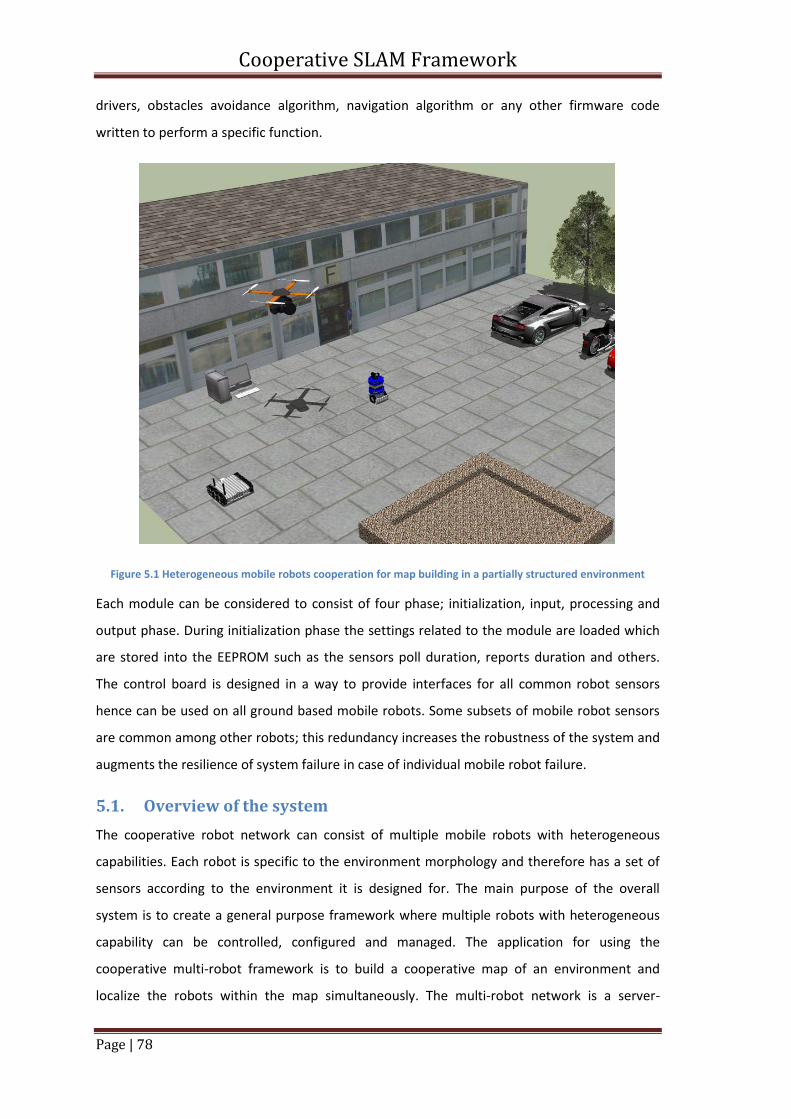
Cooperative SLAM Framework
Page | 78
drivers, obstacles avoidance algorithm, navigation algorithm or any other firmware code
written to perform a specific function.
Figure 5.1 Heterogeneous mobile robots cooperation for map building in a partially structured environment
Each module can be considered to consist of four phase; initialization, input, processing and
output phase. During initialization phase the settings related to the module are loaded which
are stored into the EEPROM such as the sensors poll duration, reports duration and others.
The control board is designed in a way to provide interfaces for all common robot sensors
hence can be used on all ground based mobile robots. Some subsets of mobile robot sensors
are common among other robots; this redundancy increases the robustness of the system and
augments the resilience of system failure in case of individual mobile robot failure.
5.1. Overview of the system
The cooperative robot network can consist of multiple mobile robots with heterogeneous
capabilities. Each robot is specific to the environment morphology and therefore has a set of
sensors according to the environment it is designed for. The main purpose of the overall
system is to create a general purpose framework where multiple robots with heterogeneous
capability can be controlled, configured and managed. The application for using the
cooperative multi-robot framework is to build a cooperative map of an environment and
localize the robots within the map simultaneously. The multi-robot network is a server-
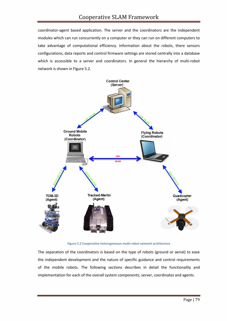
Cooperative SLAM Framework
Page | 79
coordinator-agent based application. The server and the coordinators are the independent
modules which can run concurrently on a computer or they can run on different computers to
take advantage of computational efficiency. Information about the robots, there sensors
configurations, data reports and control firmware settings are stored centrally into a database
which is accessible to a server and coordinators. In general the hierarchy of multi-robot
network is shown in Figure 5.2.
Figure 5.2 Cooperative heterogeneous multi-robot network architecture
The separation of the coordinators is based on the type of robots (ground or aerial) to ease
the independent development and the nature of specific guidance and control requirements
of the mobile robots. The following sections describes in detail the functionality and
implementation for each of the overall system components; server, coordinates and agents.
LAN WLAN
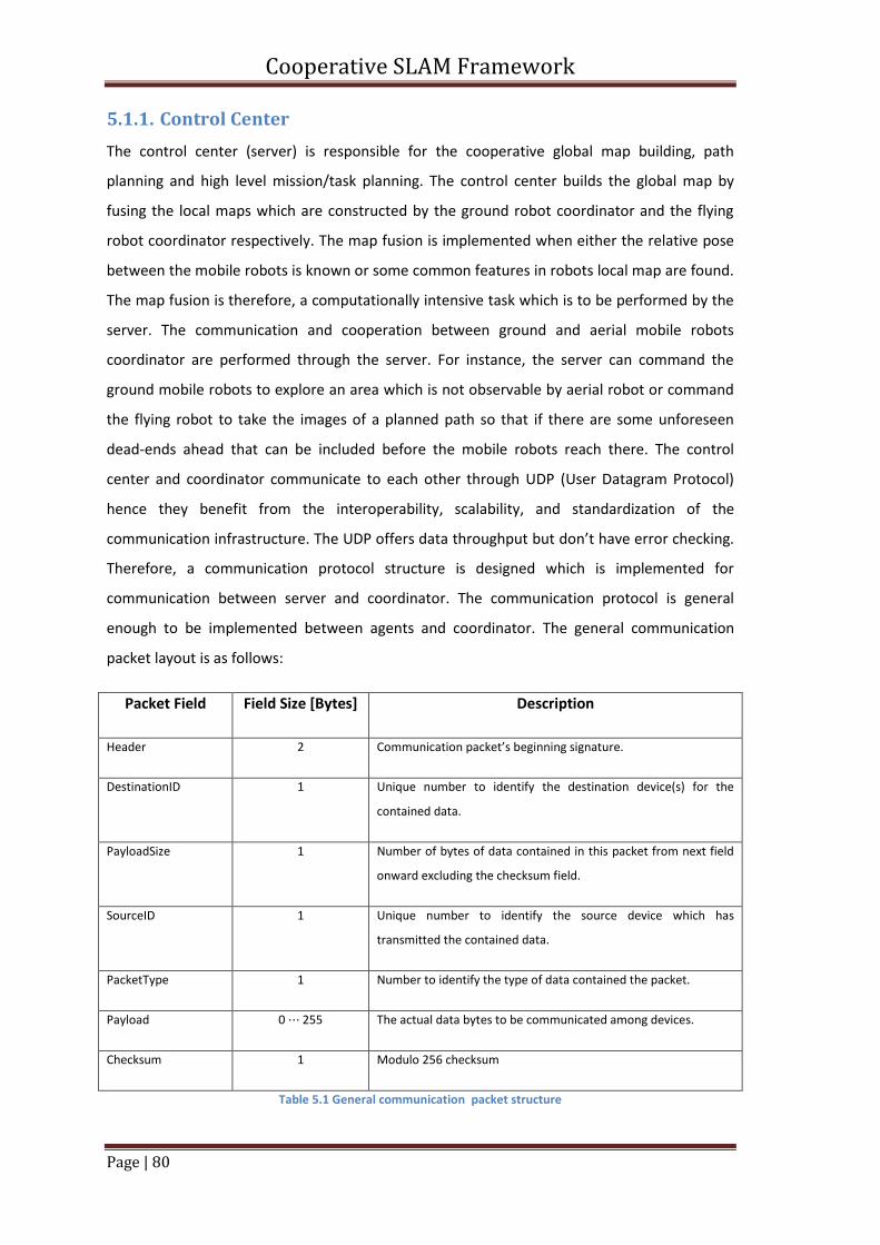
Cooperative SLAM Framework
Page | 80
5.1.1. Control Center
The control center (server) is responsible for the cooperative global map building, path
planning and high level mission/task planning. The control center builds the global map by
fusing the local maps which are constructed by the ground robot coordinator and the flying
robot coordinator respectively. The map fusion is implemented when either the relative pose
between the mobile robots is known or some common features in robots local map are found.
The map fusion is therefore, a computationally intensive task which is to be performed by the
server. The communication and cooperation between ground and aerial mobile robots
coordinator are performed through the server. For instance, the server can command the
ground mobile robots to explore an area which is not observable by aerial robot or command
the flying robot to take the images of a planned path so that if there are some unforeseen
dead-ends ahead that can be included before the mobile robots reach there. The control
center and coordinator communicate to each other through UDP (User Datagram Protocol)
hence they benefit from the interoperability, scalability, and standardization of the
communication infrastructure. The UDP offers data throughput but don’t have error checking.
Therefore, a communication protocol structure is designed which is implemented for
communication between server and coordinator. The communication protocol is general
enough to be implemented between agents and coordinator. The general communication
packet layout is as follows:
Packet Field Field Size [Bytes] Description
Header 2 Communication packet’s beginning signature.
DestinationID 1 Unique number to identify the destination device(s) for the
contained data.
PayloadSize 1 Number of bytes of data contained in this packet from next field
onward excluding the checksum field.
SourceID 1 Unique number to identify the source device which has
transmitted the contained data.
PacketType 1 Number to identify the type of data contained the packet.
Payload 0 255 The actual data bytes to be communicated among devices.
Checksum 1 Modulo 256 checksum
Table 5.1 General communication packet structure
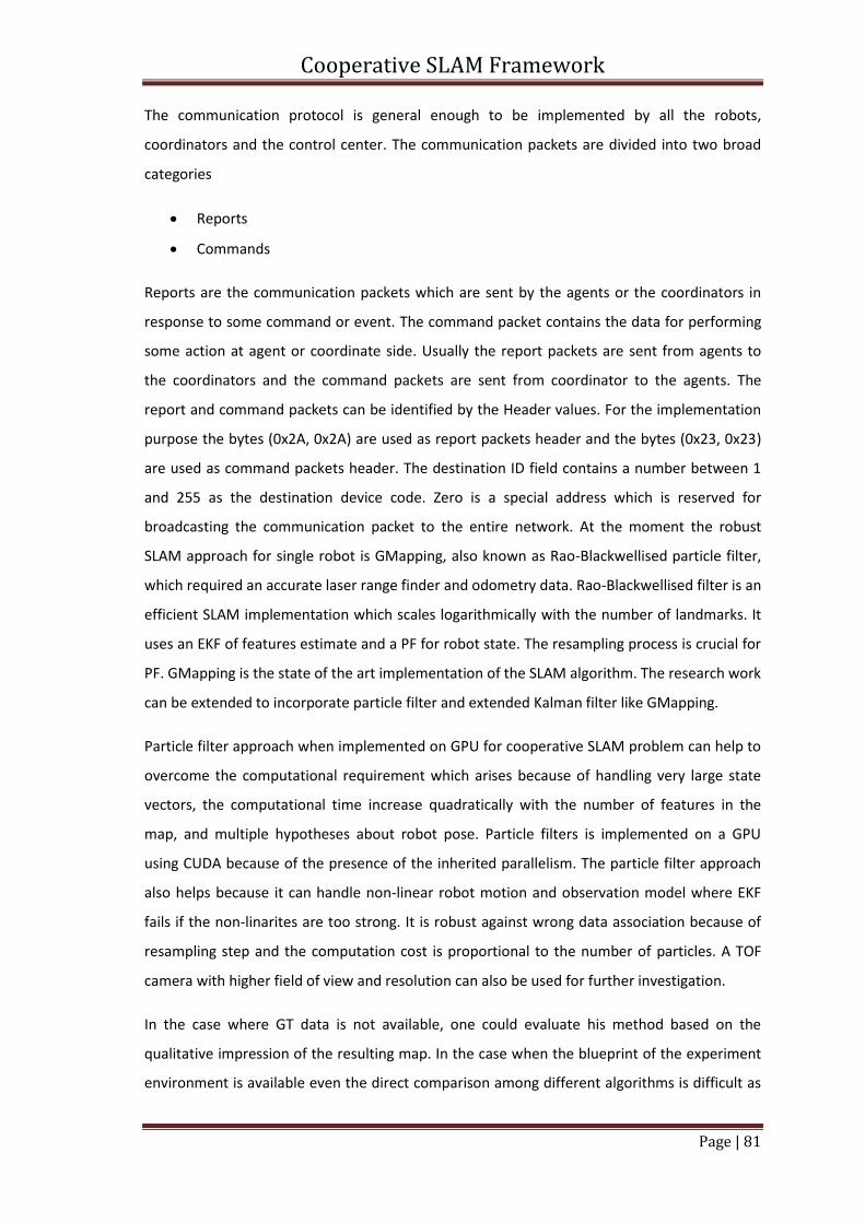
Cooperative SLAM Framework
Page | 81
The communication protocol is general enough to be implemented by all the robots,
coordinators and the control center. The communication packets are divided into two broad
categories
Reports
Commands
Reports are the communication packets which are sent by the agents or the coordinators in
response to some command or event. The command packet contains the data for performing
some action at agent or coordinate side. Usually the report packets are sent from agents to
the coordinators and the command packets are sent from coordinator to the agents. The
report and command packets can be identified by the Header values. For the implementation
purpose the bytes (0x2A, 0x2A) are used as report packets header and the bytes (0x23, 0x23)
are used as command packets header. The destination ID field contains a number between 1
and 255 as the destination device code. Zero is a special address which is reserved for
broadcasting the communication packet to the entire network. At the moment the robust
SLAM approach for single robot is GMapping, also known as Rao-Blackwellised particle filter,
which required an accurate laser range finder and odometry data. Rao-Blackwellised filter is an
efficient SLAM implementation which scales logarithmically with the number of landmarks. It
uses an EKF of features estimate and a PF for robot state. The resampling process is crucial for
PF. GMapping is the state of the art implementation of the SLAM algorithm. The research work
can be extended to incorporate particle filter and extended Kalman filter like GMapping.
Particle filter approach when implemented on GPU for cooperative SLAM problem can help to
overcome the computational requirement which arises because of handling very large state
vectors, the computational time increase quadratically with the number of features in the
map, and multiple hypotheses about robot pose. Particle filters is implemented on a GPU
using CUDA because of the presence of the inherited parallelism. The particle filter approach
also helps because it can handle non-linear robot motion and observation model where EKF
fails if the non-linarites are too strong. It is robust against wrong data association because of
resampling step and the computation cost is proportional to the number of particles. A TOF
camera with higher field of view and resolution can also be used for further investigation.
In the case where GT data is not available, one could evaluate his method based on the
qualitative impression of the resulting map. In the case when the blueprint of the experiment
environment is available even the direct comparison among different algorithms is difficult as
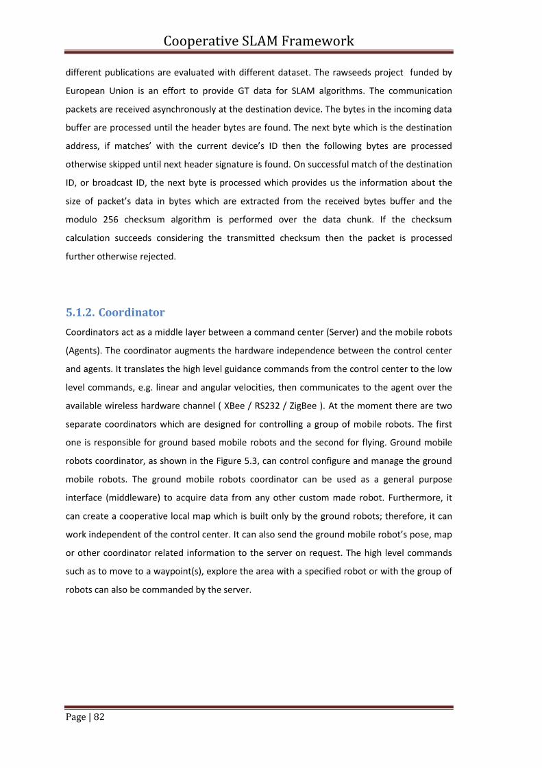
Cooperative SLAM Framework
Page | 82
different publications are evaluated with different dataset. The rawseeds project funded by
European Union is an effort to provide GT data for SLAM algorithms. The communication
packets are received asynchronously at the destination device. The bytes in the incoming data
buffer are processed until the header bytes are found. The next byte which is the destination
address, if matches’ with the current device’s ID then the following bytes are processed
otherwise skipped until next header signature is found. On successful match of the destination
ID, or broadcast ID, the next byte is processed which provides us the information about the
size of packet’s data in bytes which are extracted from the received bytes buffer and the
modulo 256 checksum algorithm is performed over the data chunk. If the checksum
calculation succeeds considering the transmitted checksum then the packet is processed
further otherwise rejected.
5.1.2. Coordinator
Coordinators act as a middle layer between a command center (Server) and the mobile robots
(Agents). The coordinator augments the hardware independence between the control center
and agents. It translates the high level guidance commands from the control center to the low
level commands, e.g. linear and angular velocities, then communicates to the agent over the
available wireless hardware channel ( XBee / RS232 / ZigBee ). At the moment there are two
separate coordinators which are designed for controlling a group of mobile robots. The first
one is responsible for ground based mobile robots and the second for flying. Ground mobile
robots coordinator, as shown in the Figure 5.3, can control configure and manage the ground
mobile robots. The ground mobile robots coordinator can be used as a general purpose
interface (middleware) to acquire data from any other custom made robot. Furthermore, it
can create a cooperative local map which is built only by the ground robots; therefore, it can
work independent of the control center. It can also send the ground mobile robot’s pose, map
or other coordinator related information to the server on request. The high level commands
such as to move to a waypoint(s), explore the area with a specified robot or with the group of
robots can also be commanded by the server.
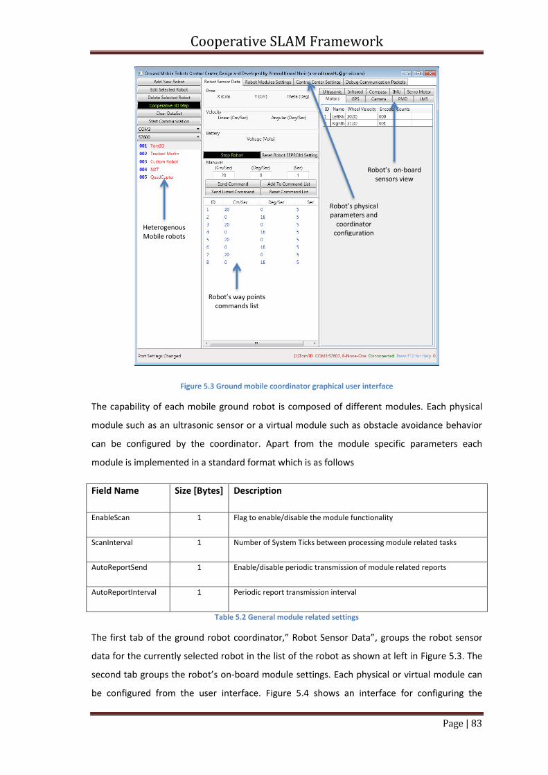
Cooperative SLAM Framework
Page | 83
Figure 5.3 Ground mobile coordinator graphical user interface
The capability of each mobile ground robot is composed of different modules. Each physical
module such as an ultrasonic sensor or a virtual module such as obstacle avoidance behavior
can be configured by the coordinator. Apart from the module specific parameters each
module is implemented in a standard format which is as follows
Field Name Size [Bytes] Description
EnableScan 1 Flag to enable/disable the module functionality
ScanInterval 1 Number of System Ticks between processing module related tasks
AutoReportSend 1 Enable/disable periodic transmission of module related reports
AutoReportInterval 1 Periodic report transmission interval
Table 5.2 General module related settings
The first tab of the ground robot coordinator,” Robot Sensor Data”, groups the robot sensor
data for the currently selected robot in the list of the robot as shown at left in Figure 5.3. The
second tab groups the robot’s on-board module settings. Each physical or virtual module can
be configured from the user interface. Figure 5.4 shows an interface for configuring the
Robot’s on-board sensors view
Robot’s physical parameters and
coordinator configuration
Robot’s way points commands list
Heterogenous Mobile robots
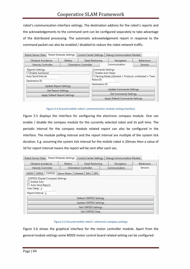
Cooperative SLAM Framework
Page | 84
robot’s communication interface settings. The destination address for the robot’s reports and
the acknowledgements to the command sent can be configured separately to take advantage
of the distributed processing. The automatic acknowledgement report in response to the
command packet can also be enabled / disabled to reduce the robot network traffic.
Figure 5.4 Ground mobile robot's communication module setting interface
Figure 5.5 displays the interface for configuring the electronic compass module. One can
enable / disable the compass module for the currently selected robot and its poll time. The
periodic interval for the compass module related report can also be configured in the
interface. The module polling interval and the report interval are multiple of the system tick
duration. E.g. assuming the system tick interval for the mobile robot is 20msec then a value of
50 for report interval means the report will be sent after each sec.
Figure 5.5 Ground mobile robot's electronic compass settings
Figure 5.6 shows the graphical interface for the motor controller module. Apart from the
general module settings some MD03 motor control board related setting can be configured.
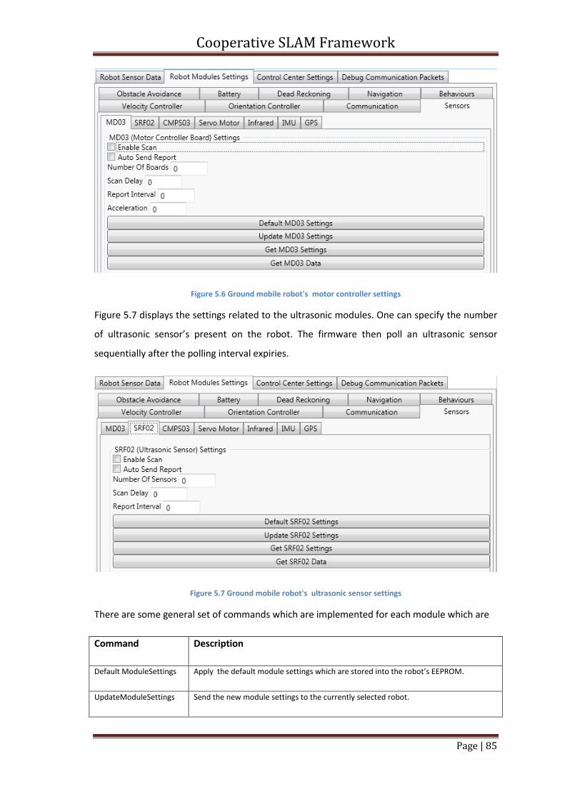
Cooperative SLAM Framework
Page | 85
Figure 5.6 Ground mobile robot's motor controller settings
Figure 5.7 displays the settings related to the ultrasonic modules. One can specify the number
of ultrasonic sensor’s present on the robot. The firmware then poll an ultrasonic sensor
sequentially after the polling interval expiries.
Figure 5.7 Ground mobile robot's ultrasonic sensor settings
There are some general set of commands which are implemented for each module which are
Command Description
Default ModuleSettings Apply the default module settings which are stored into the robot’s EEPROM.
UpdateModuleSettings Send the new module settings to the currently selected robot.
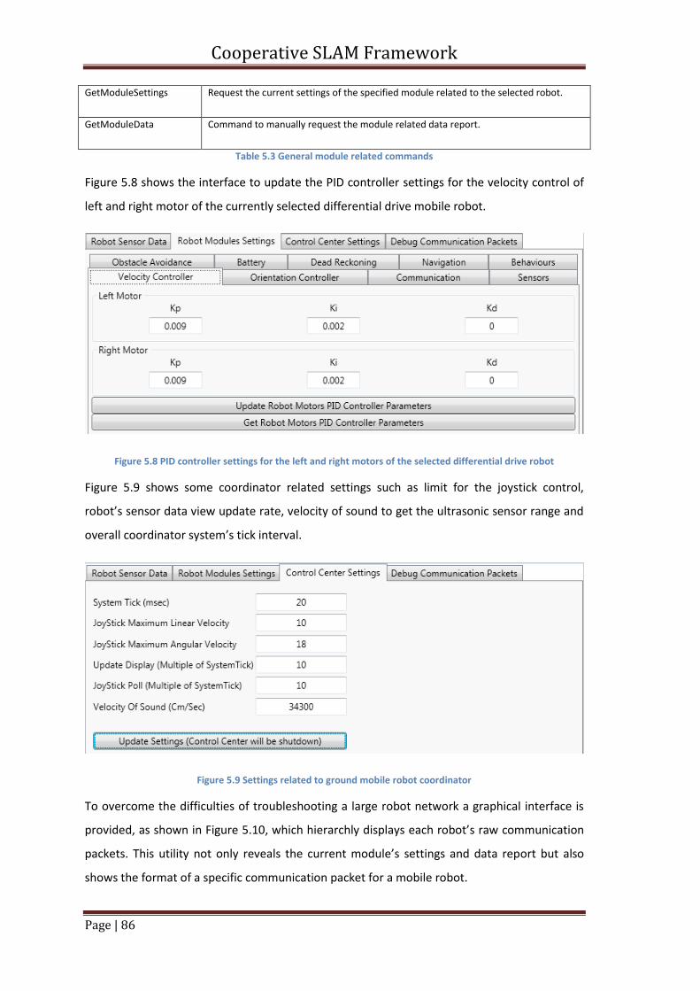
Cooperative SLAM Framework
Page | 86
GetModuleSettings Request the current settings of the specified module related to the selected robot.
GetModuleData Command to manually request the module related data report.
Table 5.3 General module related commands
Figure 5.8 shows the interface to update the PID controller settings for the velocity control of
left and right motor of the currently selected differential drive mobile robot.
Figure 5.8 PID controller settings for the left and right motors of the selected differential drive robot
Figure 5.9 shows some coordinator related settings such as limit for the joystick control,
robot’s sensor data view update rate, velocity of sound to get the ultrasonic sensor range and
overall coordinator system’s tick interval.
Figure 5.9 Settings related to ground mobile robot coordinator
To overcome the difficulties of troubleshooting a large robot network a graphical interface is
provided, as shown in Figure 5.10, which hierarchly displays each robot’s raw communication
packets. This utility not only reveals the current module’s settings and data report but also
shows the format of a specific communication packet for a mobile robot.
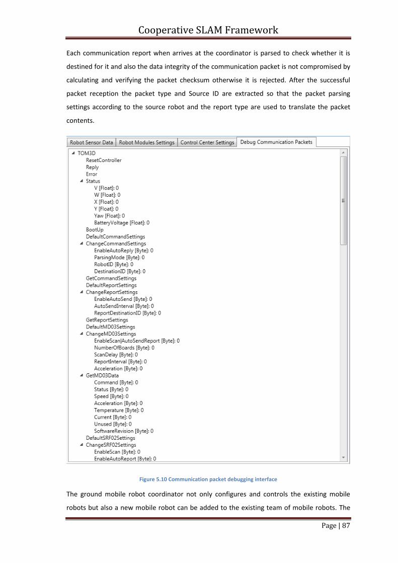
Cooperative SLAM Framework
Page | 87
Each communication report when arrives at the coordinator is parsed to check whether it is
destined for it and also the data integrity of the communication packet is not compromised by
calculating and verifying the packet checksum otherwise it is rejected. After the successful
packet reception the packet type and Source ID are extracted so that the packet parsing
settings according to the source robot and the report type are used to translate the packet
contents.
Figure 5.10 Communication packet debugging interface
The ground mobile robot coordinator not only configures and controls the existing mobile
robots but also a new mobile robot can be added to the existing team of mobile robots. The
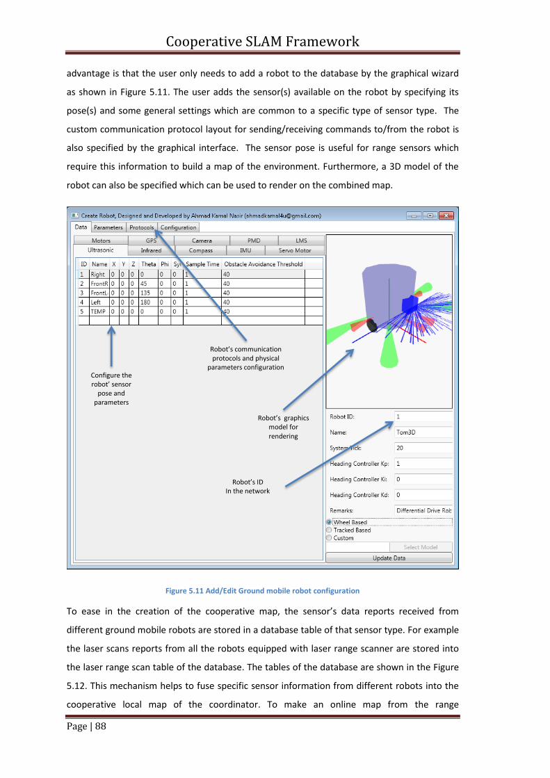
Cooperative SLAM Framework
Page | 88
advantage is that the user only needs to add a robot to the database by the graphical wizard
as shown in Figure 5.11. The user adds the sensor(s) available on the robot by specifying its
pose(s) and some general settings which are common to a specific type of sensor type. The
custom communication protocol layout for sending/receiving commands to/from the robot is
also specified by the graphical interface. The sensor pose is useful for range sensors which
require this information to build a map of the environment. Furthermore, a 3D model of the
robot can also be specified which can be used to render on the combined map.
Figure 5.11 Add/Edit Ground mobile robot configuration
To ease in the creation of the cooperative map, the sensor’s data reports received from
different ground mobile robots are stored in a database table of that sensor type. For example
the laser scans reports from all the robots equipped with laser range scanner are stored into
the laser range scan table of the database. The tables of the database are shown in the Figure
5.12. This mechanism helps to fuse specific sensor information from different robots into the
cooperative local map of the coordinator. To make an online map from the range
Robot’s graphics model for rendering
Robot’s communication protocols and physical
parameters configuration
Robot’s ID In the network
Configure the robot’ sensor
pose and parameters
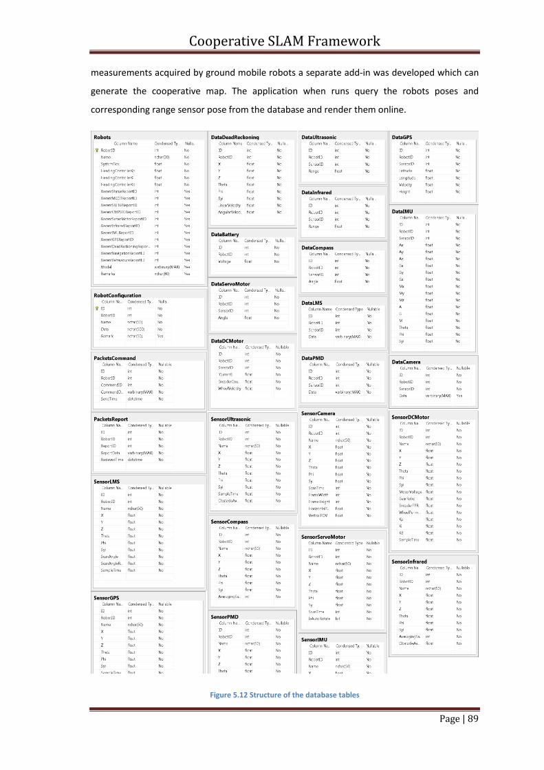
Cooperative SLAM Framework
Page | 89
measurements acquired by ground mobile robots a separate add-in was developed which can
generate the cooperative map. The application when runs query the robots poses and
corresponding range sensor pose from the database and render them online.
Figure 5.12 Structure of the database tables
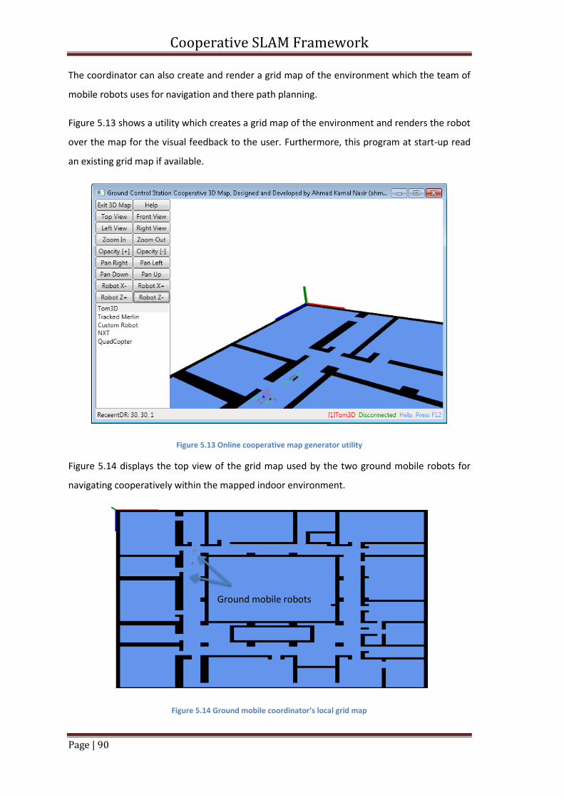
Cooperative SLAM Framework
Page | 90
The coordinator can also create and render a grid map of the environment which the team of
mobile robots uses for navigation and there path planning.
Figure 5.13 shows a utility which creates a grid map of the environment and renders the robot
over the map for the visual feedback to the user. Furthermore, this program at start-up read
an existing grid map if available.
Figure 5.13 Online cooperative map generator utility
Figure 5.14 displays the top view of the grid map used by the two ground mobile robots for
navigating cooperatively within the mapped indoor environment.
Figure 5.14 Ground mobile coordinator’s local grid map
Ground mobile robots
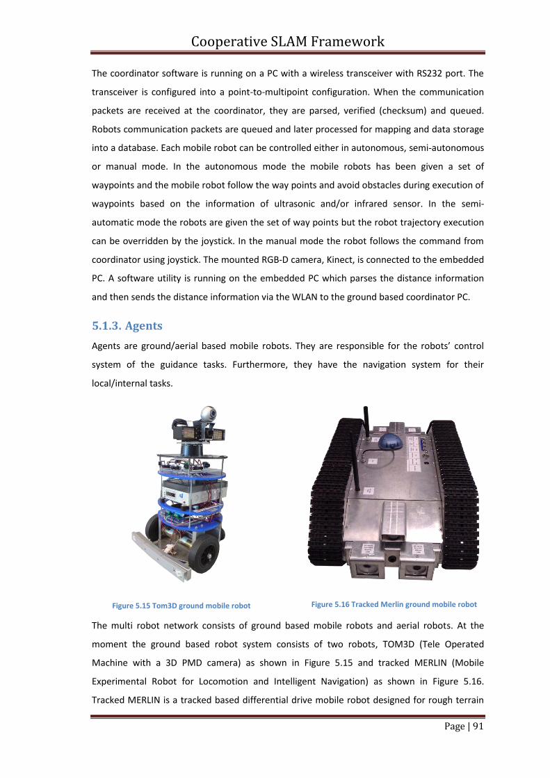
Cooperative SLAM Framework
Page | 91
The coordinator software is running on a PC with a wireless transceiver with RS232 port. The
transceiver is configured into a point-to-multipoint configuration. When the communication
packets are received at the coordinator, they are parsed, verified (checksum) and queued.
Robots communication packets are queued and later processed for mapping and data storage
into a database. Each mobile robot can be controlled either in autonomous, semi-autonomous
or manual mode. In the autonomous mode the mobile robots has been given a set of
waypoints and the mobile robot follow the way points and avoid obstacles during execution of
waypoints based on the information of ultrasonic and/or infrared sensor. In the semi-
automatic mode the robots are given the set of way points but the robot trajectory execution
can be overridden by the joystick. In the manual mode the robot follows the command from
coordinator using joystick. The mounted RGB-D camera, Kinect, is connected to the embedded
PC. A software utility is running on the embedded PC which parses the distance information
and then sends the distance information via the WLAN to the ground based coordinator PC.
5.1.3. Agents
Agents are ground/aerial based mobile robots. They are responsible for the robots’ control
system of the guidance tasks. Furthermore, they have the navigation system for their
local/internal tasks.
Figure 5.15 Tom3D ground mobile robot
Figure 5.16 Tracked Merlin ground mobile robot
The multi robot network consists of ground based mobile robots and aerial robots. At the
moment the ground based robot system consists of two robots, TOM3D (Tele Operated
Machine with a 3D PMD camera) as shown in Figure 5.15 and tracked MERLIN (Mobile
Experimental Robot for Locomotion and Intelligent Navigation) as shown in Figure 5.16.
Tracked MERLIN is a tracked based differential drive mobile robot designed for rough terrain
Cooperative SLAM Framework
Page | 92
in an outdoor environment. TOM3D is a ground based mobile robot which is designed for
indoor environment. Each robot is equipped with a different set of sensors e.g. TOM3D is
equipped with gyroscope, accelerometer, digital compass, magnetometer, ultrasonic sensor,
infrared sensor, bumper switches, a Kinect camera and a laser scanner.
For data processing of Kinect camera and laser scanner an embedded PC is mounted on
TOM3D which runs a 1.8 GHz Pentium M processor and equipped with 1GB RAM. The wheels
of TOM3D are integrated with high resolution quadrature encoders. The ground based tracked
MERLIN mobile robot is equipped with digital compass, GPS, ultrasonic sensors and track drive
motors integrated with quadrature encoders. Furthermore, it has front and rear wireless
cameras and microphones. Both ground based robots are equipped with 2.4GHz, 802.15.4
based 500mW RF transceivers which can be configured in a point-to-multipoint mode. The
camera images from the TOM3D robot are transmitted by the built-in WiFi of the embedded
PC. Where the camera images from the Tracked MERLIN robot are transmitted by a 5.8GHz
transmitter which can be multiplexed to transmit the front or rear camera by the control
board.
5.2. Firmware and Hardware
The control board and the firmware are also designed to be modular so that they can be used
and customized by any robot requirement. The firmware is developed with in such a way that
a variety of sensor’s drivers such as sonar, compass, IR, etc. are developed which can be
enabled or disabled for a particular robot configuration.
5.2.1. Firmware
Each ground based mobile robot’s control board is running a control system firmware. The
firmware is designed in a modular way so that each robot’s firmware can be reconfigured
wirelessly to enable or disable a particular sensor and its configuration parameters for control
and reports according to the availability of that sensor for that robot. Therefore the scalability
was kept in mind while developing the firmware. Each module has some common general
settings and communication packets which are described in Table 5.2 and Table 5.3. This
format for the modules and communication packets was developed by keeping in mind that
the future expansions to the existing features are easier to be implemented.
Since each robot has a different set of modules, therefore, for the ease of implementation of
the firmware for different robots, all the module settings for a specific robot are grouped
together in a configuration file. To develop a firmware for a robot the user can use DaVE [104]
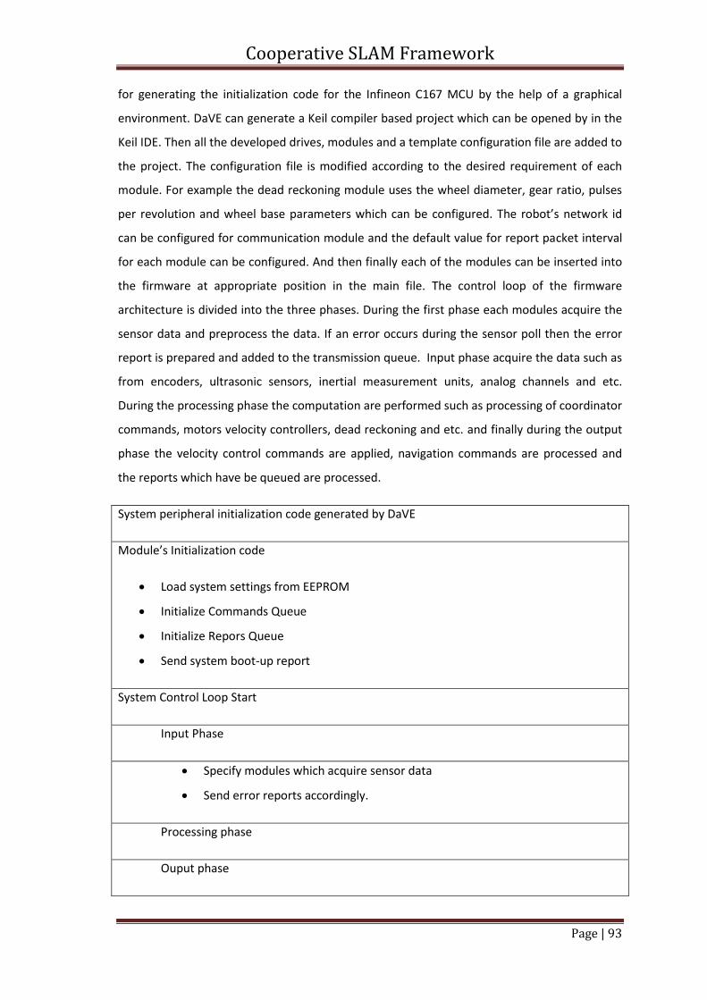
Cooperative SLAM Framework
Page | 93
for generating the initialization code for the Infineon C167 MCU by the help of a graphical
environment. DaVE can generate a Keil compiler based project which can be opened by in the
Keil IDE. Then all the developed drives, modules and a template configuration file are added to
the project. The configuration file is modified according to the desired requirement of each
module. For example the dead reckoning module uses the wheel diameter, gear ratio, pulses
per revolution and wheel base parameters which can be configured. The robot’s network id
can be configured for communication module and the default value for report packet interval
for each module can be configured. And then finally each of the modules can be inserted into
the firmware at appropriate position in the main file. The control loop of the firmware
architecture is divided into the three phases. During the first phase each modules acquire the
sensor data and preprocess the data. If an error occurs during the sensor poll then the error
report is prepared and added to the transmission queue. Input phase acquire the data such as
from encoders, ultrasonic sensors, inertial measurement units, analog channels and etc.
During the processing phase the computation are performed such as processing of coordinator
commands, motors velocity controllers, dead reckoning and etc. and finally during the output
phase the velocity control commands are applied, navigation commands are processed and
the reports which have be queued are processed.
System peripheral initialization code generated by DaVE
Module’s Initialization code
Load system settings from EEPROM
Initialize Commands Queue
Initialize Repors Queue
Send system boot-up report
System Control Loop Start
Input Phase
Specify modules which acquire sensor data
Send error reports accordingly.
Processing phase
Ouput phase
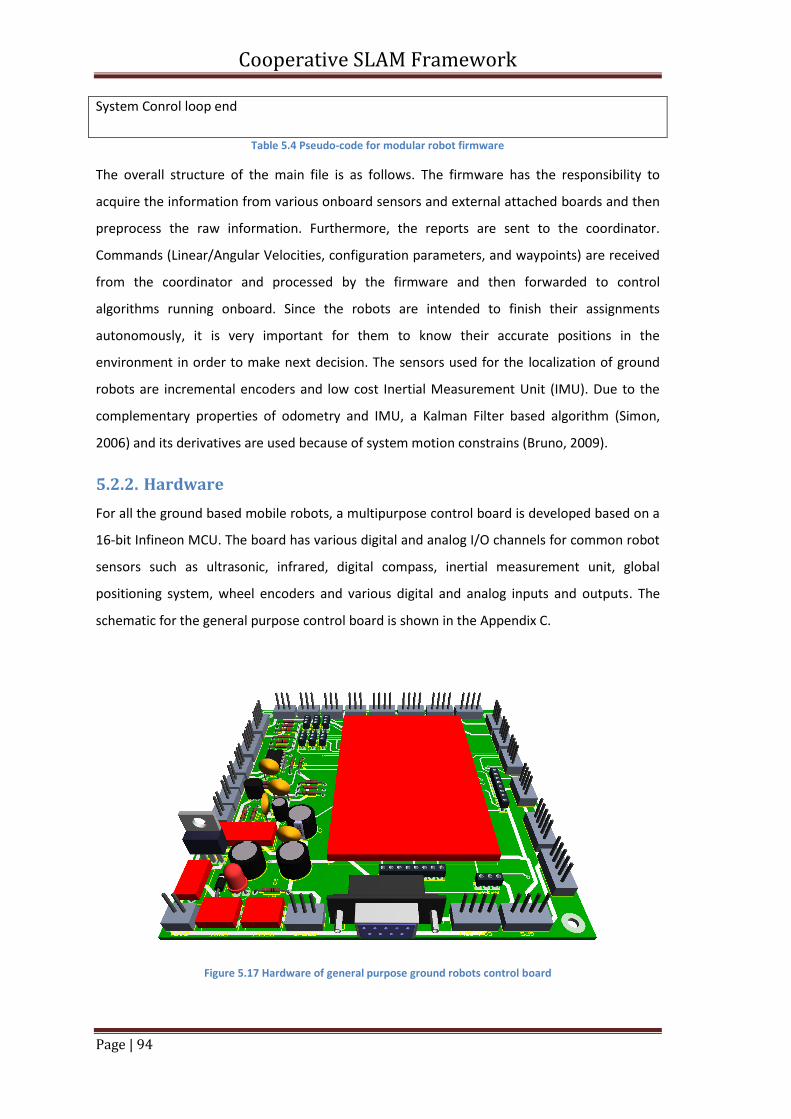
Cooperative SLAM Framework
Page | 94
System Conrol loop end
Table 5.4 Pseudo-code for modular robot firmware
The overall structure of the main file is as follows. The firmware has the responsibility to
acquire the information from various onboard sensors and external attached boards and then
preprocess the raw information. Furthermore, the reports are sent to the coordinator.
Commands (Linear/Angular Velocities, configuration parameters, and waypoints) are received
from the coordinator and processed by the firmware and then forwarded to control
algorithms running onboard. Since the robots are intended to finish their assignments
autonomously, it is very important for them to know their accurate positions in the
environment in order to make next decision. The sensors used for the localization of ground
robots are incremental encoders and low cost Inertial Measurement Unit (IMU). Due to the
complementary properties of odometry and IMU, a Kalman Filter based algorithm (Simon,
2006) and its derivatives are used because of system motion constrains (Bruno, 2009).
5.2.2. Hardware
For all the ground based mobile robots, a multipurpose control board is developed based on a
16-bit Infineon MCU. The board has various digital and analog I/O channels for common robot
sensors such as ultrasonic, infrared, digital compass, inertial measurement unit, global
positioning system, wheel encoders and various digital and analog inputs and outputs. The
schematic for the general purpose control board is shown in the Appendix C.
Figure 5.17 Hardware of general purpose ground robots control board
Cooperative SLAM Framework
Page | 95
For the communication of the control board with the coordinator it is also equipped with a
radio frequency modem as shown in . The radio frequency modem communicates with the
control board via serial port and uses the IEEE 802.15.4 standard to communicate with the
remote node. The communication modems are configured in a point to multi-point
configuration. The master modem which is attached to the coordinator PC can receive the
reports from all the slave modems mounted on the ground agents. Where the command
transmitted by the master is received by all the slaves and the slave which is the destination of
communication packet process it further where all the other reject and wait for another
packet.
Figure 5.18 Agents Communication Modem based on IEEE 802.15.4
The communication packet uses module 256 checksum algorithms for transmission error
checking. The wireless transceiver has the built-in error checking capability but this added
error checksum mechanism ensures that the designed protocol remains independent from the
hardware medium of transmission.
5.3. Simulation Environment
To overcome the difficulties of the hardware implementation, resources limitation and to
reduce the algorithms development time a mobile robot simulation environment can be used.
There are many commercial and open source mobile robot simulation softwares available in
the market. Any mobile robot simulation software such as PSG, Webbots, USARSim or others
can be used to simulate the robot’s sensor data. The presented research work proposes
USARSim. USARSim [46] is a simulation environment used in the presented research work
which is based on the Unreal Tournament game engine. The simulation environment as shown
in the Figure 5.19 provides us virtual ground and aerial robots in a map. The ground robot
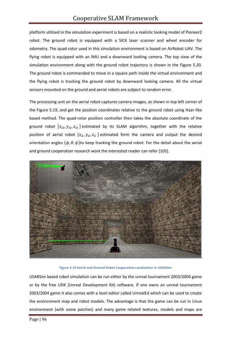
Cooperative SLAM Framework
Page | 96
platform utilized in the simulation experiment is based on a realistic looking model of Pioneer2
robot. The ground robot is equipped with a SICK laser scanner and wheel encoder for
odometry. The quad-rotor used in this simulation environment is based on AirRobot UAV. The
flying robot is equipped with an IMU and a downward looking camera. The top view of the
simulation environment along with the ground robot trajectory is shown in the Figure 5.20.
The ground robot is commanded to move in a square path inside the virtual environment and
the flying robot is tracking the ground robot by downward looking camera. All the virtual
sensors mounted on the ground and aerial robots are subject to random error.
The processing unit on the aerial robot captures camera images, as shown in top left corner of
the Figure 5.19, and get the position coordinates relative to the ground robot using Haar-like
based method. The quad-rotor position controller then takes the absolute coordinate of the
ground robot , - estimated by its SLAM algorithm, together with the relative
position of aerial robot , - estimated form the camera and output the desired
orientation angles ( )to keep tracking the ground robot. For the detail about the aerial
and ground cooperation research work the interested reader can refer [105].
Figure 5.19 Aerial and Ground Robot Cooperative Localization In USARSim
USARSim based robot simulation can be run either by the unreal tournament 2003/2004 game
or by the free UDK (Unreal Development Kit) software. If one owns an unreal tournament
2003/2004 game it also comes with a level editor called UnrealEd which can be used to create
the environment map and robot models. The advantage is that the game can be run in Linux
environment (with some patches) and many game related textures, models and maps are
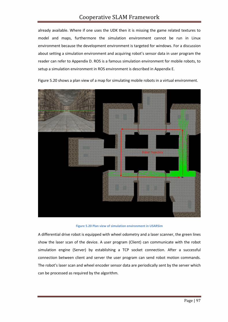
Cooperative SLAM Framework
Page | 97
already available. Where if one uses the UDK then it is missing the game related textures to
model and maps, furthermore the simulation environment cannot be run in Linux
environment because the development environment is targeted for windows. For a discussion
about setting a simulation environment and acquiring robot’s sensor data in user program the
reader can refer to Appendix D. ROS is a famous simulation environment for mobile robots, to
setup a simulation environment in ROS environment is described in Appendix E.
Figure 5.20 shows a plan view of a map for simulating mobile robots in a virtual environment.
Figure 5.20 Plan view of simulation environment in USARSim
A differential drive robot is equipped with wheel odometry and a laser scanner, the green lines
show the laser scan of the device. A user program (Client) can communicate with the robot
simulation engine (Server) by establishing a TCP socket connection. After a successful
connection between client and server the user program can send robot motion commands.
The robot’s laser scan and wheel encoder sensor data are periodically sent by the server which
can be processed as required by the algorithm.
Cooperative SLAM Framework
Page | 98
5.4. Summary
In this chapter the architecture of a multi-robot system is described, which consists of
heterogeneous capabilities aerial and ground mobile robots for making online map
cooperatively. The overall system consist of three parts; Control center, Coordinators and the
Agents.
First the overall system architecture is described then other features such as communication
protocol and ground Coordinator software interfaces are discussed for ground mobile robots.
Afterwards, the hardware and firmware of ground and aerial mobile robots were introduced.
And finally for rapid development of a multi-robot system a simulation environment based on
USARSim is introduced. USARSim is a high-fidelity simulation environment for mobile robots
based on the Unreal Tournament game engine. It is being interfaced to the proposed system
so that it can acquire sensors data from multiple simulated robots with heterogeneous
capabilities to generate the online map cooperatively
The overall system is designed in such a way that the future scalability of the robot network
and the system features can be assured. The ground based mobile robot coordinator can be
used as a general purpose robot control interface to acquire mobile robot’s sensor data, so as
to control the mobile robot using the joystick and remotely configure robot’s firmware
features using the graphic user interface on a windows based PC. Another novel feature of the
ground mobile robots coordinator is the online generation and rendering of the meshes
created from the mobile robots range data cloud points for online creation of the map.
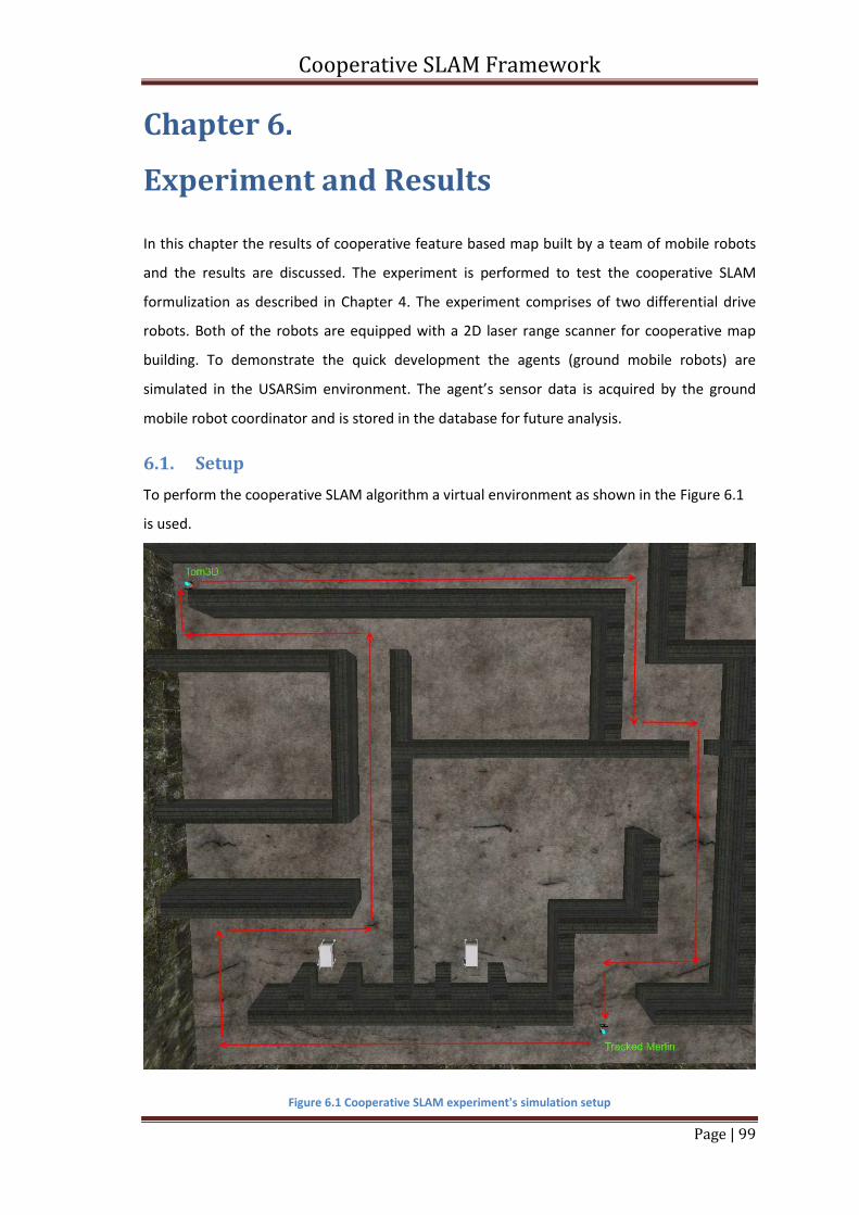
Cooperative SLAM Framework
Page | 99
Chapter 6.
Experiment and Results
In this chapter the results of cooperative feature based map built by a team of mobile robots
and the results are discussed. The experiment is performed to test the cooperative SLAM
formulization as described in Chapter 4. The experiment comprises of two differential drive
robots. Both of the robots are equipped with a 2D laser range scanner for cooperative map
building. To demonstrate the quick development the agents (ground mobile robots) are
simulated in the USARSim environment. The agent’s sensor data is acquired by the ground
mobile robot coordinator and is stored in the database for future analysis.
6.1. Setup
To perform the cooperative SLAM algorithm a virtual environment as shown in the Figure 6.1
is used.
Figure 6.1 Cooperative SLAM experiment's simulation setup
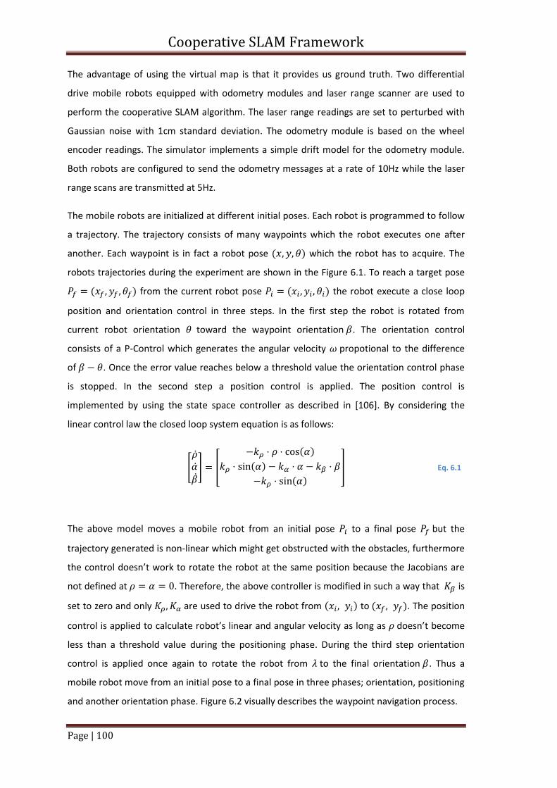
Cooperative SLAM Framework
Page | 100
The advantage of using the virtual map is that it provides us ground truth. Two differential
drive mobile robots equipped with odometry modules and laser range scanner are used to
perform the cooperative SLAM algorithm. The laser range readings are set to perturbed with
Gaussian noise with 1cm standard deviation. The odometry module is based on the wheel
encoder readings. The simulator implements a simple drift model for the odometry module.
Both robots are configured to send the odometry messages at a rate of 10Hz while the laser
range scans are transmitted at 5Hz.
The mobile robots are initialized at different initial poses. Each robot is programmed to follow
a trajectory. The trajectory consists of many waypoints which the robot executes one after
another. Each waypoint is in fact a robot pose ( ) which the robot has to acquire. The
robots trajectories during the experiment are shown in the Figure 6.1. To reach a target pose
( ) from the current robot pose ( ) the robot execute a close loop
position and orientation control in three steps. In the first step the robot is rotated from
current robot orientation toward the waypoint orientation . The orientation control
consists of a P-Control which generates the angular velocity propotional to the difference
of . Once the error value reaches below a threshold value the orientation control phase
is stopped. In the second step a position control is applied. The position control is
implemented by using the state space controller as described in [106]. By considering the
linear control law the closed loop system equation is as follows:
[
] [
( )
( )
( )
] Eq. 6.1
The above model moves a mobile robot from an initial pose to a final pose but the
trajectory generated is non-linear which might get obstructed with the obstacles, furthermore
the control doesn’t work to rotate the robot at the same position because the Jacobians are
not defined at . Therefore, the above controller is modified in such a way that is
set to zero and only are used to drive the robot from ( ) to ( ). The position
control is applied to calculate robot’s linear and angular velocity as long as doesn’t become
less than a threshold value during the positioning phase. During the third step orientation
control is applied once again to rotate the robot from to the final orientation . Thus a
mobile robot move from an initial pose to a final pose in three phases; orientation, positioning
and another orientation phase. Figure 6.2 visually describes the waypoint navigation process.
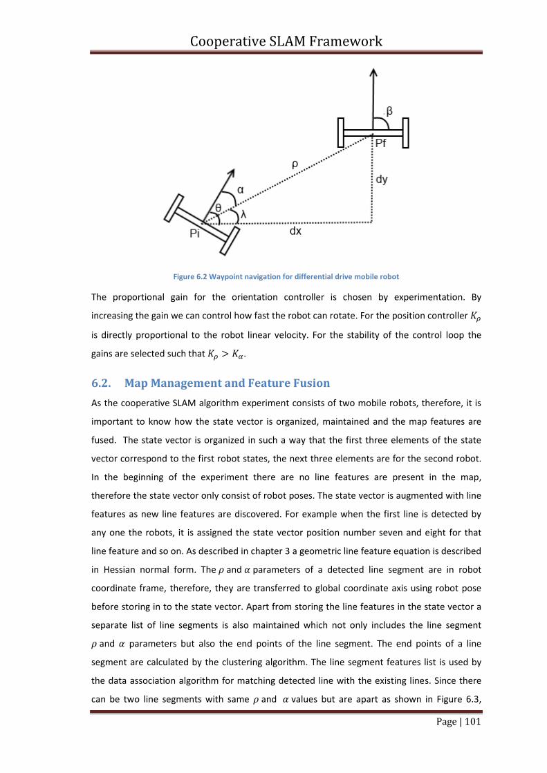
Cooperative SLAM Framework
Page | 101
Figure 6.2 Waypoint navigation for differential drive mobile robot
The proportional gain for the orientation controller is chosen by experimentation. By
increasing the gain we can control how fast the robot can rotate. For the position controller
is directly proportional to the robot linear velocity. For the stability of the control loop the
gains are selected such that .
6.2. Map Management and Feature Fusion
As the cooperative SLAM algorithm experiment consists of two mobile robots, therefore, it is
important to know how the state vector is organized, maintained and the map features are
fused. The state vector is organized in such a way that the first three elements of the state
vector correspond to the first robot states, the next three elements are for the second robot.
In the beginning of the experiment there are no line features are present in the map,
therefore the state vector only consist of robot poses. The state vector is augmented with line
features as new line features are discovered. For example when the first line is detected by
any one the robots, it is assigned the state vector position number seven and eight for that
line feature and so on. As described in chapter 3 a geometric line feature equation is described
in Hessian normal form. The and parameters of a detected line segment are in robot
coordinate frame, therefore, they are transferred to global coordinate axis using robot pose
before storing in to the state vector. Apart from storing the line features in the state vector a
separate list of line segments is also maintained which not only includes the line segment
and parameters but also the end points of the line segment. The end points of a line
segment are calculated by the clustering algorithm. The line segment features list is used by
the data association algorithm for matching detected line with the existing lines. Since there
can be two line segments with same and values but are apart as shown in Figure 6.3,
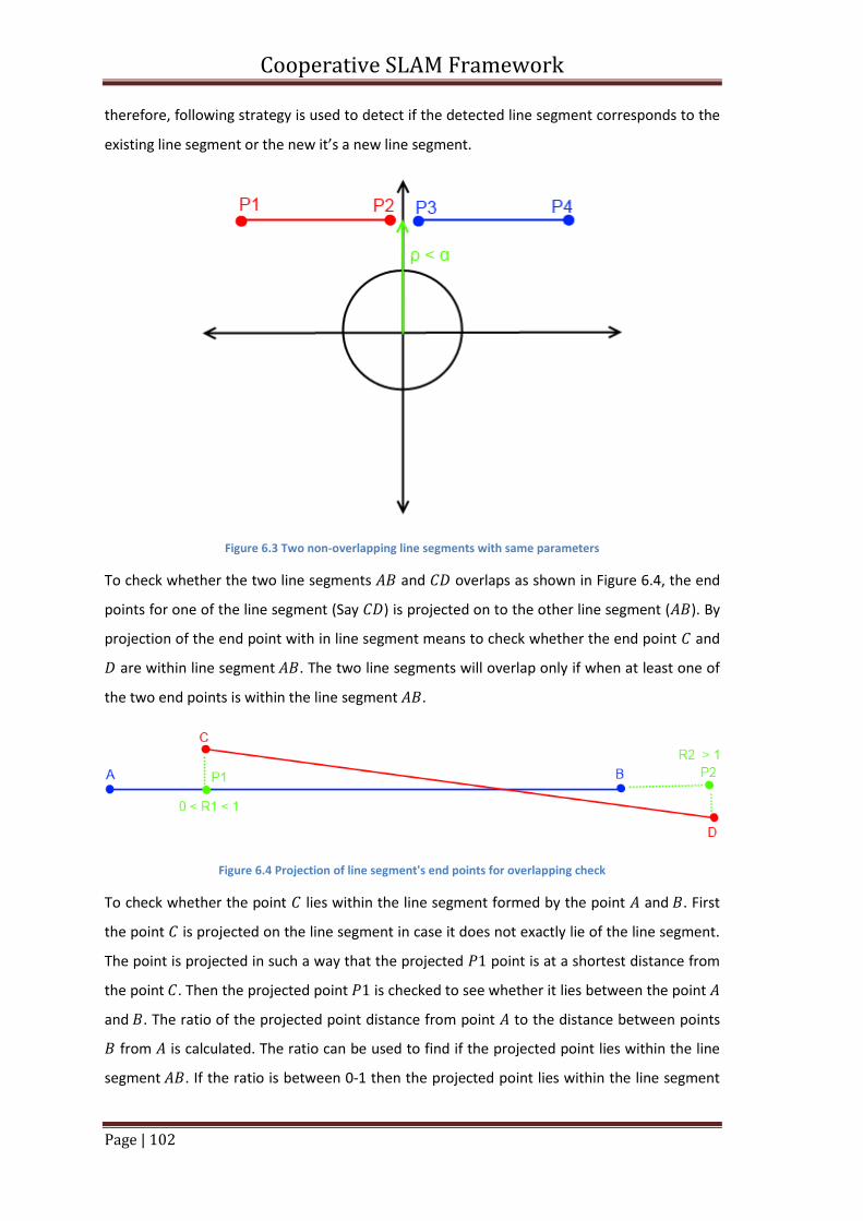
Cooperative SLAM Framework
Page | 102
therefore, following strategy is used to detect if the detected line segment corresponds to the
existing line segment or the new it’s a new line segment.
Figure 6.3 Two non-overlapping line segments with same parameters
To check whether the two line segments and overlaps as shown in Figure 6.4, the end
points for one of the line segment (Say ) is projected on to the other line segment ( ). By
projection of the end point with in line segment means to check whether the end point and
are within line segment . The two line segments will overlap only if when at least one of
the two end points is within the line segment .
Figure 6.4 Projection of line segment's end points for overlapping check
To check whether the point lies within the line segment formed by the point and . First
the point is projected on the line segment in case it does not exactly lie of the line segment.
The point is projected in such a way that the projected point is at a shortest distance from
the point . Then the projected point is checked to see whether it lies between the point
and . The ratio of the projected point distance from point to the distance between points
from is calculated. The ratio can be used to find if the projected point lies within the line
segment . If the ratio is between 0-1 then the projected point lies within the line segment
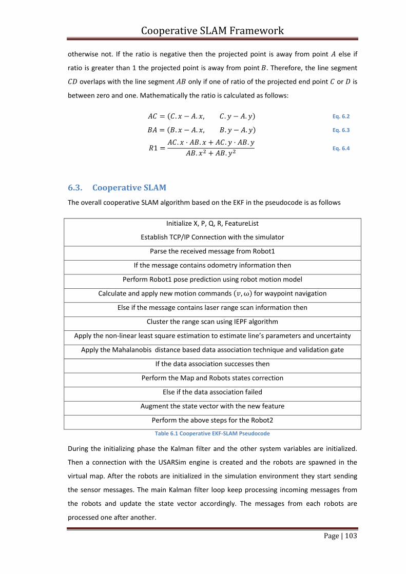
Cooperative SLAM Framework
Page | 103
otherwise not. If the ratio is negative then the projected point is away from point else if
ratio is greater than 1 the projected point is away from point . Therefore, the line segment
overlaps with the line segment only if one of ratio of the projected end point or is
between zero and one. Mathematically the ratio is calculated as follows:
( ) Eq. 6.2
( ) Eq. 6.3
Eq. 6.4
6.3. Cooperative SLAM
The overall cooperative SLAM algorithm based on the EKF in the pseudocode is as follows
Initialize X, P, Q, R, FeatureList
Establish TCP/IP Connection with the simulator
Parse the received message from Robot1
If the message contains odometry information then
Perform Robot1 pose prediction using robot motion model
Calculate and apply new motion commands ( ) for waypoint navigation
Else if the message contains laser range scan information then
Cluster the range scan using IEPF algorithm
Apply the non-linear least square estimation to estimate line’s parameters and uncertainty
Apply the Mahalanobis distance based data association technique and validation gate
If the data association successes then
Perform the Map and Robots states correction
Else if the data association failed
Augment the state vector with the new feature
Perform the above steps for the Robot2
Table 6.1 Cooperative EKF-SLAM Pseudocode
During the initializing phase the Kalman filter and the other system variables are initialized.
Then a connection with the USARSim engine is created and the robots are spawned in the
virtual map. After the robots are initialized in the simulation environment they start sending
the sensor messages. The main Kalman filter loop keep processing incoming messages from
the robots and update the state vector accordingly. The messages from each robots are
processed one after another.
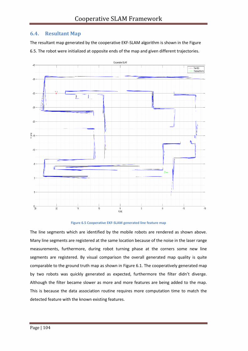
Cooperative SLAM Framework
Page | 104
6.4. Resultant Map
The resultant map generated by the cooperative EKF-SLAM algorithm is shown in the Figure
6.5. The robot were initialized at opposite ends of the map and given different trajectories.
Figure 6.5 Cooperative EKF-SLAM generated line feature map
The line segments which are identified by the mobile robots are rendered as shown above.
Many line segments are registered at the same location because of the noise in the laser range
measurements, furthermore, during robot turning phase at the corners some new line
segments are registered. By visual comparison the overall generated map quality is quite
comparable to the ground truth map as shown in Figure 6.1. The cooperatively generated map
by two robots was quickly generated as expected, furthermore the filter didn’t diverge.
Although the filter became slower as more and more features are being added to the map.
This is because the data association routine requires more computation time to match the
detected feature with the known existing features.
Cooperative SLAM Framework
Page | 105
6.5. Summary
In this chapter the cooperative EKF-SLAM algorithm experiment and its results are discussed.
To validate the cooperative EKF-SLAM algorithm a simulation environment is setup using
USARSim setup. The simulation setup not only provides a ground truth data for result
comparison but also it provides a fast method to experiment the Cooperative SLAM
algorithms. To autonomously drive the robot in the modeled static environment a way point
navigation controller is also implemented.
The navigation controller moves the robot from the current robot pose to a target pose in
three steps. First by rotating toward the goal, then move toward the goal and finally rotation
toward the target orientation.
The state vector is composed in such a way that searching for robot pose or features remains
faster. The other characteristics of the line segments such as end points, length are stored in a
separate list. The order of the line segments in the state vector is kept the same as in the state
vector. Overlapping line segments are fused together while non-overlapping line segments
with same parameters are detected also to avoid false data association. And finally the
resultant map generated by the cooperative SLAM algorithm is discussed.
Cooperative SLAM Framework
Page | 106
Chapter 7.
Discussion
In this thesis, a cooperative SLAM framework based on extended Kalman filter is formularized.
Furthermore a cooperative software framework for heterogeneous mobile robots is
developed. The background study related to the SLAM, the state of the art SLAM algorithms
and the cooperative mobile robot simulation environments has been covered and the core
topics for the SLAM implementations are discussed. SLAM is performed where a priori map of
the environment is not available and it is not possible to use global positioning devices to find
the accurate position of the mobile robot.
The proposed cooperative SLAM framework can use multiple mobile robots equipped with 2D
and 3D range sensors for building the environment map assuming initial relative pose between
mobile robots is known. The framework can also provide a general purpose interface to
configure, control and manage a team of mobile robots and the sensor data.
In chapter 1 the motivation, research work scope and the related works regarding the SLAM
problem and its solutions are discussed. In Chapter 2 Odometry based motion model for the
differential drive mobile robots and the range sensor based observation model for mobile
robots are discussed. Extended Kalman filter is used as the core estimation engine because of
its simplicity for the Cooperative SLAM problem. The robot pose estimation is critical to the
localization and mapping, therefore, two novel data fusion strategies are proposed. The
geometric feature based map is selected for research work because it model the environment
into the high level features which not only reduces the memory requirements but also helpful
for semantic understanding of the environment.
Chapter 3 discusses the major modules which are necessary for successful implementation for
the SLAM. Different algorithms regarding range sensor data segmentation, feature estimation,
data association, map update and new feature augmentation in to the existing map are also
discussed. Non-Linear least square estimation technique is used to extract the 2D geometric
lines from the range data. The non-linear estimate is not biased toward the minimization of
error with respect to x or y axis, instead it minimizes the error of the measured points with
respect to the linear distance perpendicular to the estimated line. Two algorithms namely
RANSAC and Hough transformation are used to extract the 3D geometric planes from the
Cooperative SLAM Framework
Page | 107
point cloud. Hough transformation estimated planes more reliably while the RANSAC
algorithm was comparatively little faster than Hough transformation to extract the planes.
In Chapter 4 a mathematical cooperative SLAM formulation is described based on the
extended Kalman filter. The cooperative SLAM assumes that the initial relative pose among
the mobile robot is known. Each time when the estimated feature associate with the existing
feature, the two features coordinates are fused. For example in case of the 2D line feature, the
end coordinates the extracted line and the existing lines are merged in such a way that the
longest line is archived.
In Chapter 5 the software framework which is used to control, configure and manage the
heterogeneous robots is discussed. Furthermore, for the rapid development of the algorithm a
simulation environment which can be interfaced to the framework is also described. The
framework is a step toward the standardization of the interfaces used for a team of mobile
robots. Ground coordinator provides a general purpose interface to communicate with the
mobile robots and manage their sensor data. The communication protocol provides a format
which can be used to implement customized communication packets. The firmware is also
designed in a modular way so that the customized modules can be developed and added later
on. Each module implements some communication commands and reports protocol which are
essential for configuring the module remotely. Similarly the Hardware board is designed to be
as general purpose as possible so that hardware sensors can be attached as required. A
simulation environment based on the USARSim is also introduced for the rapid development
and prototyping of SLAM algorithms.
Chapter 6 discussed the results of the cooperative SLAM experiment. Two ground mobile
robots are simulated in the USARSim. Both robots are attached with a 2D laser range scanner
and odometry. Both robots data is acquired by the coordinator software and then a combined
map is generated by the mathematical framework similar to as discussed in chapter 4.
7.1. Outlook
Apart from different algorithms used for the individual components of the SLAM the output of
implemented SLAM solution depends on the choice of the sensor used for the environment
observation. Few draw backs regarding different range sensors are as follows. Range sensors
such as TOF cameras and RGB-D cameras are sensitive to sunlight and distance to target
object. TOF cameras are also sensitive to color of the surface and they are too noisy and
sparse to build the map in outdoor environment. Laser sensors measurements are corrupted
Cooperative SLAM Framework
Page | 108
by the glass surface. Range measurement using stereo cameras can’t be used in very
homogenous environments and on mirror surfaces. The laser range finder is the most accurate
sensor for mapping in both indoor and outdoor environment.
Feature based SLAM performance heavily depends also on data association technology. The
simplest is the nearest neighbor approach. Neira proposed a joint compatibility approach to
consider correlation among map features. For a feature map based SLAM approach a more
sophisticated strategy is necessary such as octree.
7.2. Contributions
Following are the contribution of this thesis
Overview of the SLAM algorithms.
Overview of the start of art mobile robotics simulation software’s.
Two novel mobile robot’s pose estimation approach
o Multi-sensor data fusion based on Indirect Kalman Filter
o Data fusion between Gyroscope and Stereo vision.
Grid map and feature map creation utilities.
Development of the mathematical cooperative SLAM formulization based on extended
Kalman filter.
Implementation of plane extraction and geometric map building technique toward
SLAM implementation.
Sensor data fusion methodologies based on Kalman filtering.
Novel cooperative SLAM framework for controlling, configuring and managing a team
of mobile robots
Development of standard communication interfaces for cooperating among team of
mobile robots.
Cooperative SLAM Framework
Page | 109
7.3. Future Works
Despite of two decade research the SLAM problem is not fully solved. The SLAM is solved for
indoor, structured, static and small environment. For outdoor and dynamic environment it still
poses many challenges, furthermore the problem of loop closure and data associations are still
required research works. The solutions to cooperative SLAM among many robots are still
missing the map fusion part in case the initial relative robot pose are unknown. There is also a
need of methods which run in real time with the available memory even for large maps with
limited computational power.
Various other issues need to be investigated such as map complexity, dynamic environment
and computational requirements. The map fusion when the relative pose is not known also
need to be investigated. At the moment the robust SLAM approach for single robot is
GMapping, also known as Rao-Blackwellised particle filter, which required an accurate laser
range finder and odometry data. Rao-Blackwellised filter is an efficient SLAM implementation
which scales logarithmically with the number of landmarks. It uses an EKF of features estimate
and a PF for robot state. The resampling process is crucial for PF. GMapping is the state of the
art implementation of the SLAM algorithm. The research work can be extended to incorporate
particle filter and extended Kalman filter like GMapping.
Particle filter approach when implemented on GPU for cooperative SLAM problem can help to
overcome the computational requirement which arises because of handling very large state
vectors, the computational time increase quadratically with the number of features in the
map, and multiple hypotheses about robot pose. Particle filters is implemented on a GPU
using CUDA because of the presence of the inherited parallelism. The particle filter approach
also helps because it can handle non-linear robot motion and observation model where EKF
fails if the non-linarites are too strong. It is robust against wrong data association because of
resampling step and the computation cost is proportional to the number of particles.
A TOF camera with higher field of view and resolution can also be used for further
investigation.
In the case where GT data is not available, one could evaluate his method based on the
qualitative impression of the resulting map. In the case when the blueprint of the experiment
environment is available even the direct comparison among different algorithms is difficult as
different publications are evaluated with different dataset. The rawseeds project [107] funded
by European Union is an effort to provide GT data for SLAM algorithms.
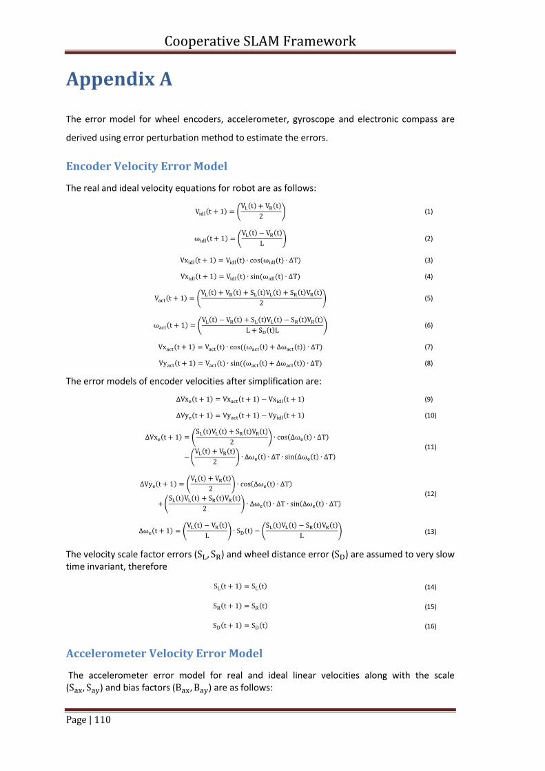
Cooperative SLAM Framework
Page | 110
Appendix A
The error model for wheel encoders, accelerometer, gyroscope and electronic compass are
derived using error perturbation method to estimate the errors.
Encoder Velocity Error Model
The real and ideal velocity equations for robot are as follows:
( ) ( ( ) ( )
) (1)
( ) ( ( ) ( )
) (2)
( ) ( ) ( ( ) ) (3)
( ) ( ) ( ( ) ) (4)
( ) ( ( ) ( ) ( ) ( ) ( ) ( )
) (5)
( ) ( ( ) ( ) ( ) ( ) ( ) ( )
( ) ) (6)
( ) ( ) (( ( ) ( )) ) (7)
( ) ( ) (( ( ) ( )) ) (8)
The error models of encoder velocities after simplification are:
( ) ( ) ( ) (9)
( ) ( ) ( ) (10)
( ) ( ( ) ( ) ( ) ( )
) ( ( ) )
( ( ) ( )
) ( ) ( ( ) )
(11)
( ) ( ( ) ( )
) ( ( ) )
( ( ) ( ) ( ) ( )
) ( ) ( ( ) )
(12)
( ) ( ( ) ( )
) ( ) (
( ) ( ) ( ) ( )
) (13)
The velocity scale factor errors ( ) and wheel distance error ( ) are assumed to very slow time invariant, therefore
( ) ( ) (14)
( ) ( ) (15)
( ) ( ) (16)
Accelerometer Velocity Error Model
The accelerometer error model for real and ideal linear velocities along with the scale ( ) and bias factors ( ) are as follows:
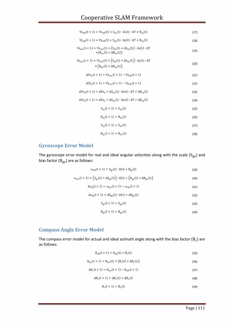
Cooperative SLAM Framework
Page | 111
( ) ( ) ( ) ( ) ( ) (17)
( ) ( ) ( ) ( ) ( ) (18)
( ) ( ) ( ( ) ( )) ( )
( ( ) ( )) (19)
( ) ( ) . ( ) ( )/ ( )
. ( ) ( )/ (20)
( ) ( ) ( ) (21)
( ) ( ) ( ) (22)
( ) ( ) ( ) ( ) (23)
( ) ( ) ( ) ( ) (24)
( ) ( ) (25)
( ) ( ) (26)
( ) ( ) (27)
( ) ( ) (28)
Gyroscope Error Model
The gyroscope error model for real and ideal angular velocities along with the scale ( ) and
bias factor ( ) are as follows:
( ) ( ) ( ) ( ) (29)
( ) . ( ) ( )/ ( ) . ( ) ( )/ (30)
( ) ( ) ( ) (31)
( ) ( ) ( ) ( ) (32)
( ) ( ) (33)
( ) ( ) (34)
Compass Angle Error Model
The compass error model for actual and ideal azimuth angle along with the bias factor ( ) are as follows:
( ) ( ) ( ) (35)
( ) ( ) ( ( ) ( )) (36)
( ) ( ) ( ) (37)
( ) ( ) ( ) (38)
( ) ( ) (39)
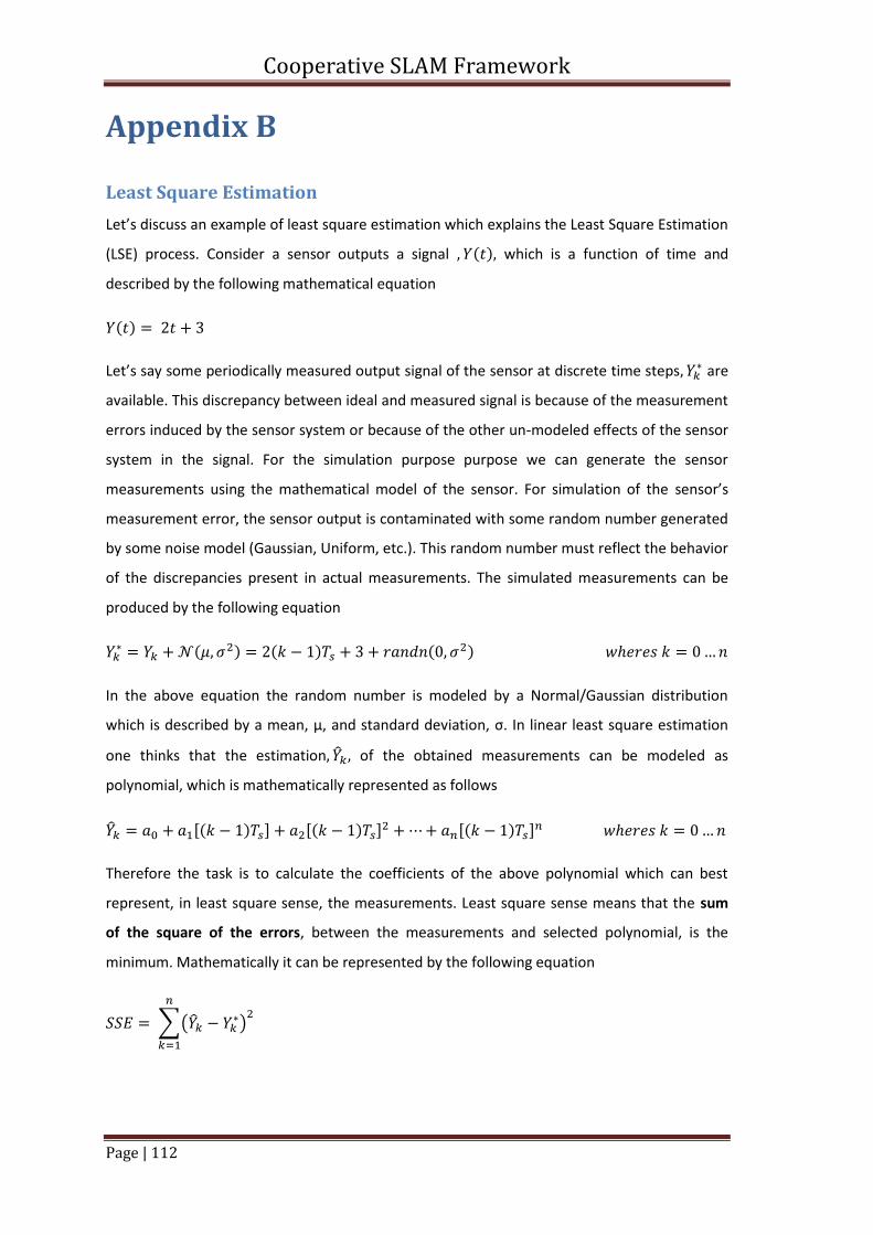
Cooperative SLAM Framework
Page | 112
Appendix B
Least Square Estimation
Let’s discuss an example of least square estimation which explains the Least Square Estimation
(LSE) process. Consider a sensor outputs a signal ( ) which is a function of time and
described by the following mathematical equation
( )
Let’s say some periodically measured output signal of the sensor at discrete time steps are
available. This discrepancy between ideal and measured signal is because of the measurement
errors induced by the sensor system or because of the other un-modeled effects of the sensor
system in the signal. For the simulation purpose purpose we can generate the sensor
measurements using the mathematical model of the sensor. For simulation of the sensor’s
measurement error, the sensor output is contaminated with some random number generated
by some noise model (Gaussian, Uniform, etc.). This random number must reflect the behavior
of the discrepancies present in actual measurements. The simulated measurements can be
produced by the following equation
(
) ( ) ( )
In the above equation the random number is modeled by a Normal/Gaussian distribution
which is described by a mean, µ, and standard deviation, σ. In linear least square estimation
one thinks that the estimation of the obtained measurements can be modeled as
polynomial, which is mathematically represented as follows
,( ) - ,( ) - ,( ) -
Therefore the task is to calculate the coefficients of the above polynomial which can best
represent, in least square sense, the measurements. Least square sense means that the sum
of the square of the errors, between the measurements and selected polynomial, is the
minimum. Mathematically it can be represented by the following equation
∑( )
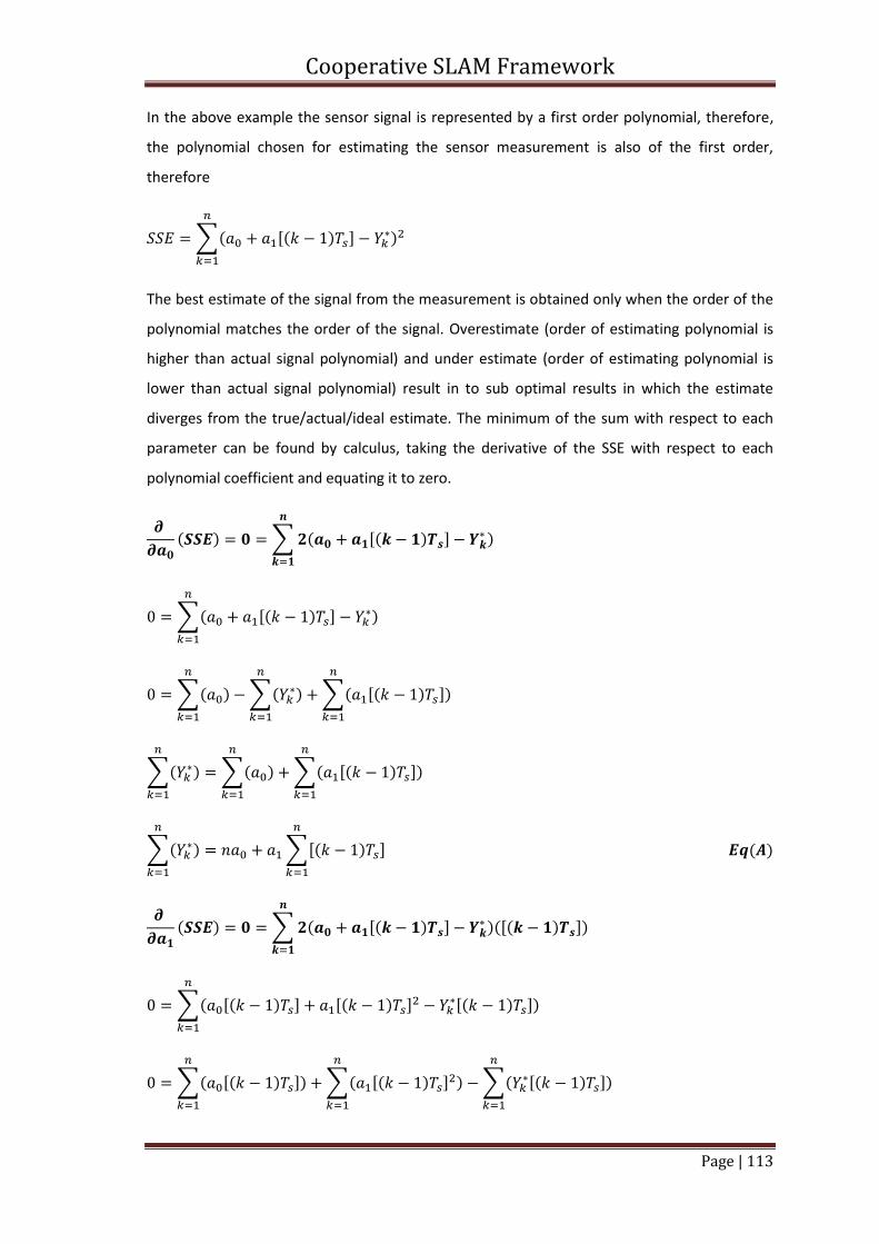
Cooperative SLAM Framework
Page | 113
In the above example the sensor signal is represented by a first order polynomial, therefore,
the polynomial chosen for estimating the sensor measurement is also of the first order,
therefore
∑( ,( ) - )
The best estimate of the signal from the measurement is obtained only when the order of the
polynomial matches the order of the signal. Overestimate (order of estimating polynomial is
higher than actual signal polynomial) and under estimate (order of estimating polynomial is
lower than actual signal polynomial) result in to sub optimal results in which the estimate
diverges from the true/actual/ideal estimate. The minimum of the sum with respect to each
parameter can be found by calculus, taking the derivative of the SSE with respect to each
polynomial coefficient and equating it to zero.
( ) ∑ ( ,( ) -
)
∑( ,( ) - )
∑( )
∑( )
∑( ,( ) -)
∑( )
∑( )
∑( ,( ) -)
∑( )
∑,( ) -
( )
( ) ∑ ( ,( ) -
)(,( ) -)
∑( ,( ) - ,( ) -
,( ) -)
∑( ,( ) -)
∑( ,( ) - )
∑( ,( ) -)
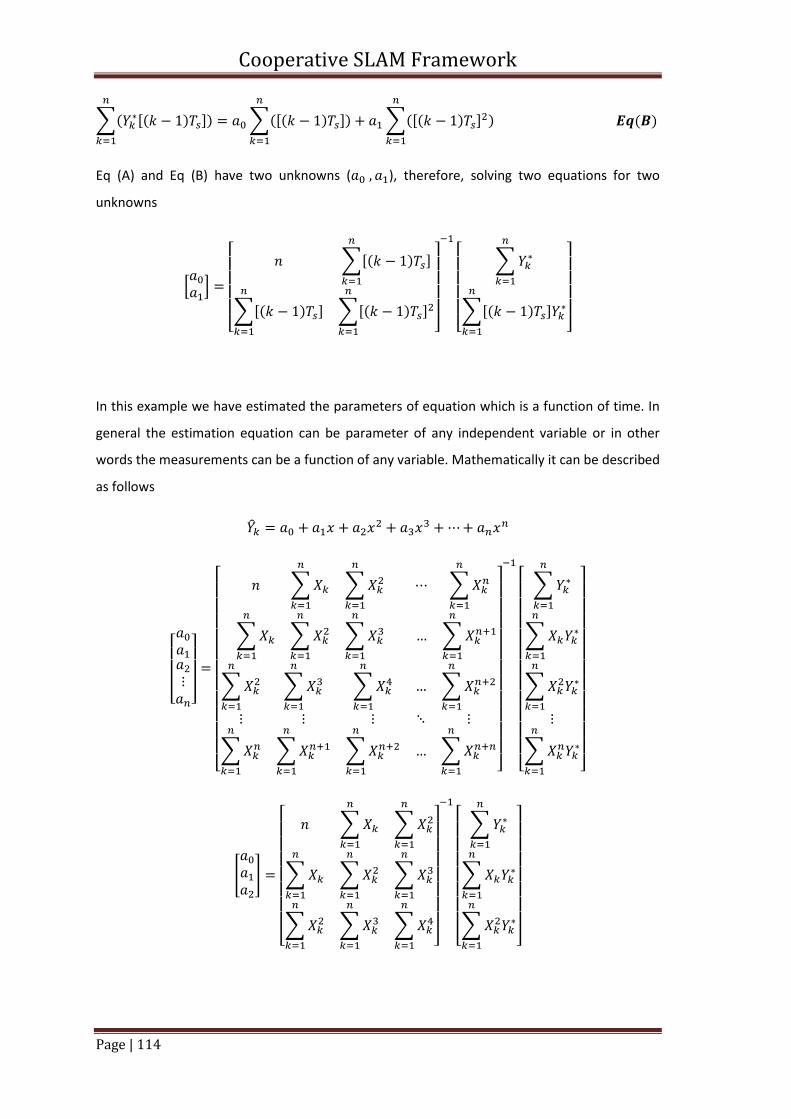
Cooperative SLAM Framework
Page | 114
∑( ,( ) -)
∑(,( ) -)
∑(,( ) - )
( )
Eq (A) and Eq (B) have two unknowns ( ), therefore, solving two equations for two
unknowns
0 1
[ ∑,( ) -
∑,( ) -
∑,( ) -
]
[ ∑
∑,( ) -
]
In this example we have estimated the parameters of equation which is a function of time. In
general the estimation equation can be parameter of any independent variable or in other
words the measurements can be a function of any variable. Mathematically it can be described
as follows
[ ]
[ ∑
∑
∑
∑
∑
∑
∑
∑
∑
∑
∑
∑
∑
∑
∑
]
[ ∑
∑
∑
∑
]
[
]
[ ∑
∑
∑
∑
∑
∑
∑
∑
]
[ ∑
∑
∑
]
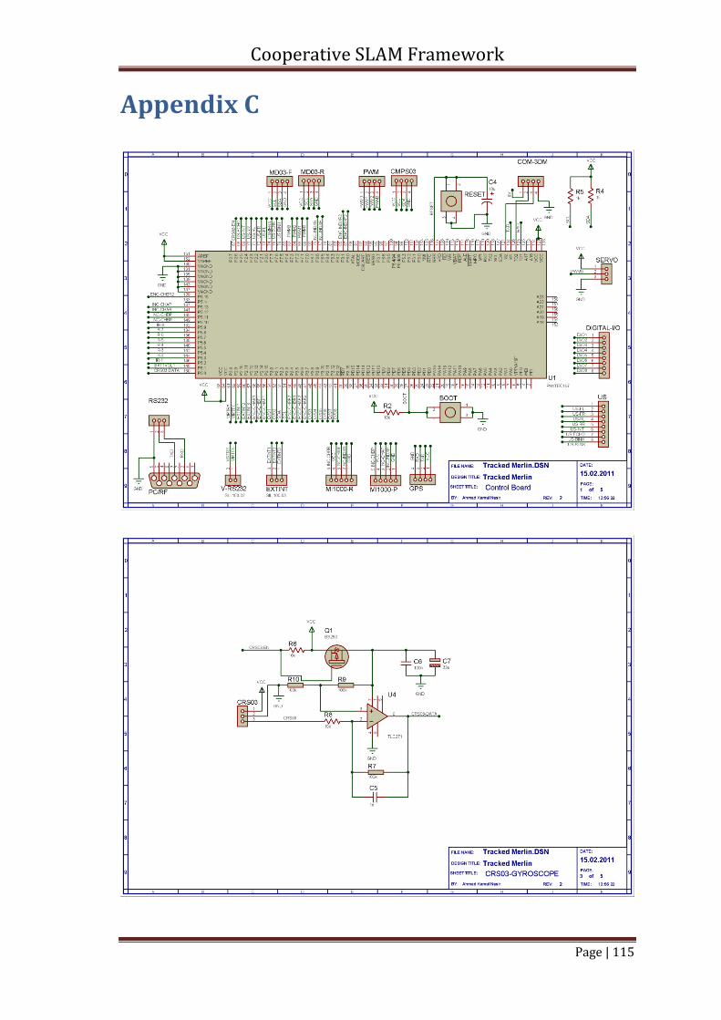
Cooperative SLAM Framework
Page | 115
Appendix C
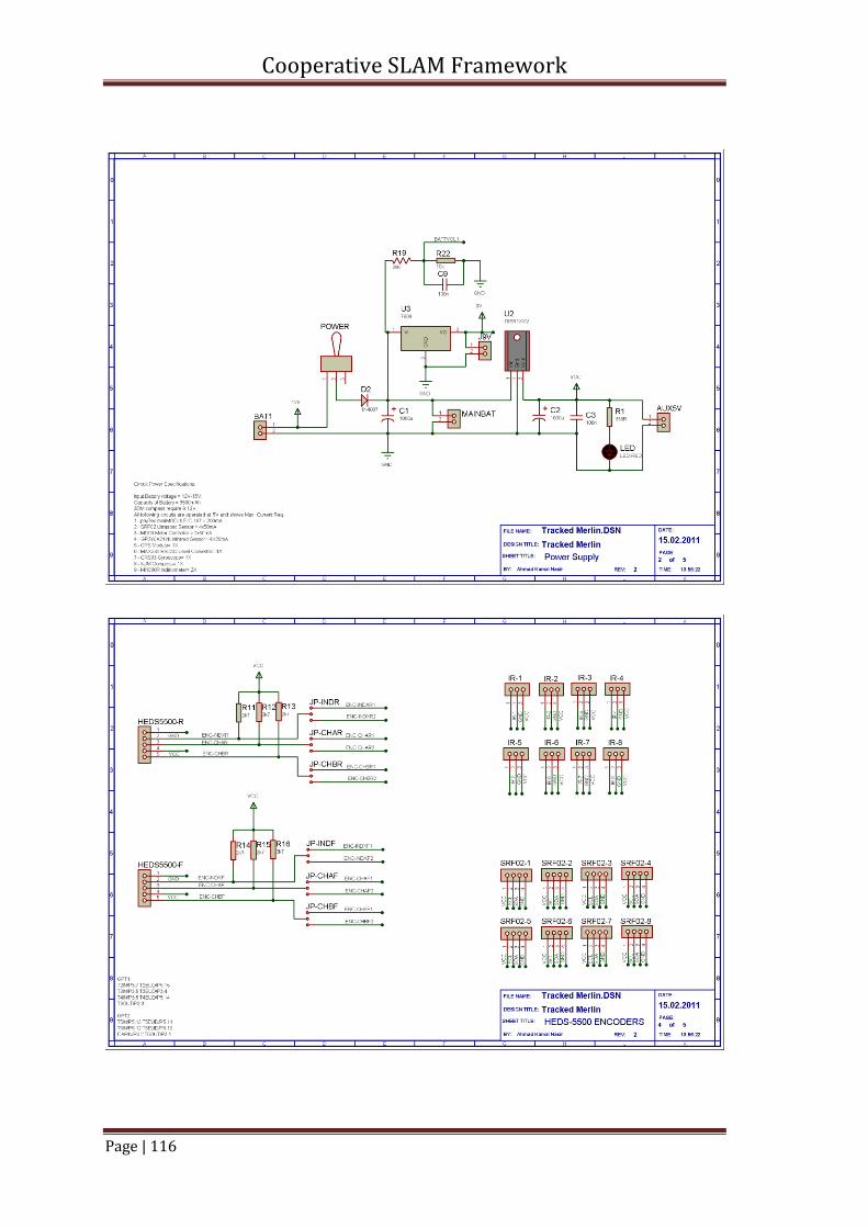
Cooperative SLAM Framework
Page | 116
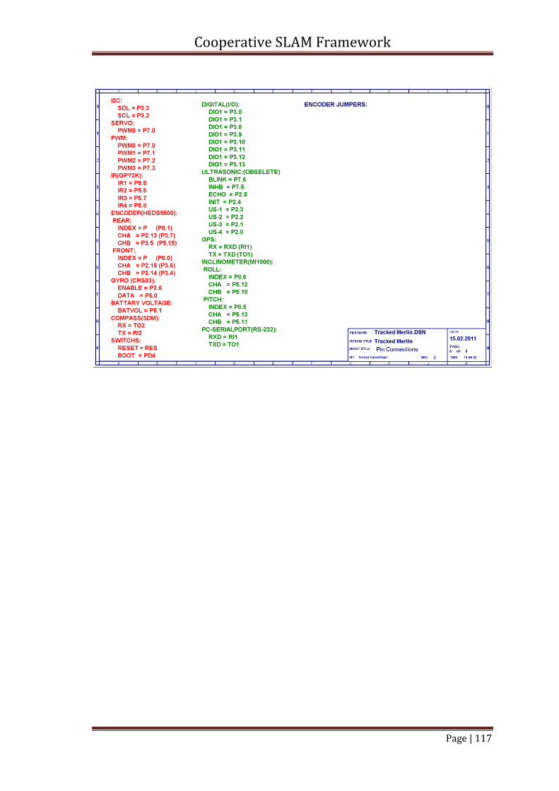
Cooperative SLAM Framework
Page | 117
Cooperative SLAM Framework
Page | 118
Appendix D
Create an C# based TCP/IP Client to communicate with a simulated
robot in USARSim
This guide will help to create an application in C# which can communicate with simulated
robots in USARSim environment. USARSim provides a simulation environment for robots.
Many commercial ground, aerial robot models environment maps and virtual sensors and
actuators are included.
Setting up a Simulation Environment
This guide assumes that we are using a Windows-7 operating system with 8GB Ram and a
graphics card. After we have downloaded and installed the Dec-2011 UDK release, we have to
download the USARSim v1.3 and extract all the files in the same directory where we have
installed the UDK. This process will copy the necessary maps, models and configuration files at
the desired location. After extracting, e.g. the destination path C:\UDK\UDK-2011-12\, the
USARSim related files one can execute the make file in the base UDK directory to compile the
simulation entities.
Running Simulation Environment
After the simulation environment is setup we can run any one of the provided map in the
C:\UDK\UDK-2011-12\USARRunMaps environment, a batch file which will load a map and run
the game server. If everything was correct then the game server is started at the local machine
(127.0.0.1:3000) and load the specified map. Initially the map is without any robots. The
robots are spawned as bots in the game map. We can execute the game related commands by
typing them at the command terminal (Appears by pressing TAB).
Communication with game engine
After the game engine is started and running we can send commands to spawn the robots and
communicate robot sensors and actuators data. The communication between the game server
and a client (user program) must be by using TCP/IP communication protocol format. The user
must first establish a TCP/IP connection to already game server (IPAddress:Port) and then the
navigation and actuators commands can be sent and sensors data can be received. For the
detailed description of the command formats please refer to the documentation of the
USARSim. For the communication, sensors parameters, and robots sensors settings look at the
C:\UDK\UDK-2011-12\UDKGame\Config\DefaultUSAR.ini.
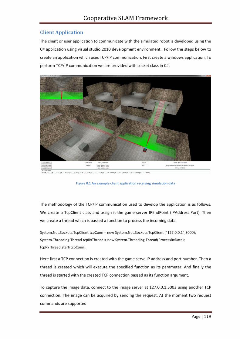
Cooperative SLAM Framework
Page | 119
Client Application
The client or user application to communicate with the simulated robot is developed using the
C# application using visual studio 2010 development environment. Follow the steps below to
create an application which uses TCP/IP communication. First create a windows application. To
perform TCP/IP communication we are provided with socket class in C#.
Figure 0.1 An example client application receiving simulation data
The methodology of the TCP/IP communication used to develop the application is as follows.
We create a TcpClient class and assign it the game server IPEndPoint (IPAddress:Port). Then
we create a thread which is passed a function to process the incoming data.
System.Net.Sockets.TcpClient tcpConn = new System.Net.Sockets.TcpClient (“127.0.0.1”,3000);
System.Threading.Thread tcpRxThread = new System.Threading.Thread(ProcessRxData);
tcpRxThread.start(tcpConn);
Here first a TCP connection is created with the game serve IP address and port number. Then a
thread is created which will execute the specified function as its parameter. And finally the
thread is started with the created TCP connection passed as its function argument.
To capture the image data, connect to the image server at 127.0.0.1:5003 using another TCP
connection. The image can be acquired by sending the request. At the moment two request
commands are supported
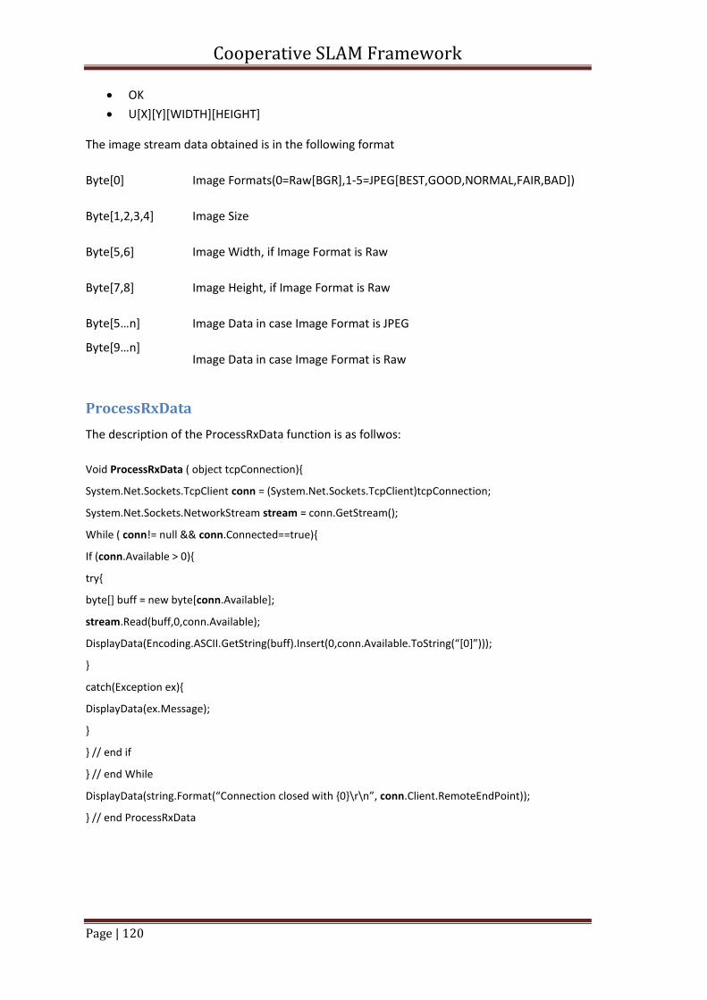
Cooperative SLAM Framework
Page | 120
OK
U[X][Y][WIDTH][HEIGHT]
The image stream data obtained is in the following format
Byte[0] Image Formats(0=Raw[BGR],1-5=JPEG[BEST,GOOD,NORMAL,FAIR,BAD])
Byte[1,2,3,4] Image Size
Byte[5,6] Image Width, if Image Format is Raw
Byte[7,8] Image Height, if Image Format is Raw
Byte*5…n+
Byte*9…n+
Image Data in case Image Format is JPEG
Image Data in case Image Format is Raw
ProcessRxData
The description of the ProcessRxData function is as follwos:
Void ProcessRxData ( object tcpConnection){
System.Net.Sockets.TcpClient conn = (System.Net.Sockets.TcpClient)tcpConnection;
System.Net.Sockets.NetworkStream stream = conn.GetStream();
While ( conn!= null && conn.Connected==true){
If (conn.Available > 0){
try{
byte[] buff = new byte[conn.Available];
stream.Read(buff,0,conn.Available);
DisplayData(Encoding.ASCII.GetString(buff).Insert(0,conn.Available.ToString(“*0+”)));
}
catch(Exception ex){
DisplayData(ex.Message);
}
} // end if
} // end While
DisplayData(string.Format(“Connection closed with ,0-\r\n”, conn.Client.RemoteEndPoint));
} // end ProcessRxData
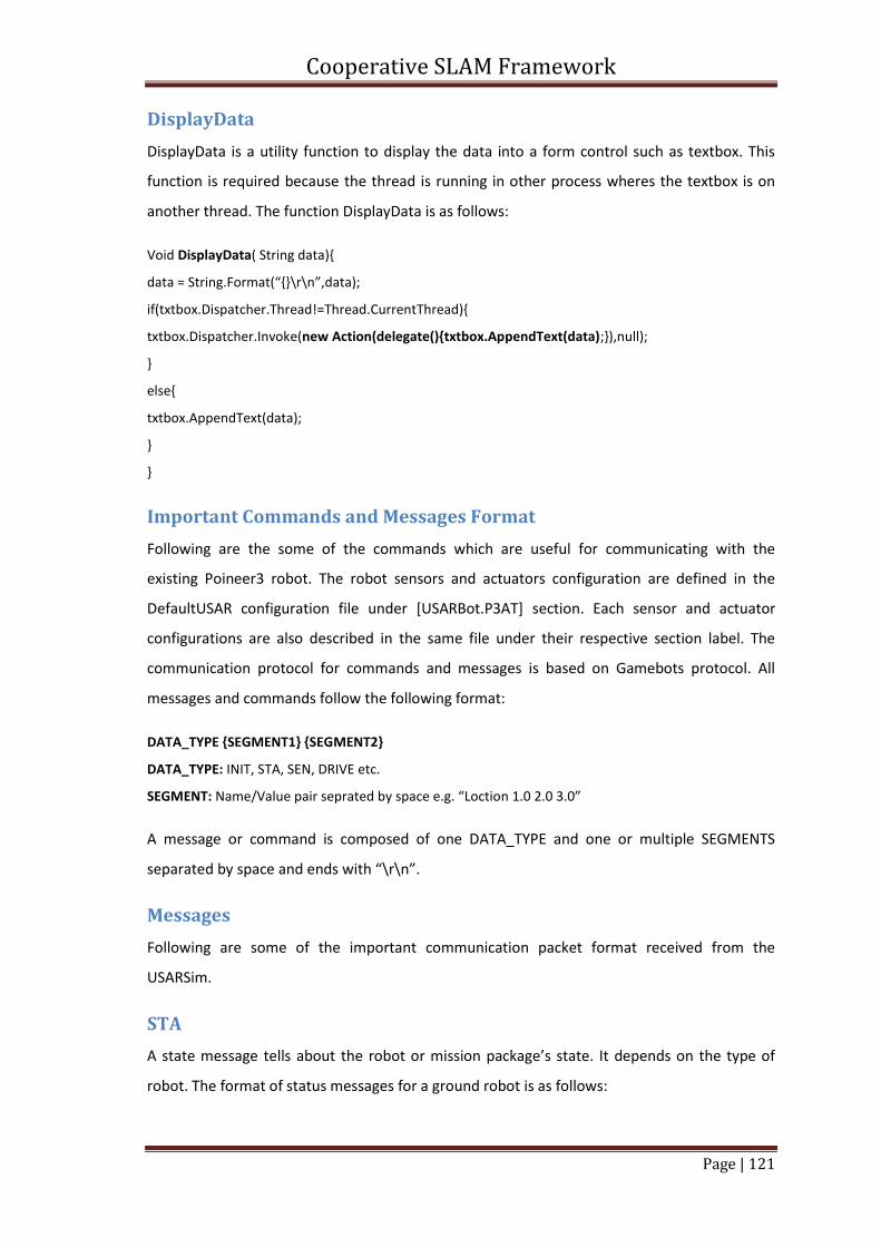
Cooperative SLAM Framework
Page | 121
DisplayData
DisplayData is a utility function to display the data into a form control such as textbox. This
function is required because the thread is running in other process wheres the textbox is on
another thread. The function DisplayData is as follows:
Void DisplayData( String data){
data = String.Format(“,-\r\n”,data);
if(txtbox.Dispatcher.Thread!=Thread.CurrentThread){
txtbox.Dispatcher.Invoke(new Action(delegate(){txtbox.AppendText(data);}),null);
}
else{
txtbox.AppendText(data);
}
}
Important Commands and Messages Format
Following are the some of the commands which are useful for communicating with the
existing Poineer3 robot. The robot sensors and actuators configuration are defined in the
DefaultUSAR configuration file under [USARBot.P3AT] section. Each sensor and actuator
configurations are also described in the same file under their respective section label. The
communication protocol for commands and messages is based on Gamebots protocol. All
messages and commands follow the following format:
DATA_TYPE {SEGMENT1} {SEGMENT2}
DATA_TYPE: INIT, STA, SEN, DRIVE etc.
SEGMENT: Name/Value pair seprated by space e.g. “Loction 1.0 2.0 3.0”
A message or command is composed of one DATA_TYPE and one or multiple SEGMENTS
separated by space and ends with “\r\n”.
Messages
Following are some of the important communication packet format received from the
USARSim.
STA
A state message tells about the robot or mission package’s state. It depends on the type of
robot. The format of status messages for a ground robot is as follows:
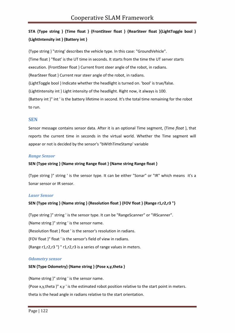
Cooperative SLAM Framework
Page | 122
STA {Type string } {Time float } {FrontSteer float } {RearSteer float }{LightToggle bool }
{LightIntensity int } {Battery int }
{Type string } "string' describes the vehicle type. In this case: "GroundVehicle".
{Time float } "float' is the UT time in seconds. It starts from the time the UT server starts
execution. {FrontSteer float } Current front steer angle of the robot, in radians.
{RearSteer float } Current rear steer angle of the robot, in radians.
{LightToggle bool } Indicate whether the headlight is turned on. 'bool' is true/false.
{LightIntensity int } Light intensity of the headlight. Right now, it always is 100.
{Battery int }" int ' is the battery lifetime in second. It's the total time remaining for the robot
to run.
SEN
Sensor message contains sensor data. After it is an optional Time segment, {Time float }, that
reports the current time in seconds in the virtual world. Whether the Time segment will
appear or not is decided by the sensor's "bWithTimeStamp' variable
Range Sensor
SEN {Type string } {Name string Range float } {Name string Range float }
{Type string }" string ' is the sensor type. It can be either "Sonar" or "IR" which means it's a
Sonar sensor or IR sensor.
Laser Sensor
SEN {Type string } {Name string } {Resolution float } {FOV float } {Range r1,r2,r3 "}
{Type string }" string ' is the sensor type. It can be "RangeScanner" or "IRScanner".
{Name string }" string ' is the sensor name.
{Resolution float } float ' is the sensor's resolution in radians.
{FOV float }" float ' is the sensor's field of view in radians.
{Range r1,r2,r3 "} " r1,r2,r3 is a series of range values in meters.
Odometry sensor
SEN {Type Odometry} {Name string } {Pose x,y,theta }
{Name string }" string ' is the sensor name.
{Pose x,y,theta }" x,y ' is the estimated robot position relative to the start point in meters.
theta is the head angle in radians relative to the start orientation.
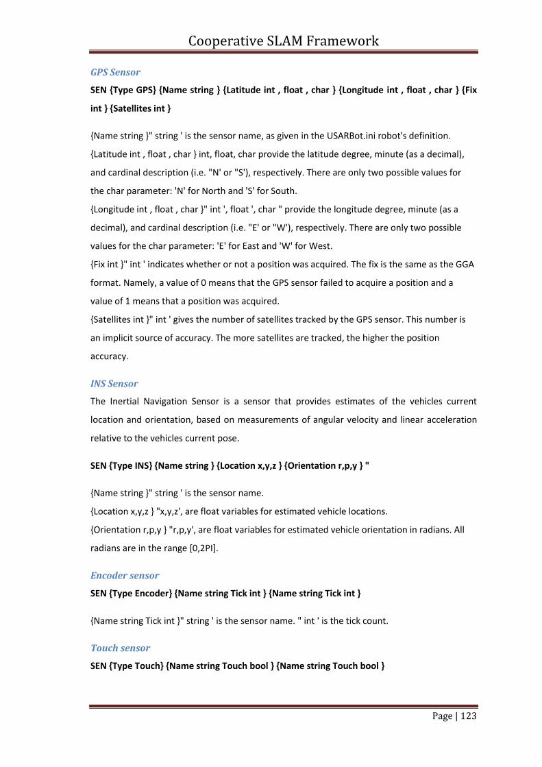
Cooperative SLAM Framework
Page | 123
GPS Sensor
SEN {Type GPS} {Name string } {Latitude int , float , char } {Longitude int , float , char } {Fix
int } {Satellites int }
{Name string }" string ' is the sensor name, as given in the USARBot.ini robot's definition.
{Latitude int , float , char } int, float, char provide the latitude degree, minute (as a decimal),
and cardinal description (i.e. "N' or "S'), respectively. There are only two possible values for
the char parameter: 'N' for North and 'S' for South.
{Longitude int , float , char }" int ', float ', char " provide the longitude degree, minute (as a
decimal), and cardinal description (i.e. "E' or "W'), respectively. There are only two possible
values for the char parameter: 'E' for East and 'W' for West.
{Fix int }" int ' indicates whether or not a position was acquired. The fix is the same as the GGA
format. Namely, a value of 0 means that the GPS sensor failed to acquire a position and a
value of 1 means that a position was acquired.
{Satellites int }" int ' gives the number of satellites tracked by the GPS sensor. This number is
an implicit source of accuracy. The more satellites are tracked, the higher the position
accuracy.
INS Sensor
The Inertial Navigation Sensor is a sensor that provides estimates of the vehicles current
location and orientation, based on measurements of angular velocity and linear acceleration
relative to the vehicles current pose.
SEN {Type INS} {Name string } {Location x,y,z } {Orientation r,p,y } "
{Name string }" string ' is the sensor name.
{Location x,y,z } "x,y,z', are float variables for estimated vehicle locations.
{Orientation r,p,y } "r,p,y', are float variables for estimated vehicle orientation in radians. All
radians are in the range [0,2PI].
Encoder sensor
SEN {Type Encoder} {Name string Tick int } {Name string Tick int }
{Name string Tick int }" string ' is the sensor name. " int ' is the tick count.
Touch sensor
SEN {Type Touch} {Name string Touch bool } {Name string Touch bool }
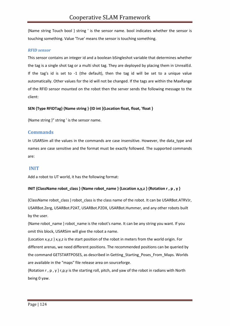
Cooperative SLAM Framework
Page | 124
{Name string Touch bool } string ' is the sensor name. bool indicates whether the sensor is
touching something. Value 'True' means the sensor is touching something.
RFID sensor
This sensor contains an integer id and a boolean bSingleshot variable that determines whether
the tag is a single shot tag or a multi shot tag. They are deployed by placing them in UnrealEd.
If the tag's id is set to -1 (the default), then the tag id will be set to a unique value
automatically. Other values for the id will not be changed. If the tags are within the MaxRange
of the RFID sensor mounted on the robot then the server sends the following message to the
client:
SEN {Type RFIDTag} {Name string } {ID int }{Location float, float, 'float }
{Name string }" string ' is the sensor name.
Commands
In USARSim all the values in the commands are case insensitive. However, the data_type and
names are case sensitive and the format must be exactly followed. The supported commands
are:
INIT
Add a robot to UT world, it has the following format:
INIT {ClassName robot_class } {Name robot_name } {Location x,y,z } {Rotation r , p , y }
{ClassName robot_class } robot_class is the class name of the robot. It can be USARBot.ATRVJr,
USARBot.Zerg, USARBot.P2AT, USARBot.P2DX, USARBot.Hummer, and any other robots built
by the user.
{Name robot_name } robot_name is the robot's name. It can be any string you want. If you
omit this block, USARSim will give the robot a name.
{Location x,y,z } x,y,z is the start position of the robot in meters from the world origin. For
different arenas, we need different positions. The recommended positions can be queried by
the command GETSTARTPOSES, as described in Getting_Starting_Poses_From_Maps. Worlds
are available in the "maps" file release area on sourceforge.
{Rotation r , p , y } r,p,y is the starting roll, pitch, and yaw of the robot in radians with North
being 0 yaw.
Cooperative SLAM Framework
Page | 125
DRIVE
Control the Robot. There are seven kinds of control command. The first kind controls the left
and right side wheels of a skid steered robot. The second kind controls the front and rear
wheels of an Ackerman steered robot. The third kind controls an underwater robot. The fourth
kind controls an aerial vehicle. The fifth kind controls the wheels of an OmniDrive robot. The
sixth kind controls a specified joint of the robot. The seventh kind controls the angle of
multiple joints of a robot, which is convenient for flipper, leg, and arm control.
DRIVE {Left float } {Right float } {Normalized bool } {Light bool } {Flip bool }
{Left float } float is spin speed for the left side wheels. If we are using normalized values, the
value range is -100 to 100 and corresponds to the robot's minimum and maximum spin speed.
If we use absolute values, the value will be the real spin speed in radians per second.
{Right float } Same as above except the values affect the right side wheels.
{Normalized bool } Indicates whether we are using normalized values or not. The default value
is "False' which means absolute values are used to control wheel spin speed.
{Light bool } bool ' is whether turn on or turn off the headlight. The possible values are
True/False.
{Flip bool } If a robot rolls over or otherwise tips off of its wheels, this will "right" the robot. If
bool ' is True, this command will flip the robot to its "wheels down' position.
Cooperative SLAM Framework
Page | 126
Appendix E
Simulation of Map Building in ROS with Mobile Robots Equipped with
Odometry and Laser Range Scanner
A simulation world is created in Stage (2D simulation system). The simulation environment
consists of a map and two differential drive mobile robots. The robots are equipped with a
laser range scan system and an odometry system. The map is in fact a top view (plan) of the
building which is stored as a PNG file format. The simulation world file (simulation.world) of
the Stage simulation system depends on the robot model files; TOM3D.inc, Trackedmerlin.inc
and a map file (Map.inc).
It is assumed that the following packages are already installed on the ROS system:
Stage
Rviz
Gmapping Furthermore, eclipse indigo c/c++ IDE for linux developers is also installed on the development
system. The ROS system is installed under Ubuntu 10.04.4 is electric desktop distribution
which is fully installed. The stage world files along with its dependent model files are displayed
at the end of this document.
The stage simulation system is publishing odometry and laser scanner data on /odom and
/base_scan topics. While to control the movement of the robot another topic it is subscribed
to a topic names cmd_vel. To communicate with the simulated system a ROS package has
been created into as follows:
roscreate-pkg simulation roscpp stage std_msgs nav_msgs sensor_msgs geometry_msgs
cd simulation
make eclipse-project
Then import the above created project into eclipse and add the controller.cpp file which is
displayed at the end of this document. After that modify the CMakeLists.txt file, at the end of
the file write the following line rosbuild_add_executable(controller src/controller.cpp). Build
the eclipse project.
After successful compilation of the package. Create a launch file as shown at the end of the
document. This launch file will run the roscore and load the stage simulation system along
with the world file and also run the controller node which will communicate with the relevant
Cooperative SLAM Framework
Page | 127
topics to interact with the simulation. To create the map of the simulated envriornment run
the following command at the command prompt:
rosrun gmapping slam_gmapping scan:=base_scan
To save a snapshot of the mapped environment one can use the following command
rosrun map_server map_saver
To visualize the map building process we need the rviz package to be installed. To run the rviz
system type the following command at the terminal
rosrun rviz rviz
When the rviz system is successfully launched then add a map display into it and set its node
to /map which is being published by the gmapping system. One can record also the simulation
experiment by the following ros command
rosbag record –o dataset /odom /base_pose_ground_truth /base_scan /cmd_vel
To use the exsisting dataset (bag file) use the following commands
rosparam set /use_set_time true
rosbag play dataset.bag
Cooperative SLAM Framework
Page | 128
Bibliography
[1] "IRobot," 14 Nov 2012. [Online]. Available:
http://www.irobot.com/global/de/home.aspx. [Accessed 14 Nov 2012].
[2] "Google gets first self-driven car license in nevada," [Online]. Available:
http://www.reuters.com/article/2012/05/08/uk-usa-nevada-google-
idUSLNE84701320120508. [Accessed 14 Nov 2012].
[3] "KUKA mobile robot," 14 Nov 2012. [Online]. Available: http://youbot-store.com/.
[Accessed 14 NOV 2012].
[4] "DARPA Grand Challenge," 14 Nov 2012. [Online]. Available:
http://en.wikipedia.org/wiki/DARPA_Grand_Challenge. [Accessed 14 NOV 2012].
[5] W. Burgard, A. B. Cremers, D. Fox, D. Haehnel, G. Lakemeyer, D. Schulz, W. Steiner and
S. Thrun, "The Interactive Museum Tour-Guide Robot," in Proc. of the 15th National
Conference on Artificial Intelligence, Madison, Wisconsin, 1998.
[6] I. Ehrenberg, C. Floerkmeir and S. Sarma, "Inventory Management with and RFID-
equipped Mobile Robot," in 3rd Annual IEEE Conference on Automation Science and
Engineering, Scottsdale, AZ, USA, Sep 22-25, 2007.
[7] W. D. Smart, "Is a Common Middleware for Robotics Possible?," in Proceedings of the
IROS 2007 workshop on Measures and Procedures for the Evaluation of Robot
Architectures and Middleware, San Diego, USA, Oct. 29-Nov.2, 2007.
[8] H. Durrant-Whyte and T. Bailey, "Simultaneous Localization and Mapping (SLAM): Part I
The Essential Algorithms," in IEEE Robotics & Automation Magazine, vol. 13, no. 2, pp.
99-110, 2006.
[9] P. Besl and H. McKay, "A method for registration of 3-D shapes," in IEEE Transactions on
Pattern Analysis and Machine Intelligence, Feb 1992.
[10] A. Censi, L. Iocchi and G. Grisetti, "Scan Matching in the Hough Domain," in IEEE
Cooperative SLAM Framework
Page | 129
International Conference on Robotics and Automation, 2005, 18-22 April 2005.
[11] A. Diosi and L. Kleeman, "Fast Laser Scan Matching using Polar Coordinates," in
International Journal of Robotics Research, Oct. 2007.
[12] H.-C. Lee, S.-H. Lee, S.-H. Lee, T.-S. Lee, D.-J. Kim, K.-S. Park, K.-W. Lee and B.-H. Lee,
"Comparison and analysis of scan matching techniques for Cooperative-SLAM," in 8th
International Conference on Ubiquitous Robots and Ambient Intelligence, 23-26 Nov.
2011.
[13] R. C. Smith and P. Cheeseman, "On the Representation and Estimation of Spatial
Uncertainty," The International Journal of Robotics Research, vol. 5, no. 4, pp. 56-68,
1986.
[14] H. F. Durrant-Whyte, "Uncertain geomatries in robotics," in IEEE International
Conference on Robotics and Automation, vol. 4, Oxford, U.K., 1987.
[15] L. Crowley, "World modeling and position estimation for a mobile robot using ultrasonic
ranging," in IEEE Conference on Robotics and Automation, Scottsdal, AZ, USA, 1989.
[16] J. Leonard and H. Durrant-Whyte, "Simultaneous map building and localization for an
autonomous mobile robot," in IEEE/RSJ International Workshop on Intelligent Robots
and Systems., Osaka, Japan, 3-5 Nov 1991.
[17] J. Vandorpe, H. Van Brussel and H. Xu, "Exact dynamic map building for a mobile robot
using geometrical primitives produced by a 2d range," in IEEE International Conference
on Robotics and Automation, Sacramento CA USA, 22-28 Apr 1996.
[18] J. Gonzalez, A. Ollero and A. Reina, "Map building for a mobile robot equipped with a 2D
laser rangefinder," in IEEE International Conference on Robotics and Automation, San
Diego, CA, USA, 8-13 May 1994.
[19] N. Ayache and O. Faugeras, "Registrating And Fusing Noisy Visual Maps," in
International Journal of Robotics Research, Dec 1988.
[20] J. J. Leonard and H. F. Durrant-Whyte, Directed Sonar Sensing for Mobile Robot
Navigation, Springer-Verlag GmbH, 1992.
Cooperative SLAM Framework
Page | 130
[21] K. Murphy, "Bayesian map learning in dynamic environments," in Neural Info Proc.
Systems, 2000.
[22] M. Montemerlo and S. Thrun, "Simultaneous localization and mapping with unknown
data association using FastSLAM," in IEEE International Conference on Robotics and
Automation, Taipei, 14-19 Sept. 2003.
[23] G. Grisetti, C. Stachniss and W. Burgard, "Improved Techniques for Grid Mapping With
Rao-Blackwellized Particle Filters," in IEEE Transactions on Robotics, Feb. 2007.
[24] A. Eliazar and R. Parr, "DP-SLAM: Fast, Robust Simultainous Localization and Mapping
Without Predetermined Landmarks," in International Joint Conference on Artificial
Intelligence, 2003.
[25] D. Haehnel, W. Burgard, D. Fox and S. Thrun, "An efficient fastslam algorithm for
generating maps of large-scale cyclic environments fram raw laser range
measurements," in IEEE/RSJ Int. Conf. on Intelligent Robots and Systems, 2003.
[26] C. Stachniss, U. Frese and G. Grisetti, "OpenSLAM," 12 2011. [Online]. Available:
http://www.openslam.org/. [Accessed 14 Nov 2012].
[27] "Robot Operating System," 23 Oct 2012. [Online]. Available: http://www.ros.org/wiki/.
[Accessed 14 Nov 2012].
[28] J. Fenwick, P. Newman and J. Leonard, "Cooperative concurrent mapping and
localization," in IEEE International Conference on Robotics and Automation, 2002.
[29] T. Tong, H. Yalou, Y. Jing and S. Fengchi, "Multi-robot cooperative map building in
unknown environment considering estimation uncertainty," in Control and Decision
Conference, 2-4 July 2008.
[30] D. Rodriguez-Losada, F. Matia and A. Jimenez, "Local maps fusion for real time
multirobot indoor simultaneous localization and mapping," in IEEE International
Conference on Robotics and Automation, Apr 26 - May 1 2004.
[31] A. Howard, "Multi-robot Simultaneous Localization and Mapping using Particle Filters,"
in International Journal of Robotics Research, Dec 2006.
Cooperative SLAM Framework
Page | 131
[32] N. Adluru, L. Latecki, M. Sobel and R. Lakaemper, "Merging maps of multiple robots," in
19th International Conference on Pattern Recognition, 8-11 Dec. 2008.
[33] F. Chanier, P. Checchin, C. Blanc and L. Trassoudaine, "Map fusion based on a multi-map
SLAM framework," in IEEE International Conference on Multisensor Fusion and
Integration for Intelligent Systems, 20-22 Aug. 2008.
[34] P. Jayasekara, L. Palafox, T. Sasaki, H. Hashimoto and B. Lee, "Simultaneous localization
assistance for multiple mobile robots using particle filter based target tracking," in 5th
International Conference on Information and Automation for Sustainability, 17-19 Dec.
2010.
[35] S. Williams, G. Dissanayake and H. Durrant-Whyte, "Towards multi-vehicle simultaneous
localisation and mapping," in IEEE International Conference on Robotics and
Automation, 2002.
[36] H. S. Lee and K. M. Lee, "Multi-robot SLAM Using Ceiling Vision," in IEEE/RSJ
International Conference on Intelligent Robots and Systems, 10-15 Oct. 2009.
[37] X. Zhou and S. Roumeliotis, "Multi-robot SLAM with Unknown Initial Correspondence:
The Robot Rendezvous Case," in IEEE/RSJ International Conference on Intelligent Robots
and Systems, 9-15 Oct. 2006.
[38] M. Wu, F. Huang, L. Wang and J. Sun, "Cooperative Multi-Robot Monocular-SLAM Using
Salient Landmarks," in International Asia Conference on Informatics in Control,
Automation and Robotics, -2 Feb. 2009.
[39] B. Gerkey, A. Howard, N. Koenig and R. Vaughan, "The Player Project," Nov 2012.
[Online]. Available: http://playerstage.sourceforge.net/. [Accessed 14 Nov 2012].
[40] N. Koenig and A. Howard, "Design and use paradigms for Gazebo, an open-source multi-
robot simulator," in IEEE/RSJ International Conference on Intelligent Robots and
Systems, 28 Sept.-2 Oct. 2004.
[41] B. Petersen and J. Fonseca, 2006. [Online]. Available: Writing player/stage drivers.
[Accessed 14 Nov 2012].
Cooperative SLAM Framework
Page | 132
[42] R. T. Vaughan, B. P. Gerkey and A. Howard, "On device abstractions for portable,
reusable robot code," in IEEE/RSJ Intl. Conf. on Intelligent Robots and Systems, Las
Vegas, Nevada, 2003.
[43] M. Quigley, E. Berger and A. Y. Ng, "STAIR: Hardware and Software Architecture," in
AAAI Mobile Robot Workshop, Vancouver, BC, Canada, July 23, 2007.
[44] M. Quigley, B. Gerkey, K. Conley, J. Faust, J. L. E. B. R. W. Tully Foote and A. Y. Ng, "ROS:
an open-source Robot Operating System," in Proceedings of the Open-Source Software
workshop at the International Conference on Robotics and Automation, 2009.
[45] M. Montemerlo, N. Roy and S. Thrun, "Perspectives on standardization in mobile robot
programming: The carnegie mellon navigation (CARMEN) toolkit," in IEEE/RSJ Int. Conf.
on Intelligent Robots and Systems, Las Vegas, USA, 2003.
[46] S. Carpin, M. Lewis, J. Wang, S. Balakirsky and C. Scrapper, "USARSim: a robot simulator
for research and education," in IEEE International Conference on Robotics and
Automation, Roma, Italy, 10-14 April 2007.
[47] "Sourceforge," 26 February 2013. [Online]. Available:
http://sourceforge.net/apps/mediawiki/usarsim/index.php?title=Communication_%26_
Control_(Messages_and_commands).
[48] J. Jackson, "Microsoft robotics studio: A technical introduction," in IEEE Robotics &
Automation Magazine, Dec. 2007.
[49] "Anykode Marilou," 23 11 2012. [Online]. Available:
http://www.anykode.com/index.php. [Accessed 23 11 2012].
[50] J. Kerr and K. Nickels, "Robot operating systems: Bridging the gap between human and
robot," in 44th Southeastern Symposium on System Theory, 11-13 March 2012.
[51] W. Li, T. Zhang and K. Klihnlenz, "A Vision-Guided Autonomous Quadrotor in An Air-
Ground Multi-Robot System," in IEEE International Conference on Robotics and
Automation, 9-13 May 2011.
[52] G. S. Sukhatme, J. F. Montgomery and R. T. Vaughan, "Experiments with Cooperative
Cooperative SLAM Framework
Page | 133
Aerial-Ground Robots," in Citeseer, 2001.
[53] "Autonomous Intelligent Systems," Nov 2012. [Online]. Available:
http://www.informatik.uni-freiburg.de/~burgard/.
[54] Nov 2012. [Online]. Available: http://robots.stanford.edu/research.html.
[55] Nov 2012. [Online]. Available: http://robots.unizar.es/html/home.php.
[56] Nov 2012. [Online]. Available: http://www.acfr.usyd.edu.au/index.shtml.
[57] 14 Nov 2012. [Online]. Available:
http://robotics.umd.edu/research/projects/Blankenship_Cooperative_Slam.php.
[Accessed 14 Nov 2012].
[58] Nov 2012. [Online]. Available: http://mars.cs.umn.edu/index.html.
[59] Nov 2012. [Online]. Available: http://asrl.utias.utoronto.ca/~kykleung/DSLAM/.
[60] J. Borenstein and L. Feng, "UMBmark: A Benchmark Test for Measuring Odometry
Errors in Mobile Robots," in SPIE Conference on Mobile Robots, Philadelphia, USA, Oct.
22-26,1995.
[61] N. Roy and S. Thrun, "Online self-calibration for mobile robots," in IEEE International
Conference on Robotics and Automation, 1999.
[62] "Kinect for Windows," Microsoft, [Online]. Available: http://www.microsoft.com/en-
us/kinectforwindows/. [Accessed 29 Nov 2012].
[63] "ASUS," [Online]. Available: http://www.asus.com/Multimedia/Xtion_PRO/. [Accessed
26 Feburary 2013].
[64] D. Simon, Optimal State Estimation: Kalman, H Infinity, and Nonlinear Approaches, 1
ed., USA: Wiley-Interscience, 2006, p. 552.
[65] R. Douc and O. Cappe, "Comparison of resampling schemes for particle filtering," in
Proceedings of the 4th International Symposium on Image and Signal Processing and
Analysis, 2005.
Cooperative SLAM Framework
Page | 134
[66] S. Thrun, W. Burgard and D. Fox, Probabilistic Robotics, The MIT Press, 2005.
[67] A. Eliazar and R. Parr, "DP-SLAM: Fast, Robust Simultaneous Localization and Mapping
without Predetermined Landmarks," in in Proc. of 18th Int. Joint Conf. on Artificial
Intelligence, 2003.
[68] A. J. Cooper, "A comparison of data association techniques for Simultaneous
Localization and Mapping," Massachusetts Institute of Technology, Massachusetts
Institute of Technology. Dept. of Aeronautics and Astronautics, 2005.
[69] A. K. Nasir and H. Roth, "Pose Estimation by Multisensor Data Fusion of Wheel
Encoders, Gyroscope, Accelerometer and Electronic Compass," in Embedded Systems,
Computational Intelligence and Telematics in Control, University of Würzburg, Germany,
2012.
[70] A. K. Nasir, C. Hille and H. Roth, "Data Fusion of Stereo Vision and Gyroscope for
Estimation of Indoor Mobile Robot Orientation," in Embedded Systems, Computational
Intelligence and Telematics in Control, University of Würzburg, Germany, 2012.
[71] T. Larsen, N. Andersen, O. Ravn and N. Poulsen, "Incorporation of time delayed
measurements in a discrete-time Kalman filter," in Proceedings of the 37th IEEE
Conference on Decision and Control, 1998.
[72] M. Ronen and A. Lipman, "The V-scope: An Oscilloscope for motion," in The Physics
Teacher, 1991.
[73] J. Canny, "A Computational Approach to Edge Detection," in IEEE Transactions on
Pattern Analysis and Machine Intelligence, 1986.
[74] I. Sobel and G. Feldman, A 3x3 Isotropic Gradient Operator For Image Processing, R.
Duda and P.Hart, Pattern Classification and Scene Analysis ed., New York: Wiley, 1973,
pp. 271-272.
[75] P. Hart, N. Nilsson and B. Raphael, "A Formal Basis for the Heuristic Determination of
Minimum Cost Paths," in IEEE Transactions on Systems Science and Cybernetics, 1968.
[76] E. W. Dijkstra, A note on two problems in connexion with graphs, vol. 1, 1959, pp. 269-
Cooperative SLAM Framework
Page | 135
271.
[77] E. Sick, "Sick PLS Laser Scanner Operating Instructions," Sick GmbH, Optik- Elektronik,
Waldkirch, Germany, 1995.
[78] R. Duda and P. hart, Pattern classification and scene analysis, New York, USA: John
Wiley & Sons, 1973.
[79] K. Dietmayer, J. Sparbert and D. Streller, "Model based Object Classification and Object
Tracking in Traffic scenes from Range Images," in Proceedings of IV IEEE Intelligent
Vehicles Symposium, Tokyo, 2001.
[80] S. Santos, J. Faria, F. Soares, R. Araujo and U. Nunes, "Tracking of Multi-Obstacles with
Laser Range Data for Autonomous Vehicles," in Proc. 3rd National Festival of Robotics
Scientific Meeting (ROBOTICA),, Lisbon, Portugal, 2003.
[81] K. J. Lee, "Reactive navigation for an outdoor autonomous vehicle," Master Thesis.
University of Sydney, Department of Mechanical and Mechatronic Engineering, 2001.
[82] G. A. Borges and M.-J. Aldon, "Line Extraction in 2D Range Images for Mobile Robotics,"
in Journal of Intelligent and Robotic Systems, July 2004.
[83] D. Lowe, "Object recognition from local scale-invariant features," in The Proceedings of
the Seventh IEEE International Conference on Computer Vision, 1999.
[84] H. Bay, A. Ess, T. Tuytelaars and L. V. Gool, "SURF: Speeded Up Robust Features," in 9th
European Conference on Computer Vision, Graz, Austria, May 7 - 13, 2006.
[85] K. O. Arras, "Feature-Based Robot Navigation in Known and Unknown Environments,"
Swiss Federal Institute of Technology Lausanne, Lausanne, EPFL, 2003.
[86] K. Pathak, N. Vaskevicius, J. Poppinga, M. Pfingsthorn, S. Schwertfeger and A. Birk, "Fast
3D mapping by matching planes extracted from range sensor point-clouds," in IEEE/RSJ
International Conference on Intelligent Robots and Systems, 10-15 Oct. 2009.
[87] E. Bayro-Corrochano and M. Bernal-Marin, "Generalized hough transform and
conformal geometric algebra to detect lines and planes for building 3D maps and robot
navigation," in IEEE/RSJ International Conference on Intelligent Robots and Systems, 18-
Cooperative SLAM Framework
Page | 136
22 Oct. 2010.
[88] J. Weingarten, G. Gruener and R. Siegwart, "Probabilistic plane fitting in 3D and an
application to robotic mapping," in IEEE International Conference on Robotics and
Automation, 26 April-1 May 2004.
[89] M. Asada, "Map building for a mobile robot from sensory data," in IEEE Transactions on
Systems Man and Cybernetics, Nov-Dec 1990.
[90] H. Andreasson, R. Triebel and W. Burgard, "Improving plane extraction from 3D data by
fusing laser data and vision," in IEEE/RSJ International Conference on Intelligent Robots
and Systems, 2-6 Aug. 2005.
[91] M. Y. Yang and W. Forstner, "Plane detection in point cloud data," University of Bonn,
25 Jan 2010.
[92] J. Biswas and M. Veloso, "Depth camera based indoor mobile robot localization and
navigation," in IEEE International Conference on Robotics and Automation, 14-18 May
2012.
[93] N. Vaskevicius, A. Birk and K. Pathak, "Fast plane detection and polygonalization in noisy
3d range images," in IEEE/RSJ International Conference on Intelligent Robots and
Systems, 22-26 Sept. 2008.
[94] A. Nuchter, H. Surmann, K. Lingemann, J. Hertzberg and S. Thrun, "6D SLAM with an
application in autonomous mine mapping," in IEEE International Conference on Robotics
and Automation, April 26-May 1, 2004.
[95] P. Henry, M. Krainin, E. Herbst, X. Ren and D. Fox., "RGB-D mapping: Using depth
cameras for dense 3d modeling of indoor environments," in 12th International
Symposium on Experimental Robotics, Delhi, India , Dec 18-21.
[96] D. Borrmann, J. Elseberg, K. Lingemann and A. Nuchter, "The 3d hough transform for
plane detection in point clouds - A review and a new accumulator design," in Journal 3D
Research, Springer, March 2011.
[97] R. Triebel, W. Burgard and F. Dellaert, "Using hierarchical EM to extract planes from 3d
Cooperative SLAM Framework
Page | 137
range scans," in IEEE International Conference on Robotics and Automation, 2005.
[98] O. Gallo, R. Manduchi and A. Rafii, "CC-RANSAC: fitting planes in the presence of
multiple surfaces in range data," Pattern Recognition Letters, pp. 403-410, 2011.
[99] K. Pathak, A. Birk, N. Vaskevicius and J. Poppinga, "Fast registration based on noisy
planes with unknown correspondences for 3d mapping," IEEE Transactions on Robotics,
vol. 26, no. 3, pp. 424-441, June 2010.
[100] A. K. Nasir, C. Hille and H. Roth, "Plane Extraction and Map Building Using a Kinect
Equipped Mobile Robot," in Workshop on Robot Motion Planning:2012 IEEE/RSJ
International Conference on Intelligent Robots and Systems, Vilamoura, Algarve,
Portugal, October 7-12, 201.
[101] D. Holz, S. Holzer, R. B. Rusu and S. Behnke, "Real-Time Plane Segmentation using RGB-
D Cameras," in 15th RoboCup International Symposium, Istanbul, Turkey, July 2011.
[102] R. B. Rusu, N. Blodow, Z. C. Marton and M. Beetz, "Close-range Scene Segmentation and
Reconstruction of 3D Point Cloud Maps for Mobile Manipulation in Human
Environments," in IEEE/RSJ International Conference on Intelligent Robots and Systems,
St. Louis, MO, USA, 2009.
[103] C. Erdogan, M. Paluri and F. Dellaert, "Planar Segmentation of RGBD Images Using Fast
Linear Fitting and Markov Chain Monte Carlo," in Ninth Conference on Computer and
Robot Vision, 28-30 May 2012.
[104] "Dave," Infineon Technologies, [Online]. Available:
http://www.infineon.com/cms/en/product/microcontrollers/development-tools,-
software-and-kits/dave-tm-version-2-low-level-code-
generation/channel.html?channel=db3a3043134dde6001134ee4d3b30265. [Accessed
15 March 2013].
[105] A. K. Nasir, A. Hsino and K. H. Hubert Roth, "Aerial Robot Localization Using Ground
Robot Tracking Toward Cooperative SLAM," in 19th IFAC Symposium on Automatic
Control in Aerospace, Würzburg, Germany, 2013.
[106] R. Siegwart, I. R. Nourbakhsh and D. Scaramuzza, Introduction to Autonomous Mobile
Cooperative SLAM Framework
Page | 138
Robots, The MIT Press, 2011.
[107] "The Rawseeds project," [Online]. Available: http://www.rawseeds.org/home/.
[Accessed 27 March 2013].
[108] "Web bots: Robot Simulator," Cyberbotics, 24 11 2012. [Online]. Available:
http://www.cyberbotics.com/. [Accessed 24 11 2012].
[109] A. J. Cooper, "A Comparison of Data Association Techniques for Simultaneous
Localization and Mapping," Massachusetts Institute Of Technology, 2005.
Recommended
![Long-Term Simultaneous Localization and Mapping …robots.engin.umich.edu/publications/ncarlevaris-2013b.pdfGraph-based simultaneous localization and mapping (SLAM) [1]–[7] has been](https://img.pdfslide.us/doc/110x75/5f4f36e99f96d02d0d627705/long-term-simultaneous-localization-and-mapping-graph-based-simultaneous-localization.jpg)