CONVERTER / CHOPPER FED DC DRIVES
2.1 INTRODUCTION
Direct-current motors are extensively used in variable-speed drives and position-
control systems where good dynamic response and steady-state performance are
required. Examples are in robotic drives, printers, machine tools, process rolling mills,
paper and textile industries, and many others. Control of a dc motor, especially of the
separately excited type, is very straightforward, mainly because of the incorporation of
the commutator within the motor. The commutator brush allows the motor-developed
torque to be proportional to the armature current if the field current is held constant.
Classical control theories are then easily applied to the design of the torque and other
control loops of a drive system.
2.2 DC MOTORS AND ITS CHARACTERISTICS
When a DC supply is applied to the armature of the dc motor with its field excited
by a dc supply, torque is developed in the armature due to interaction between the axial
current carrying conductors on the rotor and the radial magnetic flux produced by the
stator. If the voltage V is the voltage applied to the armature terminals, and E is the
internally developed motional e.m.f. The resistance and inductance of the complete
armature are represented by Ra and La in Figure 2.1(a). Under motoring conditions, the
motional e.m.f. E always opposes the applied voltage V, and for this reason it is referred
to as ‘back e.m.f.’ For current to be forced into the motor, V must be greater than E, the
armature circuit voltage equation being given by
)1.2( dt
dILRIEV a
aa ++=
The last term in equation (2.1) represents the inductive volt-drop due to the armature self-
inductance. This voltage is proportional to the rate of change of current, so under steady-
state conditions (when the current is constant), the term will be zero and can be ignored.
Under steady-state conditions, the armature current I is constant and equation (2.1)
simplifies to
)2.2( aaRIEV +=
2.2.1 Types of DC Motors
Based on the connections of armature and field windings DC
motors classified in to three types they are

a. Separately excited DC motor [Field and armature windings are excited
separately by independent sources fig2.1(a) ]
b. Shunt excited DC motor [ Here field winding and armature winding are
connected in parallel and are excited by a common source fig 2.1 (b) ]
c. Series excited DC motor [ Here field winding and armature winding are
connected in series and are excited by a common source fig 2.1 (c) ]
Fig 2.1 (a) Fig 2.1 (b) Fig 2.1 (c)
2.2.2 Speed -Torque and Speed -Current Relations
The motor back emf is given by
(2.3) 60
VoltsA
PZNEb
=φ
Where φ is flux per pole in Webers
Z is number of armature conductors
N is speed in rpm
A is number of parallel paths in armature
Here Z, P, A are fixed for a particular machine after wounded. Therefore for a given DC
machine
(2.4) 60
VoltsNA
ZPEb φ
=
(2.5) NKE ab φ=
Where N = mωπ2
60 , substitute in equation (2.4)
2
60
60m Volts
A
ZPEb ω
πφ
=
(2.6)
2
mab
mb
KE
A
ZPE
φω
φωπ
=
=
The torque developed by the armature is given by

(2.8)
2
(2.7) 2
aaa
a
aa
IKT
IA
ZP
mNA
PZIT
φ
φπ
πφ
=
=
−
=
Where A
ZPK a π2
=
(2.9) TIKT aaa == φ
2.2.2.1 Separately Excited or Shunt Motor
From expression (2.2) ( )
(2.10) a
aR
EVI
−=
Substituting equation (2.10) in equation (2.9) we get
(2.11)
−=
a
aaR
EVKT φ
Substituting equation (2.9) in equation (2.11) we get
(2.12)
−=
a
ma
aaR
KVKT
φωφ
Rearranging the above equation we get,
( )
(2.13) 2 a
a
a
a
m TK
R
K
V
φφω −=
The above expression gives the relationship between speed and torque for
separately excited and shunt motors.
Speed –Current relationship can be obtained if φaa
K
T in the expression (2.13) is
replaced with Ia (From equation 2.9) as given below
( )
(2.14) φφ
ωa
aa
a
mK
IR
K
V−=
Fig 2.2 (a) and 2.2 (b) shows the speed torque characteristics and Speed current
characteristics of separately excited and shunt motor when the armature and field
voltages are kept constant.
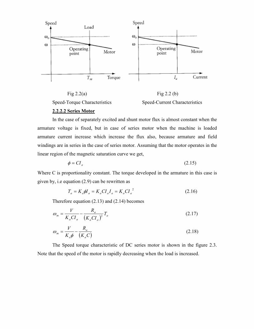
Fig 2.2(a) Fig 2.2 (b)
Speed-Torque Characteristics Speed-Current Characteristics
2.2.2.2 Series Motor
In the case of separately excited and shunt motor flux is almost constant when the
armature voltage is fixed, but in case of series motor when the machine is loaded
armature current increase which increase the flux also, because armature and field
windings are in series in the case of series motor. Assuming that the motor operates in the
linear region of the magnetic saturation curve we get,
(2.15) aCI=φ
Where C is proportionality constant. The torque developed in the armature in this case is
given by, i.e equation (2.9) can be rewritten as
(2.16) 2
aaaaaaaa CIKICIKIKT === φ
Therefore equation (2.13) and (2.14) becomes
( )(2.17)
2 a
aa
a
aa
m TCIK
R
CIK
V−=ω
( )(2.18)
CK
R
K
V
a
a
a
m −=φ
ω
The Speed torque characteristic of DC series motor is shown in the figure 2.3.
Note that the speed of the motor is rapidly decreasing when the load is increased.

Fig 2.3
Speed Torque Characteristic of DC series motor.
2.3 Conventional Methods of Speed Control of DC Motors
2.3.1 Speed control of separately excited or DC shunt motor
As seen from in the above section 2.2, the speed torque characteristic and speed current
characteristic of separately excited or shunt motor is as given below,
( )(2.19) -02
ωωφφ
ω ∆=−= a
a
a
a
m TK
R
K
V
( )(2.20) -0 ωω
φφω ∆=−=
a
aa
a
mK
IR
K
V
Where 0ω the no load is speed and ω∆ is the speed drop. The no load speed is computed
when the torque and current are equal to zero. The speed drop is a function of the load
torque. From the above expressions speed of the separately excited DC motor or Shunt
motor can be controlled by controlling the following quantities:
a) Resistance in the armature circuit: When the resistance is inserted in the
armature circuit, the speed drop ω∆ increases and the motor speed decreases.
b) Terminal Voltage (Armature voltage): Reducing the armature voltage V of the
motor reduces the motor speed.
c) Field Flux (or Field Voltage): Reducing Field voltage reduces the fluxφ , and
the motor speed increases.
Note: We cannot operate the electric motor with voltages higher than the rated value.
Therefore we cannot control the speed by increasing the armature or field voltages
beyond the rated values. Only voltage reduction can be implemented. Hence second
method of speed control is only suitable for speed reduction (armature voltage), where
third method (Field flux) is suitable for speed increase.

2.3.2 Controlling speed by adding external resistance to armature.
Figure 2.4 shows a DC motor setup with resistance added in the armature circuit.
Figure 2.5 shows the corresponding speed torque characteristics. Let us assume that the
load torque is unidirectional and constant. A good example for this type of torque is
elevator. Also assume that the field and armature voltages are constant.
Fig 2.4 Fig 2.5
A setup for speed change by adding Effect of adding an armature resistance
an armature resistance on speed
At point 1 no external resistance is added in the armature circuit. If a resistance
Radd1is added to the armature circuit, the motor operates at point 2, where the motor speed
2ω is
( )
(2.22)
(2.21)
20
1
2
202
12
ωωφφ
ω
ωωφφ
ω
∆−=+
−=
∆−=+
−=
a
a
adda
a
aadda
a
IK
RR
K
V
or
TK
RR
K
V
Note that the no load speed 0ω is unchanged regardless of the value of resistance
in the armature circuit. The second term of the speed equation is the speed droop ω∆ ,
which increase in magnitude when Radd increases. Consequently, the motor speed is
reduced. If the added resistance keeps increasing, the motor speed decreases until the
system operates at point 4, where the speed of the motor is zero. The operation of the
drive system at point 4 is known as “holding”.
Note: Operating a dc motor for a period of time with a resistance inserted in the
armature circuit is a very inefficient method. The use of resistance is acceptable only

when the heat produced by the resistance is utilized as a by product or when the
resistance is used for a very short period of time.
2.3.2 Controlling speed by adjusting armature voltage.
A common method of controlling speed is to adjust the armature voltage. This
method is highly efficient and stable and is simple to implement. The circuit of figure 2.6
shows the basic concept of this method.
Fig 2.6
A setup for speed change by adjusting armature voltage
The only controlled variable is the armature voltage of the motor, which is
represented as an adjustable voltage source. Based on equation 2.19, when armature
voltage is reduced no load speed is also reduced. Moreover for the same value of load
torque and field flux, the armature voltage does not affect the speed drop ω∆ . The slope
of speed torque characteristic is( )2φa
a
K
R, which is independent of the armature voltage.
Hence the characteristics are shown as figure 2.7. Note that it is assumed that the field
voltage is unchanged when the armature voltage varies.
Fig 2.7

2.3.2 Controlling speed by adjusting Field voltage
Equations (2.19) and (2.20) show the dependency of motor speed on the field
flux. The no load speed is inversely proportional to the flux and slope of equation (2.19)
is inversely proportional to square of the flux. Therefore the speed is more sensitive to
flux variations than to variations in the armature voltage.
Figure 2.8(a) shows a setup for controlling speed by adjusting the field flux. If we
reduce the field voltage, the field current and consequently the flux are reduced. Figure
2.8 (b) shows a set of speed torque characteristics for three values of field voltages. When
the field flux is reduced, the no load speed 0ω is increased in inverse proportion to the
flux, and the speed drop ω∆ is also increased.
Fig 2.8 (a) Fig 2.8(b)
The characteristics show that because of the change in speed drops, the lines are
not parallel. Unless the motor is excessively loaded, the motor speed increases when the
field is reduced. When motor speed is controlled by adjusting the field current, the
following considerations should be kept in mind:
a. The field voltage must not exceed the absolute maximum rating
b. Since DC motors are relatively sensitive to variations in field voltage, large
reductions in field current may result in excessive speed.
c. Because the armature current is inversely proportional to the field
flux
= φa
aa K
TI , reducing the field results in an increase in the armature
current (Assuming that the load torque is unchanged).
Thus by combining armature and field control for speeds below and above rated
speed, relatively a wide range of speed control is possible. For speeds lower than
that of the rated speed, applied armature voltage is varied while the field current is

kept at its rated value: to obtain speeds above the rated speed, field current is
decreased while keeping the applied armature voltage constant.
2.4 Controlled Rectifier Fed DC Drives
Controlled rectifiers are used to get variable dc voltage from an ac source of fixed
voltage. There are several types of converters which can be used for feeding DC motors.
AS thyristors are capable of conducting current in one direction all theses rectifiers are
capable of conducting current only in one direction.
2.4.1 Types of Rectifiers
AC to DC converters
(Or) Rectifiers
Single Phase type Three phase type
Uncontrolled Controlled
(Contains only DIODES) (Contains both SCR and Diodes)
Half Wave Full Wave
(1 Pulse) (2 Pulse)
Half wave full Half wave semi Full wave full Full wave semi
Converters without Converter with Converters without Converter with
Freewheeling Diode Freewheeling Diode FWD FWD
2.4.2 Single Phase rectifier fed separately Excited DC motor drive
The thyristor D.C. drive remains an important speed-controlled industrial
drive, especially where the higher maintenance cost associated with the D.C. motor
brushes is tolerable. The controlled (thyristor) rectifier provides a low-impedance
adjustable ‘D.C.’ voltage for the motor armature, thereby providing speed control. For
motors up to a few kilowatts the armature converter can be supplied from either single-
phase or three-phase mains, but for larger motors three-phase is always used. A separate
thyristor or diode rectifier is used to supply the field of the motor: the power is much less
than the armature power, so the supply is often single-phase. Figure 2.9 shows the setup
for single phase controlled rectifier fed separately excited dc motor drive. Field circuit is
also excited by a dc source, which is not shown in the figure just for simplicity.

Fig 2.9
The motor terminal voltage waveform and current waveform for the dominant
discontinuous and continuous conduction modes are shown in the figure 2.10(a) and 2.10
(b).Thyristors TA and TB are gated at αω =t .The SCR’s will get turned on only
if EVm >αsin . Thyristors TA and TB are given gate pulses from πα to and thyristors TA’
and TB’ are given gate pulses from ( ) παπ 2 to+ . When armature current does not flow
continuously the motor is said to operate in discontinuous conduction mode. When
current flows continuously, the conduction is said to be continuous. In discontinuous
modes, the current starts flowing with the turn on thyristors TA and TB at αω =t . Motor
gets connected to the source and its terminal voltage equals Vs.
At some angle β known as extinction angle, load current decays to zero.
Here πβ > . As TA and TB are reversed biased after πω =t , this pair is commutated at
βω =t when Ia=0. From ( )απβ + to , no SCR’s conducts, the terminal voltage jumps
from E tosin βmV .At βω =t as pair TA’ and TB
’ is triggered, load current starts to build
up again as before and load voltage Va follows Vs waveform as shown in the figure
2.10(a). At ( )βπ + , Ia falls to zero, Va changes from ( )βπ +sinmV to E as no SCR
conducts.

Fig 2.10 (a) Discontinuous Conduction Mode Waveforms
In continuous conduction mode, during the positive half cycle thyristiors TA and TB
are forward biased. At αω =t , TA and TB are turned ON. As a result, supply voltage
αsinmV immediately appears across thyristors TA’ and TB
’ as a reverse bias, they are
turned off by natural commutation. At ( )απω +=t forward biased SCR’s TA’ and TB
’
are triggered causing turn off of TA and TB.

Fig 2.10 (b) Continuous Conduction Waveforms
2.4.2.1Discontinuous Conduction:
The drive operates in two intervals.
a) Conduction period ( )βωα ≤≤ t , TA and TB conduct and V0=Vs.
Also ( ) ( )βπωαπ +≤≤+ t , TA’ and TB
’ conduct and V0=Vs.
b) Idle period ( )απωβ +≤≤ t when Ia=0 and Va=E.
Drive operation is described by the following equations

( )
(2.25) sin
dt
di
get we(2.23) From
(2.24) tfor 0i and
(2.23) tfor sin
a
a
a
ma
a
a
a
ma
aaaa
L
EtVi
L
R
EV
tVEdt
diLiRV
−==
+≤≤==
≤≤=++=
ω
απωβ
βωαω
In order to get the speed torque characteristics for different values of α of the controlled
rectifier fed separately excited DC motor, it is necessary to solve the above equation
(2.25). So solving the above equation involves two mathematical steps, one is to evaluate
the complementary solution of the equation (2.25) and particular integral solution of the
equation (2.25).
Solution to Complementary Function:
(2.26) 0
0dt
di
is (2.25)equation offunction ary complement The
a
=
+
=+
a
a
a
a
a
a
iL
R
dt
d
iL
R
(i.e.)The above equation is of the form 01 =
+ mdx
dwhere
dt
drepresents
dx
d and m1
representsa
a
L
R. Roots of the equation 01 =
+ mdx
dis D=-m1. Therefore the roots of the
equation 2.26 is m = -a
a
L
R. If the roots of the equation 01 =
+ mdx
d is real than the
complementary function is given by, C.F = mxeC1 therefore complementary function of
the equation (2.26) is given by,
C.F = (2.27) 1
t
aL
aR
eC
−
We know that for an RL circuit Z=R+jXL
a
a
a
a
a
a
L
R
L
R
R
L
=⇒
=⇒
=∴
φω
ωφ
ωφ
cot
cot
tan

Substituting the above relation in equation (2.27) we get,
C.F. = (2.28) cot
1φωt
eC−
Therefore the complementary function solution of the equation (2.25) is as given in
equation (2.28). The next step is to find the particular integral solution of equation (2.25).
In the expression (2.25) there are two Particular Integrals they are
P.I1=a
m
L
tV ωsin and the other one is P.I2=
aL
E−
Let us fine the solution of particular integrals one by one.
Solution to Particular Integral 1:
If X is sin (aX) or cos (aX) then the solution of P.I can be found out by
PI= aXDf
sin)(
1and replace D
2 by –a
2
Therefore P.I 1 can be written as,
tL
V
L
RD
PIa
m
a
a
ωsin1
1
+= Where D =
dt
dand a=ω
Multiplying and dividing by the conjugate in the above expression we get,
get, weexpression above in the D
sin
L
V
sin1
22
2
2a
m
ω
ω
ω
−=
−
−
=
−
+
−
=
replace
L
RD
tL
RD
tL
V
L
RD
L
RD
L
RD
PI
a
a
a
a
a
m
a
a
a
a
a
a

( ) (2.29) sincos
-
sin.cos
L
V
dt
dD since
sin.cos
L
V
sinsin
L
V
sin
1
222m
2
2222
a
m
2
222a
m
2
222a
m
2
2
2
+
−=
−−
−=
=
−−
−=
−−
−=
−−
−
=∴
aa
aa
a
aa
aa
a
aa
a
a
a
aa
a
a
a
a
a
a
a
m
RL
tRtLV
L
RL
tRLt
L
RL
tL
Rt
L
RL
tL
RtD
L
R
tL
RD
L
VPI
ωωωω
ωωωω
ω
ωωω
ω
ωω
ω
ω
Now let us consider a triangle as shown in the figure 2.11
Fig 2.11
From the above figure ( ) 22
cos
aa
a
RL
R
+=
ωφ and
( ) 22sin
aa
a
RL
L
+=
ω
ωφ
Substituting the above two relation in equation (2.29) we get
aR
( ) 22
aa RL +ω
φ
aLω

( ) ( ) ( )
[ ]
[ ]
( )[ ] (2.30) sin
cos.sinsin.cos
sin.coscos.sin
sincos222222
φω
ωφωφ
ωφωφ
ωω
ωω
ω
ω
−=
−=
−−=
+−
++−=
tZ
V
ttZ
V
ttZ
V
tRL
Rt
RL
L
RL
V
m
m
m
aa
a
aa
a
aa
m
Solution to Particular Integral 2:
(2.31)
LR
1
01
12
a
a
0
aa
i
a
a
a
a
a
a
R
E
L
E
DeL
E
L
RD
L
E
L
RD
PI
a
−=
−=
=
−
+
=
−
+
=
Q
So combining equations (2.28), (2.30) and (2.31) gives the solution of equation (2.25)
( )
( )
0t and 0)(icondition initial theusingby evaluated becan Cconstant
(2.34) tan
(2.33) R ZWhere
(2.32) sin)(
a1
1
22
a
cot
1
==
=
+=
+−−=
−
−
ωα
ωφ
ω
φωω φω
a
a
a
t
a
ma
R
L
L
eCR
Et
Z
Vti
( ) (2.35) sin cot
1
φαφα eR
E
Z
VC
a
m
−−−=
Substituting (2.35) in (2.32) we get,

( ) ( ) ( )
( )
( ) ( ) ( )
( ) ( )
[ ] ( ) [ ]
[ ]
[ ] [ ]
[ ]
[ ]( )
( )(2.41)
)(
coscosV
..coscos)(
V
coscosV
KK Where coscosV
(2.40)in (2.8) and (2.6) ngSubstituti
(2.40) coscosV
(2.39) and (2.38) equations From
(2.39) cossincoscosV
sin1
V
waveformsousdiscontinu From
(2.38) V
(2.37) ofsolution iterativeby evaluated becan
(2.37) sinsin)(i
(2.36) from 0i since
(2.36) sinsin
2
m
2
m
2
m
am
m
m
a
a
cot
a
a
cot
TK
R
K
RK
T
K
RK
T
K
KRK
T
ERI
dE
tdEtdtV
RIE
eR
E
Z
V
R
E
Z
V
eR
E
Z
V
R
Et
Z
Vi
a
m
am
am
ma
aa
m
aa
a
m
a
m
t
a
m
a
m
a
αβπ
αββα
ω
αβπ
βααβ
ω
βαππ
αβω
φπαβ
ωβαπ
παβ
βαπ
θθθπ
βαπβα
π
ωωωπ
β
φαφββ
β
φαφω
β
α
απ
β
φαβ
φαω
−−
−−
=
−−−
−=
−−=
−
=
−=−−
−=−−
=−+
+−=
+=
+=
−−−−−=
=
−−−−−=
∫
∫ ∫+
−−
−−
Q
For a givenα , there is a particular speed mcω when απβ += , indicating that at mcω , the
mode of operation changes from discontinuous to continuous. mcω is called as critical
speed. Substituting απβ += in equation (2.37) we get,
( ) ( ) ( )
( ) ( ) (2.43) 0sinsin
(2.42) sinsin
cotcot
cot
=+−−−−−
−−−−−+
−−
−+−
φπφπ
φααπ
φαφα
φαφαπ
eR
Ee
Z
V
R
E
Z
V
eR
E
Z
V
R
E
Z
V
a
m
a
m
a
m
a
m
( )[ ] [ ]
[ ] ( )[ ]
( )
( ) (2.45) 1
1sin
KE
(2.44) 1
1sin
1sin1
011sin
cot
cot
mc
cot
cot
cotcot
cotcot
−
+−=
=
−
+−=
+−=−
=−++−−
−
−
−
−
−−
−−
φπ
φπ
φπ
φπ
φπφπ
φπφπ
φαω
ω
φα
φα
φα
e
eV
KZ
R
e
eV
Z
RE
eZ
Ve
R
E
eR
Ee
Z
V
ma
mc
m
a
m
a
a
m
Continuous Conduction Mode
For continuous conduction, average output voltage is given by,
( )
(2.48) cos2
(2.47) cos2
V
(2.46) sin1
2M
a
TK
R
K
V
V
tdtVV
am
m
ma
−=
=
= ∫+
απ
ω
απ
ωωπ
απ
α
Fig 2.12
2.4.3 Three Phase Fully Controlled rectifier fed separately Excited DC motor drive
Three phase controlled rectifiers are used in large power DC motor drives. Three
phase controlled rectifier gives more number of voltage pulses per cycle of supply
frequency. This makes motor current continuous and filter requirement also less

The number of voltage pulses per cycle depends upon the number of thyristors
and their connections for three phase controlled rectifiers. In three phase drives,
the armature circuit is connected to the output of a three phase controlled rectifier.
Three phase drives are used for high power applications up to mega watts power
level. The ripple frequency of the armature voltage is higher than that of the
single phase drives and it requires less inductance in the armature circuit to reduce
the armature current ripple.
Three phase full converters are used in industrial applications up to 1500KW
drives. It is a two quadrant converter. i.e. the average output voltage is either
positive or negative but average output current is always positive.
2.4.3.1 Principle of Operation:
Three phase full converter bridge circuit connected across the armature terminals
is shown in the figure 2.13 and figure 2.14 shows the voltage and current waveforms
of the converter. The circuit works as a three phase AC to DC converter for firing
angle delay 00 900 <<α and as a line commutated inverter for 00 18090 <<α . A
three phase full converter fed DC motor is performed where regeneration of power is
required i.e. it performs two quadrant operation.
Figure 2.13
Basically, the controlled rectifier consists of six thyristors arranged in the form of
three legs with two series thyristors in each leg. The center points of three legs are
connected to a three-phase power supply. The transformer is not mandatory, but it

provides the advantages of voltage level change, electrical isolation, and phase shift from
the primary. In a three-phase bridge, one device in the positive group (Q1 Q3 Q5) and
another device from the negative group (Q4 Q6 Q2) must conduct simultaneously to
contribute load current id. Each thyristor is normally provided with pulse train firing for
the desired conduction interval. The speed of the motor can be controlled by firing angle
control of the thyristors.
Fig 2.14 Three-phase thyristor bridge waveforms in rectification mode (α = 40°)

Fig 2.15 Three-phase thyristor bridge waveforms inverting mode (α = 150°)
The average motor armature voltage is given by
( )
(2.51) cos33
V have We
(2.50) 6
sin3V substitute above In the
(2.49) )(3
a
ab
2
6
απ
ωπ
ω
ωπ
απ
απ
m
m
aba
V
tdtV
tdVV
=
+=
= ∫+
+
2.4.3.2 Speed Torque Relations:
The drive speed is given by
aaba RIEV += Where φωab KE =
Then aamaa RIKV += φω
(2.52) φ
ωa
aaa
mK
RIV −=
In separately excited DC motor TIK aa =φ therefore (2.52) becomes
( )(2.53) T
K
R-
2
a
a
φφω
a
a
mK
V=

Fig 2.16
2.5 Chopper Fed DC drives
A chopper is a static device that converts fixed DC input voltage to a variable dc
output voltage directly
A chopper is a high speed on/off semiconductor switch which connects source to
load and disconnects the load from source at a fast speed.
Choppers are used to get variable dc voltage from a dc source of fixed voltage.
Self commutated devices such as MOSFET’s, Power transistors, IGBT’s, GTO’s
and IGCT’s are used for building choppers because they can be commutated by a
low power control signal and do not need communication circuit and can be
operated at a higher frequency for the same rating.
Chopper circuits are used to control both separately excited and Series circuits.
2.5.1 Advantages of Chopper Circuits
Chopper circuits have several advantages over phase controlled converters
1. Ripple content in the output is small. Peak/average and rms/average current ratios
are small. This improves the commutation and decreases the harmonic heating of
the motor.

2. The chopper is supplied from a constant dc voltage using batteries. The problem
of power factor does not occur at all. The conventional phase control method
suffers from a poor power factor as the angle is delayed.
3. Current drawn by the chopper is smaller than in phase controlled converters.
4. Chopper circuit is simple and can be modified to provide regeneration and the
control is also simple.
2.5.2 Chopper Controlled Separately Excited DC motor
If the source of supply is D.C. (for example in a battery vehicle or a rapid transit
system) a chopper-type converter is usually employed. The chopper-fed motor is, if
anything, rather better than the phase-controlled, because the armature current ripple can
be less if a high chopping frequency is used.
2.5.2.1 Motoring Mode of Operation
A transistor is used to chop the DC input voltage in to pieces and chopped DC
voltage is given to the motor as shown in the figure 2.17. Current limit control is used in
chopper. In current limit control, the load current is allowed to vary between two given
limits (i.e. Upper and lower limits). The ON and OFF times of the transistor is adjusted
automatically, when the current increases beyond the upper limit the chopper is turned
off, the load current free wheels and starts to decrease. When the current falls below the
lower limit the chopper is turned ON. The current starts increasing if the load. The load
current and voltage waveforms are shown in the figure 2.18. By assuming proper limits
of current, the amplitude of ripple can be controlled.
Fig 2.17 Fig 2.18
The lower the current ripple, the higher the chopper frequency. By this switching
losses increase. Discontinuous conduction avoid in this case. The current limit control is
superior one.

Duty Interval
During the ON period of the chopper (i.e) duty interval 0 <t<tON, motor terminal voltage
Va is a source voltage V and armature current increases from ia1 to ia2. The operation is
describe by,
(2.54) tt0 ON≤≤=++ VEdt
diLIR aaaa
In this interval the armature current increases from Ia1 to Ia2 since the motor is connected
to the source during this interval, it is called as duty cycle.
Free Wheeling Interval
Chopper Tr is turned off at t=tON. Motor current free wheels through the diode D
and the motor terminal voltage is zero. During interval TttON ≤≤ . Motor operation
during this interval is known as free wheeling interval and is described by
(2.55) t t0 ON TEdt
diLIR aaaa ≤≤=++
During this interval current decreases from ia2 to ia1
Duty cycle (or) Duty Ratio:
Duty cycle is defined as the ratio of duty interval tON to chopper period T is called Duty
cycle (or) Duty Ratio.
(2.56)
T
t
PeriodChopper
IntervalDuty ON==δ
From figure 2.18
(2.57) 1
0
∫=ONt
a VdtT
V
Solving the above,
[ ]
(2.59) V
(2.58)
a
00
V
T
tV
T
Vdt
T
VV ON
tt
a tON
ON
δ=
=== ∫
Then the speed of the chopper drive can be obtained as
aaa RIEV +=
Substituting Va from equation (2.59) in the above equation we get,
(2.60) aaRIEV +=δ
Substituting mKE ω= we get

(2.61) a
m
aR
KVI
ωδ −=
From above equation we get
(2.62) K
RI
K
V aam −=
δω
Substituting aIKT φ= in above equation we get
(2.63) T2φ
δω
K
R
K
V a
m −=
The torque speed characteristics of chopper fed separately excited DC motor is shown in
the figure 2.19
Fig 2.19
2.5.2.2 Regenerative Braking Mode
Regenerative braking operation by chopper is shown in the figure 2.20. Regenerative
braking of a separately excited motor is fairly simple and can be carried out down to very
low speeds.
Fig 2.20 Fig 2.21
In regenerative mode, the energy of the load is fed back to the supply system. The
DC motor works as a generator during this mode. As long as the chopper is ON the

mechanical energy is converted in to electrical energy by the motor, now working as a
generator, increases the stored magnetic energy in the armature circuit. When chopper is
switched off, a large voltage appears across the motor terminals this voltage is more than
that of the supply voltage V and the energy stored in the inductance and energy supplied
by the machine is fed back to the supply system. When the voltage of the motor fall to V,
the diodes in the line blocks the current flow preventing any short circuit of the load can
be supplied to the source. Very effective braking of motor is possible up to extreme small
speeds.
Energy Storage Interval
The stored energy and energy supplied by the machine is fed to the source. The
interval 0 <t<tON is now called energy storage interval and interval TttON ≤≤ is the duty
interval.
Here duty ratio (2.64) T
tT ON−=δ
From figure 2.21
[ ] ( ) (2.65) t-TT
V
T
V
1ON
tt
ON
==== ∫ ∫T
T
t
T
t
a
ON ON
dtT
VVdt
TV
(2.66) 1
−=
−=
T
tV
T
tTVV ONON
a
Therefore the speed torque relations under braking operation is given as
( )(2.67) T
12φ
δω
K
R
K
V a
m −−
=
2.5.3 Chopper control of DC series motor 2.5.3.1 Motoring control of series motor
The main drawback in the analysis of a chopper controlled series motor arises due
to the non linear relationship between the induced voltage E and armature current Ia,
because of the saturation in the magnetization characteristic. At a given motor speed ,the
instantaneous back emf E changed between E1 and E2 as Ia changes between Ia1 and Ia2
as shown in figure 2.22

2.5.3.2 Regenerative Braking of DC series Motor
With chopper control, regenerative braking of series motor can also be obtained.
During regenerative braking, series motor functions as a self-excited series generator. For
self excitation current flowing through the winding (field) should assist residual
magnetism. Therefore when changing from motoring to braking connection, when
armature current reverses field current should flow in the same direction. This is achieved
by reversing the field with respect to armature when changing from motoring to braking
operation.
The speed of this drive mω can be derived from the following equation
a
aam
aamaa
aaa
K
RIV
RIVRIVE
VRIVE
+=
+=+=∴
=+=
δω
δωδ
δ
a
a
K
Vbut
The speed – torque characteristics gives unstable operation with most loads
shown in figure 2.23.Therefore regenerative braking of series motor is difficult.
2.5.4 Four Quadrant operation of DC Drive (or) TYPE – E Four Quadrant chopper
Fed Drive:Operation
The armature current Ia is either positive or negative (flow in to or away from
armature) the armature voltage Va is also either positive or negative. This is known as
four quadrant chopper drive. Two type – C choppers can be combined to form a class – E
chopper as shown in figure 2.24
First Quadrant – Forward motoring mode For first quadrant operation, thyristor S4 is kept on, thyristor S3 is kept off and thyristor
switch S1 is operated. With S1, S4 ON, armature voltage Va = Vs and armature control Ia
begins flow. Here both Va and Ia are positive giving first quadrant operation, when S1 is
turned off, positive current freewheels through S4, D2. In this manner, Va, Ia can be
controlled in this first quadrant, and operation gives forward motoring mode.
Second Quadrant – Forward braking mode
Here thyristor S2 is operated and S1 , S3 and S4 are kept off. With S4 on, reverse or
negative current flows through La, S2, D4 and Eb. During the operation time of S2, the
armature inductance ‘La’ stores energy during the time S2 is on. When S2 is turned off,
current is fed back to source through diodes D1 , D4 . Note that here ( E+L(di/dt)) is more
than the source voltage Vs .As the Vs is positive and Ia is negative, it is a second quadrant
operation gives forward braking mode. In that power is fed back from armature to source.
Third Quadrant – Reverse motoring mode For third quadrant operation, thyristor S1 is kept off, S2 is kept on and S3 is
operated, polarity of armature back emf Eb must be reversed for this quadrant operation.
With thyristor S3 is on, armature gets connected to source V. so that both Va , Ia are
negative, leading to third quadrant operation. When S3 is turned off,negative current free
wheels through S2,D4. In this manner only Va and Ia can be controlled in the third
quadrant.
Fourth Quadrant – Reverse Braking mode Here thyristor S4 is operated and other devices kept off, back emf Eb must have its
polarity reversed as in third quadrant operation. With S4 on, positive current flows
through S4,D2,La and Eb (armature). Armature inductance La stores energy during the time
S4 is on. When S4 is turned off, current is fed back to source through diodes D2, D3.Here
armature voltage Va is negative, but Ia is positive, leading to the chopper drive operation
in the fourth quadrant. Also power is fed back from armature to source. These four
quadrant operations are clearly depicted in figure 2.25.
Solved Problems
1. A 220 volts, 1500 rpm, 10 Amps separately excited dc motor has an armature
resistance of 10 Ω. It is fed from a single phase fully controlled bridge rectifier with
an ac source voltage of 230 volts, at 50 Hz. Assuming continuous load current,
compute
i. The motor speed at firing angle of 30 degrees and torque of 5 NM
ii. Developed torque at the firing angle of 45 degrees and speed of 1000 RPM

Solution:
V=200 Volts
N = 1500 rpm
Ia = 10 A
Ra= 10 Ω
Source Voltage Vs=230 volts
Under operating Conditions of separately excited DC motor
( )
diansSeconds/Ra Volts 7639.0
101060
1500 2220
KLet b
==
+
=
+=∴
=
+=
+=
ϕ
π
ω
ϕ
ϕω
bm
m
aamma
m
aamba
aaba
KK
xx
K
RIKV
K
RIKV
RIEV
i. For a torque of 5 Nm, motor armature current is
AK
TI
IKT
m
a
am
545.67639.0
5===
=
The equation giving the operation of converter motor is
230 V 50 Hz
-
+
Ia=10A
Ra=10Ω
F
FF
DC Supply

π
ω
ω
ωπ
ωαπ
ωαπ
απ
2
60 149.07 N RPMin SpeedMotor
sec/07.149
45.65 0.7639 179.33
10 545.6 7639.030cos230 2 2
cos230 2 2
cos2
cos2
m
x
rad
x
xxxx
RIKxx
RIKV
VRIEV
m
m
o
aamm
aammm
maaba
==
=
+=
+=
+=
+=
=+=
N= 1423.58 rpm
ii. For 045=α
( )
a
a
aammm
I
I
RIKV
1099.794.146
10 x 60
1000 x 2 x 7639.0cos
230 x 2 x 2
cos2
+=
+=
+=
πα
π
ωαπ
Ia=6.641 Amps
Motor developed torque
T = KmIa = 0.7639 x 6.641
T= 5.07 Nm
2. A separately excited DC motor rated at 10KW, 240 V, 1000 rpm is supplied from a
fully controlled two pulse bridge converter. The converter is supplied at 250 V, 50 Hz
supply. An extra inductance is connected in the load circuit to make the conduction
continuous. Determine the speed, power factor and efficiency of operation for thyristors
firing angles of 0 and 60 degrees assuming the armature resistance of 0.4 Ω and an
efficiency of 87% at rated conditions. Assume constant torque load
Solution:
The input current to the motor at rated conditions
Wxx 3
3
10494.1187.0
1010==
The supply current to the motor is

Ax
89.47240
10494.11 3
==
Neglecting the field copper loss the armature current = 47.89A
The back EMF at the rated conditions is
Voltsx 843.2204.089.47240 =−=
At 0=α , the converter voltage is
VoltsxxV
V ma 2250cos
25022cos
2 0 ===π
απ
As the load torque is constant the armature current is same. Therefore the back EMF is
Voltsx 844.2004.089.47225 =−=
We know that ωKEb =
sec/719.10460
21000rad
x==
πω
radVoltsE
K b sec/.11.2719.104
844.220===∴
ω
At 00=α
Speed = sec/235.95108.2
844.200rad
K
Eb ==
N= RPMx
43.9092
60235.95=
π
Displacement factor DF = 10cos 0 ==ϕCos
Power Factor PF = 9.00cos22
cos22 0 ==
πα
πxx
Input = 225 x 47.89 = 10775.25 W
Output varies linearly with speed
KWxoutput 094.91000
4.90910kw rpm 909.4at (rated) ==∴
%4.847752.10
094.9
/
/===∴
pi
POη
At 60=α , the converter voltage is
VoltsxxV
V m
a 5.11260cos25022
cos2 0 ===
πα
π
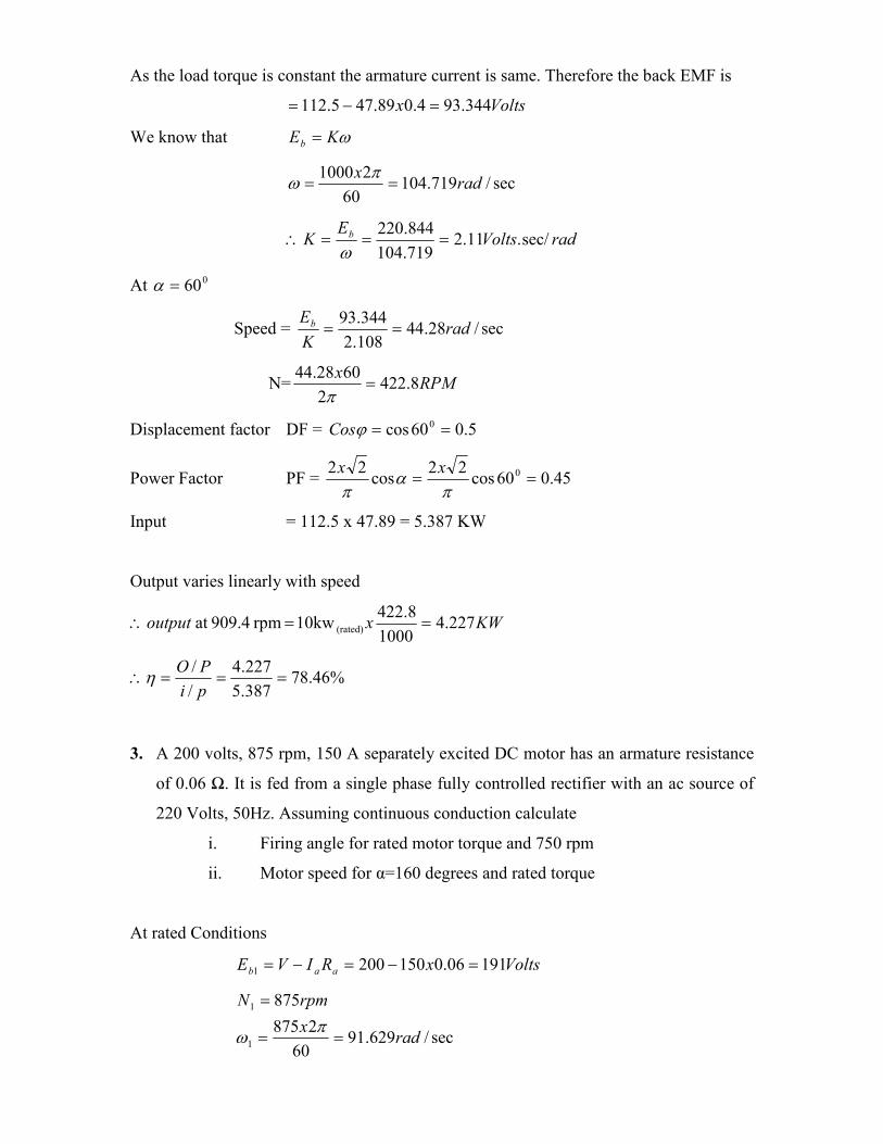
As the load torque is constant the armature current is same. Therefore the back EMF is
Voltsx 344.934.089.475.112 =−=
We know that ωKEb =
sec/719.10460
21000rad
x==
πω
radVoltsE
K b sec/.11.2719.104
844.220===∴
ω
At 060=α
Speed = sec/28.44108.2
344.93rad
K
Eb ==
N= RPMx
8.4222
6028.44=
π
Displacement factor DF = 5.060cos 0 ==ϕCos
Power Factor PF = 45.060cos22
cos22 0 ==
πα
πxx
Input = 112.5 x 47.89 = 5.387 KW
Output varies linearly with speed
KWxoutput 227.41000
8.42210kw rpm 909.4at (rated) ==∴
%46.78387.5
227.4
/
/===∴
pi
POη
3. A 200 volts, 875 rpm, 150 A separately excited DC motor has an armature resistance
of 0.06 Ω. It is fed from a single phase fully controlled rectifier with an ac source of
220 Volts, 50Hz. Assuming continuous conduction calculate
i. Firing angle for rated motor torque and 750 rpm
ii. Motor speed for α=160 degrees and rated torque
At rated Conditions
VoltsxRIVE aab 19106.01502001 =−=−=
sec/629.9160
2875
875
1
1
radx
rpmN
==
=
πω

We know that
radvoltsK
KEb
sec/.08.2629.91
191
11
==∴
= ω
I. 2bE at 750 rpm
voltsxE
radx
b 37.16354.7808.2
sec/54.7860
2750
2
2
==∴
==π
ω
( ) VoltsxRIEV aaba 7.17206.015037.1632 =+=+=∴
We know that
03.29
cos22022
7.172
cos2
=
=
=
α
απ
απ
xx
VV ma
II. At 0160=α N =? at rated torque
VoltsxxV
V m
a 12.186160cos22022
cos2 0 −===
πα
π
We know that aaba RIEV +=
( )
VoltsE
xE
b
b
12.195
06.015012.186
−=
+=−
rpmx
N 79.8952
6081.93
81.9308.2
12.195
−=−
=
−=−
=∴
π
ω
4. A 220 volts, 1500 rpm, 10 Amps separately excited dc motor has an armature
resistance of 0.5 Ω is fed from a three phase fully controlled rectifier. Available AC
source has a line voltage of 400 volts, 50 Hz. A star-delta connected transformer is
used to feed the armature so that motor terminal voltage equals rated voltage when
converter firing angle is zero. Calculate transformer turns ratio. Determine the value
of firing angle when
i. Motor is running at 1200 rpm and rated torque
ii. When motor is running at (-800 rpm) and twice the rated torque. Assume
continuous conduction

For 3 phase controlled rectifier the average output voltage is given by
απ
cos3 m
a
VV =
Given that Va =220 Volts
VoltsV
V
m
om
4.230
0cos3
220
=⇒
=∴π
At 1500 rpm
( ) voltsxRIVE aaab 2155.0102201 =−=−=
We know that
radvoltK
x
KEb
sec/.37.108.157
215
08.15760
215001
11
==
==
=∴
πω
ω
At 1200 rpm
VoltsxE
radvoltK
radx
KE
b
b
2.17266.12537.1
sec/.37.1
sec/66.12560
21200
2
2
22
==
=
==
=∴
πω
ω
Average output voltage is
( ) VoltsxRIEV aaba 1775.0102.1722 =+=+=
04.36
8.04.2303
177
3
3
=⇒
===⇒
=
α
ππα
απ
x
x
V
VCos
CosV
V
m
a
m
aQ
At -800 rpm, =α ? T = 2 x Irated
AxRatedCurrent
voltsxE
radx
b
202
77.11477.8337.1
sec/77.8360
2800
==
=−=∴
−=−
=π
ω
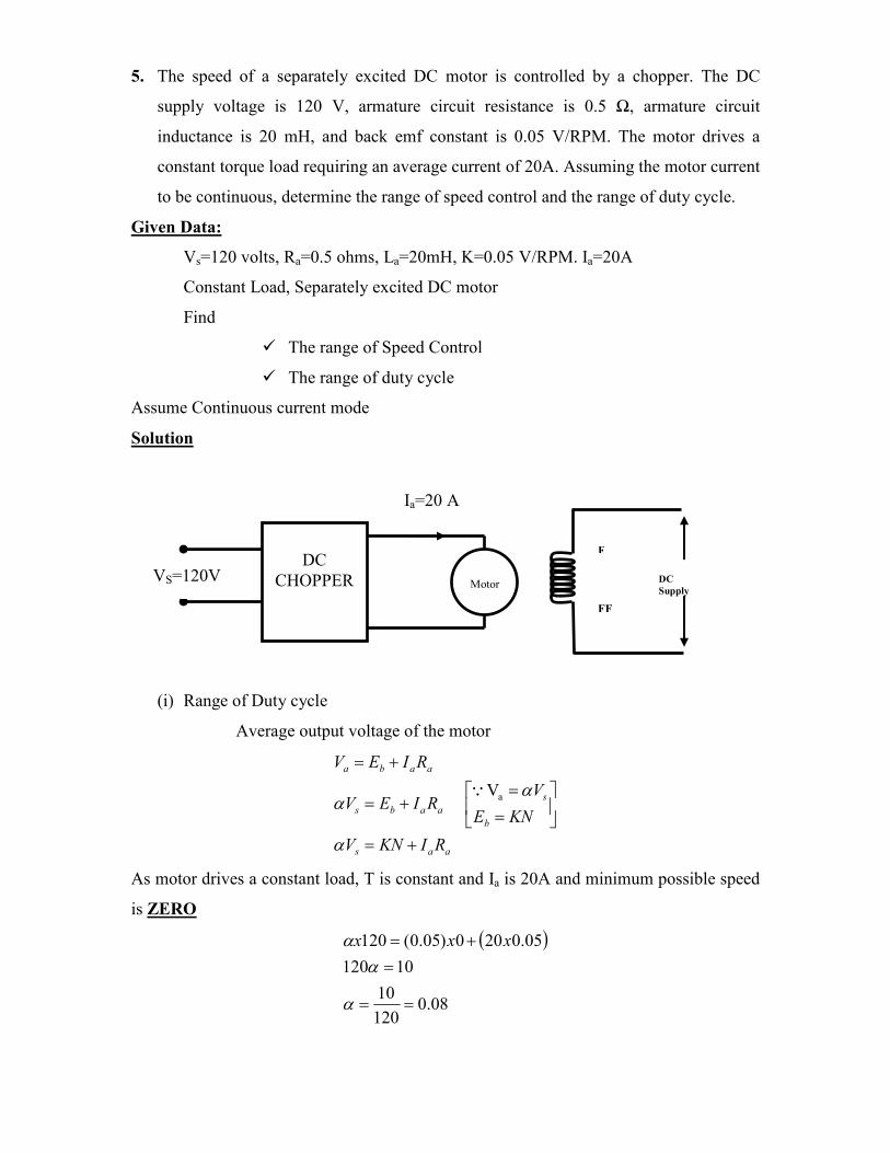
5. The speed of a separately excited DC motor is controlled by a chopper. The DC
supply voltage is 120 V, armature circuit resistance is 0.5 Ω, armature circuit
inductance is 20 mH, and back emf constant is 0.05 V/RPM. The motor drives a
constant torque load requiring an average current of 20A. Assuming the motor current
to be continuous, determine the range of speed control and the range of duty cycle.
Given Data:
Vs=120 volts, Ra=0.5 ohms, La=20mH, K=0.05 V/RPM. Ia=20A
Constant Load, Separately excited DC motor
Find
The range of Speed Control
The range of duty cycle
Assume Continuous current mode
Solution
(i) Range of Duty cycle
Average output voltage of the motor
aas
b
s
aabs
aaba
RIKNV
KNE
VRIEV
RIEV
+=
=
=+=
+=
α
αα aV
Q
As motor drives a constant load, T is constant and Ia is 20A and minimum possible speed
is ZERO
( )
08.0120
10
10120
05.0200)05.0(120
==
=
+=
α
αα xxx
DC
CHOPPER
Motor
F
FF
DC Supply
Ia=20 A
VS=120V
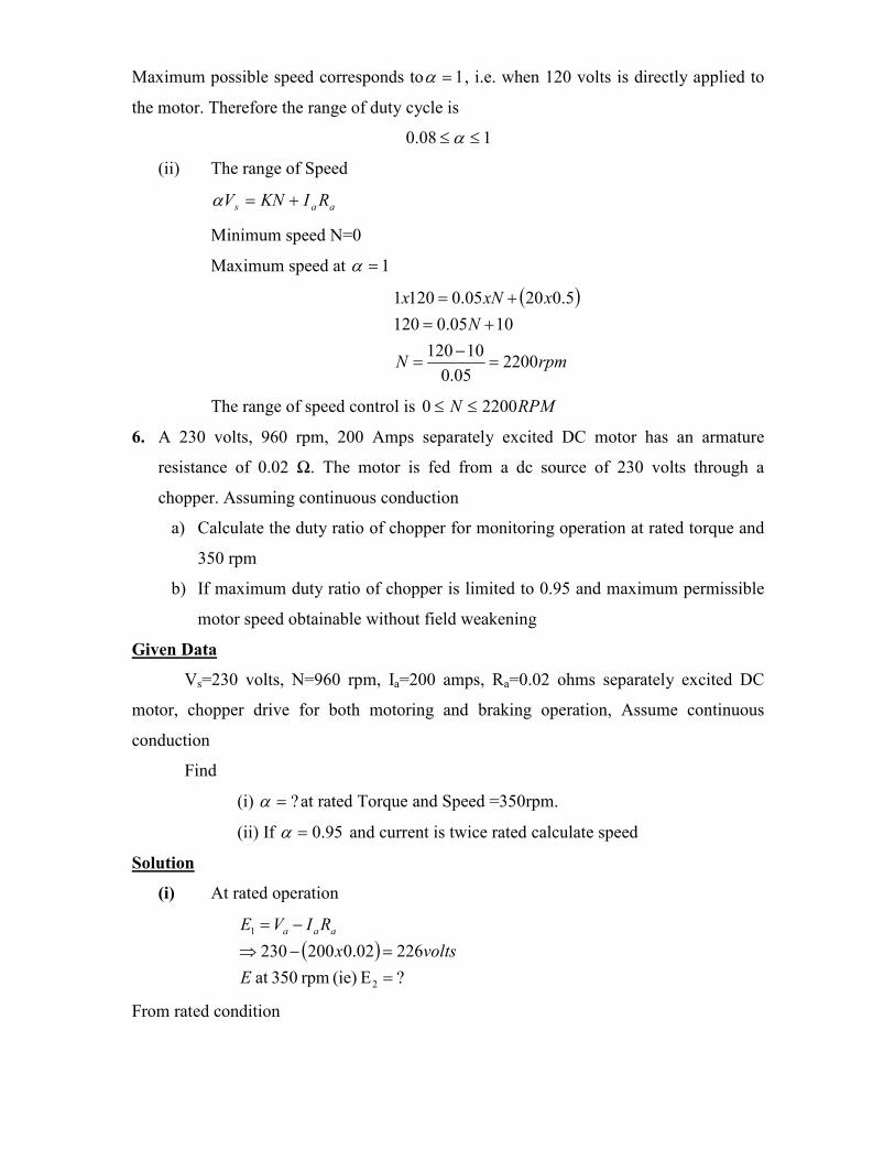
Maximum possible speed corresponds to 1=α , i.e. when 120 volts is directly applied to
the motor. Therefore the range of duty cycle is
108.0 ≤≤ α
(ii) The range of Speed
aas RIKNV +=α
Minimum speed N=0
Maximum speed at 1=α
( )
rpmN
N
xxNx
220005.0
10120
1005.0120
5.02005.01201
=−
=
+=
+=
The range of speed control is RPMN 22000 ≤≤
6. A 230 volts, 960 rpm, 200 Amps separately excited DC motor has an armature
resistance of 0.02 Ω. The motor is fed from a dc source of 230 volts through a
chopper. Assuming continuous conduction
a) Calculate the duty ratio of chopper for monitoring operation at rated torque and
350 rpm
b) If maximum duty ratio of chopper is limited to 0.95 and maximum permissible
motor speed obtainable without field weakening
Given Data
Vs=230 volts, N=960 rpm, Ia=200 amps, Ra=0.02 ohms separately excited DC
motor, chopper drive for both motoring and braking operation, Assume continuous
conduction
Find
(i) ?=α at rated Torque and Speed =350rpm.
(ii) If 95.0=α and current is twice rated calculate speed
Solution
(i) At rated operation
( )?E (ie) rpm 350at
22602.0200230
2
1
=
=−⇒
−=
E
voltsx
RIVE aaa
From rated condition

radVoltsK
radx
Kx
KE
sec/.24.253.100
226
sec/53.10060
2960
220
1
1
11
==∴
==
=
=
πω
ω
ω
2E at 350 rpm is given by
VoltsxE
x
1.8224.265.36
651.3660
2350
2
2
==∴
==π
ω
Motor terminal voltage at 350 rpm is
( )
37.0230
1.86
V
1.8602.02001.82
rpm 960
rpm 350
350
===
=+=
V
VoltsxV rpm
α
(ii) Maximum available
Volts 218.50.95x230 ==
= sa VV α
( ) VoltsxRIVE aaa 5.22202.02005.218 =+=+=∴
Speed at 222.5 volts Eb is
rpmx
N
rad
KEb
53.9482
60330.99
sec/330.9924.2
5.222
==
==
=
π
ω
ω
7. A DC series motor is fed from a 600 volts source through a chopper. The DC motor
has the following parameters armature resistance is equal to 0.04 Ω, field resistance is
equal to 0.06 Ω, constant 2-3 /10 x 4 AmpNmk = . The average armature current of 300
Amps is ripple free. For a chopper duty cycle of 60% determine
i. Input power drawn from the source.
ii. Motor speed and
iii. Motor torque.
Given Data
Vs=600 volts, Ia=300 amps, Ra=0.04 ohms, Rf=0.06 ohms, K= 23 /104 ampNmx − 6.0=δ
DC SERIES motor.

Solution
a. Power input to the motor = P = aa IV
KWxP
VoltsxVV sa
108300360
3606006.0
==∴
=== δ
b. For a DC series motor
[ ]
( ) ( )( )
M-N 360
3004x10
IKaT Torque
2626)sec(/5.272.1
30360
06.004.03003001046006.0
300104
KI
23-
2
a
3
3-
a
=
=
==
=−
=
++=⇒
++=++=∴
=
==
=
−
x
KIMotor
rpmorrad
xxxx
RRIKIRRIEV
xxx
I
KE
a
m
m
saamasaaa
m
am
maa
φ
ω
ω
ω
ω
φω
φω
Q
8. A 230 V, 1100 rpm, 220 Amps separately excited DC motor has an armature
resistance of 0.02 Ω. The motor is fed from a chopper, which provides both motoring
and braking operations. Calculate
i. The duty ratio of chopper for motoring operation at rated torque and 400 rpm
ii. The maximum permissible motor speed obtainable without field weakening, if
the maximum duty ratio of the chopper is limited to 0.9 and the maximum
permissible motor current is twice the rated current.
Given Data
Vs=230 volts, N=1100 rpm, Ia=220 amps, Ra=0.02 ohms separately excited DC
motor, chopper drive for both motoring and braking operation, Assume continuous
conduction
Find
(i) ?=α at rated Torque and Speed =400rpm.
(ii) If 9.0=α and current is twice rated calculate speed
Solution
(i) At rated operation

( )?E (ie) rpm 400at
6.22502.0220230
2
1
=
=−⇒
−=
E
voltsx
RIVE aaa
From rated condition
radVoltsK
radx
KE
sec/.95.1192.115
6.225
sec/192.11560
211101
11
==∴
==
=
πω
ω
2E at 400 rpm is given by
VoltsxE
radx
68.8195.1887.41
sec/887.4160
2400
2
2
==∴
==π
ω
Motor terminal voltage at 400 rpm is
( )
37.0230
1.86
V
1.8602.022068.81
rpm 1100
rpm 400
400
===
=+=
V
VoltsxV rpm
α
(ii) Maximum available
Volts 2070.9x230 ==
= sa VV α
( ) VoltsxxRIVE aaa 8.21502.02202207 =+=+=∴
Speed at 222.5 volts Eb is
rpmx
N
rad
KEb
78.10562
60667.110
sec/667.11095.1
8.215
==
==
=
π
ω
ω
9. A DC chopper is used to control the speed of a separately excited dc motor. The DC
voltage is 220 V, Ra= 0.2 Ω and motor constant Keφ =0.08 V/rpm. The motor drives a
constant load requiring an average armature current of 25 A. Determine
iv. The range of speed control
v. The range of duty cycle. Assume continuous conduction
Given Data:
Vs=220 volts, Ra=0.2 ohms, La=20mH, K=0.08 V/RPM. Ia=25A
Constant Load, Separately excited DC motor
Find
The range of Speed Control
The range of duty cycle
Assume Continuous current mode
Solution
(i) Range of Duty cycle
Average output voltage of the motor
aas
b
s
aabs
aaba
RIKNV
KNE
VRIEV
RIEV
+=
=
=+=
+=
α
αα aV
Q
As motor drives a constant load, T is constant and Ia is 25A and minimum possible speed
is ZERO
( )
04.0220
10
10220
2.0250)08.0(220
==
=
+=
α
αα xxx
Maximum possible speed corresponds to 1=α , i.e. when 120 volts is directly applied to
the motor. Therefore the range of duty cycle is
104.0 ≤≤α
(ii) The range of Speed
aas RIKNV +=α
Minimum speed N=0
Maximum speed at 1=α
( )
rpmN
N
xxNx
5.268708.0
5220
508.0220
2.02508.02201
=−
=
+=
+=
The range of speed control is RPMN 5.26870 ≤≤
Recommended