Eleventh Floor, Menzies Building Monash University, Wellington Road CLAYTON Vic 3800 AUSTRALIA
Telephone: from overseas: (03) 9905 2398, (03) 9905 5112 61 3 9905 2398 or 61 3 9905 5112
Fax: (03) 9905 2426 61 3 9905 2426 e-mail: [email protected]
Internet home page: http//www.monash.edu.au/policy/
Construction of a Database for a Dynamic
CGE Model for South Africa
by
LOUISE ROOS
Centre of Policy Studies Monash University
General Paper No. G-234 May 2013
ISSN 1 031 9034 ISBN 978 1 921654 42 8
The Centre of Policy Studies (COPS) is a research centre at Monash University devoted to economy-wide modelling of economic policy issues.

i
Construction of a database for a dynamic CGE model for South
Africa
Louise Roos
Centre of Policy Studies, Monash University, Australia, May 2013.
Abstract
This paper describes the construction of database constructed for a dynamic CGE model for
South Africa (hereafter SAGE). The starting point for creating a database for a CGE model
are official data from an Input/output (IO) table, or from a Supply Use Table (SUT), or from
a Social Accounting Matrix (SAM). Often the structure of the published data is not in the
required format of a CGE database, and so a major task is to transform the official data into
a form required by a CGE database. Four characteristics of the SAGE database are noted:
1. It contains information regarding the structure of the South African
economy in the base year (2002).
2. It is the initial solution to the SAGE model.
3. It has the same basic structure as the ORANIG and MONASH databases.
4. The basic database is supplemented by additional data relating to dynamics.
The database is organised in four parts. The first includes data on the coefficients that are
computed from the input–output (IO) table. These coefficients represent the basic flows of
commodities between users, commodity taxes paid by users, margin flows that facilitate the
flow of commodities and valued added matrices. The second part of the SAGE database
contains information on behavioural parameters. The elasticities influence the degree to
which economic agents change their behaviour when relative prices change. The third part
of the database contains information on government accounts, accounts with the rest of the
world and industry-specific capital stocks and depreciation rates. The fourth part of this
paper describes the tests undertaken to test for model validity.
This paper is set out as follows: Section 1 describes the structure of the IO database.
Section 2 reviews the official data sources used to create the IO database. Section 3
describes the steps taken to transform the official data into the correct format. Section 4
describes the elasticities and parameters adopted in for SAGE. Section 5 describes
additional information regarding industry-specific capital stocks and government accounts.
Section 6 describes various tests that were conducted to ensure that the database is
balanced. The paper ends with a conclusion.
Key words: Computable general equilibrium (CGE), Database, Africa, Supply Use Tables
JEL Code: C81, C68, O55

ii
iii
TABLE OF CONTENTS
LIST OF ABBREVIATIONS
LIST OF SETS
LIST OF TABLES
LIST OF FIGURES
1. Basic structure of a CGE database
1.1. Introduction…………………………………………………………………………………………….……1
1.2. Parameters………………………………………………………………………………………………….. 6
1.3. Data required for SAGE’s dynamic equations..……………………………….………………….… 6
2. Data sources…………………………………………………………………………………… 8
2.1. Note on the valuation of the tables………………………………………………….……… 8
2.2. Basic structure of the Supply-Use Tables (2002) for South Africa………………….. 8
2.2.1. The Supply table…………………………………………………………………. 9
2.2.2. The Use table……………………………………………………………………… 9
2.3. Other data sources……………………………………………………………………………... 10
2.3.1. Social accounting matrix (2002)……………………………………………… 10
2.3.2. South African Reserve Bank Quarterly Bulletin………………………….. 10
2.3.3. Government accounts…………………………………………………………... 11
2.3.4. Use of GTAP data to specify land rents……………………………………... 11
2.3.5. Sector-specific data………………………………………………………..……. 11
3. Stages in the compilation of the SAGE database…………………………………. 11
3.1. Step 1: Data mapping and aggregation………………………………………………….… 12
3.2. Step 2: Distribution of the residual………………………………………………………… 13
3.3. Step 3: Adjustments to the Supply and Use table………………………………………. 13
3.4. Step 4: Check that aggregate supply is equal to aggregate demand………………... 15
3.5. Step 5: Creating land rentals………………………………………………………………... 16
3.6. Step 6: Splitting flows into sources……………………………………………………….… 17
3.7. Step 7: Creating an Ownership of Dwellings commodity and industry…………….. 18
3.7.1. Value of output………………………………………………………………….….19
3.7.2. Sales structure………………………………………………………………….… 19
3.7.3. Input structure…………………………………………………………………… 19
3.8. Step 8: Creating margin matrices…………………………………………………………… 20
3.8.1. Calculation of aggregate margin matrices, by user………………………. 22
3.8.2. Creating margin matrices by type of margin commodity……………….. 22
3.9. Step 9: Creating tax matrices………………………………………………………………… 23
3.9.1. Defining the different taxes……………………………………………………. 23
3.9.2. Creating indirect tax matrices for all users……………………….……….. 25
3.9.3. Tax on production……………………………………………………………….. 26
3.10. Step 10: Creating matrices for the basic flows…………………………………………… 26
3.11. Step 11: Creating an industry dimension for the investor column………………….. 26
iv
3.11.1. Calculating industry-specific investment………..……………………………… 27
3.11.1.1. Calculating industry-specific depreciation rates d …….. 28
3.11.1.2. Calculating industry-specific capital growth rates k ….. 30
3.11.1.3. Calculating industry-specific rates of return R …………. 30
3.11.2. Completing the investment matrix………………………………………..…. 33
3.11.3. Determining industry-specific capital stocks……………………………....33
3.12. Step 12: Final balancing of the SAGE database……………………………………….… 34
3.12.1. Condition 1: industry cost should equal industry output…………….... 34
3.12.2. Condition 2: domestic commodity output equals domestic use…….… 34
4. Parameters and elasticities………..………………………………………………….… 36
4.1. The substitution parameters between primary factors…………………….………….. 37
4.2. The CES substitution elasticities between labour occupations……………………….38
4.3. The elasticities of substitution between domestic and foreign sources of supply.. 38
4.4. The constant elasticity of transformation (CET elasticity)………………………….… 40
4.5. Export demand elasticities………………………………………………………………..….. 40
4.6. The household expenditure and marginal budget shares………………………….…. 41
4.7. Frisch parameter……………………………………………………………………………….. 42
5. Additional data required for the dynamic equations……………………………. 43
5.1. Investment and capital stock…………………………………………………………….……43
5.1.1. Difference between maximum and trend growth rate of capital………. 43
5.1.2. Real interest rate…………………………………………………………………. 43
5.1.3. Asset price of capital…………………………………………………………..… 43
5.1.4. The average sensitivity of capital growth to changes in expected
rates of return…………………………………………………………………….. 43
5.1.5. CPI and lagged CPI………………………………………………………………. 43
5.2. Government accounts……………………………………………………………………….… 44
5.2.1. Revenue and expenditure items………………………………………………. 44
5.2.2. Tax rates on labour and capital incomes…………………………………… 45
5.2.3. Transfers…………………………………………………………………………… 46
5.2.4. Public sector debt and interest paid on public sector debt……………...46
5.2.5. Government investment………………………………………………………… 46
5.3. Accounts with the rest of the world………………………………………………………… 46
5.3.1. Gross national product (GNP)…………………………………………………. 47
5.3.2. Foreign debt and the interest rate on foreign debt in the base year…. 47
5.3.3. Exchange rate…………………………………………………………………….. 47
6. Test for model validity…………………………………………………………………….. 47
6.1. Test 1: Real and nominal homogeneity tests…………………………………………….. 47
6.2. Test 2: GDP from the income and expenditure side…………………………………….. 48
6.3. Test 3: Updated database should be balanced…………………………………………... 48
6.4. Test 4: Repeat the above steps using a multi-step solution method……………….. 48
6.5. Test 5: Explain the results……………………………………………………………………. 48
7. Concluding remarks………………………………………………………………………… 48

v
REFERNCES
Appendix 1. Elements in the sets modelled in SAGE……………………………………………………… 52
Appendix 2. Summary of parameters adopted in SAGE………………………………………………….. 54
vi
LIST OF ABBREVIATIONS
CAPM Capital Asset Pricing Model
CES Constant elasticity of substitution
CET Constant elasticity of transformation
CGE Computable General Equilibrium
IES Income and expenditure Survey
IMP Imports
IO Input-output
LFS Labour Force Survey
R Rand (South African currency)
RHS Right hand side
SAGE South African General Equilibrium model
SAM Social Accounting Matrix
SAQB South African Reserve Bank Quarterly Bulletin
SARB South African Reserve Bank
SIC Standard Industrial Classification of all economic activities
SNA System of National Accounts
StatsSA Statistics South Africa
SUT Supply-Use Tables
UN United Nations
vii
LIST OF SETS
COM Agricultural, Coal, Gold, Other mining, Food, Textiles, Petroleum,
Other non-metallic mineral products, Basic iron/steel, Electrical
machinery, Radio, Transport equipment, Other manufacturing,
Electricity, Water, Construction, Trade, Hotels and restaurants,
Transport services, Communications, Financial intermediation, Real
estate, Other business activities, General government, Health and
social work, Other activities, Owner Dwellings.
IND Agricultural, Coal, Gold, Other mining, Food, Textiles, Petroleum,
Other non-metallic mineral products, Basic iron/steel, Electrical
machinery, Radio, Transport equipment, Other manufacturing,
Electricity, Water, Construction, Trade, Hotels and restaurants,
Transport services, Communications, Financial intermediation, Real
estate, Other business activities, General government, Health and
social work, Other activities, Owner Dwellings.
MAR Trade, Transport services.
OCC Legislators, Professionals, Technicians, Clerks, Service workers,
Skilled agricultural workers, Craft workers, Plant and machine
operators, Elementary occupations, Domestic workers and
Occupations not else where specified.
SRC Domestic, Import.
viii
LIST OF TABLES
Table 1. Contents of the SAGE Input-Output data files……………………….….…5
Table 2. Contents of the additional data files…………………………………………. 7
Table 3. Different types of taxes (2002) (Rand millions)……………………….……. 24
Table 4. The values assigned to the risk index……………………………………..… 32
Table 5. Targets set for variables in the SAGE database…………………………… 36
Table 6. Consolidated account of the general government (2002)
(Rand millions)……………………………………………………………..………45
ix
LIST OF FIGURES
Figure 1. The SAGE input-output database……………………………….……………. 2
Figure 2. The format of the published Supply table………………………………….. 9
Figure 3. The format of the published Use table……………………………………… 10
Figure 4. Adjustment of purchases by residents abroad and non-residents
domestically………………………………………………………………………...14
Figure 5. Creating land rentals……………………………………………………………..16
Figure 6. Creating a source dimension: domestic and imports…………………..…17
Figure 7. Creating source dimensions for the margin matrices………………….… 22
Figure 8. Creating a source dimension for the tax matrices………………………... 25

1
1. BASIC STRUCTURE OF A CGE DATABASE
1.1 Introduction
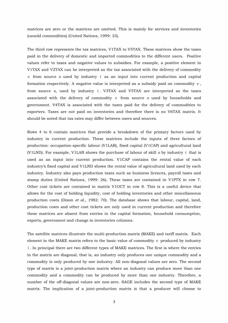
The SAGE model requires a database with separate matrices for basic, tax and margin flows
for both domestic and imported sources of commodities sold to domestic and foreign users,
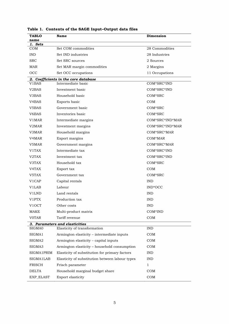
as well as matrices for the factors of production. The structure of the IO database is
illustrated in Figure 1 and the ingredients in the database are listed in Table 1. The first
three rows form the absorption matrix, rows 4 to 8 the production matrix and the two
satellite matrices are the multi-production matrix and the tariff matrix.
In the absorption matrix, users are identified in the column headings and denoted by a
number:
1. domestic producers divided into i industries;
2. investors divided into i industries;
3. a single representative household;
4. an aggregate foreign purchaser of exports;
5. government demand; and
6. changes in inventories.
The matrices in the first row, that is, V1BAS to V6BAS, represent direct flows of
commodities, from all sources to users valued at basic prices. The first matrix, V1BAS, can
be interpreted as the direct flow of commodity c , from source s , used by industry i as an
input into current production. V2BAS shows the direct flow of commodity c , from source s ,
used by industry i as an input to capital formation. V3BAS shows the flow of commodity c
from source s that is consumed by a representative household. V4BAS is a column vector
and shows the flow of commodity c to exports. V5BAS and V6BAS show the flow of
commodity c from source s to the government and change in inventories respectively. In
the IO database, no imported commodity is exported without being processed in a domestic
industry. Hence, V4BAS has no import dimension.
The matrices in row 1 contain only direct flows valued at basic prices. The basic price of a
domestic commodity is the price the producer receives, and excludes margin costs and sales
taxes. The basic price of an imported commodity is the duty-paid price, that is, the price at
the port of entry just after the commodity has cleared customs. It excludes all sales taxes
and margin costs but includes tariffs. It is assumed that the basic price is the same for all
users. The row sums are the total direct usage of a commodity. It should be noted that all
2
the values, with the exception of V6BAS, are positive. V6BAS records the change in
inventories, and thus can be positive or negative.
Figure 1. The SAGE input–output database
Absorption Matrix 1 2 3 4 5 6
Producers
Investors
Household
Export
Government
Change in Inventories
Size I I 1 1 1 1
1 Basic Flows
CS
V1BAS
V2BAS
V3BAS
V4BAS
V5BAS
V6BAS
2
Margins
CSM
V1MAR
V2MAR
V3MAR
V4MAR
V5MAR
n/a
3
Taxes
CS
V1TAX
V2TAX
V3TAX
V4TAX
V5TAX
n/a
4
Labour
OCC
V1LAB
C = Number of commodities
I = Number of industries
S = Sources (domestic, imported)
OCC = Number of occupation types
M = Number of commodities used as margins
5
Capital
1
V1CAP
6
Land
1
V1LND
7
Production Taxes
1
V1PTX
8 Other
Costs tickets
1
V1OCT
Joint production matrix
Tariffs
Size I Size 1
C
MAKE
C
V0TAR
The second row, V1MAR to V5MAR, represents the value of commodities used as margins to
facilitate the basic flows in row 1. SAGE includes two margin commodities, trade and
transport services. All margins are produced domestically. V1MAR and V2MAR are four-
dimensional matrices and show the cost of margin service m used to facilitate the flow of
commodity c , from source s to industry i . V3MAR and V5MAR are three dimensional and
show the cost of margin service m that facilitates the flow of commodity c from source s to
the representative household and the government respectively. V4MAR is a two-dimensional
matrix and shows the cost of margin service m that facilitates commodities flows to
exporters. There are flows that do not require any margins and therefore the values in these
Adapted from Horridge, 2006: 9.
3
matrices are zero or the matrices are omitted. This is mainly for services and inventories
(unsold commodities) (United Nations, 1999: 33).
The third row represents the tax matrices, V1TAX to V5TAX. These matrices show the taxes
paid in the delivery of domestic and imported commodities to the different users. Positive
values refer to taxes and negative values to subsidies. For example, a positive element in
V1TAX and V2TAX can be interpreted as the tax associated with the delivery of commodity
c from source s used by industry i as an input into current production and capital
formation respectively. A negative value is interpreted as a subsidy paid on commodity c ,
from source s, used by industry i . V3TAX and V5TAX are interpreted as the taxes
associated with the delivery of commodity c from source s used by households and
government. V4TAX is associated with the taxes paid for the delivery of commodities to
exporters. Taxes are not paid on inventories and therefore there is no V6TAX matrix. It
should be noted that tax rates may differ between users and sources.
Rows 4 to 6 contain matrices that provide a breakdown of the primary factors used by
industry in current production. These matrices include the inputs of three factors of
production: occupation-specific labour (V1LAB), fixed capital (V1CAP) and agricultural land
(V1LND). For example, V1LAB shows the purchase of labour of skill o by industry i that is
used as an input into current production. V1CAP contains the rental value of each
industry’s fixed capital and V1LND shows the rental value of agricultural land used by each
industry. Industry also pays production taxes such as business licences, payroll taxes and
stamp duties (United Nations, 1999: 26). These taxes are contained in V1PTX in row 7.
Other cost tickets are contained in matrix V1OCT in row 8. This is a useful device that
allows for the cost of holding liquidity, cost of holding inventories and other miscellaneous
production costs (Dixon et al., 1982: 70). The database shows that labour, capital, land,
production costs and other cost tickets are only used in current production and therefore
these matrices are absent from entries in the capital formation, household consumption,
exports, government and change in inventories columns.
The satellite matrices illustrate the multi-production matrix (MAKE) and tariff matrix. Each
element in the MAKE matrix refers to the basic value of commodity c produced by industry
i . In principal there are two different types of MAKE matrices. The first is where the entries
in the matrix are diagonal, that is, an industry only produces one unique commodity and a
commodity is only produced by one industry. All non-diagonal values are zero. The second
type of matrix is a joint-production matrix where an industry can produce more than one
commodity and a commodity can be produced by more than one industry. Therefore, a
number of the off-diagonal values are non-zero. SAGE includes the second type of MAKE
matrix. The implication of a joint-production matrix is that a producer will choose to
4
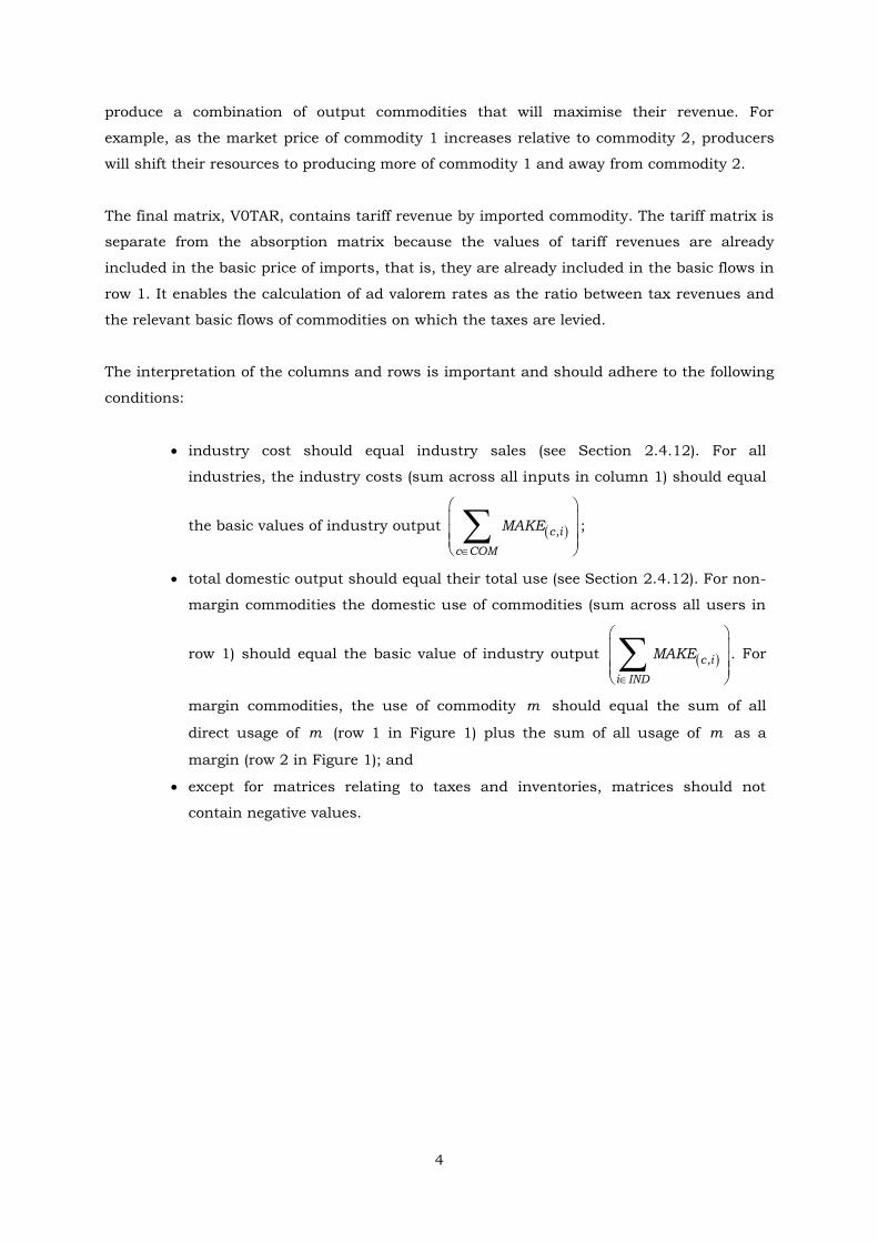
produce a combination of output commodities that will maximise their revenue. For
example, as the market price of commodity 1 increases relative to commodity 2, producers
will shift their resources to producing more of commodity 1 and away from commodity 2.
The final matrix, V0TAR, contains tariff revenue by imported commodity. The tariff matrix is
separate from the absorption matrix because the values of tariff revenues are already
included in the basic price of imports, that is, they are already included in the basic flows in
row 1. It enables the calculation of ad valorem rates as the ratio between tax revenues and
the relevant basic flows of commodities on which the taxes are levied.
The interpretation of the columns and rows is important and should adhere to the following
conditions:
industry cost should equal industry sales (see Section 2.4.12). For all
industries, the industry costs (sum across all inputs in column 1) should equal
the basic values of industry output
,c i
c COM
MAKE ;
total domestic output should equal their total use (see Section 2.4.12). For non-
margin commodities the domestic use of commodities (sum across all users in
row 1) should equal the basic value of industry output
,c i
i IND
MAKE . For
margin commodities, the use of commodity m should equal the sum of all
direct usage of m (row 1 in Figure 1) plus the sum of all usage of m as a
margin (row 2 in Figure 1); and
except for matrices relating to taxes and inventories, matrices should not
contain negative values.
5
Table 1. Contents of the SAGE Input–Output data files
TABLO name
Name Dimension
1. Sets
COM
IND
SRC
MAR
OCC
Set COM commodities
Set IND industries
Set SRC sources
Set MAR margin commodities
Set OCC occupations
28 Commodities
28 Industries
2 Sources
2 Margins
11 Occupations
2. Coefficients in the core database
V1BAS
V2BAS
V3BAS
V4BAS
V5BAS
V6BAS
V1MAR
V2MAR
V3MAR
V4MAR
V5MAR
V1TAX
V2TAX
V3TAX
V4TAX
V5TAX
V1CAP
V1LAB
V1LND
V1PTX
V1OCT
MAKE
V0TAR
Intermediate basic
Investment basic
Household basic
Exports basic
Government basic
Inventories basic
Intermediate margins
Investment margins
Household margins
Export margins
Government margins
Intermediate tax
Investment tax
Household tax
Export tax
Government tax
Capital rentals
Labour
Land rentals
Production tax
Other costs
Multi-product matrix
Tariff revenue
COM*SRC*IND
COM*SRC*IND
COM*SRC
COM
COM*SRC
COM*SRC
COM*SRC*IND*MAR
COM*SRC*IND*MAR
COM*SRC*MAR
COM*MAR
COM*SRC*MAR
COM*SRC*IND
COM*SRC*IND
COM*SRC
COM
COM*SRC
IND
IND*OCC
IND
IND
IND
COM*IND
COM
3. Parameters and elasticities
SIGMA0
SIGMA1
SIGMA2
SIGMA3
SIGMA1PRIM
SIGMA1LAB
FRISCH
DELTA
EXP_ELAST
Elasticity of transformation
Armington elasticity – intermediate inputs
Armington elasticity – capital inputs
Armington elasticity – household consumption
Elasticity of substitution for primary factors
Elasticity of substitution between labour types
Frisch parameter
Household marginal budget share
Export elasticity
IND
COM
COM
COM
IND
IND
1
COM
COM
6
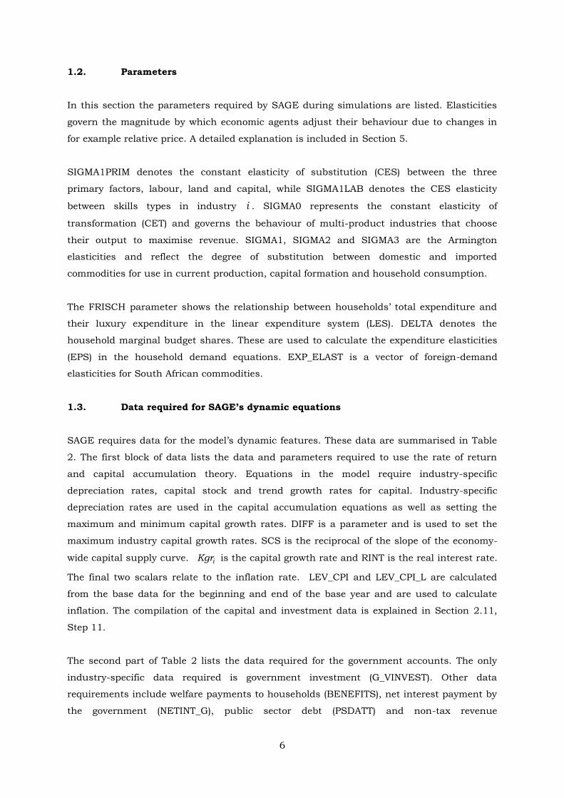
1.2. Parameters
In this section the parameters required by SAGE during simulations are listed. Elasticities
govern the magnitude by which economic agents adjust their behaviour due to changes in
for example relative price. A detailed explanation is included in Section 5.
SIGMA1PRIM denotes the constant elasticity of substitution (CES) between the three
primary factors, labour, land and capital, while SIGMA1LAB denotes the CES elasticity
between skills types in industry i . SIGMA0 represents the constant elasticity of
transformation (CET) and governs the behaviour of multi-product industries that choose
their output to maximise revenue. SIGMA1, SIGMA2 and SIGMA3 are the Armington
elasticities and reflect the degree of substitution between domestic and imported
commodities for use in current production, capital formation and household consumption.
The FRISCH parameter shows the relationship between households’ total expenditure and
their luxury expenditure in the linear expenditure system (LES). DELTA denotes the
household marginal budget shares. These are used to calculate the expenditure elasticities
(EPS) in the household demand equations. EXP_ELAST is a vector of foreign-demand
elasticities for South African commodities.
1.3. Data required for SAGE’s dynamic equations
SAGE requires data for the model’s dynamic features. These data are summarised in Table
2. The first block of data lists the data and parameters required to use the rate of return
and capital accumulation theory. Equations in the model require industry-specific
depreciation rates, capital stock and trend growth rates for capital. Industry-specific
depreciation rates are used in the capital accumulation equations as well as setting the
maximum and minimum capital growth rates. DIFF is a parameter and is used to set the
maximum industry capital growth rates. SCS is the reciprocal of the slope of the economy-
wide capital supply curve. iKgr is the capital growth rate and RINT is the real interest rate.
The final two scalars relate to the inflation rate. LEV_CPI and LEV_CPI_L are calculated
from the base data for the beginning and end of the base year and are used to calculate
inflation. The compilation of the capital and investment data is explained in Section 2.11,
Step 11.
The second part of Table 2 lists the data required for the government accounts. The only
industry-specific data required is government investment (G_VINVEST). Other data
requirements include welfare payments to households (BENEFITS), net interest payment by
the government (NETINT_G), public sector debt (PSDATT) and non-tax revenue
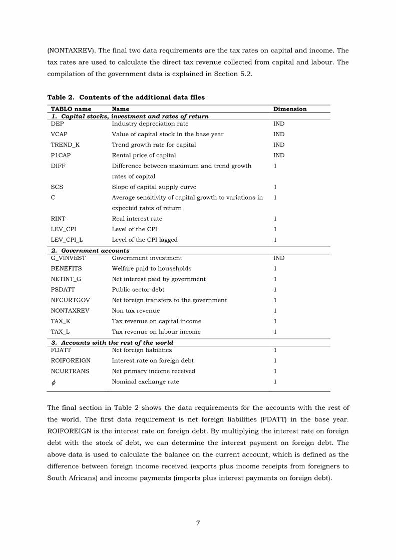
7
(NONTAXREV). The final two data requirements are the tax rates on capital and income. The
tax rates are used to calculate the direct tax revenue collected from capital and labour. The
compilation of the government data is explained in Section 5.2.
Table 2. Contents of the additional data files
TABLO name Name Dimension
1. Capital stocks, investment and rates of return
DEP
VCAP
TREND_K
P1CAP
DIFF
SCS
C
RINT
LEV_CPI
LEV_CPI_L
Industry depreciation rate
Value of capital stock in the base year
Trend growth rate for capital
Rental price of capital
Difference between maximum and trend growth
rates of capital
Slope of capital supply curve
Average sensitivity of capital growth to variations in
expected rates of return
Real interest rate
Level of the CPI
Level of the CPI lagged
IND
IND
IND
IND
1
1
1
1
1
1
2. Government accounts
G_VINVEST
BENEFITS
NETINT_G
PSDATT
NFCURTGOV
NONTAXREV
TAX_K
TAX_L
Government investment
Welfare paid to households
Net interest paid by government
Public sector debt
Net foreign transfers to the government
Non tax revenue
Tax revenue on capital income
Tax revenue on labour income
IND
1
1
1
1
1
1
1
3. Accounts with the rest of the world
FDATT
ROIFOREIGN
NCURTRANS
Net foreign liabilities
Interest rate on foreign debt
Net primary income received
Nominal exchange rate
1
1
1
1
The final section in Table 2 shows the data requirements for the accounts with the rest of
the world. The first data requirement is net foreign liabilities (FDATT) in the base year.
ROIFOREIGN is the interest rate on foreign debt. By multiplying the interest rate on foreign
debt with the stock of debt, we can determine the interest payment on foreign debt. The
above data is used to calculate the balance on the current account, which is defined as the
difference between foreign income received (exports plus income receipts from foreigners to
South Africans) and income payments (imports plus interest payments on foreign debt).
8
This concludes the description of the database requirements for the SAGE model. The
remainder of this chapter describes the data sources and the steps taken to create each of
the elements in the database.
2. DATA SOURCES
2.1. Note on the valuation of the tables
The 1993 System of National Accounts (SNA) recommends three ways in which production
(output) of goods and services can be measured (Statistics South Africa, 2006c: 12; United
Nations, 1999: 55). The definitions of these measures are given below.
Basic price: “The basic price is the amount receivable by the producer from the purchaser
for a unit of a good or service produced as output, minus any tax payable (i.e. VAT and
excise duties), and plus any subsidy receivable, on that unit as a consequence of its
production or sale. Basic prices exclude any transport charges involved separately by the
producer” (United Nations, 1999: 55).
Producers’ price: “The producers’ price is the amount receivable by the producer from the
purchaser for a unit of a good or service produced as output, minus VAT, or similar
deductible tax, invoiced to the producer. It excludes any transport charges invoiced
separately by the producer” (United Nations, 1999: 55).
Purchasers’ price: “The purchasers’ price is the amount paid by the producer, excluding any
deductible VAT or similar deductible tax, in order to take delivery of a unit of good and
service at the time and place required by the purchaser. The purchasers’ price includes any
transport charges paid separately by the purchaser to take delivery at the required time and
place” (United Nations, 1999: 55).
2.2. Basic structure of the Supply–Use tables for South Africa (2002)
The primary source of data is the Supply–Use tables (SUTs), published in 2002 by Statistics
South Africa (2006c).1 The Supply table (ST) contains information on the supply of
commodities from all sources whereas the Use table (UT) shows the final users of these
commodities.
1 A new set of Supply-Use table for 2005 are available. A number of the data manipulating step described in this
paper may be useful in creating the CGE database for 2005.
9
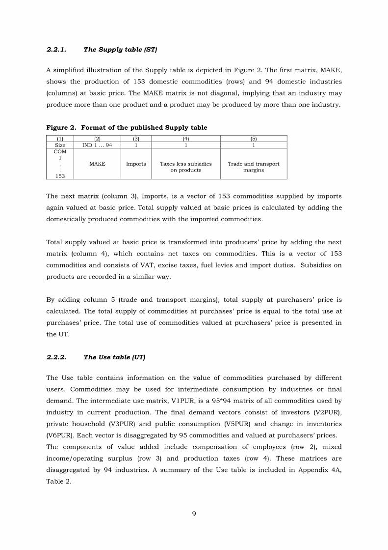
2.2.1. The Supply table (ST)
A simplified illustration of the Supply table is depicted in Figure 2. The first matrix, MAKE,
shows the production of 153 domestic commodities (rows) and 94 domestic industries
(columns) at basic price. The MAKE matrix is not diagonal, implying that an industry may
produce more than one product and a product may be produced by more than one industry.
Figure 2. Format of the published Supply table
(1) (2) (3) (4) (5)
Size IND 1 … 94 1 1 1
COM 1 .
. 153
MAKE
Imports
Taxes less subsidies
on products
Trade and transport
margins
The next matrix (column 3), Imports, is a vector of 153 commodities supplied by imports
again valued at basic price. Total supply valued at basic prices is calculated by adding the
domestically produced commodities with the imported commodities.
Total supply valued at basic price is transformed into producers’ price by adding the next
matrix (column 4), which contains net taxes on commodities. This is a vector of 153
commodities and consists of VAT, excise taxes, fuel levies and import duties. Subsidies on
products are recorded in a similar way.
By adding column 5 (trade and transport margins), total supply at purchasers’ price is
calculated. The total supply of commodities at purchases’ price is equal to the total use at
purchases’ price. The total use of commodities valued at purchasers’ price is presented in
the UT.
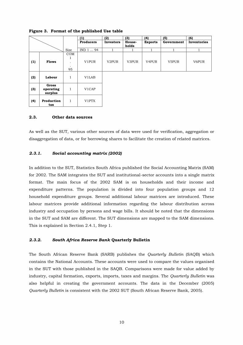
2.2.2. The Use table (UT)
The Use table contains information on the value of commodities purchased by different
users. Commodities may be used for intermediate consumption by industries or final
demand. The intermediate use matrix, V1PUR, is a 95*94 matrix of all commodities used by
industry in current production. The final demand vectors consist of investors (V2PUR),
private household (V3PUR) and public consumption (V5PUR) and change in inventories
(V6PUR). Each vector is disaggregated by 95 commodities and valued at purchasers’ prices.
The components of value added include compensation of employees (row 2), mixed
income/operating surplus (row 3) and production taxes (row 4). These matrices are
disaggregated by 94 industries. A summary of the Use table is included in Appendix 4A,
Table 2.
10
Figure 3. Format of the published Use table
(1) (2) (3) (4) (5) (6)
Producers Investors House-holds
Exports Government Inventories
Size IND 1 … 94 1 1 1 1 1
(1)
Flows
COM
1 . .
95
V1PUR
V2PUR
V3PUR
V4PUR
V5PUR
V6PUR
(2)
Labour
1
V1LAB
(3)
Gross operating surplus
1
V1CAP
(4)
Production
tax
1
V1PTX
2.3. Other data sources
As well as the SUT, various other sources of data were used for verification, aggregation or
disaggregation of data, or for borrowing shares to facilitate the creation of related matrices.
2.3.1. Social accounting matrix (2002)
In addition to the SUT, Statistics South Africa published the Social Accounting Matrix (SAM)
for 2002. The SAM integrates the SUT and institutional-sector accounts into a single matrix
format. The main focus of the 2002 SAM is on households and their income and
expenditure patterns. The population is divided into four population groups and 12
household expenditure groups. Several additional labour matrices are introduced. These
labour matrices provide additional information regarding the labour distribution across
industry and occupation by persons and wage bills. It should be noted that the dimensions
in the SUT and SAM are different. The SUT dimensions are mapped to the SAM dimensions.
This is explained in Section 2.4.1, Step 1.
2.3.2. South Africa Reserve Bank Quarterly Bulletin
The South African Reserve Bank (SARB) publishes the Quarterly Bulletin (SAQB) which
contains the National Accounts. These accounts were used to compare the values organised
in the SUT with those published in the SAQB. Comparisons were made for value added by
industry, capital formation, exports, imports, taxes and margins. The Quarterly Bulletin was
also helpful in creating the government accounts. The data in the December (2005)
Quarterly Bulletin is consistent with the 2002 SUT (South African Reserve Bank, 2005).
11
2.3.3. Government accounts
It was very difficult to find consistent government data. Treasury, Statistics South Africa
and the Reserve Bank publish government data, but the data are not consistent, which
makes comparison very difficult. The December 2005 Quarterly Bulletin contains
information on government accounts which is broadly consistent with the government
information in the SUT. The information in the SAQB is used to create the government
accounts.
2.3.4. Use of GTAP data to specify land rents
The GTAP 6.0 database (Dimaranan, 2006) includes an extra factor of production, namely
land. None of the above data sources explicitly provides data on land and therefore the
GTAP database for South Africa is used to create land rentals for the agricultural and
mining industries.
2.3.5. Sector-specific data
In the SUT and SAM, gross fixed capital-formation data is given as a vector. This vector
shows which commodities are used for investment by a single aggregate investor. However,
SAGE requires capital formation to be disaggregated by industry. Hence, industry-specific
information is required so that the single investment column can be split into 28 industry
columns. The Annual Financial Statistics Survey is used to obtain such industry-specific
data (Statistics South Africa, 2006a).
3. STAGES IN THE CONSTRUCTION OF THE SAGE DATABASE
The core database required by SAGE is described in Section 1 and Figure 1. The final SAGE
database, which fits this form, includes 28 commodities, 28 industries, 11 occupational
groups, two margin commodities and two sources. The elements of the different dimensions
(sets) are listed in Appendix 1. Although the SUT conforms to the international statistical
standards for the measurement of an economy as set out in the 1993 System of National
Accounts (SNA), it is not in the correct format needed for the SAGE database. Several steps
were taken to convert the published data into the required format. These steps are
discussed in this section.
To promote transparency and to facilitate auditing, the process of converting the published
data into the SAGE database was automated by writing a sequence of procedures coded in
GEMPACK (Harrison & Pearson, 1996, 2002; Pearson, 2002). Each step in the data
12
manipulation process addresses a specific data query and the output of a step is used as an
input in the next step. The process is as follows (Horridge, 2006):
Data are converted from their original hard copy or Excel format into Header
Array files;
Each data manipulation process is programmed in a TABLO file. The TABLO
file includes all the data manipulation equations, written in TABLO code, and
uses the VIEWHAR files as input files; and
To make sure that the balancing requirements are not violated test or check
commands are included in each step.
This automated process has a number of advantages. Firstly, each TABLO file serves as a
record of the process used to manipulate the data. Secondly, adjustments and corrections to
formulas can easily be made. Thirdly, the automation enables fast replications of the
process when needed. This is very useful when new data becomes available. Finally,
recording each step promotes transparency and avoids any “black box” issues, that is, the
data programs become a permanent documentation of the data manipulation process. The
next section describes the steps taken to convert the published data into the required IO
database.
3.1. Step 1: Data mapping and aggregation
The dimensions of the SAGE database differ from those of the published data. SAGE
includes an aggregated database with the dimensions of 28 commodities, 28 industries, 11
occupational groups, two margin commodities and two sources. There are several reasons to
support a smaller, aggregated database. Firstly, the aggregated database ensures improved
management of data. Secondly, most of the secondary data used to verify or compare data,
are published either on a macro level or on a highly aggregated level. Thirdly, when it is
necessary to disaggregate a commodity or industry, it is easier to adapt shares from other
sources. Finally, it is not necessary to include a highly disaggregated database. The focus of
this thesis is on the effects of HIV/AIDS on the labour market with specific emphasis on
labour supply. The emphasis is to ensure that (1) the linkages between SAGE and the health
extension are correct and (2) that the dynamic features are operational. If required, the core
database can be disaggregated.
The commodities and industries, as they appear in the SUT, are mapped to 272 commodities
and industries by using the Standard Industrial Classification of all Economic Activities
(SIC) (Statistics South Africa). The GEMPACK program, VIEWHAR, was used to turn
2 The final database includes 28 commodities and 28 industries. The additional commodity and industry (Owner
dwelling) is created in Step 7.
13
spreadsheet data into entries in a single HAR file called FID.HAR. An additional file,
SETINFO, is also created where all the set information is organised. This file remains the
same in all steps.
Firstly, the 153 commodities are mapped to 27 commodities and the 94 industries are
mapped to 27 industries (Statistics South Africa, 2006c: 46). The mapping of commodities
and industries is useful in identifying any misprints and irregularities that may be present
in the data. Since, in this step, no data adjustment has occurred and in the absence of any
irregularities, the mapped data should correspond to the published SAM data. No misprints
or irregularities were noted.
3.2. Step 2: Distribution of the residual
The output files of Step 1, FID.HAR and SETINFO.HAR, are used as input files in Step 2. The
Use tables include a commodity-specific residual. This residual is included because GDP
calculated according to the production and income approach, differs from GDP calculated
from the expenditure side. Firstly, the production and generation of income accounts are
compiled for each industry. These accounts are consistent with both the production and
income approach. GDP is therefore calculated from the supply side and then transferred to
the demand side (Use table). Secondly, the values for the components of final demand, as
they appear in the Use table, are then adjusted to be consistent with the values published
by the South African Reserve Bank (SARB). The SARB calculates GDP using the expenditure
approach. Their estimations allow for the compilation of the goods and services account in
which the residual item can be calculated.
In the 2002 SUT the residual item is negligible and therefore allocated to the “change in
inventories” vector. This ensures that commodity-specific aggregated supply is equal to
commodity-specific aggregate demand with only the “change to inventory” vector changed.
3.3. Step 3: Adjustments to the Supply and Use table
Several adjustments are included in the SUT published by Statistics South Africa. The first
adjustment relates to “purchases by residents abroad” and the second to “purchases by
non-residents in South Africa”. “Purchases by residents abroad” affect both the import
column and the household expenditure column. This adjustment is accounted for by adding
a positive value to both these columns. There is no detailed information regarding
commodity-specific purchases by residents abroad; only one value is given in the Use table
(R19,601 million).
14
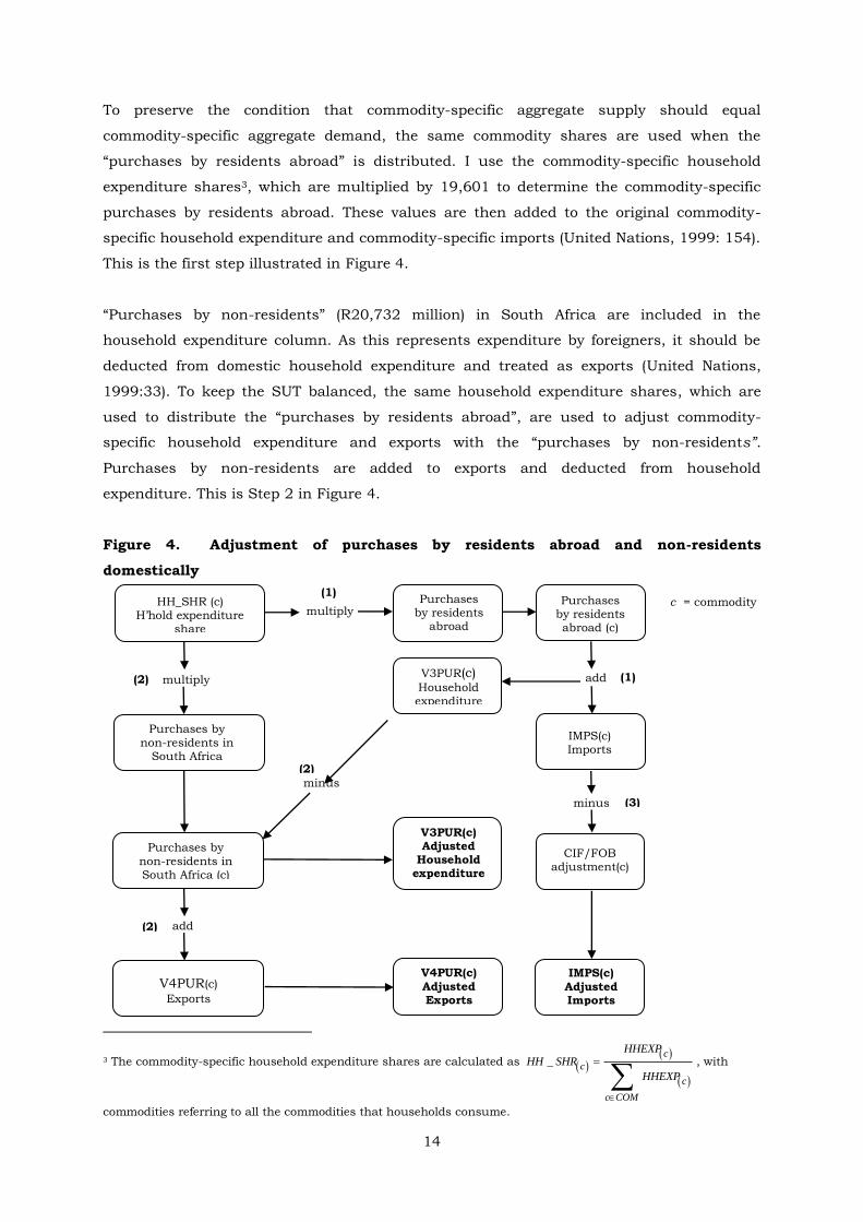
To preserve the condition that commodity-specific aggregate supply should equal
commodity-specific aggregate demand, the same commodity shares are used when the
“purchases by residents abroad” is distributed. I use the commodity-specific household
expenditure shares3, which are multiplied by 19,601 to determine the commodity-specific
purchases by residents abroad. These values are then added to the original commodity-
specific household expenditure and commodity-specific imports (United Nations, 1999: 154).
This is the first step illustrated in Figure 4.
“Purchases by non-residents” (R20,732 million) in South Africa are included in the
household expenditure column. As this represents expenditure by foreigners, it should be
deducted from domestic household expenditure and treated as exports (United Nations,
1999:33). To keep the SUT balanced, the same household expenditure shares, which are
used to distribute the “purchases by residents abroad”, are used to adjust commodity-
specific household expenditure and exports with the “purchases by non-residents”.
Purchases by non-residents are added to exports and deducted from household
expenditure. This is Step 2 in Figure 4.
Figure 4. Adjustment of purchases by residents abroad and non-residents
domestically
3 The commodity-specific household expenditure shares are calculated as
_
c
c
c
c COM
HHEXPHH SHR
HHEXP
, with
commodities referring to all the commodities that households consume.
c = commodity HH_SHR (c) H’hold expenditure
share
Purchases by residents abroad (c)
add
add
(2)
(3)
minus
minus
(2)
(1)
(2)
multiply
multiply
(1)
Purchases by
non-residents in South Africa
Purchases by residents
abroad
V3PUR(c) Household expenditure
IMPS(c) Imports
CIF/FOB adjustment(c)
Purchases by
non-residents in South Africa (c)
V4PUR(c)
Exports
V3PUR(c) Adjusted
Household expenditure
V4PUR(c)
Adjusted Exports
IMPS(c)
Adjusted Imports
15
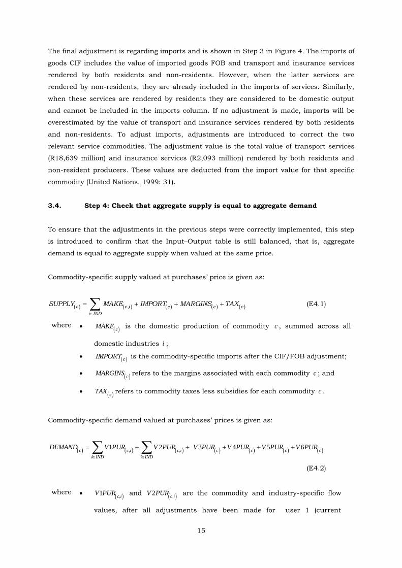
The final adjustment is regarding imports and is shown in Step 3 in Figure 4. The imports of
goods CIF includes the value of imported goods FOB and transport and insurance services
rendered by both residents and non-residents. However, when the latter services are
rendered by non-residents, they are already included in the imports of services. Similarly,
when these services are rendered by residents they are considered to be domestic output
and cannot be included in the imports column. If no adjustment is made, imports will be
overestimated by the value of transport and insurance services rendered by both residents
and non-residents. To adjust imports, adjustments are introduced to correct the two
relevant service commodities. The adjustment value is the total value of transport services
(R18,639 million) and insurance services (R2,093 million) rendered by both residents and
non-resident producers. These values are deducted from the import value for that specific
commodity (United Nations, 1999: 31).
3.4. Step 4: Check that aggregate supply is equal to aggregate demand
To ensure that the adjustments in the previous steps were correctly implemented, this step
is introduced to confirm that the Input–Output table is still balanced, that is, aggregate
demand is equal to aggregate supply when valued at the same price.
Commodity-specific supply valued at purchases’ price is given as:
,c c i c c c
i IND
SUPPLY MAKE IMPORT MARGINS TAX
(E4.1)
where cMAKE is the domestic production of commodity c , summed across all
domestic industries i ;
cIMPORT is the commodity-specific imports after the CIF/FOB adjustment;
cMARGINS refers to the margins associated with each commodity c ; and
cTAX refers to commodity taxes less subsidies for each commodity c .
Commodity-specific demand valued at purchases’ prices is given as:
1 2 3 4 5 6
c c i c i c c c c
i IND i IND
DEMAND V PUR V PUR V PUR V PUR V PUR V PUR, ,
(E4.2)
where 1c i
V PUR,
and 2c i
V PUR,
are the commodity and industry-specific flow
values, after all adjustments have been made for user 1 (current
16
production) and user 2 (investors). These flows are summed across
industries;
3c
V PUR is the commodity-specific flow values, after all adjustments have
been made for user 3 (households);
4c
V PUR is commodity-specific flow values for user 4 (exports);
5c
V PUR is commodity-specific flow values for user 5 (government); and
6c
V PUR is commodity-specific flow values for user 6 (inventories).
This check confirms that the adjustment had been performed correctly.
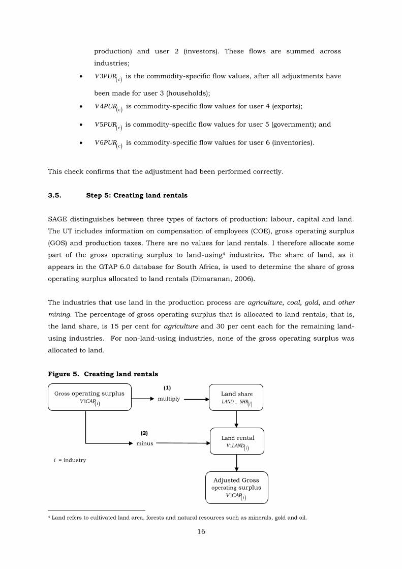
3.5. Step 5: Creating land rentals
SAGE distinguishes between three types of factors of production: labour, capital and land.
The UT includes information on compensation of employees (COE), gross operating surplus
(GOS) and production taxes. There are no values for land rentals. I therefore allocate some
part of the gross operating surplus to land-using4 industries. The share of land, as it
appears in the GTAP 6.0 database for South Africa, is used to determine the share of gross
operating surplus allocated to land rentals (Dimaranan, 2006).
The industries that use land in the production process are agriculture, coal, gold, and other
mining. The percentage of gross operating surplus that is allocated to land rentals, that is,
the land share, is 15 per cent for agriculture and 30 per cent each for the remaining land-
using industries. For non-land-using industries, none of the gross operating surplus was
allocated to land.
Figure 5. Creating land rentals
4 Land refers to cultivated land area, forests and natural resources such as minerals, gold and oil.
i = industry
Land share
iLAND SHR_ multiply
Adjusted Gross
operating surplus
1i
V CAP
Gross operating surplus
1i
V CAP
minus
(1)
(2) Land rental
1i
V LAND
17
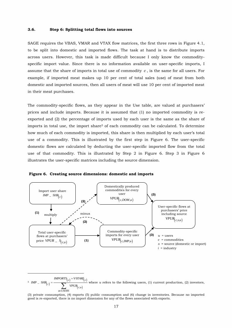
3.6. Step 6: Splitting total flows into sources
SAGE requires the VBAS, VMAR and VTAX flow matrices, the first three rows in Figure 4.1,
to be split into domestic and imported flows. The task at hand is to distribute imports
across users. However, this task is made difficult because I only know the commodity-
specific import value. Since there is no information available on user-specific imports, I
assume that the share of imports in total use of commodity c , is the same for all users. For
example, if imported meat makes up 10 per cent of total sales (use) of meat from both
domestic and imported sources, then all users of meat will use 10 per cent of imported meat
in their meat purchases.
The commodity-specific flows, as they appear in the Use table, are valued at purchasers’
prices and include imports. Because it is assumed that (1) no imported commodity is re-
exported and (2) the percentage of imports used by each user is the same as the share of
imports in total use, the import share5 of each commodity can be calculated. To determine
how much of each commodity is imported, this share is then multiplied by each user’s total
use of a commodity. This is illustrated by the first step in Figure 6. The user-specific
domestic flows are calculated by deducting the user-specific imported flow from the total
use of that commodity. This is illustrated by Step 2 in Figure 6. Step 3 in Figure 6
illustrates the user-specific matrices including the source dimension.
Figure 6. Creating source dimensions: domestic and imports
5
0
,
_c c
c
c u
u USERS
IMPORTS V TARf
IMP SHRVPUR
where u refers to the following users, (1) current production, (2) investors,
(3) private consumption, (4) exports (5) public consumption and (6) change in inventories. Because no imported
good is re-exported, there is no import dimension for any of the flows associated with exports.
(1) minus
u = users
c = commodities
s = source (domestic or import)
i = industry
(1)
(2)
(3)
(3)
Total user-specific flows at purchasers’
price c uVPUR S ,_
Import user share
IMP SHRc
_
User-specific flows at
purchasers’ price including source
c s uVPUR , ,
multiply
Commodity-specific imports for every user
c IMP uVPUR , ,
Domestically produced commodities for every
user
c DOM uVPUR , ,
(2)

18
3.7. Step 7: Creating an “Ownership of Dwellings” commodity and industry
In the original SUT there was no explicit recognition of the imputed value of owner-occupied
dwellings (OwnerDwel). Ownership of dwellings is an important component of household
expenditure as it is closely linked to household income and as such can give additional
insight into the economic wellbeing of the population. In a dynamic setting, we would also
expect that as per capita income increases, the household budget share of dwellings will
also increase. It is therefore important, for proper modelling of civil construction and non-
dwelling consumption of commodities, to explicitly model household demand for dwellings.
According to the latest Income and Expenditure Survey (IES), 23.6 per cent6 of total
household consumption is spent on housing, water, electricity, gas and other fuels
(Statistics South Africa, 2008b). Housing includes the:
annual rental value of a dwelling unit; or
the annual estimated rental value of the dwelling unit if the unit was rented
free in the case of rented dwelling units; or
if it is an owner-occupied dwelling unit, 7 per cent of the value of the
dwelling unit (Statistics South Africa, 2008b and United Nations, 1999: 134).
In this section the creation of the Owner Dwellings sector, with an appropriate cost and sale
structure, is explained. In the SUTs, Owner Dwellings is originally included in the Real
Estate7 sector. This sector is disaggregated into a Real Estate sector, which mainly captures
fee-paying real estate activities, and an Owner Dwelling sector, which represents the
housing stock.
There are two specific characteristics that distinguish the Owner Dwellings commodity from
other commodities. Firstly, Owner Dwellings are only produced domestically. No Owner
Dwellings are imported, and secondly, the commodity Owner Dwellings is only consumed by
households. The industry, Owner Dwellings, only uses intermediate commodities and
capital as a primary input in the construction of dwellings. No land or labour is used.
To disaggregate the Total Real Estate sector, the following information regarding Owner
Dwellings is needed (1) the value of outputs, (2) input structure, and (3) sales structure.
6 The 23.6 per cent includes: Actual rentals for housing (3.6%), Imputed rentals for housing (12.6%), Maintenance and repair of the dwelling (1.7%), Water supply and miscellaneous services relating to the dwelling (3.2%) and Electricity, gas and other fuels (2.4%) (Statistics South Africa, 2008: 46). 7 Real Estate falls under major division 8 in the SIC, and consists of Real Estate Activities with own or leased
property (sub division 841) and Real Estate Activities on a fee or contract basis (sub division 842).
19
3.7.1. Value of output
The National Accounts for 2002 shows the value of rents8 as R65,633 million (SARB, 2005:
S–118). In the SUT, the value for Real Estate, which includes Owner Dwellings, is R62,508
million. This discrepancy may be due to the purchases by residents abroad and purchases
by non-residents domestically.
Based on information in the IES and National Accounts data, I assumed that housing
comprises approximately 8 per cent of total household expenditure as it appears in the SUT.
This percentage is slightly higher than the 7.2 per cent share of Dwellings in the world’s
private household consumption in the GTAP 6.0 database. The calculated value of output of
the Owner Dwellings sector is R57,762 million, which is approximately 93 per cent of the
total value of Real Estate in household expenditure. This share is used to split the Total Real
Estate element into two separate elements called Owner Dwellings and Real Estate.
3.7.2. Sales structure
It is assumed that households are the only users who consume the commodity Owner
Dwellings. Hence, the sales structure of Owner Dwellings is known. The sales structure of a
commodity is indicated by row 1 in Figure 1. Households spend R57,767 million on the
commodity, Owner Dwellings. This value is then subtracted from Total Real Estate to
determine the Real Estate commodity dealing mostly with real estate services. This implies
that:
3 57 762( ," ") ,V BAS OwnerDwel dom R million and
3 3 3(Real ," ") = ( Real ," ") ( ," ")V BAS Estate dom V BAS Total Estate dom V BAS OwnerDwel dom
(E4.3)
No other user buys the commodity Owner Dwellings, and therefore the corresponding flows
from this commodity to those users are set to zero. For all other users the Real Estate value
remains the same.
3.7.3. Input structure
The next step is to split the Total Real Estate column into an Owner Dwellings column and
Real Estate column. This is difficult because of (1) lack of information regarding industry-
specific input and cost structures and (2) the input structure of the industries may differ.
8 Rents include actual rent and imputed rent for owner-occupied dwellings.
20
Due to the lack of information, the cost structure for the Owner Dwellings industry is based
on MONASH data. Hence, for each of the Owner Dwellings and Real Estate industries (1) the
source-specific intermediate input commodities and (2) the share in which each of these
commodities are used are borrowed from the MONASH database. The shares of the source-
specific intermediate commodities used by the Owner Dwellings industry are listed in
Appendix 4E.
The next step is to determine, for both the Real Estate and Owner Dwellings industry, what
percentage of the cost structure will be allocated to source specific intermediate inputs and
primary inputs. It is assumed that the Owner Dwellings industry only uses capital in the
production process. For the cost shares pertaining to Owner Dwellings, I base my decision
on the MONASH cost shares. In the MONASH database, 17 per cent of total cost are
allocated to domestic commodities used as intermediate
inputs 1V BAS c dom OwnerDwel," "," " , 1 per cent is allocated to imported commodities used
as intermediate inputs 1V BAS c imp OwnerDwel," "," " and 82 per cent are allocated to capital
1V CAP OwnerDwel" " . The cost structure9 of the Real Estate industry is the difference
between the values of the original Real Estate industry and Owner Dwellings, that is:
1 1 1,"Real Estate" Real Estate" ,"OwnerDwel" V BAS c s V BAS c s V BAS c s(, ) (, ," ) (, ) (E4.4)
No other commodity is used by the Owner Dwellings industry as an input in current
production and therefore all the remaining elements are set to zero. The elements of the
commodity and industry sets have increased from 27 to 28.
After this split, the database is slightly unbalanced. This imbalance is corrected in Step 12.
3.8. Step 8: Creating margin matrices
The output of wholesalers and retailers is measured by the value of the trade margins
realised on the goods they sell, that is, the difference between the sale value of products sold
and the cost of purchasing these products. The reason for this is that the productive activity
associated with distribution is understood to be the provision of services of displaying the
goods in an informative and attractive way (Statistics South Africa, 2006c: 14).
Trade and transport margins are the difference between the purchasers’ price and the
producers’ price of a product. It is therefore possible that a product can be sold at different
9 The output value of the Owner Dwellings is R57,762 million. Seventeen per cent, R9,820, which is allocated to the use of domestic commodities as an intermediate input, 1 per cent is approximately 578 and is allocated to imported
commodities used as an intermediate input, and 82 per cent, 47,365, are allocated to the use of capital.
21
purchasers’ prices due to differences in margins and net taxes (United Nations, 1999: 56). A
clear distinction should be made between transport services and margins. Transport
services move people, while transport margins move goods. Transport margins can be
treated in two different ways. Firstly, when transport is arranged in such a way that the
purchaser has to pay separately for the transport costs, that is, the transport costs are
billed separately, it is identified as transport margins. The customer not only buys the
goods, but also the transport services from producers. Secondly, if transport services are not
billed separately, that is, the producer transports the goods without extra cost to the
purchaser, transportation will appear as intermediate consumption to the producer and at
the same time will be included in the basic price (Statistics South Africa, 2006c: 14; United
Nations, 1999: 133).
For all agricultural, mining and manufacturing commodities, margins are given as the sum
of trade and transport margins. The following should be noted:
there are no margins for services provided because services are delivered
directly from producers to consumers, and hence do not require margins;
there are no margins on inventories because they comprise unfinished
commodities and materials; and
only domestically produced margins are used, i.e. margins are not imported.
Included in the margin column are two negative values. Values are negative for Trade and
Transport services. The reason for this is that in the Use table, the values for trade and
transport services (commodities 85 and 87) show only those that are consumed directly and
do not include any margins. Instead, margins are included in the value of the goods at
purchasers’ prices shown in the rest of the Use table. Consequently, in the Supply table,
trade and transport margins should be deducted from the total supply of market services.
This is done by entering trade and transport margins as a negative number in order to
balance the supply and use of trade and transport services at purchasers’ prices (United
Nations, 1999: 33).
The total value of margins (R235,736 million) is the sum of transport services (R14,694
million) and trade (R221,042 million). The data for non-service commodities in the Use table
are valued at purchasers’ price and therefore include margins. On the other hand, the
Supply table only contains information on commodity-specific margins and not user-specific
margins. The aim is therefore to create the matrices in row 3 of Figure 4.1. The task at hand
is two-fold: (1) determine user and commodity-specific margins, that is, V1MAR_M to
V5MAR_M and (2) split the user and commodity-specific margins between trade and
transport margins commodities.
22
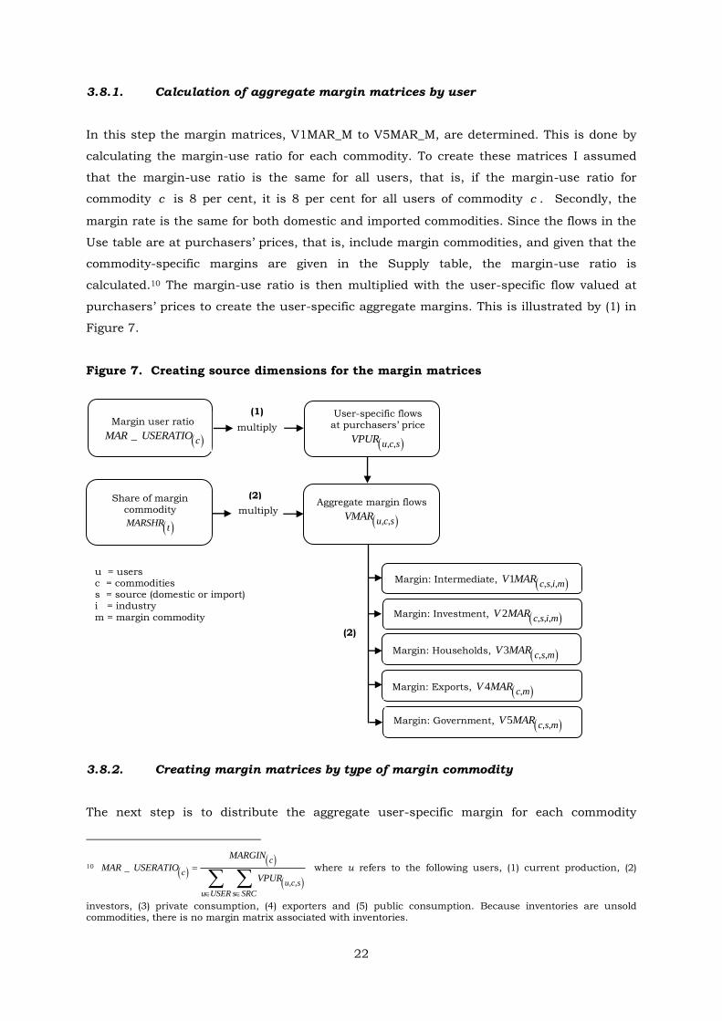
3.8.1. Calculation of aggregate margin matrices by user
In this step the margin matrices, V1MAR_M to V5MAR_M, are determined. This is done by
calculating the margin-use ratio for each commodity. To create these matrices I assumed
that the margin-use ratio is the same for all users, that is, if the margin-use ratio for
commodity c is 8 per cent, it is 8 per cent for all users of commodity c . Secondly, the
margin rate is the same for both domestic and imported commodities. Since the flows in the
Use table are at purchasers’ prices, that is, include margin commodities, and given that the
commodity-specific margins are given in the Supply table, the margin-use ratio is
calculated.10 The margin-use ratio is then multiplied with the user-specific flow valued at
purchasers’ prices to create the user-specific aggregate margins. This is illustrated by (1) in
Figure 7.
Figure 7. Creating source dimensions for the margin matrices
3.8.2. Creating margin matrices by type of margin commodity
The next step is to distribute the aggregate user-specific margin for each commodity
10
c
c
u c s
u USER s SRC
MARGIN
MAR USERATIOVPUR
, ,
_ where u refers to the following users, (1) current production, (2)
investors, (3) private consumption, (4) exporters and (5) public consumption. Because inventories are unsold commodities, there is no margin matrix associated with inventories.
(2)
u = users c = commodities s = source (domestic or import) i = industry
m = margin commodity
User-specific flows at purchasers’ price
, ,u c sVPUR
Margin user ratio
cMAR USERATIO_
multiply
(1)
Aggregate margin flows
u c sVMAR , ,
Share of margin commodity
MARSHRt
Margin: Intermediate, 1c s i m
V MAR , , ,
Margin: Households, 3c s m
V MAR , ,
Margin: Exports, 4c m
V MAR ,
Margin: Government, 5c s m
V MAR , ,
Margin: Investment, 2c s i m
V MAR , , ,
(2)
multiply
23
between transport and trade margins. Since the total value of trade and transport margins
is known, the share of trade and transport in total margin is calculated.11 Again, it is
assumed that the all users use the same proportion of trade and transport margins. The
margin commodity share is then multiplied with the aggregate user-specific margin. This
yields margin matrices by commodity, source and user for all margin commodities. This is
illustrated by (2) in Figure 7.
3.9. Step 9: Creating tax matrices
3.9.1. Defining the different taxes
Indirect taxes includes taxes on products that are payable by the user and taxes on
production that are paid by producers. The SUT contains information on both these types of
taxes. Commodity-specific taxes, payable by users, are recorded in the Supply table while
industry-specific production taxes, payable by producers, are recorded in the Use table.
Taxes on products are payable on goods and services when they are produced, delivered,
sold, transferred or otherwise disposed of by their producers and are proportional to their
production values (United Nations, 1999: 26). There is only one column in the Supply table
that reports commodity-specific taxes on products. SAGE requires the creation of user-
specific tax matrices, V1TAX to V5TAX, which implies that the values in the tax column
have to be distributed across users. This proves to be difficult because we do not know who
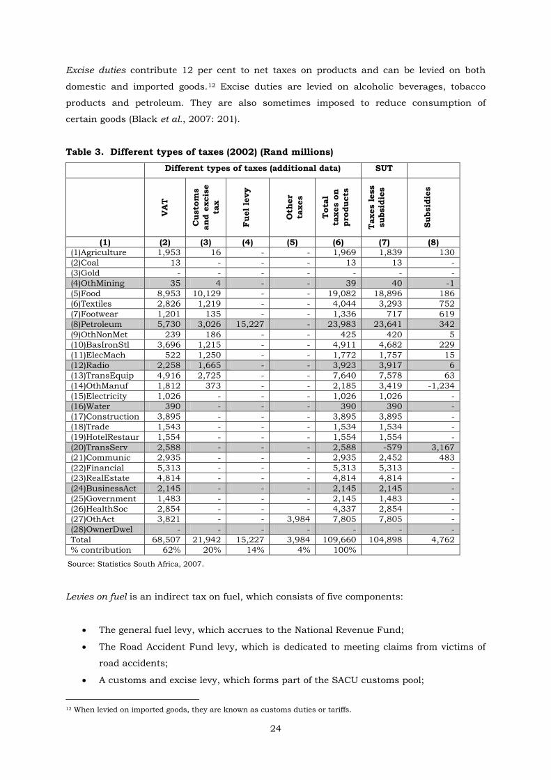
is responsible for the tax. Additional data breaks this column into four different types of
commodity taxes: VAT, customs and excise taxes, fuel levies and other taxes (Statistics
South Africa, 2007). Table 3 lists these taxes and subsidies paid on each commodity. The
row totals of the net taxes (column 7) are consistent with the data in the SUT. The elements
in columns 2 to 5 are based on expert knowledge and the column total in column 6 is
consistent with data published by the SARB (South African Reserve Bank, 2005: S-136).
VAT is by far the most important indirect tax source and contributes 62 per cent to net
taxes on products. VAT is a consumption-type tax and the revenue is raised for the
government by certain traders. These trades are registered and charge VAT on taxable
supplies for goods and services on behalf of the government. The tax burden of the tax falls
on the final consumer.
11
2
1
t
t
t
t
MARGIN
MARSHR
MARGINS
where t is the margin commodity, t = 1 (transport services) and t = 2 (trade)
24
Excise duties contribute 12 per cent to net taxes on products and can be levied on both
domestic and imported goods.12 Excise duties are levied on alcoholic beverages, tobacco
products and petroleum. They are also sometimes imposed to reduce consumption of
certain goods (Black et al., 2007: 201).
Table 3. Different types of taxes (2002) (Rand millions)
Different types of taxes (additional data) SUT
VA
T
Custo
ms
and e
xcis
e
tax
Fuel le
vy
Oth
er
taxes
Tota
l
taxes o
n
pro
ducts
Taxes less
subsid
ies
Subsid
ies
(1) (2) (3) (4) (5) (6) (7) (8)
(1)Agriculture 1,953 16 - - 1,969 1,839 130
(2)Coal 13 - - - 13 13 -
(3)Gold - - - - - - -
(4)OthMining 35 4 - - 39 40 -1
(5)Food 8,953 10,129 - - 19,082 18,896 186
(6)Textiles 2,826 1,219 - - 4,044 3,293 752
(7)Footwear 1,201 135 - - 1,336 717 619
(8)Petroleum 5,730 3,026 15,227 - 23,983 23,641 342
(9)OthNonMet 239 186 - - 425 420 5
(10)BasIronStl 3,696 1,215 - - 4,911 4,682 229
(11)ElecMach 522 1,250 - - 1,772 1,757 15
(12)Radio 2,258 1,665 - - 3,923 3,917 6
(13)TransEquip 4,916 2,725 - - 7,640 7,578 63
(14)OthManuf 1,812 373 - - 2,185 3,419 -1,234
(15)Electricity 1,026 - - - 1,026 1,026 -
(16)Water 390 - - - 390 390 -
(17)Construction 3,895 - - - 3,895 3,895 -
(18)Trade 1,543 - - - 1,534 1,534 -
(19)HotelRestaur 1,554 - - - 1,554 1,554 -
(20)TransServ 2,588 - - - 2,588 -579 3,167
(21)Communic 2,935 - - - 2,935 2,452 483
(22)Financial 5,313 - - - 5,313 5,313 -
(23)RealEstate 4,814 - - - 4,814 4,814 -
(24)BusinessAct 2,145 - - - 2,145 2,145 -
(25)Government 1,483 - - - 2,145 1,483 -
(26)HealthSoc 2,854 - - - 4,337 2,854 -
(27)OthAct 3,821 - - 3,984 7,805 7,805 -
(28)OwnerDwel - - - - - - -
Total 68,507 21,942 15,227 3,984 109,660 104,898 4,762
% contribution 62% 20% 14% 4% 100%
Levies on fuel is an indirect tax on fuel, which consists of five components:
The general fuel levy, which accrues to the National Revenue Fund;
The Road Accident Fund levy, which is dedicated to meeting claims from victims of
road accidents;
A customs and excise levy, which forms part of the SACU customs pool;
12 When levied on imported goods, they are known as customs duties or tariffs.
Source: Statistics South Africa, 2007.
25
An equalisation fund levy, the proceeds of which have been used in the past to
smooth the monthly fluctuations in the domestic fuel price due to changes in
international crude oil prices; and
A small levy has been imposed as of 2001, on diesel sales to fund the marking and
dyeing of illuminating paraffin to combat the illegal mixing of diesel and illuminating
paraffin.
Other taxes include registration fees on housing, charges and levies on financial transaction,
air departure tax and social security tax charges. In 2002 the air passenger departure tax
was introduced at R50 per fee-paying passenger travelling to SACU countries13 and R100
per fee-paying passenger travelling to all other countries.
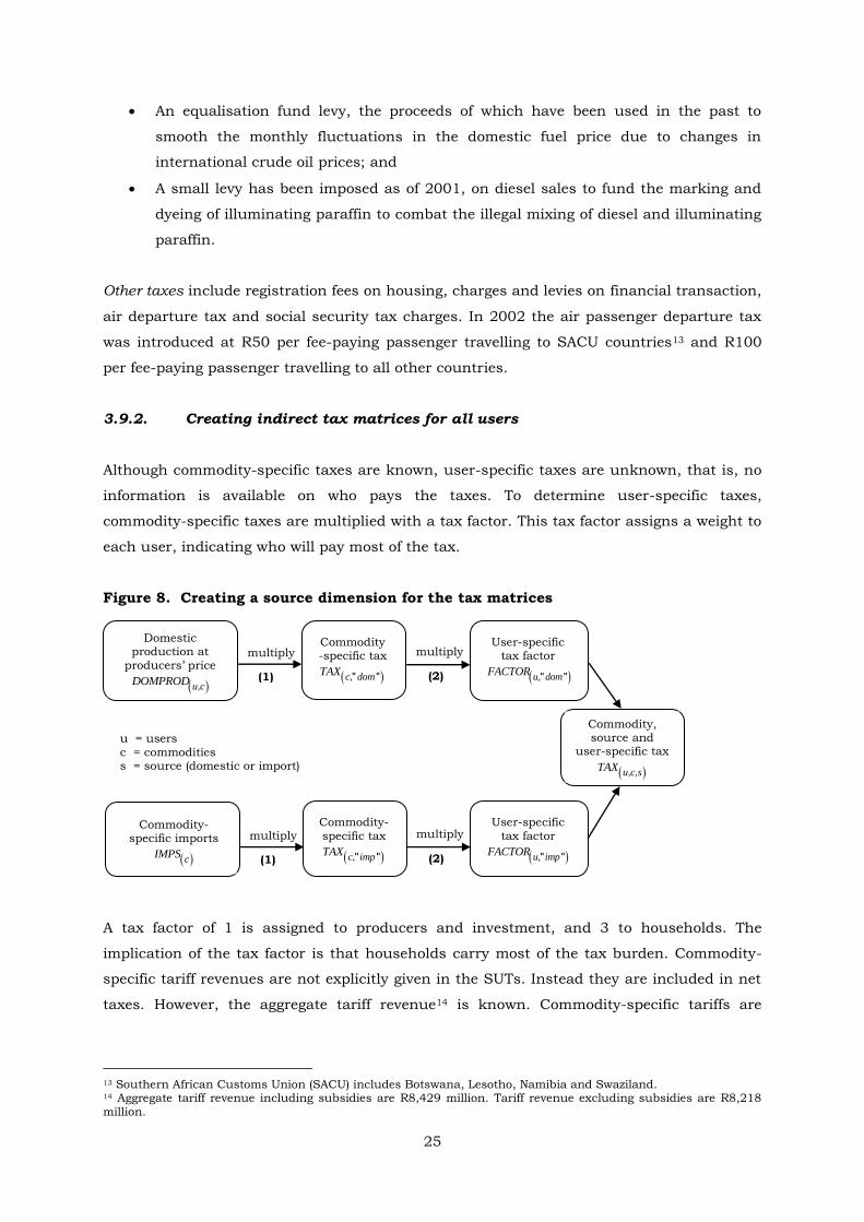
3.9.2. Creating indirect tax matrices for all users
Although commodity-specific taxes are known, user-specific taxes are unknown, that is, no
information is available on who pays the taxes. To determine user-specific taxes,
commodity-specific taxes are multiplied with a tax factor. This tax factor assigns a weight to
each user, indicating who will pay most of the tax.
Figure 8. Creating a source dimension for the tax matrices
A tax factor of 1 is assigned to producers and investment, and 3 to households. The
implication of the tax factor is that households carry most of the tax burden. Commodity-
specific tariff revenues are not explicitly given in the SUTs. Instead they are included in net
taxes. However, the aggregate tariff revenue14 is known. Commodity-specific tariffs are
13 Southern African Customs Union (SACU) includes Botswana, Lesotho, Namibia and Swaziland. 14 Aggregate tariff revenue including subsidies are R8,429 million. Tariff revenue excluding subsidies are R8,218
million.
Commodity, source and
user-specific tax
u c sTAX , ,
(2)
multiply User-specific
tax factor
u domFACTOR
," "
(1)
multiply
Domestic production at
producers’ price
u cDOMPROD
,
Commodity -specific tax
c domTAX ," "
(1)
multiply Commodity-
specific imports
cIMPS (2)
multiply Commodity-
specific tax
c impTAX
," "
User-specific
tax factor
u impFACTOR ," "
u = users
c = commodities s = source (domestic or import)
26
determined by calculating the share of each commodity in the total Customs and excise
taxes paid (column 3 in Table 3) and multiplying this share by the total tariff revenue.
3.9.3. Taxes on production
Taxes on production consist mainly of taxes on the ownership or use of land, buildings or
other assets used in production or on the labour employed, or compensation of employees
employed. Examples of taxes on production include taxes payable by producers for business
licences, payroll taxes, stamp duties. These taxes are not proportional to the value of goods
and services produced (United Nations, 1999: 26). The industry-specific production taxes
are captured in the Use table. The production taxes, summed across industry, are
consistent with the SARB data (South African Reserve Bank, 2005: S-136). Hence, no
further adjustments are required. Taxes on production were R25,028 million and subsidies
on production R3,485 million. Therefore, net production taxes are R21,543 million. At the
end of this step, the V1TAX to V5TAX and V0TAR matrices have been created.
3.10. Step 10: Creating matrices for the basic flows
The aim of this step is to create the domestic flow values of the BAS1 to BAS6 matrices.
These flows are illustrated in the first row of Figure 1. The flows at purchasers’ price include
the basic value plus the margin costs plus taxes. The imported flows at basic prices are
calculated in Step 6, margin flows in Step 8 and tax matrices in Step 10. Based on the
outcomes of these steps, the domestic flows valued at basic prices are determined.
To calculate the domestic basic flows, I subtract the imports, margin and tax flows from the
total purchases values:
, , , , , ,
, , , , ,
u c dom u c s u c imp
s SRC
u c s m u c s
s SRC m MAR s SRC
BAS VPUR BAS
MAR TAX
(E4.5)
At the end of this step the domestic flows of the V1BAS to V6BAS matrices are created.
3.11. Step 11: Creating an industry dimension for the investor column
Currently, the matrices pertaining to investors (user 2) are vector matrices implying that
there is only one representative investor. This is consistent with the investment data
included in the SUT. However, we know that investors buy commodities to construct capital
27
in each industry. The aim in this step is two-fold. Firstly, the amount of investment
undertaken by each industry is calculated. The sum of all the industry investment should
be consistent with the economy-wide investment. Secondly, for each industry the
commodity-composition is determined. The total use of each commodity for investment
purposes summed across all industries, should add up to the value of the commodity-
specific investment as it appears in the official data. To determine the required investment
data, I follow the work by Giesecke and Tran (2007). They use the Capital Asset Pricing
Model (CAPM) theory to create the necessary data for a dynamic model for Vietnam. The
next section relies heavily on their description of determining the required investment data
(Giesecke & Tran, 2007).
3.11.1. Calculating industry-specific investment
No official industry-specific investment data are available to split the aggregate investment
column into 28 columns. Instead, industry-specific investment is determined from assumed
capital growth rates, depreciation rates and rates of return.
Capital accumulates over time according to the following formula:
1 0 1i i i i
K K d I (E4.6)
where 0
iK and 1
iK are the industry-specific capital stock at the beginning and
the end of the year;
iI is investment undertaken by industry during the year; and
id is the industry-specific depreciation rate.
Rewriting (E4.6) yields:
0i i i i
I K k d (E4.7)
where k is the growth rate of capital stock in an industry:
1 0
0
i i
ii
K Kk
K
(E4.8)
If the values of 0
K , k and d were known, I could be calculated via (E4.7). However, no
industry-specific data are available for these variables. There is, however, data on industry-
28
specific gross operating surplus (V1CAP). The industry-specific V1CAP can be used to infer
industry-specific investment via the rate of return on capital. The net rate of returns on
capital is:
1 1 0
2 * 0 2 0
i i i
i i ii i i i
V CAP P cap KR d d
P tot K P tot K (E4.9)
where iR is the net rate of return on industry-specific capital;
1V CAP is the industry-specific gross operating surplus (capital
rentals);
2 iP tot is the cost of building a new unit of capital; and
1 iP cap is the industry-specific gross return per unit of capital.
From (E4.7) and (E4.9) we have:
1i i i
ii i
V CAP k d
IR d
(E4.10)
Equation (E4.10) shows that to calculate industry-specific investments, the following
information is required:
1V CAP , which is known from the Use table;
ik is the industry-specific capital growth rates;
id is the industry-specific depreciation rates; and
iR is the industry-specific rates of return on capital.
The remainder of this subsection describes the method of calculating d , k and R .
3.11.1.1. Calculating industry-specific depreciation rates d
As a first guess, the economy-wide average depreciation rate for 2002 can easily be
calculated from data published by the SARB. The economy-wide depreciation rate, based on
SARB published data, is calculated via (E4.11) at 7.2 per cent:
*100 D
dVCAP
(E4.11)
29
where d is the economy-wide depreciation rate;
D is the published total depreciation value at current price; and
VCAP is the published total capital stock.
The SARB does not publish data on industry-specific depreciation rates and capital stocks. I
therefore use a second data source, QUANTEC. QUANTEC publishes data on capital stocks
and consumption of fixed capital for selected industries. To determine the industry-specific
depreciation values, net fixed investment is calculated as:
1 0i i i i
K K I D (E4.12)
where 0i
K and 1i
K are the capital stock at the beginning and the end the year ;
iI is gross domestic fixed investment undertaken during the year; and
iD is the depreciation value and calculated as 0i id K* where id is the
depreciation rate.
From (E4.12) net domestic fixed investment ( )t t
I D is calculated as the difference between
the start 1K and the end 0K capital stock data. The depreciation value at constant price
can now be calculated as the difference between gross domestic fixed investment and net
domestic fixed investment. This can then be transformed into a depreciation value at
replacement cost by multiplying by the appropriate investment deflator. These rates vary
across industries. Reasons for the differences in depreciation rates include: (1) different
economic lives for the different assets used by industries and (2) industries using different
combinations of capital assets. The current estimate of economic lifetimes for the different
types of assets in South Africa varies between a maximum of 80 years for construction
works and eight years for the transport equipment (SAICA, 2007). For Owner Dwellings the
depreciation rate is set at 2 per cent.
The dispersion among the industry-specific depreciation rates is adjusted according to
(E4.13):
, *
i
adj i aveave
dd d
d
(E4.13)
where id and ,adj id are the depreciation rates of industry 'i s capital stock
30
before and after the adjustment;
aved is the average economy-wide depreciation rate at 6 per cent; and
us the adjustment coefficient, which is set at 0.5.
The final depreciation rates vary between 6 and 10 per cent for manufacturing industries
and 4 and 9 per cent for service industries. The weighted average depreciation rate for the
economy is 6.1 per cent.
3.11.1.2. Calculating industry-specific capital growth rates k
The economy-wide capital growth rate, based on the SARB data, is calculated as the
percentage change in capital stock from 2001 to 2002. The capital growth rate is 1.09 per
cent (South African Reserve Bank, 2005: S-129). As with the depreciation rate, the SARB
does not publish industry-specific capital growth rates. Based on data from QUANTEC, the
industry-specific capital growth rates are calculated. Capital growth rates vary across
industries. Other mining, Health and Social work, Owner dwelling and Communications all
indicate strong positive capital growth while Coal, Food, Textiles, Electricity and Water all
indicate negative growth rates. For all the negative capital growth rates, I assigned a small
positive default value of 0.002. The dispersion of the capital growth rates across all
industries was reduced via:
, *
i
adj i aveave
kk k
k
(E4.14)
where ik and ,adj ik are the capital growth rate before and after the adjustment
for year t ;
avek is the average economy-wide capital growth rate at 3.2 per cent period
t ; and
is the adjustment coefficient which is set at 0.5.
I then scale the industry-specific capital growth rates so that their rental-weighted average
is equal to the growth rate of the aggregate capital stock of 1.2 per cent.
3.11.1.3. Calculate industry-specific rates of return R
I do not have any plausible independent data that can be used to determine R in (E4.10).
Following Giesecke and Tran (2007), I use the following steps to determineR :
31
Firstly, the industry-specific normal rate of return to equity is calculated by the CAPM
equation:
equity f m f
iiR R R R (E4.15)
where
equity
iR is the return on industry 'i s equity;
f
R is the return on a risk-free investment. The interest rate on
government 10 year bond as a proxy;
m
R is the average market equity rate of return; and
m f
i R R is the risk premium on equity capital in industry i .
Secondly, I assume that the normal rate of return on capital nor
iR in industry i is the
weighted average cost of capital:
1 nor equity equity equity f
ii i i iR S R S R (E4.16)
where i is the premium above the risk-free rate that an industry will pay
on debt finance; and
equity
iS is the share of equity in industry 'i s capital financing
structure.
Thirdly, I assume that fast-growing industries will have actual rates of return that exceed
nor
iR :
, ,_nor
i adj i adj iiR R k k trend (E4.17)
where ,_ adj ik trend is the trend growth rate of capital stock in industry i over a
historical period of time and scaled to the economy-wide average.
Calculating the rate of return on industry equity
To calculate the rate of return on industry equity, equity
iR , in (E4.15), the following
assumptions are made:
32
The risk-free return, f
R , is set at 10.4 per cent. This was the nominal
fixed interest rate on the South African government 10-year bond (SARB
S-29).
The market rate of return, m
R , is set at 15.1 per cent.
Independent industry-specific values for Beta were not available for
South Africa. Assumed values for Beta were calculated as follows. First, I
assign a risk index to each industry based on informal knowledge about
the volatility and profitability of these industries. The risk index varies
from 1 to 11, with 6 the average (Table 4.5). With each risk level, I assign
a value to link the risk level with the i values. The values are listed in
Table 4.5. Low-risk industries (risk index of 1–3) include Owner
Dwellings, Electricity, Water, General Government, Health and social
work and Other activities and services. High-risk industries (risk index of
8–11) include Real Estate and Business Activities, Mining, Petroleum,
and Hotels and Restaurants. Appendix 4H, columns (4), lists the
assigned values for the industry-specific i .
Table 4. The values assigned to the risk index
Risk index 1 2 3 4 5 6 7 8 9 10 11
i 0.50 0.63 0.78 0.88 0.95 1.00 1.05 1.12 1.22 1.37 1.50
Given all the above information, equity
iR is calculated via (E4.15).
Calculating the normal rate of return on industry capital stock
Calculating the normal rate of return on industry capital stock, nor
iR , via (E4.16), requires
information on the shares of equity and debt in total assets in each industry. This is
calculated from data on the capital resources of enterprises (Statistics South Africa, 2006a).
Assuming that the corporate debt premium is 3 per cent, nor
iR is calculated via (E4.16).
This procedure determines an economy-wide rental-weighted average cost of capital of 15.1
per cent.
Source: Adapted from Giesecke and Tran, 2007: 40.
33
Calculating trend capital growth rates
To adjust nor
iR via (E4.17), I require industry-specific trend capital growth rates. Given that
target trend growth rate, _k tot , is set at 1.1 per cent, the dispersion in the trend rates is
reduced via:
,
1 * _
_ _ *1 * _
i
i INDadj i i
i i
i IND
V CAP k tot
k trend k trendV CAP k trend
(E4.18)
Finally, industry-specific investments are calculated by substituting (E4.17) with (E4.10):
1
, ,_
i i i
i nor
adj i adj i ii
V CAP k d
I
R k k trend d
(E4.19)
3.11.2. Completing the investment matrix
The process described above determines the value of investment by each SAGE industry.
Combined with commodity-specific investments (row totals), the task now is to complete the
investment matrix by calculating the share of each commodity used by the different
industries. Every industry has a unique input requirement. This requirement depends on
the nature of the industry. For example, the transport services industry will mainly invest in
transport equipment.
No data are available on industry use of commodities. I therefore adopt the industry-specific
input requirements, that is, the share of commodities used by each industry for investment
purposes, from the Australian dynamic CGE model (MONASH). The MONASH commodity
and industries are mapped to the 28 SAGE commodities and industries. I then calculate the
share of commodity inputs to each industry’s capital formation. These shares are then
multiplied with the aggregate industry-specific investment calculated via (E4.19). The final
step is to balance the investment matrix.
3.11.3. Determining industry-specific capital stocks
With known values for, iI , ik and id , industry-specific capital stocks iK can be
calculated via (E4.7). The aggregate value of capital stock is estimated to be R2,547,110
34
million. This implies an investment-capital ratio of 0.7 and a capital-output ratio of 2.18.15
These ratios are plausible values for a developing country like South Africa.
3.12. Step 12: Final balancing of the SAGE database
The database created using Steps 1–11, creates minor distortions. For the SAGE database
to be balanced, two conditions have to be satisfied.
3.12.1. Condition 1: industry costs should equal industry output
We assume that no pure economic profits are made by the industries and therefore the first
condition states that industry costs should equal industry output. This means that when
considering Figure 1, the column totals for each industry in the producer column (column
1), should be equal to the domestic output of each industry:
_ _ i iIND COSTS IND OUTPUT (E4.20)
where
, , , , ,
, , ,
_ 1 1
1 1
1 1 0 1
i c s i c s i mc COM s SRC c COM s SRC m MAR
c s i i oc COM s SRC o OCC
i i i i
IND COSTS V PUR V MAR
V TAX V LAB
V CAP V LAND TAX V OCT
(E4.21)
and
,_ = i i cc COM
IND OUTPUT MAKE
(E4.22)
where iIND COST_ is total cost of each industry;
, ,1 c s ic COM s SRC
V PUR
is the basic intermediate flows to all industries summed
across all commodities and sources;
, , ,1 c s i mc COM s SRC m MAR
V MAR
is the total margins used to facilitate flows to
industries, summed across commodities, sources and types of margins;
,1 i oo OCC
V LAB
is the compensation of employees summed across all
15 GDP is R1,168,778 million.
35
occupations;
1 iV CAP is the industry-specific gross operating surplus;
1 iV LAND is the rental value of land for the agricultural and mining
industries;
0 iTAX is the industry-specific production taxes;
1 iV OCT is industry-specific other cost tickets;
_ iIND OUTPUT is the total industry output; and
,i cc COM
MAKE
is the total industry output summed across commodities.
3.12.2. Condition 2: domestic commodity output equals total use
We assume that all markets clear and therefore the second condition states that domestic
commodity output should equal total use:
_ _ c cCOM OUTPUT COM USE (E4.23)
where
,_
c i ci IND
COM OUTPUT MAKE (E4.24)
For non-margin commodities the _ cCOM USE is:
1 2
3 4 5
6
," ", ," ",
," " ," "
," "
_
c c dom i c dom i
i IND i IND
c dom c c dom
c dom
COM USE V BAS V BAS
V BAS V BAS V BAS
V BAS
(E4.25)
For margin commodities the _ cCOM USE is:
1 2
3 4 5
," ", ," ",
," " ," "
, , , ,
_
m m dom i m dom i
i IND i IND
m dom m m dom
u c s i m
c COM u USER s SRC i IND
COM USE V BAS V BAS
V BAS V BAS V BAS
VMAR
(E4.26)
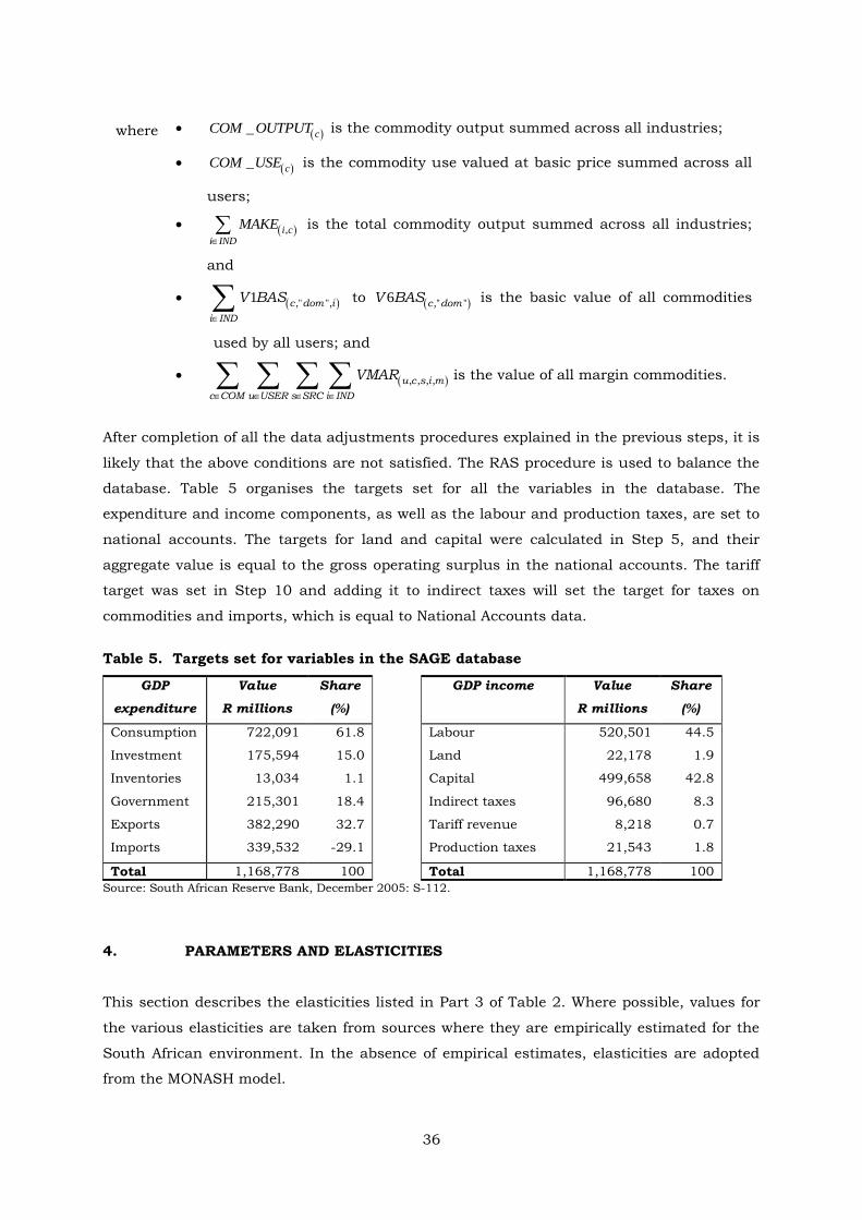
36
where _ cCOM OUTPUT is the commodity output summed across all industries;
_ cCOM USE is the commodity use valued at basic price summed across all
users;
, i ci IND
MAKE
is the total commodity output summed across all industries;
and
1 ," ",
c dom i
i IND
V BAS to 6 ," "c domV BAS is the basic value of all commodities
used by all users; and
, , , ,
u c s i m
c COM u USER s SRC i IND
VMAR is the value of all margin commodities.
After completion of all the data adjustments procedures explained in the previous steps, it is
likely that the above conditions are not satisfied. The RAS procedure is used to balance the
database. Table 5 organises the targets set for all the variables in the database. The
expenditure and income components, as well as the labour and production taxes, are set to
national accounts. The targets for land and capital were calculated in Step 5, and their
aggregate value is equal to the gross operating surplus in the national accounts. The tariff
target was set in Step 10 and adding it to indirect taxes will set the target for taxes on
commodities and imports, which is equal to National Accounts data.
Table 5. Targets set for variables in the SAGE database
GDP
expenditure
Value
R millions
Share
(%)
GDP income Value
R millions
Share
(%)
Consumption
Investment
Inventories
Government
Exports
Imports
722,091
175,594
13,034
215,301
382,290
339,532
61.8
15.0
1.1
18.4
32.7
-29.1
Labour
Land
Capital
Indirect taxes
Tariff revenue
Production taxes
520,501
22,178
499,658
96,680
8,218
21,543
44.5
1.9
42.8
8.3
0.7
1.8
Total 1,168,778 100 Total 1,168,778 100
Source: South African Reserve Bank, December 2005: S-112.
4. PARAMETERS AND ELASTICITIES
This section describes the elasticities listed in Part 3 of Table 2. Where possible, values for
the various elasticities are taken from sources where they are empirically estimated for the
South African environment. In the absence of empirical estimates, elasticities are adopted
from the MONASH model.
37
In reviewing the elasticities adopted in this study, I focus on two econometric studies. Van
Heerden and Van der Merwe (1997) estimated elasticities that were adopted in IDCGEM, the
Industrial Development Corporation’s (IDC) CGE model. Before their estimations, elasticities
in IDCGEM were adopted from the MONASH model. In their study, the estimations are
based on annual data for 25 manufacturing sectors for the period 1973–1993. For the
majority of the manufacturing sectors, the results were statistically significant with the
expected sign. Most of the elasticities were found to be similar in magnitude to other
elasticities estimated by different econometric methods elsewhere (Van Heerden & Van der
Merwe, 1997). The second set of estimations was conducted by De Wet (2003). His
elasticities were adopted for a CGE model used to evaluate environmental policy (double
dividend hypothesis). He used a combination of microeconometric and econometric methods
to estimate several elasticities for 45 industries. The elasticities adopted in this study are
summarised in Appendix 2.
4.1. The substitution parameter between primary factors
The substitution parameter between primary factors indicates the ease with which an
industry can substitute away from primary input a toward primary input b , if primary
input a becomes more expensive relative to the other primary inputs. The CES specification
implies that the substitution elasticity is constant for all pair-wise substitution possibilities.
This means that the substitution elasticity between labour and capital, for all non-land
using industries, and the pairwise substitution elasticities between labour, land and capital
in each of the land-using industries are similar.
Van Heerden and Van der Merwe (1997) estimated the capital-labour substitution elasticity
for 25 manufacturing industries. The highest elasticity of substitution is 0.61 for the Other
Non-Metallic Mineral Products sector and the lowest value is 0.086 for the Basic Iron and
Steel Products sector.
De Wet estimated the substitution elasticities between capital and labour for 40 South
African industries. The average elasticity of substitution is 0.66. The elasticities vary
between the lowest value of 0.17 for Water Supply and highest value of 1.45 for the
Communications industry. De Wet assigns the average elasticity of 0.66 to industries for
which significant results could not be estimated. The elasticities indicate that most of South
Africa’s industries function at an elasticity of substitution of less than one (De Wet, 2003).
For this study, the substitution elasticity of 0.4 is adopted.
38
4.1. The CES substitution elasticities between labour occupations
The labour substitution elasticity determines the sensitivity of industry 'i s demand for a
specific occupation when there are changes in the relative price of occupations. It is very
difficult to estimate the substitution elasticities between different occupation types due to
lack of data. Dixon et al. (1982) cite a study by Ryland and Parham (1978) where the
pairwise substitution elasticities for five types of labour are estimated. Although the overall
results were not satisfactory, a value of 0.2 was obtained for the labour-labour substitution
elasticity where occupational labour inputs were combined by a CES function to generate
the overall labour input (Dixon et al., 1982: 190).
Due to institutional and structural factors that characterise the South African labour
market, one should not expect a high degree of substitution between the different types of
labour. Therefore De Wet (2003) also adopts a labour-substitution value of 0.2. The
UPGEM16 model adopts the ORANI-G17 labour-substitution elasticity of 0.5. For this study,
the MONASH value of 0.35 is adopted for the elasticity of substitution between occupations.
The elasticities are summarised in Appendix 2, column 2.
4.2. The elasticities of substitution between domestic and foreign sources
of supply
Trade theory often assumes that domestic and imported commodities are perfect
substitutes, implying that the elasticity is infinite. This, however, does not explain why there
is a demand for a specific commodity from both domestic and imported sources. This led to
the Armington assumption. The Armington assumption allows for similar commodities
produced by different countries to be imperfect substitutes, with the degree of
substitutability governed by the Armington elastisity. A high Armington elasticity implies
that an industry is more sensitive to changes in domestic and foreign prices and therefore
there is a high degree of substitution. Low elasticities imply that industries are not sensitive
to changes in relative prices and therefore there is not a very high degree of substitution
between imported and domestic commodities.
Following Dixon et al. (1982), it is further assumed that the Armington elasticity is the same
for all users, that is:
1 2 3
, ,
c i c i c for c COM and i IND . The numbers refer to the
users: (1) refers to producers, (2) investors and (3) households. Dixon et al. (1982) defend
16 UPGEM is a static CGE model for South Africa and hosted at the Department of Economics at the University of Pretoria. 17 ORANI-G is a static CGE model for Australia (Dixon et al., 1982).
39
this assumption by pointing out that most of Australia’s major imports are used
predominantly in one end-use category only (Dixon et al., 1982: 182).
For most trade policy models in South Africa, the Armington elasticities estimated by Van
Heerden and Van der Merwe (1997) are adopted. The lowest estimated elasticity is 0.57 for
the Other Non-Ferrous Metal Products sector and the highest elasticity is 4.41 for the Leather
and Leather Products sector. For some sectors the elasticity is insignificant from zero and
where elasticities are not estimated, the elasticities from the Monash model are adopted.
The high elasticity values may be attributed to the level of disaggregation of the
Manufacturing sector. The more disaggregated the sectors, the easier it is to substitute away
(towards) from domestic (imported) commodities.
De Wet (2003) estimates the Armington elasticities for 45 South African industries. For
industries where the elasticities are either not significant or do not exhibit a cointegrating
relationship, the average Armington elasticity of 0.94 is assigned. With the exception of a
few industries, most elasticities are less than 1, implying that there is not a very high degree
of substitution between imported and domestically produced commodities. De Wet argued
that the low elasticities can be attributed to the level of industry aggregation. The 45
industries can be disaggregated further, which may increase the ease of substitution
between domestic and imported commodities. The most sensitive industries are the Civil
Engineering (2.84), Leather (1.83), Building and Construction industries (1.57). The least
sensitive industries are the Glass (0.35) and Coke (0.47) (De Wet, 2003).
The final South African study under consideration is that of Gibson (2003) where Armington
elasticities for 42 industries are estimated. Out of the total, 32 exhibit positive and
significant short-term Armington elasticities. The most sensitive sectors are the Coal Mining
(2.771), Footwear (2.04), Beverages (1.57), Leather and Leather products (1.474). The least
sensitive sectors are the Catering and Accommodation services (0.42), Basic Chemicals
(0.677) and Coke and Refined Petroleum products (0.73) (Gibson, 2003: 17).
The GTAP database, version 6.0, includes Armington elasticities for South Africa for 57
sectors (Dimaranan, 2006). The highest elasticity is 17.20 for the Gas sector and the lowest
elasticity is 0.9 for the Other Non-Metal sectors.
Comparing the results from the above-mentioned four sources, shows that no obvious
pattern can be observed. The only observation is that the GTAP elasticities seem to be
higher than the South African estimated elasticities. The implication is that careful
consideration should be given if elasticities are adopted from international studies. The
reason is that economic structure and policy may differ between countries. In addition to
international comparisons, estimates from South African studies yield very different results.
40
Some of the reasons Gibson (2003) cites are (1) the IDC report estimates Armington
elasticities for only intermediate goods while the Gibson study uses data for total
production; (2) data may be unreliable and inconsistent; and (3) different econometric
methodologies may be used. For further discussion on this topic, see Gibson (2003), Section
6.2. The Armington elasticites used in this study are adopted from Gibson and reported in
Appendix 2, column 4.
4.3. The Constant Elasticity of Transformation (CET elasticity)
SAGE allows for industries to produce more than one product. For these industries, a CET
product transformation elasticity has to be specified. In a study by Pauw and Edwards
(2006), where they evaluate the effects of a wage subsidy scheme for South Africa, a CET of
2 is adopted. The UPGEM model adopts a CET of 0.5 and GTAP reports an elasticity of 0.4.
For the purpose of this study, a CET elasticity of 0.5 is adopted. These elasticities are
summarised in Appendix 2, column 3.
4.4. Export demand elasticities
The export demand elasticities are important in determining the sensitivity of exports to a
change in relative prices. A change in the price of exports 4c
p will not only affect the
value of exports 4c
w and the balance of trade, but also the terms of trade and the welfare
of a country.
In 2008, South Africa’s share in world exports was 0.5 per cent (World Trade Organisation,
2010). Therefore, South Africa is considered to be a small open economy and lacks pricing
power in international markets. For this reason, De Wet (2003) did not estimate export
elasticities and assumed a value of -4 for all common export commodities. The export
elasticities estimated by Van Heerden and Van der Merwe (1997) show the highest elasticity
for Beverages, and the lowest for Machinery and Equipment products (Van Heerden & Van
der Merwe, 1997: 50). For all other non-traditional export commodities a value of -1 is
adopted. For all traditional exports, except Gold Mining, elasticities of -3 are adopted. For
Gold Mining an export elasticitiy of -100 is adopted (South Africa has a large share in gold
exports). The UPGEM model adopts an elasticity of -5 for all traditional and non-traditional
commodities. The GTAP database implies elasticities from -34 for Gas to -1.8 for Other Metal
NEC. In this study, the elasticities for all products, except Owner Dwellings, are assumed to
be -5. For Owner Dwellings the elasticitiy is zero. These elasticities are summarised in
Appendix 2, column 5.
41
4.5. The household expenditure and marginal budget shares
For this study, the household expenditure elasticities estimated by De Wet (2003) are
adopted. De Wet estimated elasticities for 39 commodities. For commodities where the
elasticities are not significant or do not form a cointegrating relationship, the average
elasticity is assigned. The elasticities are then scaled to satisfy the Engel aggregation
property of demand systems. This property is one of the conditions in the initial database
that should not be violated, and states that the sum of the products of each income
elasticity multiplied with its budget share must equal unity. This implies that:
1 c c
c COM
EPS
(E4.27)
with
3
3
c
c
c
c COM
V PUR
V PUR
(E4.28)
where c is the average budget share of commodity c consumed by household
cEPS is the commodity-specific expenditure elasticities.
By definition, the expenditure elasticity for commodity c can be calculated as:
c c c
cc c c
x x py yE
y x y x p (E4.29)
where cx is the demand of commodity c ;
y is the household expenditure; and
cp is the price of the commodity c .
By rewriting the above equation it is clear that the expenditure elasticity is equal to the ratio
between the marginal budget share
c cx p
y and average budget share,
c cx p
y. In SAGE,
elasticities are calculated during simulations by taking the average budget shares from the
household data and by reading in the marginal budget shares. Hence, it is the marginal
budget shares and not the elasticities that form part of the dataset. However, literature only
42
reports income elasticities and not marginal budget shares. Since I know the elasticities and
the average budget shares, the marginal budget shares can be calculated as:
c c
c c c
x pE S
y
* (E4.30)
4.6. Frisch parameter
The linear expenditure system distinguishes between luxury and subsistence demand. It is
therefore necessary to determine the ratio of household luxury expenditure to total
expenditure. The Frisch parameter is the negative of the ratio between total final household
expenditure and luxury expenditure. We can expect that if household income increases, the
proportion spent on subsistence will decrease and luxury spending should increase. As a
result, we expect that the Frisch parameter for:
high-income countries to be low; and
low-income countries to be high.
Both De Wet (2003) and the UPGEM model adopt a value of -1.82 for the Frisch parameter.
The Frisch parameter reported in the GTAP database is -3.25.
For SAGE, I estimate the Frisch parameter for South Africa at -2.8. To derive the parameter,
household expenditure data from the Income and Expenditure Survey (IES) (Statistics South
Africa, 2008b) are used. The Engel law states that as income increases, the proportion of
income spent on food declines. At the same time, the proportion of income spent on
subsistence commodities will decline, that is, as income increases more income is spent on
luxury items.
Given the income and expenditure data, I assign a percentage that each expenditure group
will spend on necessities and luxuries. On this basis I calculate the average share of
subsistence expenditure in total expenditure to be 64.3 per cent and the share of luxury
spending to be 35.7 per cent. From this, the average Frisch parameter for the household
expenditure groups can be calculated as -2.80.18
18 The Frisch parameter is calculated as 100
%
luxury epending, which is
1002 80
35 73.
. .
43
5. ADDITIONAL DATA REQUIRED FOR THE DYNAMIC EQUATIONS
5.1. Investment and capital stock
The data estimated for industry-specific capital stock, depreciation rates and trend growth
rates of capital are discussed in Section 2.4.11. This section describes additional
information, not yet discussed, on how capital adjusts over time. This includes the
difference between maximum and trend growth rates of capital, the average sensitivity of
capital growth to changes in expected rates on capital, industry asset price of capital, the
level of CPI and the real interest rate.
5.1.1. Difference between maximum and trend growth rates of capital
The difference between maximum and trend growth rates of capital is set equal to a fixed 10
per cent for all industries.
5.1.2. Real interest rate
The real interest rate is needed to calculate the expected rates of return on industry capital.
The real interest rate for 2002 is 5 per cent.
5.1.3. Asset price of capital
The level of capital asset prices for all industries is normalised at 1 in the base year.
5.1.4. The average sensitivity of capital growth to changes in expected rates of
return
The average sensitivity of capital growth to changes in expected rates of return is set at 1.0.
This value is adopted from the MONASH database.
5.1.5. CPI and lagged CPI
The SARB provides information on the nominal and real data for private household
expenditure. The private consumption price deflators serve as a proxy for the CPI and the
lagged CPI. The CPI and lagged CPI are obtained from the Quarterly Bulletin and set to 1 and
0.939 (South African Reserve Bank, 2005: S–144).
44
5.2. Government accounts
The South African public sector comprises different spheres. At the core we have the central
government, which includes the governmental departments (national government), extra-
budgetary agencies and social security funds. The next sphere is the general government,
which includes the departments of the provincial and local governments to the central
government. The final sphere is the public sector, which includes the general government
and all public corporations. The largest sphere is the general government and therefore the
data for the general government, as listed in the SARB Quarterly Bulletin, are used for this
study.
5.2.1. Revenue and expenditure items
Government revenue and expenditure for 2002 are set out in Table 6. There are three main
sources of data. Firstly, Statistics South Africa publishes a detailed account of the total
consolidated expenditure by the general government but not the consolidated income19
(Statistics South Africa, 2004). They also construct the SUT and SAMs (Statistics South
Africa, 2006b & 2006c). Secondly, information on the consolidated account of the general
government is published by Treasury in the Budget Review (National Treasury, 2004: 69).
Finally, the Quarterly Bulletin, published by the SARB, includes data on public
consumption, net taxes on products and production taxes. It should be noted that there are
discrepancies between the different data sources. I therefore use, as the main source for the
income and expenditure data, the Quarterly Bulletin (South African Reserve Bank, 2005: S–
136), as it was the most consistent with the data in the SUTs.
Revenues include indirect taxes, direct taxes and other government revenue. Indirect taxes
include all taxes on commodities and imports as well as production tax. This information is
in the SUTs and Quarterly Bulletin, and the tax flows were constructed in Step 9. Direct
taxes include taxes on income and wealth and refer to tax collected from labour and capital
income. Other government revenues include income from property, that is, interest and rent
receipts as well as other revenues from households, business and the rest of the world.
Expenditures include public consumption, public investment and transfers. Transfers
consist of benefits and net interest payment. Benefits refer to social benefits paid and other
miscellaneous current transfers. Public investment is calculated as the residual as no data
is available. The following section includes explanations of more specific items in the
government account. The government deficit is 1 per cent of GDP.
19 Until 2006 only the consolidated expenditures of the general government were published in Statistical release
number P9119. As of 2006, both the consolidated expenditures and income are published.
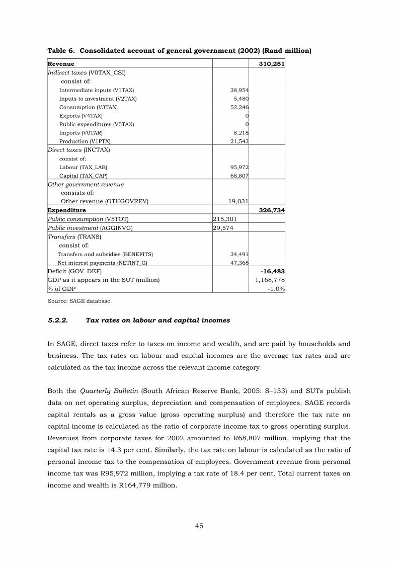
45
Table 6. Consolidated account of general government (2002) (Rand million)
Revenue 310,251
Indirect taxes (V0TAX_CSI)
consist of:
Intermediate inputs (V1TAX) 38,954
Inputs to investment (V2TAX) 5,480
Consumption (V3TAX) 52,246
Exports (V4TAX) 0
Public expenditures (V5TAX) 0
Imports (V0TAR) 8,218
Production (V1PTX) 21,543
Direct taxes (INCTAX)
consist of:
Labour (TAX_LAB) 95,972
Capital (TAX_CAP) 68,807
Other government revenue
consists of:
Other revenue (OTHGOVREV) 19,031
Expenditure 326,734
Public consumption (V5TOT) 215,301
Public investment (AGGINVG) 29,574
Transfers (TRANS)
consist of:
Transfers and subsidies (BENEFITS) 34,491
Net interest payments (NETINT_G) 47,368
Deficit (GOV_DEF) -16,483
GDP as it appears in the SUT (million) 1,168,778
% of GDP -1.0%
5.2.2. Tax rates on labour and capital incomes
In SAGE, direct taxes refer to taxes on income and wealth, and are paid by households and
business. The tax rates on labour and capital incomes are the average tax rates and are
calculated as the tax income across the relevant income category.
Both the Quarterly Bulletin (South African Reserve Bank, 2005: S–133) and SUTs publish
data on net operating surplus, depreciation and compensation of employees. SAGE records
capital rentals as a gross value (gross operating surplus) and therefore the tax rate on
capital income is calculated as the ratio of corporate income tax to gross operating surplus.
Revenues from corporate taxes for 2002 amounted to R68,807 million, implying that the
capital tax rate is 14.3 per cent. Similarly, the tax rate on labour is calculated as the ratio of
personal income tax to the compensation of employees. Government revenue from personal
income tax was R95,972 million, implying a tax rate of 18.4 per cent. Total current taxes on
income and wealth is R164,779 million.
Source: SAGE database.
46
5.2.3. Transfers
Transfers include net payments to households and the rest of the world as well as interest
paid on public debt. Net payments to households mainly consist of social benefit payments.
For 2002 the value amounts to R34,491 million. Interest payments on public debt amounts
to R47,368 million (South African Reserve Bank, 2005: S–55).
5.2.4. Public sector debt and interest paid on public sector debt
Both the South African Reserve Bank and Treasury, as part of the Budget Review, publish
data on public sector debt. For 2002 the total government debt amounted to R460,199
million. Domestic debt consists of various marketable and non-marketable bills and bonds
(South African Reserve Bank, 2005: S–59). Other debts are a very small part of total debt
and include liabilities assumed by national government from the former TBVC (Transkei,
Bophuthatswana, Venda and Ciskei) countries, self-governing territories and former regional
authorities (South African Reserve Bank, 2005: S–59). Interest paid on public sector debt
amounted to R47,368 million, which was 4.5 per cent of the GDP (South African Reserve
Bank, 2005: S–55).
5.2.5. Government investment
Government capital investments mainly consist of the acquisition of infrastructure. Due to
the lack of detailed government investment per industry, I used the MONASH shares for
government investment to distribute aggregate capital investments. As in previous steps, the
SAGE industries are mapped to the MONASH industries. The share for 28 SAGE industries
is then calculated and used to distribute government investment across all industries.
Government investments are highest in government activities such as health (27 per cent),
electricity (13.4 per cent), transport (12.8 per cent) and telecommunications (8 per cent).
5.3. Accounts with the rest of the world
The South African Reserve bank published data on the balance of payments (BOP), which
corresponds with the data published in the SUT and SAM (2002). The BOP is made up of
receipts and payments with the main components being (1) imports and exports of goods
and services, (2) net income, (3) net current transfers and (4) net capital transfers. Net
income is calculated as compensation of employees, investment income and non-direct
investment. Net current transfers and net capital transfers are made to and from the central
government and other sources.
47
5.3.1. Gross national product (GNP)
Nominal GNP is defined as the difference between GDP and the interest paid on foreign debt.
In 2002 the value was R1,133,534 million, which is 97 per cent of GDP.
5.3.2. Foreign debt and the interest rate on foreign debt in the base year
Total foreign debt for 2002 was given as R375,409 million (South African Reserve Bank,
2005: S-106). The South African Quarterly Bulletin provides data on net investment income,
which includes information on dividends and interest on foreign investment. The average
interest rate on foreign debt is calculated as the ratio between the interest payments and
total stock of foreign debt. The interest was calculated as 5.3 per cent.
5.3.3. Exchange rate
The nominal exchange rate is used in SAGE to convert coefficients valued in foreign
currency to South African Rand. In the base year the exchange rate is set at 1.
6. TESTS FOR MODEL VALIDITY
Since SAGE consists of a large number of linearised equations, which have been calibrated
by a large database, it is possible that errors may occur. Errors may occur in the database,
the equations in the model or in the specification of the model closure. Following Horridge, a
number of tests are performed each time the model equations or data are changed
(Horridge, 2006: 71).
6.1. Test 1: Real and nominal homogeneity tests
After the database has been created it is useful to test the model theory with the data. One
characteristic of SAGE is that economic agents respond to changes in the relative prices and
not the absolute price level. This implies that if all exogenous nominal variables, such as the
consumer price ( 3p tot ), increase by 1 per cent, all endogenous nominal variables will
increase by 1 per cent while real variables remain unchanged.
A second characteristic is that SAGE displays constant returns to scale. This implies that if
all exogenous real variables are shocked by 1 per cent, all endogenous real variables will
increase by 1 per cent. All prices should remain unchanged.
48
The theory of the model is represented in a number of equations. Most of the equations are
written in percentage-change form. Percentage-change equations make it easier to conduct
the homogeneity tests because the exogenous percentage-change variables can directly be
shocked with 1 per cent. Other equations can be written in ordinary-change form or include
ordinary-change variables like Y . These variables are denoted by del or the letter _d
followed by the variable name. The correct shock must now be calculated. For example,
inventory changes are denoted by d_x6cs. The correct shock is 1 per cent of the basic value
of inventories, that is, 0.01*BAS6.
6.2. Test 2: GDP from the income and expenditure side should be equal
This test checks that the percentage changes in GDP from the income side and expenditure
side are the same. For this test, real household consumption is shocked with 10 per cent.
Errors in the database or in the equations may cause GDP from the income and expenditure
side to be unequal. In addition to the solution file, the simulation generates an updated
database. This updated database is used in Test 3 as the initial solution to a simulation.
6.3. Test 3: Updated database should be balanced
In this test, this updated database, produced in Test 2, is used as the initial database. By
using the updated database as the initial solution, Tests 1 and 2 are repeated. The results
should be similar to those explained in Tests 1 and 2. If not, there might be an error with
the Update statements.
6.4. Test 4: Repeat the above steps using a multistep solution method
Tests 1–3 can be repeated by breaking each simulation into a number of steps. By doing
this, more subtle errors can be identified, such as a percentage change variable that is
passing through zero or formulae are used to alter data after they have been read in.
6.5. Test 5: Explain the results
It is possible that even if the above tests were successfully performed, errors may still occur.
For example, if the export-demand elasticities in the database had the wrong sign, the
model would still pass the tests. These types of errors are only detected by careful
inspection of the results.
7. CONCLUDING REMARKS
This paper described the structure of the core CGE database developed for a CGE model for
South Africa. I explained how the published data was transformed, in 12 steps, into the

49
required format. These steps include creating industry, source and margin flows as well as
an Owner Dwelling commodity and industry. The final database was scaled as to adhere to
the conditions set for a balanced database as well as the national accounts. In addition to
the flows, parameters were specified. Together the core database and the parameters are
sufficient for static simulations. However, SAGE is a dynamic model and requires additional
information regarding capital, rates of return and government accounts. Together, the core
database, parameters and additional data form the database required for this study. The
database also passed several tests to check the validity of both the model and database.
50
REFERENCES
Black, A.B., Calitz, E., Steenekamp, T. & Associates. (2007). Public Economics (3rd ed.).
Oxford University Press.
De Wet, T.J. (2003). A CGE Model for South Africa: The Database and Elasticities. Doctoral
thesis, Chapter 8, University of Pretoria, Pretoria, South Africa. [http://upetd.up.ac.za/thesis/available/etd-06302004-
143319/unrestricted/08chapter8.pdf. Accessed in May 2006]
Dimaranan, B.V. (2006) Global trade and assistance, and production. The GTAP 6 Data Base.
Center for Global Trade Analysis, Purdue University, West Lafayette.
Dixon, P.B., Parmenter, B.R., Sutton, J. & Vincent, D.P. (1982). ORANI: A Multisectoral Model of the Australian Economy. North-Holland, Amsterdam.
Gibson, K.L. (2003). Armington elasticities for South Africa: Long and short run industry level estimates. TIPS Working Paper, 12–2003.
[http://www.tips.org.za/node/341. Accessed in March 2008]
Giesecke J.A. & Tran, N. (2007). Tax liberalisation for Vietnam, Chapter 2. A dynamic CGE model for Vietnam. Centre of Policy Studies, Monash University, Melbourne,
Australia.
Harrison, WJ. & Pearson, R.K. (1996). Computing solutions for large General Equilibrium Models using GEMPACK. Computational Economics, Volume 9: 83–127.
Horridge, J.M. (2006). ORANI-G: A Generic Single-Country Computable General Equilibrium Model. Training document prepared for the Practical GE Modelling Course,
Centre of Policy Studies, Monash University, Melbourne.
Pauw, K., and Edwards, L. (2006). Evaluating the general equilibrium effects of a wage subsidy scheme for South Africa. South African Journal of Economics, Volume
74(3): 442-462.
Pearson, R.K. (2002). Solving nonlinear economic models accurately via a linear representation. Preliminary Working Paper No. IP-55, Centre of Policy Studies,
Monash University, Melbourne.
QUANTEC. Economic data. [http://www.quantec.co.za/. Accessed in February
2008]
South African Institute for Chartered Accountants (SAICA). (2007). Legislation Handbook
2007/2008. LexisNexis, South Africa.
South African Reserve Bank. Online statistical query (historical macroeconomic timeseries
information).
South African Reserve Bank. (2005). Quarterly Bulletin. December 2005. Pretoria, South
Africa.
51
Statistics South Africa. (1993). Standard Industrial Classification of all economic activities (5th
Ed.).
[http://www.statssa.gov.za/additional_services/sic/contents.htm. Accessed in July 2007]
Statistics South Africa. (2006a). Annual Financial Statistics Survey, 2006. Statistical Release
P0021. Pretoria, South Africa.
Statistics South Africa. (2006b). Final Social Accounting Matrix, 2002. Report no. 04-03-02
(2002). Pretoria, South Africa.
Statistics South Africa. (2006c). Final Supply and Use Tables, 2002. Report no. 04-04-01
(2002). Pretoria, South Africa.
Statistics South Africa. (2007). Addressing the needs of users for the future compilation of a Social Accounting Matrix. Document received via e-mail. Pretoria, South Africa.
Statistics South Africa. (2008). Income and expenditure of household, 2005/2006. Statistical
Release P0100. Pretoria, South Africa.
United Nations. (1999). Handbook of Input-Output table compilation and analysis. Series F,
No. 74. Department for Economic and Social Affairs, Statistics Division.
Van Heerden, J. & Van der Merwe, F. (1997). Empirical Estimation of Elasticities in IDC’s General Equilibrium Model. IDC Research Paper Series, TS2/1997.
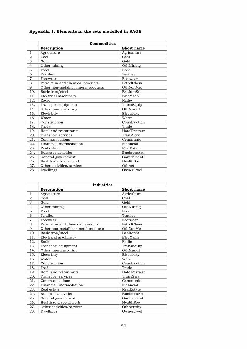
52
Appendix 1. Elements in the sets modelled in SAGE
Commodities
Description Short name 1. Agriculture Agriculture
2. Coal Coal
3. Gold Gold
4. Other mining OthMining
5. Food Food
6. Textiles Textiles
7. Footwear Footwear
8. Petroleum and chemical products PetrolChem
9. Other non-metallic mineral products OthNonMet
10. Basic iron/steel BasIronStl
11. Electrical machinery ElecMach
12. Radio Radio
13. Transport equipment TransEquip
14. Other manufacturing OthManuf
15. Electricity Electricity
16. Water Water
17. Construction Construction
18. Trade Trade
19. Hotel and restaurants HotelRestaur
20. Transport services TransServ
21. Communications Communic
22. Financial intermediation Financial
23. Real estate RealEstate
24. Business activities BusinessAct
25. General government Government
26. Health and social work HealthSoc
27. Other activities/services OthAct
28. Dwellings OwnerDwel
Industries
Description Short name 1. Agriculture Agriculture
2. Coal Coal
3. Gold Gold
4. Other mining OthMining
5. Food Food
6. Textiles Textiles
7. Footwear Footwear
8. Petroleum and chemical products PetrolChem
9. Other non-metallic mineral products OthNonMet
10. Basic iron/steel BasIronStl
11. Electrical machinery ElecMach
12. Radio Radio
13. Transport equipment TransEquip
14. Other manufacturing OthManuf
15. Electricity Electricity
16. Water Water
17. Construction Construction
18. Trade Trade
19. Hotel and restaurants HotelRestaur
20. Transport services TransServ
21. Communications Communic
22. Financial intermediation Financial
23. Real estate RealEstate
24. Business activities BusinessAct
25. General government Government
26. Health and social work HealthSoc
27. Other activities/services OthActivity
28. Dwellings OwnerDwel
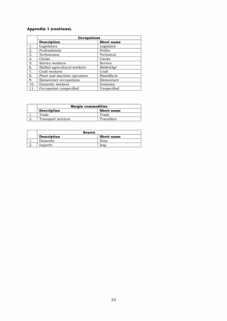
53
Appendix 1 (continue).
Occupations
Description Short name
1. Legislators Legislator
2. Professionals Profes
3. Technicians Technical
4. Clerks Clerks
5. Service workers Service
6. Skilled agricultural workers SkilledAgr
7. Craft workers Craft
8. Plant and machine operators PlantMach
9. Elementary occupations Elementary
10. Domestic workers Domestic
11. Occupation unspecified Unspecified
Margin commodities
Description Short name
1. Trade Trade
2. Transport services TransServ
Source
Description Short name
1. Domestic Dom
2. Imports Imp
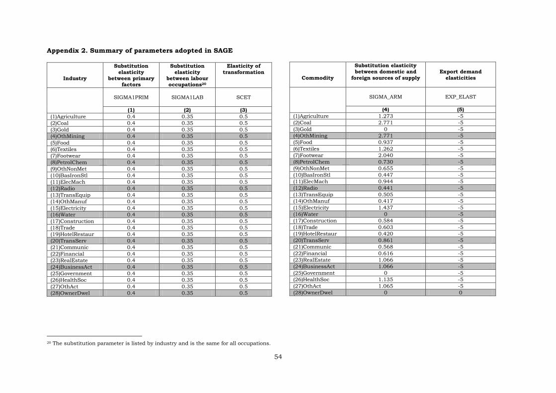
54
Appendix 2. Summary of parameters adopted in SAGE
Industry
Substitution
elasticity between primary
factors
Substitution
elasticity between labour occupations20
Elasticity of
transformation
SIGMA1PRIM
SIGMA1LAB
SCET
(1) (2) (3)
(1)Agriculture 0.4 0.35 0.5
(2)Coal 0.4 0.35 0.5
(3)Gold 0.4 0.35 0.5
(4)OthMining 0.4 0.35 0.5
(5)Food 0.4 0.35 0.5
(6)Textiles 0.4 0.35 0.5
(7)Footwear 0.4 0.35 0.5
(8)PetrolChem 0.4 0.35 0.5
(9)OthNonMet 0.4 0.35 0.5
(10)BasIronStl 0.4 0.35 0.5
(11)ElecMach 0.4 0.35 0.5
(12)Radio 0.4 0.35 0.5
(13)TransEquip 0.4 0.35 0.5
(14)OthManuf 0.4 0.35 0.5
(15)Electricity 0.4 0.35 0.5
(16)Water 0.4 0.35 0.5
(17)Construction 0.4 0.35 0.5
(18)Trade 0.4 0.35 0.5
(19)HotelRestaur 0.4 0.35 0.5
(20)TransServ 0.4 0.35 0.5
(21)Communic 0.4 0.35 0.5
(22)Financial 0.4 0.35 0.5
(23)RealEstate 0.4 0.35 0.5
(24)BusinessAct 0.4 0.35 0.5
(25)Government 0.4 0.35 0.5
(26)HealthSoc 0.4 0.35 0.5
(27)OthAct 0.4 0.35 0.5
(28)OwnerDwel 0.4 0.35 0.5
20 The substitution parameter is listed by industry and is the same for all occupations.
Commodity
Substitution elasticity between domestic and
foreign sources of supply
Export demand
elasticities
SIGMA_ARM
EXP_ELAST
(4) (5)
(1)Agriculture 1.273 -5
(2)Coal 2.771 -5
(3)Gold 0 -5
(4)OthMining 2.771 -5
(5)Food 0.937 -5
(6)Textiles 1.262 -5
(7)Footwear 2.040 -5
(8)PetrolChem 0.730 -5
(9)OthNonMet 0.655 -5
(10)BasIronStl 0.447 -5
(11)ElecMach 0.944 -5
(12)Radio 0.441 -5
(13)TransEquip 0.505 -5
(14)OthManuf 0.417 -5
(15)Electricity 1.437 -5
(16)Water 0 -5
(17)Construction 0.584 -5
(18)Trade 0.603 -5
(19)HotelRestaur 0.420 -5
(20)TransServ 0.861 -5
(21)Communic 0.568 -5
(22)Financial 0.616 -5
(23)RealEstate 1.066 -5
(24)BusinessAct 1.066 -5
(25)Government 0 -5
(26)HealthSoc 1.135 -5
(27)OthAct 1.065 -5
(28)OwnerDwel 0 0
Recommended