CONFORMAL SYMMETRY
Dissertation Reportsubmitted in partial fulfillment of the requirements for the degree of
Master of Science
in
Physics
Session: 2013 – 2014
Under the Supervision of Submitted by
Dr. Sanjay Siwach Saurav Dwivedi
Nuclear Physics Section
Department of Physics
Banaras Hindu University
Varanasi – 221005, INDIAmwww.geocities.ws/dwivedi/data/mth.pdf
Enrollment No. 300411 Roll No. 12481SC078
Certificate
This is to certify that the dissertation report entitled “Conformal Symmetry”,
submitted by Saurav Dwivedi for the award of the degree of M.Sc. in Physics
is based on original studies carried out by him under my supervision. The dis-
sertation or any part thereof has not been previously submitted for any other
degree or diploma.
Date: 15/05/2014
Place: B.H.U., Varanasi, INDIA
Dr. Sanjay Siwach
Assistant Professor
Nuclear Physics Section
Department of Physics
Banaras Hindu University

Acknowledgments
I am grateful to all my teachers, friends, and technical staff for their kind sup-
port, and encouragement.
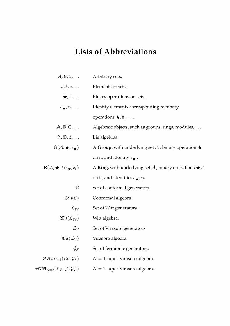
Lists of Abbreviations
A,B, C, . . . Arbitrary sets.
a, b, c, . . . Elements of sets.
F, #, . . . Binary operations on sets.
eF, e#, . . . Identity elements corresponding to binary
operationsF, #, . . . .
A, B, C, . . . Algebraic objects, such as groups, rings, modules,. . . .
A,B,C, . . . Lie algebras.
G(A;F; eF) A Group, with underlying set A , binary operationF
on it, and identity eF .
R(A;F, #; eF, e#) A Ring, with underlying set A , binary operationsF, #
on it, and identities eF, e# .
C Set of conformal generators.
Con(C) Conformal algebra.
LW Set of Witt generators.
Wit(LW ) Witt algebra.
LV Set of Virasoro generators.
Vir(LV ) Virasoro algebra.
GS Set of fermionic generators.
SVAN=1(LV ,GS) N = 1 super Virasoro algebra.
SVAN=2(LV ,J ,G±S ) N = 2 super Virasoro algebra.
Contents
1 Introduction 1
2 Conformal Symmetry 4
2.1 Conformal Symmetry in d Dimensions . . . . . . . . . . . . . . . . 5
2.1.1 Infinitesimal Conformal Transformations in d Dimensions 6
2.1.2 Conformal Algebra in d Dimensions . . . . . . . . . . . . . 7
2.2 Conformal Symmetry in d = 2 Dimensions . . . . . . . . . . . . . 9
2.2.1 Witt Algebra . . . . . . . . . . . . . . . . . . . . . . . . . . . 10
2.2.2 Virasoro Algebra . . . . . . . . . . . . . . . . . . . . . . . . 11
2.2.3 Primary Field . . . . . . . . . . . . . . . . . . . . . . . . . . 12
2.2.4 Infinitesimal Conformal Transformations of Primary Field 13
2.2.5 Highest Weight Representations (HWR) of Virasoro Algebra 14
2.2.6 Kac Determinant . . . . . . . . . . . . . . . . . . . . . . . . 15
3 Superconformal Symmetry 17
3.1 Suppersymmetry . . . . . . . . . . . . . . . . . . . . . . . . . . . . 17
3.2 Superspace . . . . . . . . . . . . . . . . . . . . . . . . . . . . . . . . 20
v
CONTENTS vi
3.3 N = 1 Super Virasoro Algebra . . . . . . . . . . . . . . . . . . . . 21
3.4 HWR of N = 1 Super Virasoro Algebra . . . . . . . . . . . . . . . 21
3.5 N = 2 Super Virasoro Algebra . . . . . . . . . . . . . . . . . . . . 22
3.6 HWR of N = 2 Super Virasoro Algebra . . . . . . . . . . . . . . . 23
4 Summary 25
Chapter1Introduction
There are two prevalent regimes in the quest of mathematization of physics,
“Symmetries” [35] and “Deformation Quantization” [4]. Former entails dynamical
invariance upon certain transformations, later deals with transmutation of theo-
ries upon deformation of their algebras. This report explores the former one,
and summarizes (Lie) algebraic aspects of conformal symmetry in d–dimensions,
and restricts it to 2–dimensions. Two-dimensional conformal symmetry entails
infinite-dimensional Lie algebras. Further, I introduce suppersymmetry, and sum-
marize Lie algebras entailing superconformal symmetry in 2–dimensions, for
minimal (N = 1) and extended (N = 2) supersymmetry, which are infinite-
dimensional as well.
Symmetry is invariance under certain structure preserving transformations1.
Simplectic systems are more symmetric than complexes. Symmetry reduces the
order of hierarchy, and thus structural organization of the theory (or model).
In mathematical argot, symmetries correspond to transformations which are
1Here, the term structure is entailed in somewhat generic sense. It could be an algebraic,
topological or a physical structure/entity, e.g. group, connectedness, mass or charge.
1
2
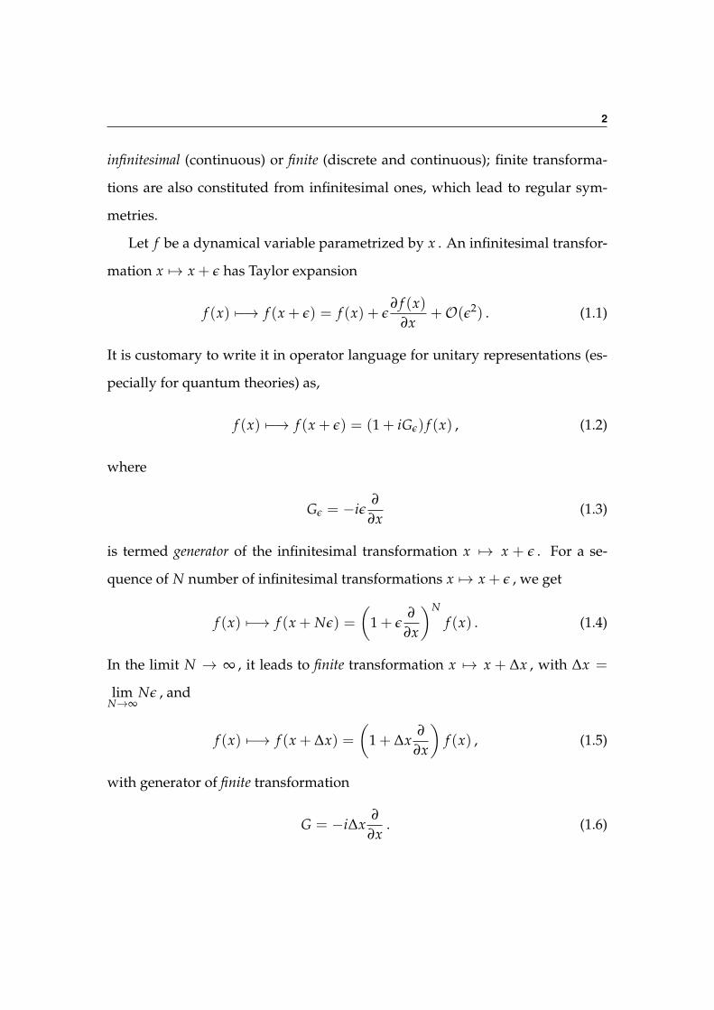
infinitesimal (continuous) or finite (discrete and continuous); finite transforma-
tions are also constituted from infinitesimal ones, which lead to regular sym-
metries.
Let f be a dynamical variable parametrized by x . An infinitesimal transfor-
mation x 7→ x + ε has Taylor expansion
f (x) 7−→ f (x + ε) = f (x) + ε∂ f (x)
∂x+O(ε2) . (1.1)
It is customary to write it in operator language for unitary representations (es-
pecially for quantum theories) as,
f (x) 7−→ f (x + ε) = (1 + iGε) f (x) , (1.2)
where
Gε = −iε∂
∂x(1.3)
is termed generator of the infinitesimal transformation x 7→ x + ε . For a se-
quence of N number of infinitesimal transformations x 7→ x + ε , we get
f (x) 7−→ f (x + Nε) =
(1 + ε
∂
∂x
)Nf (x) . (1.4)
In the limit N → ∞ , it leads to finite transformation x 7→ x + ∆x , with ∆x =
limN→∞
Nε , and
f (x) 7−→ f (x + ∆x) =(
1 + ∆x∂
∂x
)f (x) , (1.5)
with generator of finite transformation
G = −i∆x∂
∂x. (1.6)
3
Definition 1.0.1 (Continuous Symmetry). If the dynamics of any physical system
remains invariant under infinitesimal transformation of the form (1.1), or finite
transformations which are constituted from infinitesimal ones, then the system
entails continuous symmetry, and the underlying transformation is termed con-
tinuous symmetry transformation.
Examples of continuous transformations are rotation, translation, time evolu-
tion, scale transformations, gauge transformations etc.
Definition 1.0.2 (Discrete Symmetry). If the dynamics of any physical system
remains invariant under finite transformations, which are not constituted from
infinitesimal ones of the form (1.1), the system entails discrete symmetry, and the
underlying transformation is termed discrete symmetry transformation.
Examples of discrete transformations are parity transformation, charge conju-
gation, time reversal, etc.
Continuous symmetry transformations generate a class of algebras studied
by Marius Sophus Lie, called Lie algebras.
Chapter2Conformal Symmetry
Conformal symmetry is algebro-geometric symmetry. Certain transformations on
manifolds leave the geometry locally intact, termed conformal transformations.
Definition 2.0.3 (Conformality). Certain deformations of an arbitrary manifold
lead to deformed manifolds, which are locally equivalent to former’s dilatation.
Such resemblances between manifolds is termed conformality.
Definition 2.0.4 (Conformal Transformation). Transformations on a manifold,
leading to conformally equivalent manifolds, are termed conformal transfor-
mations.
Conformally equivalent manifolds are locally equivalent-upto-scaling. Ac-
tions of string models entail conformal symmetry [26, 27]. Systems entailing
conformal symmetry do not posses intrinsic length, mass, or energy scales, mak-
ing physics scale invariant. However, I restrict my approach to algebraic aspects
of conformal symmetry, rather than field theoretic.
4
2.1. CONFORMAL SYMMETRY IN D DIMENSIONS 5
2.1 Conformal Symmetry in d Dimensions
Let C be the set of transformations on a d-dimensional manifold Md , with gen-
eral metric gµν(x) (µ, ν = 0, 1, 2, . . . , d− 1) .
Definition 2.1.1 (Conformal Symmetry). Let f ∈ C . The transformation f :
Md −→M′d , leading to gµν(x) 7→ Ω(x)gµν(x) is termed conformal transforma-
tion. Manifolds Md and M′d are locally equivalent up-to-scaling, where Ω(x) is
termed scale factor. The symmetry entailed by conformal transformations C is
termed conformal symmetry.
In the argot of differential geometry, gρσ(x) transforms under x 7→ x′ , as
g′ρσ(x′) =∂xµ
∂x′ρ∂xν
∂x′σgµν(x) . (2.1)
The condition for x 7→ x′ to be conformal (i.e., local dilatation), [13, 6]
g′µν(x′) = Ω(x)gµν(x) , (2.2)
leads to,
g′ρσ(x′)∂x′ρ
∂xµ
∂x′σ
∂xν= Λ(x)g′µν(x′) , (2.3)
which is general condition for conformal symmetry, where Λ(x) = Ω−1(x) . For
flat manifolds with Lorentz metric ηµν = diag(−1, . . . ,+1, . . . ) ,
ηρσ∂x′ρ
∂xµ
∂x′σ
∂xν= Λ(x)ηµν (2.4)
is the condition for conformal symmetry on flat manifolds.
2.1. CONFORMAL SYMMETRY IN D DIMENSIONS 6
2.1.1 Infinitesimal Conformal Transformations in d Dimensions
Let Cε be set of infinitesimal conformal transformations on flat manifold Md ,
such that
x′ρ = xρ + ερ(x) +O(ε2) , (2.5)
where ε(x) 1 . Imposing condition for conformal symmetry (2.4), we get [6]
ηρσ∂x′ρ
∂xµ
∂x′σ
∂xν= ηµν +
∂εµ
∂xν+
∂εν
∂xµ +O(ε2) = Λ(x)ηµν . (2.6)
By setting
∂µεν + ∂νεµ = K(x)ηµν , (2.7)
where ∂µ := ∂∂xµ , we get
Λ(x) = 1 + K(x) +O(ε2) . (2.8)
Further, by tracing (2.7), we obtain
ηµν(∂µεν + ∂νεµ) = K(x)ηµνηµν , or (2.9)
K(x) =2d(∂ · ε) , (2.10)
where ∂ · ε = ∂µεµ . Thus, the condition for infinitesimal conformal symmetry
in d-dimensions is
∂µεν + ∂νεµ =2d(∂ · ε)ηµν , (2.11)
with scale factor Λ(x) = 1 + 2d (∂ · ε) +O(ε
2) .
We operate (2.11) by ∂ν , and sum it over ν , getting
∂ν(∂µεν + ∂νεµ
)=
2d
∂ν (∂ · ε) ηµν ,
∂µ(∂ · ε) +εµ =2d
∂µ (∂ · ε) ,(2.12)
2.1. CONFORMAL SYMMETRY IN D DIMENSIONS 7
where, = ∂µ∂µ . Operating it by ∂ν , we get
∂µ∂ν (∂ · ε) +∂νεµ =2d
∂µ∂ν (∂ · ε) . (2.13)
By permuting µ, ν , and adding resulting equation to previous one, we get
2∂µ∂ν (∂ · ε) +(∂µεν + ∂νεµ
)=
4d
∂µ∂ν (∂ · ε) . (2.14)
Contracting it with ηµν, using (2.11), we get
(d− 1) (∂ · ε) = 0 . (2.15)
Furthermore, we operate (2.11) by ∂ρ , getting
∂ρ∂µεν + ∂ρ∂νεµ =2d
ηµν∂ρ(∂ · ε) . (2.16)
Permuting ρ, µ, ν , we obtain
∂ν∂ρεµ + ∂µ∂ρεν =2d
ηρµ∂ν(∂ · ε) ,
∂µ∂νερ + ∂ν∂µερ =2d
ηνρ∂µ(∂ · ε) .(2.17)
Adding these, and subtracting from (2.16), we get
2∂µ∂νερ =2d(−ηµν∂ρ + ηρµ∂ν + ηνρ∂µ
)(∂ · ε) . (2.18)
2.1.2 Conformal Algebra in d Dimensions
The conformality condition (2.15) pertains that (∂ · ε) is at most linear in xµ ,
(∂ · ε) = A + Bµxµ , (2.19)
with arbitrary infinitesimal constants A, Bµ . (2.19) pertains that εµ is at most
quadratic in xµ ,
εµ = aµ + bµνxν + cµνρxνxρ , (2.20)
2.1. CONFORMAL SYMMETRY IN D DIMENSIONS 8
where, aµ, bµν, cµνρ are infinitesimal constants, and cµνρ = cµρν. Thus,
xµ 7−→ xµ + aµ + bµνxν + cµνρxνxρ , (2.21)
is the infinitesimal conformal transformation in d-dimensions.
(2.21) is interpreted term-by-term using (1.3):
1. The first contribution is infinitesimal translation xµ 7→ xµ + aµ , generated
by momentum operator Pµ = −i∂µ .
2. The linear term has symmetric and anti-symmetric contributions; bµν is
decomposed into symmetric and anti-symmetric parts,
bµν = αηµν + mµν ,
with infinitesimal α, mµν , and mµν = −mνµ . The symmetric contribu-
tion is infinitesimal dilatation xµ 7→ (1 + α)xµ , generated by dilatation
operator D = −ixµ∂µ . The anti-symmetric contribution is infinitesimal
transformation xµ 7→ (δµν + mµ
ν )xν , generated by Lorentz generator Lµν =
i(xµ∂ν − xν∂µ) .
3. The quadratic term is calculated using (2.20) and (2.18), which leads to
xµ 7−→ xµ + 2(x · b)xµ − (x · x)bµ , (2.22)
termed infinitesimal special conformal transformation (SCT), generated by SCT
operator Kµ = −i(2xµxν∂ν − (x · x)∂µ
).
The generators of conformal transformation (2.21) satisfy commutation rela-
2.2. CONFORMAL SYMMETRY IN D = 2 DIMENSIONS 9
tions
[D, Pµ] = iPµ ,
[D, Kµ] = −iKµ ,
[Kµ, Pν] = 2i(ηµνD + Lµν) ,
[Kρ, Lµν] = i(ηρµKν − ηρνKµ) ,
[Pρ, Lµν] = i(ηρµPν − ηρνPµ) ,
[Lµν, Lρσ] = i(ηνρLµσ + ηµσLνρ − ηµρLνσ − ηνσLµρ) ,
(2.23)
which constitute the Lie algebra termed conformal algebra Con(C) , where C =
Pµ, D, Lµν, Kµ is set of generators of conformal transformations in d-dimensions.
2.2 Conformal Symmetry in d = 2 Dimensions
We consider 2-dimensional euclidean space with metric ηµν = diag(+1,+1), (µ, ν =
0, 1) with following setting,
z = σ0 + iσ1, ε = ε0 + iε1, ∂z =12(∂0 − i∂1) ,
z = σ0 − iσ1, ε = ε0 − iε1, ∂z =12(∂0 + i∂1) .
(2.24)
The condition for infinitesimal conformal symmetry (2.11) implies
∂0ε0 = +∂1ε1, ∂0ε1 = −∂1ε0 , (2.25)
which are Cauchy-Riemann equations, that ascertain ε(z) to be analytic, regular
or holomorphic. Holomorphicity of ε(z) also suffices infinitesimal transforma-
tions z 7→ z + ε(z) to be conformal.
Let f , f ∈ Cε be infinitesimal conformal transformations
f : z 7−→ f (z) = z + ε(z) ,
f : z 7−→ f (z) = z + ε(z) .(2.26)
2.2. CONFORMAL SYMMETRY IN D = 2 DIMENSIONS 10
Conformality condition (2.25) implies that Wirtinger derivatives are zero,
∂ f∂z
= 0 ,∂ f∂z
= 0 , (2.27)
which ascertain that f and f are holomorphic; f is functionally independent of z ,
and f is independent of z . Here, f (z) may not be confused with f (z) ; f (z) and
f (z) are holomorphic, while f (z) and f (z) are anti-holomorphic.
Conformal symmetry entails autonomy of z and z , which pertains that con-
formal transformations (2.26) act on C2 rather than C .
Lemma 2.2.1. When a 2-dimensional manifold C admits conformal symmetry, z
and z are treated independently, and symmetry transformations (2.26) act on C2 .
Under conformal transformations (2.26),
ds2 = dzdz 7−→ ds′2 =∂ f∂z
∂ f∂z
dzdz , (2.28)
with scale factor
Λ(z) = 1 + ∂0ε0 + ∂1ε1 =∂ f∂z
∂ f∂z
=
∣∣∣∣∂ f∂z
∣∣∣∣2 . (2.29)
2.2.1 Witt Algebra
We have two types of infinitesimal conformal transformations on C2 , f and f
that require ε(z) and ε(z) to be holomorphic in some open sets. However, it is
inevitable that ε(z) and ε(z) may be meromorphic, having isolated singularities
beyond these open sets. More general infinitesimal conformal transformations
in 2-dimensions are give by Laurent expansions of ε(z) and ε(z) about z = 0
and z = 0 respectively,
ε(z) = ∑n∈Z
εn
(−zn+1
),
ε(z) = ∑n∈Z
εn
(−zn+1
),
(2.30)
2.2. CONFORMAL SYMMETRY IN D = 2 DIMENSIONS 11
where εn and εn are infinitesimal constants. The infinitesimal conformal trans-
formations (2.26) read
f : z 7−→ f (z) = z + ∑n∈Z
εn
(−zn+1
),
f : z 7−→ f (z) = z + ∑n∈Z
εn
(−zn+1
),
(2.31)
with Witt generators (in the sense of (1.3)) ln, ln ∈ LW ,
ln = −zn+1∂z , and ln = −zn+1∂z , ∀ n ∈ Z . (2.32)
However, number of Witt generators is infinite, which is contrary to conformal
symmetry in higher dimensions. The Witt generators (2.32) satisfy commuta-
tion relations,
[lm, ln] = zm+1∂z
(zn+1∂z
)− zn+1∂z
(zm+1∂z
)= (n + 1)zm+n+1∂z − (m + 1)zm+n+1∂z
= −(m− n)zm+n+1∂z
= (m− n)lm+n ,
[lm, ln] = (m− n)lm+n ,
[lm, ln] = 0 , ∀ m, n ∈ Z .
(2.33)
which form copies of infinite dimensional Lie algebras [6] termed Witt alge-
bra Wit(LW ) . The first two Lie brackets form Witt algebras, and third entails
autonomy of lm and ln .
2.2.2 Virasoro Algebra
The Witt Algebras (2.33) entail central extension. Centrally extended generators
Ln, Ln ∈ LV of infinitesimal conformal transformations (2.31), termed Virasoro
2.2. CONFORMAL SYMMETRY IN D = 2 DIMENSIONS 12
generators, satisfy commutations relations
[Lm, Ln] = (m− n)Lm+n + cp(m, n) ,
[Lm, Ln] = (m− n)Lm+n + c p(m, n) ,
[Lm, c] = 0 ,
[Lm, c] = 0 ,
[Lm, c] = 0 ,
[Lm, c] = 0 ,
[Lm, Ln] = 0 ,
(2.34)
∀ m, n ∈ Z . Here, p : LV × LV −→ C is bilinear, and c is termed central
charge or conformal charge. The anti-symmetry of Lie bracket implies p(m, n) =
−p(n, m) and p(m, n) = −p(n, m) .
For first of (2.34), p(m, n) is obtained to be
p(m, n) =112
(m3 −m)δm+n,0 , (2.35)
which leads to Virasoro Algebra Vir(LV)
[Lm, Ln] = (m− n)Lm+n +c
12(m3 −m)δm+n,0 . (2.36)
However, for m = (−1, 0,+1) , p → 0 , and Virasoro Algebra reduces to Witt
Algebra.
2.2.3 Primary Field
Let a field φ be parametrized by space (σ0, σ1) ∈ R2 in a 2-dimensional man-
ifold. We could parametrize the field φ by (z, z) ∈ C2 in the sense of Lemma
(2.2.1). This complexification process φ(σ0, σ1) 7→ φ(z, z) is R2 → C2 .
2.2. CONFORMAL SYMMETRY IN D = 2 DIMENSIONS 13
Definition 2.2.1 (Chiral Field). A holomorphic field φ(z) , depending on z alone
is termed chiral. Respectively, an anti-holomorphic field φ(z) , depending on z
alone is termed anti-chiral.
Definition 2.2.2 (Conformal Dimension). When a field φ(z, z) transform under
scaling z 7→ λz , as
φ(z, z) 7−→ φ′(z, z) = λhλhφ(λz, λz) , (2.37)
it has conformal dimension (h, h) .
Definition 2.2.3 (Primary Field). When a field φ(z, z) transforms under confor-
mal transformation z 7→ f (z) , as
φ(z, z) 7−→ φ′(z, z) =(
∂ f∂z
)h(
∂ f∂z
)h
φ( f (z), f (z)) , (2.38)
it is termed primary field of conformal dimension (h, h) .
For global conformal transformations of (2.38) type, φ(z, z) is termed quasi-
primary field. All primary fields are quasi-primary, but not conversely. Fields
which are neither primary, nor quasi-primary are termed secondary fields.
2.2.4 Infinitesimal Conformal Transformations of Primary Field
For infinitesimal conformal transformations (2.26), we have(∂ f∂z
)h= 1 + h∂zε(z) +O(ε2) ,(
∂ f∂z
)h
= 1 + h∂zε(z) +O(ε2) .
(2.39)
2.2. CONFORMAL SYMMETRY IN D = 2 DIMENSIONS 14
The primary field transforms as
φ(z + ε(z), z + ε(z))
= φ(z, z) + ε(z)∂zφ(z, z) + ε(z)∂zφ(z, z) +O(ε2, ε2) .(2.40)
The primary field transforms under infinitesimal conformal transformation as
φ(z, z) 7−→(
1 + h∂zε(z) + ε(z)∂z + h∂zε(z) + ε(z)∂z
)φ(z, z) . (2.41)
2.2.5 Highest Weight Representations (HWR) of Virasoro Alge-
bra
Analogous to su(2) , highest weight representations (HWR) of Virasoro algebra
Vir(LV) can be constructed. The state |h〉 corresponding to a primary field with
conformal dimension h , satisfying
Ln |h〉 = 0 , ∀ n > 0 ,
L0 |h〉 = h |h〉 ,(2.42)
is termed highest weight state. However, the action of Ln on |h〉 for n < 0 gener-
ates new states. All such states
HV = Ln |h〉 |∀ n < 0 , (2.43)
form Verma module VER(HV) .
Verma module VER(HV) includes states
L−1 |h〉 , L−2 |h〉 , L−1L−1 |h〉 , L−3 , . . . (2.44)
from top-down. The underlying set HV of Verma module corresponds to con-
formal family [φ(z)] of primary fields φ(z) (2.38) with conformal dimension h .
2.2. CONFORMAL SYMMETRY IN D = 2 DIMENSIONS 15
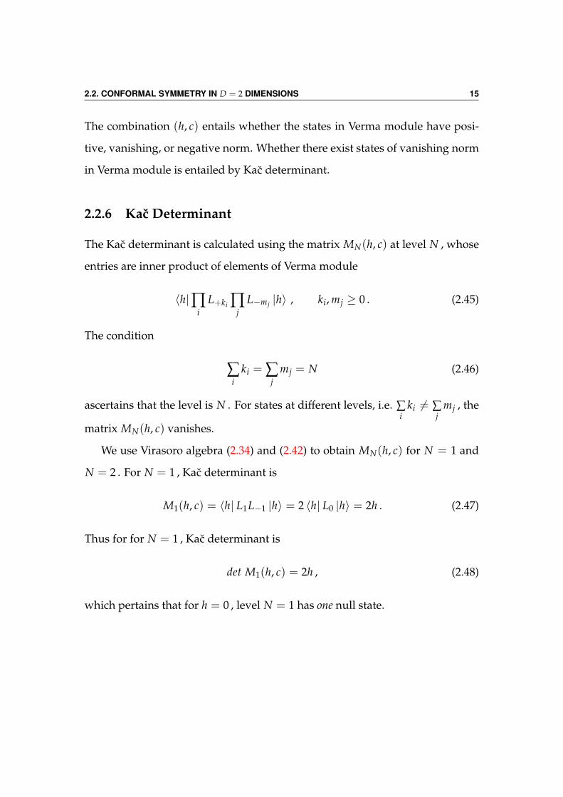
The combination (h, c) entails whether the states in Verma module have posi-
tive, vanishing, or negative norm. Whether there exist states of vanishing norm
in Verma module is entailed by Kac determinant.
2.2.6 Kac Determinant
The Kac determinant is calculated using the matrix MN(h, c) at level N , whose
entries are inner product of elements of Verma module
〈h|∏i
L+ki ∏j
L−mj |h〉 , ki, mj ≥ 0 . (2.45)
The condition
∑i
ki = ∑j
mj = N (2.46)
ascertains that the level is N . For states at different levels, i.e. ∑i
ki 6= ∑j
mj , the
matrix MN(h, c) vanishes.
We use Virasoro algebra (2.34) and (2.42) to obtain MN(h, c) for N = 1 and
N = 2 . For N = 1 , Kac determinant is
M1(h, c) = 〈h| L1L−1 |h〉 = 2 〈h| L0 |h〉 = 2h . (2.47)
Thus for for N = 1 , Kac determinant is
det M1(h, c) = 2h , (2.48)
which pertains that for h = 0 , level N = 1 has one null state.
2.2. CONFORMAL SYMMETRY IN D = 2 DIMENSIONS 16
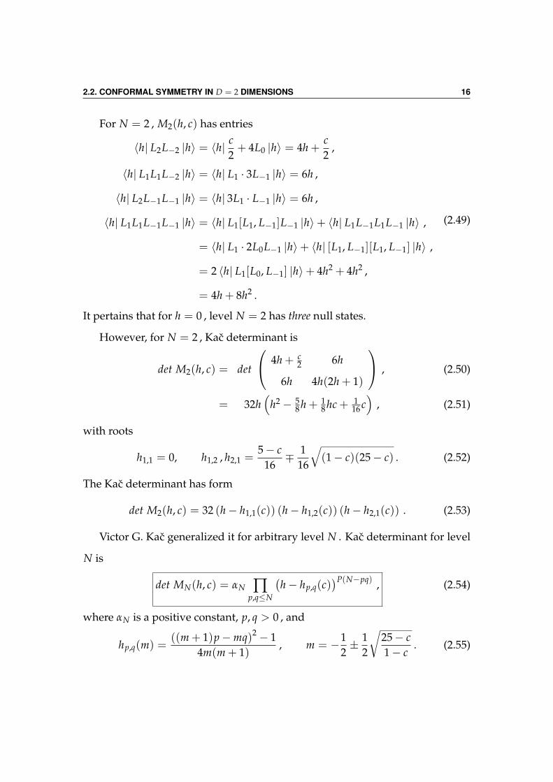
For N = 2 , M2(h, c) has entries
〈h| L2L−2 |h〉 = 〈h|c2+ 4L0 |h〉 = 4h +
c2
,
〈h| L1L1L−2 |h〉 = 〈h| L1 · 3L−1 |h〉 = 6h ,
〈h| L2L−1L−1 |h〉 = 〈h| 3L1 · L−1 |h〉 = 6h ,
〈h| L1L1L−1L−1 |h〉 = 〈h| L1[L1, L−1]L−1 |h〉+ 〈h| L1L−1L1L−1 |h〉 ,
= 〈h| L1 · 2L0L−1 |h〉+ 〈h| [L1, L−1][L1, L−1] |h〉 ,
= 2 〈h| L1[L0, L−1] |h〉+ 4h2 + 4h2 ,
= 4h + 8h2 .
(2.49)
It pertains that for h = 0 , level N = 2 has three null states.
However, for N = 2 , Kac determinant is
det M2(h, c) = det
4h + c2 6h
6h 4h(2h + 1)
, (2.50)
= 32h(
h2 − 58 h + 1
8 hc + 116 c)
, (2.51)
with roots
h1,1 = 0, h1,2 , h2,1 =5− c
16∓ 1
16
√(1− c)(25− c) . (2.52)
The Kac determinant has form
det M2(h, c) = 32 (h− h1,1(c)) (h− h1,2(c)) (h− h2,1(c)) . (2.53)
Victor G. Kac generalized it for arbitrary level N . Kac determinant for level
N is
det MN(h, c) = αN ∏p,q≤N
(h− hp,q(c)
)P(N−pq) , (2.54)
where αN is a positive constant, p, q > 0 , and
hp,q(m) =((m + 1)p−mq)2 − 1
4m(m + 1), m = −1
2± 1
2
√25− c1− c
. (2.55)
Chapter3Superconformal Symmetry
3.1 Suppersymmetry
Suppersymmetry has its roots in work of Miyazawa (1966) [21]. Suppersym-
metry unifies matter with mediators, and statistics of bosonic and fermionic
sectors1.
Supersymmetry reduces bosonfermion and interactionmatter hier-
archies (diads), and simplifies them to susyon and supersystem (monads).
bosonfermion is compositional containment hierarchy; fermions constitute
bosons, but not conversely.
Bosonic and fermionic sectors of QFTs entail (ultraviolet) divergences. Sup-
persymmetry entails fermions and bosons on equal footing, that cancels these
infinities via pairing-off divergences of superpartners. Supersymmetry is a
semi-finitistic prescription [25]. A more radical finitistic prescription is met in
1Provisionally, 1024 bosons collectively behave as fermions in Palev statistics [24]; Palev sets
an upper bound (provisionally 1024) to the degeneracy of bosons from algebraic regularization
scheme. How do supersymmetric models entail palevons?
17
3.1. SUPPERSYMMETRY 18
string models, which entail supersymmetry as well as extra-dimensions. Nev-
ertheless, supersymmetry appears to be symptom of finitism for quantum field
theories, which remains sole motivation for making QFTs suppersymmetric.
The generators of suppersymmetry Qr ∈ QS , also termed supercharges, trans-
form bosons (systems with integral-spin 0, 1, 2, . . . ) into fermions (systems with
half-integral-spin 1/2, 3/2, 5/2, . . . ), and vice versa
Qr |boson〉 = | f ermion〉 , Qr | f ermion〉 = |boson〉 . (3.1)
Particles so related by (3.1) are termed superpartners. It is customary to suffix
fermionic superpartners of bosons with -ino, and prefix bosonic superpartners
of fermions with s-. It is anticipated that every fundamental particle found in
nature has a superpartner. Superpartner of electron would be spin-0 selectron,
and superpartner of photon would be spin-1/2 photino.
The generators concerned here are operators in Hilbert space, that annihilate
a particle, and create another one in the state space of the system-under-study,
leaving physics intact. The generator has a general form [29],
G = ∑ij
∫d3pd3q a†
i (p)Kij(q, p)aj(q) , (3.2)
which has symbolic form as convolutions,
G = a† ∗ K ∗ a . (3.3)
The operator G is termed generator of a symmetry if it commutes with the
S-matrix
[S, G] = 0 , (3.4)
which leaves the physics invariant under transformations of G on system-under-
study. The symmetry generator G is decomposed into bosonic (even) and fermionic
3.1. SUPPERSYMMETRY 19
(odd) parts
G = B + F . (3.5)
B transforms bosons-to-bosons and fermions-to-fermions, while F transforms
bosons-to-fermions and vice-versa. For bosonic and fermionic creators b†, f † and
annihilators b, f , B and F entail representations
B = b† ∗ Kbb ∗ b + f † ∗ K f f ∗ f ,
F = f † ∗ K f b ∗ b + b† ∗ Kb f ∗ f .(3.6)
Acting on a state |j〉 ,
B |j〉 = |j± n〉 , F |j〉 = |j± n/2〉 , ∀ n ∈ Z∗ . (3.7)
Thus fermionic generators F (3.6) are essentially supersymmetric ones (3.1).
Virasoro algebra (2.34) holds for both bosonic and fermionic sectors, which are
autonomous to each other. However, in the sense of (3.5), Virasoro generators
Ln decompose into bosonic and fermionic ones,
Ln := Lbos.n + L f erm.
n , (3.8)
where, Lbos.n and L f erm.
n separately satisfy Virasoro algebra (2.34), with central
charges c = 1 and c = 1/2 , while Ln (3.8) satisfies Virasoro algebra with central
charge c = 3/2 . The bosonic and fermionic Virasoro generators satisfy
[Lbos.m , L f erm.
n ] = 0 . (3.9)
In field-theoretic-regime [6], energy-momentum tensor T(z) has Laurent ex-
pansion
T(z) = ∑n∈Z
Lnz−n−2 , Ln =1
2πi
∮dz zn+1T(z) , (3.10)
3.2. SUPERSPACE 20
having fermionic superpartner G(z) , with Laurent expansion
G(z) = ∑r∈Z+ 1
2
Grz−r− 32 , Gr = ∑
s∈Z+ 12
jr−sψs , (3.11)
where, j(z) and ψ(z) are primary fields (2.38) of conformal dimensions h = 1 ,
and h = 1/2 , having Laurent expansions
j(z) = ∑n∈Z
jnz−n−1 ,
ψ(z) = ∑r
ψrz−r− 12 ,
(3.12)
However, G(z) (3.11) is a fermionic field, constructed from bosonic field j(z) and
fermionic field ψ(z) .
3.2 Superspace
The superspace is 2-dimensional vector space (analogous to C) with basis Z =
(z, Θ) , where z ∈ C , and Θ (analogous to i) is Grassmann variable satisfying
Θ, Θ = 0 , (3.13)
implying Θ2 = 0 . The derivative acting on a superfield Φ(Z) parametrized by
Z is defined as
D := ∂Θ + Θ∂z , (3.14)
with D2 = ∂z . The superfield Φ(Z) has bosonic and fermionic components φ(z)
and ψ(z) , with
Φ(Z) = φ(z) + Θψ(z) . (3.15)
3.3. N = 1 SUPER VIRASORO ALGEBRA 21
3.3 N = 1 Super Virasoro Algebra
Minimal supersymmetry (N = 1) entails one superpartner to each system (par-
ticle or field). The super Virasoro generators Ln, Lm ∈ LV , and Gr, Gs ∈ GS
satisfy commutation relations
[Lm, Ln] = (m− n)Lm+n +c
12(m3 −m)δm+n,0 ,
[Lm, Gr] =(m
2− r)
Gm+r ,
Gr, Gs = 2Lr+s +c3
(r2 − 1
4
)δr+s,0 ,
(3.16)
which form infinite dimensional Lie algebra, termed N = 1 Super Virasoro Alge-
bra SVAN=1(LV ,GS) .
3.4 Highest Weight Representations ofN = 1 Super
Virasoro Algebra
The state |h〉 satisfying
Ln |h〉 = 0 , for n > 0 , (3.17)
Gr |h〉 = 0 , for r > 0 , (3.18)
is termed superconformal highest weight state. However, for 0 < c < 3/2 , unitary
highest weight representations of super Virasoro algebra entail discrete values
of central charge,
c =32
(1− 8
(m + 2)(m + 4)
), m ∈ Z . (3.19)
3.5. N = 2 SUPER VIRASORO ALGEBRA 22
3.5 N = 2 Super Virasoro Algebra
N = 2 supersymmetric models entail two superpartners to each system (particle
or field). We define complex free bosonic field
Φ(z, z) =1√2
(X(1)(z, z) + i X(2)(z, z)
). (3.20)
However, free boson X(z, z) has vanishing conformal dimension, and thus, is
not a conformal field. Instead, j(z) = i∂X(z, z) , or Vertex operator V(z, z) =:
eiαX(z,z) : is used as conformal free bosonic field [6]. Thus, we have complex free
bosonic and fermionic fields
j(z) =1√2
(j(1)(z) + i j(2)(z)
),
Ψ(z) =1√2
(Ψ(1)(z) + i Ψ(2)(z)
).
(3.21)
The Laurent modes of bosonic current j(z) are
jn = −i ∑s∈Z+ 1
2
ψ(1)n−sψ
(2)s , (3.22)
In analogy to N = 1 case (3.11), we construct a fermionic field G(z) having
bosonic and fermionic contributions, which, for N = 2 has two parts G+(z)
and G−(z) ,
G(z) = G+(z) + G−(z) =1√2
(G(1)(z) + G(2)(z)
), (3.23)
having Laurent modes,
G±r =1√2
∑s∈Z+ 1
2
(j(1)r−s ∓ i j(2)r−s
) (ψ(1)s ± i ψ
(2)s
), (3.24)
Unlike N = 1 , here we have two generators for each bosonic and fermionic
field. Thus, the Laurent mode (3.8) for N = 2 satisfies Virasoro algebra (2.34)
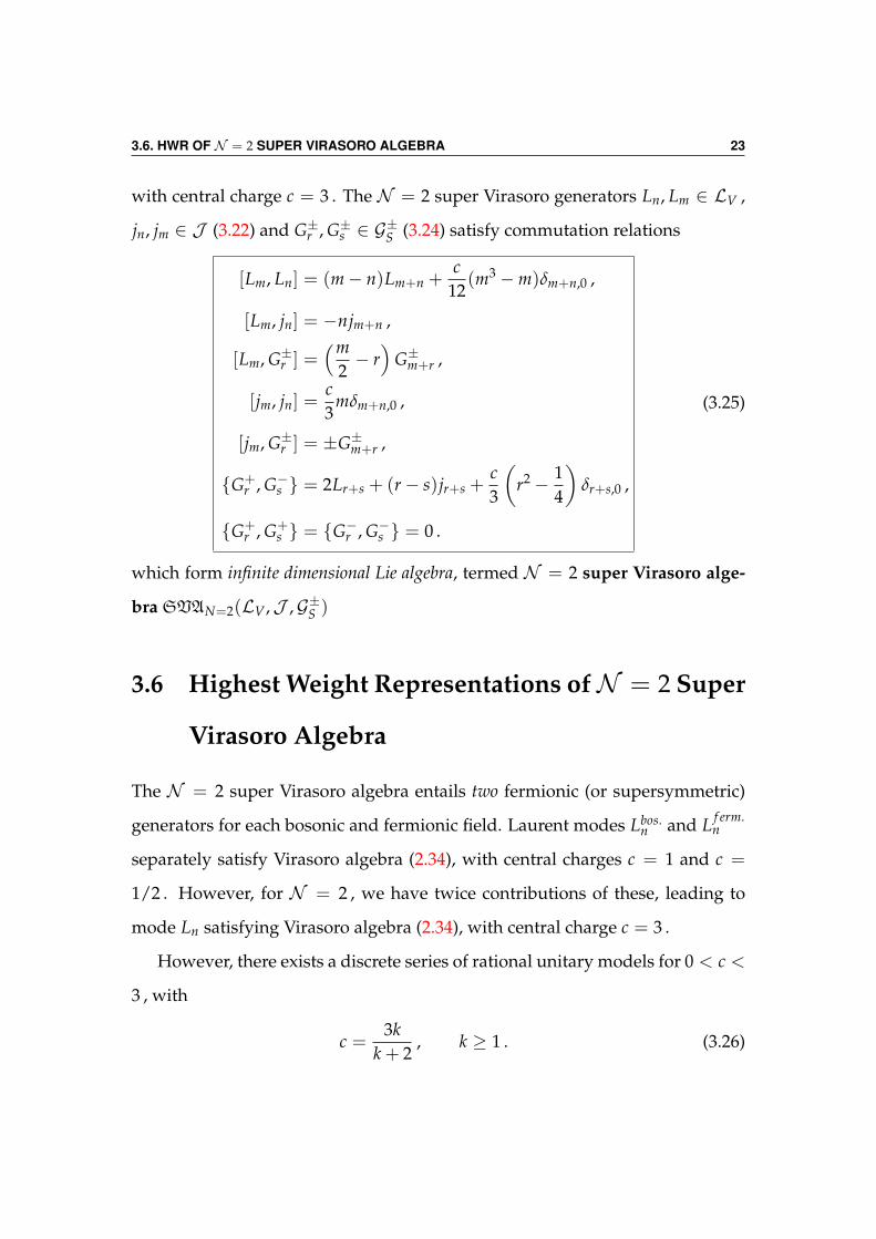
3.6. HWR OF N = 2 SUPER VIRASORO ALGEBRA 23
with central charge c = 3 . The N = 2 super Virasoro generators Ln, Lm ∈ LV ,
jn, jm ∈ J (3.22) and G±r , G±s ∈ G±S (3.24) satisfy commutation relations
[Lm, Ln] = (m− n)Lm+n +c
12(m3 −m)δm+n,0 ,
[Lm, jn] = −njm+n ,
[Lm, G±r ] =(m
2− r)
G±m+r ,
[jm, jn] =c3
mδm+n,0 ,
[jm, G±r ] = ±G±m+r ,
G+r , G−s = 2Lr+s + (r− s)jr+s +
c3
(r2 − 1
4
)δr+s,0 ,
G+r , G+
s = G−r , G−s = 0 .
(3.25)
which form infinite dimensional Lie algebra, termed N = 2 super Virasoro alge-
bra SVAN=2(LV ,J ,G±S )
3.6 Highest Weight Representations ofN = 2 Super
Virasoro Algebra
The N = 2 super Virasoro algebra entails two fermionic (or supersymmetric)
generators for each bosonic and fermionic field. Laurent modes Lbos.n and L f erm.
n
separately satisfy Virasoro algebra (2.34), with central charges c = 1 and c =
1/2 . However, for N = 2 , we have twice contributions of these, leading to
mode Ln satisfying Virasoro algebra (2.34), with central charge c = 3 .
However, there exists a discrete series of rational unitary models for 0 < c <
3 , with
c =3k
k + 2, k ≥ 1 . (3.26)
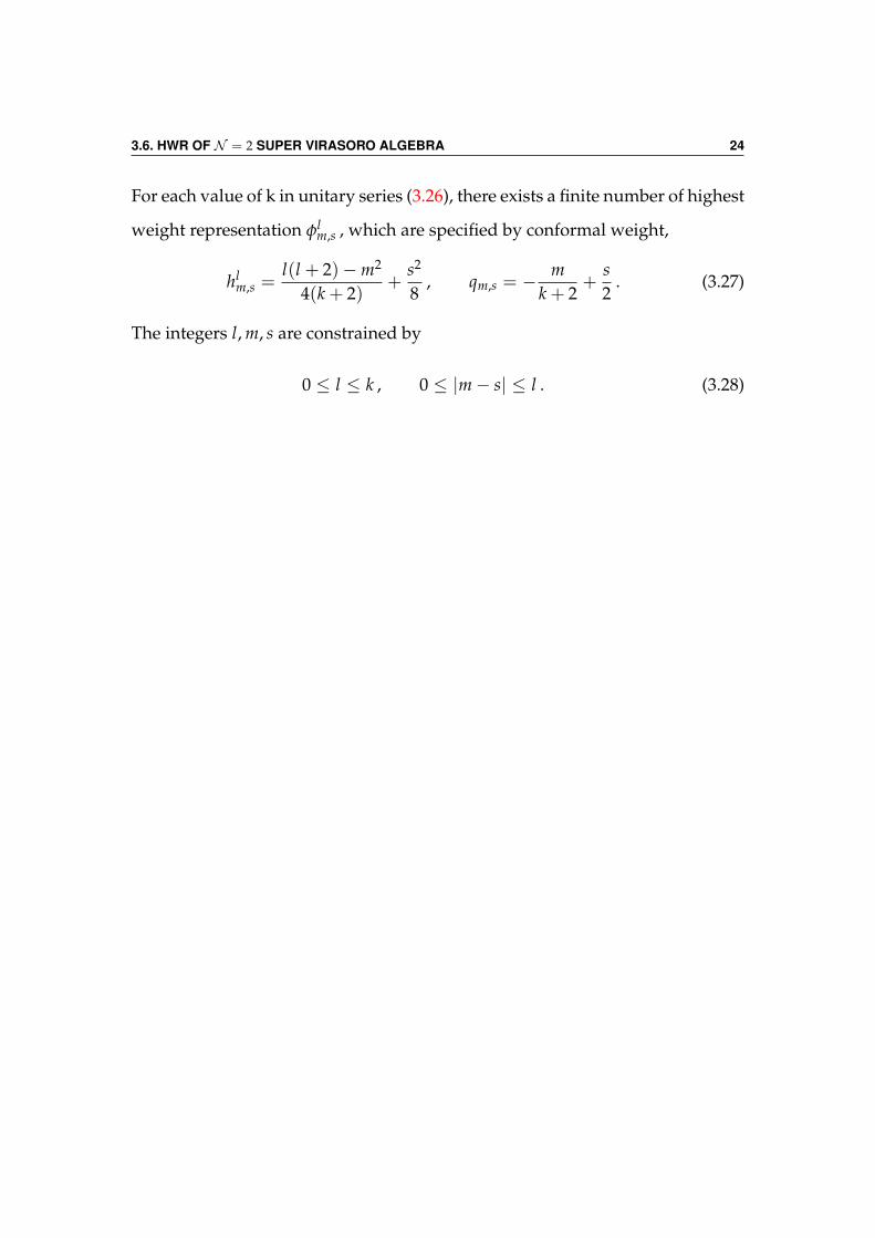
3.6. HWR OF N = 2 SUPER VIRASORO ALGEBRA 24
For each value of k in unitary series (3.26), there exists a finite number of highest
weight representation φlm,s , which are specified by conformal weight,
hlm,s =
l(l + 2)−m2
4(k + 2)+
s2
8, qm,s = −
mk + 2
+s2
. (3.27)
The integers l, m, s are constrained by
0 ≤ l ≤ k , 0 ≤ |m− s| ≤ l . (3.28)
Chapter4Summary
This report summarizes algebraic aspects of conformal symmetry, suppersym-
metry, superconformal symmetry, and their corresponding algebras. In the In-
troduction, I defined infinitesimal symmetry, and constructed the notion of gen-
erator of symmetry. I formalized infinitesimal symmetry and finite continuous
symmetry, and discussed their relevance in physics.
In chapter 2, I introduced conformal symmetry in d-dimensions, and devel-
oped conformal symmetry in 2-dimensions. Section 2.1 summarizes conformal
algebra in d-dimensions. Section 2.2 summarizes Witt algebra and its central
extension, called Virasoro algebra, and its highest weight representations. The
highest weight representation of Virasoro algebra entails Verma module. Verma
module has states with vanishing norm, which were ascertained using Kac de-
terminant. Section 2.2.6 summarizes Kac determinant for levels N = 1 and
N = 2 , and it was further generalized for arbitrary level N .
Chapter 3 introduces suppersymmetry and supperconformal symmetry, and
summarizes super Virasoro algebra for N = 1 and N = 2 , and their highest
weight representations.
25
Bibliography
[1] Ian Aitchison. Supersymmetry in Particle Physics. Cambridge University
Press, Cambridge, 2007.
[2] A.O. Barut et. al. Conformal Groups and Related Symmetries. Lecture Notes
in Physics. Springer, Berlin, 1986.
[3] Marco Baumgartl et. al. Strings and Fundamental Physics. Lecture Notes in
Physics. Springer, Berlin, 2012.
[4] F. Bayen, M. Flato, C. Frønsdal, A. Lichnerowicz, and D. Sternheimer. De-
formation theory and quantization i.& ii. Annals of Physics, 111(1):61–151,
1978.
[5] K. Becker, M. Becker, and J.H. Schwarz. String Theory and M-Theory. Cam-
bridge University Press, Cambridge, 2007.
[6] R. Blumenhagen and E. Plauschinn. Introduction to Conformal Field Theory.
Lecture Notes in Physics. Springer, Berlin, 2009.
[7] Ralph Blumenhagen, Dieter Lust, and Stefan Theisen. Basic Concepts of
String Theory. Theoretical and Mathematical Physics. Springer, Berlin, 2013.
26
BIBLIOGRAPHY 27
[8] Giovanni Costa and Gianluigi Fogli. Symmetries and Group Theory in Particle
Physics. Lecture Notes in Physics. Springer, Berlin, 2012.
[9] Peter G.O. Freund. Introduction to Supersymmetry. Cambridge Monographs
on Mathematical Physics. Cambridge University Press, Cambridge, 1986.
[10] Y. Frishman and J. Sonnenschein. Non-Perturbative Field Theory: From Two-
Dimensional Conformal Field Theory to QCD in Four Dimensions. Cambridge
Monographs on Mathematical Physics. Cambridge University Press, Cam-
bridge, 2010.
[11] Jurgen Fuchs and Christoph Schweigert. Symmetries, Lie Algebras and Rep-
resentations. Cambridge University Press, Cambridge, 1997.
[12] M. Gasperini and J. Maharana. String Theory and Fundamental Interactions.
Lecture Notes in Physics. Springer, Berlin, 2008.
[13] Paul Ginsparg. Applied conformal field theory. 1988. arXiv: hep-
th/9108028.
[14] M.B. Green, J.H. Schwarz, and E. Witten. Superstring Theory Vol. I.
Cambridge Monographs on Mathematical Physics. Cambridge University
Press, Cambridge, 1987.
[15] M.B. Green, J.H. Schwarz, and E. Witten. Superstring Theory Vol. II.
Cambridge Monographs on Mathematical Physics. Cambridge University
Press, Cambridge, 1987.
[16] Malte Henkel. Conformal Invariance and Critical Phenomena. Theoretical and
Mathematical Physics. Springer, Berlin, 1999.
BIBLIOGRAPHY 28
[17] W. Hollik et. al. Phenomenological Aspects of Supersymmetry. Lecture Notes
in Physics. Springer, Berlin, 1992.
[18] Hajime Ishimori et. al. An Introduction to Non-Abelian Discrete Symmetries
for Particle Physicists. Lecture Notes in Physics. Springer, Berlin, 2012.
[19] Clifford V. Johnson. D-Branes. Cambridge Monographs on Mathematical
Physics. Cambridge University Press, Cambridge, 2003.
[20] A. Kapustin et. al. Homological Mirror Symmetry. Lecture Notes in Physics.
Springer, Berlin, 2009.
[21] H. Miyazawa. Baryon Number Changing Currents. Progress of Theoretical
Physics, 36(6), 1966.
[22] H. Miyazawa. Superalgebra and Fermion-Boson Symmetry. Proc. Jpn.
Acad., Ser. B, 86, 2010.
[23] Tomas Ortin. Gravity and Strings. Cambridge Monographs on Mathemati-
cal Physics. Cambridge University Press, Cambridge, 2004.
[24] T.D. Palev. Lie Algebraical Aspects of the Quantum Statistics. Uni-
tary Quantization (A-quantization). JINR E17-10550, 1977. arXiv: hep-
th/9705032.
[25] Roger Penrose. The Road to Reality. Jonathan Cape, London, 2004.
[26] Joseph Polchinski. String Theory Vol. I. Cambridge Monographs on Math-
ematical Physics. Cambridge University Press, Cambridge, 2001.
[27] Joseph Polchinski. String Theory Vol. II. Cambridge Monographs on Math-
ematical Physics. Cambridge University Press, Cambridge, 2005.
[28] M. Schottenloher. A Mathematical Introduction to Conformal Field Theory. Lec-
ture Notes in Physics. Springer, Berlin, 2008.
[29] M.F. Sohnius. Introducing supersymmetry. Physics Reports, 128(2 & 3):39–
204, 1985.
[30] V.S. Varadarajan. Supersymmetry for Mathematicians. Courant Lecture
Notes. American Mathematical Society, 2004.
[31] V.S. Varadarajan et. al. A Mathematical Introduction to Conformal Field Theory.
Lecture Notes in Mathematics. Springer, Berlin, 2010.
[32] S. Weinberg. Quantum Theory of Fields III: Supersymmetry. Cambridge Uni-
versity Press, Cambridge, 2000.
[33] J. Wess. Supersymmetry and Supergravity. Princeton Series in Physics.
Princeton University Press, Princeton, 1992.
[34] J. Wess and E. Ivanov. Supersymmetries and Quantum Symmetries. Lecture
Notes in Physics. Springer, Berlin, 1999.
[35] Hermann Weyl. The Theory of Groups and Quantum Mechanics. Dover Pub-
lications, New York, 1931.
[36] Barton Zwiebach. A First Course in String Theory. Cambridge University
Press, Cambridge, 2009.
Recommended