University of Illinois at Urbana-Champaign
Air Conditioning and Refrigeration Center A National Science Foundation/University Cooperative Research Center
Condensation of Ammonia in Microchannel Heat Exchangers
A. D. Litch and P. S. Hrnjak
ACRC CR-22 August 1999
For additional information: Air Conditioning and Refrigeration Center University of Illinois Mechanical & Industrial Engineering Dept. 1206 West Green Street Urbana, IL 61801 (217) 333-3115

The Air Conditioning and Refrigeration Center was founded in 1988 with a grant from the estate of Richard W. Kritzer, the founder of Peerless of America Inc. A State of Illinois Technology Challenge Grant helped build the laboratory facilities. The ACRC receives continuing support from the Richard W. Kritzer Endowment and the National Science Foundation. The following organizations have also become sponsors of the Center. Amana Refrigeration, Inc. Brazeway, Inc. Carrier Corporation Caterpillar, Inc. Chrysler Corporation Copeland Corporation Delphi Harrison Thermal Systems Frigidaire Company General Electric Company Hill PHOENIX Honeywell, Inc. Hussmann Corporation Hydro Aluminum Adrian, Inc. Indiana Tube Corporation Lennox International, Inc. Modine Manufacturing Co. Peerless of America, Inc. The Trane Company Thermo King Corporation Visteon Automotive Systems Whirlpool Corporation York International, Inc. For additional information: Air Conditioning & Refrigeration Center Mechanical & Industrial Engineering Dept. University of Illinois 1206 West Green Street Urbana, IL 61801 217 333 3115
iii
Table of Contents
Page
List of Figures ............................................................................................................................. v
List of Tables ............................................................................................................................ viii
Nomenclature............................................................................................................................. ix
Chapter 1: Introduction ............................................................................................................ 1
1.1 Background...........................................................................................................................1
1.2 Objective ...............................................................................................................................1
Chapter 2: Experimental Facility............................................................................................ 3
2.1 Wind Tunnel Design ..............................................................................................................3
2.2 Ammonia Chiller Setup .........................................................................................................6
2.3 Glycol Heat Recovery Loop...................................................................................................7
2.4 Condenser Test Specimens ..................................................................................................7
2.5 Experimental Uncertainty.................................................................................................... 10
Chapter 3: Simulation Description ......................................................................................13
3.1 Coil Discretization............................................................................................................... 13
3.2 Modeling Equations ............................................................................................................ 14
3.2.1 Heat Transfer.........................................................................................................................................................14 3.2.2 Pressure Drop ........................................................................................................................................................18 3.2.3 Refrigerant Inventory...........................................................................................................................................21 3.2.4 Header Modeling ..................................................................................................................................................22
Chapter 4: Results & Discussion.........................................................................................26
4.1 Serpentine Condenser ........................................................................................................ 26
4.1.1 Overall Heat Transfer Performance...................................................................................................................26 4.1.2 Air Side Heat Transfer.........................................................................................................................................27 4.1.3 Air Side Pressure Drop ........................................................................................................................................29 4.1.4 Predicted Heat Transfer.......................................................................................................................................30 4.1.5 Refrigerant Pressure Drop...................................................................................................................................31 4.1.6 Refrigerant Inventory...........................................................................................................................................32
4.2 Microchannel Condenser .................................................................................................... 34
4.2.1 Overall Heat Transfer Performance...................................................................................................................34 4.2.2 Air Side Heat Transfer.........................................................................................................................................35 4.2.3 Air Side Pressure Drop ........................................................................................................................................36
iv
4.2.4 Predicted Heat Transfer.......................................................................................................................................38 4.2.5 Refrigerant Pressure Drop...................................................................................................................................41 4.2.6 Refrigerant Inventory...........................................................................................................................................42
4.3 Refrigerant Distribution....................................................................................................... 43
4.3.1 Air Exit Temperature Distribution.....................................................................................................................43 4.3.2 Infrared Camera Sensing of Tube Surface Temperature ................................................................................44 4.3.3 Single Tube Model Second Pass Output...........................................................................................................47
4.4 Condenser Comparison ...................................................................................................... 49
4.5 Microchannel Optimization for Ammonia............................................................................ 49
4.6 System Comparison ............................................................................................................ 51
Chapter 5: Conclusions and Recommendations.............................................................53
5.1 Summary and Conclusions................................................................................................. 53
5.2 Recommendations.............................................................................................................. 53
Appendix A: Test Data ............................................................................................................55
Appendix B: Local Temperature Distribution...................................................................57
Appendix C: Wilson Plot Analysis .......................................................................................73
Appendix D: Simulation Code ..............................................................................................75
Appendix E: Experimental Setup Components ...............................................................91
Evaporator:............................................................................................................................... 95
List of References ....................................................................................................................96
v
List of Figures
Page
Figure 1.1: Refrigerant Saturation Temperature Loss with Pressure Drop.............................................................................1 Figure 2.1: Ammonia Test Facility Schematic ............................................................................................................................4 Figure 2.2: Horizontal Velocity Profile at Test Section Inlet, 0.6 m3/sec average flow rate...............................................5 Figure 2.3: Horizontal Velocity Profile at Test Section Inlet, 1.1 m3/sec average flow rate...............................................5 Figure 2.4: Serpentine Condenser Schematic ..............................................................................................................................8 Figure 2.5: Microchannel Condenser Schematic .........................................................................................................................9 Figure 2.6: Propagation of Uncertainty in Serpentine Condenser Heat Transfer Measurements .....................................11 Figure 2.7: Propagation of Uncertainty in Microchannel Condenser Heat Transfer Measurements ...............................11 Figure 3.1: Microchannel Condenser Module Distribution Among Header Sections and Passes ....................................14 Figure 3.2: Header Section Two Module....................................................................................................................................22 Figure 4.1: Serpentine Condenser Heat Balance.......................................................................................................................26 Figure 4.2: Overall Heat Transfer Coefficients in Serpentine Condenser Based on Air Side Surface Area ..................27 Figure 4.3: Existing Multi-louver Heat Transfer Correlations Applied to Serpentine Condenser...................................28 Figure 4.4: Serpentine Condenser Air Side Heat Transfer Results........................................................................................29 Figure 4.5: Serpentine Air Pressure Drop Compared to Existing Multi-louver Pressure Drop Correlations.................29 Figure 4.6: Serpentine Condenser Predicted Heat Transfer Using Dobson’s Annular Prediction ...................................30 Figure 4.7: Predicted and Measured Ammonia Temperatures Along Serpentine Condenser Tube, Data Point 5 ........31 Figure 4.8: Serpentine Condenser Local Refrigerant Heat Transfer Coefficients for Data Point 4.................................31 Figure 4.9: Serpentine Condenser Ammonia Pressure Drop...................................................................................................32 Figure 4.10: Serpentine Condenser Total Charge .....................................................................................................................33 Figure 4.11: Predicted Local Distribution of Mass, Newell Void Fraction, Serpentine Data Point 1 .............................34 Figure 4.12: Microchannel Condenser Heat Balance ...............................................................................................................34 Figure 4.13: Overall Heat Transfer Coefficients in Microchannel Condenser Based on Air Side Surface Area ..........35 Figure 4.14: Existing Multi-louver Heat Transfer Correlations Applied to Microchannel Condenser...........................35 Figure 4.15: Experimental and Predicted Results for Microchannel Air Heat Transfer Coefficients..............................36 Figure 4.16: Microchannel Air Pressure Drop Compared to Existing Multi-louver Pressure Drop Correlations.........37 Figure 4.17: Experimental Airside Pressure Drop Comparison Between Condensers .......................................................37 Figure 4.18: Microchannel Condenser Predicted Heat Transfer, Single Tube Model........................................................38 Figure 4.19: Microchannel Condenser Local Refrigerant Heat Transfer Coefficients for Data Point 3 .........................39 Figure 4.20: Microchannel Condenser Predicted Heat Transfer, Uniform Model ..............................................................40 Figure 4.21: Predictions for Microchannel Second Pass Heat Transfer in Single Tube and Uniform Models ..............40 Figure 4.22: Microchannel Condenser Ammonia Pressure Drop with Comparison to Model Prediction ......................41 Figure 4.23: Microchannel Ammonia Pressure Drop Dependence on Mass Flux..............................................................41 Figure 4.24: Microchannel Condenser Total Charge Measurements with Model Comparison........................................42 Figure 4.25: Predicted Local Contribution of Mass, Microchannel Data Point 1 ...............................................................43 Figure 4.26: Microchannel Condenser Contoured Air Exit Temperatures (°C), Data Point 8..........................................44 Figure 4.27: Infrared Camera Target Area on Microchannel Condenser..............................................................................45
vi
Figure 4.28: Infrared Camera Contour of Target Area with Corresponding Air Outlet Temperature Contour;
Conditions Correspond to Microchannel Data Point 12 .................................................................................................46 Figure 4.29: Linear Temperature Profiles at Bottom Edge of IR Camera Target Area......................................................47 Figure 4.30: 2nd Pass Single Tube Predicted Air Exit Temperatures and Ammonia Qualities, Data Point 6 ...............48 Figure 4.31: Heat Transfer and Pressure Dependence on Number of Microchannel Condenser Tubes .........................50 Figure 4.32: Mass Flux Dependence on Number of Tubes .....................................................................................................51 Figure 4.33: Predicted 13 Tube Heat Transfer...........................................................................................................................51 Figure B.1: Serpentine Model Refrigerant Temperatures Compared to Surface Thermocouples, Data Point 1............57 Figure B.2: Serpentine Model Refrigerant Temperatures Compared to Surface Thermocouples, Data Point 2............57 Figure B.3: Serpentine Model Refrigerant Temperatures Compared to Surface Thermocouples, Data Point 3............58 Figure B.4: Serpentine Model Refrigerant Temperatures Compared to Surface Thermocouples, Data Point 4............58 Figure B.5: Serpentine Model Refrigerant Temperatures Compared to Surface Thermocouples, Data Point 5............59 Figure B.6: Serpentine Model Refrigerant Temperatures Compared to Surface Thermocouples, Data Point 6............59 Figure B.7: Serpentine Model Refrigerant Temperatures Compared to Surface Thermocouples, Data Point 7............60 Figure B.8: Serpentine Model Refrigerant Temperatures Compared to Surface Thermocouples, Data Point 8............60 Figure B.9: Microchannel Air Exit Temperatures (°C) from Thermocouple Grid, Data Point 1.....................................61 Figure B.10: Microchannel Air Exit Temperatures (°C) from Thermocouple Grid, Data Point 2 ...................................61 Figure B.11: Microchannel Air Exit Temperatures (°C) from Thermocouple Grid, Data Point 3 ...................................62 Figure B.12: Microchannel Air Exit Temperatures (°C) fro m Thermocouple Grid, Data Point 4 ...................................62 Figure B.13: Microchannel Air Exit Temperatures (°C) from Thermocouple Grid, Data Point 5 ...................................63 Figure B.14: Microchannel Air Exit Temperatures (°C) from Thermocouple Grid, Data Point 6 ...................................63 Figure B.15: Microchannel Air Exit Temperatures (°C) from Thermocouple Grid, Data Point 7 ...................................64 Figure B.16: Microchannel Air Exit Temperatures (°C) from Thermocouple Grid, Data Point 8 ...................................64 Figure B.17: Microchannel Air Exit Temperatures (°C) from Thermocouple Grid, Data Point 9 ...................................65 Figure B.18: Microchannel Air Exit Temperatures (°C) from Thermocouple Grid, Data Point 10.................................65 Figure B.19: Microchannel Air Exit Temperatures (°C) from Thermocouple Grid, Data Point 11.................................66 Figure B.20: Microchannel Air Exit Temperatures (°C) from Thermocouple Grid, Data Point 12.................................66 Figure B.21: Microchannel Air Exit Temperatures (°C) from Thermocouple Grid, Data Point 13.................................67 Figure B.22: Microchannel Air Exit Temperatures (°C) from Thermocouple Grid, Data Point 14.................................67 Figure B.23: Microchannel Air Exit Temperatures (°C) from Thermocouple Grid, Data Point 15.................................68 Figure B.24: Microchannel Air Exit Temperatures (°C) from Thermocouple Grid, Data Point 16.................................68 Figure B.25: Microchannel Air Exit Temperatures (°C) from Thermocouple Grid, Data Point 17.................................69 Figure B.26: Predicted Second Pass Parameter Comparison for Header Section Inlet Quality 1.0, Data Point 6.........70 Figure B.27: Predicted Second Pass Parameter Comparison for Header Section Inlet Quality 0.8, Data Point 6.........71 Figure B.28: Predicted Second Pass Parameter Comparison for Header Section Inlet Quality 0.6, Data Point 6.........72 Figure C.1: Typical Wilson Plot ..................................................................................................................................................73 Figure C.2: Wilson Plots for Serpentine Condenser at Multiple Air Flow Rates................................................................74 Figure E.1: Serpentine Condenser...............................................................................................................................................91 Figure E.2: Microchannel Condenser with Air Exit Thermocouple Grid .............................................................................91 Figure E.3: Wind Tunnel...............................................................................................................................................................92

vii
Figure E.4: Wind Tunnel and Chiller Test Bed.........................................................................................................................93 Figure E.5: Wind Tunnel and Chiller Test Bed, Alternate View...........................................................................................94 Figure E.6: Chiller Test Bed Components..................................................................................................................................95
viii
List of Tables
Page
Table 2.1: Condenser Comparison of Physical Parameters .......................................................................................................7 Table 2.2: Uncertainty of Individual Measurements ................................................................................................................10 Table 3.1: Hughmark Correlating Parameter and Inverse Slip Relationship .......................................................................23 Table 4.1: Comparison Parameters for Ammonia Condensers ...............................................................................................49 Table 4.2: Ammonia Chiller Charge Comparison ....................................................................................................................52 Table A.1: Serpentine Condenser Experimental Data..............................................................................................................55 Table A.2: Microchannel Condenser Experimental Data ........................................................................................................56
ix
Nomenclature
Roman and Script Letters a = exponent in quality distribution
A = area term in Churchill’s friction factor equation
B = term in Churchill’s friction factor equation
c = constant in two-phase flow multiplier equations
C = slope constant in Wilson Plot analysis
cp = constant pressure specific heat
Cr = heat capacity rate ratio
D = diameter
Dp = depth
f = friction factor
Fr = Froude number, ratio of gravitational forces to inertial effects
Ft = Froude rate, ratio of vapor flow’s power to power required to pump liquid
from the bottom to the top of a tube
g = gravitational acceleration
G = mass flux
Ga = Galileo number, ratio of gravitational forces to viscous forces
h = heat transfer coefficient
H = height
i = enthalpy
j = St Pr2/ , Colburn factor
Ja = Jakob number, ratio of sensible energy transfer to latent energy transfer
k = thermal conductivity
K = loss coefficient
inverse slip ratio defined by Hughmark
L = length
m = mass of refrigerant
M = material mass of heat exchanger
n = node number
NTU = heat exchanger number of transfer units
Nu = hDk
, Nusslet number
P = pressure pitch
Pr = µck
p, Prandtl number
&Q = heat transfer rate
R = thermal resistance

x
Re = Reynolds number
S = slip ratio, vapor velocity to liquid velocity
St = h
cpρ V, Stanton number
t = thickness
T = temperature
U = overall heat transfer coefficient
UA = overall heat exchanger thermal conductance
v = specific volume
V = volume V = velocity
w = mass flow rate
x = thermodynamic quality
y = vertical distance from bottom of header or condenser
Xtt = Lockhart -Martinelli parameter
z = refrigerant flow direction
Z = Hughmark correlating parameter
Greek Letters α = two-phase flow void fraction
β = quantity defined by Hughmark
∆ = denotes change or difference
ε = tube surface roughness heat exchanger effectiveness
φ = two-phase flow multiplier
Γ = physical property index
η = efficiency
µ = dynamic viscosity
θ = angle [deg]
ρ = density
σ = AA
air ff
air face
,
,
, contraction ratio
Subscripts air = quantity applies to air side
amb = ambient
ave = average
c = contraction quantity defined by Churchill
crit = critical thermodynamic property
cs = cross section
dec = deceleration

xi
e = expansion external
evap = evaporator
face = face or frontal portion of heat exchanger
ff = free flow
F = Fanning
fin = quantity applies to air side fin
forced = quantity pertains to forced convection
h = quantity formed using hydraulic diameter
i = inlet internal
l = liquid
lo = liquid only
louver = quantity applies to louvers on fins
lv = vaporization
max = maximum
min = minimum
mod = quantity pertains to simulation module
n = quantity at node
noz = quantity at nozzle
o = outlet a base quantity
pred = predicted value
ref = quantity applies to refrigerant side
sat = saturation
so = quantity defined by Soliman
st = single tube model
sub = subcooled
sup = superheated
tot = total
tube = quantity applies to refrigerant tube
uni = uniform model
v = vapor phase
vo = vapor only
w = quantity pertains to wall
wat = water
web = quantity applies to refrigerant side webs (walls between ports)
- = just before node
+ = just after node
1
Chapter 1: Introduction
1.1 Background There are many advantages of ammonia as a refrigerant. It is cheap, efficient, and has zero global
warming and ozone depletion potential. Those who choose to use it as a refrigerant, however, must be mindful
of its toxicity. Therefore, reduction of charge is an important objective when designing a system with ammonia
as a refrigerant. Small channel flat tubes or microchannel tubes offer substantial charge reductions over
conventional round tube heat exchangers. Microchannel or flat tubes typically use multi-louver fins, which
offer higher heat transfer coefficients and larger air side surface areas per unit volume than conventional round
tube plate finned heat exchangers. Fan power may also be reduced because of the lower drag coefficients of the
flat tube design. In addition, there are many tube circuiting options available to the microchannel designer.
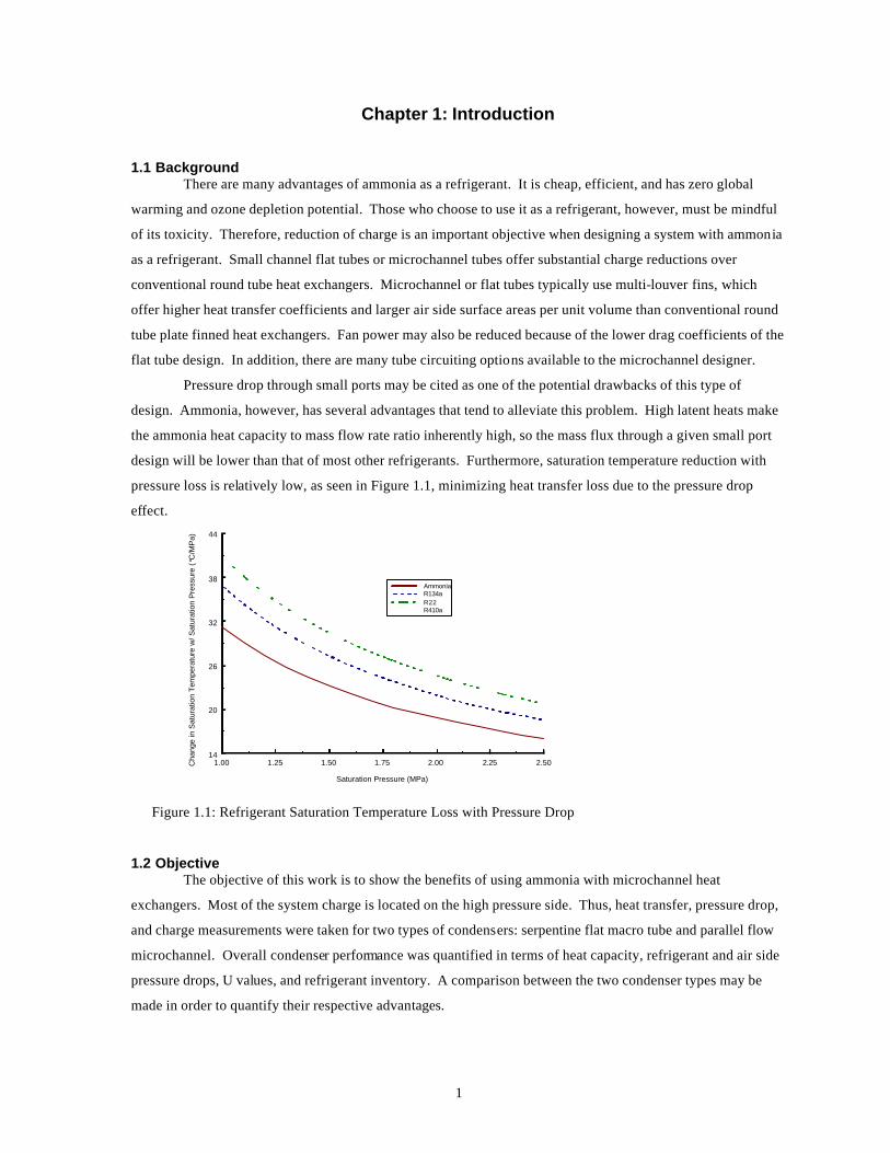
Pressure drop through small ports may be cited as one of the potential drawbacks of this type of
design. Ammonia, however, has several advantages that tend to alleviate this problem. High latent heats make
the ammonia heat capacity to mass flow rate ratio inherently high, so the mass flux through a given small port
design will be lower than that of most other refrigerants. Furthermore, saturation temperature reduction with
pressure loss is relatively low, as seen in Figure 1.1, minimizing heat transfer loss due to the pressure drop
effect.
1.00 1.25 1.50 1.75 2.00 2.25 2.50
Saturation Pressure (MPa)
14
20
26
32
38
44
Cha
nge
in S
atur
atio
n T
empe
ratu
re w
/ Sat
urat
ion
Pre
ssur
e (°
C/M
Pa)
AmmoniaR134aR22R410a
Figure 1.1: Refrigerant Saturation Temperature Loss with Pressure Drop
1.2 Objective The objective of this work is to show the benefits of using ammonia with microchannel heat
exchangers. Most of the system charge is located on the high pressure side. Thus, heat transfer, pressure drop,
and charge measurements were taken for two types of condensers: serpentine flat macro tube and parallel flow
microchannel. Overall condenser performance was quantified in terms of heat capacity, refrigerant and air side
pressure drops, U values, and refrigerant inventory. A comparison between the two condenser types may be
made in order to quantify their respective advantages.

2
Although most of the charge reduction potential is realized through the use of a microchannel
condenser, system charge was also measured to provide a baseline comparison to other ammonia chillers.
Charge per system capacity can be calculated and compared to other chillers to give an idea of how air cooled
commercial systems could benefit from microchannel technology.
There has been previous research on microchannel heat transfer and pressure drop characteristics.
Comparing ammonia microchannel heat transfer and pressure drop results to predictions from existing
correlations developed using other refrigerants and port diameters is necessary to verify design models. A finite
difference model was developed to predict heat transfer, pressure drop, and refrigerant inventory using available
correlations.
Since ammonia is a “new” fluid in microchannel heat exchangers, it is important to gain an
understanding of how it behaves within the exchanger tubes and headers. Understanding this behavior will
facilitate heat exchanger design and circuiting. Refrigerant header mal-distribution to parallel tubes reduces
exchanger capacity. Quantifying and understanding the effects of header mal-distribution could lead to better
circuiting designs; not just with ammonia, but with other fluids as well. Local air exit temperatures were taken
with a thermocouple grid. These temperatures give clues as to the two-dimensional distribution and properties
of ammonia within the condenser. An infrared camera measurement of tube surface temperatures was taken as
a secondary method to provide a more localized view of ammonia distribution. Furthermore, a single tube
condenser model was developed to verify the measurements and to help quantify the heat transfer losses from
header mal-distribution.
3
Chapter 2: Experimental Facility
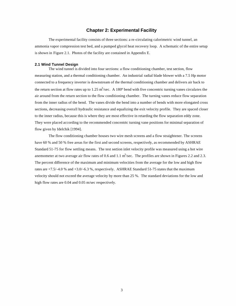
The experimental facility consists of three sections: a re-circulating calorimetric wind tunnel, an
ammonia vapor compression test bed, and a pumped glycol heat recovery loop. A schematic of the entire setup
is shown in Figure 2.1. Photos of the facility are contained in Appendix E.
2.1 Wind Tunnel Design The wind tunnel is divided into four sections: a flow conditioning chamber, test section, flow
measuring station, and a thermal conditioning chamber. An industrial radial blade blower with a 7.5 Hp motor
connected to a frequency inverter is downstream of the thermal conditioning chamber and delivers air back to
the return section at flow rates up to 1.25 m3/sec. A 180° bend with five concentric turning vanes circulates the
air around from the return section to the flow conditioning chamber. The turning vanes reduce flow separation
from the inner radius of the bend. The vanes divide the bend into a number of bends with more elongated cross
sections, decreasing overall hydraulic resistance and equalizing the exit velocity profile. They are spaced closer
to the inner radius, because this is where they are most effective in retarding the flow separation eddy zone.
They were placed according to the recommended concentric turning vane positions for minimal separation of
flow given by Idelchik [1994].
The flow conditioning chamber houses two wire mesh screens and a flow straightener. The screens
have 60 % and 50 % free areas for the first and second screens, respectively, as recommended by ASHRAE
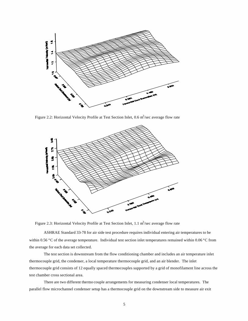
Standard 51-75 for flow settling means. The test section inlet velocity profile was measured using a hot wire
anemometer at two average air flow rates of 0.6 and 1.1 m3/sec. The profiles are shown in Figures 2.2 and 2.3.
The percent difference of the maximum and minimum velocities from the average for the low and high flow
rates are +7.5/-4.0 % and +3.0/-6.3 %, respectively. ASHRAE Standard 51-75 states that the maximum
velocity should not exceed the average velocity by more than 25 %. The standard deviations for the low and
high flow rates are 0.04 and 0.05 m/sec respectively.
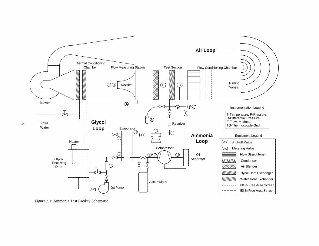
Figure 2.1: Ammonia Test Facility Schematic
4
T P T
T T
P
F
F
T
T
T D D
M
P T TG TG
Jet Pump
Accumulator
Compressor
Evaporator
Glycol Receiving
Drum
Heater
Receiver
Blower
Oil Separator
Test Section
Nozzles
Thermal Conditioning Chamber Flow Measuring Station Flow Conditioning Chamber
Turning Vanes
Instrumentation Legend
T-Temperature, P-Pressure, D-Differential Pressure, F-Flow, M-Mass, TG-Thermocouple Grid
Equipment Legend
Shut-off Valve
Metering Valve
Flow Straightener
Condenser
Glycol Heat Exchanger
Water Heat Exchanger
Air Blender
60 % Free Area Screen
50 % Free Area Sc reen
Air Loop
Ammonia Loop
Glycol Loop
Cold Water
5
Figure 2.2: Horizontal Velocity Profile at Test Section Inlet, 0.6 m3/sec average flow rate
Figure 2.3: Horizontal Velocity Profile at Test Section Inlet, 1.1 m3/sec average flow rate
ASHRAE Standard 33-78 for air side test procedure requires individual entering air temperatures to be
within 0.56 °C of the average temperature. Individual test section inlet temperatures remained within 0.06 °C from
the average for each data set collected.
The test section is downstream from the flow conditioning chamber and includes an air temperature inlet
thermocouple grid, the condenser, a local temperature thermocouple grid, and an air blender. The inlet
thermocouple grid consists of 12 equally spaced thermocouples supported by a grid of monofilament line across the
test chamber cross sectional area.
There are two different thermo couple arrangements for measuring condenser local temperatures. The
parallel flow microchannel condenser setup has a thermocouple grid on the downstream side to measure air exit
6
temperatures. This grid, also on monofilament line, has 30 thermocouples. There are 6 equally spaced columns of
thermocouples across the condenser face. There are 3 rows in the first pass, and 2 in the second. The microchannel
condenser has two passes with an unequal number of tubes per pass. So the thermocouple rows are equally spaced
within the area occupied for a given pass, but the row spacing for one pass is different from the other. Therefore,
each thermocouple represents the air exit temperature from a given area of the condenser that is approximately equal
to all the other grid areas. The serpentine macrochannel tube condenser has insulated surface thermocouples
attached to the tube bends instead of an air thermocouple grid to provide local temperature distribution.
An air blender mixes the stratified air exit temperature profile (caused by superheated and subcooled zones)
from the condenser before entering the flow measuring station. The entire test section is insulated with 1” thick
Celotex Tuff-R insulation above additional loose insulation.
The flow measuring station is a double nozzle array (0.1524 m (6”) and 0.127 m (5”) bore) with pressure
taps on the centerline of all four duct walls both upstream and downstream of the nozzles. Unobstructed flow
distances, clearances, nozzle geometry, and pressure tap locations all meet ASHRAE Standard 33-78 for air flow
and temperature measuring apparatus. Nozzle throat thermocouples measure test section air exit temperatures.
The thermal conditioning chamber consists of two heat exchangers that remove heat from the re-circulating
air flow. One transfers heat to the evaporator on the ammonia test bed via the glycol loop, and the other uses cold
city water to remove heat generated by compressor and blower work. Both tube side flow rates can be
independently controlled by metering valves to provide the required heat removal.
2.2 Ammonia Chiller Setup The ammonia test bed holds the compressor, evaporator, tubing, and related comp onents. Details of the
compressor and evaporator are listed in Appendix E. The compressor is a Bitzer W2TA two cylinder, open
reciprocating type with a direct drive coupling to a 7.5 Hp motor controlled by a frequency inverter. An AC&R
helical oil separator removes mineral oil, Clavus G68, from the superheated ammonia with a manufacturer’s stated
efficiency of 99 % and returns it to the compressor crankcase. The superheated line enters the wind tunnel test
section to the condenser inlet, and subcooled ammonia exits the condenser and wind tunnel.
Two shut-off valves near the inlet and outlet of the test chamber can be used to isolate the condenser from
the rest of the loop. Turning the valves simultaneously while the system is at steady state isolates the condenser
charge. The loop is immediately turned off, and ammonia is drained through a junction valve on the subcooled line
to an evacuated aluminum sampling cylinder in an ice bath. The sampling cylinder is connected to the junction
valve using a thermoplastic hose and quick connects fittings, which have double shut-off valves to ensure minimal
leakage.
At steady state, subcooled ammonia exits the condenser and enters an in-line, high pressure steel sight
glass. The sight glass not only provides a means to visually check if there is liquid ammonia flowing from the
condenser, but it also serves as a receiver. From the receiver flows single-phase liquid ammonia to a Micromotion
Elite CMF025 mass flow meter, which measures mass flow rate and density. The liquid ammonia then passes
through a needle metering valve that functions as an expansion valve to flash refrigerant to the evaporator. The
evaporator is an Alpha Laval NB26 Nickel brazed plate design with an internal volume of 984 cm3. The warm
7
glycol from the heat recovery loop evaporates ammonia. The ammonia flows downward as it travels through the
evaporator (despite the recommended up-flow configuration for maximum heat exchange) to ensure positive return
of the small quantities of oil back to the compressor. A suction line accumulator is used to prevent liquid slugging
of the compressor upon startup, since liquid ammonia tends to collect in the suction line after shutdown because of
the down-flow configuration and the absence of a solenoid valve in the liquid line. Two shut-off valves can easily
isolate the accumulator from the rest of the ammonia loop.
An absolute pressure transducer at the inlet to the condenser provides inlet refrigerant pressure. A
differential pressure transducer across the condenser gives ammonia pressure drop. Immersion thermocouples are
located at the inlet and outlet of the condenser. These pressure and temperature measurements are used to calculate
refrigerant side heat transfer. Other pressure transducers and immersion thermocouples around the ammonia loop
provide measurements necessary for system control.
2.3 Glycol Heat Recovery Loop The glycol circulates in a loop between a heat exchanger in the wind tunnel thermal conditioning chamber
and the evaporator on the chiller test bed. Warm glycol heats the ammonia at the evaporator and then cools the wind
tunnel air. An immersion heater provides additional heat to the glycol within a receiving drum at the outlet of the
wind tunnel heat exchanger for easy control when needed. A jet pump circulates the glycol at mass flow rates that
are controlled with a metering valve.
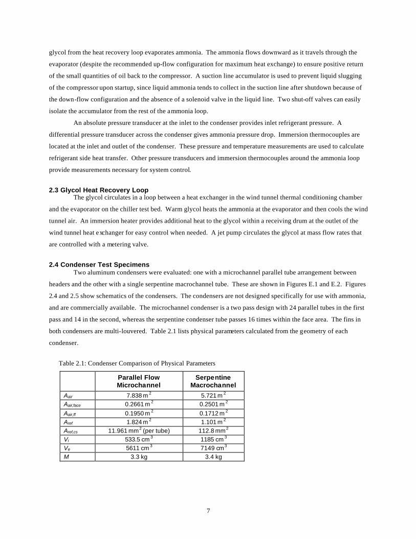
2.4 Condenser Test Specimens Two aluminum condensers were evaluated: one with a microchannel parallel tube arrangement between
headers and the other with a single serpentine macrochannel tube. These are shown in Figures E.1 and E.2. Figures
2.4 and 2.5 show schematics of the condensers. The condensers are not designed specifically for use with ammonia,
and are commercially available. The microchannel condenser is a two pass design with 24 parallel tubes in the first
pass and 14 in the second, whereas the serpentine condenser tube passes 16 times within the face area. The fins in
both condensers are multi-louvered. Table 2.1 lists physical parameters calculated from the geometry of each
condenser.
Table 2.1: Condenser Comparison of Physical Parameters
Parallel Flow Microchannel
Serpentine Macrochannel
Aair 7.838 m 2 5.721 m 2 Aair,face 0.2661 m 2 0.2501 m 2 Aair,ff 0.1950 m 2 0.1712 m 2 Aref 1.824 m 2 1.101 m 2 Aref,cs 11.961 mm2 (per tube) 112.8 mm2 Vi 533.5 cm 3 1185 cm 3 Ve 5611 cm 3 7149 cm3 M 3.3 kg 3.4 kg
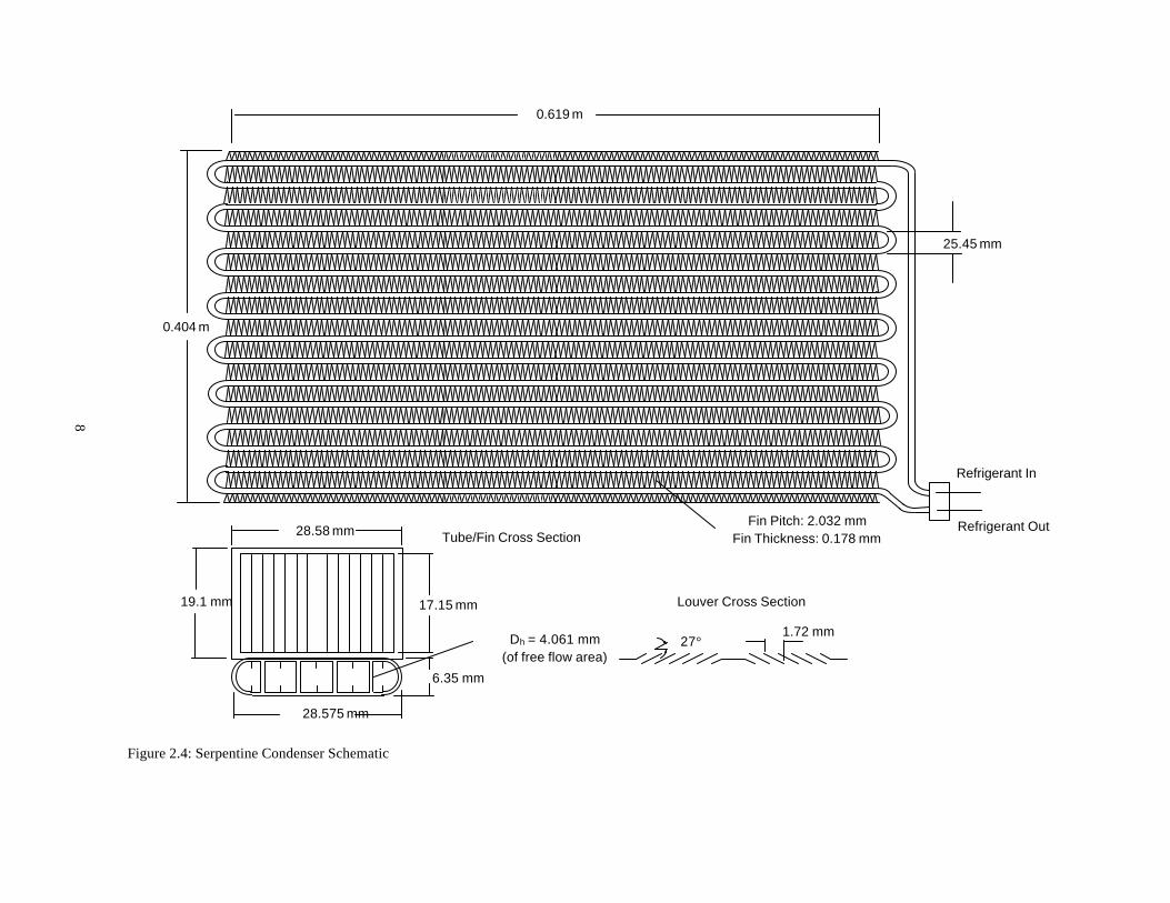
Figure 2.4: Serpentine Condenser Schematic
8
0.404 m
0.619 m
25.45 mm
Refrigerant In
Refrigerant Out
Dh = 4.061 mm (of free flow area)
Tube/Fin Cross Section
19.1 mm
28.58 mm
17.15 mm
6.35 mm
28.575 mm
27° 1.72 mm
Louver Cross Section
Fin Pitch: 2.032 mm Fin Thickness: 0.178 mm
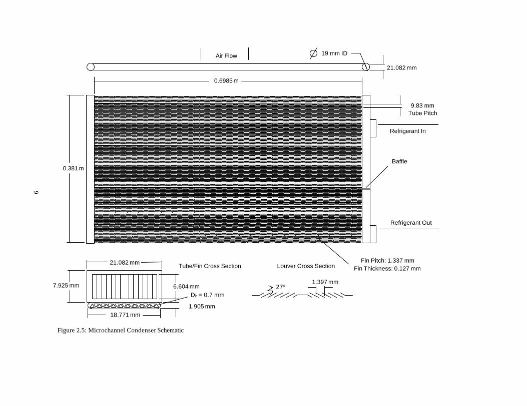
Figure 2.5: Microchannel Condenser Schematic
9
21.082 mm
19 mm ID
0.6985 m
0.381 m
9.83 mm Tube Pitch
Refrigerant In
Refrigerant Out
Baffle
Air Flow
Dh = 0.7 mm
Tube/Fin Cross Section
7.925 mm
21.082 mm
6.604 mm
1.905 mm 18.771 mm
27° 1.397 mm
Louver Cross Section Fin Pitch: 1.337 mm
Fin Thickness: 0.127 mm
10
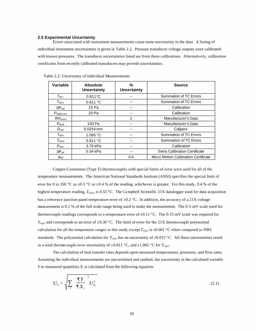
2.5 Experimental Uncertainty Errors associated with instrument measurements cause some uncertainty in the data. A listing of
individual instrument uncertainties is given in Table 2.2. Pressure transducer voltage outputs were calibrated
with known pressures. The transducer uncertainties listed are from these calibrations. Alternatively, calibration
certificates from recently calibrated transducers may provide uncertainties.
Table 2.2: Uncertainty of Individual Measurements
Variable Absolute Uncertainty
% Uncertainty
Source
Tair,i 0.811°C -- Summation of TC Errors Tair,o 0.811 °C -- Summation of TC Errors
∆Pnoz 15 Pa -- Calibration Pstatic,noz 20 Pa -- Calibration RHroom 2 Manufacturer’s Data Pamb 100 Pa -- Manufacturer’s Data Dnoz 0.0254 mm -- Calipers Tref,i 1.065 °C -- Summation of TC Errors Tref,o 0.811 °C -- Summation of TC Errors Pref,i 3.79 kPa -- Calibration ∆Pref 0.34 kPa -- Setra Calibration Certificate wref 0.4 Micro Motion Calibration Certificate
Copper-Constantan (Type T) thermocouples with special limits of error were used for all of the
temperature measurements. The American National Standards Institute (ANSI) specifies the special limit of
error for 0 to 350 °C as ±0.5 °C or ±0.4 % of the reading, whichever is greater. For this study, 0.4 % of the
highest temperature reading, Tref,i, is 0.55 °C. The Ca mpbell Scientific 21X datalogger used for data acquisition
has a reference junction panel temperature error of ±0.2 °C. In addition, the accuracy of a 21X voltage
measurement is 0.1 % of the full scale range being used to make the measurement. The 0-5 mV scale used for
thermocouple readings corresponds to a temperature error of ±0.11 °C. The 0-15 mV scale was required for
Tref,i and corresponds to an error of ±0.30 °C. The limit of error for the 21X thermocouple polynomial
calculation for all the temperature ranges in this study except Tref,i is ±0.001 °C when compared to NBS
standards. The polynomial calculation for Tref,i has an uncertainty of ±0.015 °C. All these uncertainties result
in a total thermocouple error uncertainty of ±0.811 °C, and ±1.065 °C for Tref,i.
The calculation of heat transfer rates depends upon measured temperatures, pressures, and flow rates.
Assuming the individual measurements are uncorrelated and random, the uncertainty in the calculated variable
Y to measured quantities Xi is calculated from the following equation.
UYX
UYi
Xi
i=
∑ ∂
∂
2
2 (2.1)
11
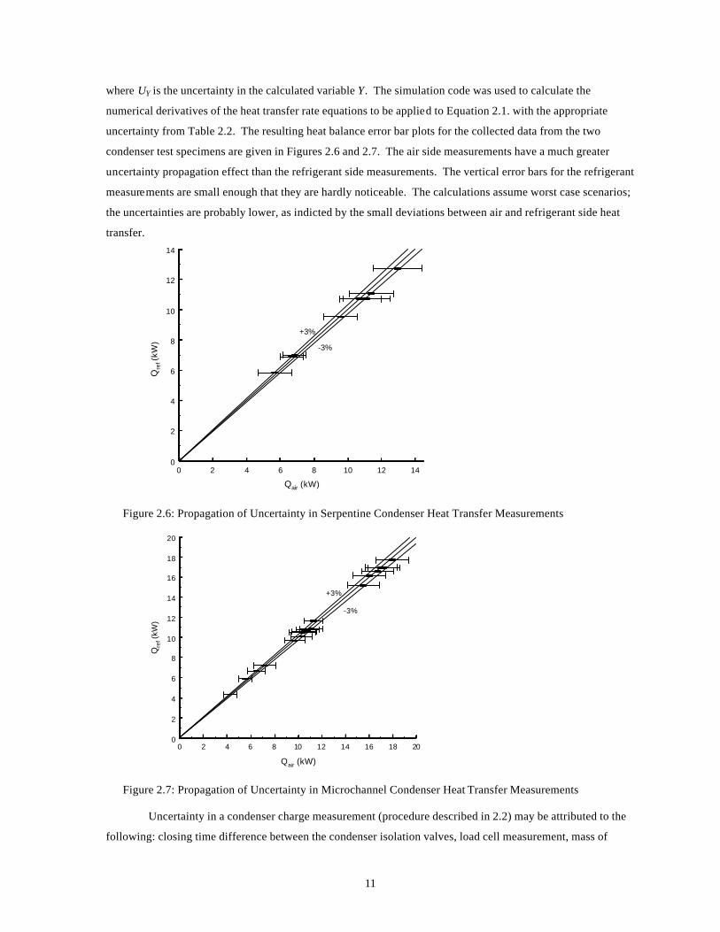
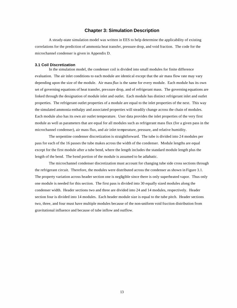
where UY is the uncertainty in the calculated variable Y. The simulation code was used to calculate the
numerical derivatives of the heat transfer rate equations to be applied to Equation 2.1. with the appropriate
uncertainty from Table 2.2. The resulting heat balance error bar plots for the collected data from the two
condenser test specimens are given in Figures 2.6 and 2.7. The air side measurements have a much greater
uncertainty propagation effect than the refrigerant side measurements. The vertical error bars for the refrigerant
measurements are small enough that they are hardly noticeable. The calculations assume worst case scenarios;
the uncertainties are probably lower, as indicted by the small deviations between air and refrigerant side heat
transfer.
0 2 4 6 8 10 12 14
Qair (kW)
0
2
4
6
8
10
12
14
Qre
f (kW
)
+3%
-3%
Figure 2.6: Propagation of Uncertainty in Serpentine Condenser Heat Transfer Measurements
0 2 4 6 8 10 12 14 16 18 20
Qair (kW)
0
2
4
6
8
10
12
14
16
18
20
Qre
f (kW
)
+3%
-3%
Figure 2.7: Propagation of Uncertainty in Microchannel Condenser Heat Transfer Measurements
Uncertainty in a condenser charge measurement (procedure described in 2.2) may be attributed to the
following: closing time difference between the condenser isolation valves, load cell measurement, mass of

12
vapor remaining in the condenser after draining the bulk charge, and the mass of refrigerant between the
condenser and the isolation valves during steady state. The experimental condenser charge is the change in
mass of the sampling cylinder and connection hose plus the mass of the vapor left after draining (calculated
from the internal volume and pressure and temperature measurements after draining) minus the mass of the
ammonia in the space between the condenser and the isolation valves (calculated from internal volume and
pressure and temperature measurements before condenser isolation). The closing time difference uncertainty
may be estimated from the product wref⋅(0.25 sec), where 0.25 sec is the estimated largest time difference
between closing times for each shut-off valve and wref is the refrigerant mass flow rate. The load cell used for
mass measurements has an uncertainty of ±0.1 g. The closing time difference uncertainty is added to the scale
uncertainty. The internal volumes of the condenser and of the dead space were each given a conservative
estimate of ±5 % uncertainty. Temperatures and pressures used in the charge calculation were given the
appropriate uncertainties from Table 2.2. Equation 2.1 applied to the charge calculation gives uncertainties of
±1.4 to 2.8 g and ±2.1 to 3.3 g for the serpentine and microchannel condensers, respectively. The mass flow
rates are higher for the microchannel condenser, thus its uncertainties are greater due to the propagation of valve
closing time difference error, the largest contributor to charge uncertainty.
13
Chapter 3: Simulation Description
A steady-state simulation model was written in EES to help determine the applicability of existing
correlations for the prediction of ammonia heat transfer, pressure drop, and void fraction. The code for the
microchannel condenser is given in Appendix D.
3.1 Coil Discretization In the simulation model, the condenser coil is divided into small modules for finite difference
evaluation. The air inlet conditions to each module are identical except that the air mass flow rate may vary
depending upon the size of the module. Air mass flux is the same for every module. Each module has its own
set of governing equations of heat transfer, pressure drop, and of refrigerant mass. The governing equations are
linked through the designation of module inlet and outlet. Each module has distinct refrigerant inlet and outlet
properties. The refrigerant outlet properties of a module are equal to the inlet properties of the next. This way
the simulated ammonia enthalpy and associated properties will steadily change across the chain of modules.
Each module also has its own air outlet temperature. User data provides the inlet properties of the very first
module as well as parameters that are equal for all modules such as refrigerant mass flux (for a given pass in the
microchannel condenser), air mass flux, and air inlet temperature, pressure, and relative humidity.
The serpentine condenser discretization is straightforward. The tube is divided into 24 modules per
pass for each of the 16 passes the tube makes across the width of the condenser. Module lengths are equal
except for the first module after a tube bend, where the length includes the standard module length plus the
length of the bend. The bend portion of the module is assumed to be adiabatic.
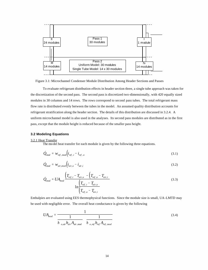
The microchannel condenser discretization must account for changing tube side cross sections through
the refrigerant circuit. Therefore, the modules were distributed across the condenser as shown in Figure 3.1.
The property variation across header section one is negligible since there is only superheated vapor. Thus only
one module is needed for this section. The first pass is divided into 30 equally sized modules along the
condenser width. Header sections two and three are divided into 24 and 14 modules, respectively. Header
section four is divided into 14 modules. Each header module size is equal to the tube pitch. Header sections
two, three, and four must have multiple modules because of the non-uniform void fraction distribution from
gravitational influence and because of tube inflow and outflow.
14
Figure 3.1: Microchannel Condenser Module Distribution Among Header Sections and Passes
To evaluate refrigerant distribution effects in header section three, a single tube approach was taken for
the discretization of the second pass. The second pass is discretized two-dimensionally, with 420 equally sized
modules in 30 columns and 14 rows. The rows correspond to second pass tubes. The total refrigerant mass
flow rate is distributed evenly between the tubes in the model. An assumed quality distribution accounts for
refrigerant stratification along the header section. The details of this distribution are discussed in 3.2.4. A
uniform microchannel model is also used in the analyses. Its second pass modules are distributed as in the first
pass, except that the module height is reduced because of the smaller pass height.
3.2 Modeling Equations
3.2.1 Heat Transfer The mo del heat transfer for each module is given by the following three equations.
( )&, , ,Q w i imod ref mod ref i ref o= − (3.1)
( )&, , ,Q w i imod air mod air o air i= − (3.2)
( ) ( )( )( )
&
ln
, , , ,
, ,
, ,
Q UAT T T T
T T
T T
mod modref i air o ref o air i
ref i air o
ref o air i
=− − −
−
−
(3.3)
Enthalpies are evaluated using EES thermophysical functions. Since the module size is small, UA-LMTD may
be used with negligible error. The overall heat conductance is given by the following
UA
h A h A
mod
o air air air mod o ref ref ref mod
=+
11 1
η η, , , ,
(3.4)
Pass 1 30 modules
Pass 2 Uniform Model: 30 modules
Single Tube Model: 14 x 30 modules
II 24 modules
III 14 modules
I 1 module
IV 14 modules
15
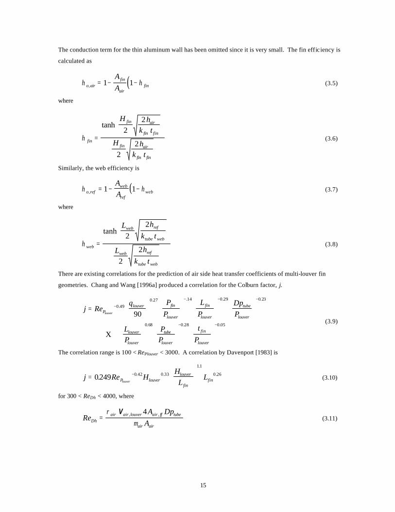
The conduction term for the thin aluminum wall has been omitted since it is very small. The fin efficiency is
calculated as
( )η ηo airfin
airfin
AA, = − −1 1 (3.5)
where
η fin
fin air
fin fin
fin air
fin fin
H hk t
H hk t
=
tanh
22
22
(3.6)
Similarly, the web efficiency is
( )η ηo refweb
refweb
AA, = − −1 1 (3.7)
where
η web
web ref
tube web
web ref
tube web
L hk t
L hk t
=
tanh
22
22
(3.8)
There are existing correlations for the prediction of air side heat transfer coefficients of multi-louver fin
geometries. Chang and Wang [1996a] produced a correlation for the Colburn factor, j.
j ReP
PL
PDpP
LP
PP
tP
Plouver fin
louver
fin
louver
tube
louver
louver
louver
tube
louver
fin
louver
louver=
−
− − −
− −
0 490 27 14 0 29 0 23
0 68 0 28 0 05
90.
. . . .
. . .
X
θ
(3.9)
The correlation range is 100 < RePlouver < 3000. A correlation by Davenport [1983] is
j Re HHL
LP louverlouver
finfinlouver
=
−0249 0 42 0 33
1 1
0 26. . .
.
. (3.10)
for 300 < ReDh < 4000, where
ReA Dp
ADhair air louver air ff tube
air air
=ρ
µ V , ,4
(3.11)
16
and Lfin and Hlouver are in mm. Achaichia and Cowell [1988] produced a correlation for the Stanton number, St.
StRe
PP
RePP
PP
P
fin
louverlouver
louver
Ptube
louver
fin
louver
louver
louver
=
− − +
−
−
1554
0936243
176 0995
0 59
0 09
.
. . .
X .
.
θ
θ (3.12)
This correlation was developed for plate and tube louver fin geometries for RePlouver > 75.
The correlations used to predict air side heat transfer for this study were derived from experimental
data on the tested condensers. Several calculation techniques were explored. They are explained in 4.1.2. The
equation used to predict microchannel condenser air side heat transfer coefficients is
h Re Re
Re Re
air P P
P P
louver louver
louver louver
= − + −
+ −− −
9364 1848 0005522
8 25 10 4 773 10
2
6 3 9 4
. . .
. x . x (3.13)
where hair is in W/m2-°C. The equation does not include geometrical parameters since it is for a single
condenser only. The equation for the serpentine condenser is
h Re Re
Re Reair P P
P P
louver louver
louver louver
= − + −
+ −− −
127 7 1598 0 004154
504 10 2 206 10
2
6 3 9 4
. . .
. x . x (3.14)
The calculation of the refrigerant side heat transfer coefficient is dependent upon the refrigerant phase.
In the single-phase regions of the condenser, the Gnielinski [1976] correlation is used. The Gnielinski
correlation is given by
( )
( )Nu
fRe Pr
fPr
DL
PrPr
F
F tube w
=−
+ −+
2
1000
1 12 72
11
23
23 0 11
.
.
(3.15)
where
f ReF = −007911
4. (3.16)
This is generally considered the most accurate available correlation for 2300 < Re < 10000. The correlation
accuracy improves when Re > 10000.
Several two-phase refrigerant heat transfer coefficient correlations were explored. Dobson [1998]
gives two correlations for two different flow regimes. These were developed using inner tube diameters of 3.14
mm and 7.04 mm with the following refrigerants: R-12, R-22, R-134a, and near-azeotropic blends of R-32/R-
125 in 50/50 and 60/40 percent combinations. The mass flux ranges are 75-800 kg/m2-sec for the 3.14 mm tube
and 25-800 kg/m2-sec for the 7.04 mm tube.
Dobson’s correlations reflect the modes of heat transfer. In the gravity dominated flow regime,
laminar film condensation in the upper part of the tube is the primary heat transfer mode, whereas in shear
17
dominated flows, forced convective condensation is the primary mode. Dobson’s wavy correlation separates
the heat transfer by film condensation in the upper part of the tube from the forced convective heat transfer in
the bottom. This correlation is
( )Nu
ReX
Ga PrJa
Nuvo
tt
l
lforced=
+
+
−0231 111
2 10 12
0 58
0 25.
.arccos.
.
.α
π (3.17)
where
ReGD
vov
=µ
(3.18)
Xx
xttv
l
l
v
=−
1 0 875 0 5 0 125. . .ρρ
µµ
(3.19)
( )Ga gD
l l vl
= −ρ ρ ρµ
3
2 (3.20)
Prckll p l
l
=µ ,
(3.21)
( )Ja
c T Til
p l sat w
lv
=−,
(3.22)
and
( )Nu Re Pr Xforced l l l tt= 0 0195 0 8 0 4. . . φ (3.23)
where
( )φl tttt
cXc
X= +1376 1
2. (3.24)
and
( )Re
GD xl
l
=−1
µ (3.25)
The values of c1 and c2 depend on the liquid Froude number, Frl.
FrG
gDll
=2
2ρ (3.26)
For 0 < Frl ≤ 0.7,
c Fr Frl l124172 548 1564= + −. . . (3.27a)
c Frl2 1773 0169= −. . (3.27b)
18
For Frl > 0.7,
c1 7 242= . (3.28a)
c2 1655= . (3.28b)
For annular flow Dobson gives the following correlation for Nusslet number.
Nu Re PrXl l
tt
= +
0023 1
2 220 8 0 40 89.
.. .. (3.29)
Dobson recommends using Equation 3.29 when Gref ≥ 500 kg/m2-sec. When Gref < 500 kg/m2-sec, Equation
3.17 should be used if Frso < 20, and Equation 3.29 should be used if Frso > 20. Frso is Soliman’s [1982]
modified Froude number.
Fr ReX
X Gaso ltt
tt
=+
0 025
1 109 11 590 039 1 5
0 5...
. .
. (3.30a)
for Rel ≤ 1250, and
Fr ReX
X Gaso ltt
tt
=+
126
1 109 11 040 039 1 5
0 5...
. .
. (3.30b)
for Rel >1250. Rel is the superficial liquid Reynolds number.
( )Re
GD xl
l
=−1
µ (3.31)
Shah [1978] developed a film condensation correlation from a wide variety of experimental data. The fluids
included in the study were water, R-11, R-12, R-22, R-113, methanol, ethanol, benzene, toluene, and
trichloroethylene condensing in pipes with internal diameters ranging from 7 to 40 mm. The mass flux range
covered is 11-211 kg/m2-sec. It is given by
( ) ( )Nu Re Pr x
x x
PP
lo l
crit
= − +−
0023 138 10 8 0 4 0 8
0 76 0 04
0 38... . .
. .
. (3.32)
where
ReGD
lol
=µ
(3.33)
3.2.2 Pressure Drop Air side pressure drop is used to evaluate condenser performance. Several existing correlations for
pressure drop across multi-louver fins and flat tubes were used and compared with experimental data from the
microchannel and serpentine condensers. The correlations give Fanning friction factor as a function of
19
Reynolds number and condenser geometry. For each correlation, the pressure drop is calculated from the
friction factor by
∆P Kairair i air o
air louver cair i
air o
=+
+ − + −
ρ ρσ
ρρ
, ,,
,
,21 2 12 2V
( )++
− − −
fA
AKF
air
air ff
air i
air i air oe
air i
air o,
,
, ,
,
,
21 2
ρρ ρ
σρρ
(3.34)
Kc and Ke are the contraction and expansion loss coefficients, respectively. They are evaluated using a curve fit
to the data presented in Kays and London [1998] for a multiple square tube heat exchanger core. The following
equations are curve fits for Re = ∞, as recommended for surfaces with frequent fin interruptions. σ is the ratio
of free flow area to face area (or frontal area).
Kc = + −0 3995 0 03674 0 43561 2. . .σ σ (3.35)
Ke = − +0 99333 194515 095455 2. . .σ σ (3.36)
Chang and Wang’s [1996b] correlation developed for multi-louvered fins with corrugated channels is
f ReA
A
A
AF Pair
air tube
air louver
airlouver
=
−0862 0 488
0 706 1 04
. .
,
.
,.
(3.37)
for 100 < RePlouver < 1000. Davenport’s [1983] correlation developed for the same flow arrangement is
f ReHP
LH
HF Plouver
louver
louver
finfinlouver
=
−
−
0 494 0 39
0 33 1 1
0 46. .
. .
. (3.38)
for 1000 < ReDh < 4000. All dimensional variables are in mm. Achaichia’s [1988] correlation was developed
for plate and tube louver fin geometry and is given by
f f P P P LF o fin louver tube louver= −0895 1 07 0 22 0 25 0 26 0 33. . . . . . (3.39)
where
( )f Reo PRe
louver
Plouver= −596 0 318 2 25. log( ) . (3.40)
for 150 < ReDh < 3000. Again, all dimensional variables are in mm. The microchannel condenser air pressure
drop data in this study yields the following curve fit equation.
∆P Re Re Reair P P Plouver louver louver= − − + +− −303 009095 2 479 10 8 716 104 2 9 3. . . x . x (3.41)
where ∆Pair is in Pa. The serpentine condenser data gives
∆P Re Re Reair P P Plouver louver louver= − + − +− −17 09 01355 6 711 10 1529 105 2 7 3. . . x . x (3.42)
20
On the refrigerant side, the general form of the pressure drop relation used for the single-phase regions
is
− =dPdz
fG vDF
2 2
(3.43)
Churchill’s [1977] friction factor was used in the model. It is an explicit representation for turbulent friction
factor in both laminar and turbulent regions with smooth or rough pipes.
( )f
fRe A Bc
F= =
+
+
28 112
32
112
(3.44)
where
A
Re D
=
+
2 4571
7027
0 9
16
. ln.
. ε (3.45)
and
BRe
=
37 530 16, (3.46)
For the two-phase region, de Souza’s [1995] correlation was used. This correlation was developed
using tube diameters ranging from 7.75 mm to 10.92 mm with R-134a, R-12, R-22, MP-39, and R-32/125. The
testing covers the entire quality range with mass fluxes from 50 to 600 kg/m2-sec. The overall pressure drop
from friction across a quality range is
∆ ∆∆
P Px
dxf lo lo= ∫1 2φ (3.47)
where ∆Plo is the frictional pressure drop of the total mixture flowing as a liquid, given by
∆Pf G L
Dlolo
l
=2 2
ρ (3.48)
where flo is the liquid Fanning friction coefficient. flo is given from the Haaland correlation, [White, 1986].
f
Re D
lo
lo
=
+
1
12 9669
37
1 11 2
. log.
.
.ε (3.49)
where Relo is calculated from Equation 3.33. φ 2lo is the two-phase multiplier, which de Souza gives as
( ) ( )φ lo ttx X2 2 1 75 0 41261 1 1 0 9524= + − +Γ Γ. .. (3.50)
where Xtt is the Lockhart-Martinelli parameter defined in Equation 3.19, and Γ is
21
Γ =
ρ
ρµµ
l
v
v
l
0 5 0 125. .
(3.51)
If the quality does not vary (the two-phase flow is adiabatic), then the two-phase multiplier does not have to be
averaged, and ∆Pf is calculated from the product of the two-phase multiplier and ∆Plo.
Condensation gives a pressure increase to the mixture due to deceleration. This deceleration term is
given by
( )( )
( )( )∆P G
x x x xdec
o
v o
o
l o
i
v i
i
l i
= − +−
−
− +
−
−
22
22
21
1
1
1ρ α ρ α ρ α ρ α (3.52)
where α is the void fraction. de Souza recommends the Zivi void fraction correlation, which is given along
with other correlations in 3.2.3. The total two-phase pressure drop is then
∆ ∆ ∆P P Ptot f dec= − (3.53)
3.2.3 Refrigerant Inventory The mass of a module in the model is calculated by
( )( )m A Lmod ref cs mod v l= + −, ρ α ρ α1 (3.54)
where Lmod is the length of the module, Aref,cs the tube side cross sectional area, and α the void fraction. α is
equal to one for single-phase vapor and zero for single-phase liquid.
Several void fraction correlations were used and compared in the model to predict two-phase charge.
Zivi’s [1964] correlation was developed from a minimization of entropy argument and is given by
αρρ
=
+−
1
11
23
xx
v
l
(3.55)
Butterworth [1949] proposed a correlation similar to Zivi’s with an Xtt type dependence.
αρρ
µ
µ
=
+−
1
1 0 281 0 64 0 36 0 07
.. . .
xx
v
l
l
v
(3.56)
Newell’s [1999] correlation combines the effects of the Lockhart-Martinelli parameter, Xtt, with a Froude rate,
Ft. Ft is related to the ratio of the vapor flow’s power to the power required to move liquid from the bottom to
the top of a tube. The correlation is given by
α = + +
−
11 0 321
FtX tt
.
(3.57)
where Xtt is from Equation 3.19 and Ft is
22
( )FtG xx gDv
=−
2 3
21 ρ (3.58)
3.2.4 Header Modeling The header sections are assumed to be adiabatic in the model. Pressure drop effects from sudden
changes in area and from tube inflow and outflow in the headers are modeled using empirical relations
developed by Idelchik [1994], which are given in the code in Appendix D. Refrigerant inventory in the headers
was also accounted for in the model. In header section one, the refrigerant properties are uniform and known
from experimental data, so the charge can be determined with little difficulty. In header sections two, three, and
four, however, the refrigerant is in the two-phase form. Therefore, a scheme for calculating void fraction must
be used.
Zietlow’s [1995] visual experiments for microchannel tube outflow into a header show the flow to be
mostly dispersed liquid with a thin film on the wall. Also, the trajectories of the liquid exiting the tubes in these
experiments indicates that gravity is a significant force on the liquid. Zietlow developed a method to predict
void fraction in the outlet header based upon fundamental equations of motion and from conservation of
momentum. This method was used in header sections two and four of the model. There are several
assumptions in Zietlow’s method, including equivalent mass flow rates in all the condenser tubes and negligible
interfacial shear forces.
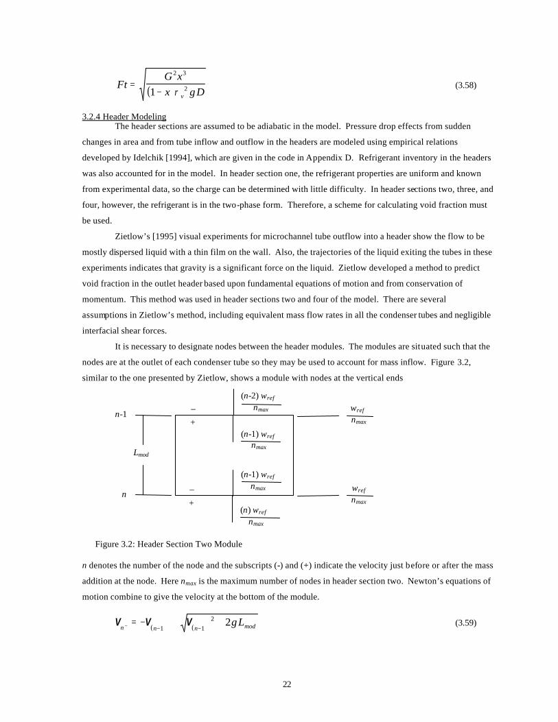
It is necessary to designate nodes between the header modules. The modules are situated such that the
nodes are at the outlet of each condenser tube so they may be used to account for mass inflow. Figure 3.2,
similar to the one presented by Zietlow, shows a module with nodes at the vertical ends
Figure 3.2: Header Section Two Module
n denotes the number of the node and the subscripts (-) and (+) indicate the velocity just before or after the mass
addition at the node. Here nmax is the maximum number of nodes in header section two. Newton’s equations of
motion combine to give the velocity at the bottom of the module.
( ) ( )V V Vn n n modgL− + += − + +
− −1 12 2 (3.59)
Lmod
n-1
n
(n-2) wref
(n-1) wref
–
+
(n-1) wref
(n) wref
nmax
nmax
nmax
nmax
–
+
wref nmax
nmax wref
23
Thus, at the bottom of the module of the top tube in header section two (before the next node), the velocity of
the liquid is (2gLmod)½. The conservation of momentum at a node gives
( )V
Vn
nn
n+
−
=− 1
(3.60)
From the continuity equation the cross sectional area of the liquid is given by
( ) ( )
( )( )Ax n w
ncs l
ref
max l n n
, =− −
+− +−
2 1 1
1ρ V V
(3.61)
and the void fraction is then determined by
α = −1AA
cs l
cs
, (3.62)
Header section three conditions are very similar to those in the inlet header of the microchannel
condenser in Zietlow’s work. Both have a header tube delivering two-phase refrigerant to horizontal
microchannel tubes. The inlet to Zietlow’s condenser is a vertical pipe at the top of the header. Header section
three is also fed vertically. Therefore, header section three void fractions were modeled after Zietlow’s inlet
header method.
Void fraction can be defined in terms of a slip ratio, S, by
αρρ
=+
−
1
11 x
xSn
n
v
l
(3.63)
Hughmark [1962] defined a variable KH as the inverse slip ratio.
KSH =1
(3.64)
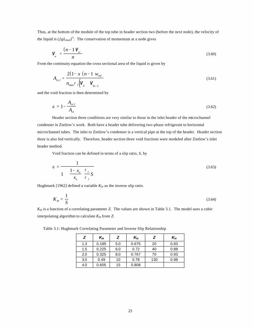
KH is a function of a correlating parameter Z. The values are shown in Table 3.1. The model uses a cubic
interpolating algorithm to calculate KH from Z.
Table 3.1: Hughmark Correlating Parameter and Inverse Slip Relationship
Z KH Z KH Z KH
1.3 0.185 5.0 0.675 20 0.83 1.5 0.225 6.0 0.72 40 0.88 2.0 0.325 8.0 0.767 70 0.93 3.0 0.49 10 0.78 130 0.98 4.0 0.605 15 0.808
24
Z is given by
( )Z
Re Frp p
=−
1 2
11
4β (3.65)
where
( )ReG Dn
l v l
=+ −µ α µ µ
(3.66)
Gw
nn
An
refmax
cs
=−
−
1
1
(3.67)
FrgD
G xn n
v
=
12
β ρ (3.68)
and
βρρ
=+
−
1
11 x
xn
n
v
l
(3.69)
p1 and p2 are 0.167 and 0.125, respectively, as defined by Hughmark. Zietlow, however, has optimized these
parameters for the prediction of refrigerant inventory in the inlet header of his microchannel condenser. The
parameters p1 and p2 for this scenario are 0.136 and 0.724, respectively. Gn is derived from the conservation of
momentum at each node. Again, mass flow rate is distributed evenly among the second pass tubes. α can be
approximated from any of the correlations in 3.2.3 so that the calculation becomes explicit. Here nmax is the
maximum number of nodes in header section three. xn is given an arbitrary distribution. A lthough not based
solely upon experimental data, educated assumptions can be made to give an appropriate distribution.
Zietlow’s flow visualization experiments indicate dispersed liquid flow at the top of the header with a
transition to dispersed bubble flow at the lower-middle region of the header. Gravity separates the liquid from
the flow as the inertial forces abate farther down the header. Thus the quality profile should start at zero at the
bottom of the header. A simple distribution function that starts at zero quality and continues to the maximum
quality xmax along the total length of the header Lheader3 is given by the following first order equation.
x y xy
Lmaxheader
a
( ) =
3
(3.70)
where y is the distance from the bottom of the header and a is the exponent giving the profile its particular
shape.
Zietlow also observed that as inlet quality increased, the dispersed liquid region occupied more of the
header than the dispersed bubble flow region. So as header inlet quality increases, the average quality of the
25
distribution in the header increases. Because no other data is available, the distribution of quality in the model
assumes an average profile quality equal to the header section three inlet quality. So the average of Equation
3.70 along the length of the header must equal the header section three inlet quality xi.
xL
xy
Ldyi
header3max
header3
aLheader3
=
∫
10
(3.71)
This yields
axxmax
i= − 1 (3.72)
The profile is given in terms of node numbers by
x xn n
nn maxmax
max
xxmax
i
=−
−
1
(3.73)
The appropriate value for xmax is discussed in 4.3.3.
26
Chapter 4: Results & Discussion
Overall heat transfer performance, pressure drop, and charge measurements were taken for each
condenser. A listing of all the serpentine and microchannel condenser data is given in Table A.1 and Table A.2
in Appendix A.
Overall condenser heat transfer performance is quantified in terms of U values for different air flow
rates. Total heat transfer is compared to model predictions. Air side local heat transfer coefficients were
determined using several techniques and are compared to existing correlations. Experimentally obtained air and
refrigerant side pressure drop results are compared to existing correlation predictions. Refrigerant inventory
measurements are compared to model results using different void fraction model predictions. Local
temperature distribution data were also collected by several means, are compared, and used to quantify the
effects of mal-distribution of refrigerant in the microchannel condenser headers.
4.1 Serpentine Condenser
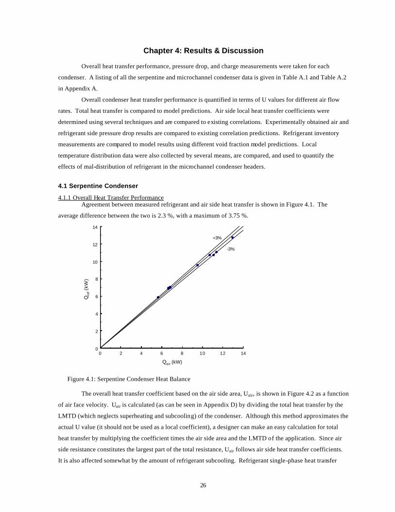
4.1.1 Overall Heat Transfer Performance Agreement between measured refrigerant and air side heat transfer is shown in Figure 4.1. The
average difference between the two is 2.3 %, with a maximum of 3.75 %.
0 2 4 6 8 10 12 14
Qair (kW)
0
2
4
6
8
10
12
14
Qre
f (kW
)
+3%
-3%
Figure 4.1: Serpentine Condenser Heat Balance
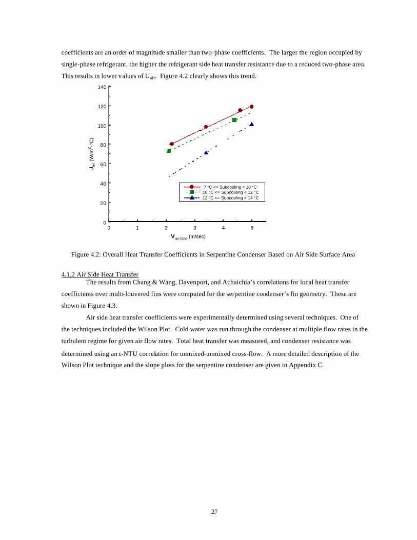
The overall heat transfer coefficient based on the air side area, Uair, is shown in Figure 4.2 as a function
of air face velocity. Uair is calculated (as can be seen in Appendix D) by dividing the total heat transfer by the
LMTD (which neglects superheating and subcooling) of the condenser. Although this method approximates the
actual U value (it should not be used as a local coefficient), a designer can make an easy calculation for total
heat transfer by multiplying the coefficient times the air side area and the LMTD of the application. Since air
side resistance constitutes the largest part of the total resistance, Uair follows air side heat transfer coefficients.
It is also affected somewhat by the amount of refrigerant subcooling. Refrigerant single-phase heat transfer
27
coefficients are an order of magnitude smaller than two-phase coefficients. The larger the region occupied by
single-phase refrigerant, the higher the refrigerant side heat transfer resistance due to a reduced two-phase area.
This results in lower values of Uair. Figure 4.2 clearly shows this trend.
0 1 2 3 4 5
Vair,face (m/sec)
0
20
40
60
80
100
120
140U
air (
W/m
2 -°C
)
7 °C <= Subcooling < 10 °C10 °C <= Subcooling < 12 °C12 °C <= Subcooling < 14 °C
Figure 4.2: Overall Heat Transfer Coefficients in Serpentine Condenser Based on Air Side Surface Area
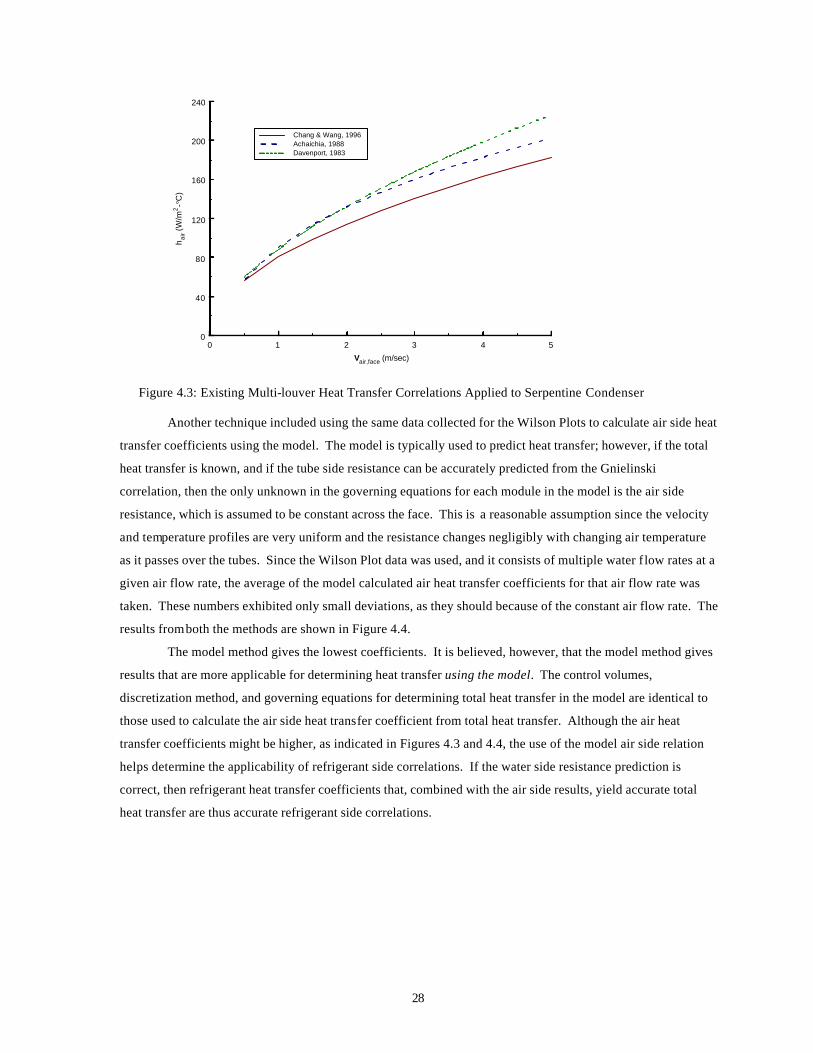
4.1.2 Air Side Heat Transfer The results from Chang & Wang, Davenport, and Achaichia’s correlations for local heat transfer
coefficients over multi-louvered fins were computed for the serpentine condenser’s fin geometry. These are
shown in Figure 4.3.
Air side heat transfer coefficients were experimentally determined using several techniques. One of
the techniques included the Wilson Plot. Cold water was run through the condenser at multiple flow rates in the
turbulent regime for given air flow rates. Total heat transfer was measured, and condenser resistance was
determined using an ε-NTU correlation for unmixed-unmixed cross-flow. A more detailed description of the
Wilson Plot technique and the slope plots for the serpentine condenser are given in Appendix C.
28
0 1 2 3 4 5
Vair,face (m/sec)
0
40
80
120
160
200
240
h air (
W/m
2-°
C)
Chang & Wang, 1996Achaichia, 1988Davenport, 1983
Figure 4.3: Existing Multi-louver Heat Transfer Correlations Applied to Serpentine Condenser
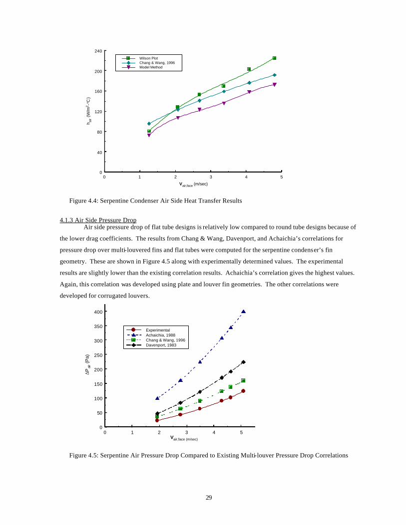
Another technique included using the same data collected for the Wilson Plots to calculate air side heat
transfer coefficients using the model. The model is typically used to predict heat transfer; however, if the total
heat transfer is known, and if the tube side resistance can be accurately predicted from the Gnielinski
correlation, then the only unknown in the governing equations for each module in the model is the air side
resistance, which is assumed to be constant across the face. This is a reasonable assumption since the velocity
and temperature profiles are very uniform and the resistance changes negligibly with changing air temperature
as it passes over the tubes. Since the Wilson Plot data was used, and it consists of multiple water f low rates at a
given air flow rate, the average of the model calculated air heat transfer coefficients for that air flow rate was
taken. These numbers exhibited only small deviations, as they should because of the constant air flow rate. The
results from both the methods are shown in Figure 4.4.
The model method gives the lowest coefficients. It is believed, however, that the model method gives
results that are more applicable for determining heat transfer using the model. The control volumes,
discretization method, and governing equations for determining total heat transfer in the model are identical to
those used to calculate the air side heat transfer coefficient from total heat transfer. Although the air heat
transfer coefficients might be higher, as indicated in Figures 4.3 and 4.4, the use of the model air side relation
helps determine the applicability of refrigerant side correlations. If the water side resistance prediction is
correct, then refrigerant heat transfer coefficients that, combined with the air side results, yield accurate total
heat transfer are thus accurate refrigerant side correlations.
29
0 1 2 3 4 5
Vair,face (m/sec)
0
40
80
120
160
200
240
h air (
W/m
2-°
C)
Wilson PlotChang & Wang, 1996Model Method
Figure 4.4: Serpentine Condenser Air Side Heat Transfer Results
4.1.3 Air Side Pressure Drop Air side pressure drop of flat tube designs is relatively low compared to round tube designs because of
the lower drag coefficients. The results from Chang & Wang, Davenport, and Achaichia’s correlations for
pressure drop over multi-louvered fins and flat tubes were computed for the serpentine condenser’s fin
geometry. These are shown in Figure 4.5 along with experimentally determined values. The experimental
results are slightly lower than the existing correlation results. Achaichia’s correlation gives the highest values.
Again, this correlation was developed using plate and louver fin geometries. The other correlations were
developed for corrugated louvers.
0 1 2 3 4 5Vair,face (m/sec)
0
50
100
150
200
250
300
350
400
∆P
air (
Pa)
ExperimentalAchaichia, 1988Chang & Wang, 1996Davenport, 1983
Figure 4.5: Serpentine Air Pressure Drop Compared to Existing Multi-louver Pressure Drop Correlations
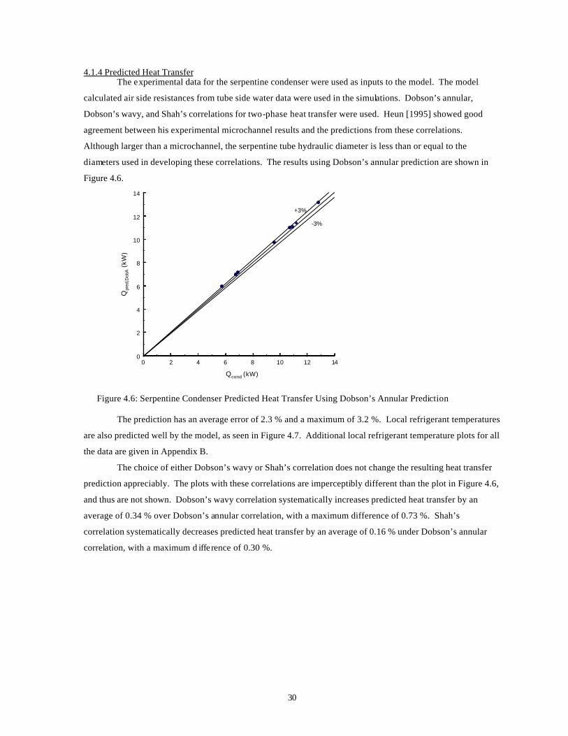
30
4.1.4 Predicted Heat Transfer The experimental data for the serpentine condenser were used as inputs to the model. The model
calculated air side resistances from tube side water data were used in the simulations. Dobson’s annular,
Dobson’s wavy, and Shah’s correlations for two-phase heat transfer were used. Heun [1995] showed good
agreement between his experimental microchannel results and the predictions from these correlations.
Although larger than a microchannel, the serpentine tube hydraulic diameter is less than or equal to the
diameters used in developing these correlations. The results using Dobson’s annular prediction are shown in
Figure 4.6.
0 2 4 6 8 10 12 14
Qcond (kW)
0
2
4
6
8
10
12
14
Qpr
ed,D
obA
(kW
)
+3%
-3%
Figure 4.6: Serpentine Condenser Predicted Heat Transfer Using Dobson’s Annular Prediction
The prediction has an average error of 2.3 % and a maximum of 3.2 %. Local refrigerant temperatures
are also predicted well by the model, as seen in Figure 4.7. Additional local refrigerant temperature plots for all
the data are given in Appendix B.
The choice of either Dobson’s wavy or Shah’s correlation does not change the resulting heat transfer
prediction appreciably. The plots with these correlations are imperceptibly different than the plot in Figure 4.6,
and thus are not shown. Dobson’s wavy correlation systematically increases predicted heat transfer by an
average of 0.34 % over Dobson’s annular correlation, with a maximum difference of 0.73 %. Shah’s
correlation systematically decreases predicted heat transfer by an average of 0.16 % under Dobson’s annular
correlation, with a maximum d iffe rence of 0.30 %.
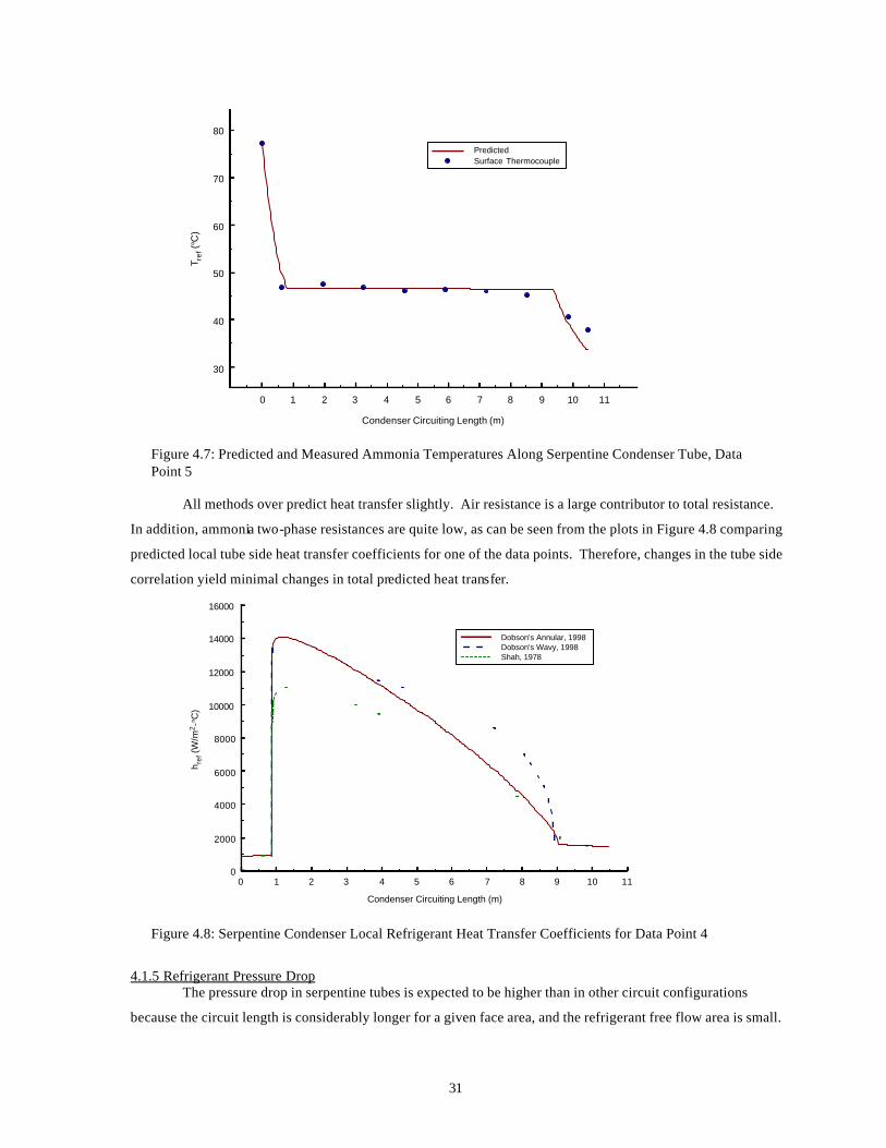
31
0 1 2 3 4 5 6 7 8 9 10 11
Condenser Circuiting Length (m)
30
40
50
60
70
80
T ref (
°C)
PredictedSurface Thermocouple
Figure 4.7: Predicted and Measured Ammonia Temperatures Along Serpentine Condenser Tube, Data Point 5
All methods over predict heat transfer slightly. Air resistance is a large contributor to total resistance.
In addition, ammonia two-phase resistances are quite low, as can be seen from the plots in Figure 4.8 comparing
predicted local tube side heat transfer coefficients for one of the data points. Therefore, changes in the tube side
correlation yield minimal changes in total predicted heat transfer.
0 1 2 3 4 5 6 7 8 9 10 11
Condenser Circuiting Length (m)
0
2000
4000
6000
8000
10000
12000
14000
16000
h ref (
W/m
2-°
C)
Dobson's Annular, 1998Dobson's Wavy, 1998Shah, 1978
Figure 4.8: Serpentine Condenser Local Refrigerant Heat Transfer Coefficients for Data Point 4
4.1.5 Refrigerant Pressure Drop The pressure drop in serpentine tubes is expected to be higher than in other circuit configurations
because the circuit length is considerably longer for a given face area, and the refrigerant free flow area is small.
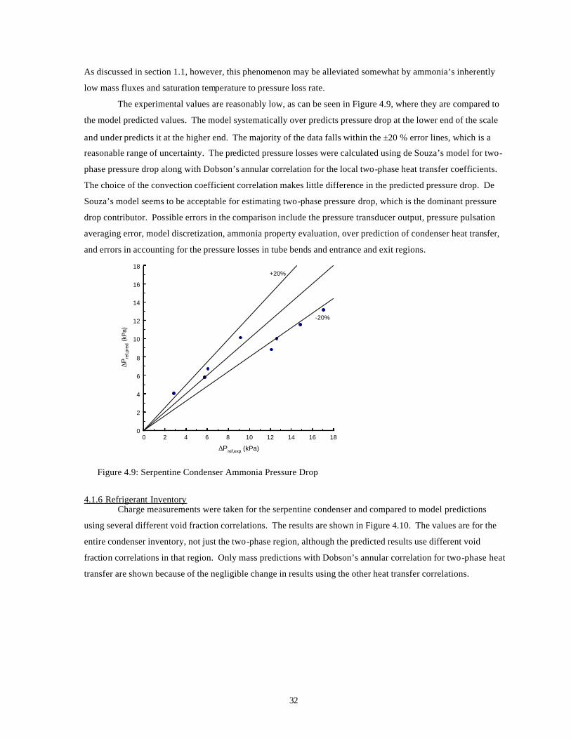
32
As discussed in section 1.1, however, this phenomenon may be alleviated somewhat by ammonia’s inherently
low mass fluxes and saturation temperature to pressure loss rate.
The experimental values are reasonably low, as can be seen in Figure 4.9, where they are compared to
the model predicted values. The model systematically over predicts pressure drop at the lower end of the scale
and under predicts it at the higher end. The majority of the data falls within the ±20 % error lines, which is a
reasonable range of uncertainty. The predicted pressure losses were calculated using de Souza’s model for two-
phase pressure drop along with Dobson’s annular correlation for the local two-phase heat transfer coefficients.
The choice of the convection coefficient correlation makes little difference in the predicted pressure drop. De
Souza’s model seems to be acceptable for estimating two-phase pressure drop, which is the dominant pressure
drop contributor. Possible errors in the comparison include the pressure transducer output, pressure pulsation
averaging error, model discretization, ammonia property evaluation, over prediction of condenser heat transfer,
and errors in accounting for the pressure losses in tube bends and entrance and exit regions.
0 2 4 6 8 10 12 14 16 18
∆Pref,exp (kPa)
0
2
4
6
8
10
12
14
16
18
∆P
ref,p
red (k
Pa)
+20%
-20%
Figure 4.9: Serpentine Condenser Ammonia Pressure Drop
4.1.6 Refrigerant Inventory Charge measurements were taken for the serpentine condenser and compared to model predictions
using several different void fraction correlations. The results are shown in Figure 4.10. The values are for the
entire condenser inventory, not just the two-phase region, although the predicted results use different void
fraction correlations in that region. Only mass predictions with Dobson’s annular correlation for two-phase heat
transfer are shown because of the negligible change in results using the other heat transfer correlations.
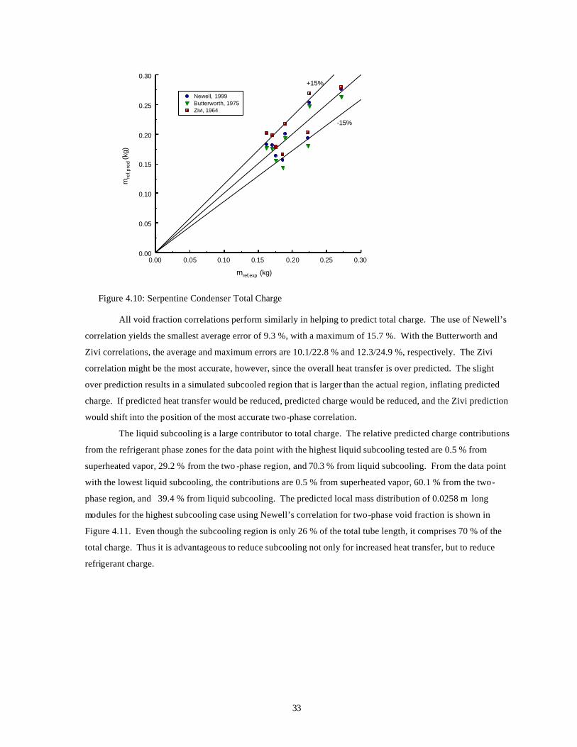
33
0.00 0.05 0.10 0.15 0.20 0.25 0.30
mref,exp (kg)
0.00
0.05
0.10
0.15
0.20
0.25
0.30
mre
f,pre
d (kg
)
+15%
-15%
Newell, 1999Butterworth, 1975Zivi, 1964
Figure 4.10: Serpentine Condenser Total Charge
All void fraction correlations perform similarly in helping to predict total charge. The use of Newell’s
correlation yields the smallest average error of 9.3 %, with a maximum of 15.7 %. With the Butterworth and
Zivi correlations, the average and maximum errors are 10.1/22.8 % and 12.3/24.9 %, respectively. The Zivi
correlation might be the most accurate, however, since the overall heat transfer is over predicted. The slight
over prediction results in a simulated subcooled region that is larger than the actual region, inflating predicted
charge. If predicted heat transfer would be reduced, predicted charge would be reduced, and the Zivi prediction
would shift into the position of the most accurate two-phase correlation.
The liquid subcooling is a large contributor to total charge. The relative predicted charge contributions
from the refrigerant phase zones for the data point with the highest liquid subcooling tested are 0.5 % from
superheated vapor, 29.2 % from the two -phase region, and 70.3 % from liquid subcooling. From the data point
with the lowest liquid subcooling, the contributions are 0.5 % from superheated vapor, 60.1 % from the two-
phase region, and 39.4 % from liquid subcooling. The predicted local mass distribution of 0.0258 m long
modules for the highest subcooling case using Newell’s correlation for two-phase void fraction is shown in
Figure 4.11. Even though the subcooling region is only 26 % of the total tube length, it comprises 70 % of the
total charge. Thus it is advantageous to reduce subcooling not only for increased heat transfer, but to reduce
refrigerant charge.
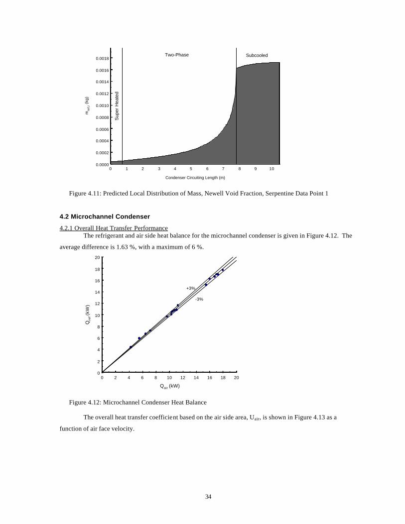
34
0 1 2 3 4 5 6 7 8 9 10
Condenser Circuiting Length (m)
0.0000
0.0002
0.0004
0.0006
0.0008
0.0010
0.0012
0.0014
0.0016
0.0018
mre
f,i (
kg)
Two-Phase
Sup
er H
eate
d
Subcooled
Figure 4.11: Predicted Local Distribution of Mass, Newell Void Fraction, Serpentine Data Point 1
4.2 Microchannel Condenser
4.2.1 Overall Heat Transfer Performance The refrigerant and air side heat balance for the microchannel condenser is given in Figure 4.12. The
average difference is 1.63 %, with a maximum of 6 %.
0 2 4 6 8 10 12 14 16 18 20
Qair (kW)
0
2
4
6
8
10
12
14
16
18
20
Qre
f (kW
)
+3%
-3%
Figure 4.12: Microchannel Condenser Heat Balance
The overall heat transfer coefficient based on the air side area, Uair, is shown in Figure 4.13 as a
function of air face velocity.
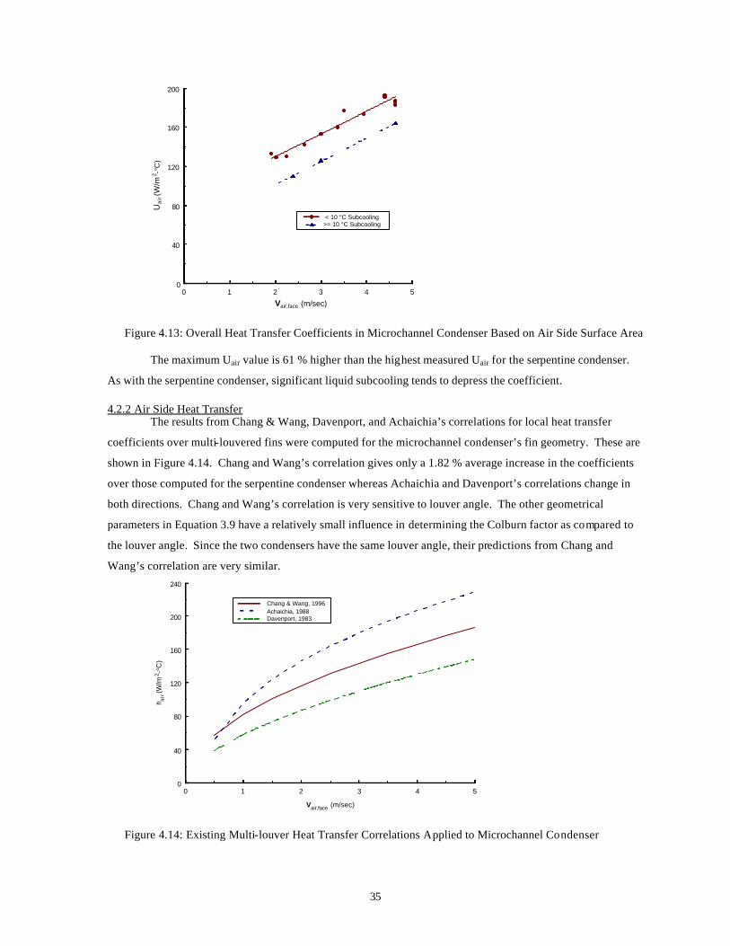
35
0 1 2 3 4 5
Vair,face (m/sec)
0
40
80
120
160
200
Ua
ir (W
/m2 -°
C)
< 10 °C Subcooling>= 10 °C Subcooling
Figure 4.13: Overall Heat Transfer Coefficients in Microchannel Condenser Based on Air Side Surface Area
The maximum Uair value is 61 % higher than the highest measured Uair for the serpentine condenser.
As with the serpentine condenser, significant liquid subcooling tends to depress the coefficient.
4.2.2 Air Side Heat Transfer The results from Chang & Wang, Davenport, and Achaichia’s correlations for local heat transfer
coefficients over multi-louvered fins were computed for the microchannel condenser’s fin geometry. These are
shown in Figure 4.14. Chang and Wang’s correlation gives only a 1.82 % average increase in the coefficients
over those computed for the serpentine condenser whereas Achaichia and Davenport’s correlations change in
both directions. Chang and Wang’s correlation is very sensitive to louver angle. The other geometrical
parameters in Equation 3.9 have a relatively small influence in determining the Colburn factor as compared to
the louver angle. Since the two condensers have the same louver angle, their predictions from Chang and
Wang’s correlation are very similar.
0 1 2 3 4 5
Vair,face (m/sec)
0
40
80
120
160
200
240
h air
(W/m
2 -°C
)
Chang & Wang, 1996Achaichia, 1988Davenport, 1983
Figure 4.14: Existing Multi-louver Heat Transfer Correlations Applied to Microchannel Condenser
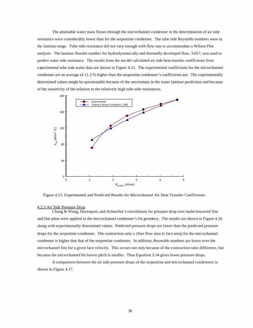
36
The attainable water mass fluxes through the microchannel condenser in the determination of air side
resistance were considerably lower than for the serpentine condenser. The tube side Reynolds numbers were in
the laminar range. Tube side resistance did not vary enough with flow rate to accommodate a Wilson Plot
analysis. The laminar Nusslet number for hydrodynamically and thermally developed flow, 3.657, was used to
predict water side resistance. The results from the mo del calculated air side heat transfer coefficients from
experimental tube side water data are shown in Figure 4.15. The experimental coefficients for the microchannel
condenser are an average of 11.2 % higher than the serpentine condenser’s coefficients are. The experimentally
determined values might be questionable because of the uncertainty in the water laminar prediction and because
of the sensitivity of the solution to the relatively high tube side resistances.
0 1 2 3 4 5
Vair,face (m/sec)
0
40
80
120
160
200
h air
(W/m
2 -°C
)
ExperimentalChang & Wang Correlation, 1996
Figure 4.15: Experimental and Predicted Results for Microchannel Air Heat Transfer Coefficients
4.2.3 Air Side Pressure Drop Chang & Wang, Davenport, and Achaichia’s correlations for pressure drop over multi-louvered fins
and flat tubes were applied to the microchannel condenser’s fin geometry. The results are shown in Figure 4.16
along with experimentally determined values. Predicted pressure drops are lower than the predicted pressure
drops for the serpentine condenser. The contraction ratio σ (free flow area to face area) for the microchannel
condenser is higher that that of the serpentine condenser. In addition, Reynolds numbers are lower over the
microchannel fins for a given face velocity. This occurs not only because of the contraction ratio difference, but
because the microchannel fin louver pitch is smaller. Thus Equation 3.34 gives lower pressure drops.
A comparison between the air side pressure drops of the serpentine and microchannel condensers is
shown in Figure 4.17.
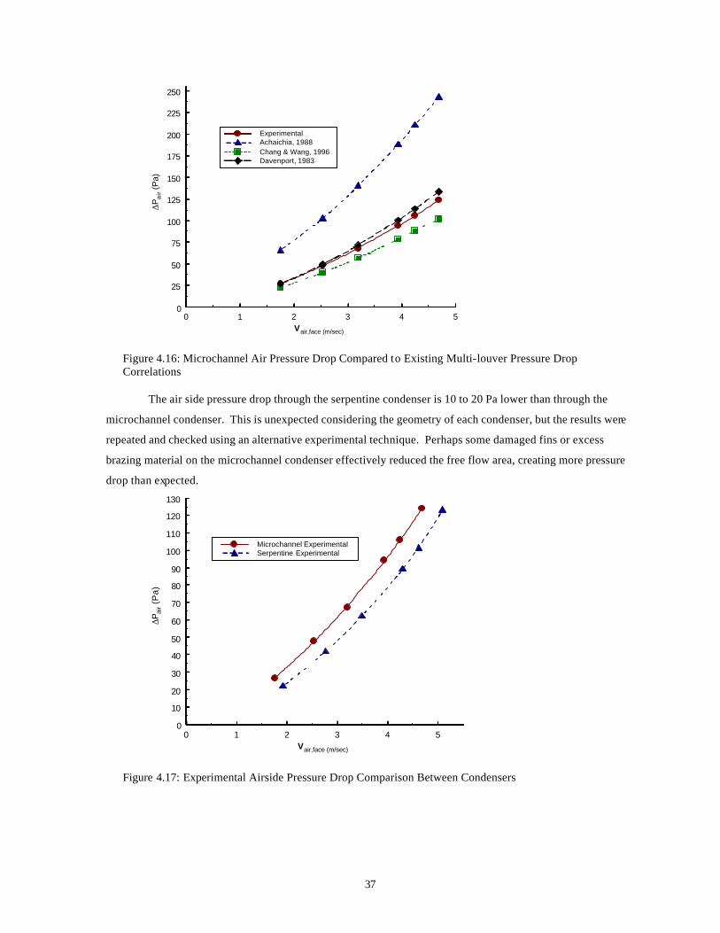
37
0 1 2 3 4 5Vair,face (m/sec)
0
25
50
75
100
125
150
175
200
225
250
∆P
air (
Pa)
ExperimentalAchaichia, 1988Chang & Wang, 1996Davenport, 1983
Figure 4.16: Microchannel Air Pressure Drop Compared to Existing Multi-louver Pressure Drop Correlations
The air side pressure drop through the serpentine condenser is 10 to 20 Pa lower than through the
microchannel condenser. This is unexpected considering the geometry of each condenser, but the results were
repeated and checked using an alternative experimental technique. Perhaps some damaged fins or excess
brazing material on the microchannel condenser effectively reduced the free flow area, creating more pressure
drop than expected.
0 1 2 3 4 5Vair,face (m/sec)
0
10
20
30
40
50
60
70
80
90
100
110
120
130
∆Pai
r (P
a)
Microchannel ExperimentalSerpentine Experimental
Figure 4.17: Experimental Airside Pressure Drop Comparison Between Condensers
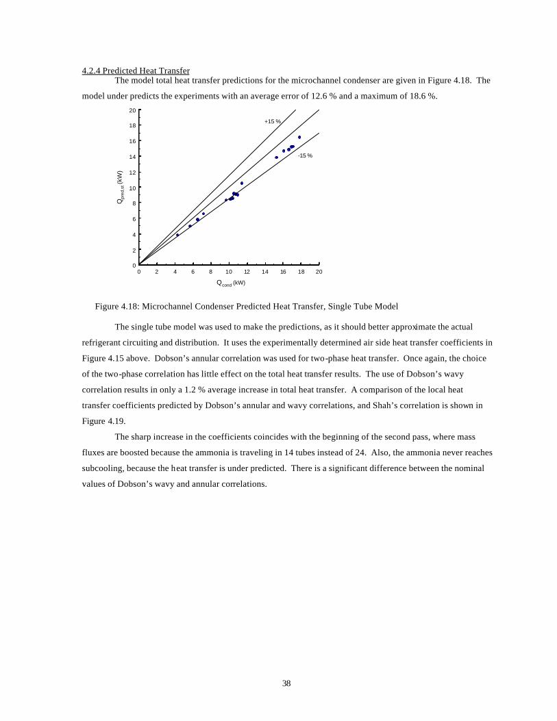
38
4.2.4 Predicted Heat Transfer The model total heat transfer predictions for the microchannel condenser are given in Figure 4.18. The
model under predicts the experiments with an average error of 12.6 % and a maximum of 18.6 %.
0 2 4 6 8 10 12 14 16 18 20
Qcond (kW)
0
2
4
6
8
10
12
14
16
18
20
Qpr
ed,s
t (kW
)+15 %
-15 %
Figure 4.18: Microchannel Condenser Predicted Heat Transfer, Single Tube Model
The single tube model was used to make the predictions, as it should better approximate the actual
refrigerant circuiting and distribution. It uses the experimentally determined air side heat transfer coefficients in
Figure 4.15 above. Dobson’s annular correlation was used for two-phase heat transfer. Once again, the choice
of the two-phase correlation has little effect on the total heat transfer results. The use of Dobson’s wavy
correlation results in only a 1.2 % average increase in total heat transfer. A comparison of the local heat
transfer coefficients predicted by Dobson’s annular and wavy correlations, and Shah’s correlation is shown in
Figure 4.19.
The sharp increase in the coefficients coincides with the beginning of the second pass, where mass
fluxes are boosted because the ammonia is traveling in 14 tubes instead of 24. Also, the ammonia never reaches
subcooling, because the heat transfer is under predicted. There is a significant difference between the nominal
values of Dobson’s wavy and annular correlations.
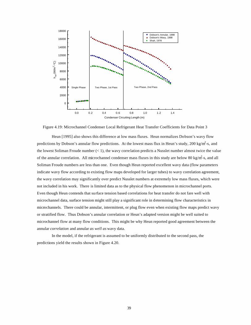
39
0.0 0.2 0.4 0.6 0.8 1.0 1.2 1.4
Condenser Circuiting Length (m)
0
2000
4000
6000
8000
10000
12000
14000
16000
18000
h ref (
W/m
2 -°C
)
Dobson's Annular, 1998Dobson's Wavy, 1998Shah, 1978
Single Phase Two Phase, 1st Pass Two Phase, 2nd Pass
Figure 4.19: Microchannel Condenser Local Refrigerant Heat Transfer Coefficients for Data Point 3
Heun [1995] also shows this difference at low mass fluxes. Heun normalizes Dobson’s wavy flow
predictions by Dobson’s annular flow predictions. At the lowest mass flux in Heun’s study, 200 kg/m2-s, and
the lowest Soliman Froude number (< 1), the wavy correlation predicts a Nusslet number almost twice the value
of the annular correlation. All microchannel condenser mass fluxes in this study are below 80 kg/m2-s, and all
Soliman Froude numbers are less than one. Even though Heun reported excellent wavy data (flow parameters
indicate wavy flow according to existing flow maps developed for larger tubes) to wavy correlation agreement,
the wavy correlation may significantly over predict Nusslet numbers at extremely low mass fluxes, which were
not included in his work. There is limited data as to the physical flow phenomenon in microchannel ports.
Even though Heun contends that surface tension based correlations for heat transfer do not fare well with
microchannel data, surface tension might still play a significant role in determining flow characteristics in
microchannels. There could be annular, intermittent, or plug flow even when existing flow maps predict wavy
or stratified flow. Thus Dobson’s annular correlation or Heun’s adapted version might be well suited to
microchannel flow at many flow conditions. This might be why Heun reported good agreement between the
annular correlation and annular as well as wavy data.
In the model, if the refrigerant is assumed to be uniformly distributed to the second pass, the
predictions yield the results shown in Figure 4.20.
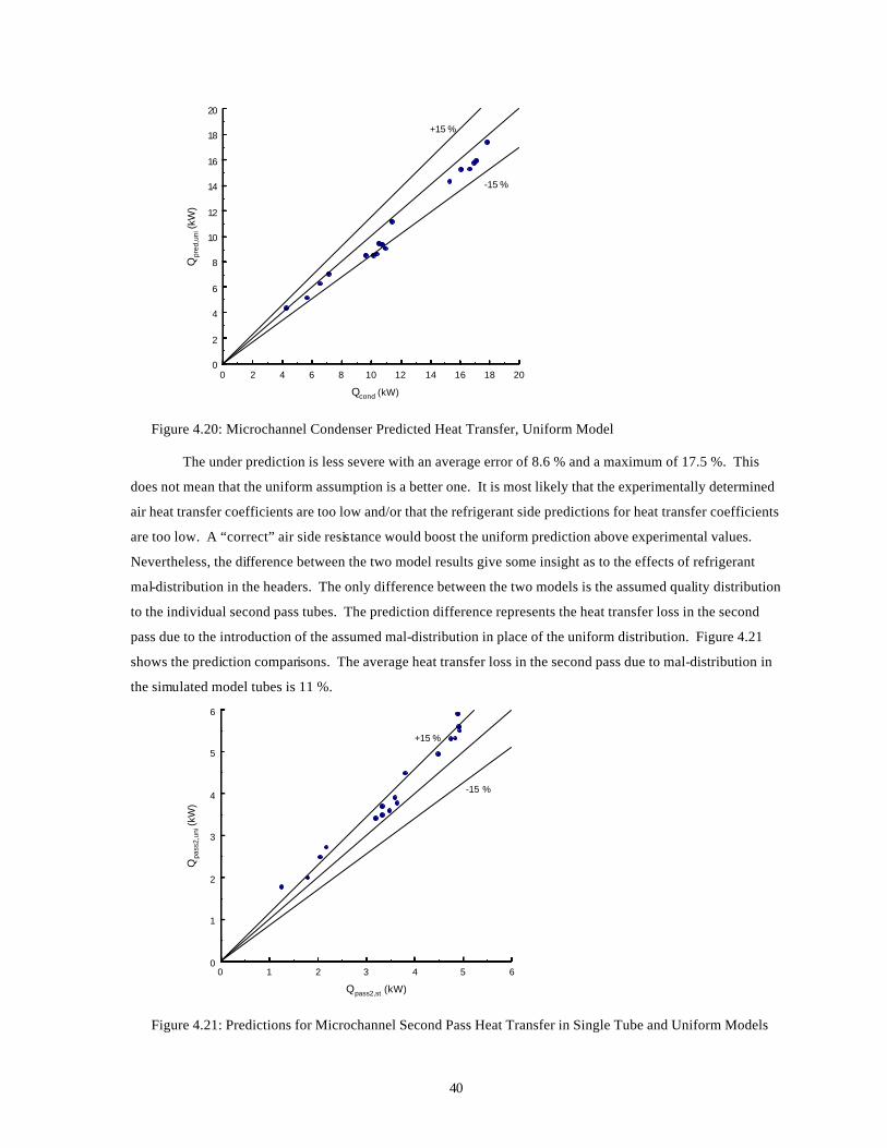
40
0 2 4 6 8 10 12 14 16 18 20
Qcond (kW)
0
2
4
6
8
10
12
14
16
18
20
Qpr
ed,u
ni (
kW)
+15 %
-15 %
Figure 4.20: Microchannel Condenser Predicted Heat Transfer, Uniform Model
The under prediction is less severe with an average error of 8.6 % and a maximum of 17.5 %. This
does not mean that the uniform assumption is a better one. It is most likely that the experimentally determined
air heat transfer coefficients are too low and/or that the refrigerant side predictions for heat transfer coefficients
are too low. A “correct” air side resistance would boost the uniform prediction above experimental values.
Nevertheless, the difference between the two model results give some insight as to the effects of refrigerant
mal-distribution in the headers. The only difference between the two models is the assumed quality distribution
to the individual second pass tubes. The prediction difference represents the heat transfer loss in the second
pass due to the introduction of the assumed mal-distribution in place of the uniform distribution. Figure 4.21
shows the prediction comparisons. The average heat transfer loss in the second pass due to mal-distribution in
the simulated model tubes is 11 %.
0 1 2 3 4 5 6
Qpass2,st (kW)
0
1
2
3
4
5
6
Qpa
ss2,
uni (
kW)
+15 %
-15 %
Figure 4.21: Predictions for Microchannel Second Pass Heat Transfer in Single Tube and Uniform Models
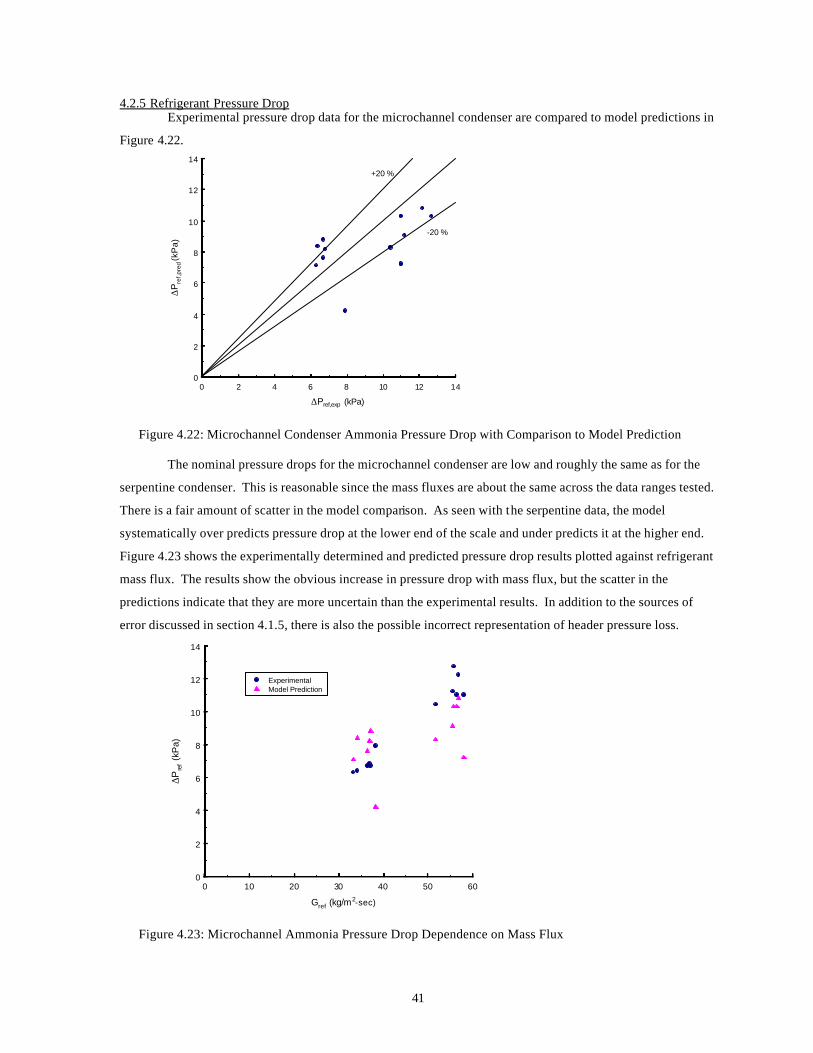
41
4.2.5 Refrigerant Pressure Drop Experimental pressure drop data for the microchannel condenser are compared to model predictions in
Figure 4.22.
0 2 4 6 8 10 12 14
∆Pref,exp (kPa)
0
2
4
6
8
10
12
14
∆P
ref,p
red (
kPa)
+20 %
-20 %
Figure 4.22: Microchannel Condenser Ammonia Pressure Drop with Comparison to Model Prediction
The nominal pressure drops for the microchannel condenser are low and roughly the same as for the
serpentine condenser. This is reasonable since the mass fluxes are about the same across the data ranges tested.
There is a fair amount of scatter in the model comparison. As seen with the serpentine data, the model
systematically over predicts pressure drop at the lower end of the scale and under predicts it at the higher end.
Figure 4.23 shows the experimentally determined and predicted pressure drop results plotted against refrigerant
mass flux. The results show the obvious increase in pressure drop with mass flux, but the scatter in the
predictions indicate that they are more uncertain than the experimental results. In addition to the sources of
error discussed in section 4.1.5, there is also the possible incorrect representation of header pressure loss.
0 10 20 30 40 50 60
Gref (kg/m2-sec)
0
2
4
6
8
10
12
14
∆Pre
f (kP
a)
ExperimentalModel Prediction
Figure 4.23: Microchannel Ammonia Pressure Drop Dependence on Mass Flux
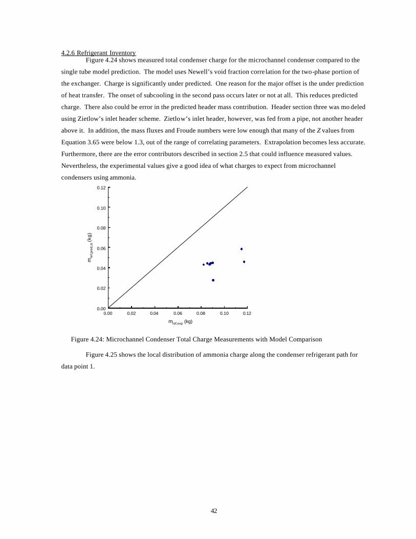
42
4.2.6 Refrigerant Inventory Figure 4.24 shows measured total condenser charge for the microchannel condenser compared to the
single tube model prediction. The model uses Newell’s void fraction correlation for the two-phase portion of
the exchanger. Charge is significantly under predicted. One reason for the major offset is the under prediction
of heat transfer. The onset of subcooling in the second pass occurs later or not at all. This reduces predicted
charge. There also could be error in the predicted header mass contribution. Header section three was mo deled
using Zietlow’s inlet header scheme. Zietlow’s inlet header, however, was fed from a pipe, not another header
above it. In addition, the mass fluxes and Froude numbers were low enough that many of the Z values from
Equation 3.65 were below 1.3, out of the range of correlating parameters. Extrapolation becomes less accurate.
Furthermore, there are the error contributors described in section 2.5 that could influence measured values.
Nevertheless, the experimental values give a good idea of what charges to expect from microchannel
condensers using ammonia.
0.00 0.02 0.04 0.06 0.08 0.10 0.12
mref,exp (kg)
0.00
0.02
0.04
0.06
0.08
0.10
0.12
mre
f,pre
d,st (k
g)
Figure 4.24: Microchannel Condenser Total Charge Measurements with Model Comparison
Figure 4.25 shows the local distribution of ammonia charge along the condenser refrigerant path for
data point 1.
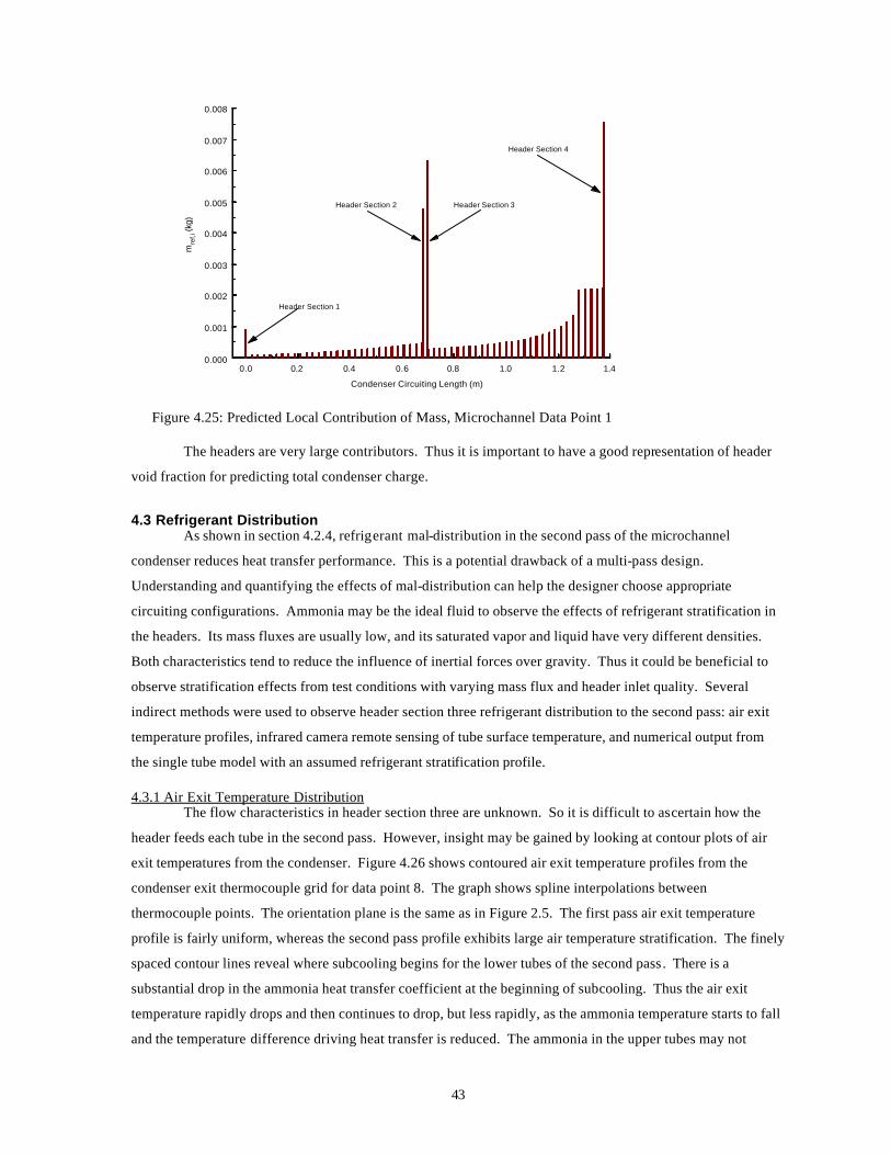
43
0.0 0.2 0.4 0.6 0.8 1.0 1.2 1.4
Condenser Circuiting Length (m)
0.000
0.001
0.002
0.003
0.004
0.005
0.006
0.007
0.008
mre
f,i (k
g)
Header Section 1
Header Section 2 Header Section 3
Header Section 4
Figure 4.25: Predicted Local Contribution of Mass, Microchannel Data Point 1
The headers are very large contributors. Thus it is important to have a good representation of header
void fraction for predicting total condenser charge.
4.3 Refrigerant Distribution As shown in section 4.2.4, refrigerant mal-distribution in the second pass of the microchannel
condenser reduces heat transfer performance. This is a potential drawback of a multi-pass design.
Understanding and quantifying the effects of mal-distribution can help the designer choose appropriate
circuiting configurations. Ammonia may be the ideal fluid to observe the effects of refrigerant stratification in
the headers. Its mass fluxes are usually low, and its saturated vapor and liquid have very different densities.
Both characteristics tend to reduce the influence of inertial forces over gravity. Thus it could be beneficial to
observe stratification effects from test conditions with varying mass flux and header inlet quality. Several
indirect methods were used to observe header section three refrigerant distribution to the second pass: air exit
temperature profiles, infrared camera remote sensing of tube surface temperature, and numerical output from
the single tube model with an assumed refrigerant stratification profile.
4.3.1 Air Exit Temperature Distribution The flow characteristics in header section three are unknown. So it is difficult to ascertain how the
header feeds each tube in the second pass. However, insight may be gained by looking at contour plots of air
exit temperatures from the condenser. Figure 4.26 shows contoured air exit temperature profiles from the
condenser exit thermocouple grid for data point 8. The graph shows spline interpolations between
thermocouple points. The orientation plane is the same as in Figure 2.5. The first pass air exit temperature
profile is fairly uniform, whereas the second pass profile exhibits large air temperature stratification. The finely
spaced contour lines reveal where subcooling begins for the lower tubes of the second pass. There is a
substantial drop in the ammonia heat transfer coefficient at the beginning of subcooling. Thus the air exit
temperature rapidly drops and then continues to drop, but less rapidly, as the ammonia temperature starts to fall
and the temperature difference driving heat transfer is reduced. The ammonia in the upper tubes may not
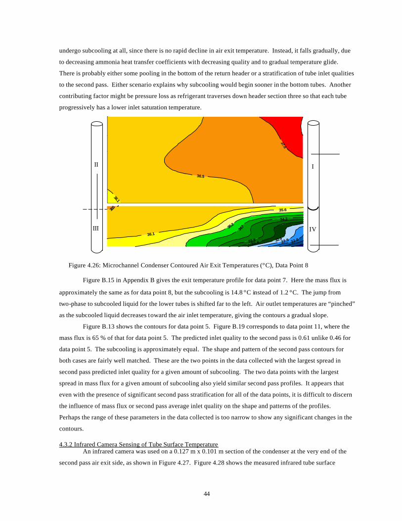
44
undergo subcooling at all, since there is no rapid decline in air exit temperature. Instead, it falls gradually, due
to decreasing ammonia heat transfer coefficients with decreasing quality and to gradual temperature glide.
There is probably either some pooling in the bottom of the return header or a stratification of tube inlet qualities
to the second pass. Either scenario explains why subcooling would begin sooner in the bottom tubes. Another
contributing factor might be pressure loss as refrigerant traverses down header section three so that each tube
progressively has a lower inlet saturation temperature.
Figure 4.26: Microchannel Condenser Contoured Air Exit Temperatures (°C), Data Point 8
Figure B.15 in Appendix B gives the exit temperature profile for data point 7. Here the mass flux is
approximately the same as for data point 8, but the subcooling is 14.8 °C instead of 1.2 °C. The jump from
two-phase to subcooled liquid for the lower tubes is shifted far to the left. Air outlet temperatures are “pinched”
as the subcooled liquid decreases toward the air inlet temperature, giving the contours a gradual slope.
Figure B.13 shows the contours for data point 5. Figure B.19 corresponds to data point 11, where the
mass flux is 65 % of that for data point 5. The predicted inlet quality to the second pass is 0.61 unlike 0.46 for
data point 5. The subcooling is approximately equal. The shape and pattern of the second pass contours for
both cases are fairly well matched. These are the two points in the data collected with the largest spread in
second pass predicted inlet quality for a given amount of subcooling. The two data points with the largest
spread in mass flux for a given amount of subcooling also yield similar second pass profiles. It appears that
even with the presence of significant second pass stratification for all of the data points, it is difficult to discern
the influence of mass flux or second pass average inlet quality on the shape and patterns of the profiles.
Perhaps the range of these parameters in the data collected is too narrow to show any significant changes in the
contours.
4.3.2 Infrared Camera Sensing of Tube Surface Temperature An infrared camera was used on a 0.127 m x 0.101 m section of the condenser at the very end of the
second pass air exit side, as shown in Figure 4.27. Figure 4.28 shows the measured infrared tube surface
II I
III IV
32.0 32.5 32.9 33.4 33.8
34.3
34.7 35
.2
35.6
36.1
36.5
36.1
36.5
37.0
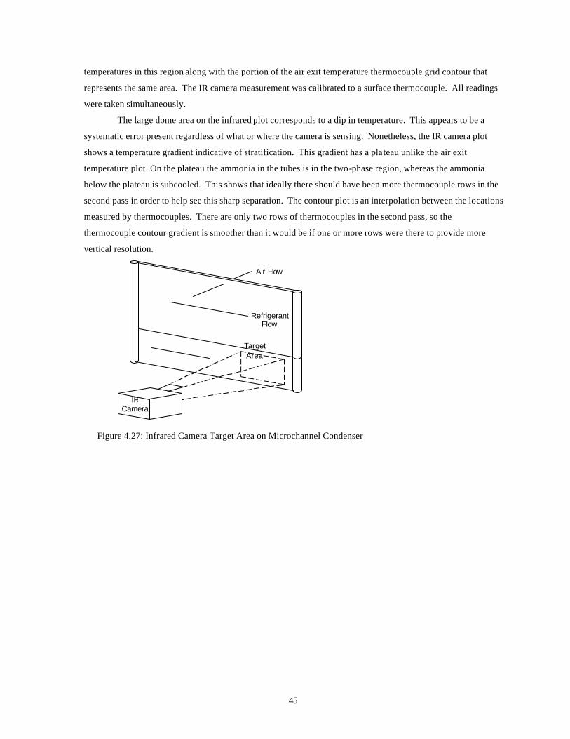
45
temperatures in this region along with the portion of the air exit temperature thermocouple grid contour that
represents the same area. The IR camera measurement was calibrated to a surface thermocouple. All readings
were taken simultaneously.
The large dome area on the infrared plot corresponds to a dip in temperature. This appears to be a
systematic error present regardless of what or where the camera is sensing. Nonetheless, the IR camera plot
shows a temperature gradient indicative of stratification. This gradient has a plateau unlike the air exit
temperature plot. On the plateau the ammonia in the tubes is in the two-phase region, whereas the ammonia
below the plateau is subcooled. This shows that ideally there should have been more thermocouple rows in the
second pass in order to help see this sharp separation. The contour plot is an interpolation between the locations
measured by thermocouples. There are only two rows of thermocouples in the second pass, so the
thermocouple contour gradient is smoother than it would be if one or more rows were there to provide more
vertical resolution.
Figure 4.27: Infrared Camera Target Area on Microchannel Condenser
Air Flow
Refrigerant Flow
IR Camera
Target Area

46
33.0
33.6 34.2 34.7 35.3
35.9
35.9
Tube Surface Temperature (°C) from IR Camera
30.1 30.6
31.2
31.8
32.3 32.9
33.4
Air Exit Temperature (°C) from Thermocouple Grid
Figure 4.28: Infrared Camera Contour of Target Area with Corresponding Air Outlet Temperature Contour; Conditions Correspond to Microchannel Data Point 12
Figure 4.29 shows temperature plots for the tube that runs along the level of the bottom thermocouple
row (this corresponds to a profile along the bottom edge of Figure 4.28).
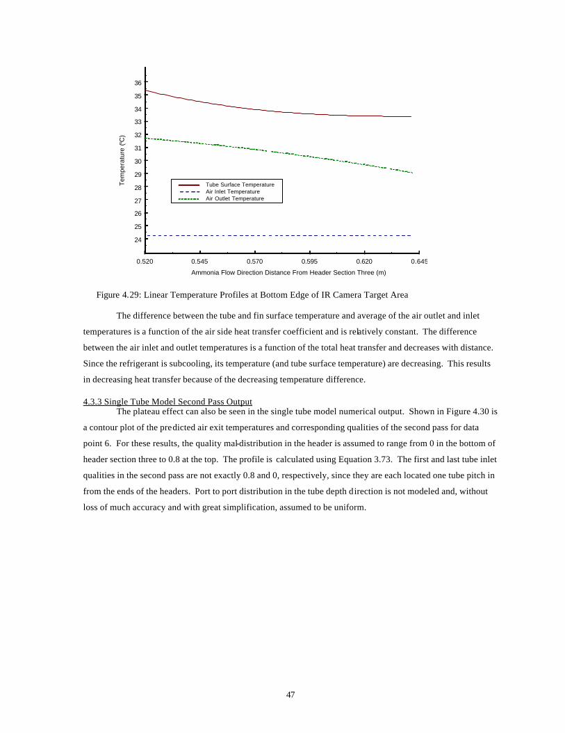
47
0.520 0.545 0.570 0.595 0.620 0.645
Ammonia Flow Direction Distance From Header Section Three (m)
24
25
26
27
28
29
30
31
32
33
34
35
36
Tem
pera
ture
(°C
)
Tube Surface TemperatureAir Inlet TemperatureAir Outlet Temperature
Figure 4.29: Linear Temperature Profiles at Bottom Edge of IR Camera Target Area
The difference between the tube and fin surface temperature and average of the air outlet and inlet
temperatures is a function of the air side heat transfer coefficient and is relatively constant. The difference
between the air inlet and outlet temperatures is a function of the total heat transfer and decreases with distance.
Since the refrigerant is subcooling, its temperature (and tube surface temperature) are decreasing. This results
in decreasing heat transfer because of the decreasing temperature difference.
4.3.3 Single Tube Model Second Pass Output The plateau effect can also be seen in the single tube model numerical output. Shown in Figure 4.30 is
a contour plot of the predicted air exit temperatures and corresponding qualities of the second pass for data
point 6. For these results, the quality mal-distribution in the header is assumed to range from 0 in the bottom of
header section three to 0.8 at the top. The profile is calculated using Equation 3.73. The first and last tube inlet
qualities in the second pass are not exactly 0.8 and 0, respectively, since they are each located one tube pitch in
from the ends of the headers. Port to port distribution in the tube depth direction is not modeled and, without
loss of much accuracy and with great simplification, assumed to be uniform.
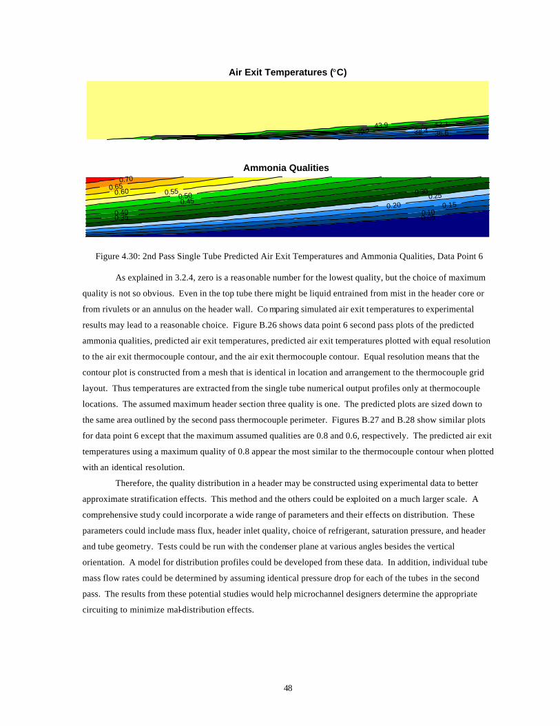
48
36.6 38.4 40.2 42.1 43.9
Air Exit Temperatures (°C)
Ammonia Qualities
0.05 0.10 0.15 0.20
0.25 0.30
0.35 0.40 0.45 0.50 0.55 0.60 0.65
0.70
Figure 4.30: 2nd Pass Single Tube Predicted Air Exit Temperatures and Ammonia Qualities, Data Point 6
As explained in 3.2.4, zero is a reasonable number for the lowest quality, but the choice of maximum
quality is not so obvious. Even in the top tube there might be liquid entrained from mist in the header core or
from rivulets or an annulus on the header wall. Co mparing simulated air exit temperatures to experimental
results may lead to a reasonable choice. Figure B.26 shows data point 6 second pass plots of the predicted
ammonia qualities, predicted air exit temperatures, predicted air exit temperatures plotted with equal resolution
to the air exit thermocouple contour, and the air exit thermocouple contour. Equal resolution means that the
contour plot is constructed from a mesh that is identical in location and arrangement to the thermocouple grid
layout. Thus temperatures are extracted from the single tube numerical output profiles only at thermocouple
locations. The assumed maximum header section three quality is one. The predicted plots are sized down to
the same area outlined by the second pass thermocouple perimeter. Figures B.27 and B.28 show similar plots
for data point 6 except that the maximum assumed qualities are 0.8 and 0.6, respectively. The predicted air exit
temperatures using a maximum quality of 0.8 appear the most similar to the thermocouple contour when plotted
with an identical resolution.
Therefore, the quality distribution in a header may be constructed using experimental data to better
approximate stratification effects. This method and the others could be exploited on a much larger scale. A
comprehensive study could incorporate a wide range of parameters and their effects on distribution. These
parameters could include mass flux, header inlet quality, choice of refrigerant, saturation pressure, and header
and tube geometry. Tests could be run with the condenser plane at various angles besides the vertical
orientation. A model for distribution profiles could be developed from these data. In addition, individual tube
mass flow rates could be determined by assuming identical pressure drop for each of the tubes in the second
pass. The results from these potential studies would help microchannel designers determine the appropriate
circuiting to minimize mal-distribution effects.
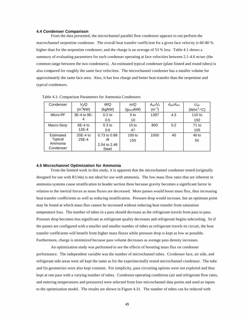
49
4.4 Condenser Comparison From the data presented, the microchannel parallel flow condenser appears to out perform the
macrochannel serpentine condenser. The overall heat transfer coefficient for a given face velocity is 60-80 %
higher than for the serpentine condenser; and the charge is an average of 53 % less. Table 4.1 shows a
summary of evaluating parameters for each condenser operating at face velocities between 2.1-4.6 m/sec (the
common range between the two condensers). An estimated typical condenser (plate finned and round tubes) is
also compared for roughly the same face velocities. The microchannel condenser has a smaller volume for
approximately the same face area. Also, it has less charge and better heat transfer than the serpentine and
typical condensers.
Table 4.1: Comparison Parameters for Ammonia Condensers
Condenser Ve/Q (m3/kW)
M/Q (kg/kW)
m/Q (gNH3/kW)
Aair/Ve (m -1)
Aair/Aref Uair (W/m2-°C)
Micro-PF 3E-4 to 9E-4
0.2 to 0.5
5 to 10
1397 4.3 110 to 192
Macro-Serp 6E-4 to 12E-4
0.3 to 0.6
15 to 47
800 5.2 71 to 105
Estimated Typical
Ammonia Condenser
20E-4 to 25E-4
0.73 to 0.88 Al
2.04 to 2.46 Steel
100 to 150
1000 40 40 to 50
4.5 Microchannel Optimization for Ammonia From the limited work in this study, it is apparent that the microchannel condenser tested (originally
designed for use with R134a) is not ideal for use with ammonia. The low mass flow rates that are inherent in
ammonia systems cause stratification in header section three because gravity becomes a significant factor in
relation to the inertial forces as mass fluxes are decreased. More passes would boost mass flux, thus increasing
heat transfer coefficients as well as reducing stratification. Pressure drop would increase, but an optimum point
may be found at which mass flux cannot be increased without reducing heat transfer from saturation
temperature loss. The number of tubes in a pass should decrease as the refrigerant travels from pass to pass.
Pressure drop becomes less significant as refrigerant quality decreases and refrigerant begins subcooling. So if
the passes are configured with a smaller and smaller number of tubes as refrigerant travels its circuit, the heat
transfer coefficients will benefit from higher mass fluxes while pressure drop is kept as low as possible.
Furthermore, charge is minimized because pass volume decreases as average pass density increases.
An optimization study was performed to see the effects of boosting mass flux on condenser
performance. The independent variable was the number of microchannel tubes. Condenser face, air side, and
refrigerant side areas were all kept the same as for the experimentally tested microchannel condenser. The tube
and fin geometries were also kept constant. For simplicity, pass circuiting options were not explored and thus
kept at one pass with a varying number of tubes. Condenser operating conditions (air and refrigerant flow rates,
and entering temperatures and pressures) were selected from four microchannel data points and used as inputs
to the optimization model. The results are shown in Figure 4.31. The number of tubes can be reduced with
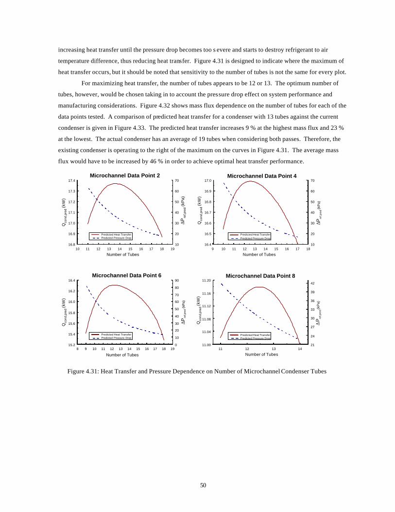
50
increasing heat transfer until the pressure drop becomes too s evere and starts to destroy refrigerant to air
temperature difference, thus reducing heat transfer. Figure 4.31 is designed to indicate where the maximum of
heat transfer occurs, but it should be noted that sensitivity to the number of tubes is not the same for every plot.
For maximizing heat transfer, the number of tubes appears to be 12 or 13. The optimum number of
tubes, however, would be chosen taking in to account the pressure drop effect on system performance and
manufacturing considerations. Figure 4.32 shows mass flux dependence on the number of tubes for each of the
data points tested. A comparison of predicted heat transfer for a condenser with 13 tubes against the current
condenser is given in Figure 4.33. The predicted heat transfer increases 9 % at the highest mass flux and 23 %
at the lowest. The actual condenser has an average of 19 tubes when considering both passes. Therefore, the
existing condenser is operating to the right of the maximum on the curves in Figure 4.31. The average mass
flux would have to be increased by 46 % in order to achieve optimal heat transfer performance.
10 11 12 13 14 15 16 17 18 19
Number of Tubes
16.8
16.9
17.0
17.1
17.2
17.3
17.4
Qco
nd,p
red
(kW
)
10
20
30
40
50
60
70∆P
ref,p
red
(kP
a)
Predicted Heat TransferPredicted Pressure Drop
Microchannel Data Point 2
9 10 11 12 13 14 15 16 17 18
Number of Tubes
16.4
16.5
16.6
16.7
16.8
16.9
17.0
Qco
nd,p
red
(kW
)
10
20
30
40
50
60
70
∆Pre
f,pre
d (k
Pa)
Predicted Heat TransferPredicted Pressure Drop
Microchannel Data Point 4
8 9 10 11 12 13 14 15 16 17 18 19
Number of Tubes
15.2
15.4
15.6
15.8
16.0
16.2
16.4
Qco
nd,p
red
(kW
)
0
10
20
30
40
50
60
70
80
90
∆Pre
f,pre
d (k
Pa)
Predicted Heat TransferPredicted Pressure Drop
Microchannel Data Point 6
11 12 13 14
Number of Tubes
11.00
11.04
11.08
11.12
11.16
11.20
Qco
nd,p
red
(kW
)
21
24
27
30
33
36
39
42
∆P re
f,pre
d (k
Pa)
Predicted Heat TransferPredicted Pressure Drop
Microchannel Data Point 8
Figure 4.31: Heat Transfer and Pressure Dependence on Number of Microchannel Condenser Tubes
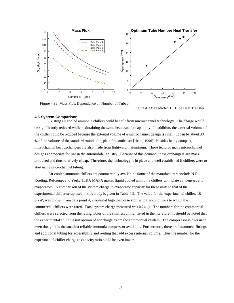
51
8 10 12 14 16 18 20
Number of Tubes
30
40
50
60
70
80
90
100
110
120
Gre
f (kg
/m2 -s
ec)
Mass Flux
Data Point 2Data Point 4Data Point 6Data Point 8
6 8 10 12 14 16 18
Qpred,existing (kW)
6
8
10
12
14
16
18
Qpr
ed,o
ptim
um (k
W)
Optimum Tube Number Heat Transfer
Figure 4.32: Mass Flu x Dependence on Number of Tubes Figure 4.33: Predicted 13 Tube Heat Transfer
4.6 System Comparison Existing air cooled ammonia chillers could benefit from microchannel technology. The charge would
be significantly reduced while maintaining the same heat transfer capability. In addition, the external volume of
the chiller could be reduced because the external volume of a microchannel design is small. It can be about 30
% of the volume of the standard round tube, plate fin condenser [Heun, 1996]. Besides being compact,
microchannel heat exchangers are also made from lightweight aluminum. These features make microchannel
designs appropriate for use in the automobile industry. Because of this demand, these exchangers are mass
produced and thus relatively cheap. Therefore, the technology is in place and well established if chillers were to
start using microchannel tubing.
Air cooled ammonia chillers are commercially available. Some of the manufacturers include N.R.
Koeling, Refcomp, and York. ILKA MAFA makes liquid cooled ammonia chillers with plate condensers and
evaporators. A comparison of the system charge to evaporator capacity for these units to that of the
experimental chiller setup used in this study is given in Table 4.2. The value for the experimental chiller, 18
g/kW, was chosen from data point 4, a nominal high load case similar to the conditions to which the
commercial chillers were rated. Total system charge measured was 0.24 kg. The numbers for the commercial
chillers were selected from the rating tables of the smallest chiller listed in the literature. It should be noted that
the experimental chiller is not optimized for charge as are the commercial chillers. The compressor is oversized
even though it is the smallest reliable ammonia compressor available. Furthermore, there are instrument fittings
and additional tubing for accessibility and routing that add excess internal volume. Thus the number for the
experimental chiller charge to capacity ratio could be even lower.

52
Table 4.2: Ammonia Chiller Charge Comparison
Chiller System Capacity, evap (kW) Charge (g/kW)
Experimental Microchannel Setup 13 18 ILKA MAFA 100.2-11K45 (water cooled) 108 23
Refcomp VKA16-14 16 125 York YSLC F4F00UW 220 129
N.R. Koeling LK 25 25 159
53
Chapter 5: Conclusions and Recommendations
5.1 Summary and Conclusions The objective of this work was to show the benefits of using ammonia with microchannel heat
exchangers. Charge reduction is a constant goal of those who use ammonia in refrigeration and air conditioning
systems. The microchannel tube design that is widely used in the automotive industry could also be used to
reduce the charge of larger ammonia chil lers.
An ammonia chiller test bed and calorimetric wind tunnel were constructed to study condenser
performance. Heat transfer, pressure drop, and charge measurements were taken for two types of condensers:
serpentine flat macro tube and parallel flow microchannel tube. Overall condenser performance was quantified
in terms of heat capacity, refrigerant and air side pressure drops, U values, and refrigerant inventory.
Comparisons between the two similarly sized condensers show the superiority of the microchannel design.
The overall microchannel condenser heat transfer coefficient for a given face velocity is 60-80 %
higher than for the serpentine condenser. Microchannel charge is an average of 53 % less. The charge per
condenser capacity ratios of the microchannel condenser are an average of 76 % less. The microchannel
condenser has a smaller external volume for approximately the same face area.
System charge was measured and compared to other ammonia chillers to show how air cooled
commercial systems could benefit from microchannel technology. The experimental microchannel chiller has
18 g system charge per kW evaporative capacity at similar conditions to the chiller ratings. The other smallest
commercially available air cooled ammonia chillers all have ratios greater than 100 g/kW.
A finite difference model was used to compare the experimental results with existing correlation
predictions. The serpentine condenser had better agreement between the experimentally determined results and
the model predictions because of the absence of headers. Even though the serpentine condenser under
performed experimentally, its simple refrigerant flow configuration allows for a better comparison between
experimental and predicted results. It was found that any of the correlations used in the prediction of ammonia
heat transfer yields an average error around 2 %. Similarly, any of the void fraction correlations applied to
ammonia gives total condenser charge predictions with an average error of 9-12 %.
Temperature distribution data was evaluated to determine the effects of refrigerant mal-distribution
from a microchannel header. Local air exit temperatures were taken with a thermocouple grid. An infrared
camera measurement of tube surface temperatures was performed. Furthermore, a single tube condenser model
was developed using these temperature distribution data to help quantify the heat transfer losses from mal-
distribution. It was found that the average heat transfer loss in the second microchannel pass due to the
introduction of mal-distribution in the model is 11 %.
5.2 Recommendations This work spanned many areas of heat exchanger analysis. A more concentrated study in any of the
areas covered is the next step if further investigation is warranted. For example, the effects of header refrigerant
mal-distribution were only glimpsed and future work should make more extensive research. Some of the tools

54
used in this study could be used to help gain a better understanding of the physics of stratification and flow in
microchannel headers.
The predictions from existing correlations with ammonia should be compared to experimental results
using simple flow geometries such as in a single tube facility. A single tube study would reduce the uncertainty
of external resistance in the prediction of heat transfer. An investigation with a broad range of experimental
parameters could then be conducted to develop microchannel correlations for use with ammonia. In addition,
there is limited to no data for flow inside microchannel ports. Such research would support correlation
development through the creation of a microchannel flow regime map.
There should also be a material compatibility study of aluminum alloys with ammonia. High discharge
temperatures into the condenser could cause some material degradation. Corrosion rates and other quantifiable
data should be taken before designs using high temperature ammonia and aluminum are marketed.
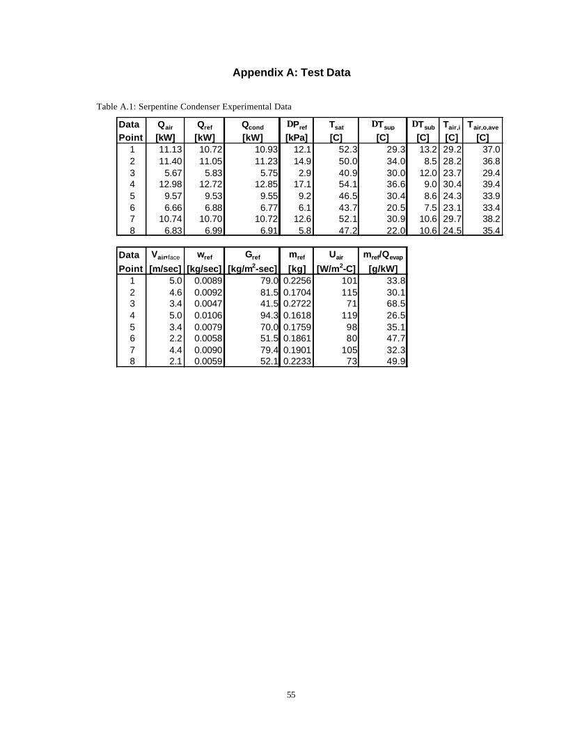
55
Appendix A: Test Data
Table A.1: Serpentine Condenser Experimental Data
Data Qair Qref Qcond ∆Pref Tsat ∆Tsup ∆Tsub Tair,i Tair,o,ave
Point [kW] [kW] [kW] [kPa] [C] [C] [C] [C] [C]1 11.13 10.72 10.93 12.1 52.3 29.3 13.2 29.2 37.02 11.40 11.05 11.23 14.9 50.0 34.0 8.5 28.2 36.83 5.67 5.83 5.75 2.9 40.9 30.0 12.0 23.7 29.44 12.98 12.72 12.85 17.1 54.1 36.6 9.0 30.4 39.45 9.57 9.53 9.55 9.2 46.5 30.4 8.6 24.3 33.96 6.66 6.88 6.77 6.1 43.7 20.5 7.5 23.1 33.47 10.74 10.70 10.72 12.6 52.1 30.9 10.6 29.7 38.28 6.83 6.99 6.91 5.8 47.2 22.0 10.6 24.5 35.4
Data Vair,face wref Gref mref Uair mref/Qevap
Point [m/sec] [kg/sec] [kg/m2-sec] [kg] [W/m2-C] [g/kW]1 5.0 0.0089 79.0 0.2256 101 33.82 4.6 0.0092 81.5 0.1704 115 30.13 3.4 0.0047 41.5 0.2722 71 68.54 5.0 0.0106 94.3 0.1618 119 26.55 3.4 0.0079 70.0 0.1759 98 35.16 2.2 0.0058 51.5 0.1861 80 47.77 4.4 0.0090 79.4 0.1901 105 32.38 2.1 0.0059 52.1 0.2233 73 49.9
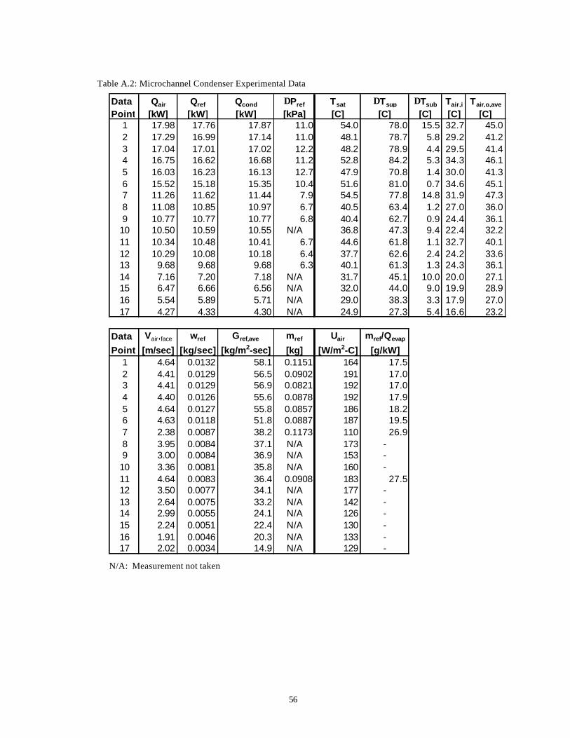
56
Table A.2: Microchannel Condenser Experimental Data
Data Qair Qref Qcond ∆Pref Tsat ∆Tsup ∆Tsub Tair,i Tair,o,ave
Point [kW] [kW] [kW] [kPa] [C] [C] [C] [C] [C]1 17.98 17.76 17.87 11.0 54.0 78.0 15.5 32.7 45.02 17.29 16.99 17.14 11.0 48.1 78.7 5.8 29.2 41.23 17.04 17.01 17.02 12.2 48.2 78.9 4.4 29.5 41.44 16.75 16.62 16.68 11.2 52.8 84.2 5.3 34.3 46.15 16.03 16.23 16.13 12.7 47.9 70.8 1.4 30.0 41.36 15.52 15.18 15.35 10.4 51.6 81.0 0.7 34.6 45.17 11.26 11.62 11.44 7.9 54.5 77.8 14.8 31.9 47.38 11.08 10.85 10.97 6.7 40.5 63.4 1.2 27.0 36.09 10.77 10.77 10.77 6.8 40.4 62.7 0.9 24.4 36.1
10 10.50 10.59 10.55 N/A 36.8 47.3 9.4 22.4 32.211 10.34 10.48 10.41 6.7 44.6 61.8 1.1 32.7 40.112 10.29 10.08 10.18 6.4 37.7 62.6 2.4 24.2 33.613 9.68 9.68 9.68 6.3 40.1 61.3 1.3 24.3 36.114 7.16 7.20 7.18 N/A 31.7 45.1 10.0 20.0 27.115 6.47 6.66 6.56 N/A 32.0 44.0 9.0 19.9 28.916 5.54 5.89 5.71 N/A 29.0 38.3 3.3 17.9 27.017 4.27 4.33 4.30 N/A 24.9 27.3 5.4 16.6 23.2
Data Vair,face wref Gref,ave mref Uair mref/Qevap
Point [m/sec] [kg/sec] [kg/m2-sec] [kg] [W/m2-C] [g/kW]1 4.64 0.0132 58.1 0.1151 164 17.52 4.41 0.0129 56.5 0.0902 191 17.03 4.41 0.0129 56.9 0.0821 192 17.04 4.40 0.0126 55.6 0.0878 192 17.95 4.64 0.0127 55.8 0.0857 186 18.26 4.63 0.0118 51.8 0.0887 187 19.57 2.38 0.0087 38.2 0.1173 110 26.98 3.95 0.0084 37.1 N/A 173 -9 3.00 0.0084 36.9 N/A 153 -
10 3.36 0.0081 35.8 N/A 160 -11 4.64 0.0083 36.4 0.0908 183 27.512 3.50 0.0077 34.1 N/A 177 -13 2.64 0.0075 33.2 N/A 142 -14 2.99 0.0055 24.1 N/A 126 -15 2.24 0.0051 22.4 N/A 130 -16 1.91 0.0046 20.3 N/A 133 -17 2.02 0.0034 14.9 N/A 129 -
N/A: Measurement not taken
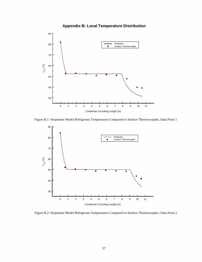
57
Appendix B: Local Temperature Distribution
0 1 2 3 4 5 6 7 8 9 10 11
Condenser Circuiting Length (m)
30
40
50
60
70
80
90
Tre
f (°C
)PredictedSurface Thermocouple
Figure B.1: Serpentine Model Refrigerant Temperatures Compared to Surface Thermocouples, Data Point 1
0 1 2 3 4 5 6 7 8 9 10 11
Condenser Circuiting Length (m)
30
40
50
60
70
80
90
Tre
f (°C
)
PredictedSurface Thermocouple
Figure B.2: Serpentine Model Refrigerant Temperatures Compared to Surface Thermocouples, Data Point 2
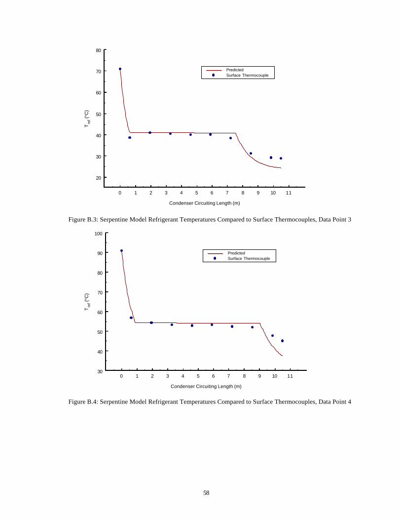
58
0 1 2 3 4 5 6 7 8 9 10 11
Condenser Circuiting Length (m)
20
30
40
50
60
70
80
Tre
f (°C
)
PredictedSurface Thermocouple
Figure B.3: Serpentine Model Refrigerant Temperatures Compared to Surface Thermocouples, Data Point 3
0 1 2 3 4 5 6 7 8 9 10 11
Condenser Circuiting Length (m)
30
40
50
60
70
80
90
100
Tre
f (°C
)
PredictedSurface Thermocouple
Figure B.4: Serpentine Model Refrigerant Temperatures Compared to Surface Thermocouples, Data Point 4
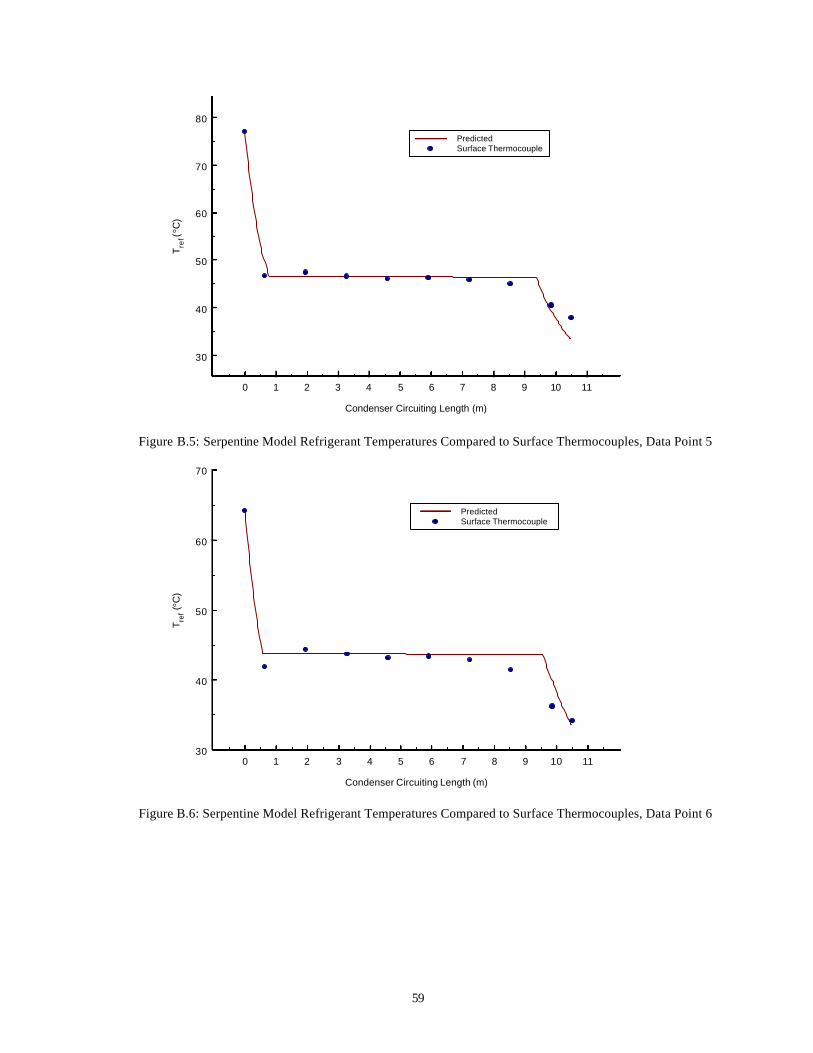
59
0 1 2 3 4 5 6 7 8 9 10 11
Condenser Circuiting Length (m)
30
40
50
60
70
80
Tre
f (°C
)
PredictedSurface Thermocouple
Figure B.5: Serpentine Model Refrigerant Temperatures Compared to Surface Thermocouples, Data Point 5
0 1 2 3 4 5 6 7 8 9 10 11
Condenser Circuiting Length (m)
30
40
50
60
70
Tre
f (°C
)
PredictedSurface Thermocouple
Figure B.6: Serpentine Model Refrigerant Temperatures Compared to Surface Thermocouples, Data Point 6
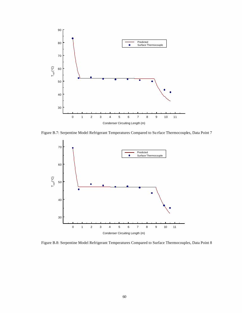
60
0 1 2 3 4 5 6 7 8 9 10 11
Condenser Circuiting Length (m)
30
40
50
60
70
80
90
T re
f (°C
)
PredictedSurface Thermocouple
Figure B.7: Serpentine Model Refrigerant Temperatures Compared to Su rface Thermocouples, Data Point 7
0 1 2 3 4 5 6 7 8 9 10 11
Condenser Circuiting Length (m)
30
40
50
60
70
Tre
f (°C
)
PredictedSurface Thermocouple
Figure B.8: Serpentine Model Refrigerant Temperatures Compared to Surface Thermocouples, Data Point 8
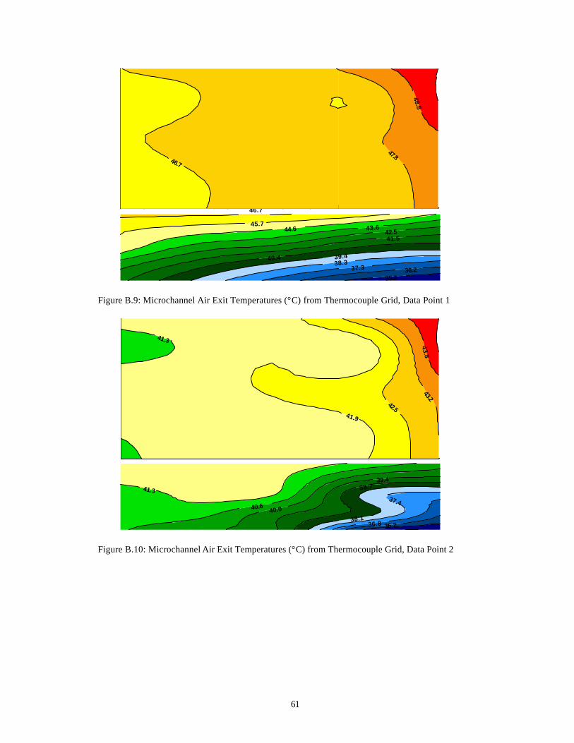
61
35.2 36.2 37.3
38.3 39.4 40.4
41.5 42.5 43.6 44.6
45.7
46.7
46.7
47.8 48.8
Figure B.9: Microchannel Air Exit Temperatures (°C) from Thermocouple Grid, Data Point 1
36.2 36.8
37.4
38.1
38.7 39.4
40.0 40.6
41.3
41.3
41.9
42.5
43.2 43.8
Figure B.10: Microchannel Air Exit Temperatures (°C) from Thermocouple Grid, Data Point 2
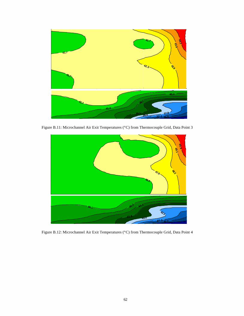
62
36.5 37.1 37.8
38.4 39.1
39.7
40.4
41.0
41.7
41.7
41.7
41.7
42.3
42.9 43.6
44.2
Figure B.11: Microchannel Air Exit Temperatures (°C) from Thermocouple Grid, Data Point 3
40.7 41.5
42.3
43.0 43.8
44.5 45.3 46.1
46.8
47.6
48.3 49.1
49.8
Figure B.12: Microchannel Air Exit Temperatures (°C) from Thermocouple Grid, Data Point 4

63
36.0 37.3 38.0 38.6
39.3
39.9 40.6
41.2
41.9
41.9
41.9
42.5
43.2 43.8
Figure B.13: Microchannel Air Exit Temperatures (°C) from Thermocouple Grid, Data Point 5
38.5 39.3
40.1
40.9 41.8 42.6
43.4
44.2
45.0 45.8
45.8
45.8
46.6
47.5
48.3
Figure B.14: Microchannel Air Exit Temperatures (°C) from Thermocouple Grid, Data Point 6
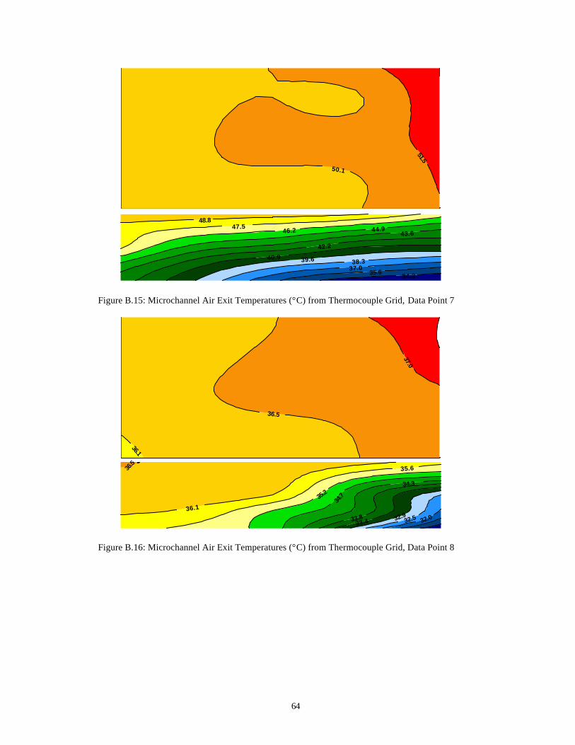
64
34.3 35.6 37.0 38.3 39.6 40.9
42.2
43.6 44.9 46.2 47.5 48.8
50.1
51.5
Figure B.15: Microchannel Air Exit Temperatures (°C) from Thermocouple Grid, Data Point 7
32.0 32.5 32.9 33.4 33.8
34.3
34.7 35
.2
35.6
36.1
36.5
36.1
36.5
37.0
Figure B.16: Microchannel Air Exit Temperatures (°C) from Thermocouple Grid, Data Point 8
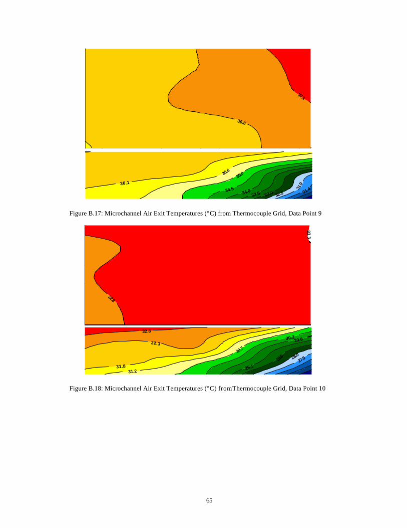
65
31.4 31.9
32.5 33.0 33.5 34.0 34.5
35.0 35.6
36.1
36.6
37.1
Figure B.17: Microchannel Air Exit Temperatures (°C) from Thermocouple Grid, Data Point 9
27.5 28
.0 28
.6
29.1
29.6 30.2
30.7
31.2 31.8
32.3
32.8
32.8
33.3
Figure B.18: Microchannel Air Exit Temperatures (°C) from Thermocouple Grid, Data Point 10
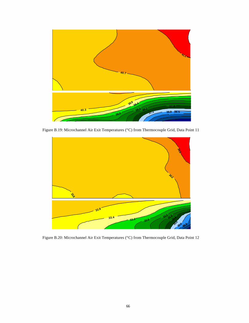
66
36.5 36.9 37.3
37.8 38.2 38.6
39.0
39.4 39.9
40.3
40.7
41.1
Figure B.19: Microchannel Air Exit Temperatures (°C) from Thermocouple Grid, Data Point 11
30.2 30.6 31
.0 31
.4 31.8 32.2
32.6 33.0 33.4
33.8
33.8 34.2
34.6
Figure B.20: Microchannel Air Exit Temperatures (°C) from Thermocouple Grid, Data Point 12
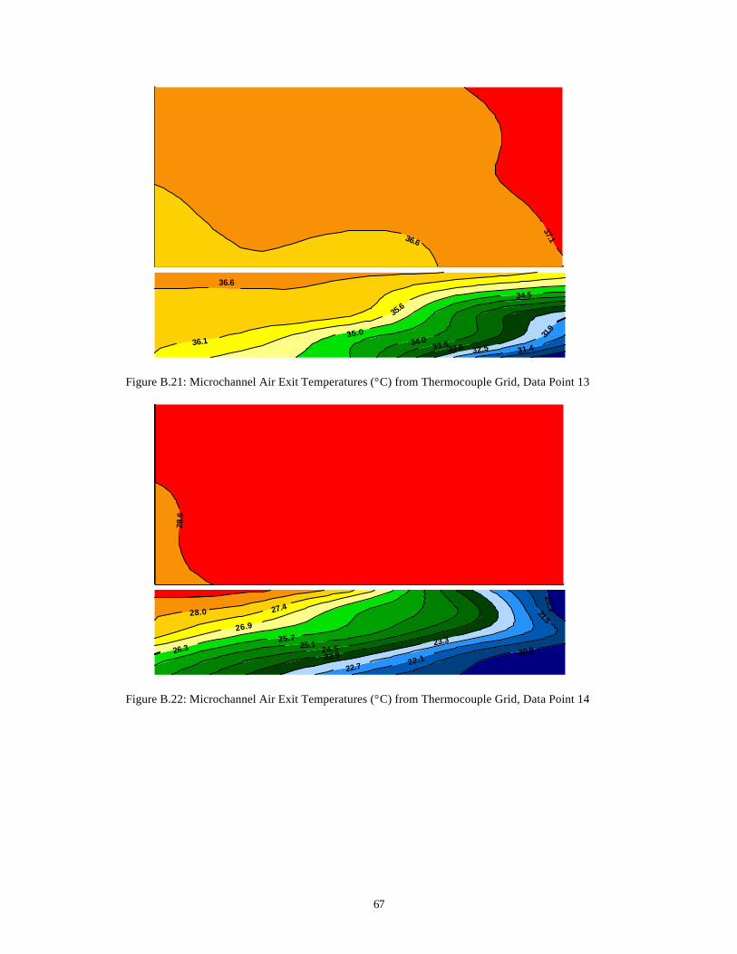
67
31.4
31.9
32.5 33.0 33.5 34.0
34.5
35.0
35.6
36.1
36.6
36.6
37.1
Figure B.21: Microchannel Air Exit Temperatures (°C) from Thermocouple Grid, Data Point 13
20.9
20.9
21.5
22.1 22.7
23.3
23.9 24.5 25.1
25.7
26.3
26.9
27.4 28.0
28.
6
Figure B.22: Microchannel Air Exit Temperatures (°C) from Thermocouple Grid, Data Point 14
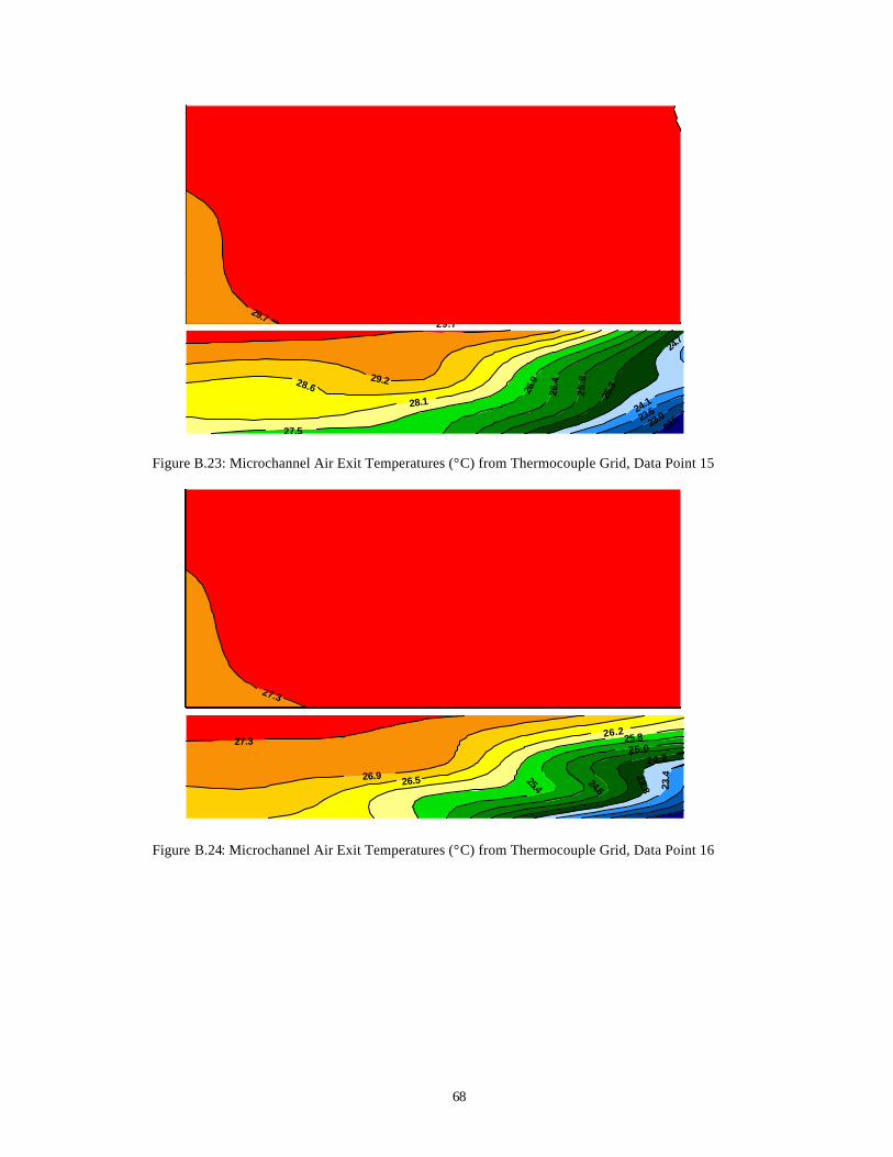
68
22.5 23.0 23
.6 24.1
24.7
25.
3
25.
8
26.
4
26.
9
27.5
28.1
28.6 29.2
29.7 29.7
Figure B.23: Microchannel Air Exit Temperatures (°C) from Thermocouple Grid, Data Point 15
23.
4 23.8
24.2
24.6
25.0
25.4
25.8 26.2
26.5 26.9
27.3
27.3
Figure B.24: Microchannel Air Exit Temperatures (°C) from Thermocouple Grid, Data Point 16
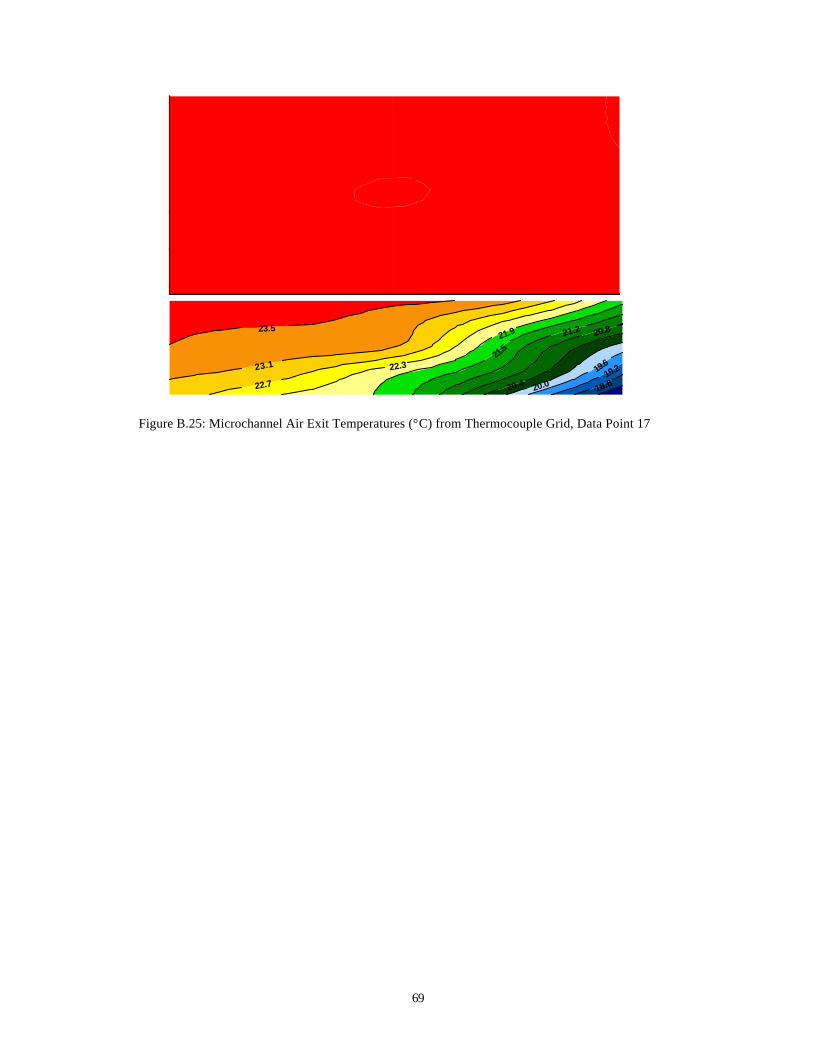
69
18.8 19.2 19.6
20.0 20.4
20.8 21.2
21.5
21.9
22.3
22.7
23.1
23.5
Figure B.25: Microchannel Air Exit Temperatures (°C) from Thermocouple Grid, Data Point 17
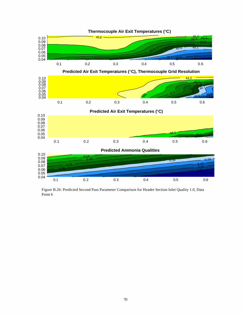
70
0.1 0.2 0.3 0.4 0.5 0.60.040.050.060.070.080.090.10
38.5 39.3
40.1 40.9
41.8
42.6
43.4 44.2 45.0 45.8
Thermocouple Air Exit Temperatures (°C)
0.1 0.2 0.3 0.4 0.5 0.60.040.050.060.070.080.090.10
39.5 40.1
40.7 41.2
41.8
42.4
43.0
43.6
44.2
Predicted Air Exit Temperatures (°C), Thermocouple Grid Resolution
0.1 0.2 0.3 0.4 0.5 0.60.040.050.060.070.080.090.10
43.2 44.1
Predicted Air Exit Temperatures (°C)
0.1 0.2 0.3 0.4 0.5 0.60.040.050.060.070.080.090.10
0.06 0.12 0.18
0.24 0.30
0.36 0.42
0.48 0.54
Predicted Ammonia Qualities
Figure B.26: Predicted Second Pass Parameter Comparison for Header Section Inlet Quality 1.0, Data Point 6
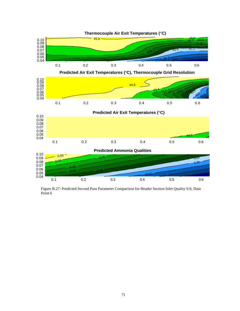
71
0.1 0.2 0.3 0.4 0.5 0.60.040.050.060.070.080.090.10
38.5 39.3
40.1 40.9
41.8
42.6
43.4 44.2 45.0 45.8
Thermocouple Air Exit Temperatures (°C)
0.1 0.2 0.3 0.4 0.5 0.60.040.050.060.070.080.090.10
43.0 43.2 43
.4 43.6 43.8 44.0 44.2 44.4 44.6
Predicted Air Exit Temperatures (°C), Thermocouple Grid Resolution
0.1 0.2 0.3 0.4 0.5 0.60.040.050.060.070.080.090.10
44.1
Predicted Air Exit Temperatures (°C)
Predicted Ammonia Qualities
0.1 0.2 0.3 0.4 0.5 0.60.040.050.060.070.080.090.10
0.10 0.15
0.20 0.25
0.30 0.35 0.40
0.45 0.50
0.55
Figure B.27: Predicted Second Pass Parameter Comparison for Header Section Inlet Quality 0.8, Data Point 6
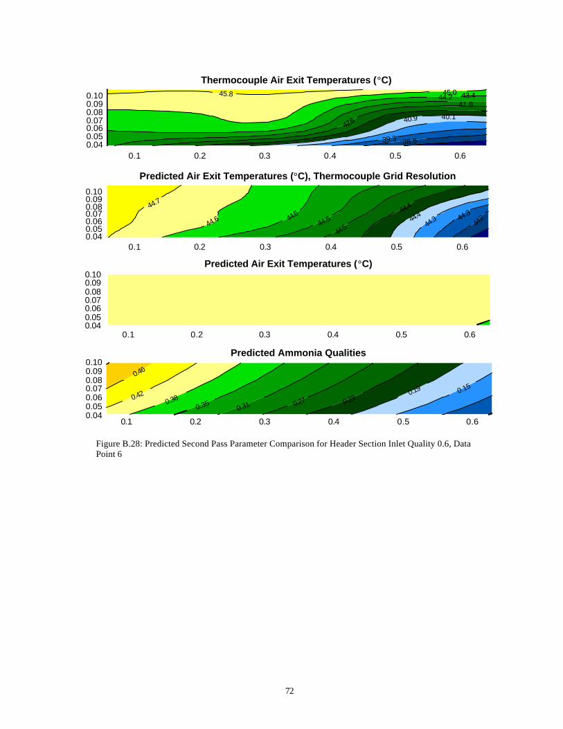
72
0.1 0.2 0.3 0.4 0.5 0.60.040.050.060.070.080.090.10
38.5 39.3
40.1 40.9
41.8
42.6
43.4 44.2 45.0 45.8
Thermocouple Air Exit Temperatures (°C)
0.1 0.2 0.3 0.4 0.5 0.60.040.050.060.070.080.090.10
44.2 44.3
44.3 44
.4 44
.4
44.5 44.5 44
.6
44.6
44.7
Predicted Air Exit Temperatures (°C), Thermocouple Grid Resolution
0.1 0.2 0.3 0.4 0.5 0.60.040.050.060.070.080.090.10
Predicted Air Exit Temperatures (°C)
0.1 0.2 0.3 0.4 0.5 0.60.040.050.060.070.080.090.10
0.15 0.19
0.23 0.27
0.31 0.35 0.38 0.42
0.46
Predicted Ammonia Qualities
Figure B.28: Predicted Second Pass Parameter Comparison for Header Section Inlet Quality 0.6, Data Point 6
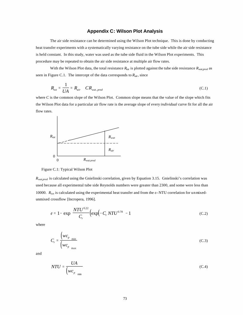
73
Appendix C: Wilson Plot Analysis
The air side resistance can be determined using the Wilson Plot technique. This is done by conducting
heat transfer experiments with a systematically varying resistance on the tube side while the air side resistance
is held constant. In this study, water was used as the tube side fluid in the Wilson Plot experiments. This
procedure may be repeated to obtain the air side resistance at multiple air flow rates.
With the Wilson Plot data, the total resistance Rtot is plotted against the tube side resistance Rwat,pred as
seen in Figure C.1. The intercept of the data corresponds to Rair, since
RUA
R CRtot air wat pred= = +1
, (C.1)
where C is the common slope of the Wilson Plot. Common slope means that the value of the slope which fits
the Wilson Plot data for a particular air flow rate is the average slope of every individual curve fit for all the air
flow rates.
Figure C.1: Typical Wilson Plot
Rwat,pred is calculated using the Gnielinski correlation, given by Equation 3.15. Gnielinski’s correlation was
used because all experimental tube side Reynolds numbers were greater than 2300, and some were less than
10000. Rtot is calculated using the experimental heat transfer and from the ε–NTU correlation for unmixed-
unmixed crossflow [Incropera, 1996].
( )( )ε = − − −
1 1
0 220 78exp exp
..NTU
CC NTU
rr (C.2)
where
( )( )Cwc
wcr
p
p
= min
max
(C.3)
and
( )NTUUA
wcp
=min
(C.4)
Rwat
Rair
Rtot
Rwat,pred 0 0
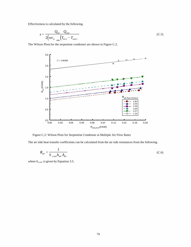
74
Effectiveness is calculated by the following.
( ) ( )ε =+
−
Q Q
wc T Tair wat
p air i wat i2min , ,
(C.5)
The Wilson Plots for the serpentine condenser are shown in Figure C.2.
0.00 0.02 0.04 0.06 0.08 0.10 0.12 0.14 0.16 0.18
Rwat,pred (K/kW)
0.0
0.5
1.0
1.5
2.0
2.5
3.0
Rto
t (K
/kW
)
C = 2.80383
4.804.093.382.692.071.26
Vair,face (m/sec)
Figure C.2: Wilson Plots for Serpentine Condenser at Multiple Air Flow Rates
The air side heat transfer coefficients can be calculated from the air side resistances from the following.
Rh Aair
o air air air
=1
η ,
(C.6)
where ηo,air is given by Equation 3.5.

75
Appendix D: Simulation Code
This appendix contains the simulation code for the microchannel condenser single tube model. Also
included are calculations of experimental parameters such as measured charge, heat transfer, and air mass flow
rate. Variable model inputs are read into the EES code via the LOOKUP() function. Line continuation is
denoted with the ampersand, &. Comments are enclosed in braces, {}
{Calculate Reynolds number from mass flux, diameter, and dynamic &viscosity} PROCEDURE ReyN(G,D,mu:Re) Re = G*D/mu END {Calculate experimental condenser heat transfer} FUNCTION Q_cond_exp(m_dot,T_i,P_i,T_o,P_o) Qi =m_dot*(ENTHALPY(Ammonia,T=T_i,P=P_i) &+.0005*(4*m_dot*VOLUME(Ammonia,T=T_i,P=P_i)/PI/(.4*.0254)^2)^2) Qo=m_dot*(ENTHALPY(Ammonia,P=P_o,T=T_o) &+.0005*(4*m_dot*VOLUME(Ammonia,T=T_o,P=P_o)/PI/(.3*.0254)^2)^2) Q_cond_exp := Qi-Qo END {Calculate effective compressor work} FUNCTION Comp_work(m_dot,T_i,P_i,T_o,P_o) h_i = ENTHALPY(Ammonia,T=T_i,P=P_i) h_o = ENTHALPY(Ammonia,T=T_o,P=P_o) Comp_work = m_dot*(h_o-h_i) END {Calculate subcooling and superheating of refrigerant} PROCEDURE Sub_Sup(P_i,P_o,T_i,T_o:T_sat,DELTAT_sub,DELTAT_sup) T_sat = TEMPERATURE(Ammonia,P=(P_i+P_o)/2,X=0.5) T_sat_sub = TEMPERATURE(Ammonia,P=P_o,X=0.5) T_sat_sup = TEMPERATURE(Ammonia,P=P_i,X=0.5) DELTAT_sup = T_i-T_sat_sup DELTAT_sub = T_sat_sub-T_o END {Calculate experimental charge of condenser} PROCEDURE Charge_exp(P1,T1,P2,T2,P3,T3,Vol_xtra1,Vol_xtra2,Volume_cnd, &M_cyl,P_o,T_o,m_xtra1:m,m_xtra2,m_left) {total volume of space occupied between shut-off valves} Volume = Vol_xtra1+Vol_xtra2+Volume_cnd T_sat1 = TEMPERATURE(Ammonia,P=P1,X=0.5) T_sat2 = TEMPERATURE(Ammonia,P=P2,X=0.5) T_sat3 = TEMPERATURE(Ammonia,P=P3,X=0.5) v_o = VOLUME(Ammonia,T=T_o,P=P_o) IF (T_sat1=T1) OR (T_sat2=T2) OR (T_sat3=T3) THEN CALL ERROR('T_sat_after = T_after') ELSE m1 = 1/VOLUME(Ammonia,T=T1,P=P1)*Volume m2 = 1/VOLUME(Ammonia,T=T2,P=P2)*Volume m3 = 1/VOLUME(Ammonia,T=T3,P=P3)*Volume ENDIF
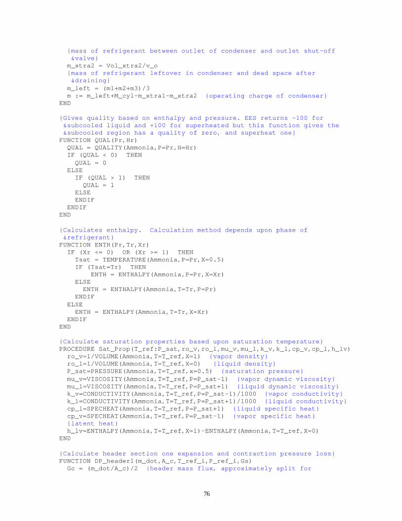
76
{mass of refrigerant between outlet of condenser and outlet shut-off &valve} m_xtra2 = Vol_xtra2/v_o {mass of refrigerant leftover in condenser and dead space after &draining} m_left = (m1+m2+m3)/3 m := m_left+M_cyl-m_xtra1-m_xtra2 {operating charge of condenser} END {Gives quality based on enthalpy and pressure. EES returns -100 for &subcooled liquid and +100 for superheated but this function gives the &subcooled region has a quality of zero, and superheat one} FUNCTION QUAL(Pr,Hr) QUAL = QUALITY(Ammonia,P=Pr,H=Hr) IF (QUAL < 0) THEN QUAL = 0 ELSE IF (QUAL > 1) THEN QUAL = 1 ELSE ENDIF ENDIF END {Calculates enthalpy. Calculation method depends upon phase of &refrigerant} FUNCTION ENTH(Pr,Tr,Xr) IF (Xr <= 0) OR (Xr >= 1) THEN Tsat = TEMPERATURE(Ammonia,P=Pr,X=0.5) IF (Tsat=Tr) THEN ENTH = ENTHALPY(Ammonia,P=Pr,X=Xr) ELSE ENTH = ENTHALPY(Ammonia,T=Tr,P=Pr) ENDIF ELSE ENTH = ENTHALPY(Ammonia,T=Tr,X=Xr) ENDIF END {Calculate saturation properties based upon saturation temperature} PROCEDURE Sat_Prop(T_ref:P_sat,ro_v,ro_l,mu_v,mu_l,k_v,k_l,cp_v,cp_l,h_lv) ro_v=1/VOLUME(Ammonia,T=T_ref,X=1) {vapor density} ro_l=1/VOLUME(Ammonia,T=T_ref,X=0) {liquid density} P_sat=PRESSURE(Ammonia,T=T_ref,x=0.5) {saturation pressure} mu_v=VISCOSITY(Ammonia,T=T_ref,P=P_sat-1) {vapor dynamic viscosity} mu_l=VISCOSITY(Ammonia,T=T_ref,P=P_sat+1) {liquid dynamic viscosity} k_v=CONDUCTIVITY(Ammonia,T=T_ref,P=P_sat-1)/1000 {vapor conductivity} k_l=CONDUCTIVITY(Ammonia,T=T_ref,P=P_sat+1)/1000 {liquid conductivity} cp_l=SPECHEAT(Ammonia,T=T_ref,P=P_sat+1) {liquid specific heat} cp_v=SPECHEAT(Ammonia,T=T_ref,P=P_sat-1) {vapor specific heat} {latent heat} h_lv=ENTHALPY(Ammonia,T=T_ref,X=1)-ENTHALPY(Ammonia,T=T_ref,X=0) END {Calculate header section one expansion and contraction pressure loss} FUNCTION DP_header1(m_dot,A_c,T_ref_i,P_ref_i,Gs) Gc = (m_dot/A_c)/2 {header mass flux, approximately split for
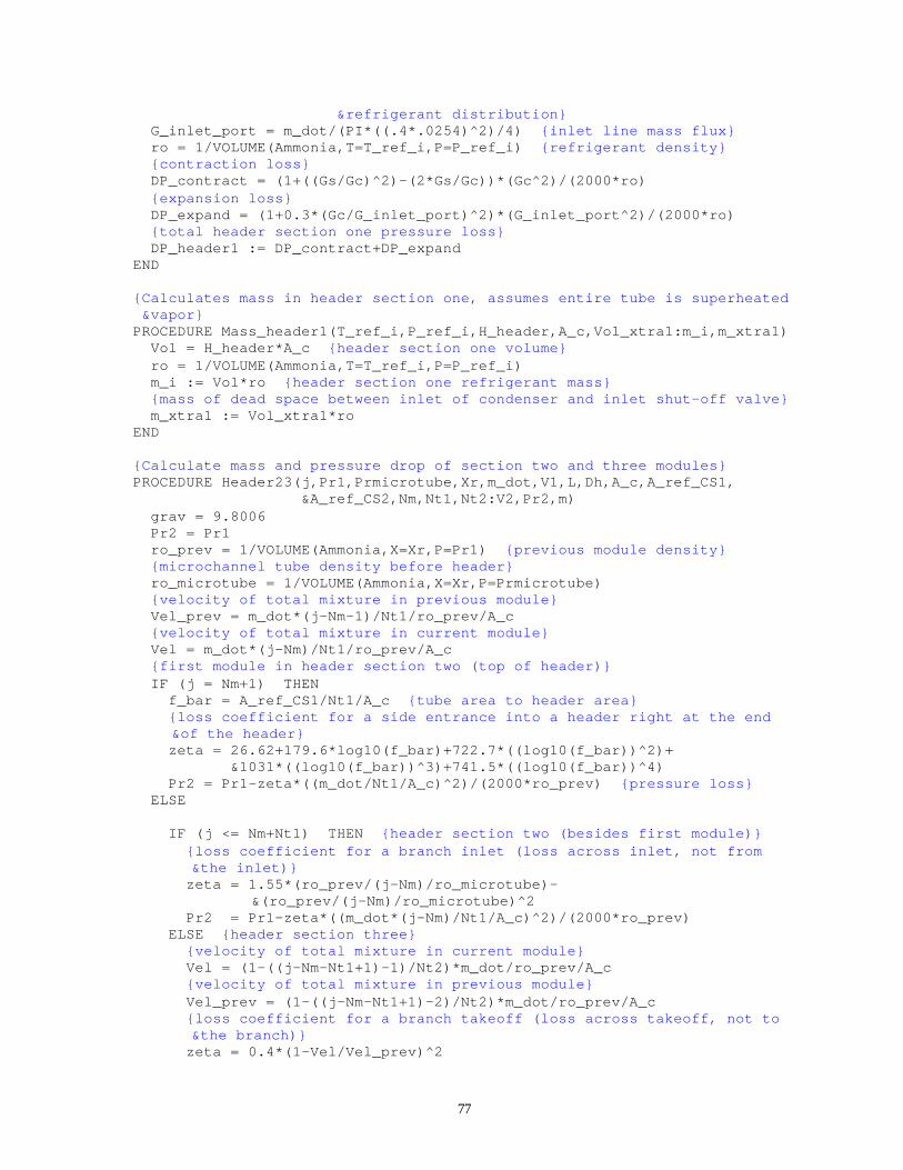
77
&refrigerant distribution} G_inlet_port = m_dot/(PI*((.4*.0254)^2)/4) {inlet line mass flux} ro = 1/VOLUME(Ammonia,T=T_ref_i,P=P_ref_i) {refrigerant density} {contraction loss} DP_contract = (1+((Gs/Gc)^2)-(2*Gs/Gc))*(Gc^2)/(2000*ro) {expansion loss} DP_expand = (1+0.3*(Gc/G_inlet_port)^2)*(G_inlet_port^2)/(2000*ro) {total header section one pressure loss} DP_header1 := DP_contract+DP_expand END {Calculates mass in header section one, assumes entire tube is superheated &vapor} PROCEDURE Mass_header1(T_ref_i,P_ref_i,H_header,A_c,Vol_xtra1:m_i,m_xtra1) Vol = H_header*A_c {header section one volume} ro = 1/VOLUME(Ammonia,T=T_ref_i,P=P_ref_i) m_i := Vol*ro {header section one refrigerant mass} {mass of dead space between inlet of condenser and inlet shut-off valve} m_xtra1 := Vol_xtra1*ro END {Calculate mass and pressure drop of section two and three modules} PROCEDURE Header23(j,Pr1,Prmicrotube,Xr,m_dot,V1,L,Dh,A_c,A_ref_CS1, &A_ref_CS2,Nm,Nt1,Nt2:V2,Pr2,m) grav = 9.8006 Pr2 = Pr1 ro_prev = 1/VOLUME(Ammonia,X=Xr,P=Pr1) {previous module density} {microchannel tube density before header} ro_microtube = 1/VOLUME(Ammonia,X=Xr,P=Prmicrotube) {velocity of total mixture in previous module} Vel_prev = m_dot*(j-Nm-1)/Nt1/ro_prev/A_c {velocity of total mixture in current module} Vel = m_dot*(j-Nm)/Nt1/ro_prev/A_c {first module in header section two (top of header)} IF (j = Nm+1) THEN f_bar = A_ref_CS1/Nt1/A_c {tube area to header area} {loss coefficient for a side entrance into a header right at the end &of the header} zeta = 26.62+179.6*log10(f_bar)+722.7*((log10(f_bar))^2)+ &1031*((log10(f_bar))^3)+741.5*((log10(f_bar))^4) Pr2 = Pr1-zeta*((m_dot/Nt1/A_c)^2)/(2000*ro_prev) {pressure loss} ELSE IF (j <= Nm+Nt1) THEN {header section two (besides first module)} {loss coefficient for a branch inlet (loss across inlet, not from &the inlet)} zeta = 1.55*(ro_prev/(j-Nm)/ro_microtube)- &(ro_prev/(j-Nm)/ro_microtube)^2 Pr2 = Pr1-zeta*((m_dot*(j-Nm)/Nt1/A_c)^2)/(2000*ro_prev) ELSE {header section three} {velocity of total mixture in current module} Vel = (1-((j-Nm-Nt1+1)-1)/Nt2)*m_dot/ro_prev/A_c {velocity of total mixture in previous module} Vel_prev = (1-((j-Nm-Nt1+1)-2)/Nt2)*m_dot/ro_prev/A_c {loss coefficient for a branch takeoff (loss across takeoff, not to &the branch)} zeta = 0.4*(1-Vel/Vel_prev)^2
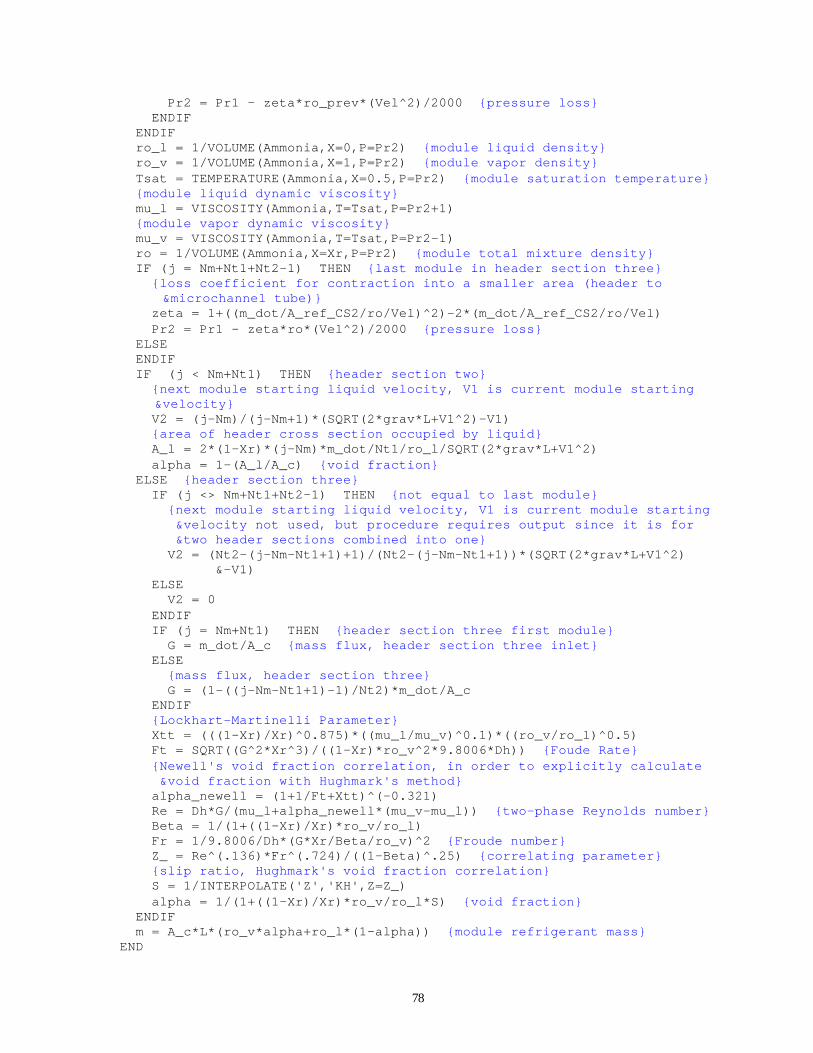
78
Pr2 = Pr1 - zeta*ro_prev*(Vel^2)/2000 {pressure loss} ENDIF ENDIF ro_l = 1/VOLUME(Ammonia,X=0,P=Pr2) {module liquid density} ro_v = 1/VOLUME(Ammonia,X=1,P=Pr2) {module vapor density} Tsat = TEMPERATURE(Ammonia,X=0.5,P=Pr2) {module saturation temperature} {module liquid dynamic viscosity} mu_l = VISCOSITY(Ammonia,T=Tsat,P=Pr2+1) {module vapor dynamic viscosity} mu_v = VISCOSITY(Ammonia,T=Tsat,P=Pr2-1) ro = 1/VOLUME(Ammonia,X=Xr,P=Pr2) {module total mixture density} IF (j = Nm+Nt1+Nt2-1) THEN {last module in header section three} {loss coefficient for contraction into a smaller area (header to µchannel tube)} zeta = 1+((m_dot/A_ref_CS2/ro/Vel)^2)-2*(m_dot/A_ref_CS2/ro/Vel) Pr2 = Pr1 - zeta*ro*(Vel^2)/2000 {pressure loss} ELSE ENDIF IF (j < Nm+Nt1) THEN {header section two} {next module starting liquid velocity, V1 is current module starting &velocity} V2 = (j-Nm)/(j-Nm+1)*(SQRT(2*grav*L+V1^2)-V1) {area of header cross section occupied by liquid} A_l = 2*(1-Xr)*(j-Nm)*m_dot/Nt1/ro_l/SQRT(2*grav*L+V1^2) alpha = 1-(A_l/A_c) {void fraction} ELSE {header section three} IF (j <> Nm+Nt1+Nt2-1) THEN {not equal to last module} {next module starting liquid velocity, V1 is current module starting &velocity not used, but procedure requires output since it is for &two header sections combined into one} V2 = (Nt2-(j-Nm-Nt1+1)+1)/(Nt2-(j-Nm-Nt1+1))*(SQRT(2*grav*L+V1^2) &-V1) ELSE V2 = 0 ENDIF IF (j = Nm+Nt1) THEN {header section three first module} G = m_dot/A_c {mass flux, header section three inlet} ELSE {mass flux, header section three} G = (1-((j-Nm-Nt1+1)-1)/Nt2)*m_dot/A_c ENDIF {Lockhart-Martinelli Parameter} Xtt = (((1-Xr)/Xr)^0.875)*((mu_l/mu_v)^0.1)*((ro_v/ro_l)^0.5) Ft = SQRT((G^2*Xr^3)/((1-Xr)*ro_v^2*9.8006*Dh)) {Foude Rate} {Newell's void fraction correlation, in order to explicitly calculate &void fraction with Hughmark's method} alpha_newell = (1+1/Ft+Xtt)^(-0.321) Re = Dh*G/(mu_l+alpha_newell*(mu_v-mu_l)) {two-phase Reynolds number} Beta = 1/(1+((1-Xr)/Xr)*ro_v/ro_l) Fr = 1/9.8006/Dh*(G*Xr/Beta/ro_v)^2 {Froude number} Z_ = Re^(.136)*Fr^(.724)/((1-Beta)^.25) {correlating parameter} {slip ratio, Hughmark's void fraction correlation} S = 1/INTERPOLATE('Z','KH',Z=Z_) alpha = 1/(1+((1-Xr)/Xr)*ro_v/ro_l*S) {void fraction} ENDIF m = A_c*L*(ro_v*alpha+ro_l*(1-alpha)) {module refrigerant mass} END
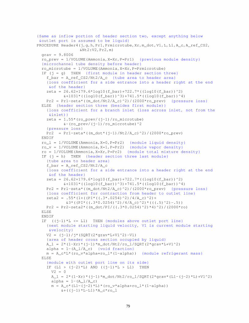
79
{Same as inflow portion of header section two, except anything below &outlet port is assumed to be liquid} PROCEDURE Header4(j,g,h,Pr1,Prmicrotube,Xr,m_dot,V1,L,L1,A_c,A_ref_CS2, &Nt2:V2,Pr2,m) grav = 9.8006 ro_prev = 1/VOLUME(Ammonia,X=Xr,P=Pr1) {previous module density} {microchannel tube density before header} ro_microtube = 1/VOLUME(Ammonia,X=Xr,P=Prmicrotube) IF (j = g) THEN {first module in header section three} f_bar = A_ref_CS2/Nt2/A_c {tube area to header area} {loss coefficient for a side entrance into a header right at the end &of the header} zeta = 26.62+179.6*log10(f_bar)+722.7*((log10(f_bar))^2) &+1031*((log10(f_bar))^3)+741.5*((log10(f_bar))^4) Pr2 = Pr1-zeta*((m_dot/Nt2/A_c)^2)/(2000*ro_prev) {pressure loss} ELSE {header section three (besides first module)} {loss coefficient for a branch inlet (loss across inlet, not from the &inlet)} zeta = 1.55*(ro_prev/(j-1)/ro_microtube) &-(ro_prev/(j-1)/ro_microtube)^2 {pressure loss} Pr2 = Pr1-zeta*((m_dot*(j-1)/Nt2/A_c)^2)/(2000*ro_prev) ENDIF ro_l = 1/VOLUME(Ammonia,X=0,P=Pr2) {module liquid density} ro_v = 1/VOLUME(Ammonia,X=1,P=Pr2) {module vapor density} ro = 1/VOLUME(Ammonia,X=Xr,P=Pr2) {module total mixture density} IF (j = h) THEN {header section three last module} {tube area to header area} f_bar = A_ref_CS2/Nt2/A_c {loss coefficient for a side entrance into a header right at the end &of the header} zeta = 26.62+179.6*log10(f_bar)+722.7*((log10(f_bar))^2) &+1031*((log10(f_bar))^3)+741.5*((log10(f_bar))^4) Pr2 = Pr1-zeta*((m_dot/Nt2/A_c)^2)/(2000*ro_prev) {pressure loss} {loss coefficient for contraction from header to outlet line} zeta2 = .55*(1+((PI*((.3*.0254)^2)/4/A_c)^2)+ &3*((PI*((.3*0.0254)^2)/4/A_c)^2)*(((.5)^2)-.5)) Pr2 = Pr2-zeta2*((m_dot/PI/((.3*0.0254)^2)*4)^2)/(2000*ro) ELSE ENDIF IF ((j-1)*L <= L1) THEN {modules above outlet port line} {next module starting liquid velocity, V1 is current module starting &velocity} V2 = (j-1)/j*(SQRT(2*grav*L+V1^2)-V1) {area of header cross section occupied by liquid} A_l = 2*(1-Xr)*(j-1)*m_dot/Nt2/ro_l/SQRT(2*grav*L+V1^2) alpha = 1-(A_l/A_c) {void fraction} m = A_c*L*(ro_v*alpha+ro_l*(1-alpha)) {module refrigerant mass} ELSE {module with outlet port line on its side} IF (L1 > (j-2)*L) AND ((j-1)*L > L1) THEN V2 = 0 A_l = 2*(1-Xr)*(j-1)*m_dot/Nt2/ro_l/SQRT(2*grav*(L1-(j-2)*L)+V1^2) alpha = 1-(A_l/A_c) m = A_c*(L1-(j-2)*L)*(ro_v*alpha+ro_l*(1-alpha)) &+((j-1)*L-L1)*A_c*ro_l
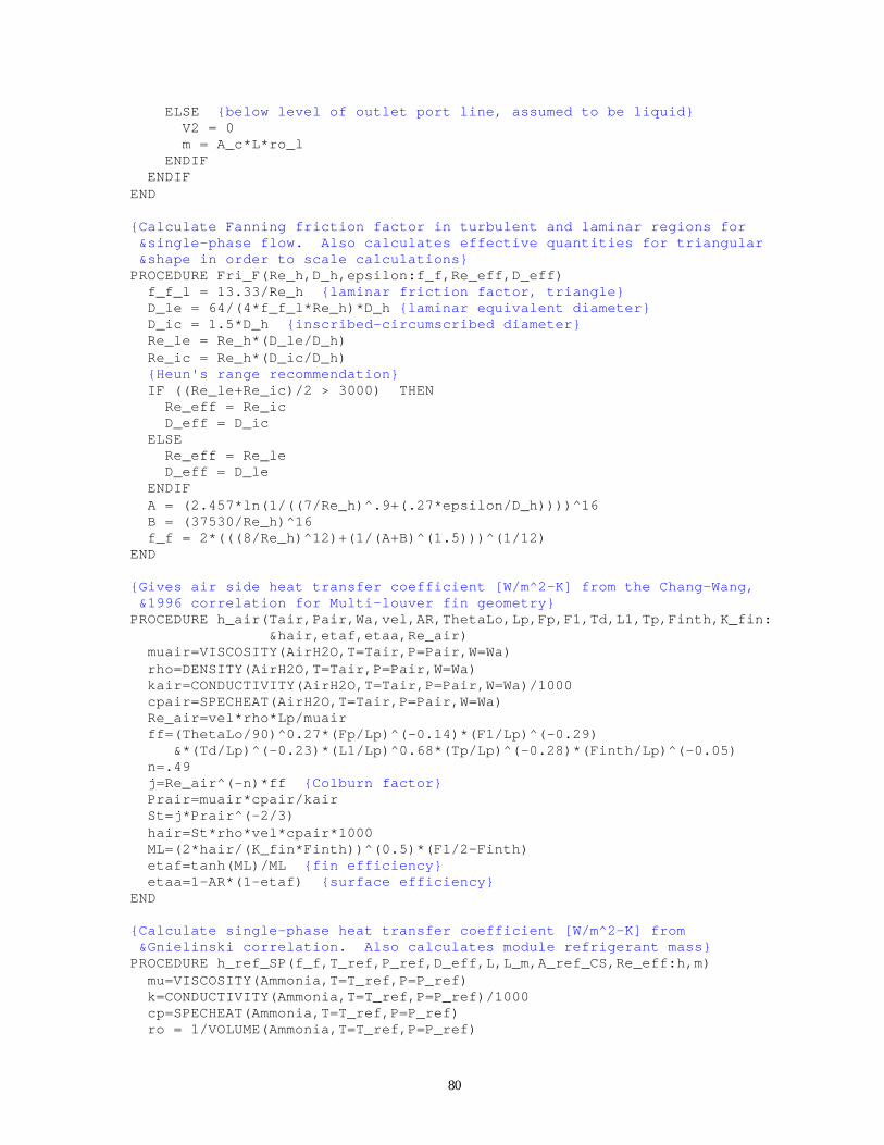
80
ELSE {below level of outlet port line, assumed to be liquid} V2 = 0 m = A_c*L*ro_l ENDIF ENDIF END {Calculate Fanning friction factor in turbulent and laminar regions for &single-phase flow. Also calculates effective quantities for triangular &shape in order to scale calculations} PROCEDURE Fri_F(Re_h,D_h,epsilon:f_f,Re_eff,D_eff) f_f_l = 13.33/Re_h {laminar friction factor, triangle} D_le = 64/(4*f_f_l*Re_h)*D_h {laminar equivalent diameter} D_ic = 1.5*D_h {inscribed-circumscribed diameter} Re_le = Re_h*(D_le/D_h) Re_ic = Re_h*(D_ic/D_h) {Heun's range recommendation} IF ((Re_le+Re_ic)/2 > 3000) THEN Re_eff = Re_ic D_eff = D_ic ELSE Re_eff = Re_le D_eff = D_le ENDIF A = (2.457*ln(1/((7/Re_h)^.9+(.27*epsilon/D_h))))^16 B = (37530/Re_h)^16 f_f = 2*(((8/Re_h)^12)+(1/(A+B)^(1.5)))^(1/12) END {Gives air side heat transfer coefficient [W/m^2-K] from the Chang-Wang, &1996 correlation for Multi-louver fin geometry} PROCEDURE h_air(Tair,Pair,Wa,vel,AR,ThetaLo,Lp,Fp,F1,Td,L1,Tp,Finth,K_fin: &hair,etaf,etaa,Re_air) muair=VISCOSITY(AirH2O,T=Tair,P=Pair,W=Wa) rho=DENSITY(AirH2O,T=Tair,P=Pair,W=Wa) kair=CONDUCTIVITY(AirH2O,T=Tair,P=Pair,W=Wa)/1000 cpair=SPECHEAT(AirH2O,T=Tair,P=Pair,W=Wa) Re_air=vel*rho*Lp/muair ff=(ThetaLo/90)^0.27*(Fp/Lp)^(-0.14)*(F1/Lp)^(-0.29) &*(Td/Lp)^(-0.23)*(L1/Lp)^0.68*(Tp/Lp)^(-0.28)*(Finth/Lp)^(-0.05) n=.49 j=Re_air^(-n)*ff {Colburn factor} Prair=muair*cpair/kair St=j*Prair^(-2/3) hair=St*rho*vel*cpair*1000 ML=(2*hair/(K_fin*Finth))^(0.5)*(F1/2-Finth) etaf=tanh(ML)/ML {fin efficiency} etaa=1-AR*(1-etaf) {surface efficiency} END {Calculate single-phase heat transfer coefficient [W/m^2-K] from &Gnielinski correlation. Also calculates module refrigerant mass} PROCEDURE h_ref_SP(f_f,T_ref,P_ref,D_eff,L,L_m,A_ref_CS,Re_eff:h,m) mu=VISCOSITY(Ammonia,T=T_ref,P=P_ref) k=CONDUCTIVITY(Ammonia,T=T_ref,P=P_ref)/1000 cp=SPECHEAT(Ammonia,T=T_ref,P=P_ref) ro = 1/VOLUME(Ammonia,T=T_ref,P=P_ref)
81
m = A_ref_CS*ro*L_m {module refrigerant mass [kg]} Pr=mu*cp/k {Gnielinski Nu Correlation} Nu = (4*f_f/8)*(Re_eff-1000)*Pr/(1+12.7*((4*f_f/8)^.5) &*((Pr^(2/3))-1))*(1+(D_eff/L)^(2/3)) h=Nu*k/D_eff*1000 {heat transfer coefficient [W/m^2-K]} END {Calculate two-phase heat transfer coefficient [W/m^2-K]} PROCEDURE h_refrig_TP(T_ref,x1,D_h,L_m,A_port,G,T_air_i,twophase_code: &h,Re_l_h,m) {Dobson correlating parameters for annular flow} a = 2.22 n = 0.889 C_1 = 0.023 r = 0.8 s = 0.4 grav = 9.8006 P_crit_NH3 = 11350 "critical pressure [kPa] for R717" CALL Sat_Prop(T_ref:P_sat,ro_v,ro_l,mu_v,mu_l,k_v,k_l,cp_v,cp_l,h_lv) {superficial liquid Reynolds number} CALL ReyN((G*(1-x1)),D_h,mu_l:Re_l_h) CALL ReyN(G,D_h,mu_v:Re_vo_h) {vapor only Reynolds number} CALL ReyN(G,D_h,mu_l:Re_lo_h) {liquid only Reynolds number} {gross approximation for the true wall temperature, avoids implicit &evaluation} T_wall = T_air_i+0.75*(T_ref-T_air_i) Pr_l = mu_l*cp_l/k_l Ga = grav*ro_l*(ro_l-ro_v)*(D_h^3)/(mu_l^2) {Galileo number} Ja_l = cp_l*ABS(T_ref-T_wall)/h_lv {liquid Jakob number} Fr_l = ((G/ro_l)^2)/(grav*D_h) {liquid Froude number} IF (Fr_l <= 0.7) THEN {wavy correlating parameters} c1 = 4.172+(5.48*Fr_l)-(1.564*(Fr_l^2)) c2 = 1.773-(0.169*Fr_l) ELSE c1 = 7.242 c2 = 1.655 ENDIF {Lockhart-Martinelli Parameter} Xtt = (((1-x1)/x1)^0.875)*((mu_l/mu_v)^0.1)*((ro_v/ro_l)^0.5) {two-phase flow multiplier for heat transfer correlations} F_tp = 1+a/(Xtt^n) Ft = SQRT((G^2*x1^3)/((1-x1)*ro_v^2*grav*D_h)) {Froude rate} alpha_newell = (1+1/Ft+Xtt)^(-0.321) {Newell void fraction} alpha_zivi = 1/(1+((1-x1)/x1)*(ro_v/ro_l)^(2/3)) {Zivi void fraction} {Butterworth void fraction} alpha_butterworth = 1/(1+0.28*(((1-x1)/x1)^0.64)*((ro_v/ro_l)^(0.36)) &*((mu_l/mu_v)^(0.07))) alpha = alpha_newell m = A_port*L_m*(ro_v*alpha+ro_l*(1-alpha)) {module refrigerant mass} phi_l = (1.376+c1/(Xtt^c2))^0.5 {wavy flow correlating parameter} {forced convection portion of wavy flow} Nu_forced = 0.0195*(Re_l_h^0.8)*(Pr_l^0.4)*phi_l {Shah correlation for condensing heat transfer} Nu_Shah = 0.023*(Re_lo_h^0.8)*(Pr_l^0.4)*(((1-x1)^(0.8)) &+(3.8*(x1^0.76)*(1-x1)^0.04)/((P_sat/P_crit_NH3)^0.38)) {Dobson's annular flow correlation for condensing heat transfer}
82
Nu_Doba = C_1*(Re_l_h^r)*(Pr_l^s)*F_tp {Dobson's wavy flow correlation for condensing heat transfer} Nu_Dobw = 0.23*(Re_vo_h^0.12)/(1+1.11*(Xtt^0.58))*((Ga*Pr_l/Ja_l)^0.25) &+(arccos(2*alpha-1)/180)*Nu_forced {Soliman Froude number} IF (Re_l_h <= 1250) THEN Fr_so = 0.025*(Re_l_h^1.59)*(((1+1.09*(Xtt^0.039))/Xtt)^1.5)/(Ga^0.5) ELSE Fr_so = 1.26*(Re_l_h^1.04)*(((1+1.09*(Xtt^0.039))/Xtt)^1.5)/(Ga^0.5) ENDIF {choose correlation} IF (twophase_code = 1) THEN Nu = Nu_Doba ELSE IF (twophase_code = 2) THEN Nu = Nu_Dobw ELSE IF (twophase_code = 4) THEN Nu = Nu_Shah ELSE {decide between wavy and annular using Dobson's criteria} IF (G < 500) THEN IF (Fr_so <= 20) THEN Nu = Nu_Dobw ELSE Nu = Nu_Doba ENDIF ELSE Nu = Nu_Doba ENDIF ENDIF ENDIF ENDIF h=Nu*k_l/D_h*1000 {heat transfer coefficient [W/m^2-K]} END {Calculate pressure drop [kPa] between two points in single-phase region} FUNCTION DP_SP(f_f,L,D_h,G,T_ref,P_ref) v = VOLUME(Ammonia,T=T_ref,P=P_ref) DP_SP := f_f*2*(G^2)*v*(L/D_h)/1000 END {Calculate pressure drop [kPa] between two points in two-phase region} FUNCTION DP_TP(L,D_h,G,Tr,Pr,x1,x2,epsilon) IF (x2 < 0.001) THEN DP_TP = 0 ELSE P_sat = PRESSURE(Ammonia, T=Tr,x=.5) ro_v=1/VOLUME(Ammonia,T=Tr,X=1) ro_l=1/VOLUME(Ammonia,T=Tr,X=0) mu_v=VISCOSITY(Ammonia,T=Tr,P=P_sat-1) mu_l=VISCOSITY(Ammonia,T=Tr,P=P_sat+1) CALL ReyN(G,D_h,mu_l:Re_lo) {liquid only Reynolds number} x_ave = (x1+x2)/2 {average quality of module} {Zivi void fraction, module inlet} alpha1 = 1/(1+((1-x1)/x1)*(ro_v/ro_l)^(2/3)) {Zivi void fraction, module outlet} alpha2 = 1/(1+((1-x2)/x2)*(ro_v/ro_l)^(2/3))
83
{Lockhart-Martinelli parameter} Xtt = (((1-x_ave)/x_ave)^(0.875))*((ro_v/ro_l)^(0.5)) &*((mu_l/mu_v)^(0.125)) {physical property index} Gamma = ((ro_l/ro_v)^(0.5))*((mu_v/mu_l)^(0.125)) {liquid only Fanning friction factor from Haaland correlation} f_lo = (1/12.96)/((log10((6.9/Re_lo)+(epsilon/D_h/3.7)^1.11))^2) {liquid only Fanning friction factor from Blasius correlation} {f_lo = 0.079/(Re_lo^0.25)} {liquid only frictional pressure drop} DP_lo = 2*f_lo*(G^2)*L/ro_l/D_h/1000 {integral limit evaluation from analytical solution} B = x2+.363636*x2^(11/4)*Gamma^2+.34632727*x2^(11/4) &*Gamma^3*Xtt^(2063/5000)-.363636*x2^(11/4)-.34632727*x2^(11/4) &*Gamma*Xtt^(2063/5000) A = x1+.363636*x1^(11/4)*Gamma^2+.34632727*x1^(11/4) &*Gamma^3*Xtt^(2063/5000)-.363636*x1^(11/4)-.34632727*x1^(11/4) &*Gamma*Xtt^(2063/5000) IF (x2=x1) THEN {no integral needed, adiabatic} {overall pressure drop due to friction} DP_f = DP_lo*(1+(Gamma^2-1)*(x1^1.75)*(1+0.9524*Gamma*Xtt^0.4126)) ELSE {overall pressure drop due to friction over a quality range} DP_f = DP_lo/(x2-x1)*(B-A) ENDIF {pressure drop (will be neg. for condensation) due to acceleration} IF (alpha2 = 0) THEN DP_ac = (G^2)/1000*(-(((x1^2)/(ro_v*alpha1)) &+(((1-x1)^2)/(ro_l*(1-alpha1))))) ELSE IF (alpha2 = 1) THEN DP_ac = (G^2)/1000*((((x2^2)/(ro_v*alpha2))) &-(((x1^2)/(ro_v*alpha1))+(((1-x1)^2)/(ro_l*(1-alpha1))))) ELSE DP_ac = (G^2)/1000*((((x2^2)/(ro_v*alpha2)) &+(((1-x2)^2)/(ro_l*(1-alpha2))))-(((x1^2)/(ro_v*alpha1)) &+(((1-x1)^2)/(ro_l*(1-alpha1))))) ENDIF ENDIF DP_TP := DP_f + DP_ac {total two-phase pressure drop across module} ENDIF END {Select heat transfer and pressure drop equations based upon phase of &refrigerant} PROCEDURE h_ref_select(T_ref,P_ref,x1,x2,D_h,G,epsilon,L,L_cnd,A_port, &T_air_i,twophase_code:h_c_ref,P_next,m) IF (x1 < 0.0001) THEN x1 = 0 ELSE ENDIF IF (x1 = 0) OR (x1 = 1) THEN {single-phase} P_ref_star = P_ref Tsat = TEMPERATURE(Ammonia,P=P_ref,X=0.5) {if refrigerant is two-phase and at a quality of zero or one} IF (T_ref=Tsat) THEN IF (x1 = 0) THEN
84
P_ref_star = Psat+1 ELSE P_ref_star = Psat-1 ENDIF ELSE ENDIF mu = VISCOSITY(Ammonia,T=T_ref,P=P_ref_star) CALL ReyN(G,D_h,mu:Re_h) {Reynolds number} CALL Fri_F(Re_h,D_h,epsilon:f_f,Re_eff,D_eff) {friction factor} {single-phase heat transfer coefficient and module refrigerant mass} CALL h_ref_SP(f_f,T_ref,P_ref_star,D_eff,L_cnd,L,A_port,Re_eff: &h_c_ref,m) {module single-phase pressure drop} P_next = P_ref - DP_SP(f_f,L,D_h,G,T_ref,P_ref_star) ELSE {two-phase heat transfer coefficient and module refrigerant mass} CALL h_refrig_TP(T_ref,x1,D_h,L,A_port,G,T_air_i,twophase_code: &h_c_ref,Re_eff,m) {module two-phase pressure drop} P_next = P_ref - DP_TP(L,D_h,G,T_ref,P_ref,x1,x2,epsilon) ENDIF END {-------Start of Program, 1st Section Models Condenser Performance-------} {Condenser Physical Parameters} N_ports = 19 {number of ports in each tube} D_char = 1.04422021089/1000 {height of port triangles [m]} H_cond=0.381 {condenser height [m]} W_cond=0.6985 {condenser width [m] (between headers)} Depth_cond=21.082/1000 {condenser slab depth [m]} Thickness_tube=1.905/1000 {tube minor diameter [m]} N_tubes=38 {total number of tubes} N_fpc=523 {number of fins in condenser width} Theta_louver=27 {louver angle [deg]} P_louver=1.397/1000 {louver pitch [m]} P_fin=1.3368528/1000 {fin pitch [m]} H_fin=7.9248/1000 {fin height, distance between the tubes [m]} Depth_tube=18.7706/1000 {tube major diameter[m]} L_louver=6.604/1000 {louver length [m]} P_tube=9.8298/1000 {tube pitch [m]} Thickness_fin=0.127/1000 {thickness of fin [m]} Depth_fin=Depth_cond {depth of fin, core depth [m]} K_fin=174 {conductivity of fin material [W/m-K]} H_header = 0.254 {height of header interior [m]} {distance of outlet port of second pass from bottom of condenser [m]} L_outlet_from_bottom = 1.25*(.0254) D_header = 19/1000 {inner diameter of header sections [m]} epsilon_port = 0.000005 {absolute roughness of port tube length} {flag for two-phase correlation: 1 for annular, 2 for wavy, 3 to decide &using Dobson's criteria, and 4 for Shah's Correlation} twophase_code = 1 {crosssectional area of fins as exposed to air flow} A_fin_CS=H_fin*Thickness_fin*N_fpc*(N_tubes+1) {crosssectional area of tubes as exposed to air flow}

85
A_tubes_CS=W_cond*Thickness_tube*N_tubes {total conenser face area, or frontal face area} A_cond_CS=H_cond*W_cond {condenser air side free flow area} A_air_ff=A_cond_CS -A_tubes_CS-A_fin_CS Volume_core=A_cond_CS*Depth_cond {condenser core volume} {heat transfer tube area exposed to flow} A_air_tubes=W_cond*Depth_tube*2*(N_tubes+1) {heat transfer fin area exposed to flow} A_air_fin=Depth_fin*H_fin*N_fpc*2*(N_tubes+1) A_air=A_air_tubes+A_air_fin {condenser total air side area} {hydraulic diameter of refrigerant free flow area} D_port_h = 4*(D_char^2)/tan(60)/(3*D_char/sin(60)) {total refrigerant surface area of all tubes} A_ref = 3*D_char/sin(60)*N_ports*W_cond*N_tubes {total refrigerant cross sectional area of all tubes} A_ref_CS = (D_char^2)/tan(60)*N_ports*N_tubes AR=A_air_fin/A_air RR=2/3 {Aweb over Aref} {fin efficiency} eta_fin_air = tanh(H_fin/2*SQRT(2*h_c_air/K_fin/Thickness_fin)) &/(H_fin/2*SQRT(2*h_c_air/K_fin/Thickness_fin)) {air side surface efficiency, this is multiplied by heat transfer &coefficient} eta_air_o = 1-AR*(1-eta_fin_air) {tube side web thickness (wall thickness between ports)} Thickness_web = .251/1000 L_web = 1.636/1000 {length (or height) of the refrigerant web} N_passes = 2 {number of passes} {number of modules--finite difference mesh control volumes--in each pass} N_modules = 30 N_tubes[1]=24 {number of tubes in first pass} N_tubes[2]=14 {number of tubes in second pass} {length--refrigerant flow direction--of each module} L_modules = W_cond/N_modules {total internal volume of condenser, including headers} Volume_cnd = 2*(0.25*PI*D_header^2)*H_cond+A_ref_CS*W_cond {volume of dead space between condenser inlet and inlet shut-off valve} Volume_extra1 = (0.25*PI*0.4^2)*8*.0254^3 {volume of dead space between condenser outlet and outlet shut-off valve} Volume_extra2 =(0.25*PI*0.3^2)*8*.0254^3 {calculate quantities that do not vary within each pass} DUPLICATE i=1,N_passes {module air surface area} A_air[i]=A_air*(N_tubes[i]/N_tubes)/N_modules {module refrigerant surface area} A_ref_port[i]=A_ref*(N_tubes[i]/N_tubes)/N_modules {module air mass flow rate} m_dot_air[i]=m_dot_air*(N_tubes[i]/N_tubes)/N_modules A_ref_CS[i]=A_ref_CS*(N_tubes[i]/N_tubes) {refrigerant free flow area} G[i]=m_dot_ref/A_ref_CS[i] {mass flux} END {air specific volume, [m^3/kg]}
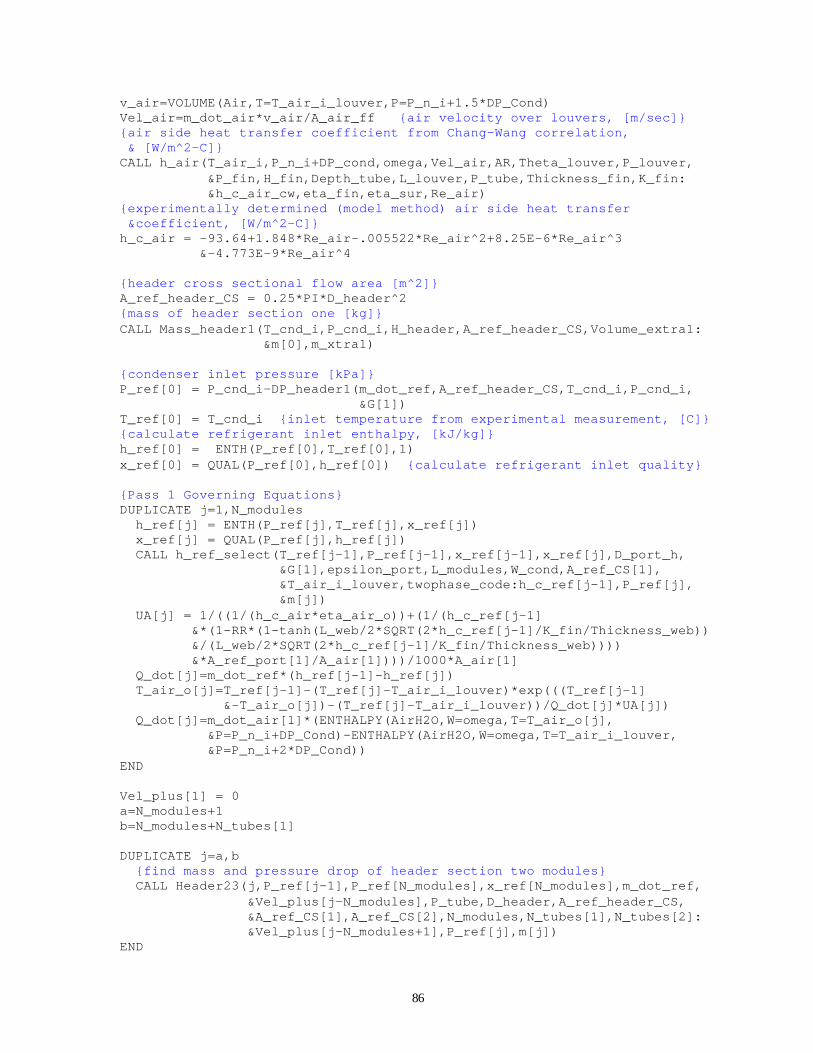
86
v_air=VOLUME(Air,T=T_air_i_louver,P=P_n_i+1.5*DP_Cond) Vel_air=m_dot_air*v_air/A_air_ff {air velocity over louvers, [m/sec]} {air side heat transfer coefficient from Chang-Wang correlation, & [W/m^2-C]} CALL h_air(T_air_i,P_n_i+DP_cond,omega,Vel_air,AR,Theta_louver,P_louver, &P_fin,H_fin,Depth_tube,L_louver,P_tube,Thickness_fin,K_fin: &h_c_air_cw,eta_fin,eta_sur,Re_air) {experimentally determined (model method) air side heat transfer &coefficient, [W/m^2-C]} h_c_air = -93.64+1.848*Re_air-.005522*Re_air^2+8.25E-6*Re_air^3 &-4.773E-9*Re_air^4 {header cross sectional flow area [m^2]} A_ref_header_CS = 0.25*PI*D_header^2 {mass of header section one [kg]} CALL Mass_header1(T_cnd_i,P_cnd_i,H_header,A_ref_header_CS,Volume_extra1: &m[0],m_xtra1) {condenser inlet pressure [kPa]} P_ref[0] = P_cnd_i-DP_header1(m_dot_ref,A_ref_header_CS,T_cnd_i,P_cnd_i, &G[1]) T_ref[0] = T_cnd_i {inlet temperature from experimental measurement, [C]} {calculate refrigerant inlet enthalpy, [kJ/kg]} h_ref[0] = ENTH(P_ref[0],T_ref[0],1) x_ref[0] = QUAL(P_ref[0],h_ref[0]) {calculate refrigerant inlet quality} {Pass 1 Governing Equations} DUPLICATE j=1,N_modules h_ref[j] = ENTH(P_ref[j],T_ref[j],x_ref[j]) x_ref[j] = QUAL(P_ref[j],h_ref[j]) CALL h_ref_select(T_ref[j-1],P_ref[j-1],x_ref[j-1],x_ref[j],D_port_h, &G[1],epsilon_port,L_modules,W_cond,A_ref_CS[1], &T_air_i_louver,twophase_code:h_c_ref[j-1],P_ref[j], &m[j]) UA[j] = 1/((1/(h_c_air*eta_air_o))+(1/(h_c_ref[j-1] &*(1-RR*(1-tanh(L_web/2*SQRT(2*h_c_ref[j-1]/K_fin/Thickness_web)) &/(L_web/2*SQRT(2*h_c_ref[j-1]/K_fin/Thickness_web)))) &*A_ref_port[1]/A_air[1])))/1000*A_air[1] Q_dot[j]=m_dot_ref*(h_ref[j-1]-h_ref[j]) T_air_o[j]=T_ref[j-1]-(T_ref[j]-T_air_i_louver)*exp(((T_ref[j-1] &-T_air_o[j])-(T_ref[j]-T_air_i_louver))/Q_dot[j]*UA[j]) Q_dot[j]=m_dot_air[1]*(ENTHALPY(AirH2O,W=omega,T=T_air_o[j], &P=P_n_i+DP_Cond)-ENTHALPY(AirH2O,W=omega,T=T_air_i_louver, &P=P_n_i+2*DP_Cond)) END Vel_plus[1] = 0 a=N_modules+1 b=N_modules+N_tubes[1] DUPLICATE j=a,b {find mass and pressure drop of header section two modules} CALL Header23(j,P_ref[j-1],P_ref[N_modules],x_ref[N_modules],m_dot_ref, &Vel_plus[j-N_modules],P_tube,D_header,A_ref_header_CS, &A_ref_CS[1],A_ref_CS[2],N_modules,N_tubes[1],N_tubes[2]: &Vel_plus[j-N_modules+1],P_ref[j],m[j]) END
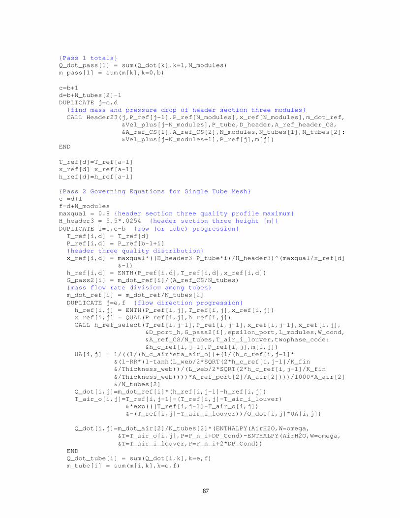
87
{Pass 1 totals} Q_dot_pass[1] = sum(Q_dot[k],k=1,N_modules) m_pass[1] = sum(m[k],k=0,b) c=b+1 d=b+N_tubes[2]-1 DUPLICATE j=c,d {find mass and pressure drop of header section three modules} CALL Header23(j,P_ref[j-1],P_ref[N_modules],x_ref[N_modules],m_dot_ref, &Vel_plus[j-N_modules],P_tube,D_header,A_ref_header_CS, &A_ref_CS[1],A_ref_CS[2],N_modules,N_tubes[1],N_tubes[2]: &Vel_plus[j-N_modules+1],P_ref[j],m[j]) END T_ref[d]=T_ref[a-1] x_ref[d]=x_ref[a-1] h_ref[d]=h_ref[a-1] {Pass 2 Governing Equations for Single Tube Mesh} e =d+1 f=d+N_modules maxqual = 0.8 {header section three quality profile maximum} H_header3 = 5.5*.0254 {header section three height [m]} DUPLICATE i=1,e-b {row (or tube) progression} T_ref[i,d] = T_ref[d] P_ref[i,d] = P_ref[b-1+i] {header three quality distribution} x_ref[i,d] = maxqual*((H_header3-P_tube*i)/H_header3)^(maxqual/x_ref[d] &-1) h_ref[i,d] = ENTH(P_ref[i,d],T_ref[i,d],x_ref[i,d]) G_pass2[i] = m_dot_ref[i]/(A_ref_CS/N_tubes) {mass flow rate division among tubes} m_dot_ref[i] = m_dot_ref/N_tubes[2] DUPLICATE j=e,f {flow direction progression} h_ref[i,j] = ENTH(P_ref[i,j],T_ref[i,j],x_ref[i,j]) x_ref[i,j] = QUAL(P_ref[i,j],h_ref[i,j]) CALL h_ref_select(T_ref[i,j-1],P_ref[i,j-1],x_ref[i,j-1],x_ref[i,j], &D_port_h,G_pass2[i],epsilon_port,L_modules,W_cond, &A_ref_CS/N_tubes,T_air_i_louver,twophase_code: &h_c_ref[i,j-1],P_ref[i,j],m[i,j]) UA[i,j] = 1/((1/(h_c_air*eta_air_o))+(1/(h_c_ref[i,j-1]* &(1-RR*(1-tanh(L_web/2*SQRT(2*h_c_ref[i,j-1]/K_fin &/Thickness_web))/(L_web/2*SQRT(2*h_c_ref[i,j-1]/K_fin &/Thickness_web))))*A_ref_port[2]/A_air[2])))/1000*A_air[2] &/N_tubes[2] Q_dot[i,j]=m_dot_ref[i]*(h_ref[i,j-1]-h_ref[i,j]) T_air_o[i,j]=T_ref[i,j-1]-(T_ref[i,j]-T_air_i_louver) &*exp(((T_ref[i,j-1]-T_air_o[i,j]) &-(T_ref[i,j]-T_air_i_louver))/Q_dot[i,j]*UA[i,j]) Q_dot[i,j]=m_dot_air[2]/N_tubes[2]*(ENTHALPY(AirH2O,W=omega, &T=T_air_o[i,j],P=P_n_i+DP_Cond)-ENTHALPY(AirH2O,W=omega, &T=T_air_i_louver,P=P_n_i+2*DP_Cond)) END Q_dot_tube[i] = sum(Q_dot[i,k],k=e,f) m_tube[i] = sum(m[i,k],k=e,f)
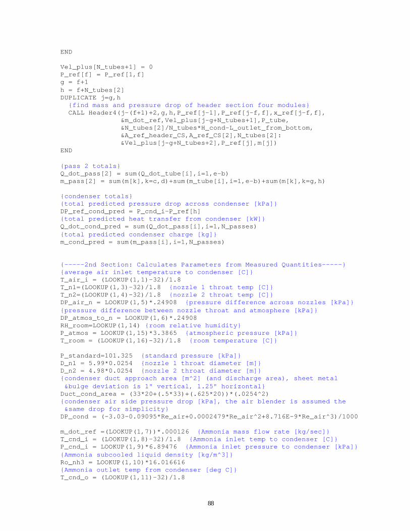
88
END Vel_plus[N_tubes+1] = 0 P_ref[f] = P_ref[1,f] g = f+1 h = f+N_tubes[2] DUPLICATE j=g,h {find mass and pressure drop of header section four modules} CALL Header4(j-(f+1)+2,g,h,P_ref[j-1],P_ref[j-f,f],x_ref[j-f,f], &m_dot_ref,Vel_plus[j-g+N_tubes+1],P_tube, &N_tubes[2]/N_tubes*H_cond-L_outlet_from_bottom, &A_ref_header_CS,A_ref_CS[2],N_tubes[2]: &Vel_plus[j-g+N_tubes+2],P_ref[j],m[j]) END {pass 2 totals} Q_dot_pass[2] = sum(Q_dot_tube[i],i=1,e-b) m_pass[2] = sum(m[k],k=c,d)+sum(m_tube[i],i=1,e-b)+sum(m[k],k=g,h) {condenser totals} {total predicted pressure drop across condenser [kPa]} DP_ref_cond_pred = P_cnd_i-P_ref[h] {total predicted heat transfer from condenser [kW]} Q_dot_cond_pred = sum(Q_dot_pass[i],i=1,N_passes) {total predicted condenser charge [kg]} m_cond_pred = sum(m_pass[i],i=1,N_passes) {-----2nd Section: Calculates Parameters from Measured Quantities-----} {average air inlet temperature to condenser [C]} T_air_i = (LOOKUP(1,1)-32)/1.8 T_n1=(LOOKUP(1,3)-32)/1.8 {nozzle 1 throat temp [C]} T_n2=(LOOKUP(1,4)-32)/1.8 {nozzle 2 throat temp [C]} DP_air_n = LOOKUP(1,5)*.24908 {pressure difference across nozzles [kPa]} {pressure difference between nozzle throat and atmosphere [kPa]} DP_atmos_to_n = LOOKUP(1,6)*.24908 RH_room=LOOKUP(1,14) {room relative humidity} P_atmos = LOOKUP(1,15)*3.3865 {atmospheric pressure [kPa]} T_room = (LOOKUP(1,16)-32)/1.8 {room temperature [C]} P_standard=101.325 {standard pressure [kPa]} D_n1 = 5.99*0.0254 {nozzle 1 throat diameter [m]} D_n2 = 4.98*0.0254 {nozzle 2 throat diameter [m]} {condenser duct approach area [m^2] (and discharge area), sheet metal &bulge deviation is 1" vertical, 1.25" horizontal} Duct_cond_area = (33*20+(.5*33)+(.625*20))*(.0254^2) {condenser air side pressure drop [kPa], the air blender is assumed the &same drop for simplicity} DP_cond = (-3.03-0.09095*Re_air+0.0002479*Re_air^2+8.716E-9*Re_air^3)/1000 m_dot_ref =(LOOKUP(1,7))*.000126 {Ammonia mass flow rate [kg/sec]} T_cnd_i = (LOOKUP(1,8)-32)/1.8 {Ammonia inlet temp to condenser [C]} P_cnd_i = LOOKUP(1,9)*6.89476 {Ammonia inlet pressure to condenser [kPa]} {Ammonia subcooled liquid density [kg/m^3]} Ro_nh3 = LOOKUP(1,10)*16.016616 {Ammonia outlet temp from condenser [deg C]} T_cnd_o = (LOOKUP(1,11)-32)/1.8
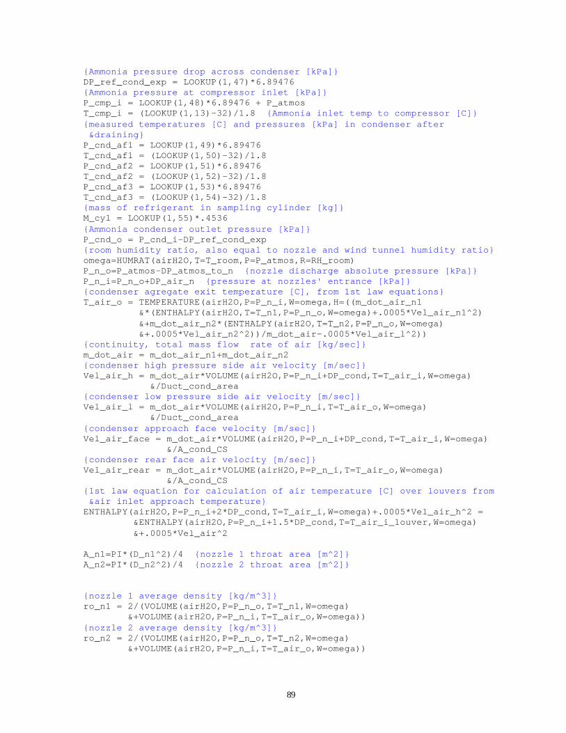
89
{Ammonia pressure drop across condenser [kPa]} DP_ref_cond_exp = LOOKUP(1,47)*6.89476 {Ammonia pressure at compressor inlet [kPa]} P_cmp_i = LOOKUP(1,48)*6.89476 + P_atmos T_cmp_i = (LOOKUP(1,13)-32)/1.8 {Ammonia inlet temp to compressor [C]} {measured temperatures [C] and pressures [kPa] in condenser after &draining} P_cnd_af1 = LOOKUP(1,49)*6.89476 T_cnd_af1 = (LOOKUP(1,50)-32)/1.8 P_cnd_af2 = LOOKUP(1,51)*6.89476 T_cnd_af2 = (LOOKUP(1,52)-32)/1.8 P_cnd_af3 = LOOKUP(1,53)*6.89476 T_cnd_af3 = (LOOKUP(1,54)-32)/1.8 {mass of refrigerant in sampling cylinder [kg]} M_cyl = LOOKUP(1,55)*.4536 {Ammonia condenser outlet pressure [kPa]} P_cnd_o = P_cnd_i-DP_ref_cond_exp {room humidity ratio, also equal to nozzle and wind tunnel humidity ratio} omega=HUMRAT(airH2O,T=T_room,P=P_atmos,R=RH_room) P_n_o=P_atmos-DP_atmos_to_n {nozzle discharge absolute pressure [kPa]} P_n_i=P_n_o+DP_air_n {pressure at nozzles' entrance [kPa]} {condenser agregate exit temperature [C], from 1st law equations} T_air_o = TEMPERATURE(airH2O,P=P_n_i,W=omega,H=((m_dot_air_n1 &*(ENTHALPY(airH2O,T=T_n1,P=P_n_o,W=omega)+.0005*Vel_air_n1^2) &+m_dot_air_n2*(ENTHALPY(airH2O,T=T_n2,P=P_n_o,W=omega) &+.0005*Vel_air_n2^2))/m_dot_air-.0005*Vel_air_l^2)) {continuity, total mass flow rate of air [kg/sec]} m_dot_air = m_dot_air_n1+m_dot_air_n2 {condenser high pressure side air velocity [m/sec]} Vel_air_h = m_dot_air*VOLUME(airH2O,P=P_n_i+DP_cond,T=T_air_i,W=omega) &/Duct_cond_area {condenser low pressure side air velocity [m/sec]} Vel_air_l = m_dot_air*VOLUME(airH2O,P=P_n_i,T=T_air_o,W=omega) &/Duct_cond_area {condenser approach face velocity [m/sec]} Vel_air_face = m_dot_air*VOLUME(airH2O,P=P_n_i+DP_cond,T=T_air_i,W=omega) &/A_cond_CS {condenser rear face air velocity [m/sec]} Vel_air_rear = m_dot_air*VOLUME(airH2O,P=P_n_i,T=T_air_o,W=omega) &/A_cond_CS {1st law equation for calculation of air temperature [C] over louvers from &air inlet approach temperature} ENTHALPY(airH2O,P=P_n_i+2*DP_cond,T=T_air_i,W=omega)+.0005*Vel_air_h^2 = &ENTHALPY(airH2O,P=P_n_i+1.5*DP_cond,T=T_air_i_louver,W=omega) &+.0005*Vel_air^2 A_n1=PI*(D_n1^2)/4 {nozzle 1 throat area [m^2]} A_n2=PI*(D_n2^2)/4 {nozzle 2 throat area [m^2]} {nozzle 1 average density [kg/m^3]} ro_n1 = 2/(VOLUME(airH2O,P=P_n_o,T=T_n1,W=omega) &+VOLUME(airH2O,P=P_n_i,T=T_air_o,W=omega)) {nozzle 2 average density [kg/m^3]} ro_n2 = 2/(VOLUME(airH2O,P=P_n_o,T=T_n2,W=omega) &+VOLUME(airH2O,P=P_n_i,T=T_air_o,W=omega))
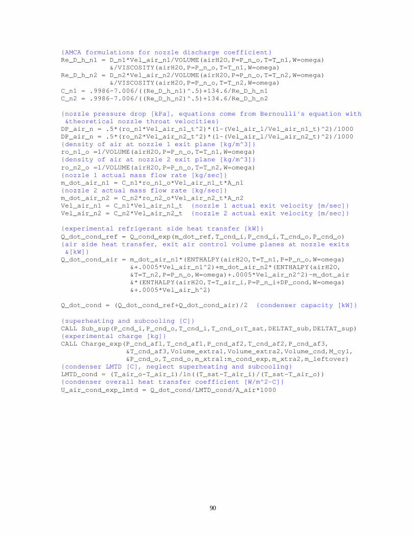
90
{AMCA formulations for nozzle discharge coefficient} Re_D_h_n1 = D_n1*Vel_air_n1/VOLUME(airH2O,P=P_n_o,T=T_n1,W=omega) &/VISCOSITY(airH2O,P=P_n_o,T=T_n1,W=omega) Re_D_h_n2 = D_n2*Vel_air_n2/VOLUME(airH2O,P=P_n_o,T=T_n2,W=omega) &/VISCOSITY(airH2O,P=P_n_o,T=T_n2,W=omega) C_n1 = .9986-7.006/((Re_D_h_n1)^.5)+134.6/Re_D_h_n1 C_n2 = .9986-7.006/((Re_D_h_n2)^.5)+134.6/Re_D_h_n2 {nozzle pressure drop [kPa], equations come from Bernoulli's equation with &theoretical nozzle throat velocities} DP_air_n = .5*(ro_n1*Vel_air_n1_t^2)*(1-(Vel_air_l/Vel_air_n1_t)^2)/1000 DP_air_n = .5*(ro_n2*Vel_air_n2_t^2)*(1-(Vel_air_l/Vel_air_n2_t)^2)/1000 {density of air at nozzle 1 exit plane [kg/m^3]} ro_n1_o =1/VOLUME(airH2O,P=P_n_o,T=T_n1,W=omega) {density of air at nozzle 2 exit plane [kg/m^3]} ro_n2_o =1/VOLUME(airH2O,P=P_n_o,T=T_n2,W=omega) {nozzle 1 actual mass flow rate [kg/sec]} m_dot_air_n1 = C_n1*ro_n1_o*Vel_air_n1_t*A_n1 {nozzle 2 actual mass flow rate [kg/sec]} m_dot_air_n2 = C_n2*ro_n2_o*Vel_air_n2_t*A_n2 Vel_air_n1 = C_n1*Vel_air_n1_t {nozzle 1 actual exit velocity [m/sec]} Vel_air_n2 = C_n2*Vel_air_n2_t {nozzle 2 actual exit velocity [m/sec]} {experimental refrigerant side heat transfer [kW]} Q_dot_cond_ref = Q_cond_exp(m_dot_ref,T_cnd_i,P_cnd_i,T_cnd_o,P_cnd_o) {air side heat transfer, exit air control volume planes at nozzle exits &[kW]} Q_dot_cond_air = m_dot_air_n1*(ENTHALPY(airH2O,T=T_n1,P=P_n_o,W=omega) &+.0005*Vel_air_n1^2)+m_dot_air_n2*(ENTHALPY(airH2O, &T=T_n2,P=P_n_o,W=omega)+.0005*Vel_air_n2^2)-m_dot_air &*(ENTHALPY(airH2O,T=T_air_i,P=P_n_i+DP_cond,W=omega) &+.0005*Vel_air_h^2) Q_dot_cond = (Q_dot_cond_ref+Q_dot_cond_air)/2 {condenser capacity [kW]} {superheating and subcooling [C]} CALL Sub_sup(P_cnd_i,P_cnd_o,T_cnd_i,T_cnd_o:T_sat,DELTAT_sub,DELTAT_sup) {experimental charge [kg]} CALL Charge_exp(P_cnd_af1,T_cnd_af1,P_cnd_af2,T_cnd_af2,P_cnd_af3, &T_cnd_af3,Volume_extra1,Volume_extra2,Volume_cnd,M_cyl, &P_cnd_o,T_cnd_o,m_xtra1:m_cond_exp,m_xtra2,m_leftover) {condenser LMTD [C], neglect superheating and subcooling} LMTD_cond = (T_air_o-T_air_i)/ln((T_sat-T_air_i)/(T_sat-T_air_o)) {condenser overall heat transfer coefficient [W/m^2-C]} U_air_cond_exp_lmtd = Q_dot_cond/LMTD_cond/A_air*1000

91
Appendix E: Experimental Setup Components
This Appendix contains photographs of the experimental setup and technical details of the evaporator
and compressor.
Figure E.1: Serpentine Condenser
Figure E.2: Microchannel Condenser with Air Exit Thermocouple Grid
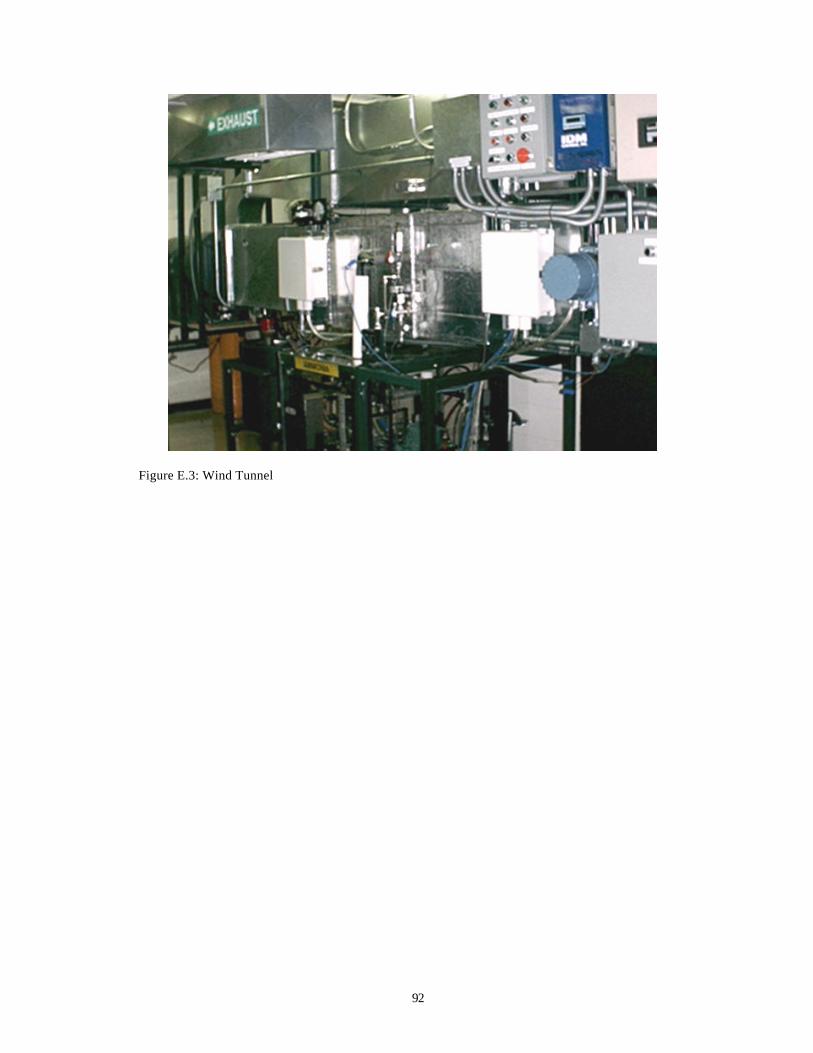
92
Figure E.3: Wind Tunnel
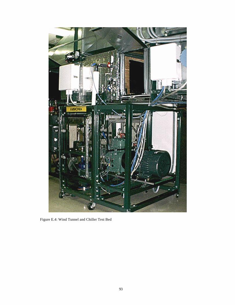
93
Figure E.4: Wind Tunnel and Chiller Test Bed
94
Figure E.5: Wind Tunnel and Chiller Test Bed, Alternate View
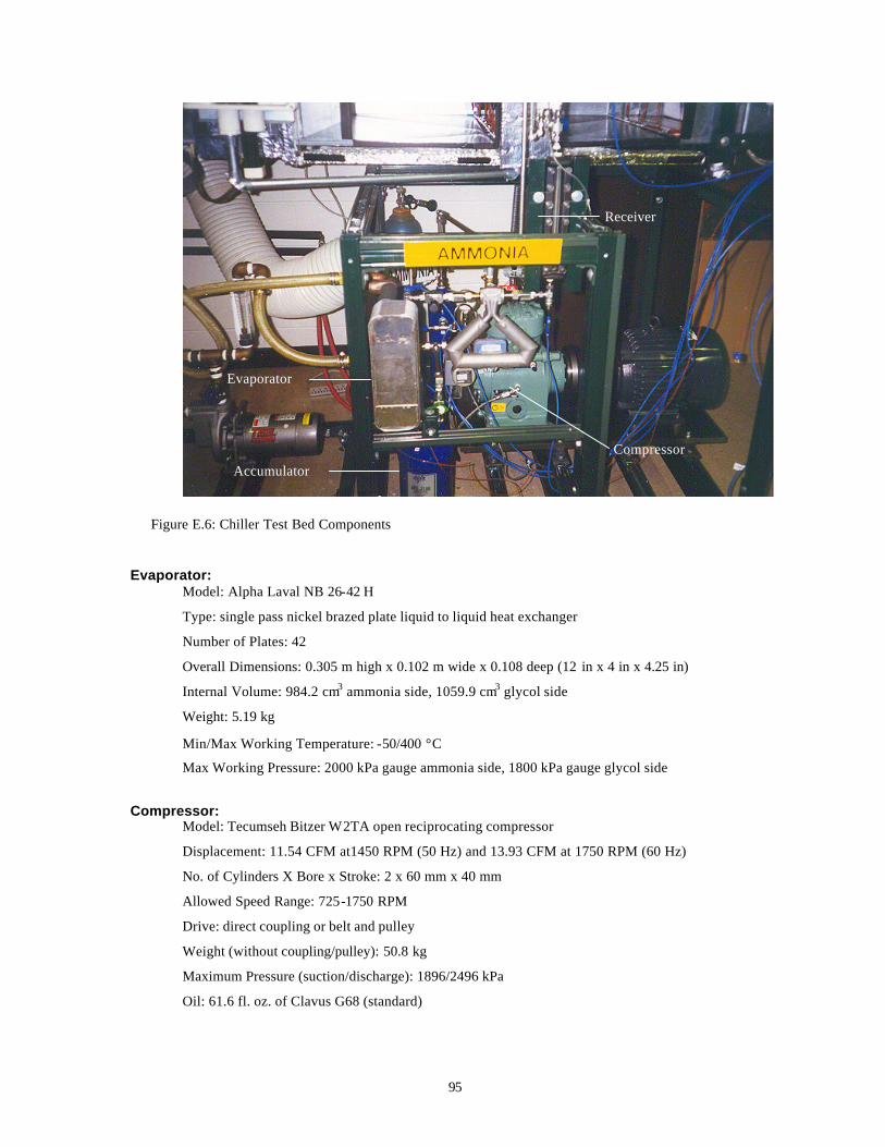
95
Figure E.6: Chiller Test Bed Components
Evaporator: Model: Alpha Laval NB 26-42 H
Type: single pass nickel brazed plate liquid to liquid heat exchanger
Number of Plates: 42
Overall Dimensions: 0.305 m high x 0.102 m wide x 0.108 deep (12 in x 4 in x 4.25 in)
Internal Volume: 984.2 cm3 ammonia side, 1059.9 cm3 glycol side
Weight: 5.19 kg
Min/Max Working Temperature: -50/400 °C
Max Working Pressure: 2000 kPa gauge ammonia side, 1800 kPa gauge glycol side
Compressor: Model: Tecumseh Bitzer W2TA open reciprocating compressor
Displacement: 11.54 CFM at1450 RPM (50 Hz) and 13.93 CFM at 1750 RPM (60 Hz)
No. of Cylinders X Bore x Stroke: 2 x 60 mm x 40 mm
Allowed Speed Range: 725-1750 RPM
Drive: direct coupling or belt and pulley
Weight (without coupling/pulley): 50.8 kg
Maximum Pressure (suction/discharge): 1896/2496 kPa
Oil: 61.6 fl. oz. of Clavus G68 (standard)
Compressor
Accumulator
Evaporator
Receiver

96
List of References
Achaichia, A. and Cowell, T.A. 1988. “Heat Transfer and Pressure Drop Characteristics of Flat Tube and Louvered Plated Fin Surfaces.” Experimental Thermal Fluid Science 1: 147-157.
Butterworth, D. 1975. “A Comparison of Some Void -Fraction Relationships for Co-Current Gas-Liquid Flow.” International Journal of Multiphase Flow, 1: 845-850.
Chang, Y-J and Wang, C-C. 1996a. “A Generalized Heat Transfer Correlation for Louver Fin Geometry.” Int. J. Heat Mass Transfer 40: 533-544.
Chang, Y-J and Wang, C-C. 1996b. “Air Side Performance of Brazed Aluminum Heat Exchangers.” Journal of Enhanced Heat Transfer (3)1: 15-28.
Churchill, S.W. 1977. “Friction-Factor Equation Spans all Fluid-Flow Regimes.” Chemical Engineering November 7: 91-92.
Davenport, C.J. 1983. “Correlation for Heat Transfer and Flow Friction Characteristics of Louvered Fins.” AIChE Symp. Ser. 79(25): 19-27.
de Souza, A.M. and Pimenta, M.M. 1995. “Prediction of Pressure Drop During Horizontal Two-Phase Flow of Pure and Mixed Refrigerants.” ASME Cavitation and Multiphase Flow 210: 161-171.
Dobson, M.K. and Chato, J.C. 1998. “Condensation in Smooth Horizontal Tubes.” ASME Journal of Heat Transfer 120: 193-213.
Gnielinski, V. 1976. “New Equations for Heat and Mass Transfer in Turbulent Pipe and Channel Flow.” International Chemical Engineering 16(2): 359-368.
Heun, M.K. and Dunn, W.E. 1995. Performance and Optimization of Microchannel Condensers. ACRC TR-81, University of Illinois.
Heun, M.K. and Dunn, W.E. 1996. “Principles of Refrigerant Circuiting with Application to Microchannel Condensers.” ASHRAE Transactions: Symposia. 2: 373-393.
Hughmark, G.A. “Holdup in Gas-Liquid Flow.” Chemical Engineering Progress. 58(4): 62-65
Idelchik, I.E. 1994. Handbook of Hydraulic Resistance. 3rd ed. CRC Press, Inc. Boca Raton, FL.
Incropera, F.P. and DeWitt, D.P. 1996. Fundamentals of Heat and Mass Transfer. 4th ed. John Wiley & Sons. New York.
Kays, W.M. and London, A.L. 1998. Compact Heat Exchangers. 3rd ed. Krieger Publishing Co. Malabar, FL.
Newell, T.A. et al. 1999. “An Investigation of Void Fraction in the Stratified/Annular Flow Regions in Smooth, Horizontal Tubes.” In Review for International Journal of Multiphase Flow.
Shah, M.M. 1978. “A General Correlation for Heat Transfer During Film Condensation Inside Pipes.” International Journal of Heat and Mass Transfer 22: 547-556.
Soliman, H.M. 1982. “On the Annular-to-Wavy Flow Pattern Transition During Condensation Inside Horizontal Tubes.” The Canadian Journal of Chemical Engineering 60: 475-481.
White, F.M. 1986. Fluid Mechanics. McGraw-Hill, Inc. New York
Zietlow, D.C. and Pedersen, C.O. 1995. Heat Transfer and Flow Characteristics of Condensing Refrigerants in Small-channel Crossflow Heat Exchangers. ACRC TR-73, Un iversity of Illinois.
Zivi, S.M. 1964. “Estimation of Steady-State Steam Void -Fraction by Means of the Principle of Minimum Entropy Production.” ASME Journal of Heat Transfer 86: 247-252.
Recommended