Computing for Data Sciences
Lecture 4
Introduction:
The Singular value decomposition (SVD) is a factorization of a real or complex matrix. It has
many useful applications in signal processing and statistics. Formally, the singular value
decomposition of an m × n real or complex matrix M is a factorization of the form 𝑀 = 𝑈𝛴𝑉!,
where U is an m × m real or complex unitary matrix, Σ is an m × n rectangular diagonal
matrix with non-negative real numbers on the diagonal, and 𝑉! (the conjugate transpose of V, or
simply the transpose of V if V is real) is an n × n real or complex unitary matrix. The diagonal
entries 𝛴!,! of Σ are known as the singular values of M. The m columns of U and the n columns
of V are called the left-singular vectors and right-singular vectors of M, respectively.
SVD is primarily used for dimension reduction which is converting data of very high
dimensionality into data of much lower dimensionality such that each of the lower dimensions
convey much more information.
Consider an example:
Suppose you have a list of 100 movies and 1000 people and for each person, you know whether
they like or dislike each of the 100 movies. So for each instance (which in this case means each
person) you have a binary vector of length 100 (position i is 0 if that person dislikes the i'th
movie, otherwise 1.
You can perform your machine learning task on these vectors directly.. but instead you could
decide upon 5 genres of movies and using the data you already have, figure out whether the
person likes or dislikes the entire genre and, in this way reduce your data from a vector of size
100 into a vector of size 5 [position i is 1 if the person likes genre i]
The vector of length 5 can be thought of as a good representative of the vector of length 100
because most people might be liking movies only in their preferred genres. Though this may not
be an exact representation since there will be people who might hate all the 5 genres but the rest
of them more or less can be confined using this method.
This is mainly done because the reduced vector conveys most of the information in the larger one
while consuming a lot less space and being faster to compute with.
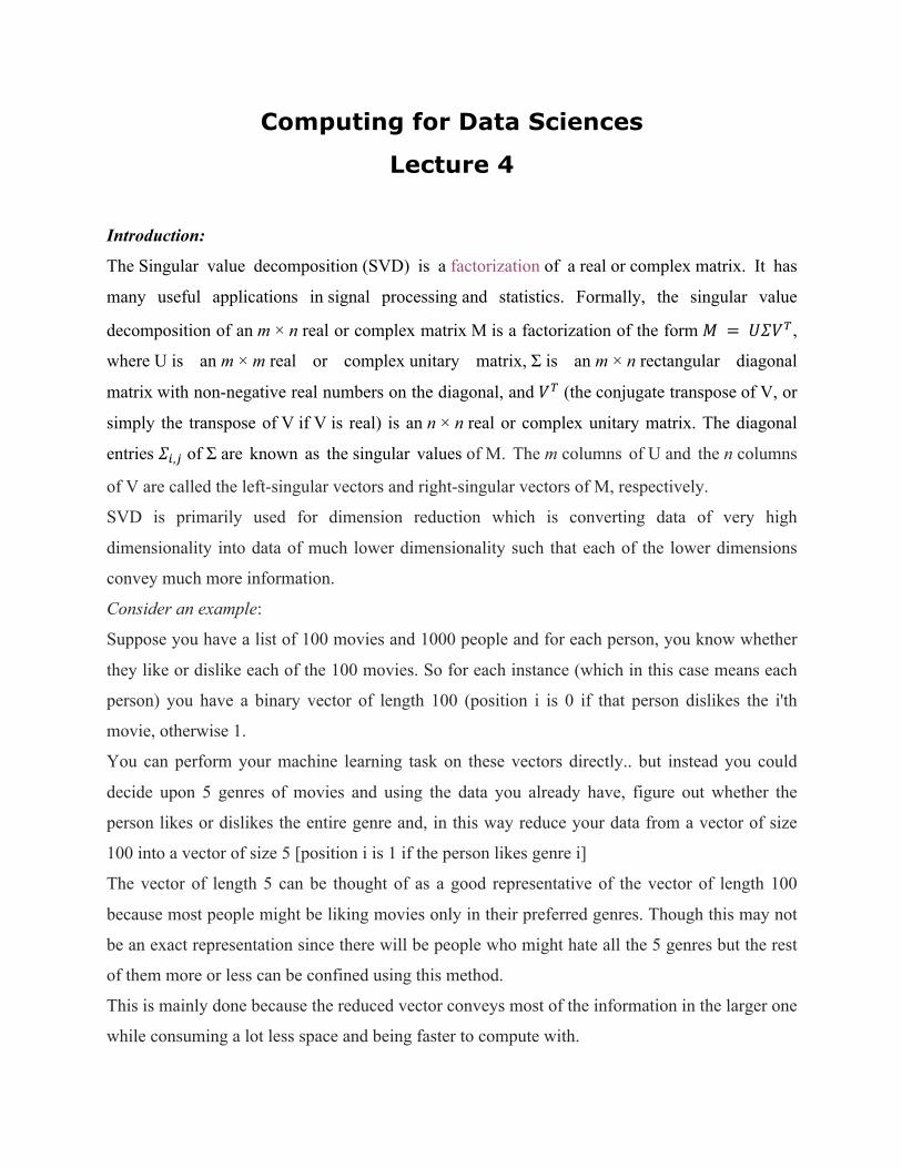
Figure 1. Fundamental picture of Linear Algebra
Fig.1 is used to explain the equation Ax = b. The first step sees Ax (matrix times vector) as a
combination of the columns of A. Those vectors Ax fill the column space C (A). When we move
from one combination to all combinations (by allowing every x), a subspace appears. Ax = b has
a solution exactly when b is in the column space of A
NOTE: We choose a matrix of rank one, = 𝑥𝑦! . When 𝑚 = 𝑛 = 2, all four fundamental
subspaces are lines in ℝ!
The dimensions obey the most important laws of linear algebra: 𝑑𝑖𝑚 𝑅(𝐴) = 𝑑𝑖𝑚 𝑅(𝐴!) and
𝑑𝑖𝑚 𝑅(𝐴) + 𝑑𝑖𝑚 𝑁(𝐴) = 𝑛.
The row space has dimension 𝑟, the nullspace has dimension 𝑛 − 𝑟. Elimination identifies r
pivot variables and 𝑛 − 𝑟 free variables. Those variables correspond, in the echelon form, to
columns with pivots and columns without pivots. They give the dimension count 𝑟 and 𝑛 – 𝑟.
Every 𝑥 in the nullspace is perpendicular to every row of the matrix, exactly because 𝐴𝑥 = 0

Fig.2
From Fig.2 we can see that 𝐴 takes 𝑥 into the column space, nullspace goes to the zero vector.
Nothing goes elsewhere in the left nullspace. With 𝑏 in the column space, 𝐴𝑥 = 𝑏 can be
solved. There is a particular solution 𝑥, in the row space. The homogeneous solutions 𝑥, forms
the nullspace. The general solution is 𝑥! + 𝑥!. The particularity of 𝑥! is that it is orthogonal to
every 𝑥!.
Visualizing the Fundamental Picture of Linear Algebra in terms of different types of Matrices.
• Matrices which behave as Injective function (1 to 1).

In the above figure it can be seen that all the elements of Row space of A map to Column space
of A. There is only one element in C(AT) which maps to zero. There is no null space of A, only
there is zero in Row space of A that maps to zero.
• Matrices which behave as Surjective function (Onto).
In the above picture it can be seen that the null space of AT does not exists. This ensures that the
range of matrix we are considering does not have any element that can be mapped from
• Matrices which behave as Bijective function (Onto).
The span of a finite, non-empty set of vectors {u1, u2, ... , un} is the set of all possible linear
combinations of those vectors, i.e. the set of all vectors of the form c1u1 + c2u2 + ... + cnun for
some scalars c1, c2, ..., cn.

The three vectors E1, E2, E3 present in R2 span the
whole R2 . This can be represented as
Span{E1,E2,E3}= R2
The vectors E1,E2,E3 can be the representation of the
space R2. We don’t need all the three vectors to represent
our space. The space R2 can be spanned by 2 vectors
either E1, E2 or E2, E3 or E1, E3.
Span{E1,E2}= R2 Span{E2,E3}= R2 Span{E1,E3}= R2
This type of representation where only n-linearly independent vectors map the n-dimensional
vector space is know is Minimal Representation. The minimum set of vectors that span the
space are called Basis. ex {E1,E2} ,{E2,E3}.
A basis of a vector space is defined as a subset of vectors in that are linearly
independent and vector space span . Consequently, if is a list of vectors in ,
then these vectors form a basis if and only if every can be uniquely written as
where , ..., are scalars. A vector space will have many different bases, but there is always
the same number of basis vectors in each of them. The number of basis vectors in is called
the dimension of . Every spanning list in a vector space can be reduced to a basis of the vector
space. The bases need not be orthogonal to each other they must be linearly independent.
Greedy Approach of finding bases of Vector
The greedy approach involves picking n linearly independent vectors such that they are linearly
independent. These vectors can be the basis of n dimensional space. There are two types of
greedy Algorithm for finding bases of vectors.
Grow Algorithm

The algorithm stops when there is no vector to add, at which time S spans all of V. Thus, if the
algorithm stops, it will have found a generating set.
Shrink Algorithm
The algorithm stops when there is no vector whose removal would leave a spanning set. At every
point during the algorithm, S spans V, so it spans V at the end. Thus, if the algorithm stops, the
algorithm will have found a generating set.
Choice by Induction Approach of finding bases of Vector
Method 1: Pick a basis 11 ℜ∈B and then 22 ℜ∈B Such that )1(2 BSpanB ∉ . Then pick a basis 33 ℜ∈B such that )2,1(3 BBSpanB ∉ . Then proceed in similar manner to find the other basis.
Finally find the nBn ℜ∈ such that )1,...2,1( −∉ BnBBSpanBn .
Method 2: Pick a vector Bi such that Bi is orthogonal to all the bases vector selected before it
(B1, B2... Bi-‐1). This will ensure that all the vectors are linearly independent. Being orthogonal
means the inner product of two vectors is zero. 01, =BBi 02, =BBi ........ 01, =−BiBi
The orthonormal basis vectors means, the basis vectors are orthogonal and their size=1, i.e their
norm=1. 11 =B , 12 =B , 13 =B ..... 1=Bn
Representation of basis vectors produced by the above two methods.
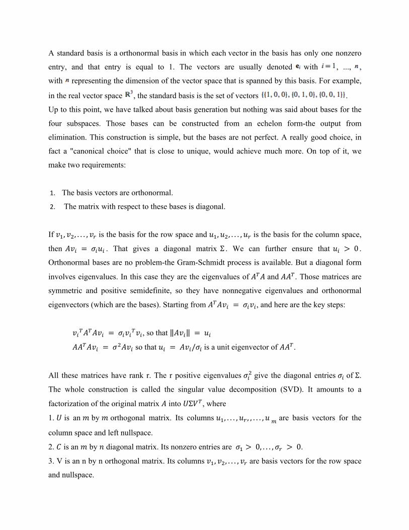
A standard basis is a orthonormal basis in which each vector in the basis has only one nonzero
entry, and that entry is equal to 1. The vectors are usually denoted with , ..., ,
with representing the dimension of the vector space that is spanned by this basis. For example,
in the real vector space , the standard basis is the set of vectors .
Up to this point, we have talked about basis generation but nothing was said about bases for the
four subspaces. Those bases can be constructed from an echelon form-the output from
elimination. This construction is simple, but the bases are not perfect. A really good choice, in
fact a "canonical choice" that is close to unique, would achieve much more. On top of it, we
make two requirements:
1. The basis vectors are orthonormal.
2. The matrix with respect to these bases is diagonal.
If 𝑣!, 𝑣!, . . . , 𝑣! is the basis for the row space and 𝑢!,𝑢!, . . . ,𝑢! is the basis for the column space,
then 𝐴𝑣! = 𝜎!𝑢! . That gives a diagonal matrix Σ . We can further ensure that 𝑢! > 0 .
Orthonormal bases are no problem-the Gram-Schmidt process is available. But a diagonal form
involves eigenvalues. In this case they are the eigenvalues of 𝐴!𝐴 and 𝐴𝐴!. Those matrices are
symmetric and positive semidefinite, so they have nonnegative eigenvalues and orthonormal
eigenvectors (which are the bases). Starting from 𝐴!𝐴𝑣! = 𝜎!𝑣!, and here are the key steps:
𝑣!!𝐴!𝐴𝑣! = 𝜎!𝑣!!𝑣!, so that 𝐴𝑣! = 𝑢!
𝐴𝐴!𝐴𝑣! = 𝜎!𝐴𝑣! so that 𝑢! = 𝐴𝑣!/𝜎! is a unit eigenvector of 𝐴𝐴!.
All these matrices have rank r. The r positive eigenvalues 𝜎!! give the diagonal entries 𝜎! of Σ.
The whole construction is called the singular value decomposition (SVD). It amounts to a
factorization of the original matrix 𝐴 into 𝑈Σ𝑉!, where
1. 𝑈 is an 𝑚 by 𝑚 orthogonal matrix. Its columns 𝑢!, . . . ,𝑢! , , . . . ,𝑢 ! are basis vectors for the
column space and left nullspace.
2. 𝐶 is an 𝑚 by 𝑛 diagonal matrix. Its nonzero entries are 𝜎! > 0, . . . ,𝜎! > 0.
3. V is an n by n orthogonal matrix. Its columns 𝑣!, 𝑣!, . . . , 𝑣! are basis vectors for the row space
and nullspace.
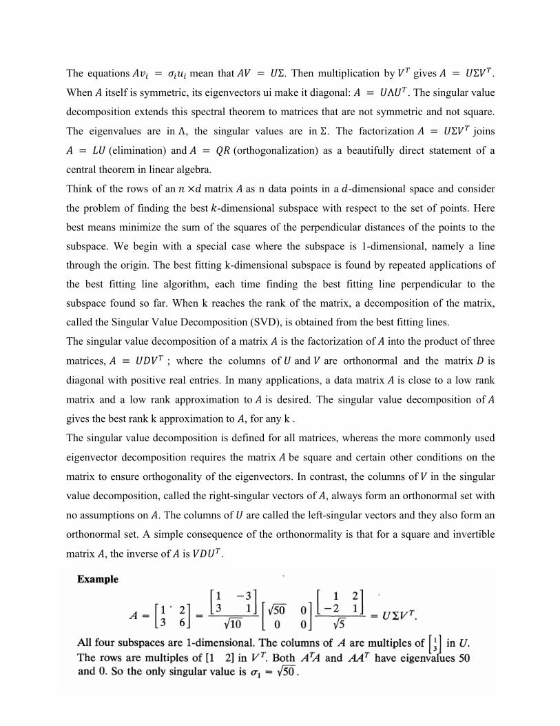
The equations 𝐴𝑣! = 𝜎!𝑢! mean that 𝐴𝑉 = 𝑈Σ. Then multiplication by 𝑉! gives 𝐴 = 𝑈Σ𝑉!.
When 𝐴 itself is symmetric, its eigenvectors ui make it diagonal: 𝐴 = 𝑈Λ𝑈!. The singular value
decomposition extends this spectral theorem to matrices that are not symmetric and not square.
The eigenvalues are in Λ, the singular values are in Σ. The factorization 𝐴 = 𝑈Σ𝑉! joins
𝐴 = 𝐿𝑈 (elimination) and 𝐴 = 𝑄𝑅 (orthogonalization) as a beautifully direct statement of a
central theorem in linear algebra.
Think of the rows of an 𝑛 ×𝑑 matrix 𝐴 as n data points in a 𝑑-dimensional space and consider
the problem of finding the best 𝑘-dimensional subspace with respect to the set of points. Here
best means minimize the sum of the squares of the perpendicular distances of the points to the
subspace. We begin with a special case where the subspace is 1-dimensional, namely a line
through the origin. The best fitting k-dimensional subspace is found by repeated applications of
the best fitting line algorithm, each time finding the best fitting line perpendicular to the
subspace found so far. When k reaches the rank of the matrix, a decomposition of the matrix,
called the Singular Value Decomposition (SVD), is obtained from the best fitting lines.
The singular value decomposition of a matrix 𝐴 is the factorization of 𝐴 into the product of three
matrices, 𝐴 = 𝑈𝐷𝑉! ; where the columns of 𝑈 and 𝑉 are orthonormal and the matrix 𝐷 is
diagonal with positive real entries. In many applications, a data matrix 𝐴 is close to a low rank
matrix and a low rank approximation to 𝐴 is desired. The singular value decomposition of 𝐴
gives the best rank k approximation to 𝐴, for any k .
The singular value decomposition is defined for all matrices, whereas the more commonly used
eigenvector decomposition requires the matrix 𝐴 be square and certain other conditions on the
matrix to ensure orthogonality of the eigenvectors. In contrast, the columns of 𝑉 in the singular
value decomposition, called the right-singular vectors of 𝐴, always form an orthonormal set with
no assumptions on 𝐴. The columns of 𝑈 are called the left-singular vectors and they also form an
orthonormal set. A simple consequence of the orthonormality is that for a square and invertible
matrix 𝐴, the inverse of 𝐴 is 𝑉𝐷𝑈!.

Figure: Orthonormal bases that diagonalize 𝐴.
Factorizations of Matrices:
By bringing together three important ways to factor the matrix A, we can find solutions to
various problems.
1. PLU Factorization
Here,
P is a so-called permutation matrix, L is lower triangular, U is upper triangular.
We will start with LU Factorisation:
LU-Factorization:- The nonsingular matrix A has an LU-factorization if it can be expressed as
the product of a lower-triangular matrix L and an upper triangular matrix U:
𝐴 = 𝐿𝑈
Condition for factorization: square matrix A
Permutation Matrix:
A permutation σ on {1, . . . ,𝑛} has an associated permutation matrix
So if we look at our σ = {2, 4, 1, 3}, we get matrix
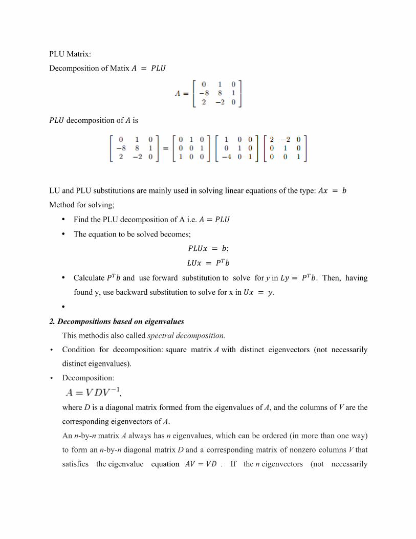
PLU Matrix:
Decomposition of Matix 𝐴 = 𝑃𝐿𝑈
𝑃𝐿𝑈 decomposition of 𝐴 is
LU and PLU substitutions are mainly used in solving linear equations of the type: 𝐴𝑥 = 𝑏
Method for solving;
• Find the PLU decomposition of A i.e. 𝐴 = 𝑃𝐿𝑈
• The equation to be solved becomes;
𝑃𝐿𝑈𝑥 = 𝑏;
𝐿𝑈𝑥 = 𝑃!𝑏
• Calculate 𝑃!𝑏 and use forward substitution to solve for y in 𝐿𝑦 = 𝑃!𝑏. Then, having
found y, use backward substitution to solve for x in 𝑈𝑥 = 𝑦.
•
2. Decompositions based on eigenvalues
This methodis also called spectral decomposition.
• Condition for decomposition: square matrix A with distinct eigenvectors (not necessarily
distinct eigenvalues).
• Decomposition:
,
where D is a diagonal matrix formed from the eigenvalues of A, and the columns of V are the
corresponding eigenvectors of A.
An n-by-n matrix A always has n eigenvalues, which can be ordered (in more than one way)
to form an n-by-n diagonal matrix D and a corresponding matrix of nonzero columns V that
satisfies the eigenvalue equation 𝐴𝑉 = 𝑉𝐷 . If the n eigenvectors (not necessarily

eigenvalues) are distinct (that is, none is equal to any of the others), then V is invertible,
implying the decomposition 𝐴 = 𝑉𝐷𝑉!!.
• One can always normalize the eigenvectors to have length one (see definition of the
eigenvalue equation). If is real-symmetric, is always invertible and can be made to
have normalized columns. Then the equation holds, because each eigenvector is
orthogonal to the other. Therefore the decomposition (which always exists if A is real-
symmetric) reads as:
• The condition of having n distinct eigenvalues is sufficient but not necessary. The necessary
and sufficient condition is for each eigenvalue to have geometric multiplicity equal to its
algebraic multiplicity.
• The eigen decomposition is useful for understanding the solution of a system of linear
ordinary differential equations or linear difference equations. For example, the difference
equation starting from the initial condition is solved by ,
which is equivalent to , where V and D are the matrices formed from the
eigenvectors and eigen values of A. Since D is diagonal, raising it to power , just involves
raising each element on the diagonal to the power t. This is much easier to do and to
understand than raising A to power t, since A is usually not diagonal.
3. Factorization of the original matrix 𝑨 into 𝑼∑𝑽𝑻
Where,
i. 𝑈 is an 𝑚 by 𝑚 orthogonal matrix. Its columns 𝑢!, . . . ,𝑢! , , . . . ,𝑢 ! are basis vectors
for the column space and left null space.
ii. ∑ is an m by n diagonal matrix. Its nonzero entries are σ1 > 0, . . . , σr > 0.
iii. V is an n by n orthogonal matrix. Its columns 𝑣!, . . , 𝑣! , . . . , 𝑣! are basis vectors for
the row space and null space.
This factorization gives us good bases for the subspaces and a ∑ matrix that provides
information about the most significance action of A.

Diagonalisation effect of A
This figure shows the diagonalization of A. Basis vectors go to .basis vectors (principal axes). A
circle goes to an ellipse. The matrix is factored into 𝑈∑𝑉!
1. VT rotates the basis vectors and brings them to the axes.
2. The ∑- singular value matrix scales the matrix primarily in the direction of principle
component, making it look like an ellipsoid. The stretching along each axes is independent of the
other.
3. 𝑈 matrix is an orthonormal basis matrix. It provides the effect of rotation in its own way. This
operation does not provide any scaling effect.
Recommended