Computer Networks: Computer Networks: RoutingRouting
11
Network LayerNetwork Layer
Routing
Computer Networks: Computer Networks: RoutingRouting
22
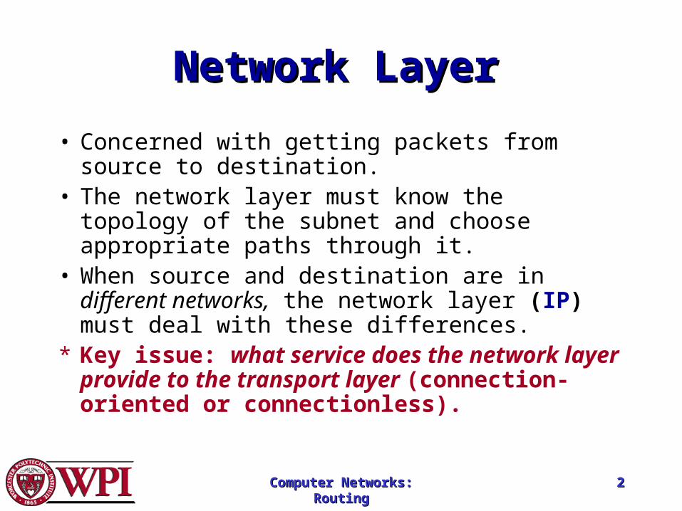
Network LayerNetwork Layer
• Concerned with getting packets from source to destination.
• The network layer must know the topology of the subnet and choose appropriate paths through it.
• When source and destination are in different networks, the network layer (IP) must deal with these differences.
* Key issue: what service does the network layer provide to the transport layer (connection-oriented or connectionless).
Computer Networks: Computer Networks: RoutingRouting
33
Network Layer Design Network Layer Design GoalsGoals
1. The services provided by the network layer should be independent of the subnet topology.
2. The Transport Layer should be shielded from the number, type and topology of the subnets present.
3. The network addresses available to the Transport Layer should use a uniform numbering plan (even across LANs and WANs).
Computer Networks: Computer Networks: RoutingRouting
44
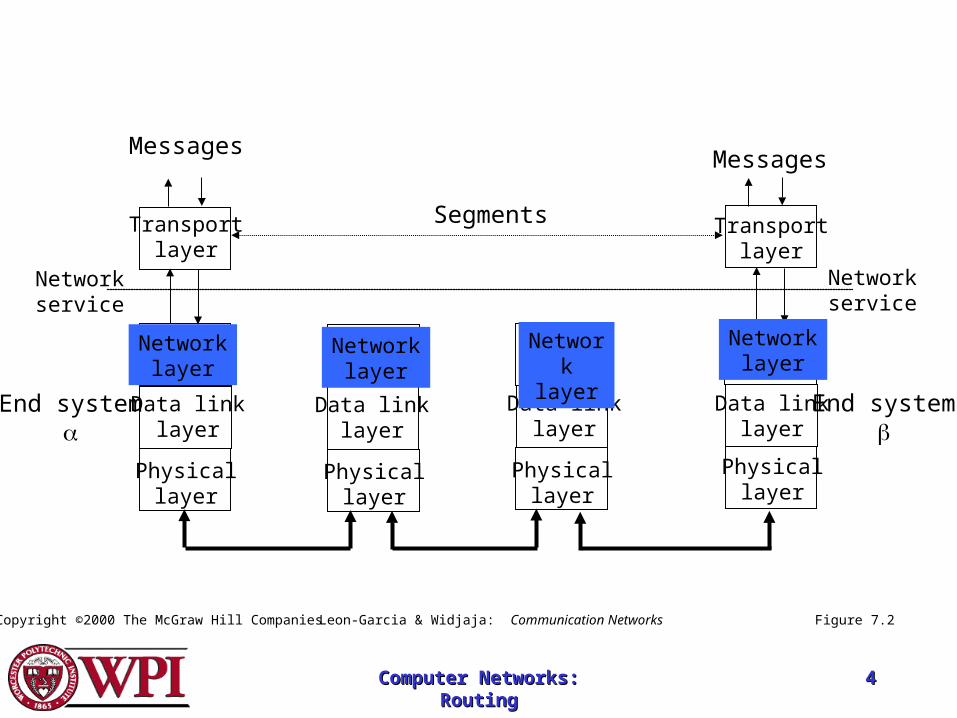
Figure 7.2
Physicallayer
Data linklayer
Physicallayer
Data linklayer
End system
Networklayer
Physicallayer
Data linklayer
Physicallayer
Data linklayer
Transportlayer
Transportlayer
MessagesMessages
Segments
End system
Networkservice
Networkservice
Copyright ©2000 The McGraw Hill Companies Leon-Garcia & Widjaja: Communication Networks
Networklayer
Networklayer
Networklayer
Computer Networks: Computer Networks: RoutingRouting
55
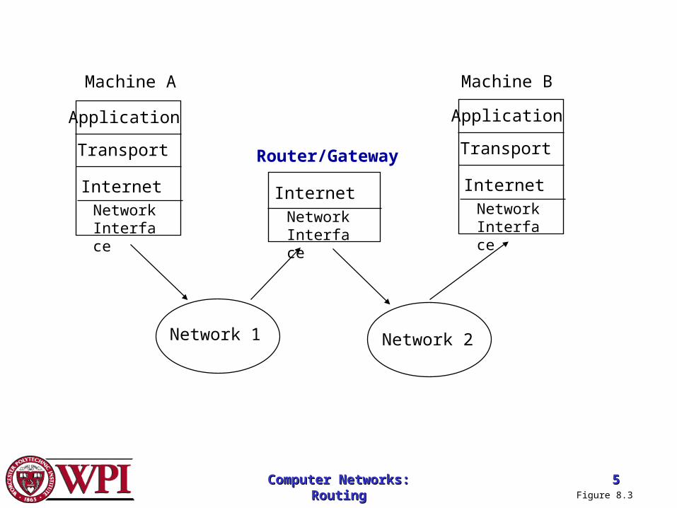
Application
Transport
InternetNetwork Interface
Application
Transport
InternetInternet
Network 1 Network 2
Machine A Machine B
Router/Gateway
Network Interface
Network Interface
Figure 8.3
Computer Networks: Computer Networks: RoutingRouting
66
RR
RR
S
SS
s
s s
s
ss
s
ss
s
R
s
R
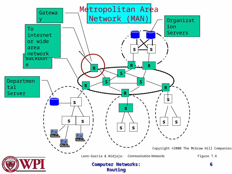
Backbone
To internet or wide area network
Organization Servers
Gateway
Departmental Server
Figure 7.6
Copyright ©2000 The McGraw Hill Companies
Leon-Garcia & Widjaja: Communication Networks
Metropolitan AreaNetwork (MAN)
Computer Networks: Computer Networks: RoutingRouting
77
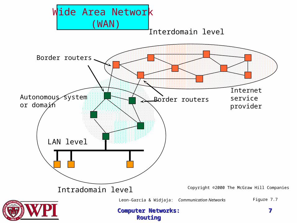
Interdomain level
Intradomain level
LAN level
Autonomous systemor domain
Border routers
Border routers
Figure 7.7
Internet service provider
Copyright ©2000 The McGraw Hill Companies
Leon-Garcia & Widjaja: Communication Networks
Wide Area Network (WAN)
Computer Networks: Computer Networks: RoutingRouting
88
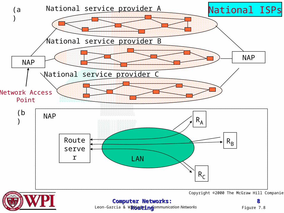
RA
RB
RC
Route server
NAP
National service provider A
National service provider B
National service provider C
LAN
NAPNAP
(a)
(b)
Figure 7.8
Copyright ©2000 The McGraw Hill Companies
Leon-Garcia & Widjaja: Communication Networks
National ISPs
Network AccessPoint
Computer Networks: Computer Networks: RoutingRouting
99
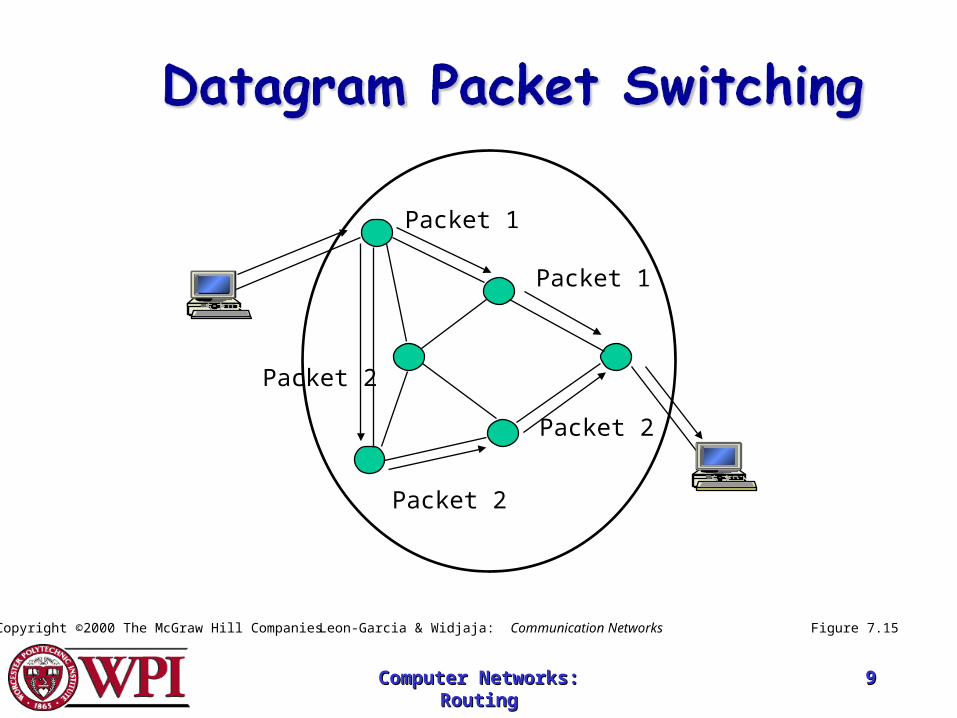
Packet 2
Packet 1
Packet 1
Packet 2
Packet 2
Figure 7.15Copyright ©2000 The McGraw Hill Companies Leon-Garcia & Widjaja: Communication Networks
Computer Networks: Computer Networks: RoutingRouting
1010
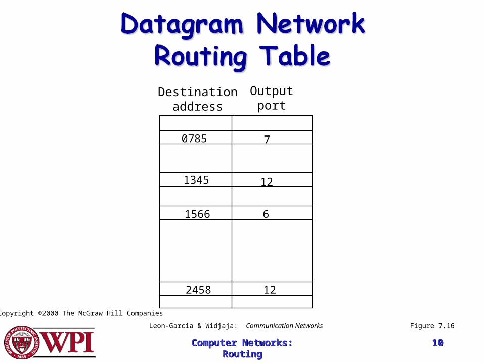
Destinationaddress
Outputport
1345 12
2458
70785
6
12
1566
Figure 7.16
Copyright ©2000 The McGraw Hill Companies
Leon-Garcia & Widjaja: Communication Networks
Computer Networks: Computer Networks: RoutingRouting
1111
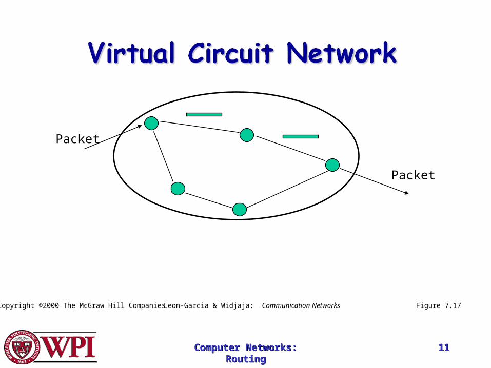
Packet
Packet
Figure 7.17Copyright ©2000 The McGraw Hill Companies Leon-Garcia & Widjaja: Communication Networks
Computer Networks: Computer Networks: RoutingRouting
1212
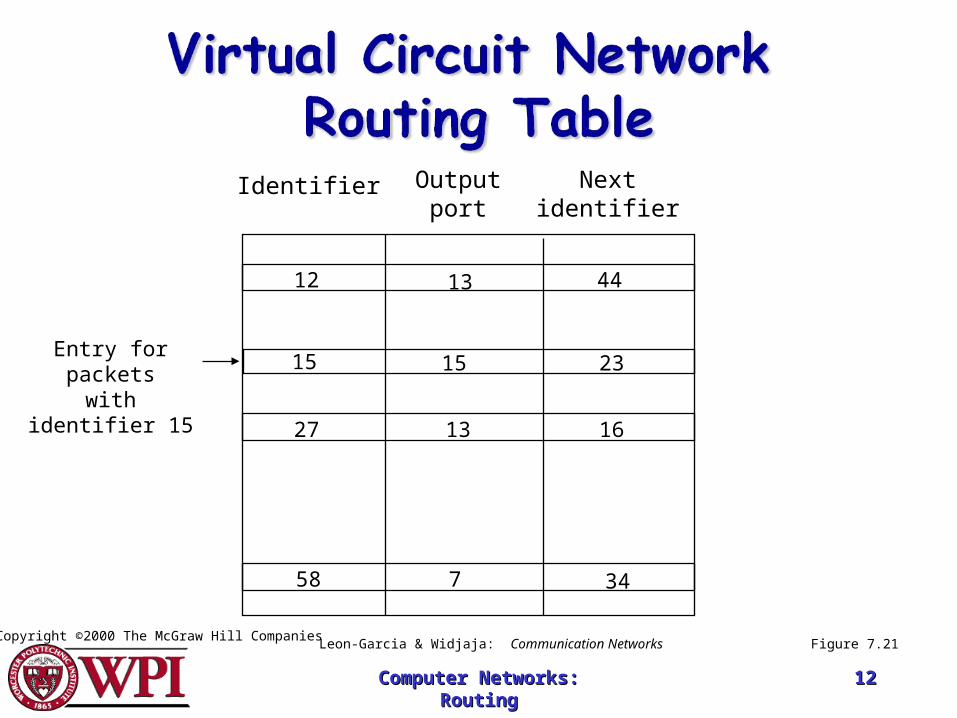
Identifier Outputport
15 15
58
13
13
7
27
12
Nextidentifier
44
23
16
34
Entry for packetswith identifier 15
Figure 7.21Copyright ©2000 The McGraw Hill Companies
Leon-Garcia & Widjaja: Communication Networks
Computer Networks: Computer Networks: RoutingRouting
1313
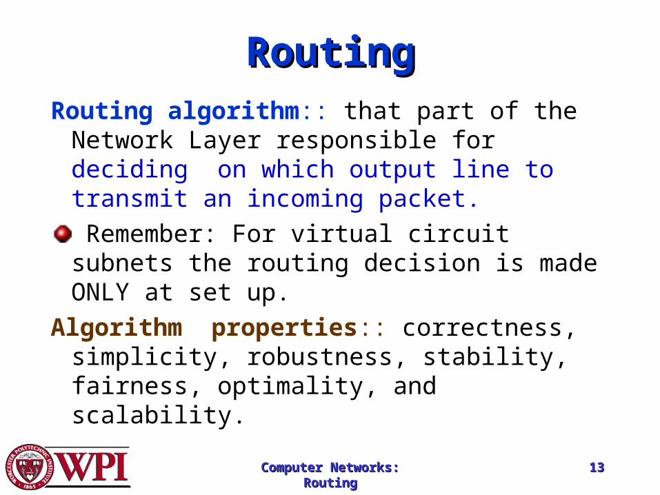
RoutingRoutingRouting algorithm:: that part of the
Network Layer responsible for deciding on which output line to transmit an incoming packet. Remember: For virtual circuit subnets the routing decision is made ONLY at set up.
Algorithm properties:: correctness, simplicity, robustness, stability, fairness, optimality, and scalability.
Computer Networks: Computer Networks: RoutingRouting
1414
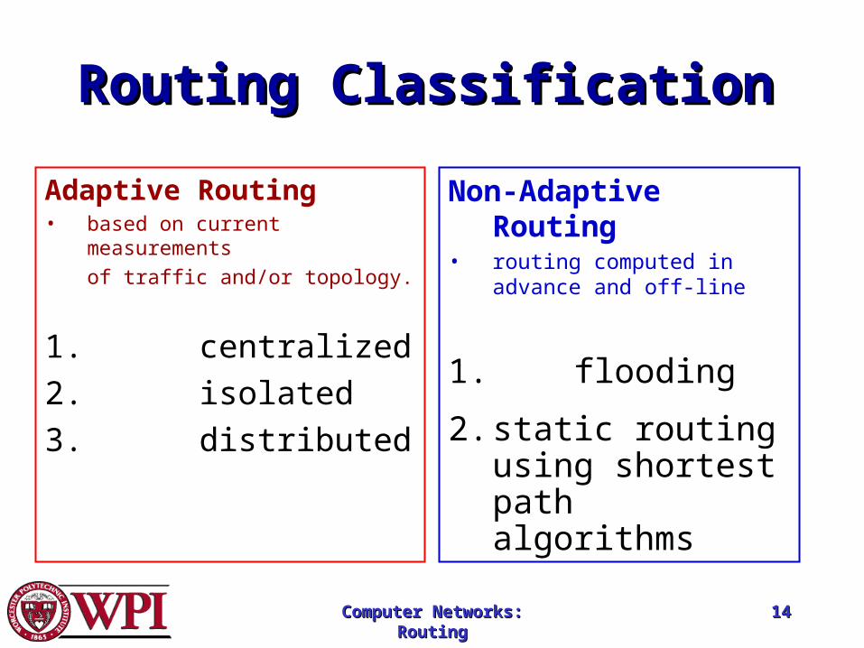
Routing ClassificationRouting Classification
Adaptive Routing• based on current measurements
of traffic and/or topology.
1. centralized
2. isolated
3. distributed
Non-Adaptive Routing• routing computed in advance
and off-line
1. flooding
2. static routing using shortest path algorithms
Computer Networks: Computer Networks: RoutingRouting
1515
FloodingFlooding• Pure flooding :: every incoming packet to a
node is sent out on every outgoing line.– Obvious adjustment – do not send out on
arriving link (assuming full-duplex links).– The routing algorithm can use a hop counter
(e.g., TTL) to dampen the flooding.– Selective flooding :: only send on those
lines going “approximately” in the right direction.
Computer Networks: Computer Networks: RoutingRouting
1616
Shortest Path RoutingShortest Path Routing
1. Bellman-Ford Algorithm [Distance Vector]2. Dijkstra’s Algorithm [Link State]
What does it mean to be the shortest (or optimal) route?
Choices:a. Minimize the number of hops along the path.b. Minimize mean packet delay.c. Maximize the network throughput.
Computer Networks: Computer Networks: RoutingRouting
1717
Possible MetricsPossible Metrics
• Set all link costs to 1.– Shortest hop routing.– Disregards delay and capacity differences on
links!
{Original ARPANET}• Measure the number of packets queued to
be transmitted on each link.– Did not work well.
Computer Networks: Computer Networks: RoutingRouting
1818
MetricsMetrics{Second ARPANET}
• Timestamp each arriving packet with its ArrivalTime and record DepartTime* and use link-level ACK to compute:
Delay = (DepartTime – ArrivalTime) + TransmissionTime + Latency
• The weight assigned to each link was average delay over ‘recent’ packets sent.
• This algorithm tended to oscillate – leading to idle periods and instability.
* Reset after retransmission
Computer Networks: Computer Networks: RoutingRouting
1919
MetricsMetrics
{Revised ARPANET} – Compress dynamic range of the metric to
account for link type– Smooth the variation of metric with time:
• Delay transformed into link utilization
• Utilization was then averaged with last reported utilization to deal with spikes.
• Set a hard limit on how much the metric could change per measurement cycle.
Computer Networks: Computer Networks: RoutingRouting
2020
Dijkstra’s Shortest Path AlgorithmDijkstra’s Shortest Path Algorithm
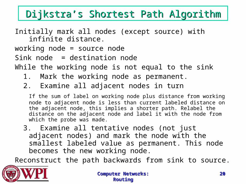
Initially mark all nodes (except source) with infinite distance.working node = source nodeSink node = destination nodeWhile the working node is not equal to the sink 1. Mark the working node as permanent. 2. Examine all adjacent nodes in turn
If the sum of label on working node plus distance from working node to adjacent node is less than current labeled distance on the adjacent node, this implies a shorter path. Relabel the distance on the adjacent node and label it with the node from which the probe was made.
3. Examine all tentative nodes (not just adjacent nodes) and mark the node with the smallest labeled value as permanent. This node becomes the new working node.
Reconstruct the path backwards from sink to source.
Computer Networks: Computer Networks: RoutingRouting
2121
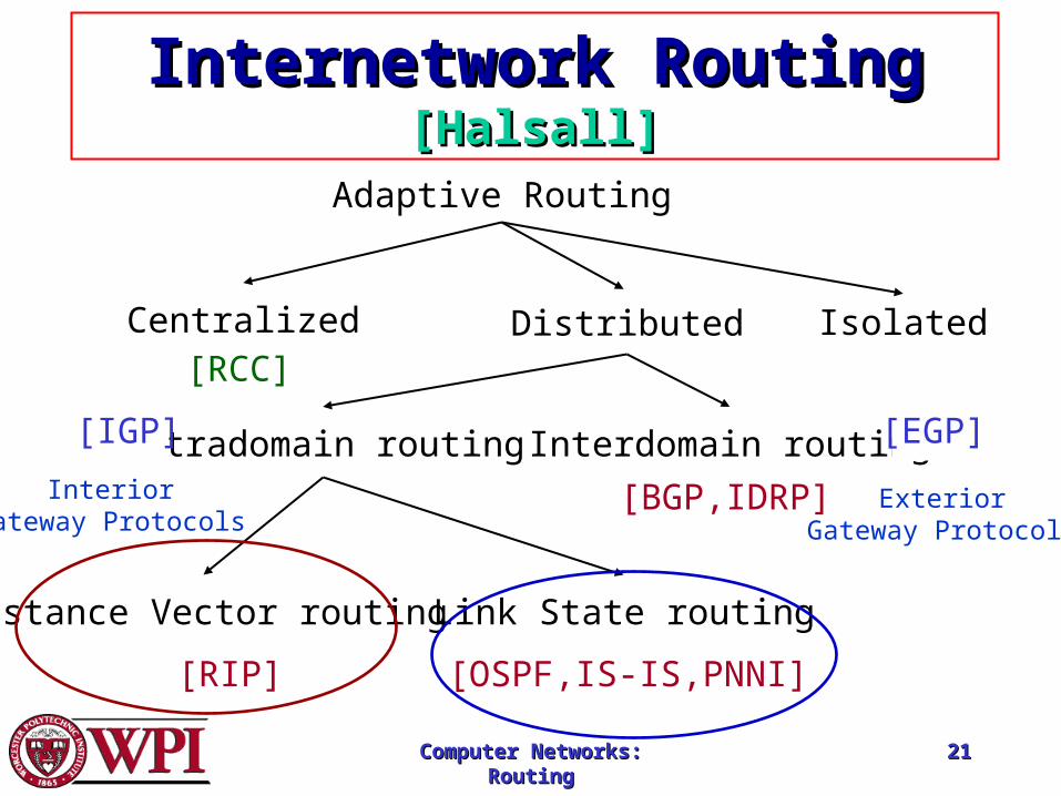
Internetwork RoutingInternetwork Routing [Halsall][Halsall]
Adaptive Routing
Centralized Distributed
Intradomain routing Interdomain routing
Distance Vector routing Link State routing
[IGP] [EGP]
[BGP,IDRP]
[OSPF,IS-IS,PNNI][RIP]
[RCC]
InteriorGateway Protocols
ExteriorGateway Protocols
Isolated
Computer Networks: Computer Networks: RoutingRouting
2222
Adaptive RoutingAdaptive RoutingDesign Issues:1. How much overhead is incurred due to
gathering the routing information and sending routing packets?
2. What is the time frame (i.e, the frequency) for sending routing packets in support of adaptive routing?
3. What is the complexity of the routing strategy?
Computer Networks: Computer Networks: RoutingRouting
2323
Adaptive RoutingAdaptive Routing
Basic functions:1. Measurement of pertinent network data.2. Forwarding of information to where the
routing computation will be done.3. Compute the routing tables.4. Convert the routing table information into
a routing decision and then dispatch the data packet.
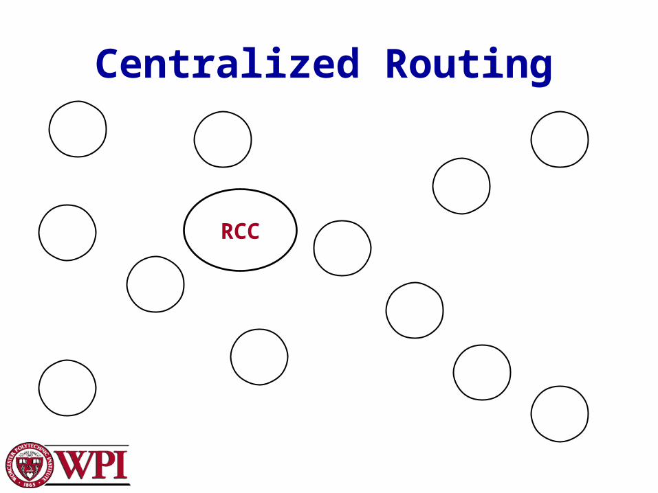
Centralized Routing
RCC
Computer Networks: Computer Networks: RoutingRouting
2525
Distance Vector Distance Vector RoutingRouting
• Historically known as the old ARPANET routing algorithm {or known as Bellman-Ford algorithm}.
Basic idea: each network node maintains a Distance Vector table containing the distance between itself and ALL possible destination nodes.
• Distances are based on a chosen metric and are computed using information from the neighbors’ distance vectors.
Metric: usually hops or delay
Computer Networks: Computer Networks: RoutingRouting
2626
Distance Vector Distance Vector RoutingRouting
Information kept by DV router
1. each router has an ID
2. associated with each link connected to a router, there is a link cost (static or dynamic).
Distance Vector Table Initialization
Distance to itself = 0
Distance to ALL other routers = infinity number
Computer Networks: Computer Networks: RoutingRouting
2727
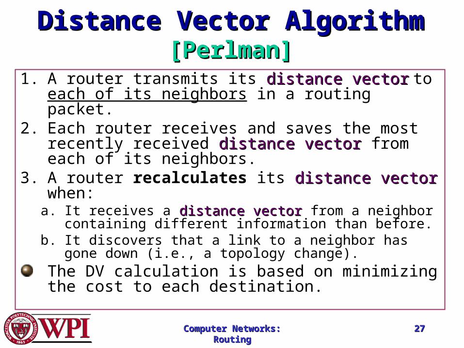
Distance Vector AlgorithmDistance Vector Algorithm [Perlman][Perlman]
1. A router transmits its distance vectordistance vector to each of its neighbors in a routing packet.
2. Each router receives and saves the most recently received distance vectordistance vector from each of its neighbors.
3. A router recalculates its distance vectordistance vector when:a. It receives a distance vectordistance vector from a neighbor
containing different information than before.b. It discovers that a link to a neighbor has gone down (i.e., a
topology change).The DV calculation is based on minimizing the cost to each destination.
Computer Networks: Computer Networks: RoutingRouting
2828
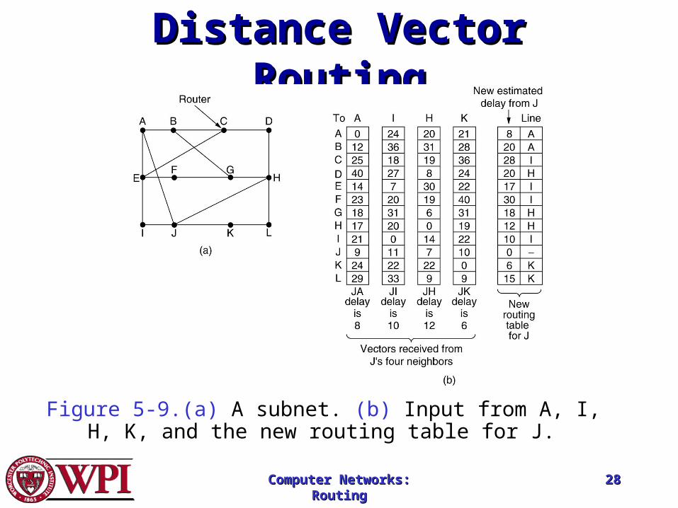
Distance Vector Distance Vector RoutingRouting
Figure 5-9.(a) A subnet. (b) Input from A, I, H, K, and the new routing table for J.
Computer Networks: Computer Networks: RoutingRouting
2929
Routing Information Routing Information Protocol (RIP)Protocol (RIP)
• RIP had widespread use because it was distributed with BSD Unix in “routed”, a router management daemon.
• RIP is the most used Distance Vector protocol.• RFC1058 in June 1988.• Sends packets every 30 seconds or faster.• Runs over UDP.• Metric = hop count• BIG problem is max. hop count =16
RIP limited to running on small networks!!• Upgraded to RIPv2
Computer Networks: Computer Networks: RoutingRouting
3030
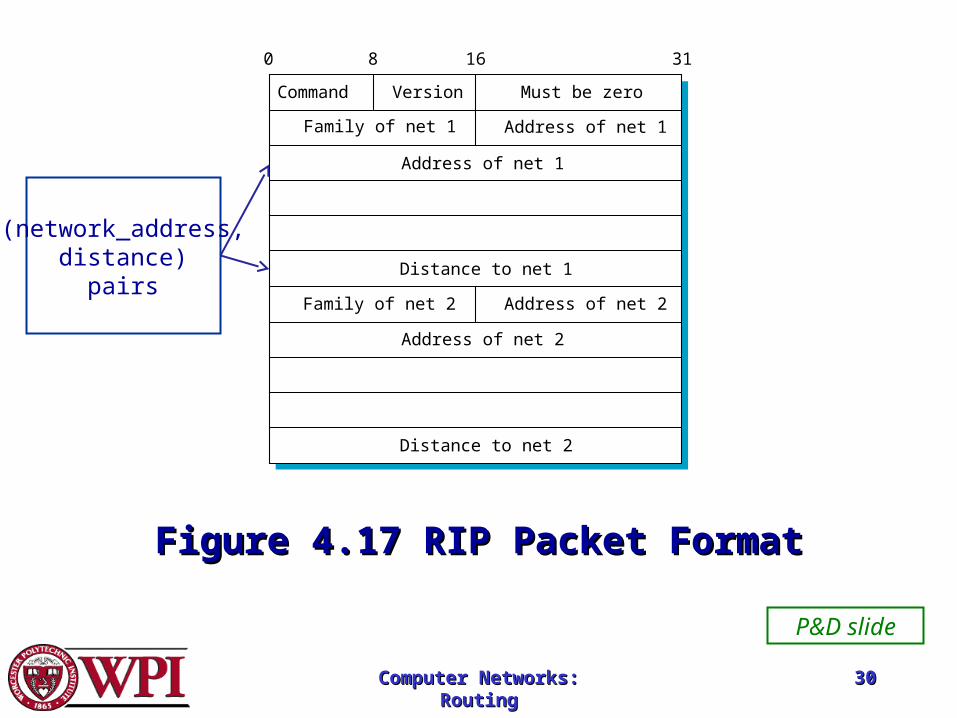
Figure 4.17 RIP Packet FormatFigure 4.17 RIP Packet Format
Address of net 2
Distance to net 2
Command Must be zero
Family of net 2 Address of net 2
Family of net 1 Address of net 1
Address of net 1
Distance to net 1
Version
0 8 16 31
(network_address,distance)
pairs
P&D slide
Computer Networks: Computer Networks: RoutingRouting
3131
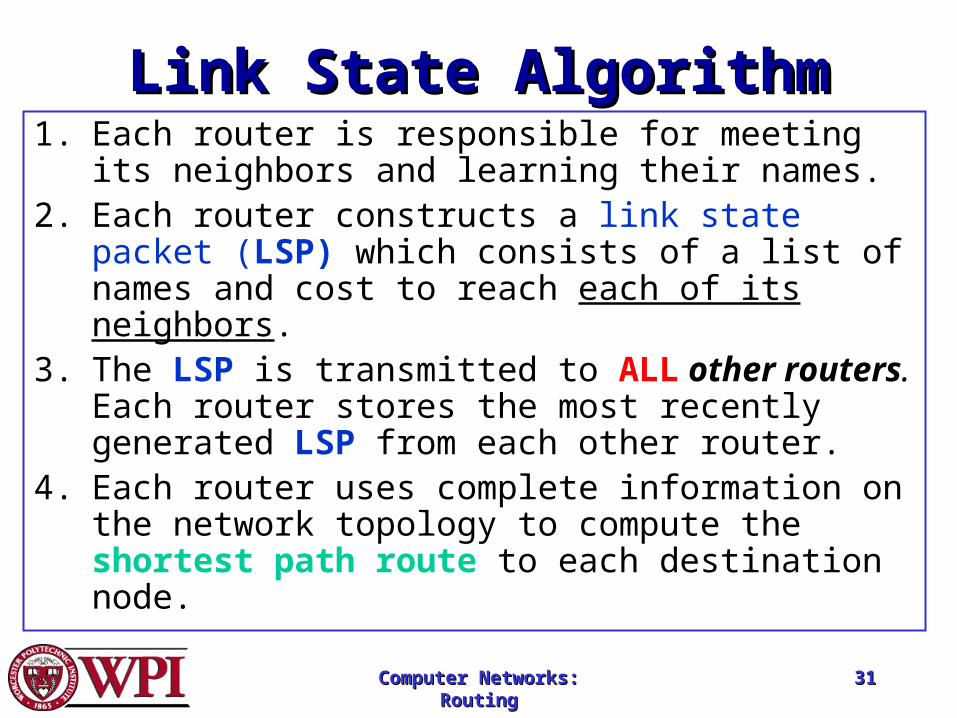
Link State AlgorithmLink State Algorithm1. Each router is responsible for meeting its neighbors
and learning their names.2. Each router constructs a link state packet (LSP) which
consists of a list of names and cost to reach each of its neighbors.
3. The LSP is transmitted to ALL other routers. Each router stores the most recently generated LSP from each other router.
4. Each router uses complete information on the network topology to compute the shortest path route to each destination node.
Computer Networks: Computer Networks: RoutingRouting
3232
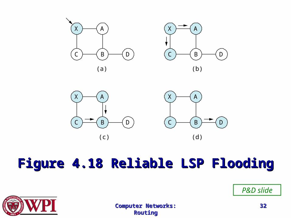
Figure 4.18 Reliable LSP FloodingFigure 4.18 Reliable LSP Flooding
(a)
X A
C B D
(b)
X A
C B D
(c)
X A
C B D
(d)
X A
C B D
P&D slide
Computer Networks: Computer Networks: RoutingRouting
3333
Reliable FloodingReliable Flooding• The process of making sure all the nodes
participating in the routing protocol get a copy of the link-state information from all the other nodes.
• LSP contains:– Sending router’s node ID– List of connected neighbors with the
associated link cost to each neighbor– Sequence number– Time-to-live (TTL)
Computer Networks: Computer Networks: RoutingRouting
3434
Reliable FloodingReliable Flooding• First two items enable route calculation
• Last two items make process reliable– ACKs and checking for duplicates is needed.
• Periodic Hello packets used to determine the demise of a neighbor.
• The sequence numbers are not expected to wrap around.
this field needs to be large (64 bits)
Computer Networks: Computer Networks: RoutingRouting
3535
Open Shortest Path Open Shortest Path FirstFirst
(OSPF)(OSPF)• Provides for authentication of routing
messages.– 8-byte password designed to avoid
misconfiguration.
• Provides additional hierarchy– Domains are partitioned into areas.– This reduces the amount of information
transmitted in packet.
• Provides load-balancing via multiple routes.
Computer Networks: Computer Networks: RoutingRouting
3636
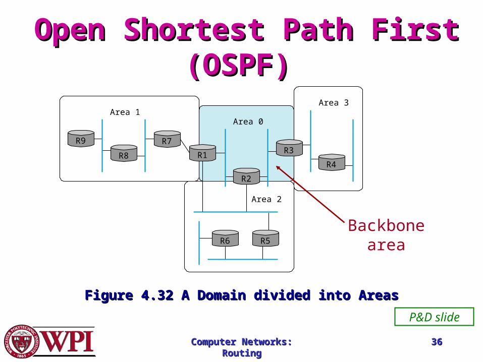
Open Shortest Path FirstOpen Shortest Path First(OSPF)(OSPF)
Area 1Area 0
Area 3
Area 2
R9
R8
R7
R1
R5R6
R4
R3
R2
Figure 4.32 A Domain divided into AreasFigure 4.32 A Domain divided into Areas
P&D slide
Backbonearea
Computer Networks: Computer Networks: RoutingRouting
3737
Open Shortest Path Open Shortest Path FirstFirst
(OSPF)(OSPF)• OSPF runs on top of IP, i.e., an OSPF packet is
transmitted with IP data packet header.• Uses Level 1 and Level 2 routers• Has: backbone routers, area border routers, and
AS boundary routers• LSPs referred to as LSAs (Link State
Advertisements)• Complex algorithm due to five distinct LSA
types.
Computer Networks: Computer Networks: RoutingRouting
3838
OSPF TerminologyOSPF Terminology
Internal router :: a level 1 router.
Backbone router :: a level 2 router.
Area border router (ABR) :: a backbone router that attaches to more than one area.
AS border router :: (an interdomain router), namely, a router that attaches to routers from other ASs across AS boundaries.
Computer Networks: Computer Networks: RoutingRouting
3939
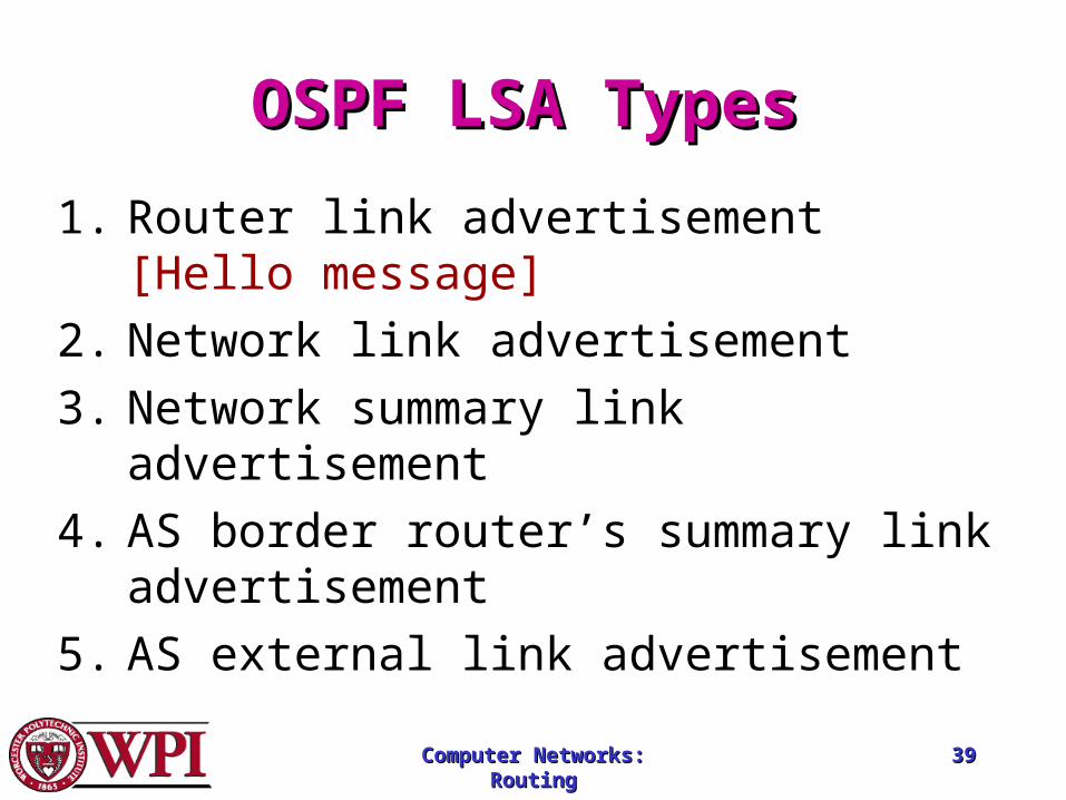
OSPF LSA TypesOSPF LSA Types
1. Router link advertisement [Hello message]
2. Network link advertisement
3. Network summary link advertisement
4. AS border router’s summary link advertisement
5. AS external link advertisement
Computer Networks: Computer Networks: RoutingRouting
4040
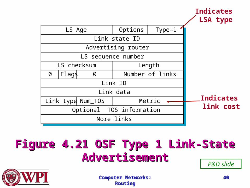
Figure 4.21 OSF Type 1 Link-State Figure 4.21 OSF Type 1 Link-State AdvertisementAdvertisement
LS Age Options Type=1
0 Flags 0 Number of links
Link type Num_TOS Metric
Link-state ID
Advertising router
LS sequence number
Link ID
Link data
Optional TOS information
More links
LS checksum Length
P&D slide
Indicates LSA type
Indicates link cost
Computer Networks: Computer Networks: RoutingRouting
4141
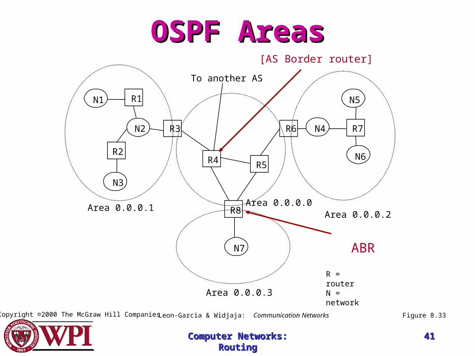
Area 0.0.0.1Area 0.0.0.2
Area 0.0.0.3
R1
R2
R3
R4 R5
R6 R7
R8
N1
N2
N3
N4
N5
N6
N7
To another AS
Area 0.0.0.0
R = router N = network
Figure 8.33Copyright ©2000 The McGraw Hill Companies Leon-Garcia & Widjaja: Communication Networks
OSPF AreasOSPF Areas[AS Border router]
ABR
Computer Networks: Computer Networks: RoutingRouting
4242
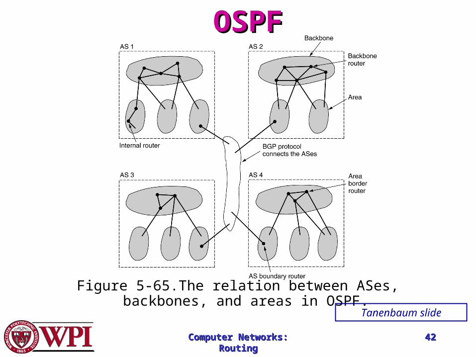
OSPFOSPF
Figure 5-65.The relation between ASes, backbones, and areas in OSPF.
Tanenbaum slide
Computer Networks: Computer Networks: RoutingRouting
4343
Border Gateway Border Gateway Protocol (BGP)Protocol (BGP)
• The replacement for EGP is BGP. Current version is BGP-4.
• BGP assumes the Internet is an arbitrary interconnected set of AS’s.
• In interdomain routing the goal is to find ANY path to the intended destination that is loop-free. The protocols are more concerned with reachability than optimality.
Recommended