Computational Study of the Hanbury Brown and Twiss Effect
Matthew Belzer
Laser Teaching Center
Department of Physics and Astronomy, Stony Brook University
Stony Brook, NY 11794
May 20, 2021
Abstract
In 1956, Robert Hanbury Brown and Richard Q. Twiss observed intensity correlations from visible
light that was produced by an incoherent source [1]. This experiment marked the birth of intensity
interferometry for visible wavelengths and in 1956 they applied their findings to measure the diameter of
the star Sirius [2]. Additionally, this experiment inspired the foundation of quantum optics and has been
used as evidence of photon bunching [3]. I have investigated their results by using Python to simulate the
emission of light with a randomized phase from two incoherent point sources. The light from each source
propagates to two detectors with a variable distance between them. I observed that the second order
correlation depended on the distance between the detectors sinusoidally, which was what we expected
from the analytic result. I generalized this two point simulation by simulating the intensity correlation
that comes from a star. My results matched what they found in their Sirius paper [2].
1

Contents
1 Introduction 3
1.1 Two Point Sources . . . . . . . . . . . . . . . . . . . . . . . . . . . . . . . . . . . . . . . . . . 5
1.2 NS Point Sources . . . . . . . . . . . . . . . . . . . . . . . . . . . . . . . . . . . . . . . . . . . 8
2 Computational Methods 11
2.1 Two Point Sources . . . . . . . . . . . . . . . . . . . . . . . . . . . . . . . . . . . . . . . . . . 11
2.2 NS Point Sources on a Star . . . . . . . . . . . . . . . . . . . . . . . . . . . . . . . . . . . . . 12
3 Results and Discussion 13
3.1 Two Point Sources . . . . . . . . . . . . . . . . . . . . . . . . . . . . . . . . . . . . . . . . . . 13
3.2 NS Point Sources on a Star . . . . . . . . . . . . . . . . . . . . . . . . . . . . . . . . . . . . . 14
3.2.1 Randomized Sources . . . . . . . . . . . . . . . . . . . . . . . . . . . . . . . . . . . . . 14
3.2.2 Equally Distributed Sources . . . . . . . . . . . . . . . . . . . . . . . . . . . . . . . . . 17
3.2.2.1 Phase Convergence Testing . . . . . . . . . . . . . . . . . . . . . . . . . . . . 20
3.2.3 Discussion . . . . . . . . . . . . . . . . . . . . . . . . . . . . . . . . . . . . . . . . . . . 26
4 Conclusion 28
5 Acknowledgements 28
2

1 Introduction
Light that travels in the#»
k direction has an electric field amplitude described by
E( #»r , t) = E0ei(
#»k · #»r−ωt+φ) (1)
where E0 is the amplitude of the wave,#»
k is the wave vector, #»r is a point in space, t is the time, ω is the
angular frequency, and φ is the phase. The irradiance of the light, I, is proportional to E( #»r , t) multiplied
with its complex conjugate
I( #»r , t) ∝ E( #»r , t)E∗( #»r , t) = E0ei(
#»k · #»r−ωt+φ)E0e
−i( #»k · #»r−ωt+φ) = E2
0 (2)
Typically, I is thought to be the intensity but this is incorrect [4]. In actuality, the intensity is the power
per unit solid angle per unit area, where a solid angle is the 3D equivalent to a two dimensional angle [4].
The irradiance on the other hand, is the power per unit area [4]. However, in the case of this paper, there
is no meaningful difference between the two because the constants that differentiate them cancel out when
the math is done.
The degree of spatial coherence between two point sources (1 and 2) can be calculated using the first
order correlation function
g(1) =〈E1( #»r1, t)E
∗2 ( #»r2, t)〉√
I1I2(3)
where E1 and E2 are the amplitudes at the first point ( #»r1) and the second point ( #»r2) and I1 and I2 are the
intensities at the first and second points respectively [4]. The angular brackets in the numerator denote a
time average. This is known as a first order correlation [4]. The denominator normalizes the numerator so
that the range of the correlation is [-1, 1]. If |g(1)| = 1 the light is completely coherent, but if |g(1)| = 0,
the light is completely incoherent. Otherwise, it is said that the light is partially coherent. The degree of
coherence of light can physically be measured using fringe visibility.
The second order correlation, which is also known as the intensity correlation, measures the correlation
between the intensities at two points [5].
g(2) =〈I1I2〉〈I1〉〈I2〉
(4)
Intensity correlations differ from first order correlations because their range is [0,2]. Additionally, the first
order correlation is impacted by phase, but the second order correlation is not since the phase of the light
cancels out when calculating the time averaged intensity at a point.
Hanbury Brown and Twiss (HBT) successfully measured the intensity correlation of visible light emitted
3
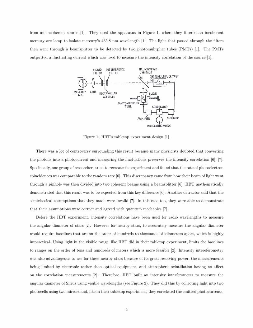
from an incoherent source [1]. They used the apparatus in Figure 1, where they filtered an incoherent
mercury arc lamp to isolate mercury’s 435.8 nm wavelength [1]. The light that passed through the filters
then went through a beamsplitter to be detected by two photomulitplier tubes (PMTs) [1]. The PMTs
outputted a fluctuating current which was used to measure the intensity correlation of the source [1].
Figure 1: HBT’s tabletop experiment design [1].
There was a lot of controversy surrounding this result because many physicists doubted that converting
the photons into a photocurrent and measuring the fluctuations preserves the intensity correlation [6], [7].
Specifically, one group of researchers tried to recreate the experiment and found that the rate of photoelectron
coincidences was comparable to the random rate [6]. This discrepancy came from how their beam of light went
through a pinhole was then divided into two coherent beams using a beamsplitter [6]. HBT mathematically
demonstrated that this result was to be expected from this key difference [6]. Another detractor said that the
semiclassical assumptions that they made were invalid [7]. In this case too, they were able to demonstrate
that their assumptions were correct and agreed with quantum mechanics [7].
Before the HBT experiment, intensity correlations have been used for radio wavelengths to measure
the angular diameter of stars [2]. However for nearby stars, to accurately measure the angular diameter
would require baselines that are on the order of hundreds to thousands of kilometers apart, which is highly
impractical. Using light in the visible range, like HBT did in their tabletop experiment, limits the baselines
to ranges on the order of tens and hundreds of meters which is more feasible [2]. Intensity intereferometry
was also advantageous to use for these nearby stars because of its great resolving power, the measurements
being limited by electronic rather than optical equipment, and atmospheric scintillation having no affect
on the correlation measurements [2]. Therefore, HBT built an intensity interferometer to measure the
angular diameter of Sirius using visible wavelengths (see Figure 2). They did this by collecting light into two
photocells using two mirrors and, like in their tabletop experiment, they correlated the emitted photocurrents.
4

Figure 2: HBT’s Sirius experimental design [2]
To determine the angular diameter θUD of the star, HBT assumed that the star is a uniform circular disk
and they derived the intensity correlation to be
g(2) = 1 +
[2J1(πθUDd/λ)
πθUDd/λ
]2(5)
where J1(x) is the first order Bessel Function and d is the distance between the detectors. Using this method,
they got a reasonable angular diameter of .0068” ± .0005”, which was close to the theoretical value of .0063”
[2].
1.1 Two Point Sources
There is an analytic solution for the intensity correlation between two incoherent point sources (A and
B) that emit light to two detectors (1 and 2) [5] (see Figure 3).
Figure 3: The two source, two detector condition.
The sources are separated by a distance D and the detectors are separated by a distance d. The sources
5

and detectors are separated by a distance L. The paths between each detector and each source are described
by lSource Detector. The light emitted from Source A has a phase of φa and an amplitude of a and the light
emitted from Source B has a phase of φb and an amplitude of b. Therefore, the amplitudes at Detectors 1
and 2 are described by
E1 = aei(klA1+φa) + bei(klB1+φb) (6)
E2 = aei(klA2+φa) + bei(klB2+φb) (7)
I have ignored the time terms in the amplitudes because they can essentially be included in the phase term
[5]. Using Eq. 2, the subsequent intensities are
I1 = a2 + b2 + abei(k(lA1−lB1)+φb−φa) + abe−i(k(lA1−lB1)+φb−φa) (8)
I2 = a2 + b2 + abei(k(lA2−lB2)+φb−φa) + abe−i(k(lA2−lB2)+φb−φa) (9)
Since there is a random phase difference in each of the exponential terms, when the intensities are individually
time averaged those terms go to zero. This happens because across a large enough time frame, the phases
will change infinitely many times since it is an incoherent source. This averaging yields
〈I1〉 = 〈I2〉 = a2 + b2 (10)
The product of the intensities is
I1I2 = (a2 + b2)2 + a3bei(k(lA1−lB1)+φb−φa) + a3be−i(k(lA1−lB1)+φb−φa) + ab3ei(k(lA1−lB1)+φb−φa)
+ ab3e−i(k(lA1−lB1)+φb−φa) + a3bei(k(lA2−lB2)+φb−φa) + a3be−i(k(lA2−lB2)+φb−φa) + ab3ei(k(lA2−lB2)+φb−φa)
+ ab3e−i(k(lA2−lB2)+φb−φa) + a2b2ei(k(lA1−lB1)+φb−φa+k(lA2−lB2)+φb−φa)
+ a2b2e−i(k(lA1−lB1)+φb−φa+k(lA2−lB2)+φb−φa)
+ a2b2ei(k(lA1−lB1−lA2+lB2)) + a2b2e−i(k(lA1−lB1−lA2+lB2)) (11)
The last two terms are the most important terms because the phases cancel out, leaving only constant terms.
When I time averaged the product of the intensities and used the identity eix + e−ix = 2 cos(x), I get
〈I1I2〉 = (a2 + b2)2 + a2b2ei(k(lA1−lB1−lA2+lB2)) + a2b2e−i(k(lA1−lB1−lA2+lB2))
= (a2 + b2)2 + 2a2b2 cos(k(lA1 − lB1 − lA2 + lB2)) (12)
6
Plugging these equations into Eq. 4, I get
g(2) =(a2 + b2)2 + 2a2b2 cos(k(lA1 − lB1 − lA2 + lB2))
(a2 + b2)2= 1 +
2a2b2 cos(k(lA1 − lB1 − lA2 + lB2))
(a2 + b2)2(13)
which shows that the path length that the light travels has a sinusoidal affect on the intensity correlation in
a two source, two detector system.
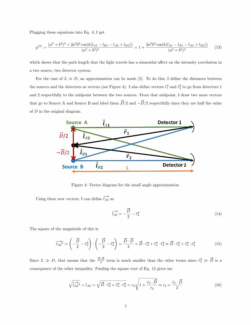
For the case of L � D, an approximation can be made [5]. To do this, I define the distances between
the sources and the detectors as vectors (see Figure 4). I also define vectors #»r1 and #»r2 to go from detectors 1
and 2 respectfully to the midpoint between the two sources. From that midpoint, I draw two more vectors
that go to Source A and Source B and label them#»
D/2 and − #»
D/2 respectfully since they are half the value
of D in the original diagram.
Figure 4: Vector diagram for the small angle approximation.
Using these new vectors, I can define# »
lA2 as
# »
lA2 = −#»
D
2− #»r2 (14)
The square of the magnitude of this is
# »
lA22 =
(−
#»
D
2− #»r2
)·
(−
#»
D
2− #»r2
)=
#»
D · #»
D
4+
#»
D · #»r2 + #»r2 · #»r2 ≈#»
D · #»r2 + #»r2 · #»r2 (15)
Since L � D, that means that the#»D· #»D4 term is much smaller than the other terms since #»r2 �
#»
D is a
consequence of the other inequality. Finding the square root of Eq. 15 gives me
√# »
lA22 = lA2 =
√#»
D · #»r2 + #»r2 · #»r2 = r2
√1 +
r̂2 ·#»
D
r2≈ r2 +
r̂2 ·#»
D
2(16)
7

The final equation comes from the approximation (1 +x)n ≈ 1 +nx and in this case n = .5. Using the same
process, equivalent values can be found for the rest of the path lengths.
lA1 ≈ r1 +r̂1 ·
#»
D
2(17)
lB1 ≈ r1 −r̂1 ·
#»
D
2(18)
lB2 ≈ r2 −r̂2 ·
#»
D
2(19)
Plugging these terms back into the cosine argument of Eq. 13 yields
k(lA1 − lB1 − lA2 + lB2) = k
(r1 +
r̂1 ·#»
D
2− r2 −
r̂2 ·#»
D
2− r1 +
r̂1 ·#»
D
2+ r2 −
r̂2 ·#»
D
2
)
= k(r̂1 ·#»
D − r̂2 ·#»
D) =#»
D · (r̂1 − r̂2)k =#»
D · ( #»
k1 −#»
k2) (20)
where#»
ki = k #»ri. Plugging this argument back into Eq. 13 gives me
g(2) = 1 +2a2b2 cos(
#»
D · (k̂1 − k̂2))
(a2 + b2)2(21)
An important note to make is that the oscillations of the cosine term will be most easily observed on a
detector separation of d = λ/θ where θ = R/L is the angular separation between the two points [5]. This
relationship recalls the Fraunhofer diffraction result in Eq. 5, since this equation is similar to the equation
for the radius of an Airy disk’s first dark ring [4]. Where Airy disks are the diffraction patterns that emerge
from circular apertures [4].
1.2 NS Point Sources
The intensity correlation for NS point sources can be thought of as the superposition of all of the intensity
correlations between all of the pairs of sources. To demonstrate this, I found the solution for the intensity
correlation of a three point source, two detector system. The light emitted from sources A, B, and C will
have amplitudes of a, b, and c respectively. The phases from sources A, B, and C will be φa, φb, and φc The
distance between the sources and detectors will be done using the same nomenclature as Section 1.1. The
amplitudes of detectors 1 and 2 are
8

E1 = aei(klA1+φa) + bei(klB1+φb) + cei(klC1+φc) (22)
E2 = aei(klA2+φa) + bei(klB2+φb) + cei(klC2+φc) (23)
The intensities are therefore
I1 = a2 + b2 + c2 + abei(k(lA1−lB1)+φb−φa) + abe−i(k(lA1−lB1)+φb−φa)
+ acei(k(lA1−lC1)+φc−φa) + ace−i(k(lA1−lC1)+φb−φa)
+ bcei(k(lB1−lC1)+φc−φb) + bce−i(k(lB1−lC1)+φb−φc) (24)
I2 = a2 + b2 + c2 + abei(k(lA2−lB2)+φb−φa) + abe−i(k(lA2−lB2)+φb−φa)
+ acei(k(lA2−lC2)+φc−φa) + ace−i(k(lA2−lC2)+φb−φa)
+ bcei(k(lB2−lC2)+φc−φb) + bce−i(k(lB2−lC2)+φb−φc) (25)
The time averages of the intensities are just the constants since the exponentials have a random phase
〈I1〉 = 〈I2〉 = a2 + b2 + c2 (26)
This is very similar to Eq. 10, except there is an additional amplitude square. So, this can be generalized
for n points to just being the sum of the squares of the amplitude coefficients.
I used Mathematica to find the product of the intensities in Eq. 24 and 25 since there are 92 terms
(see Figure 5). The naming convention is slightly different for my Mathematica results. The amplitudes are
labelled the same, but their respective phases are pa, pb, and pc, not φ. I also dropped the l and made the
subscript the distances between the sources and detectors, so the distance between Source B and Detector 1
is B1 instead of lB1.
9

Figure 5: The three source and two detector system I1 × I2 expansion.
The term underlined in black is all of the constants and can be rewritten as (a2 + b2 + c2)2. Due to the
identity of eix+e−ix = 2 cos(x), the terms underlined in green can be rewritten as 2a2b2 cos(k(lA1−lB1−lA2+
lB2)). Similarly, the terms underlined in red and purple can be rewritten as 2a2c2 cos(k(lA1−lC1−lA2+lC2)).
and 2b2c2 cos(k(lB1 − lC1 − lB2 + lC2)) respectively. These terms are important because their phases cancel
out and the rest of the terms go to zero when the time average is done. Hence,
〈I1I2〉 = (a2 + b2 + c2)2 + 2a2b2 cos(k(lA1 − lB1 − lA2 + lB2)) + 2a2c2 cos(k(lA1 − lC1 − lA2 + lC2))
+ 2b2c2 cos(k(lB1 − lC1 − lB2 + lC2)) (27)
Therefore, the resulting second order correlation is in the form of
g(2) =(a2 + b2 + c2)2 + 2a2b2 cos(k(lA1 − lB1 − lA2 + lB2)) + 2a2c2 cos(k(lA1 − lC1 − lA2 + lC2))
(a2 + b2 + c2)2
+2b2c2 cos(k(lB1 − lC1 − lB2 + lC2))
(a2 + b2 + c2)2= 1 + 2
a2b2 cos(k(lA1 − lB1 − lA2 + lB2))
(a2 + b2 + c2)2
+ 2a2c2 cos(k(lA1 − lC1 − lA2 + lC2)) + b2c2 cos(k(lB1 − lC1 − lB2 + lC2))
(a2 + b2 + c2)2(28)
10

For the case of NS sources, this can be generalized to
g(2) = 1 + 2a2b2 cos(k(lA1 − lB1 − lA2 + lB2)) + a2c2 cos(k(lA1 − lC1 − lA2 + lC2))
(a2 + b2 + c2 + ...)2
+ 2b2c2 cos(k(lB1 − lC1 − lB2 + lC2)) + ...
(a2 + b2 + c2 + ...)2(29)
where the numerator of the fraction is all of the combinations of path differences and source amplitudes
using that sign convention and the denominator is the sum of the squares of all the source amplitudes. It is
important to note that there should be C(NS , 2) cosine terms in the numerator since the cosine terms are
combinations of sources. To show that this is true, for two sources, there is one cosine term and C(2,2) = 1
and for three sources, there are three cosine terms and C(3,2) = 3.
2 Computational Methods
The full simulation code can be viewed on GitHub:
https://github.com/MatthewBelzer/HBT-Simulations.
2.1 Two Point Sources
To simulate the intensity correlations, I considered light with randomly generated phases differences from
two sources Np times and found the intensity correlation for each iteration and averaged it. This was done
for Nd discrete distances between 0 and d. A more detailed explanation of the code can be found below
1. Give values to the following constants: the wave number k, the positions of the sources, the number
of random phases Np, the number of detector distances Nd, and the range of the detector distances.
2. For the Nd distances in the distance array:
(a) Calculate the distances between the sources and the detectors.
(b) Find the theoretical value using Eq. 13
(c) For Np phase differences in the randomly generated phase array:
i. Use Eq. 1 and 2 to find the amplitudes and the intensities at each of the detectors.
ii. Correlate these intensities using Eq. 4.
(d) Average the correlations across all of the phases.
For the simulation, k was set to 108 rad/m, there were 100 distances calculated (Nd), and there were
1000 random phase differences between 0 and 2π (Np). The amplitudes for both sources were set to 1. The
11
positions of Source A and Source B were (0, 100) m and (0, -100) m respectively. The positions of detectors
1 and 2 were (106, d/2) m and (106, −d/2) m respectively, where d ranged between 0 and 1 mm.
2.2 NS Point Sources on a Star
To verify HBT’s Sirius results, I generated NS points on the surface of a hemisphere facing the detectors
so that all of those sources appear like a star. The rest of the simulation was the practically the same as
the two point simulation except that I generalized the distances and the random phases using arrays. A
description of my code can be found below
1. Give values to the following constants: the wave number k, the number of random phases Np, the
number of detector distances Nd, the range of the detector distances, number of sources NS , y distance
from the midpoint of the detectors to the surface of the star, and star radius R.
2. Generate NS points on the surface of a star facing my detector positions
3. For the Nd distances in the distance array:
(a) For NS Sources:
i. Calculate the distance from each source to each detector
(b) Find the theoretical value using Eq. 29
(c) For Np phases:
i. Generate a phase array that has a phase for each of the NS sources
ii. Use Eq. 1 and 2 to find the amplitudes and the intensities at each of the detectors.
iii. Correlate these intensities using Eq. 4.
(d) Average the correlations across all of the phases.
I generated sources on the surface of the star using two methods. The first method was randomized and
the second method used an algorithm that generated a Fibonacci Sphere, which makes the points roughly
equidistant form each other [8].
An important part of my code that I want to highlight is my method of calculating the theoretical curve.
I used a recursive method where I found the cosine numerator terms between the first source and all other
sources. Next I removed the first source from my distance arrays and found the cosine terms for the second
source and all other sources. I then removed the second source from my distance arrays and found the cosine
terms for the third source and all other sources. I repeated this until I had one source left in the array. This
method lets me find the theoretical curve for any number of NS sources.
12

For my first simulations, k was set to 108 rad/m, there were 100 distances calculated (Nd), and there
were 2000 random phase differences between 0 and 2π (Np). The amplitudes for all of the sources were set
to 1. I generated 1000 sources on the surface of a hemisphere of Radius 100m that’s center was 1000 km
away from the midpoint of the detectors. The positions of detectors 1 and 2 were (0, d/2) m and (0, −d/2)
respectively, where d ranged between 0 and 1 mm. It is important to note that this simulation is not a
realistic star, but I chose these values since they were within the same orders of magnitude as the two source
experiment.
To test the convergence of the phases, I reduced the number of distances calculated to 20 and I had those
distance points range from 0 to .5 mm. I generated 3000 source points using the Fibonacci method and I
set three different values for Np: 100, 5000, and 10000 random phases.
3 Results and Discussion
3.1 Two Point Sources
Using the conditions that I described in Section 2.1, I graphed the intensity correlation in Figure 6. The
simulated data points are a very good fit for the theoretical curve because χ299 = .018655 (where there are 99
degrees of freedom) and p ≈ 1. A p-value being equal to one shows that it is a very strong fit. Additionally,
since a and b both equal 1, the coefficient in front of the cosine term is 1/2 and the data points do go 1/2
above and below 1.
Figure 6: Two source simulation.
13
3.2 NS Point Sources on a Star
3.2.1 Randomized Sources
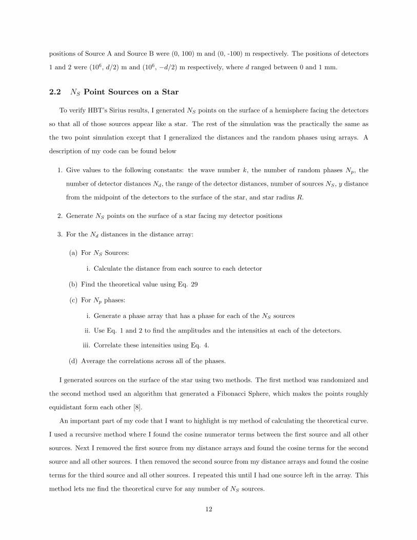
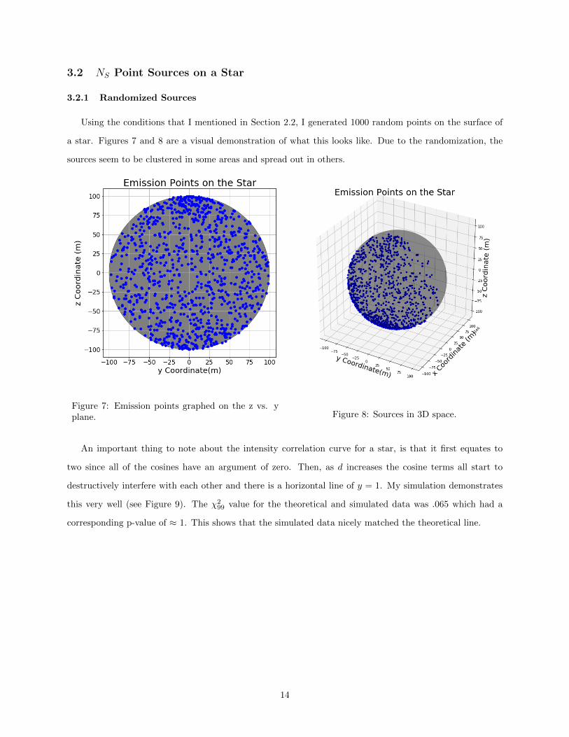
Using the conditions that I mentioned in Section 2.2, I generated 1000 random points on the surface of
a star. Figures 7 and 8 are a visual demonstration of what this looks like. Due to the randomization, the
sources seem to be clustered in some areas and spread out in others.
Figure 7: Emission points graphed on the z vs. yplane. Figure 8: Sources in 3D space.
An important thing to note about the intensity correlation curve for a star, is that it first equates to
two since all of the cosines have an argument of zero. Then, as d increases the cosine terms all start to
destructively interfere with each other and there is a horizontal line of y = 1. My simulation demonstrates
this very well (see Figure 9). The χ299 value for the theoretical and simulated data was .065 which had a
corresponding p-value of ≈ 1. This shows that the simulated data nicely matched the theoretical line.
14

Figure 9: NS source simulation plotted against theoretical curve.
The angular diameter of my simulated sphere is 2 tan(100/106) = 200 µrads. Using Eq. 5, I fitted my
simulated data to extract the angular diameter (see Figure 10). I got a value of 188.3 ± 1.7 µrads, which
has a small relative error of 5.85%. The fit looks quite good, but it is still slightly off. The residual of the
plot looks quite good since its slope is quite small and there is a small intercept (see Figure 11). Therefore,
I think the fit is good.
Figure 10: Fitted NS source simulation for 1000 random sources.
15

Figure 11: NS source simulation for 1000 random sources residual.
I also fitted the theoretical values that I calculated using Eq. 29 (see Figure 12). I got a value of 184.32
± .37 µrads, which is surprisingly smaller than what I found using the randomized phases. This value has
a relative error of 7.84%. I also graphed the residual and the data seemed to oscillate around the x-axis to
varying degrees (see Figure 13). Hence, I am doubtful of the quality of this fit.
Figure 12: Fitted NS source theory for 1000 random sources.
16

Figure 13: NS source theory for 1000 random sources residual.
3.2.2 Equally Distributed Sources
Using the conditions that I established in Section 2.2, I generated 1000 roughly equidistant points on the
surface of a star using a modified version of the Fibonacci sphere algorithm. Figures 14 and 15 are a visual
demonstration of this technique. Notably, this method avoids the clustering problems present in randomized
source generation.
Figure 14: Emission points graphed on the z vs. yplane using the Fibonacci method. Figure 15: Sources in 3D space Fibonacci algorithm.
This simulation had a χ299 value of .051 which has a p-value of ≈ 1 (see Figure 16). Therefore, the
theoretical curve is a very good fit for the simulated data points. It appears that the second maxima is
17

larger for this graph when compared to the randomized source simulation.
Figure 16: 1000 Fibonacci sources simulation plotted against theoretical curve.
As I did in the previous section, I fitted my simulated data to find the angular diameter (see Figure
17). I got a value of 233.5 ± 2.1 µrads, which has a relative error of 16.75%. The residual of the plot looks
reasonable, but there is still a prominent upward trend in the data (see Figure 18). That being said, the fit
seems decent.
Figure 17: Fitted NS source simulation for 1000 equidistant sources.
18
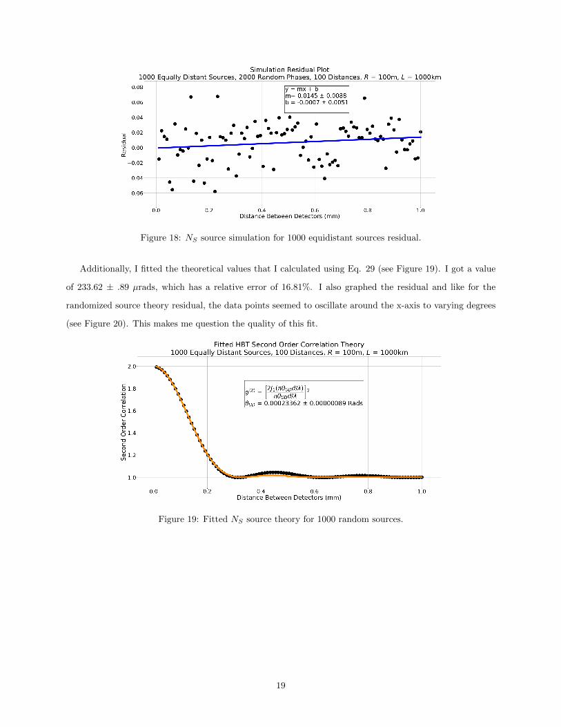
Figure 18: NS source simulation for 1000 equidistant sources residual.
Additionally, I fitted the theoretical values that I calculated using Eq. 29 (see Figure 19). I got a value
of 233.62 ± .89 µrads, which has a relative error of 16.81%. I also graphed the residual and like for the
randomized source theory residual, the data points seemed to oscillate around the x-axis to varying degrees
(see Figure 20). This makes me question the quality of this fit.
Figure 19: Fitted NS source theory for 1000 random sources.
19

Figure 20: NS source theory for 1000 random sources residual.
3.2.2.1 Phase Convergence Testing I have also tested if increasing the number of phases causes the
data points to converge to the theoretical value. To do this, I increased the number of points I sampled
from 1000 to 3000 (see Figure 21 & 22). I also used the Fibonacci sampling method because it would keep
the points constant, which eliminates a source of error. To save on computational time, I calculated the
correlations for 20 distances instead of 100 and I also halved the range of my data from [0, 1] mm to [0, .5]
mm. Using these conditions, I found the correlations for three phase values: 100, 5000, and 10000.
Figure 21: 3000 emission points graphed on the zvs. y plane using the Fibonacci method. Figure 22: 3000 sources in 3D space using the Fi-
bonacci method.
Figure 23, which used 100 phases, has a χ219 value of .28 and a p-value of ≈ 1. Despite this, the theoretical
20

values still match up decently with the simulated data.
Figure 23: Simulation of 3000 evenly spaced sources and 100 phases.
Since the theoretical fit will be the same for all the variations of the phase, I only need to find the angular
diameter using the theoretical fit once. I got an angular diameter of 233.7 ± 1.9 µrads, which has a relative
error of 16.85% (see Figure 24). The residual has a significant slope and the data points are oscillating
around the x-axis (see Figure 25). This leads me to doubt the quality of the fit.
Figure 24: Fitted NS source theory for 3000 random sources.
21

Figure 25: NS source theory for 3000 random sources residual.
The fit for the simulated data points gave me an angular diameter of 250 ± 18 µrads which has a large
relative error of 25% when compared to the expected value (see Figure 26). The residual has a significant
upward trend and the magnitudes of the residuals are much larger than I have seen in previous simulations,
which is why the absolute error of the angular diameter is an order of magnitude larger than I have previously
observed (see Figure 27).
Figure 26: Fitted NS source simulation for 3000 equidistant sources and 100 phases.
22

Figure 27: Residual for the simulation with 3000 equidistant sources and 100 phases.
The simulation with 5000 phases has a χ219 value of .004670 with a p-value that is ≈ 1 (see Figure 28).
As such, the theoretical curve is a good fit.
Figure 28: Simulation of 3000 evenly spaced sources and 5000 phases.
Fitting the simulated data points gave me an angular diameter of 236.4 ± 2.8 µrads (see Figure 29). This
has a relative error of 18.2%. The residual of the data has a linear slope, but this slope is smaller than the
100 phase fit’s slope, suggesting that this fit is better (see Figure 30).
23

Figure 29: Fitted NS source simulation for 3000 equidistant sources and 5000 phases.
Figure 30: Residual for the simulation with 3000 equidistant sources and 5000 phases.
Lastly, the 10,000 phase simulation yielded a χ219 value of .00468 with a p-value that is ≈ 1, which means
that the theoretical curve is a good fit (see Figure 31).
24

Figure 31: Simulation of 3000 evenly spaced sources and 5000 phases.
Fitting the simulated data points for this condition gave me an angular diameter of 231.2 ± 2.5 µrads
(see Figure 32). This has a relative error of 15.6%. The residual of the data has a linear slope, but this slope
is smaller than the 5000 phase fit’s slope, meaning that this fit is better (see Figure 33).
Figure 32: Fitted NS source simulation for 3000 equidistant sources and 10000 phases.
25

Figure 33: Residual for the simulation with 3000 equidistant sources and 10000 phases.
3.2.3 Discussion
A summary of my results for the different sources can be found in Table 1 and Table 3. A summary
of the relative errors for the different sources can be found in Table 2 and Table 4. A summary of the fit
statistics for the 3000 Fibonacci sources can be found in Table 5.
Summary of the NS=1000 Sources ResultsData Randomized Sources Equidistant SourcesType Angular Diameter (µrads) Angular Diameter (µrads)
Simulation 188.3 ± 1.7 233.5 ± 2.1Theory 184.32 ± .37 233.62 ± .89
Table 1: The summary of my 1000 sources results.
Summary of the NS = 1000 Sources Relative ErrorsType Randomized Sources Relative Error Equidistant Sources Relative Error
Simulation 5.85% 16.75%Theory 7.84% 16.81%
Table 2: The summary of my 1000 sources relative errors.
Summary of the NS = 3000 Equidistant Sources ResultsType Angular Diameter (µrads)
Theory 233.7 ± 1.9Np = 100 250 ± 18Np = 5000 236.4 ± 2.8Np = 10000 231.2 ± 2.5
Table 3: The summary of my 3000 equidistant sources results.
26

Summary of the NS = 3000 Equidistant Sources Relative ErrorsType Relative Error
Theory 16.85%Np = 100 25%Np = 5000 18.2%Np = 10000 15.6%
Table 4: The summary of my 3000 equidistant sources relative errors.
Summary of the Statistics for the NS = 3000 Equidistant SourcesNumber of Phases χ2
19 p-value100 .28 ≈ 15000 0.00470 ≈ 110000 0.00468 ≈ 1
Table 5: The summary of my 3000 equidistant sources statistics.
My results in Tables 1 & 2 are the opposite of what I would expect. I would think that the theoretical fits
would be closer to the actual value of 200 µrads and that the equidistant sources would be closer to the actual
value than the randomized sources. It also interesting that the randomized sources produce a value that is
below the expected value and the equidistant sources produce a value that is above the expected result. I
think this is just because of the specific point configuration that was generated and there are probably just
as many randomized source configurations that would yield a result larger than the expected result.
The results in Tables 3 & 4 shows that as the number of phases increases, the measured angular diameter
is closer to the actual value. Interestingly, the angular data that corresponds to the 10,000 phases has a
smaller relative error than the theoretical curve. I think this may just be the randomness of the phases
assisting the measurement and that there are probably other random configurations of phase that would
negatively impact the relative error. Additionally, since the χ219 values in Table 5 are decreasing as the phase
count is increasing, I can conclude that an infinite number of phases would converge to the theoretical value.
However, since the p-values are all roughly the same there aren’t any major significant differences between
the three phases.
Another interesting observation is that the 3000 equidistant source star’s fitted theoretical angular di-
ameter has a slightly larger relative error than the 1000 equidistant source star’s fitted theoretical angular
diameter. I am unsure as to why this is, although there are a variety of possible reasons that all the angular
diameters do not match the expected result more closely. For example, the approximation that the star is a
circular disk could be causing a significant error. Similarly, my method of representing a star by placing NS
point sources on the surface of a hemisphere may not be entirely accurate. Another possible error is that I
did not use enough source points in the simulation because stars are made up of many more atoms, which
function as point emitters, than I could possibly simulate. Lastly, since I concluded that an infinite number
27

of phases converges to the theoretical value, a small sample of random phases cannot be a source of error
since the theoretical values are still off.
4 Conclusion
The Hanbury Brown and Twiss experiments demonstrated the possibility and applicability of intensity
correlations in the visible spectrum using PMTs. I have successfully derived the intensity correlation formulas
for two and three source systems and I have further generalized those results for a system of NS sources. I first
tested these formulas by simulating the intensity correlations for a two source system where the simulated
data points statistically matched the theoretical curve. I simulated the generalized formula by choosing
data points on the surface of a star using two methods: randomly and using the Fibonacci Algorithm.
Surprisingly, the random method proved to be more accurate, but I think that this is just because of the
specific configuration of source points that was randomly chosen. Some other possible errors could be that
the assumption that the star is a circular disk is not good, not sampling enough sources, and my model of
the star may be inaccurate. I have also shown that increasing the number of randomized phases results in a
decreased χ219 which means that an infinite number of phases would likely converge to the theoretical curve.
5 Acknowledgements
I’d like to make a special note that Abhishek Cherath and I worked together on the two point source
simulation. I’d also like to thank Dr. Eric Jones, Dr. Marty Cohen, and Professor Harold Metcalf for their
help and guidance in this project.
28

References
[1] Hanbury Brown, R., & Twiss, R. Q. “Correlation between Photons in two Coherent Beams of Light”.
In: Nature 177.4497 (1956), pp. 27–29. doi: https://doi.org/10.1038/177027a0.
[2] Hanbury Brown, R., & Twiss, R. Q. “A Test of a New Type of Stellar Interferometer on Sirius.” In:
Nature 178.4497 (1956), pp. 1046–1048. doi: https://doi.org/10.1038/1781046a0.
[3] Hanbury Brown, R., & Twiss, R. Q. “Interferometry of the intensity fluctuations in light - I. Basic
theory: the correlation between photons in coherent beams of radiation”. In: Royal Publishing Society
242 (1957), pp. 300–324. doi: https://doi.org/10.1098/rspa.1957.0177.
[4] Grant R. Fowles. Introduction to Modern Optics. 2nd ed. New York, USA: Dover Publications, inc.,
1989.
[5] Gordon, B. “The physics of Hanbury Brown–Twiss intensity interferometry: from stars to nuclear col-
lisions”. In: Acta Physica Polonica B 29 (1998), pp. 1839–1884. url: https://arxiv.org/abs/nucl-
th/9804026v2.
[6] R. Hanbury Brown and R. Q. Twiss. “The Question of Correlation between Photons in Coherent Light
Rays”. In: Nature 178.4548 (Dec. 1, 1956), pp. 1447–1448. issn: 1476-4687. doi: 10.1038/1781447a0.
url: https://doi.org/10.1038/1781447a0.
[7] Hanbury Brown, R., & Twiss, R. Q. “The Question of Correlation between Photons in Coherent Beams
of Light”. In: Nature 179.4570 (1957), pp. 1128–1129. doi: https://doi.org/10.1038/1791128a0.
[8] Evenly distributing n points on a sphere. url: https://stackoverflow.com/questions/9600801/
evenly-distributing-n-points-on-a-sphere.
29
Recommended