29th
Symposium on Naval Hydrodynamics
Gothenburg, Sweden, 26-31 August 2012
1 Current affiliation: Center for Advanced Vehicular Systems, Mississippi State University, Starkville, MS 39759
2 Current affiliation: Mechanical Engineering Department, University of Idaho, Moscow, ID 83844
Computational Ship Hydrodynamics: Nowadays and Way
Forward
Frederick Stern, Jianming Yang, Zhaoyuan Wang,
Hamid Sadat-Hosseini, Maysam Mousaviraad, Shanti Bhushan1, Tao Xing
2
(IIHR-Hydroscience & Engineering, University of Iowa,
Iowa City, IA 52242, USA)
ABSTRACT
Computational fluid dynamics for ship hydrodynamics
has made monumental progress over the last ten years,
which is reaching the milestone of providing first-
generation simulation-based design tools with vast
capabilities for model- and full-scale simulations and
optimization. This is due to the enabling technologies
such as free surface tracking/capturing, turbulence
modeling, 6DOF motion prediction, dynamic overset
grids, local/adaptive grid refinement, high performance
computing, environmental modeling, and optimization
methods. Herein, various modeling, numerical
methods, and high performance computing approaches
for computational ship hydrodynamics are evaluated
thereby providing a vision for the development of the
next-generation high-fidelity simulation tools. Verifica-
tion and validation procedures and their applications,
including resistance and propulsion, seakeeping,
maneuvering, and stability and capsize, are reviewed.
Issues, opportunities, and challenges for advancements
in higher-fidelity two-phase flow are addressed.
Fundamental studies for two-phase flows are also
discussed. Conclusions and future directions are also
provided.
1 INTRODUCTION
In just over 30 years computational fluid dynamics
(CFD) for ship hydrodynamics has surpassed all
expectations in reaching astronomical progress,
capabilities and milestone of providing the first-
generation simulation-based design (SBD) tools for
model- and full-scale simulations and optimization
enabling innovative cost-saving designs to meet the
challenges of the 21st century, especially with regard to
safety, energy and economy. CFD is changing the face
of ship hydrodynamics as the SBD approach is
replacing the now old-fashioned build-and-test
approach such that model testing is only required at the
final design stage; however, towing tank and wave
basin facilities are needed additionally for model
development and CFD validation, which requires even
more advanced measurement systems for global and
local flow variables and more stringent requirements
on experimental uncertainty analysis as it plays an
important role in validation procedures.
In the following, the development of computa-
tional ship hydrodynamics over the past 30 years is
briefed using example references idiosyncratic to the
authors and their colleagues. In the early 1980s integral
methods still predominated, which worked well for
two-dimensions but had great difficulty in extensions
to three-dimensions due to inability to model cross-
flow velocity profiles (von Kerczek et al., 1984). Thus
three-dimensional boundary layer finite difference
methods were soon developed, which worked well for
thin boundary layers but had great difficulty for thick
boundary layers and flow separation (Stern, 1986).
Quickly partially parabolic approaches were developed
(Stern et al., 1988a) followed by full RANS solvers
with viscous-inviscid interaction approaches for
nonzero Froude number (Tahara et al., 1992). Soon
thereafter large domain RANS methods using free
surface tracking methods (Tahara et al., 1996) along
with extensions for improved turbulence and propulsor
modeling, multi-block, overset grids and parallel
computing were developed (Paterson et al., 2003)
allowing full/appended/model captive simulations for
resistance and propulsion. Next enabling technologies
of level-set free surface capturing, inertial reference
frames, and dynamic overset grids allowed wave
breaking and ship motions (Carrica et al. 2007) and of
anisotropic URANS and DES turbulence modeling
allowed better resolved turbulence (Xing et al., 2007;
2012). Extensions soon followed for semi-coupled air-
water flows (Huang et al., 2008), 6DOF simulations
using controllers for calm-water maneuvering (Carrica
et al., 2012b) and capsize predictions (Sadat-Hosseini
et al., 2011b) including rotating propellers (Carrica et
al., 2012a), exhaust plumes (Huang et al., 2012), wall
functions for full-scale DES simulations (Bhushan et
al., 2012c), damaged stability including motions
29th
Symposium on Naval Hydrodynamics
Gothenburg, Sweden, 26-31 August 2012
(Sadat-Hosseini et al., 2012c), and high performance
computing (HPC) (Bhushan et al., 2011a). Innovative
procedures not possible in towing tanks were also
developed for both resistance and propulsion (Xing et
al., 2008) and seakeeping (Mousaviraad et al., 2010)
and CFD with system identification has shown ability
for improvement in system-based mathematical models
for maneuvering in calm water and waves (Araki et al.,
2012a, b).
The next-generation high-fidelity SBD tools
are already under development for milestone achieve-
ment in increased capability focusing on orders of
magnitude improvements in accuracy, robustness, and
exascale HPC capability for fully resolved, fully
coupled, sharp-interface, multi-scale, multi-phase,
turbulent ship flow utilizing billions of grid points.
Current capabilities are for Cartesian grids with
immersed boundary methods (Yang and Stern, 2009;
Wang et al., 2009a, b), for orthogonal curvilinear grids
(Wang et al., 2012a, b), for overset Carte-
sian/orthogonal curvilinear grids (Bhushan et al.,
2011b), and extensions in progress for non-orthogonal
curvilinear grids. High-fidelity large eddy simulation
(LES) simulations for plunging breaking waves and
surface-piercing wedges and cylinders have resolved
for the first time and identified physics of the plunging
wave breaking process (Koo et al., 2012), spray
formation (Wang et al., 2010b) and wake spreading
(Suh et al., 2011). Realization non-orthogonal curvilin-
ear grids (Yang et al., 2012) will enable similarly
resolved simulations for practical geometries and
conditions with increased physical understanding
thereby revolutionizing ship design; however, consid-
erable research is still needed, as high-fidelity general
purpose solvers with the aforementioned functionality
do not yet exist.
Quantitative verification and validation
(V&V) procedures and an adequate number of well-
trained expert users are also essential ingredients for
the successful implementation of SBD. Here again,
computational ship hydrodynamics has played
leadership role in V&V (Stern et al., 2006a; Xing and
Stern, 2010) and development of CFD educational
interface for teaching expert users at both introductory
and intermediate levels (Stern et al., 2006b; 2012).
V&V research is still needed especially for single-grid
methods and LES turbulence models. General-purpose
CFD educational interfaces for teaching CFD are not
yet available.
The research paradigm of integrated code de-
velopment, experiments, and uncertainty analysis along
with step-by-step building block approach and
international collaborations for synergistic research
magnifying individual institute capabilities as exempli-
fied by IIHR (Stern et al., 2003) has been foundational
in the unprecedented achievements of computational
ship hydrodynamics.
Progress in CFD for ship hydrodynamics has
been well benchmarked in CFD workshops for
resistance and propulsion and seakeeping (most
recently, Larsson et al., 2011) and calm water maneu-
vering (Stern et al., 2011a) along with the Proceedings
of the ITTC both for applications and CFD itself.
Optimization capabilities for ship hydrodynamics were
recently reviewed by Campana et al. (2009). Sanada et
al. (2012) provides an overview of the past captive
towing tank and current free running wave basin
experimental ship hydrodynamics for CFD validation
as background for description of the new IIHR wave
basin and trajectories and local flow field measure-
ments around the ONR tumblehome in maneuvering
motion in calm water and head and following waves.
Computational ship hydrodynamics current
functionality, initiation of the development of the next
generation high-fidelity SBD tools, contributions to
V&V and CFD education, research paradigm and
international collaborations, CFD workshops and ITTC
Proceedings and optimization capabilities as demon-
strated by the example references given above arguably
equals if not surpasses other external flow industrial
applications such as aerospace, automotive and rolling
stock capabilities such that ship hydrodynamics in spite
of its relatively small size community is at the forefront
in computational science and technology and research
and development.
Herein computational ship hydrodynamics is
reviewed with a different perspective and special focus
on the critical assessment of modeling, numerical
methods and HPC both nowadays and prognosis for
way forward. Quantitative V&V procedures and their
application for evaluation of captive and free running
simulation capabilities along with fundamental studies
for two-phase flows are also reviewed with the latest
results obtained at IIHR as selected examples. Conclu-
sions and future directions are also provided.
2 COMPUTATIONAL SHIP HYDRODYNAM-
ICS
Application areas are at the core of computational
method requirements as they guide the choice of
modeling, which in return guide the grid and accuracy
requirements of the simulation. The grid requirements
along with HPC determine the efforts required for grid
generation, problem setup, solution turnaround time
and post processing efforts. Computational methods for
ship hydrodynamics include modeling, numerical
methods and HPC capability as summarized in Fig. 1.
Models required for naval applications are hydrody-
namics, air flow and two-phase flow solvers, turbu-
lence models, interface models, motion solvers,
29th
Symposium on Naval Hydrodynamics
Gothenburg, Sweden, 26-31 August 2012
propulsion models, sea condition or wave models, etc.
The numerical methods encompass the grids and
discretization schemes for the governing equations.
High performance computing encompasses the ability
to use larger grids, more parallel processors and
speedup solution turnaround time.
ITTC 2011 Specialist Committee on Compu-
tational Fluid dynamics report (ITTC, 2011) provides a
detailed review of numerical methods commonly used
for ship hydrodynamics. Most of them are also
discussed here, and readers are referred to ITTC (2011)
for the complete picture of CFD in ship hydrodynamics
from a different angle. The discussions herein focus on
the advantages and limitations of the computational
methods currently used in ship hydrodynamics, and
recommendation are made for the most appropriate
methods for a given application area. The following
two sections also review upcoming computational
methods focusing on the multiscale issues, which may
provide hints of new development directions of high
fidelity solvers for ship hydrodynamics. The upcoming
numerical methods include higher-order discretization
schemes and novel interface tracking schemes, and
HPC challenges of exascale computing.
3 MATHEMATICAL MODELING
3.1 Ship flows
The fluids involved in ship hydrodynamics are water
and air (vapor phase in cavitation can be treated as a
gas phase as the air in the solvers). In general, they can
be considered as Newtonian fluids. The flow phenom-
ena can also be considered as incompressible due to
usually very low Mach numbers. Therefore, the
governing equations for ship flows are the incompress-
ible Navier-Stokes equations. Solvers for ship flows
are categorized based on the solution methods for the
two different fluids involved in as: (a) free-surface
flow; (b) air flow; and (c) two-phase flow solvers.
3.1.1 Free-surface hydrodynamics
In free-surface flow solvers, only the water phase is
solved using atmospheric pressure boundary condition
at the free-surface. Many ship hydrodynamics solvers
have adopted mathematical models for free-surface
models, for example, CFDShip-Iowa versions 3
(Tahara et al., 1996) and 4 (Carrica et al., 2007) from
IIHR, ship (Di Mascio et al., 2007) from INSEAN,
SURF (Hino et al., 2010) from NMRI, PARNASSOS
(Hoekstra, 1999) from MARIN, ICARE (Ferrant et al.,
2008) from ECN/HOE, WISDAM (Orihara & Miyata,
2003) from the University of Tokyo, among others.
These solvers are applicable in a wide range of
applications, since the water phase accounts for most
resistance. However, most of these solvers are not
capable of solving problems with wave breaking and
air entrainment, which have become more and more
important in ship hydrodynamics due to the develop-
ment of non-conventional hull shapes and studies of
bubbly wake, among others.
3.1.2 Air Flows
For many problems in ship hydrodynamics, the effects
of air flow on the water flow are negligible but the air
flow around the ship is still of interest. This includes
analysis of environmental conditions and air wakes
around a ship in motion with complex superstructures,
maneuverability and seakeeping under strong winds,
capsizing, exhaust plumes (Huang et al., 2012a), etc.
Most CFD research of ship aero-hydrodynamics
simplified the problem by neglecting the free surface
deformation and velocities, which restricted the range
of problems that could be considered. A semi-coupled
approach was developed by Huang et al. (2008) where
the water flow is solved first and the air flow is solved
with the unsteady free-surface water flow as boundary
conditions. The limitation of the semi-coupled
approach is its inabilities to deal with air entrainment,
wind-driven wave generation, cavitation, etc., as the
water flow is only affected by the air flow through ship
motion driven by air flow load.
3.1.3 Two-phase flows
In the two-phase solvers, both the air and water phase
are solved in a coupled manner, which requires
treatment of the density and viscosity jump at the
interface (Huang et al., 2007; Yang et al., 2009). The
two-phase solvers are more common in commercial
codes such as FLUENT, CFX, STAR-CCM+
(COMET) and open-source CFD solver OpenFOAM,
as they are more general tools for a wide range of
applications. However, air flows including air entrain-
ment were seldom shown in ship flow applications
performed with these solvers, due to high total grid
resolution requirements for resolving the air flow
besides the water flow. On the other hand, two-phase
models are slowly being implemented in upcoming
ship hydrodynamics research codes such as CFDShip-
Iowa version 6 (Yang et al., 2009) from IIHR, ISIS-
CFD (Queutey & Visonneau, 2007) from ECN/CNRS,
FreSCo+ (Rung et al., 2009) from HAS/TUHH, and
WAVIS (Park & Chun, 1999) from MOERI. Two-
phase flow simulations are of interest in many applica-
tions, in particular, wind generated waves, breaking
waves, air entrainment, and bubbly wakes, among
others. Theoretically, it is possible to solve each phase
29th
Symposium on Naval Hydrodynamics
Gothenburg, Sweden, 26-31 August 2012
separately and couple the solutions at the interface.
However, this approach is only feasible for cases with
mild, non-breaking waves or a very limited number of
non-breaking bubbles/droplets. Most solvers for
practical applications adopt a one-field formulation in
which a single set of governing equations is used for
the description of fluid motion of both phases. In a one-
field formulation, it is necessary to identify each phase
using a marker or indicator function; also, surface
tension at the interface becomes a singular field force
in the flow field instead of a boundary condition in the
phase-separated approaches. These issues are discussed
in the following air-water interface modeling section.
3.2 Air-water interface modelling
3.2.1 Interface conditions
Air-water interface modeling must satisfy kinematic
and dynamic constraints. The kinematic constraint
imposes that the particles on the interface remain on
the interface, whereas the dynamic conditions impose
continuous stress across the interface. The stresses on
the interface are due to viscous stresses and surface
tension. The latter is usually neglected for many ship
hydrodynamics applications.
3.2.2 Interface representation
One fundamental question for interface modeling is the
indication and description of the interface. Smoothed
particle hydrodynamics (SPH) method uses particles of
specified physical properties to identify phase infor-
mation without the need of tracking the interface
explicitly (e.g., Oger et al., 2006). The particle density
can be used as an indicator function to give the
interface position for specifying surface tension. Of
course, Lagrangian interface tracking methods such as
front tracking or marker point tracking can give
accurate interface position for adding surface tension.
However, it is still required to obtain a field function to
identify the phase information at each location within
the flow field. Eulerian methods such as volume-of-
fluid, level set, and phase field methods directly give
the indicator functions at each point, but the interface
position is embedded in the Eulerian field and is not
explicitly specified. Another important issue of air-
water interface modeling is the treatment of the air-
water interface, i.e., is it a transition zone with a finite
thickness or a sharp interface with zero thickness?
Different answers determine different mathematical
formulations and the numerical methods to the
solution. In general, this concerns the variations of
physical properties such as density and viscosity across
the interface. On the other hand, surface tension can
also be treated in both sharp and diffusive interface
manners, even though the specific treatments are not
directly tied to the mathematical approximation of
jumps in the fluid physical properties. Detailed
discussion of interface tracking is given in the numeri-
cal method section.
3.2.3 Sea conditions and wave models
Wave models are required to simulate flow fields with
incident waves or sea environments. Wave generation
can be achieved by imposing proper boundary
conditions on the inlet boundaries. The boundary
conditions can be imposed by emulating the wave
makers used in actual wave tanks or by imposing
velocity and wave height following the theories of
ocean waves. Ambient waves for the reproduction of
actual sea environments can be achieved by imposing
waves with a given spectrum (Mousaviraad, 2010). For
deep water calculations, waves are considered as a
Gaussian random process and are modeled by linear
superposition of an arbitrary number of elementary
waves. The initial and boundary conditions (free
surface elevations, velocity components and pressure)
are defined from the superposition of exact potential
solutions of the wave components. Sea spectra for
ordinary storms such as Pierson Moskowitz,
Bretschneider, and JONSWAP, or for hurricane-
generated seas with special directional spreading may
be implemented. Linear superposition of waves can
also be used to create deterministic wave groups for
special purposes. Examples include especially designed
wave groups for single-run RAOs (Mousaviraad et al.,
2010) and ship in three sisters rogue waves simulations
(Mousaviraad, 2010). Figure 2 shows the exact
potential solution for a linear wave component and
generated random waves inside the computational
domain as well as snapshots of the ship in three sisters
simulations. For shallow water calculations, where the
nonlinearities are significant, regular nonlinear waves
may be generated using for example the Stokes second-
order perturbation theory. Numerical issues associated
with application of such conditions include achieving
progression of waves without damping and the non-
reflecting outflow boundary conditions.
3.3 Motions
3.3.1 Prescribed and predicted ship motions
As evident from G2010 test cases, most ship motion
computations are for up to 3 degree of freedom (DoF):
roll decay; sinkage and trim or pitch and heave in
waves; maneuvering trajectories constrained from
pitch, heave and roll; and PMM predicting pitch, heave
29th
Symposium on Naval Hydrodynamics
Gothenburg, Sweden, 26-31 August 2012
and roll. There are limited computations for 6DoF
motions under varied seakeeping and maneuvering
conditions. The motions are computed by solving the
rigid body dynamics equations due to the forces and
moments acting on the ship (Fossen, 1994). The forces
and moments are generally obtained by integrating the
contribution of pressure and viscous forces on the hull.
This approach is accurate, but its implementation may
be complicated for immersed boundary and overset
methods. An alternative approach is to balance linear
and angular momentum over a large control volume
containing the body. This approach is easier to
implement, but is prone to inaccuracies associated with
numerical errors.
The influence of motion on the fluid flow
governing equations can be either accounted as body
forces in the ship system (Sato et al. 1999) or the
governing equations can be solved in the inertial
coordinates for which the grids move following the
body (Carrica et al. 2007). For the first approach, the
grids do not need to be deformed or moved during the
computation but important features such as the free
surface may shift to poor quality grid region. The
second approach, although more expensive than the
former, is more appropriate as it allows not only proper
grid resolution during the simulation but also allows
multi-body simulation. In the second approach,
deformable, regenerated or overset grids should be
used to move the objects. Grid deformation and
regeneration methods are used mostly for finite volume
solvers, and their application is limited to small
amplitude motions. The dynamic overset grids provide
huge flexibility in capturing motions and have been
successfully applied for wide range of problems such
as broaching, parametric roll, ship-ship interaction to
name a few (Sadat-Hosseini et al., 2011b).
3.3.2 One-field formulations for motion prediction
The body domain can be included in the computational
domain and the whole system can be represented as a
gas-liquid-solid three-phase system, and solved using a
one-field formulation. Although the structural defor-
mation can be considered by including the structural
constitutive models, rigid body motions are usually
adequate for many applications. There is a large body
of research for incorporated structural motion predic-
tion in the flow solvers. Recently, several studies
discussed monolithic fluid structure interaction on
Cartesian grids (Robinson-Mosher et al, 2011; Gibou
and Min, 2012). These methods require the modifica-
tions of the linear systems for consideration of solid
motion coupled with fluid motion in a single step. On
the other hand, partitioned approaches allow the
solutions of solid motion and fluid flow using most
suitable algorithms for each phase. Yang & Stern
(2012) developed a simple and efficient approach for
strongly coupled fluid-structure interactions using an
immersed boundary method developed by Yang and
Balaras (2006) with great simplification. The fluid-
structure coupling scheme of Yang et al. (2008a) was
also significantly expedited by moving the fluid solver
out of the predictor-corrector iterative loop without
altering the strong coupling property. This approach
can be extended to gas-liquid-solid system similarly to
the method in Yang & Stern (2009) for strongly
coupled simulations of wave-structure interactions.
3.4 Propulsor modelling
Fully discretized rotating propellers have the ability to
provide a complete description of the interaction
between a ship hull and its propeller(s), but the
approach is generally too computationally expensive
(Lübke, 2005). Simplification such as use of single
blade with periodic boundary conditions in the
circumferential direction (Tahara, et al., 2005) can help
ease the computational expense, but are still expensive
for general purpose applications. Discretized propellers
along with periodic conditions to define the interaction
between the blades are mostly used for open water
propeller simulations.
3.4.1 Body force and fully discretized propellers
Most commonly used propulsor model is the body
force method. This approach does not require discreti-
zation of the propeller, but body forces are applied on
propeller location grid points. The body forces are
defined so that they integrate numerically to the thrust
and torque of the propulsor. One of the most common
techniques is to prescribe an analytic or polynomial
distribution of the body forces. The distributions range
from a constant distribution to complex functions
defining transient, radially and circumferentially
varying distribution. Stern et al. (1988b) derived
axisymmetric body force with axial and tangential
components. The radial distribution of forces was
based the Hough and Ordway circulation distribution
(Hough and Ordway, 1965) which has zero loading at
the root and tip. More sophisticated methods can use a
propeller performance code in an interactive fashion
with the RANS solver to capture propeller-hull
interaction and to distribute the body force according to
the actual blade loading. Stern et al. (1994) presented a
viscous-flow method for the computation of propeller-
hull interaction in which the RANS method was
coupled with a propeller-performance program in an
interactive and iterative manner to predict the ship
wake flow including the propeller effects. The strength
of the body forces were computed using unsteady
program PUF-2 (Kerwin et al., 1978) and field point
29th
Symposium on Naval Hydrodynamics
Gothenburg, Sweden, 26-31 August 2012
velocity. The unsteady wake field input to PUF-2 was
computed by subtracting estimates of the propeller-
induced velocities from the total velocities calculated
by the RANS code. The estimates of induced velocities
were confirmed by field point velocity calculations
done using the circulation from PUF-2. Simonsen and
Stern (2005) used simplified potential theory-based
infinite-bladed propeller model (Yamazaki, 1968)
coupled with the RANS code to give a model that
interactively determines propeller-hull-rudder interac-
tion without requiring detailed modeling of the
propeller geometry. Fully discretized CFD computa-
tions of propellers in the presence of the ship hull have
been performed in several studies. Abdel-Abdel-
Maksoud et al. (1998) used multi-block technique to
simulate the rotating propeller blades and shaft behind
the ship for propeller-hull interaction investigation.
Zhang (2010) simulated the rotating propeller using
sliding mesh technique for the propeller behind a
tanker. Carrica et al. (2010a, 2012b) included the actual
propellers in the simulations by using dynamic overset
grid. Muscari et al. (2010) also simulated the real
propeller geometry using dynamic overlapping grids
approach.
3.4.2 Waterjet propulsion
There is a growing interest in waterjet propulsion
because it has benefits over conventional screw
propellers such as for shallow draft design, smooth
engine load, less vibration, lower water borne noise, no
appendage drag, better efficiency at high speeds and
good maneuverability. The waterjet systems can be
modeled in CFD by applying axial and vertical reaction
forces and pitching reaction moment, and by represent-
ing the waterjet/hull interaction using a vertical stern
force (Kandasamy et al., 2010). Real waterjet flow
computations are carried out including optimization for
the waterjet inlet by detailed simulation of the duct
flow (Kandasamy et al., 2011). Figure 3 shows the
waterjet flow computation results for the two waterjet
propelled high-speed ships studied, i.e. JHSS and Delft
catamaran.
3.4.3 Propulsor modelling on Cartesian grids
Simulations with discretized propellers are increasingly
becoming common practice in ship hydrodynamics.
Immersed boundary methods can be used for greatly
simplified grid generation in this type of applications.
Posa et al. (2011) performed LES of mixed-flow
pumps using a direct forcing immersed boundary
method and obtained good agreement with experi-
mental data. The Reynolds number is , based
on the average inflow velocity and the external radius
of the rotor, and the total number of grid points is 28
million. It is expected to see more applications of this
type of simple approaches in propulsor modeling.
3.5 Turbulence modelling
The grid requirements for direct numerical simulation
(DNS) of the Navier-Stokes equation for turbulent
flows increases with Reynolds number, i.e, O(Re9/4
)
(Piomelli and Balaras, 2002). Model scale Re ~ 106 and
full scale 109
ship calculations would require 1013
and
1020
grid points, respectively. However, the current
high performance computing capability allows ~109
grid points (Wang et al., 2012d). The alternative is to
use turbulence modeling, which has been an important
research topic over the last decades. A large number of
models have been proposed, tested and applied, but no
‘universal’ model has been developed. In turbulence
modeling, the turbulent velocity field is decomposed
into resolved and fluctuating ( ) scales of motion
using a suitable filter function (Pope, 2000), which
results in an additional turbulent stress term ( ), which
can be expressed using a generalized central moment
as:
( ) . (1)
The main contribution of the above stresses is to
transfer energy between the resolved and turbulent
scales. The physics associated with the transfer
depends on the choice of filter function, thus different
turbulence modeling approaches focus on different
aspects.
The most commonly used turbulence model is
the Unsteady Reynolds Averaged Navier-Stokes
(URANS) approach. In this approach only the large
scales of motion are resolved and the entire turbulence
scale is modeled. An emerging approach is Large Eddy
Simulations (LES) (Hanjalic, 2005; Fureby, 2008). In
LES the solution relies less on modeling and more on
numerical methods, and provides more detailed
description of the turbulent flow than URANS. The
grid requirements for LES are still large especially in
the near-wall region, and cannot be applied for next
couple of decades (Spalart, 2009). Hybrid RANS-LES
(HRL) models combines the best of both approaches,
where URANS is used in the boundary layer and LES
in the free-shear layer region (Spalart, 2009; Bhushan
and Walters, 2012). Full scale simulations require
extremely fine grid resolution near the wall, which
leads to both numerical as well as grid resolution
issues. Wall-functions are commonly used for full scale
to alleviate these limitations, and they also allow the
modeling of surface roughness (Bhushan et al., 2009).
29th
Symposium on Naval Hydrodynamics
Gothenburg, Sweden, 26-31 August 2012
3.5.1 URANS
In URANS the filter function represents an ensemble
average, which is typically interpreted as an infinite-
time average in stationary flows, a phase-average in
periodic unsteady flows, and/or averaging along a
dimension of statistical homogeneity if one is availa-
ble. For such averaging, the entire turbulence spectrum
is modeled and the resolved scales are assumed above
the inertial subrange. URANS models should account
for: (a) appropriate amount of turbulent dissipation;
and (b) momentum and energy transfer by turbulent
diffusion, which affects flow separation and vortex
generation (Gatski and Jongen, 2000).
The most theoretically accurate approach for
URANS is the differential Reynolds stress modeling.
However, solutions of at least seven additional
equations are expensive. The Reynolds stress equations
also tend to be numerically stiff and often suffer from
lack of robustness.
At the other extreme lie the linear eddy-
viscosity models based on Boussinesq hypothesis,
which are calibrated to produce an appropriate amount
of dissipation. These do not account for the stress
anisotropy as the three-dimensionality of the turbulent
diffusion terms is not retained. The linear equation
models have evolved from zero-equation, where eddy
viscosity is computed from the mean flow, to most
successful two equation models, where two additional
equations are solved to compute the eddy viscosity.
The k- model performs quite well in the boundary
layer region, and k- in the free-shear regions. Menter
(1994) introduces blended k-/ k- (BKW) model to
take advantage of both these models. This is the most
commonly used model for ship hydrodynamics
community. The one equation SA (Spalart, 2009)
model solves for only one additional equation of the
eddy viscosity. This model is more common in the
aerospace community, probably due to the availability
of a transition option.
An intermediate class of models is the non-
linear eddy viscosity or algebraic stress models (ASM).
The algebraic models are derived by applying weak-
equilibrium assumptions to the stress transport
equations, which provides a simplified but implicit
anisotropic stress equation. The solution of the
equations can be obtained by inserting a general form
of the anisotropy which results in a system of linear
equations for the anisotropy term coefficients. These
models have similar computational cost as the linear
models, but provide higher level of physical descrip-
tion by retaining many of the features of the Reynolds
stress transport equations. Several notable models in
this category have been presented (Wallin and
Johansson, 2002). It must be noted that algebraic
models are more difficult to implement and often less
robust than the conventional eddy-viscosity models.
For this reason they are far less common than linear
models, despite potential for increased accuracy. In
G2010, there were limited submissions using such
models, and they reproduced the measured structure of
the turbulence better than linear models (Visonneau,
Chapter 3 - G2010 proceedings). Stern et al. (Chapter 7
- G2010 proceedings) performed calculations for
straight ahead 5415 using CFDShip-Iowa V4 on up to
50M grids using k- based anisotropic (ARS) and
linear model (BKW). ARS showed significantly better
velocity, turbulent kinetic energy and stress profiles at
the nominal wake plane than the linear model, as
shown in Fig. 4. However, the turbulent kinetic energy
and normal stresses were over predicted by 60% even
on 50M grid. Further, the ARS model does not show
good predictions for the stress anisotropy.
URANS simulations with anisotropic models
on 10s to 100s million grids are desirable to obtain
benchmark URANS predictions. But improved mean
vortical and turbulent structure predictions require
further improvements in the models, such as ability to
account for rotation/curvature effects or structure-based
non-linear effects (Kassinos, 2006).
3.5.2 LES
In LES, the filtering scale is assumed to lie within the
inertial subrange, such that the organized coherent
turbulent structures are resolved and small-scale quasi-
isotropic turbulent fluctuations are modeled. Key
aspects for LES modeling include: (a) resolution of
energy transfers between the coherent and fluctuating
turbulent scales, which involves both forward and
backscatter of energy; and (b) the requirement of initial
background fluctuation energy to instigate coherent
turbulence fluctuations via the production term (Batten
et al., 2004).
The most commonly used LES models are the
eddy-viscosity type model. These models are similar to
the linear URANS models, except that the length scale
is defined explicitly as the grid size. These models can
only account for the forward transfer of energy, unless
dynamic coefficients are used to allow backscatter in
an averaged sense (Lilly, 1992). Backscatter of energy
is identified to be a very important aspect for atmos-
pheric flows, which involves both 2D and 3D turbu-
lence (Kraichnan, 1976). Studies in this community
have incorporated backscatter explicitly via an
additional stochastic forcing term (Schumann, 1995).
The second most common class of LES models are the
variants of the scale-similarity model (Bardina et al.,
1983), which are developed based on the assumption
that the flow in the subgrid scale copy the turbulence

29th
Symposium on Naval Hydrodynamics
Gothenburg, Sweden, 26-31 August 2012
scales an octave above. These models have been found
to be under dissipative, and are often combined with
the eddy viscosity model to obtain nonlinear mixed
models (Meneveau and Katz, 2000). These models
have also been extended to include dynamic model
coefficient evaluation to account for backscatter in an
averaged sense (Horiuti, 1997). Another class of model
which has gained popularity for applications is the
Implicit LES (ILES) models, where the numerical
dissipation from the 2nd or 3rd order upwind schemes
is of the same order as the subgrid-scale dissipation
(Boris et al, 1992).
One of the major issues with the use of LES is
the extremely fine grid requirements in the boundary
layer, i.e., the grids have to be almost cubical, whereas
URANS can accommodate high aspect ratio grids.
Piomelli and Balaras (2002) estimate that grid resolu-
tion required resolving inner boundary layer (or 10% of
the boundary layer thickness) requires ~ Re1.8
points
which gives, 1011
and 1016
points for model and full
scale, respectively.
Fureby (2008) reviewed the status of LES
models for ship hydrodynamics, and concluded that the
increases in computational power in the past decade are
making possible LES of ships, submarines and marine
propulsors. However, the LES resolution of the inner
part of the hull boundary layer won’t be possible for
another one- or two-decades. To meet the current
demand of the accurate predictions of turbulent and
vortical structures, modeling efforts should focus on
development/assessment of wall-modeled LES or
hybrid RANS-LES models.
3.5.3 Hybrid RANS-LES
From a broad perspective the only theoretical differ-
ence between the URANS and LES formulations is the
definition of the filter function. HRL models can be
viewed as operating in different “modes” (LES or
URANS) in different regions of the flow-field, with
either an interface or transition zone in between. HRL
models are judged based on their ability to: (a) blend
URANS and LES regions and (b) maintain accuracy in
either mode and in the transition zone (or interface).
The HRL models available in the literature
can be divided into either zonal or non-zonal approach-
es. In the zonal approach, a suitable grid interface is
specified to separate the URANS and LES solution
regions, where typically the former is applied in the
near wall region and the latter away from the wall
(Piomelli et al., 2003). This approach provides
flexibility in the choice of URANS and LES models,
enabling accurate predictions in either mode
(Temmerman et al., 2005). However, there are
unresolved issues with regard to the specification of the
interface location and the coupling of the two modes.
For example, smaller scale fluctuations required as
inlet conditions for LES region are not predicted by the
URANS solution. Several approaches have been
published to artificially introduce small-scale forcing,
either by a backscatter term, isotropic turbulence, or an
unsteady coefficient to blend the total stress or
turbulent viscosity across the interface (Batten et al.,
2004).
Non-zonal approaches can be loosely classi-
fied as adopting either a grid-based or physics-based
approach to define the transition region. The most
common grid-based approach is detached eddy
simulation (DES). In DES, a single grid system is used
and the model transitions from URANS to LES and
vice versa, based on the ratio of URANS to grid length
scale (Spalart and Allmaras, 1992). This approach
provides transition in a simpler manner than the zonal
approach, and the need for artificial boundary condi-
tions at the interface is avoided. The DES approach
assumes that: the adjustment of the dissipation allows
development of the coherent turbulent scales in the
LES mode; and that the LES regions have sufficient
resolved turbulence to maintain the same level of
turbulence production across the transition region.
However, these criteria are seldom satisfied and errors
manifest as grid/numerical sensitivity issues, e.g., LES
convergence to an under dissipated URANS result due
to insufficient resolved fluctuations, modeled stress
depletion in the boundary layer, or delayed separated
shear layer breakdown (Xing et al., 2010a). Delayed
DES (DDES) models and other variants have been
introduced to avoid the stress depletion issue in the
boundary layer (Shur et al., 2008). But these modifica-
tions do not address the inherent limitations of the
method, which is identification of the transition region
primarily based on grid scale.
Several studies have introduced transition re-
gion identification based on flow physics (Menter and
Egorov, 2010). Girimaji (2006) introduced partially
averaged Navier-Stokes (PANS) modeling approach
based on the hypothesis that a model should approach
URANS for large scales and DNS for smaller scales.
These models have been applied for various applica-
tions with varying levels of success, but have not
undergone the same level of validation as LES models.
Hence their predictive capability in pure LES mode
cannot be accurately ascertained (Sagaut and Deck,
2009). Ideally, a hybrid RANS-LES model should
readily incorporate advances made in URANS and LES
community, rather than representing an entirely new
class of model.
Recently, Bhushan and Walters (2012) intro-
duced a dynamic hybrid RANS-LES framework
(DHRL), wherein the URANS and LES stresses are
blended as below:
29th
Symposium on Naval Hydrodynamics
Gothenburg, Sweden, 26-31 August 2012
(2)
The blending function is solved to blend the
turbulent kinetic energy (TKE) production in the
URANS and LES regions as below:
(3)
The model to operate in a pure LES mode only if the
resolved scale production is equal to or greater than the
predicted URANS production, otherwise the model
behaves in a transitional mode where an additional
URANS stress compensates for the reduced LES
content. Likewise, in regions of the flow with no
resolved fluctuations (zero LES content), the SGS
stress is zero and the model operates in a pure URANS
mode. The advantage of the DHRL model includes: (a)
it provides the flexibility of merging completely
different URANS and LES formulations; and (b)
allows a seamless coupling between URANS and LES
zones by imposing smooth variation of turbulence
production, instead of defining the interface based on
predefined grid scale.
Non-zonal DES approach has been used to
study the vortical and turbulent structures and associat-
ed instability for flows of ship hydrodynamics interest
on up to large 300M grids using CFDShip-Iowa V4.
Simulations have been performed for surface-piercing
NACA 0024 airfoil (Xing et al., 2007), Wigley hull at
= 45 and 60 (Heredero et al., 2010), wetted
transom flow for model and full-scale bare hull and
appended Athena (Bhushan et al., 2012c), wet and dry
transom-model (Drazen et al., 2010), 5415 at straight
ahead conditions, 5415 with bilge keels at = 20
(Bhushan et al., 2011a), and KVLCC2 at =0, 12 and
30 (Xing et al., 2012).
Surface-piercing NACA 0024 airfoil simula-
tions help study the effect of free-surface on flow
separation and turbulence structures in the separation
region. Wetted transom bare hull and appended Athena
and transom-model simulations help identify the
transom free-surface unsteadiness due to the transom
vortex shedding as shown in Fig. 5. The straight ahead
5415 simulation provided a detailed resolution of the
evolution and interaction of the vortical structures, and
provided a plausible description of the sparse experi-
mental data as shown in Figs. 4 and 6. The static drift
simulations were performed to analyze the flow
features and guide the ongoing experiments. The
vortical structures predicted for KVLCC2 at = 30
are shown in Fig. 7, and those for 5415 with bilge keels
at = 20 including preliminary comparison with
experiments in Fig. 8. Studies have shown Karman-
like, horseshoe vortex, shear layer, flapping and helical
vortex instabilities as summarized in Table 1.
The Karman-like instabilities were observed
for wave induced separation for surface piercing
NACA 0024 airfoil, for transom vortex shedding for
wetted transom Athena and transom model flows, due
to the interaction of hull and tip vortices in Wigley
hull, due to the interaction of bow vortices for
KVLCC2, and interaction of vortices on the leeward
sonar dome. These instabilities are caused by the
interaction of two opposite vortices initiated by shear
layer instability, and are scaled using half wake width
H and shear layer velocity (US). Sigurdson (1995)
reported a universal Strouhal number StH = fH/US range
of 0.07 – 0.09. For surface-piercing NACA 0024
simulation, StH ~ 0.067, and it was found that free-
surface reduces both the strength and frequency of the
vortex shedding resulting in lower StH. The ship
geometries show averaged StH ~ 0.088, which is
towards the higher end of the expected range.
Horseshoe vortices were predicted for the ap-
pended Athena simulations at rudder-hull, strut-hull
and strut-propeller-shaft interactions. Simpson (2001)
reviewed horseshoe vortex separations, and identified
that they occur at junction flows when a boundary layer
encounters an obstacle. These instabilities are associat-
ed with two vortex system, or dual peak in frequency.
The secondary peak amplitude decreases with the
increase in the angle of attack and sweep angle. These
structures are scaled using the thickness of the obstacle
T and largest dominant frequency, and show StT =
fT/U0 = 0.17 - 0.28. Athena simulations predicted StT =
0.146±3.9% at rudder-hull intersection and StT =
0.053±2% at strut-hull interaction.
Shear layer instabilities, which are associated
with the boundary layer separation, were predicted for
free-surface separation and inside the separation bubble
for surface piercing NACA 0024 studies; boundary
layer separation close to the appendages for appended
Athena; on the leeward side for the static drift cases, in
particular at hull bow and keel for Wigley hull, at the
bow for KVLCC2, and sonar dome separation bubble
for 5415. Such instability is scaled using boundary
layer at separation () and US and shows St =
0.0056±2% for airfoil boundary layer separation
(Ripley and Pauley, 1993). For surface-piercing NACA
0024, St = 0.00384±0.5% for free-surface separation,
and varied inversely with the non-dimensional adverse
pressure gradient at separation. The boundary layer
separation for appended Athena showed St =
0.0067±3%, and for leeward side flow separation for
static cases St ~ 0.001 ~ 0.003, and in some cases even
lower.
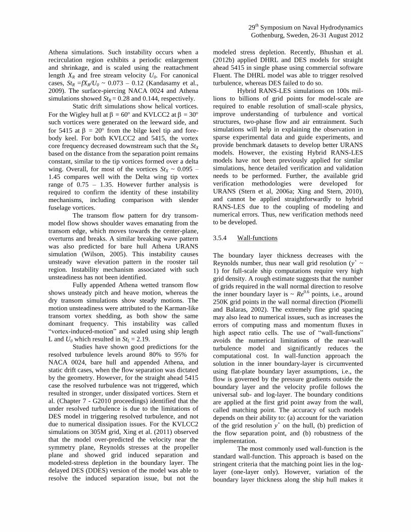
Flapping instability was predicted for the free-
surface separation bubble in surface-piercing NACA
0024 simulations, and transom wake for bare hull
29th
Symposium on Naval Hydrodynamics
Gothenburg, Sweden, 26-31 August 2012
Athena simulations. Such instability occurs when a
recirculation region exhibits a periodic enlargement
and shrinkage, and is scaled using the reattachment
length XR and free stream velocity U0. For canonical
cases, StR =fXR/U0 ~ 0.073 – 0.12 (Kandasamy et al.,
2009). The surface-piercing NACA 0024 and Athena
simulations showed StR = 0.28 and 0.144, respectively.
Static drift simulations show helical vortices.
For the Wigley hull at = 60 and KVLCC2 at = 30
such vortices were generated on the leeward side, and
for 5415 at = 20 from the bilge keel tip and fore-
body keel. For both KVLCC2 and 5415, the vortex
core frequency decreased downstream such that the StX
based on the distance from the separation point remains
constant, similar to the tip vortices formed over a delta
wing. Overall, for most of the vortices StX ~ 0.095 –
1.45 compares well with the Delta wing tip vortex
range of 0.75 – 1.35. However further analysis is
required to confirm the identity of these instability
mechanisms, including comparison with slender
fuselage vortices.
The transom flow pattern for dry transom-
model flow shows shoulder waves emanating from the
transom edge, which moves towards the center-plane,
overturns and breaks. A similar breaking wave pattern
was also predicted for bare hull Athena URANS
simulation (Wilson, 2005). This instability causes
unsteady wave elevation pattern in the rooster tail
region. Instability mechanism associated with such
unsteadiness has not been identified.
Fully appended Athena wetted transom flow
shows unsteady pitch and heave motion, whereas the
dry transom simulations show steady motions. The
motion unsteadiness were attributed to the Karman-like
transom vortex shedding, as both show the same
dominant frequency. This instability was called
“vortex-induced-motion” and scaled using ship length
L and U0 which resulted in StL = 2.19.
Studies have shown good predictions for the
resolved turbulence levels around 80% to 95% for
NACA 0024, bare hull and appended Athena, and
static drift cases, when the flow separation was dictated
by the geometry. However, for the straight ahead 5415
case the resolved turbulence was not triggered, which
resulted in stronger, under dissipated vortices. Stern et
al. (Chapter 7 - G2010 proceedings) identified that the
under resolved turbulence is due to the limitations of
DES model in triggering resolved turbulence, and not
due to numerical dissipation issues. For the KVLCC2
simulations on 305M grid, Xing et al. (2011) observed
that the model over-predicted the velocity near the
symmetry plane, Reynolds stresses at the propeller
plane and showed grid induced separation and
modeled-stress depletion in the boundary layer. The
delayed DES (DDES) version of the model was able to
resolve the induced separation issue, but not the
modeled stress depletion. Recently, Bhushan et al.
(2012b) applied DHRL and DES models for straight
ahead 5415 in single phase using commercial software
Fluent. The DHRL model was able to trigger resolved
turbulence, whereas DES failed to do so.
Hybrid RANS-LES simulations on 100s mil-
lions to billions of grid points for model-scale are
required to enable resolution of small-scale physics,
improve understanding of turbulence and vortical
structures, two-phase flow and air entrainment. Such
simulations will help in explaining the observation in
sparse experimental data and guide experiments, and
provide benchmark datasets to develop better URANS
models. However, the existing Hybrid RANS-LES
models have not been previously applied for similar
simulations, hence detailed verification and validation
needs to be performed. Further, the available grid
verification methodologies were developed for
URANS (Stern et al, 2006a; Xing and Stern, 2010),
and cannot be applied straightforwardly to hybrid
RANS-LES due to the coupling of modeling and
numerical errors. Thus, new verification methods need
to be developed.
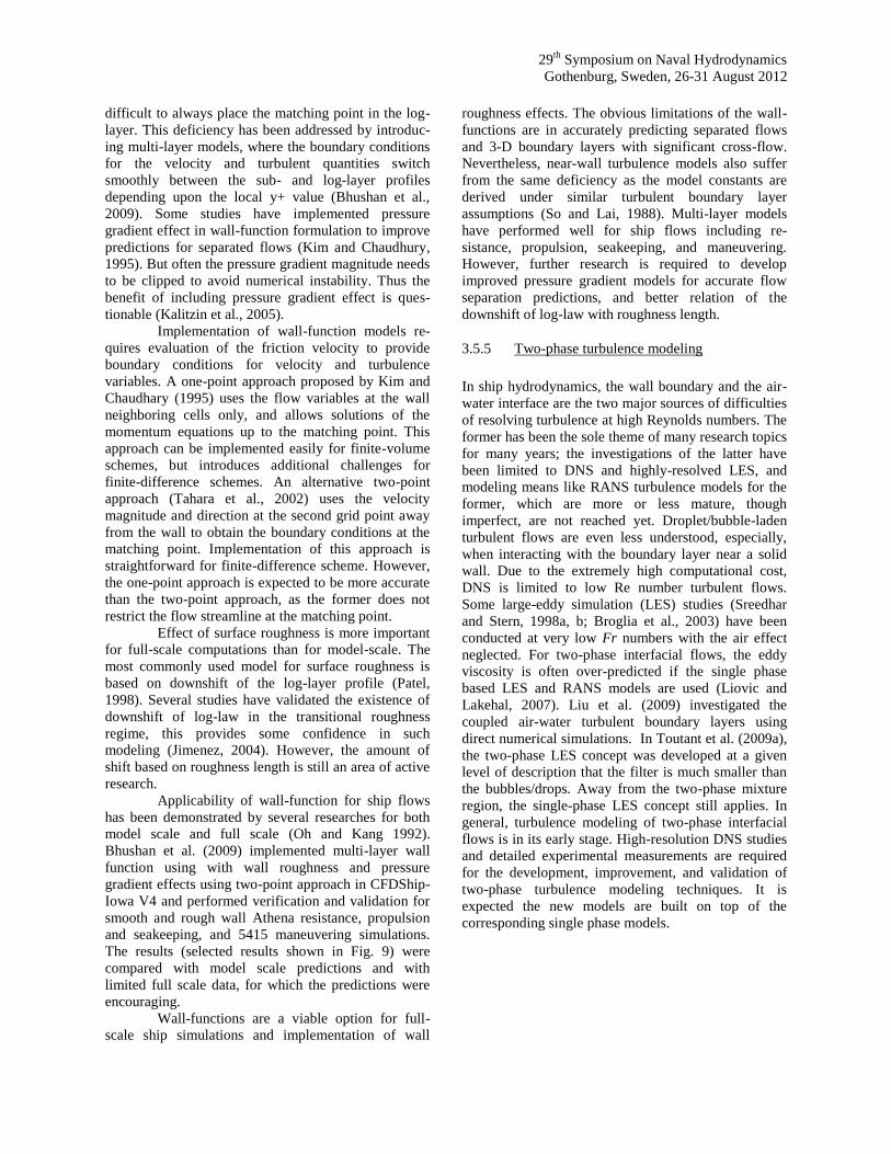
3.5.4 Wall-functions
The boundary layer thickness decreases with the
Reynolds number, thus near wall grid resolution (y+ ~
1) for full-scale ship computations require very high
grid density. A rough estimate suggests that the number
of grids required in the wall normal direction to resolve
the inner boundary layer is ~ Re0.6
points, i.e., around
250K grid points in the wall normal direction (Piomelli
and Balaras, 2002). The extremely fine grid spacing
may also lead to numerical issues, such as increases the
errors of computing mass and momentum fluxes in
high aspect ratio cells. The use of “wall-functions”
avoids the numerical limitations of the near-wall
turbulence model and significantly reduces the
computational cost. In wall-function approach the
solution in the inner boundary-layer is circumvented
using flat-plate boundary layer assumptions, i.e., the
flow is governed by the pressure gradients outside the
boundary layer and the velocity profile follows the
universal sub- and log-layer. The boundary conditions
are applied at the first grid point away from the wall,
called matching point. The accuracy of such models
depends on their ability to: (a) account for the variation
of the grid resolution y+ on the hull, (b) prediction of
the flow separation point, and (b) robustness of the
implementation.
The most commonly used wall-function is the
standard wall-function. This approach is based on the
stringent criteria that the matching point lies in the log-
layer (one-layer only). However, variation of the
boundary layer thickness along the ship hull makes it
29th
Symposium on Naval Hydrodynamics
Gothenburg, Sweden, 26-31 August 2012
difficult to always place the matching point in the log-
layer. This deficiency has been addressed by introduc-
ing multi-layer models, where the boundary conditions
for the velocity and turbulent quantities switch
smoothly between the sub- and log-layer profiles
depending upon the local y+ value (Bhushan et al.,
2009). Some studies have implemented pressure
gradient effect in wall-function formulation to improve
predictions for separated flows (Kim and Chaudhury,
1995). But often the pressure gradient magnitude needs
to be clipped to avoid numerical instability. Thus the
benefit of including pressure gradient effect is ques-
tionable (Kalitzin et al., 2005).
Implementation of wall-function models re-
quires evaluation of the friction velocity to provide
boundary conditions for velocity and turbulence
variables. A one-point approach proposed by Kim and
Chaudhary (1995) uses the flow variables at the wall
neighboring cells only, and allows solutions of the
momentum equations up to the matching point. This
approach can be implemented easily for finite-volume
schemes, but introduces additional challenges for
finite-difference schemes. An alternative two-point
approach (Tahara et al., 2002) uses the velocity
magnitude and direction at the second grid point away
from the wall to obtain the boundary conditions at the
matching point. Implementation of this approach is
straightforward for finite-difference scheme. However,
the one-point approach is expected to be more accurate
than the two-point approach, as the former does not
restrict the flow streamline at the matching point.
Effect of surface roughness is more important
for full-scale computations than for model-scale. The
most commonly used model for surface roughness is
based on downshift of the log-layer profile (Patel,
1998). Several studies have validated the existence of
downshift of log-law in the transitional roughness
regime, this provides some confidence in such
modeling (Jimenez, 2004). However, the amount of
shift based on roughness length is still an area of active
research.
Applicability of wall-function for ship flows
has been demonstrated by several researches for both
model scale and full scale (Oh and Kang 1992).
Bhushan et al. (2009) implemented multi-layer wall
function using with wall roughness and pressure
gradient effects using two-point approach in CFDShip-
Iowa V4 and performed verification and validation for
smooth and rough wall Athena resistance, propulsion
and seakeeping, and 5415 maneuvering simulations.
The results (selected results shown in Fig. 9) were
compared with model scale predictions and with
limited full scale data, for which the predictions were
encouraging.
Wall-functions are a viable option for full-
scale ship simulations and implementation of wall
roughness effects. The obvious limitations of the wall-
functions are in accurately predicting separated flows
and 3-D boundary layers with significant cross-flow.
Nevertheless, near-wall turbulence models also suffer
from the same deficiency as the model constants are
derived under similar turbulent boundary layer
assumptions (So and Lai, 1988). Multi-layer models
have performed well for ship flows including re-
sistance, propulsion, seakeeping, and maneuvering.
However, further research is required to develop
improved pressure gradient models for accurate flow
separation predictions, and better relation of the
downshift of log-law with roughness length.
3.5.5 Two-phase turbulence modeling
In ship hydrodynamics, the wall boundary and the air-
water interface are the two major sources of difficulties
of resolving turbulence at high Reynolds numbers. The
former has been the sole theme of many research topics
for many years; the investigations of the latter have
been limited to DNS and highly-resolved LES, and
modeling means like RANS turbulence models for the
former, which are more or less mature, though
imperfect, are not reached yet. Droplet/bubble-laden
turbulent flows are even less understood, especially,
when interacting with the boundary layer near a solid
wall. Due to the extremely high computational cost,
DNS is limited to low Re number turbulent flows.
Some large-eddy simulation (LES) studies (Sreedhar
and Stern, 1998a, b; Broglia et al., 2003) have been
conducted at very low Fr numbers with the air effect
neglected. For two-phase interfacial flows, the eddy
viscosity is often over-predicted if the single phase
based LES and RANS models are used (Liovic and
Lakehal, 2007). Liu et al. (2009) investigated the
coupled air-water turbulent boundary layers using
direct numerical simulations. In Toutant et al. (2009a),
the two-phase LES concept was developed at a given
level of description that the filter is much smaller than
the bubbles/drops. Away from the two-phase mixture
region, the single-phase LES concept still applies. In
general, turbulence modeling of two-phase interfacial
flows is in its early stage. High-resolution DNS studies
and detailed experimental measurements are required
for the development, improvement, and validation of
two-phase turbulence modeling techniques. It is
expected the new models are built on top of the
corresponding single phase models.
29th
Symposium on Naval Hydrodynamics
Gothenburg, Sweden, 26-31 August 2012
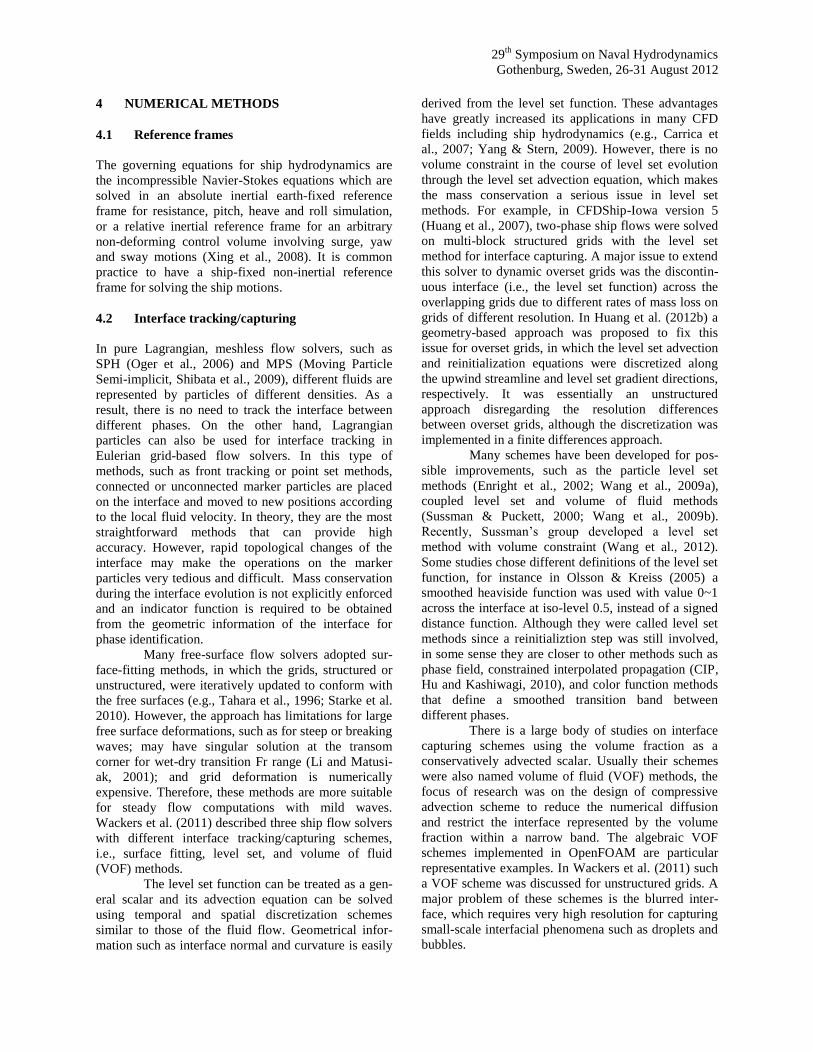
4 NUMERICAL METHODS
4.1 Reference frames
The governing equations for ship hydrodynamics are
the incompressible Navier-Stokes equations which are
solved in an absolute inertial earth-fixed reference
frame for resistance, pitch, heave and roll simulation,
or a relative inertial reference frame for an arbitrary
non-deforming control volume involving surge, yaw
and sway motions (Xing et al., 2008). It is common
practice to have a ship-fixed non-inertial reference
frame for solving the ship motions.
4.2 Interface tracking/capturing
In pure Lagrangian, meshless flow solvers, such as
SPH (Oger et al., 2006) and MPS (Moving Particle
Semi-implicit, Shibata et al., 2009), different fluids are
represented by particles of different densities. As a
result, there is no need to track the interface between
different phases. On the other hand, Lagrangian
particles can also be used for interface tracking in
Eulerian grid-based flow solvers. In this type of
methods, such as front tracking or point set methods,
connected or unconnected marker particles are placed
on the interface and moved to new positions according
to the local fluid velocity. In theory, they are the most
straightforward methods that can provide high
accuracy. However, rapid topological changes of the
interface may make the operations on the marker
particles very tedious and difficult. Mass conservation
during the interface evolution is not explicitly enforced
and an indicator function is required to be obtained
from the geometric information of the interface for
phase identification.
Many free-surface flow solvers adopted sur-
face-fitting methods, in which the grids, structured or
unstructured, were iteratively updated to conform with
the free surfaces (e.g., Tahara et al., 1996; Starke et al.
2010). However, the approach has limitations for large
free surface deformations, such as for steep or breaking
waves; may have singular solution at the transom
corner for wet-dry transition Fr range (Li and Matusi-
ak, 2001); and grid deformation is numerically
expensive. Therefore, these methods are more suitable
for steady flow computations with mild waves.
Wackers et al. (2011) described three ship flow solvers
with different interface tracking/capturing schemes,
i.e., surface fitting, level set, and volume of fluid
(VOF) methods.
The level set function can be treated as a gen-
eral scalar and its advection equation can be solved
using temporal and spatial discretization schemes
similar to those of the fluid flow. Geometrical infor-
mation such as interface normal and curvature is easily
derived from the level set function. These advantages
have greatly increased its applications in many CFD
fields including ship hydrodynamics (e.g., Carrica et
al., 2007; Yang & Stern, 2009). However, there is no
volume constraint in the course of level set evolution
through the level set advection equation, which makes
the mass conservation a serious issue in level set
methods. For example, in CFDShip-Iowa version 5
(Huang et al., 2007), two-phase ship flows were solved
on multi-block structured grids with the level set
method for interface capturing. A major issue to extend
this solver to dynamic overset grids was the discontin-
uous interface (i.e., the level set function) across the
overlapping grids due to different rates of mass loss on
grids of different resolution. In Huang et al. (2012b) a
geometry-based approach was proposed to fix this
issue for overset grids, in which the level set advection
and reinitialization equations were discretized along
the upwind streamline and level set gradient directions,
respectively. It was essentially an unstructured
approach disregarding the resolution differences
between overset grids, although the discretization was
implemented in a finite differences approach.
Many schemes have been developed for pos-
sible improvements, such as the particle level set
methods (Enright et al., 2002; Wang et al., 2009a),
coupled level set and volume of fluid methods
(Sussman & Puckett, 2000; Wang et al., 2009b).
Recently, Sussman’s group developed a level set
method with volume constraint (Wang et al., 2012).
Some studies chose different definitions of the level set
function, for instance in Olsson & Kreiss (2005) a
smoothed heaviside function was used with value 0~1
across the interface at iso-level 0.5, instead of a signed
distance function. Although they were called level set
methods since a reinitializtion step was still involved,
in some sense they are closer to other methods such as
phase field, constrained interpolated propagation (CIP,
Hu and Kashiwagi, 2010), and color function methods
that define a smoothed transition band between
different phases.
There is a large body of studies on interface
capturing schemes using the volume fraction as a
conservatively advected scalar. Usually their schemes
were also named volume of fluid (VOF) methods, the
focus of research was on the design of compressive
advection scheme to reduce the numerical diffusion
and restrict the interface represented by the volume
fraction within a narrow band. The algebraic VOF
schemes implemented in OpenFOAM are particular
representative examples. In Wackers et al. (2011) such
a VOF scheme was discussed for unstructured grids. A
major problem of these schemes is the blurred inter-
face, which requires very high resolution for capturing
small-scale interfacial phenomena such as droplets and
bubbles.
29th
Symposium on Naval Hydrodynamics
Gothenburg, Sweden, 26-31 August 2012
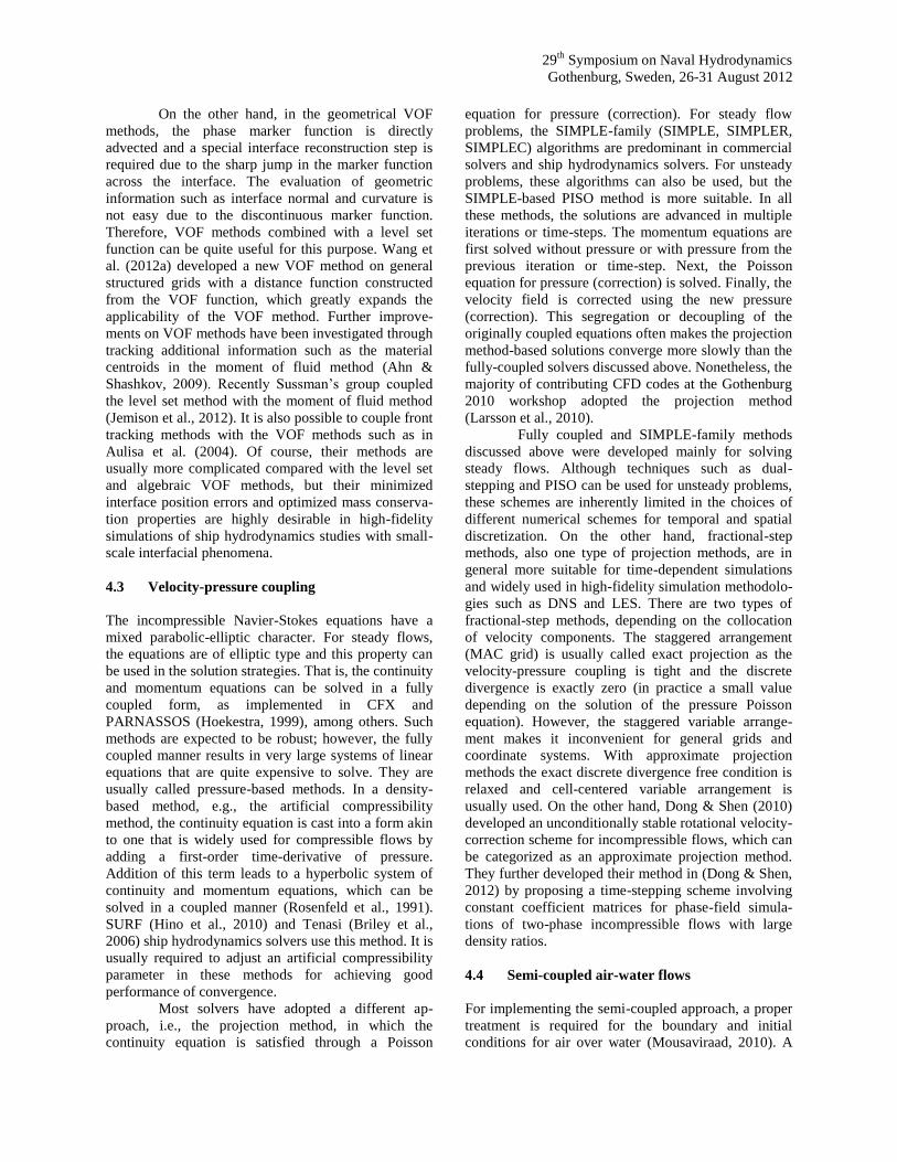
On the other hand, in the geometrical VOF
methods, the phase marker function is directly
advected and a special interface reconstruction step is
required due to the sharp jump in the marker function
across the interface. The evaluation of geometric
information such as interface normal and curvature is
not easy due to the discontinuous marker function.
Therefore, VOF methods combined with a level set
function can be quite useful for this purpose. Wang et
al. (2012a) developed a new VOF method on general
structured grids with a distance function constructed
from the VOF function, which greatly expands the
applicability of the VOF method. Further improve-
ments on VOF methods have been investigated through
tracking additional information such as the material
centroids in the moment of fluid method (Ahn &
Shashkov, 2009). Recently Sussman’s group coupled
the level set method with the moment of fluid method
(Jemison et al., 2012). It is also possible to couple front
tracking methods with the VOF methods such as in
Aulisa et al. (2004). Of course, their methods are
usually more complicated compared with the level set
and algebraic VOF methods, but their minimized
interface position errors and optimized mass conserva-
tion properties are highly desirable in high-fidelity
simulations of ship hydrodynamics studies with small-
scale interfacial phenomena.
4.3 Velocity-pressure coupling
The incompressible Navier-Stokes equations have a
mixed parabolic-elliptic character. For steady flows,
the equations are of elliptic type and this property can
be used in the solution strategies. That is, the continuity
and momentum equations can be solved in a fully
coupled form, as implemented in CFX and
PARNASSOS (Hoekestra, 1999), among others. Such
methods are expected to be robust; however, the fully
coupled manner results in very large systems of linear
equations that are quite expensive to solve. They are
usually called pressure-based methods. In a density-
based method, e.g., the artificial compressibility
method, the continuity equation is cast into a form akin
to one that is widely used for compressible flows by
adding a first-order time-derivative of pressure.
Addition of this term leads to a hyperbolic system of
continuity and momentum equations, which can be
solved in a coupled manner (Rosenfeld et al., 1991).
SURF (Hino et al., 2010) and Tenasi (Briley et al.,
2006) ship hydrodynamics solvers use this method. It is
usually required to adjust an artificial compressibility
parameter in these methods for achieving good
performance of convergence.
Most solvers have adopted a different ap-
proach, i.e., the projection method, in which the
continuity equation is satisfied through a Poisson
equation for pressure (correction). For steady flow
problems, the SIMPLE-family (SIMPLE, SIMPLER,
SIMPLEC) algorithms are predominant in commercial
solvers and ship hydrodynamics solvers. For unsteady
problems, these algorithms can also be used, but the
SIMPLE-based PISO method is more suitable. In all
these methods, the solutions are advanced in multiple
iterations or time-steps. The momentum equations are
first solved without pressure or with pressure from the
previous iteration or time-step. Next, the Poisson
equation for pressure (correction) is solved. Finally, the
velocity field is corrected using the new pressure
(correction). This segregation or decoupling of the
originally coupled equations often makes the projection
method-based solutions converge more slowly than the
fully-coupled solvers discussed above. Nonetheless, the
majority of contributing CFD codes at the Gothenburg
2010 workshop adopted the projection method
(Larsson et al., 2010).
Fully coupled and SIMPLE-family methods
discussed above were developed mainly for solving
steady flows. Although techniques such as dual-
stepping and PISO can be used for unsteady problems,
these schemes are inherently limited in the choices of
different numerical schemes for temporal and spatial
discretization. On the other hand, fractional-step
methods, also one type of projection methods, are in
general more suitable for time-dependent simulations
and widely used in high-fidelity simulation methodolo-
gies such as DNS and LES. There are two types of
fractional-step methods, depending on the collocation
of velocity components. The staggered arrangement
(MAC grid) is usually called exact projection as the
velocity-pressure coupling is tight and the discrete
divergence is exactly zero (in practice a small value
depending on the solution of the pressure Poisson
equation). However, the staggered variable arrange-
ment makes it inconvenient for general grids and
coordinate systems. With approximate projection
methods the exact discrete divergence free condition is
relaxed and cell-centered variable arrangement is
usually used. On the other hand, Dong & Shen (2010)
developed an unconditionally stable rotational velocity-
correction scheme for incompressible flows, which can
be categorized as an approximate projection method.
They further developed their method in (Dong & Shen,
2012) by proposing a time-stepping scheme involving
constant coefficient matrices for phase-field simula-
tions of two-phase incompressible flows with large
density ratios.
4.4 Semi-coupled air-water flows
For implementing the semi-coupled approach, a proper
treatment is required for the boundary and initial
conditions for air over water (Mousaviraad, 2010). A
29th
Symposium on Naval Hydrodynamics
Gothenburg, Sweden, 26-31 August 2012
potential solution is obtained for air over water waves
which have a discontinuity since the tangential velocity
changes sign across the surface. Then a blending
function is introduced to treat the discontinuity in the
potential solution and roughly represent the thin
viscous layer above the water waves. For irregular
waves, the same potential solution and blending
function is used to define each elementary wave
component in the superposition.
The semi-coupled approach in CFDShip-Iowa
V4.5 is used to study the effects of head winds on ship
forces, moments, motions, and airwake flows for calm
water straight ahead, static drift, and dynamic PMM
maneuvers of the ONR tumblehome with validations
against wind towing tank experiments (Mousaviraad et
al., 2012). Figure 10 shows examples of the air flow
field results for static conditions. Computations are
also carried out for pitch and heave in regular head
waves and 6DOF motions in irregular waves simulat-
ing hurricane CAMILLE (Mousaviraad et al., 2008).
Thermal and concentration transport models are
implemented in CFDShip-Iowa version 4.5 (Huang et
al., 2010) to investigate the exhaust plume around ship
superstructures. Figure 11 shows exhaust plume of the
ONR Tumblehome in an extreme motions condition.
Complicated vortical structures are observed in air
including a pair of counter-rotating vortices down-
stream of the stack for cross-flow, and bended bird-
plume shape in the symmetry plane and varying arc-
shape in axial sections both for temperature and NOx
concentration fields.
4.5 Spatial discretization
The discretization of the governing equations are
performed either using finite-volume (FV) or finite-
difference (FD) approach. A survey of the G2010
submissions shows that the FV approach is more
common in ship hydrodynamics community than FD
approached (Larsson et al., 2010). This is because FV
approach can be applied for arbitrary polyhedral grid
volumes which are easier to generate than curvilinear
structured grids required for FD. However, FV
methods are not suited for implementation of higher
order schemes and mostly use second-order schemes.
On the other hand, FD approach allows implementation
of 3rd-order and 5th-order schemes with ease (Yang &
Stern, 2009). The diffusion terms are mostly discre-
tized using central-differencing, whereas upwind-
biased schemes are used for convective terms. Higher-
order schemes provide better accuracy, yet often at the
expense of additional numerical cost and solution
instability. Numerical methods often include flux-
limiter or slope-limiter designed to suppress unphysical
oscillations in solutions (Ismail et al., 2010).
4.6 Temporal discretization
The majority of CFD solvers use implicit time-
marching schemes. Implicit time-marching schemes
allow one to use much larger time-step size than
explicit time-marching schemes, speeding up numeri-
cal solutions for flows with large characteristic time
scales. Implicit time-marching, however, requires
solutions of system of coupled non-linear equations,
which incur computational cost. Explicit time-
marching, which forces much smaller time-step size, is
rarely used for RANS computations. Time step
discretization is achieved by using first-order backward
Euler scheme for steady-state cases, and second-order
schemes such as Crank-Nicolson and three-level
backward schemes for time-accurate solutions (Larsson
et al., 2010). Limited studies have used 4th-order
Runge-Kutta schemes. Studies often use solution
relaxation to improve stability of the solution.
4.7 Semi-Lagrangian advection schemes
In general, high Reynolds number turbulent flows are
advection dominated. Therefore, the advection schemes
used for the momentum equation are critical for the
accuracy of simulations. Higher-order advection
schemes are difficult to be made implicit in time. Thus
treatments like deferred corrections are quite popular in
engineering CFD solvers, because explicit Eulerian
advection schemes are subject to the CFL number for
time step restriction. When the flow velocity is high
and/or the grid spacing is small, the CFL restriction
due to the time step from the explicit advection
schemes can be prohibitive. Semi-Lagrangian advec-
tion schemes have been enjoyed for a long time in the
numerical weather prediction community. With these
unconditionally stable schemes, higher-order spa-
tial/temporal accuracy can be retained and significantly
increased maximum allowable time steps with CFL
numbers up to 4~5 can be safely used. In Xiu &
Karniadakis (2001), a high-order semi-Lagrangian
spectral element method was developed for incom-
pressible flows. Recently, Wang et al. (2012b)
developed a semi-Lagrangian advection scheme for the
VOF method, which are more accurate than the
corresponding Eulerian scheme and much improved
with regard to mass conservation. With the increased
popularity of adaptive mesh refinement techniques,
more and more studies of semi-Lagrangian schemes
have been conducted. Min and Gibou (2006) developed
a second-order projection method using a semi-
Lagrangian advection scheme for incompressible flows
on adaptive Cartesian grids. They also reported a
second-order semi-Lagrangian level set method on
adaptive grids later (Min and Gibou, 2007). Most
recent studies have been focused on conservative semi-
29th
Symposium on Naval Hydrodynamics
Gothenburg, Sweden, 26-31 August 2012
Lagrangian advection schemes, such as Lentine et al.
(2011) and Qiu & Shu (2011).
4.8 Grid generation
Numerical grids are categorized into Cartesian,
structured and unstructured. Most solvers in ship
hydrodynamics community including both research and
application solvers use unstructured grids wherein the
fluid region is sub-divided into tetrahedral cells in the
boundary layer and polyhedral cells elsewhere
(Marcum, 1995). Octree subdivision, Delaunay point
insertion, and advancing front techniques are used to
create the tetrahedral cells near the wall. These grids
are relatively easy to make for complex geometry, but
it is difficult to control the grid quality (Baker et al.,
1989). Structured grids use body fitted hexahedral
cells, and are quite complicated to generate for
complex geometries (Thompson et al., 1985). Elliptical
smoothing algorithms are often used to improve the
quality of the grids. These structured grids are used
along with multi-block overset grid techniques to ease
the grid generation complexity. Multi-block techniques
use topological inter-connections to connect the faces
of the blocks. This can be done using overset or
overlapping techniques, where the interpolation is
applied across local cell volumes and faces. These
interpolation schemes can be applied dynamically to
form transient moving and sliding grids to account for
the relative motions of the ship hull and the rotation of
the propulsion system and appendages (Noack, 2006;
Wang and Parthasarthy, 2000). The Cartesian grid
methods and upcoming technology are discussed
separately.
4.9 Solution adaptation
Solution adaptation in CFD is the process in which the
computational approaches are modified during the
solution process of a given problem, in order to obtain
a more accurate description of the fluid flow or
maintain a similar order of accuracy but with reduced
computational cost. There are four types of solution
adaptation strategies: i) m-adaption, in which different
mathematical models are used within different portions
of the computational domain, for example, the coupling
of a potential solver and a viscous solver for ship
flows, the coupling of an Euler solver and a Navier-
Stokes solver for aerodynamic flows, also, the coupling
of RANS models within the boundary layer and LES in
the bulk flow in a hybrid RANS/LES simulation; ii) p-
adaption, in which discretization schemes of different
orders are used in different portions of the computa-
tional domain, for instance, in finite element methods
the p-adaptive strategy is frequently used with different
shape functions represented by different orders of
polynomials in each element; iii) r-adaption, in which
the grid points are allowed to move, but without
changing the grid connectivity, in the solution process
to give better resolution to an interested area; and iv) h-
adaption, in which grids points are added or deleted by
changing the grid connectivity. The h-adaption is the
most popular approach as there are no coupling issues
between different mathematical models and discretiza-
tion schemes and it is not limited by the initial number
of grid points and the difficulty of grid quality control
as in the r-adaption. Overset grid techniques can be
used to obtain h-adaption, but usually the refinement
regions such as the free surface and wake are deter-
mined beforehand instead of adaptively during the
computations due to the extra computational overhead
of grid oversetting procedure (Carrica et al., 2007). A
directional adaptive mesh refinement method was
developed in Wackers et al. (2012) in ISIS-CFD using
unstructured hexahedral finite volume meshes.
The solution adaptation processes require the
evaluation of adaptation metric to identify the regions
of interest. The choice of adaptation metric depends on
the application. The simplest techniques define the
solution adaptation region based on the experience and
knowledge of the user, for example wake planes or
wave surfaces. Vorticity is often used for improved
vortex-core resolution. Other methods include feature-
detection where the feature of interest is associated
with a flow regime or specific characteristic or
property. For example, in turbulent flows the following
metrics have been used: Q-criterion, λ2, λci, and λ+
(Hunt et al., 1988; Jeong and Hussain, 1995; Horiuti,
2003). The Q-criterion uses the rotation rate tensor to
refine the mesh around areas of high rotation. The λ2
metric seeks to capture pressure minima. λci metric
refines the mesh based on the velocity gradient tensor.
Finally, the λ+ metric works by calculating the
strainrate-vorticity correlation. Both h- and r-adaption
methods as well as hybrid approaches have been used
successfully for improved flow feature detection, local
reduction in discretization error, and convergence to an
optimal grid.
4.10 Cartesian grid methods
Several Cartesian grid methods were presented for ship
wave problems in the literature. Miyata et al. (1985b)
developed a modified Marker and Cell method
(TUMMAC) for the finite difference solution of non-
linear wave generation in the near field of ships. A
Cartesian grid approach was presented in (Sussman and
Dommermuth, 2000) with a coupled level-set/volume-
of-fluid method for interface capturing and an embed-
ded boundary method for the immersed geometry.
They also reported another approach using immersed-
body and volume-of-fluid methods and its recent
29th
Symposium on Naval Hydrodynamics
Gothenburg, Sweden, 26-31 August 2012
development was given in Dommermuth et al. (2007)
for ship wave simulations. Hu et al. (2010) developed a
CIP based Cartesian grid method for numerical
simulation of strongly nonlinear wave-ship interaction.
Yang & Stern (2009) developed a coupled immersed-
boundary/level-set method for wave-body interactions.
A second-order sharp interface immersed boundary
method was used for two-phase flows with multiple
moving bodies on fixed Cartesian grids. A ghost-fluid
method is used without smearing the density across the
fluid-fluid interface. This method was applied in the
study of ship model DTMB 5512 at Fr=0.41 in Yang et
al. (2008b). The instantaneous air-water interface
colored by the elevation is shown in Fig. 12. The
breaking bow waves and scars induced by them are
evident. Figure 13 shows the instantaneous vortical
structures colored by streamwise vorticity in the air
flow. There are many Cartesian grid methods for other
areas of applications, the reader is referred to Yang &
Stern (2009) for related discussions and references
therein.
On the other hand, the application of Cartesian
grid methods can become practically prohibitive for
high Reynolds number flows due to the demanding
resolution requirement near the wall boundary, since
most of Cartesian grid methods approximate the
velocity field near the wall boundary by a linear
distribution, which is only correct in the viscous
sublayer. For example, in order to resolve the viscous
sublayer for a turbulent flow case at Re = 106, the near-
wall grid spacing has to be in the range of 10-5
L (L is
the reference length), and the total number of grid
points will be more than a few billions. Therefore,
some forms of wall-layer models have to be included
such that the effects of boundary layer can be taken
into account properly.
4.11 High-fidelity curvilinear grid solvers
Cartesian grids have some desirable properties not
available in other types of grids, especially, triangles
(2D) and tetrahedra (3D). For example, the errors
introduced in the discretization of diffusion terms can
be cancelled out completely at two opposite cell faces;
higher order schemes can be implemented much easier;
also, automatic generation of Cartesian grids with local
refinement is much simpler than that of triangles or
tetrahedral. Therefore, it is preferred to use Cartesian
grids wherever possible and use other types of grids
elsewhere. For instance, Karman & Wilson (2008)
developed an automatic grid generation algorithm
based on octree refinement Cartesian grid with general
cutting allowing viscous boundary layer grid genera-
tion. Their development was implemented in Tenasi, a
general purpose unstructured grid solver for a wide
range of applications.
On the other hand, usually it is not necessary
to pursue such level of universality, e.g., using
unstructured grids with all types of grid elements, for
ship hydrodynamics applications, since the geometries
are more or less confined to hull forms, appendages,
and propellers of a limited range of variations. Once
the surface topology of a geometrical object is
determined, a nearly-optimized surface decomposition
can be obtained and the corresponding surface
quadrilateral grid can be generated with usually good
orthogonality, not to mention that most shapes have
been given as parameterized solid modeling surfaces
which are readily dividable in u - v coordinates during
the design process. This also explains why structured
grids are still predominately used in computational ship
hydrodynamics.
In addition, high-order schemes can be easily
implemented in structured grids. For example, in Suh
et al. (2011) and Wang et al. (2012c), the Cartesian
grid solver CFDShip-Iowa V6.1 was extended into an
orthogonal curvilinear solver (V6.2) with similar
accuracy and efficiency, where turbulent boundary
layers and small droplets/bubbles are resolved at once.
Numerical methods and HPC components in V6.2 are
about the same as in V6.1. It uses a recently developed
novel volume-of-fluid method for general structured
grids with a constructed level set function (Wang et al.,
2012a), thus it can be used for detailed simulations of
interfacial phenomena such as wave breaking and
wave-body interactions with simple geometries like
cylinder, sphere, wedge, foil, etc. The orthogonal
curvilinear grid solver has been used for studying the
high Reynolds number, high Froude number turbulent
flow past an interface-piercing circular cylinder and a
wedge-shaped bow. In addition, an overset grid solver,
CFDShip-Iowa V6.2.5, was presented in Bhushan et al.
(2011b), which couples the Cartesain grid solver and
the orthogonal curvilinear grid solver via overset grid
package SUGGAR (Noack, 2006). Based on the
Cartesian grid solver and the orthogonal curvilinear
grid solver, a general multi-block structured grid solver
(V6.3) is currently being developed (Yang et al., 2012).
It maintains and extends the higher-order advection and
volume conservative interface tracking schemes, and
enhanced capabilities of handling complex geometries
in ship hydrodynamics. One additional complication besides the air-
water interface and high-Re boundary layer that has to
be considered is the motions of a ship and its control
surfaces and propellers (when discretized propellers
instead of models are used). Multi-blocked structured
grids, even with moving grid and/or sliding interface
capabilities, are usually considered to be too restricted
for large displacement/angle motions, especially, when
ship-ship interactions are to be addressed. Theoretical-
ly, unstructured grids with grid deformation and
29th
Symposium on Naval Hydrodynamics
Gothenburg, Sweden, 26-31 August 2012
regeneration capabilities can be applicable, but the
computational cost of grid operation could be high,
especially, for running on tens/hundreds or thousands
processes, and the grid quality and algorithm robust-
ness are concerns too. The overset grid techniques have
been very successful in ship flow computations (e.g.,
Carrica et al., 2007); it is expected to continue playing
an important role in future high fidelity ship hydrody-
namics solvers due to its capability and flexibility. Therefore, it is envisioned that the next-
generation, high-fidelity ship hydrodynamics solvers
will be based on Cartesian grids with local/adaptive
refinement capabilities for the bulk flow and immersed
boundary wall modeling techniques or body-fitted
multi-block structured grids for the high-Re boundary
layers. For the latter, overset grid techniques with
improved conservation properties will facilitate grid
connection and movement.
5 HIGH-PERFORMANCE COMPUTING
5.1 HPC advances
Advances in HPC capability, i.e., as the computational
capability doubles every two years as per Moore’s law,
are enabling the use of larger grids and more proces-
sors. However, as the grid size and number of proces-
sors increase, so does the communication time. Further,
HPC hardware architecture is undergoing fundamental
changes. Today’s systems are hybrid clusters of
multicore processors that have shared and distributed
memory inside and across the nodes, respectively. Thus
a parallel algorithm should effectively utilize the
memory of such systems to achieve better performance
(Shalf, 2009). Most ship codes use message passing
interface (MPI) parallelization, which has limitations
on the hybrid networks as the processes running on
different nodes dictate the communication time
(Rabenseifner and Wellein, 2003). Hybrid paralleliza-
tion is well suited for hybrid networks, such as the MPI
for the internode parallelization and open multi-
processing (OpenMP) for the intranode parallellization.
However, the OpenMP implementation overhead often
outweighs the reduction of communication time, but
may be beneficial for codes with substantial collective
communication on high-latency inter-node connection
(Kaushik et al., 2009). Upcoming graphics processing
units (GPUs) can achieve up to 10 times better
performance than the central processing units (CPUs)
and are being applied for CFD (Cohen and Molemaker,
2009). However, they are not yet ready for production
level applications, as multi-GPU and double precision
calculations are still in the developmental stage.
5.2 HPC in computational ship hydrodynamics
Ship hydrodynamics community mostly uses MPI
based domain decomposition, and the HPC efforts are
geared to either run production jobs faster (strong
scalability) or to improve the capability of running
larger jobs that can resolve more physics with less
reliance on modeling (weak scalability). Scalability
studies of free surface CFD codes are scarce and are
dependent on hardware, thus conclusions are difficult
to reach. Overall, incompressible flow codes show
limited strong scalability, i.e., speed up is typically 60
to 80% of the ideal scalability for 1000 processors
(Kremenetsky 2008, Bhushan et al. 2011a). On the
other hand, compressible solvers show linear scalabil-
ity for up to 10’s thousands of processors (Gicquel et
al. 2008). The poor scalability of the incompressible
solvers is due to the solution of pressure Poisson
equation. Weak scalability is usually more easily
achieved and has been the focus of most recent
developments in ship hydrodynamics community.
Static ship computations of hundreds of mil-
lions of grid points have been reported for curvilinear
and Cartesian grid solvers (Bhushan et al. 2011a),
while dynamic moving computations up to 70 million
grid points were performed (Carrica et al. 2010). These
computations enable a degree of detail in the flow
physics that cannot be achieved with coarser grids,
allowing the use of more accurate turbulence models
like hybrid RANS-LES and LES. Computations
including ship motions are harder and limited by the
need of re-gridding or computation of overset connec-
tivity. Computations with motions are routine for grids
ranging between 5 and 25 million grid points. New
promising numerical techniques and hardware
technologies are rapidly changing the landscape of
high-performance computing. Super-scalable Cartesian
grid solvers are breaking the 1 billion grid point limit
with distributed memory platforms (Wang et al.
2012d), and soon 10 and 100 billion grid points will be
possible. The HPC challenges of such solvers are
discussed below.
5.3 HPC challenges
In general, system memory, interconnection, and I/O
are the major bottlenecks in high-fidelity flow simula-
tions. The current norm for system memory is about
2GB/core with around 10% reserved for system usage.
This imposes a hard limit with regard to the degrees of
freedom one core can effectively handle and thus the
minimum number of cores required for a problem of a
given size. In many solvers, some data proportional to
the global size of the problem are used in some stages
of the solution procedure, which further exacerbates
the limit. For instance, many solvers use the root
29th
Symposium on Naval Hydrodynamics
Gothenburg, Sweden, 26-31 August 2012
process to read some initial data such as input infor-
mation and grid data, and then distribute them to other
processes. These data may be of large size and not
containable within the memory capacity of one
computer node. Current computer nodes are usually
equipped with tens of processor cores, ranging from 8
to 64. It is expected that a transition from multi-core to
many-core will be seen in more and more HPC
platforms. The oncoming exascale systems may be
equipped with nodes containing hundreds or even
thousands of cores. It is unlikely the system memory
available to each core will be increased in a scalable
way, and actually the decrease of memory size per core
is more likely to happen due to cost consideration.
Therefore, it is critical to minimize memory usage in
high-fidelity solvers for being able to run them on
tomorrow’s HPC platforms. For this point of view,
Cartesian grid solvers have some particular advantages.
In contrast to curvilinear structured grids or unstruc-
tured grids, only one-dimensional arrays are required
for grid coordinates and Jacobian matrix information.
Also, discretization stencils are far smaller if the same
order-of-accuracy is sought. For example, second-order
finite difference discretization of the Lapacian
operation gives a seven-point stencil on Cartesian
grids, but nineteen-point stencil on general curvilinear
grids. On the other hand, pre-processing steps such as
grid generation could become a major constraint to
solvers for solving billions of degrees of freedom using
curvilinear grids or unstructured grids. With the current
mainstream grid generation techniques, usually done
on a workstation with interactive human input, it is
very difficult to produce billion-point grids. Recently
Wang et al. (2012d) performed high-fidelity simula-
tions of plunging breaking waves behind a bump using
2.2 billion grid points. It was possible to generate a 2D
grid using a commercial grid generator and the 3D grid
was obtained through translational extrusion, thanks to
the simple geometry.
Interconnection performance between com-
puter nodes is constrained by network bandwidth and
communication latency. Because high-fidelity simula-
tions may involve millions of parallel tasks, collective
and synchronization operations, which are usually
unavoidable in many solvers, can become the deter-
mining factor for the overall algorithm scalability. It is
necessary to develop algorithms that can greatly reduce
communication. Currently, there is a clear trend to
change from pure MPI programming mode to hybrid
MPI/OpenMP programming due to the transition of
multi-core CPU toward many-core CPU. Within one
node, the OpenMP mode can avoid MPI communica-
tion latency, reduce request of network bandwidth, and
reduce system memory usage involved in storing
additional ghost cells in pure MPI mode. On the other
hand, implicit schemes usually require many synchro-
nization operations. Semi-Lagrangian advection
schemes could be much advantageous in this regard
because they usually only involve localized operations.
Parallel I/O is another major bottleneck of
high-fidelity simulations. For simulations with billions
of degrees of freedom, it is impossible to use old-
fashioned modes that one or a few nodes read/write all
the files. Similarly, with thousands of nodes, or
millions of cores, the approach in which each
node/core reads/writes its own data files is not
manageable. Even the current MPI I/O is severely
limited in many systems, a major I/O operation such as
writing solution and restart data files using hun-
dreds/thousands of cores may cost the amount of CPU
time for running tens or even hundreds of time steps.
For high-fidelity simulations requiring frequent data
output this could be a major scalability problem, which
could be worse on larger systems as the network and
I/O bandwidths become more congested. Related data
post-processing for high-fidelity simulations also poses
major difficulties. Data visualization and analysis has
to be done on-site or on-the-fly. Data analysis and
reduction within the solvers will become essential
components for mitigating network and I/O bandwidth
requirement of the solvers. Again, compared with
solvers mainly using curvilinear and unstructured grids,
Cartesian grid methods or solvers using mostly
Cartesian grids have some advantages in terms of I/O
when there are changes in grids such as movement,
deformation, and adaption.
6 V&V PROCEDURES
6.1 Background
In spite of the ever-increasing need and importance for
standards for CFD uncertainty analysis/accuracy
estimation and code certification for industrial
applications, there are currently many viewpoints
covering all aspects from basic concepts and defini-
tions to detailed methodology and procedures.
Verification and validation are processes to estimate
the numerical and modeling errors, respectively.
Although the definition of validation is fairly widely
accepted (ASME Performance Test Codes Committee
PTC 61, 2009), many opinions on verification are
controversial. Herein, we focus on quantitative
verification and validation (V&V) methodology and
procedures (Stern et al., 2006a), which are essential
ingredients for the successful implementation of SBD.
Different verification methodologies will be reviewed
and their shortcomings and criticisms will be dis-
cussed.
29th
Symposium on Naval Hydrodynamics
Gothenburg, Sweden, 26-31 August 2012
6.2 Overview of V&V
The approximation used in numerical simulations will
result in error S , which is the difference between a
simulation value S and the truth T . However, the true
values of simulation quantities are rarely known. Thus,
errors must be estimated. An uncertainty U is an
estimate of an error such that the interval U contains
the true value of S 95 times out of 100, i.e., at the
95% confidence level. An uncertainty interval thus
indicates the range of likely magnitudes of S but no
information about its sign.
Sources of errors and uncertainties in
simulation results can be divided into two distinct
sources: modeling and numerical. Modeling errors and
uncertainties are due to assumptions and approxima-
tions in the mathematical representation of the physical
problem (such as geometry, mathematical equation,
coordinate transformation, boundary conditions, air-
water interface, and turbulence models) and incorpora-
tion of previous data (such as fluid properties) into the
model. Numerical errors and uncertainties are due to
numerical solution of the mathematical equations (such
as discretization, artificial dissipation, incomplete
iterative and grid convergence, lack of conservation of
mass, momentum, and energy, internal and external
boundary non-continuity, and computer round-off). In
considering the development and execution of a CFD
code, it is assumed that S is composed of additive
modeling and numerical errors.
S SM SNS T (4)
The simulation uncertainty equation follows directly by
considering equation (4) as a data reduction equation,
as per EFD uncertainty analysis
2 2 2
S SM SNU U U (5)
where SU is the uncertainty in the simulation and SMU
and SNU are the simulation modeling and numerical
uncertainties. It should be noted that correlations
between modeling and numerical errors are also
possible and should be considered in the future.
There are two types of verification. Code veri-
fication is a procedure to find coding mistakes that
affect the numerical discretization using, for example,
the method of manufactured solutions (MMS) (Roache,
2002; Knupp and Salari, 2003). Solution verification is
a process for assessing simulation numerical uncertain-
ties SNU and, when conditions permit, estimating the
sign and magnitude SN of the simulation numerical
error itself and the uncertainties in that error estimate
SNU . The most important numerical errors and
uncertainties are due to use of iterative solution
methods and specification of various input parameters
such as spatial and time-step sizes and other parameters
(e.g., artificial dissipation). The errors and uncertainties
are highly dependent on the specific application
(geometry and conditions). The errors due to specifica-
tion of input parameters are decomposed into error
contributions from iteration number I , grid size
G ,
time step T , and other parameters
P , which gives
the following expressions for the simulation numerical
error and uncertainty.
1
J
SN I G T P j
j
(6)
2 2 2 2 2 2 2
1
J
SN I G T P I j
j
U U U U U U U
(7)
Validation is a process for assessing simulation
modeling uncertainty SMU
by using benchmark
experimental data D and, when conditions permit,
estimating the sign and magnitude of the modeling
error SM itself.
( )D SM SNE D S (8)
2 2 2
V D SNU U U (9)
where E is the comparison error, D D T is the
difference between an experimental data and the truth
and VU is the validation uncertainty. When
| | VE U (10)
the combination of all the errors in D and S is smaller
than VU and validation is achieved at the VU interval.
If VU E , the sign and magnitude of SME can
be used to make modeling improvements..
6.3 Factor of safety method for solution verifica-
tion
Xing and Stern (2010) proposed four steps for solution
verification: (a) convergence studies with four
possibilities: monotonic convergence, oscillatory
convergence; monotonic divergence, and oscillatory
divergence; (b) error estimate SN with magnitude and
sign; (c) uncertainty estimate U that indicates the
range of likely magnitudes of SN , but no information
about its sign; and (d) statistical analysis to establish
that the interval of U at a 95% confidence level
bounds the comparison error E .
29th
Symposium on Naval Hydrodynamics
Gothenburg, Sweden, 26-31 August 2012
Most solution verification methods are de-
rived for monotonic convergence when the general
Richardson extrapolation (RE) method can be used to
estimate the observed order of accuracy REp , error RE ,
and the numerical benchmark CS using three systemat-
ically refined grids. The uncertainty U is defined as an
estimate of an error such that the interval of U , U ,
bounds the true value of SN at a specified level of
confidence, which is usually 95% for experimental
fluid dynamics and CFD. Uncertainty estimates can be
written in the general form of
21
1S p
U Fr
(11)
Various solution verification methods differ in the
choice of factor of safety SF and p. The GCI derived
by Roache (1998) is currently used and recommended
by ASME (Celik, 2008) and AIAA (Cosner et al.,
2006). However, as discussed by Xing and Stern
(2010; 2011), there are different variants of the GCI
method such as the original GCI, GCI1, GCI2, GCI3,
and GCIOR, etc. Thus the choice of SF and p in the
GCI method requires user judgment calls, for which no
single guideline is currently available. The uncertainty
estimate for the original GCI is
21 1.25 | |1RE
GCI S REpU F
r
(12)
The correction factor method (Stern et al.,
2001; Wilson et al., 2004) uses a variable factor of
safety and was validated for correction factor less than
one using a few analytical benchmarks. The factor of
safety for correction factor larger than one is obtained
by assuming that the factor of safety is symmetric with
respect to the asymptotic range where the observed
order of accuracy REp is equal to the theoretical order
of accuracy of the numerical scheme thp ,
1RE thP p p . The uncertainty for the correction
factor method is estimated by the sum of the absolute
value of the improved error estimate | |RECF and the
absolute value of the amount of the correction.
2
9.6 1 1.1 0.875 1.125
2 1 1 0 0.875 1.125
RE
CF
RE
CF CFU
CF CF or CF
(13)
The GCI and CF methods have two deficien-
cies. The first is that the uncertainty estimates for
RE thp p are unreasonably small in comparison to
those with the same distance to the asymptotic range
for RE thp p . This is due to the fact that the error
estimate RE for the former is much smaller than that
of the latter. The second is that there is no statistical
evidence for what confidence level the GCI and CF
methods can actually achieve.
Two other recent studies (Eça and Hoekstra,
2006; Rumsey and Thomas, 2008) considered the use
of different uncertainty estimates for different ranges of
REp for solutions that show monotonic convergence.
These two verification methods were demonstrated for
a manufactured solution (Eça and Hoekstra, 2006) and
the flow over a backward facing step (Eça and
Hoekstra, 2006; Rumsey and Thomas, 2008) without
detailed derivation and validation. Statistical samples
or analyses were not reported in either of these studies.
Recently, Xing and Stern developed the factor
of safety method (Xing and Stern, 2010). It removes
the two deficiencies previously discussed for the GCI
and CF methods. The best error estimate is used to
construct the uncertainty, which is
1 0
1 2
1 0 1
1 1
RE
FS
RE
FS P FS P PU
FS P FS P P
(14)
0 2.45FS , 1 1.6FS , and 2 14.8FS are recom-
mended based on statistical analysis.
6.4 Discussion of the factor of safety method
The factor of safety method is the only solution
verification method that was validated using statistical
analysis, which consists of 25 samples with different
sizes based on 17 studies covering fluids, thermal, and
structure disciplines. Only the factor of safety method,
compared with the GCI and correction factor methods,
provides a reliability larger than 95% and a lower
confidence limit greater than or equal to 1.2 at the 95%
confidence level for the true mean of the parent
population of the actual factor of safety. This conclu-
sion is true for different studies, variables, ranges of P
values, and single P values where multiple actual
factors of safety are available. The number of samples
is large and the range of P values is wide such that the
factor of safety method is also valid for other applica-
tions including results not in the asymptotic range,
which is typical in industrial and fluid engineering
applications. The factor of safety method has been used
to estimate CFD uncertainties in ship hydrodynamics
such as the recent CFD Workshop Gothenburg 2010
(Larsson et al., 2010).
Roache presented ten items of discussion of
the factor of safety method (Roache, 2011), which
29th
Symposium on Naval Hydrodynamics
Gothenburg, Sweden, 26-31 August 2012
were responded item-by-item by Xing and Stern
(2011). Additionally, Xing and Stern (2011) evaluated
two new variants of the GCI method including GCIOR
(Oberkampf and Roy, 2010) and GCI3 methods and
one new variant of the factor of safety method (FS1
method). Except the original GCI method, all variants
of the GCI method have jumps of SF versus P, which
cannot be justified. The FS1 method is the same as the
FS method for 1P but uses thp instead of REp in
the error estimate for 1P . The FS1 method may have
an advantage for uncertainty estimates when 2P
where the FS and other verification methods likely
predict unreasonably small uncertainties due to small
error estimates. However, since the current dataset is
restricted to 2P , the pros/cons of using the FS or
FS1 method cannot be validated. Thus, until additional
data is available for 2P , all verification methods
should be used with caution for such conditions and, if
possible, additional grid-triplet studies conducted to
obtain 2P .
7 V&V FOR CAPTIVE SIMULATIONS
Captive testing in the towing tank is the standard
approach in ship design. The CFD ship hydrodynamic
efforts started with and mostly focused on captive
simulations both to replace the towing tank model
testing and to carry out validations against EFD data.
The CFD community has developed new procedures
for single run captive computations for resistance and
for seakeeping in head waves. The resistance procedure
is not possible or highly difficult using a physical
towing tank suggesting a potential of using CFD to aid
the design process (Xing et al., 2008). The single run
seakeeping procedure is also applicable for experi-
ments or potential flow and can significantly reduce the
costs in all methods (Mousaviraad et al., 2010a). Full-
scale computations are carried out with CFD which are
rarely done in experiments. Appendages are easily
added/removed in CFD simulations and can be used to
study the interactive effects between different append-
ages and the hull. CFD simulations are carried out for
unconventional ships and high speed crafts including
real waterjet flow computations.
This section focuses on CFD captive V&V ef-
forts including resistance, sinkage and trim in calm
water, seakeeping in regular head waves, captive
maneuvering including static and dynamic simulations,
and stability studies.
7.1 Resistance and propulsion
Prediction of resistance is the oldest application of
CFD in ship hydrodynamics and its accuracy has been
significantly improved over the last 20 years. In the
latest workshop on ship hydrodynamics, Gothenburg
2010, a total of 89 submissions of resistance prediction
are documented, which is the largest number in the
workshop series and the analysis of the results shows
that the statistical variance of all the predictions are
substantially smaller than the previous workshops in
2000 and 2005 (2.1% in 2010 compared to 4.7% in
2005) (Larsson & Zou, 2010). An overview of the
computational methods including modeling, numerical
methods, and HPC, and the applications studied are
provided herein, followed by a detailed analysis of
V&V efforts.
The dominate modeling approaches for re-
sistance simulations are RANS for turbulence, while
some simulations are based on LES or DES, surface
capturing methods such as VOF and level-set for free
surface, and unstructured or structured multi-block or
overset grids (Resistance Committee, ITTC 2011;
Larsson & Zou, 2010). Two equation based, isotropic
eddy viscosity turbulence models are most popular,
especially the family of k-ω models. Wall functions for
turbulence modeling are used in some studies, while
many simulations resolve the near wall region includ-
ing the viscous sublayer. The majority of the numerical
methods are based on second order schemes, while
higher order discretization schemes are seldom used.
Gridding techniques include adaptive mesh refinement
and overset grids for moving-body and multi-body
applications as well as local refinement by embedding
blocks of finer grids. The HPC methods have been
vastly used in most recent simulations enabling parallel
computing for increased grid size of a few to tens of
million points to improve the spatial resolution of
turbulent boundary layer and wake.
The resistance prediction simulations are car-
ried out for a wide range of applications and condi-
tions. Other than drag, sinkage and trim, local flow
fields such as boundary layer and wake, and wave
patterns are also predicted by many simulations.
Different geometries including tankers, container ships,
surface combatants, and small vessels are studied at a
range of very small to large Froude numbers. Uncon-
ventional ships such as multi hulls, planing hulls, and
new concept hulls are included, e.g. Bhushan et al.
(2012b) simulations for a SES/ACV ship in deep and
shallow water (Fig. 14). Fully appended ships with
rudders, bilge keels, shafts, struts, and propellers are
also included in the literature. Full-scale resistance
predictions including the effects of surface roughness
have become of interest in the recent years (e.g.
Bhushan et al., 2012c). Mousaviraad et al. (2012)
included the effects of hurricane strength head winds in
their CFD simulations.
Innovative methods are introduced in CFD
studies including a procedure to obtain resistance and
propulsion curves for a wide range of velocities in a
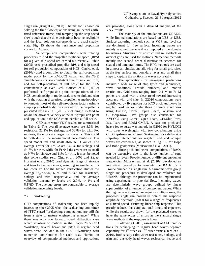
29th
Symposium on Naval Hydrodynamics
Gothenburg, Sweden, 26-31 August 2012
single run (Xing et al., 2008). The method is based on
solving the fluid flow equations using an inertial earth-
fixed reference frame, and ramping up the ship speed
slowly such that the time derivatives become negligible
and the local solution corresponds to a quasi steady-
state. Fig. 15 shows the resistance and propulsion
curves for Athena.
Self-propulsion computations with rotating
propellers to find the propeller rotational speed (RPS)
for a given ship speed are carried out recently. Lubke
(2005) used prescribed propeller RPS and ship speed
for self-propulsion computations of KCS. Carrica et al.
(2010a) used a controller to obtain the self-propulsion
model point for the KVLCC1 tanker and the ONR
Tumblehome surface combatant free to sink and trim,
and for self-propulsion at full scale for the KCS
containership at even keel. Carrica et al. (2010c)
performed self-propulsion point computations of the
KCS containership in model scale free to sink and trim
with the rotating discretized propeller. A methodology
to compute most of the self-propulsion factors using a
simple prescribed body force model for the propeller is
presented by Fu et al. (2010), including a method to
obtain the advance velocity at the self-propulsion point
and application to the KCS containership at full-scale.
CFD calm water V&V results are summarized
in Table 2. The overall average errors are 3.3% for
resistance, 22.2% for sinkage, and 32.8% for trim. For
motions, the errors are larger for lower Fr. This could
be both due to the measurement uncertainties at low
speed model test and small absolute D values. The
average errors for Fr<0.2 are 34.7% for sinkage and
54.7% for trim, while for Fr≥0.2 the errors are as small
as 9.7% for sinkage and 11% for trim. It must be noted
that some studies (e.g. Xing et al., 2008 and Sadat-
Hosseini et al., 2010) used dynamic range of sinkage
and trim to evaluate errors, resulting in smaller errors
for lower Fr. For the limited verification studies the
average USN=2.5%, 6.9% and 6.7%S for resistance,
sinkage and trim, respectively, and the average
validation uncertainty levels are 2.9%, 14.1% and
8.1%D. The average errors are comparable to average
validation uncertainty levels.
7.2 Seakeeping
CFD computations of seakeeping has been rapidly
increasing since 2005 when the seakeeping committee
of ITTC stated “seakeeping computations are still far
from a state of mature engineering science.” While
there was only one forward speed diffraction case
which involves no motions in the Tokyo 2005 CFD
Workshop, several heave and pitch in regular head
waves were included in the G2010 Workshop with
numerous contributions for each case. Herein, an
overview of computational methods and applications
are provided, along with a detailed analysis of the
V&V results.
The majority of the simulations are URANS,
while limited simulations are based on LES or DES.
Surface capturing methods such as VOF and level-set
are dominant for free surface. Incoming waves are
mainly assumed linear and are imposed at the domain
boundaries. Structured or unstructured multi-block or
overset grids are used for motions. Numerical methods
mainly use second order discretization schemes for
spatial and temporal terms. The HPC methods are used
in almost all simulations allowing for small grid sizes
at the free surface and boundary layer and small time
steps to capture the motions in waves accurately.
The applications for seakeeping predictions
include a wide range of ship types and geometries,
wave conditions, Froude numbers, and motion
restrictions. Grid sizes ranging from 0.4 M to 71 M
points are used with a clear trend toward increasing
accuracy with grid size. In G2010 computations were
contributed by five groups for KCS pitch and heave in
regular head waves under three different conditions
using FreSCo, Comet, Open Foam, Wisdam and
CFDShip-Iowa. Five groups also contributed for
KVLCC2 using Comet, Open Foam, CFDShip-Iowa,
Isis, Icare and RIAM-CMEN. A case for pitch and
heave fee to surge was include in G2010 for KVLCC2
with three wavelengths with two contributions using
CFDShip-Iowa and Comet. Seakeeping for side by side
ship-ship interactions for regular head and oblique
waves are carried out, as shown in Fig. 16, for Hope
and Bobo geometries (Mousaviraad et al., 2011).
Since pitch and heave computations of RAOs
can be expensive due to the large number of runs
needed for every Froude number at different encounter
frequencies, Mousaviraad et al. (2010a) developed an
innovative procedure to compute the RAOs for a
Froude number in a single run. A harmonic wave group
single run procedure is developed and validated for
URANS, although the procedure can be implemented
using experiments or potential flow. Incoming waves
are deterministic wave groups defined by linear
superposition of a number of component waves. While
the regular wave procedure requires multiple runs, the
proposed single run procedure obtains the response
amplitude operators (RAO) for a range of frequencies
at a fixed speed, assuming linear ship response. This
greatly reduces the computational time and expenses,
while the results are shown for the presented cases to
have the same order of errors as the standard single
wave methods if the response is linear.
Following G2010, assessment of CFD predic-
tions for seakeeping in regular head waves separate
capability for 1st order vs. 2
nd order terms (Stern et al.,
2010). Both steady calm water resistance, sinkage, and
trim and unsteady head waves resistance, heave and
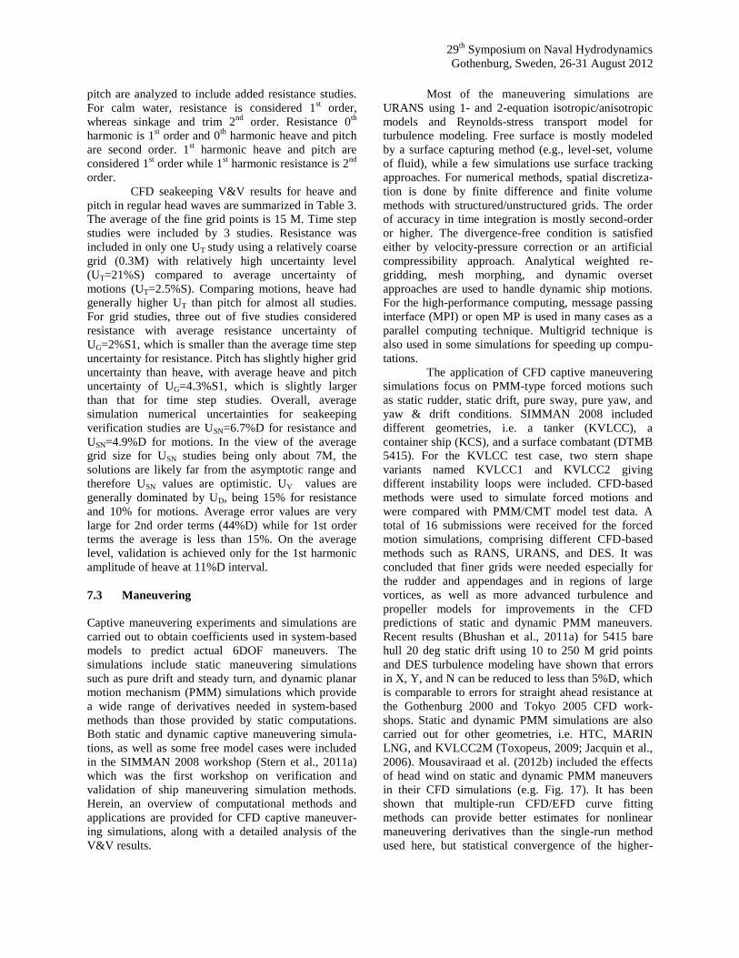
29th
Symposium on Naval Hydrodynamics
Gothenburg, Sweden, 26-31 August 2012
pitch are analyzed to include added resistance studies.
For calm water, resistance is considered 1st order,
whereas sinkage and trim 2nd
order. Resistance 0th
harmonic is 1st order and 0
th harmonic heave and pitch
are second order. 1st harmonic heave and pitch are
considered 1st order while 1
st harmonic resistance is 2
nd
order.
CFD seakeeping V&V results for heave and
pitch in regular head waves are summarized in Table 3.
The average of the fine grid points is 15 M. Time step
studies were included by 3 studies. Resistance was
included in only one UT study using a relatively coarse
grid (0.3M) with relatively high uncertainty level
(UT=21%S) compared to average uncertainty of
motions (UT=2.5%S). Comparing motions, heave had
generally higher UT than pitch for almost all studies.
For grid studies, three out of five studies considered
resistance with average resistance uncertainty of
UG=2%S1, which is smaller than the average time step
uncertainty for resistance. Pitch has slightly higher grid
uncertainty than heave, with average heave and pitch
uncertainty of UG=4.3%S1, which is slightly larger
than that for time step studies. Overall, average
simulation numerical uncertainties for seakeeping
verification studies are USN=6.7%D for resistance and
USN=4.9%D for motions. In the view of the average
grid size for USN studies being only about 7M, the
solutions are likely far from the asymptotic range and
therefore USN values are optimistic. UV values are
generally dominated by UD, being 15% for resistance
and 10% for motions. Average error values are very
large for 2nd order terms (44%D) while for 1st order
terms the average is less than 15%. On the average
level, validation is achieved only for the 1st harmonic
amplitude of heave at 11%D interval.
7.3 Maneuvering
Captive maneuvering experiments and simulations are
carried out to obtain coefficients used in system-based
models to predict actual 6DOF maneuvers. The
simulations include static maneuvering simulations
such as pure drift and steady turn, and dynamic planar
motion mechanism (PMM) simulations which provide
a wide range of derivatives needed in system-based
methods than those provided by static computations.
Both static and dynamic captive maneuvering simula-
tions, as well as some free model cases were included
in the SIMMAN 2008 workshop (Stern et al., 2011a)
which was the first workshop on verification and
validation of ship maneuvering simulation methods.
Herein, an overview of computational methods and
applications are provided for CFD captive maneuver-
ing simulations, along with a detailed analysis of the
V&V results.
Most of the maneuvering simulations are
URANS using 1- and 2-equation isotropic/anisotropic
models and Reynolds-stress transport model for
turbulence modeling. Free surface is mostly modeled
by a surface capturing method (e.g., level-set, volume
of fluid), while a few simulations use surface tracking
approaches. For numerical methods, spatial discretiza-
tion is done by finite difference and finite volume
methods with structured/unstructured grids. The order
of accuracy in time integration is mostly second-order
or higher. The divergence-free condition is satisfied
either by velocity-pressure correction or an artificial
compressibility approach. Analytical weighted re-
gridding, mesh morphing, and dynamic overset
approaches are used to handle dynamic ship motions.
For the high-performance computing, message passing
interface (MPI) or open MP is used in many cases as a
parallel computing technique. Multigrid technique is
also used in some simulations for speeding up compu-
tations.
The application of CFD captive maneuvering
simulations focus on PMM-type forced motions such
as static rudder, static drift, pure sway, pure yaw, and
yaw & drift conditions. SIMMAN 2008 included
different geometries, i.e. a tanker (KVLCC), a
container ship (KCS), and a surface combatant (DTMB
5415). For the KVLCC test case, two stern shape
variants named KVLCC1 and KVLCC2 giving
different instability loops were included. CFD-based
methods were used to simulate forced motions and
were compared with PMM/CMT model test data. A
total of 16 submissions were received for the forced
motion simulations, comprising different CFD-based
methods such as RANS, URANS, and DES. It was
concluded that finer grids were needed especially for
the rudder and appendages and in regions of large
vortices, as well as more advanced turbulence and
propeller models for improvements in the CFD
predictions of static and dynamic PMM maneuvers.
Recent results (Bhushan et al., 2011a) for 5415 bare
hull 20 deg static drift using 10 to 250 M grid points
and DES turbulence modeling have shown that errors
in X, Y, and N can be reduced to less than 5%D, which
is comparable to errors for straight ahead resistance at
the Gothenburg 2000 and Tokyo 2005 CFD work-
shops. Static and dynamic PMM simulations are also
carried out for other geometries, i.e. HTC, MARIN
LNG, and KVLCC2M (Toxopeus, 2009; Jacquin et al.,
2006). Mousaviraad et al. (2012b) included the effects
of head wind on static and dynamic PMM maneuvers
in their CFD simulations (e.g. Fig. 17). It has been
shown that multiple-run CFD/EFD curve fitting
methods can provide better estimates for nonlinear
maneuvering derivatives than the single-run method
used here, but statistical convergence of the higher-
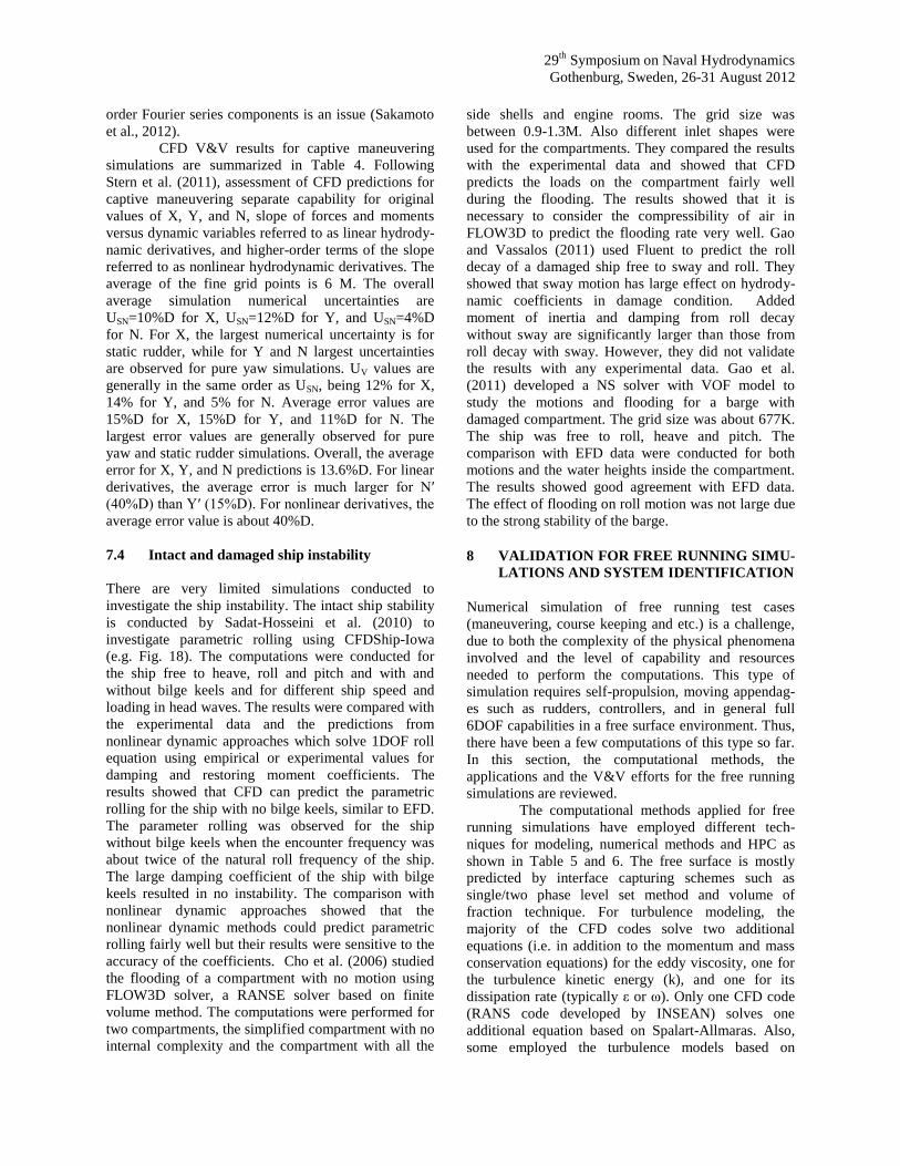
29th
Symposium on Naval Hydrodynamics
Gothenburg, Sweden, 26-31 August 2012
order Fourier series components is an issue (Sakamoto
et al., 2012).
CFD V&V results for captive maneuvering
simulations are summarized in Table 4. Following
Stern et al. (2011), assessment of CFD predictions for
captive maneuvering separate capability for original
values of X, Y, and N, slope of forces and moments
versus dynamic variables referred to as linear hydrody-
namic derivatives, and higher-order terms of the slope
referred to as nonlinear hydrodynamic derivatives. The
average of the fine grid points is 6 M. The overall
average simulation numerical uncertainties are
USN=10%D for X, USN=12%D for Y, and USN=4%D
for N. For X, the largest numerical uncertainty is for
static rudder, while for Y and N largest uncertainties
are observed for pure yaw simulations. UV values are
generally in the same order as USN, being 12% for X,
14% for Y, and 5% for N. Average error values are
15%D for X, 15%D for Y, and 11%D for N. The
largest error values are generally observed for pure
yaw and static rudder simulations. Overall, the average
error for X, Y, and N predictions is 13.6%D. For linear
derivatives, the average error is much larger for Nʹ
(40%D) than Yʹ (15%D). For nonlinear derivatives, the
average error value is about 40%D.
7.4 Intact and damaged ship instability
There are very limited simulations conducted to
investigate the ship instability. The intact ship stability
is conducted by Sadat-Hosseini et al. (2010) to
investigate parametric rolling using CFDShip-Iowa
(e.g. Fig. 18). The computations were conducted for
the ship free to heave, roll and pitch and with and
without bilge keels and for different ship speed and
loading in head waves. The results were compared with
the experimental data and the predictions from
nonlinear dynamic approaches which solve 1DOF roll
equation using empirical or experimental values for
damping and restoring moment coefficients. The
results showed that CFD can predict the parametric
rolling for the ship with no bilge keels, similar to EFD.
The parameter rolling was observed for the ship
without bilge keels when the encounter frequency was
about twice of the natural roll frequency of the ship.
The large damping coefficient of the ship with bilge
keels resulted in no instability. The comparison with
nonlinear dynamic approaches showed that the
nonlinear dynamic methods could predict parametric
rolling fairly well but their results were sensitive to the
accuracy of the coefficients. Cho et al. (2006) studied
the flooding of a compartment with no motion using
FLOW3D solver, a RANSE solver based on finite
volume method. The computations were performed for
two compartments, the simplified compartment with no
internal complexity and the compartment with all the
side shells and engine rooms. The grid size was
between 0.9-1.3M. Also different inlet shapes were
used for the compartments. They compared the results
with the experimental data and showed that CFD
predicts the loads on the compartment fairly well
during the flooding. The results showed that it is
necessary to consider the compressibility of air in
FLOW3D to predict the flooding rate very well. Gao
and Vassalos (2011) used Fluent to predict the roll
decay of a damaged ship free to sway and roll. They
showed that sway motion has large effect on hydrody-
namic coefficients in damage condition. Added
moment of inertia and damping from roll decay
without sway are significantly larger than those from
roll decay with sway. However, they did not validate
the results with any experimental data. Gao et al.
(2011) developed a NS solver with VOF model to
study the motions and flooding for a barge with
damaged compartment. The grid size was about 677K.
The ship was free to roll, heave and pitch. The
comparison with EFD data were conducted for both
motions and the water heights inside the compartment.
The results showed good agreement with EFD data.
The effect of flooding on roll motion was not large due
to the strong stability of the barge.
8 VALIDATION FOR FREE RUNNING SIMU-
LATIONS AND SYSTEM IDENTIFICATION
Numerical simulation of free running test cases
(maneuvering, course keeping and etc.) is a challenge,
due to both the complexity of the physical phenomena
involved and the level of capability and resources
needed to perform the computations. This type of
simulation requires self-propulsion, moving appendag-
es such as rudders, controllers, and in general full
6DOF capabilities in a free surface environment. Thus,
there have been a few computations of this type so far.
In this section, the computational methods, the
applications and the V&V efforts for the free running
simulations are reviewed.
The computational methods applied for free
running simulations have employed different tech-
niques for modeling, numerical methods and HPC as
shown in Table 5 and 6. The free surface is mostly
predicted by interface capturing schemes such as
single/two phase level set method and volume of
fraction technique. For turbulence modeling, the
majority of the CFD codes solve two additional
equations (i.e. in addition to the momentum and mass
conservation equations) for the eddy viscosity, one for
the turbulence kinetic energy (k), and one for its
dissipation rate (typically ε or ω). Only one CFD code
(RANS code developed by INSEAN) solves one
additional equation based on Spalart-Allmaras. Also,
some employed the turbulence models based on
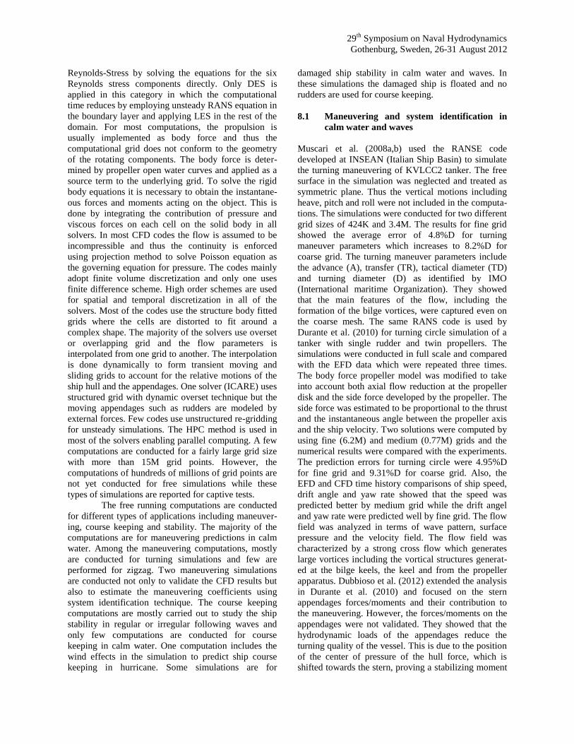
29th
Symposium on Naval Hydrodynamics
Gothenburg, Sweden, 26-31 August 2012
Reynolds-Stress by solving the equations for the six
Reynolds stress components directly. Only DES is
applied in this category in which the computational
time reduces by employing unsteady RANS equation in
the boundary layer and applying LES in the rest of the
domain. For most computations, the propulsion is
usually implemented as body force and thus the
computational grid does not conform to the geometry
of the rotating components. The body force is deter-
mined by propeller open water curves and applied as a
source term to the underlying grid. To solve the rigid
body equations it is necessary to obtain the instantane-
ous forces and moments acting on the object. This is
done by integrating the contribution of pressure and
viscous forces on each cell on the solid body in all
solvers. In most CFD codes the flow is assumed to be
incompressible and thus the continuity is enforced
using projection method to solve Poisson equation as
the governing equation for pressure. The codes mainly
adopt finite volume discretization and only one uses
finite difference scheme. High order schemes are used
for spatial and temporal discretization in all of the
solvers. Most of the codes use the structure body fitted
grids where the cells are distorted to fit around a
complex shape. The majority of the solvers use overset
or overlapping grid and the flow parameters is
interpolated from one grid to another. The interpolation
is done dynamically to form transient moving and
sliding grids to account for the relative motions of the
ship hull and the appendages. One solver (ICARE) uses
structured grid with dynamic overset technique but the
moving appendages such as rudders are modeled by
external forces. Few codes use unstructured re-gridding
for unsteady simulations. The HPC method is used in
most of the solvers enabling parallel computing. A few
computations are conducted for a fairly large grid size
with more than 15M grid points. However, the
computations of hundreds of millions of grid points are
not yet conducted for free simulations while these
types of simulations are reported for captive tests.
The free running computations are conducted
for different types of applications including maneuver-
ing, course keeping and stability. The majority of the
computations are for maneuvering predictions in calm
water. Among the maneuvering computations, mostly
are conducted for turning simulations and few are
performed for zigzag. Two maneuvering simulations
are conducted not only to validate the CFD results but
also to estimate the maneuvering coefficients using
system identification technique. The course keeping
computations are mostly carried out to study the ship
stability in regular or irregular following waves and
only few computations are conducted for course
keeping in calm water. One computation includes the
wind effects in the simulation to predict ship course
keeping in hurricane. Some simulations are for
damaged ship stability in calm water and waves. In
these simulations the damaged ship is floated and no
rudders are used for course keeping.
8.1 Maneuvering and system identification in
calm water and waves
Muscari et al. (2008a,b) used the RANSE code
developed at INSEAN (Italian Ship Basin) to simulate
the turning maneuvering of KVLCC2 tanker. The free
surface in the simulation was neglected and treated as
symmetric plane. Thus the vertical motions including
heave, pitch and roll were not included in the computa-
tions. The simulations were conducted for two different
grid sizes of 424K and 3.4M. The results for fine grid
showed the average error of 4.8%D for turning
maneuver parameters which increases to 8.2%D for
coarse grid. The turning maneuver parameters include
the advance (A), transfer (TR), tactical diameter (TD)
and turning diameter (D) as identified by IMO
(International maritime Organization). They showed
that the main features of the flow, including the
formation of the bilge vortices, were captured even on
the coarse mesh. The same RANS code is used by
Durante et al. (2010) for turning circle simulation of a
tanker with single rudder and twin propellers. The
simulations were conducted in full scale and compared
with the EFD data which were repeated three times.
The body force propeller model was modified to take
into account both axial flow reduction at the propeller
disk and the side force developed by the propeller. The
side force was estimated to be proportional to the thrust
and the instantaneous angle between the propeller axis
and the ship velocity. Two solutions were computed by
using fine (6.2M) and medium (0.77M) grids and the
numerical results were compared with the experiments.
The prediction errors for turning circle were 4.95%D
for fine grid and 9.31%D for coarse grid. Also, the
EFD and CFD time history comparisons of ship speed,
drift angle and yaw rate showed that the speed was
predicted better by medium grid while the drift angel
and yaw rate were predicted well by fine grid. The flow
field was analyzed in terms of wave pattern, surface
pressure and the velocity field. The flow field was
characterized by a strong cross flow which generates
large vortices including the vortical structures generat-
ed at the bilge keels, the keel and from the propeller
apparatus. Dubbioso et al. (2012) extended the analysis
in Durante et al. (2010) and focused on the stern
appendages forces/moments and their contribution to
the maneuvering. However, the forces/moments on the
appendages were not validated. They showed that the
hydrodynamic loads of the appendages reduce the
turning quality of the vessel. This is due to the position
of the center of pressure of the hull force, which is
shifted towards the stern, proving a stabilizing moment
29th
Symposium on Naval Hydrodynamics
Gothenburg, Sweden, 26-31 August 2012
which counteracts the vessel motion. It was also shown
that the appendages on the external side of turning
develop a higher lateral force with respect to the inner
side ones as the appendages in inner side are in wake of
the hull. Even though the lateral force of inner side
appendages were small, the induced moment was in the
same order as that developed by the bare hull. This
stresses the extreme importance of the stern appendag-
es on the maneuvering behavior of the vessels.
Jacquin et al. (2006) employed ICARE, the
RANS code developed by ECN (Ecole Centrale de
Nantes) in France. They performed turning maneuver
of a containership (Series 60). They mentioned that the
computations were conducted with actual moving
rudders and also with simplified condition where a side
force was used to mimic the existence of a deflected
rudder behind the ship. However, only the free running
results of the model with side force were reported. The
computations were only conducted to demonstrate the
capability of ICARE in free running maneuvering and
no validations were shown. The solver ICARE later
was used by Ferrant et al. (2008) and Drouet et al.
(2008). Ferrant et al. (2008) demonstrated the capabil-
ity of ICARE for turning circle simulation in regular
waves for 5415M, a surface combatant. The rudder was
approximated by a time varying side force applied at
the rudder location. The Wave is treated using
SWENSE (Spectral Wave Explicit Navier-Stokes
Equations) approach by combining the description of
undisturbed incident waves introduced by a non-linear
spectral scheme in potential flow theory and the
computation of the non-linear viscous diffracted flow
using the free surface RANS solver. Since there is no
direct impose of wave condition on free surface, there
would be no need to have a fine grid to ensure a good
propagation of the waves. Drouet et al. (2008) con-
ducted turning maneuver simulations for Humburg test
case and 5415M using ICARE solver. For both
geometries, the rudders were modeled by an external
side force. For Humburg test case, the simulations were
conducted for the model free to horizontal motions
(surge, sway and yaw) and also free to all motions. The
comparison with EFD data showed better agreement
for 3DOF simulations with error of 0.3%D for tactical
diameter compared to 5%D for free simulations. For
5415M, the turning maneuver results were reported in
calm water and waves but no validation was conducted.
For calm water, a model with different bulb forms were
considered and showed that the tactical diameter
reduces 5% for a bulb form shorter and more immerged
than the initial form.
Carrica et al. (2008a) employed CFDShip-
Iowa for turning and zigzag maneuver simulations in
calm water and waves for 5415M. The body force
propeller model was used for the propulsion and the
actual rudders were included in the simulations. The
results were obtained using both constant propeller rate
and constant torque condition for propellers. The total
grid points were 7M for calm water increasing to 12M
for waves. The simulations were conducted for both
model and full scale and no validation was reported.
The details of turbulence modeling for the model scale
and full scale simulations were discussed later in
Bhushan et al. (2009). For model scale simulations,
blended k-w was used while for full scale computations
the multilayer wall-function models were employed.
For zigzag simulations, the full scale case reached the
rudder check points faster than that of model scale,
indicating a slightly more efficient rudder action in full
scale. Since the boundary layer was thicker in the
model scale case, the lower velocities at the propeller
plane was expected compared to that of full scale. This
provided higher velocity reaching the rudders for full
scale and consequently better steering capacity. For
turning simulations in waves, with constant RPM, the
ship was locked in the wave when the wave was
following waves providing surf-riding. In the case of
constant torque the ship did not have enough power
and the following waves could overcome the ship. The
validation of calm water turning and zigzag simulations
for 5415M was reported in Carrica et al. (2012b).
Figure 19 shows the predicted free surface and vortical
structures during turning circle reported in Carrica et
al. (2012b). The average error of turning and zigzag
maneuvers predictions were 5.74%D and 6.83%D,
respectively. Mousaviraad et al. (2012a) used CFD-
Ship-Iowa for turning and zigzag maneuvering of a
surface effect ship (SES), as shown in Figure 20. The
body force propeller model was used in the simulation.
The simulations were conducted in both deep and
shallow water and in both calm water and waves with
the grid size of 8.6-9.3M. It was shown that shallow
water increases transfer and tactical diameter in turning
maneuvers. However, radius and yaw rate showed no
change in shallow and deep water. Also, shallow water
reduced the 1st and 2nd overshoot for zigzag. For
turning, wave effect is significant on the maneuver of
the ship in shallow water. For zigzag, the waves reduce
the overshoot angle. Sadat-Hosseini et al. (2011a) and
Araki et al. (2012a, b) employed CFDShip-Iowa for a
surface combatant (ONR Tumblehome) maneuvering
in calm water and waves. The model included all the
appendages with grid size of 12.1M in total but the
propellers were simulated using body force. The
average error for calm water simulations were 1.62%D
and 1.88%D for turning and zigzag. The results for
waves also showed very good agreement with the EFD
data. They also used system identification technique
for first time to improve the maneuvering coefficients
and their variations induced by waves, rudder forces
and wave forces from CFD free running outputs. They
used two system identification methods including
29th
Symposium on Naval Hydrodynamics
Gothenburg, Sweden, 26-31 August 2012
extended Kalman filter (EKF) and constrained least
square (CLS). The results in calm water showed the
average system based prediction errors for maneuver-
ing simulations drop from 16% to 8% by using the
maneuvering coefficients and rudder forces found from
CFD free running instead of those from captive
experiments (see Figure 21). Also, the system based
results in waves were significantly improved by tuning
the maneuvering coefficients and wave forces in the
mathematical model using CFD outputs.
8.2 Course keeping and stability in calm water
and waves
Carrica et al. (2008b) and Huang et al. (2008) demon-
strated the capability of CFDShip-Iowa for course
keeping and the instability of ONR Tumblehome in
irregular following waves. The actual rudder was
included in the simulation and the propeller was
modeled through a body force. Broaching was
predicted during the course keeping but the results
were not validated. Mousaviraad et al. (2008) demon-
strated the capability of CFDShip-Iowa for course
keeping in waves in present of significant winds. They
simulated course keeping in CAMILLE hurricane for
ship in quartering waves with winds hitting the ship at
45 and 225 deg. The results showed the wind has
strong effects on ship forces and moments. The case
with wind from 45 deg loses control at some instants
but regains control while the ship turns to port and
cannot be controlled for the case with wind at 225 deg.
Sadat-Hosseini et al. (2011b) validated the course
keeping and instability of ONR Tumblehome for
various speed and heading in regular following waves.
The CFD simulation could remarkably predict the
instability map. CFD predicted the boundary between
periodic motion and surf-riding/broaching at Fr=0.3 for
heading less than 30 degrees. Periodic motion was
predicted below the boundary (Fr<0.3) whereas surf-
riding/broaching was observed above the boundary, in
agreement with EFD. However, there were discrepan-
cies in the time histories due to missing EFD initial
condition for ship speed and wave phase. The authors
later included the actual propeller in the simulation and
showed improvement for the time histories of all
motions (Carrica et al., 2012a). Also direct integration
of forces and moments on all appendages were
conducted to investigate the contribution of the
appendages on the instability of the ship during the
course keeping. The yaw moments showed that the
turning moments produced by the appendages were
dominated by the rudders, with values one order of
magnitude larger than any other appendage. Also, both
propellers contributed a net positive turning, helping
prevent broaching. The CFD solutions for broaching
using both body force and actual propeller are shown in
Figures. 22 a and b.
The validation of forces and moments on the
appendages in free running simulations were per-
formed by Stern et al. (2011b) and Sadat-Hosseini et al.
(2012a). They employed CFDShip-Iowa and ISIS-CFD
to study the predictions of course keeping for 5415M in
calm water and regular waves. The CFDShip-Iowa
simulations included course keeping under either roll
decay or forced roll in calm water and course keeping
in head and beam waves. For ISIS-CFD computations,
the roll decay in calm water was only performed. The
moving rudders and stabilizers were included in
CFDShip-Iowa while both were fixed in ISIS-CFD.
The propeller was modeled as a body force in both
solvers. The grid size for CFDShip-Iowa and ISIS-
CFD was 6.3-18.6M and 5.9M, respectively. The
results showed very good agreement with EFD data
using both CFD simulations. Also, the CFD results
were compared with potential flow and system based
method predictions and confirmed that CFD provides
better results than the other methods. Figure 23 shows
the grid topology and the instant view of CFDShip-
Iowa solution during course keeping in beam waves.
Sadat-Hosseini et al. (2012b) extended the validation
of forces and moments to irregular wave condition, as
shown in Figure 24. The irregular wave was generated
by summation of many regular waves with amplitudes
computed from the desired wave spectrum and with
random phases. A very fine grid was used to resolve all
the components of the irregular waves from very small
to very large amplitudes. The grid size was about 24M,
decomposed into 249 CPUs for parallel processing.
The computations were conducted for course keeping
of a surface combatant in irregular beam waves for
JONSWAP wave spectrum and the results were
compared with the experimental data. The results were
validated against the experiments not only for the ship
motions but also for the loads on the appendages. The
correlation between ship motions and input irregular
waves were also studied. Comparing the irregular wave
results with the results computed from regular wave
simulations at several discrete wave length conditions
showed that the ship has fairly similar motion in both
regular and irregular waves with same wave length
condition.
Dreyer and Boger (2010) used OVER-
REL_TCURS solver to simulate the overtaking of a
submarine and a ship. The OVER-REL_TCURS solver
is developed at ARL (Applied Research Laboratory,
Pennsylvania State University). The free surface is
ignored in the simulation. The body force propeller
model was used in the simulation for both the ship and
the submarine. The grid size of the ship and submarine
was 2.3M and 4.1M, respectively. The comparisons
were performed for depth and pitch. Good agreement
29th
Symposium on Naval Hydrodynamics
Gothenburg, Sweden, 26-31 August 2012
with EFD was obtained for locked fin cases but large
discrepancies for those cases with moving fins were
observed. A few simulations were conducted for the
ship with damaged compartment to investigate the
stability of the ship under damaged condition.
Strasser et al. (2009) conducted CFD simula-
tion of floating damaged barge. They included the
compressibility of the air trapped in the damaged
compartment. The time histories of sinkage, trim, heel
and water height inside the compartment were
compared with EFD data and the results showed very
good agreement. Sadat-Hosseini et al. (2012c)
employed CFDShip-Iowa for a damaged ship and
investigated roll decay and motions with flooding in
calm water and waves. The grid size was in range of
6.3-28M, depending on the case. The results were
compared with experimental data not only for ship
motions but also for the water height inside the
compartment to evaluate the flooding rate prediction.
The verification study was also conducted, showing
that the results were not very sensitive to the numerical
uncertainty. Overall CFD showed good agreement with
experimental results for both ship motions and water
heights inside the compartment for all cases in calm
water and waves. CFD results could capture the
complex free surface shape inside the compartment
generated by the flooded water and the reflected water
by the walls inside the compartment (see Figure 25).
For roll decay cases, CFD showed that the damping
coefficient is larger and roll frequency is smaller for
the roll decay under damaged condition.
9 FUNDAMENTAL STUDIES FOR TWO-
PHASE FLOWS
Breaking waves, spray formation, and air entrainment
around ships are one of the main sources of the
underwater sounds and white-water wakes, which are
of great importance for signature of ships. These flow
phenomena occur on a large range of temporal and
spatial scales. At small scales, spray formation and air
entrainment in the contact line region depend on the
length scales which are orders of magnitude smaller
than the length of the ship with correspondingly small
time scale. For the large scales, the overall structures
include wave breakings along the hull and the induced
vortices, instabilities, separations and scars, etc.
Understanding the small scale physics and capturing
their effects on the large scale features are of primary
importance for ship hydrodynamics. Skin-friction drag
reduction is of great significance in ship hydrodynam-
ics. One of the important techniques for the drag
reduction is to inject gas into the liquid turbulent
boundary layer to form bubbles or air layer. In this
section, fundamental studies for two-phase flows in
ship hydrodynamics are reviewed.
9.1 Flow around surface-piercing object
Experimental and computational studies have been
conducted for the flows of a surface-piercing flat plate
with focus on the wave induced effects on the flat plate
boundary layer below the juncture region (Stern, 1986;
Stern et al., 1989; Stern et al., 1993). More recent
experimental and computational studies focused on the
juncture region and turbulence modeling using towed,
two-dimensional laser-doppler velocimetry (LDV) and
RANS and large-eddy simulation (LES) methods for
flat free surface (Longo et al., 1998; Sreedhar and
Stern, 1998a, b). The juncture region experiment
(Longo et al.,1998) is extended to include wave effects
using servomechanism wave gauges (Kang et al.,
2008). It is observed that the interface appears always
broken in the contact line region even for the case with
a smooth wave field. Air is entrained into the boundary
layer at the contact line region due to the interaction of
the contact line with the solid surface. A string of
bubbles can be generated near the solid wall usually
with small bubble sizes. For flows past a blunt leading
edge, such as NACA0024 foil, the bow wave breaks
and wraps around the bow with similar features to
spilling breakers (Metcalf et al., 2006) at a Fr number
of 0.37. Wave induced flow separation occurs and
reattaches to the foil surface resulting in a wall-
bounded separation bubble. The complexity of
unsteady, wave-induced, boundary layer separation
makes the experimental measurements difficult. With
the combined CFD studies (Kandasamy et al., 2009
and Xing et al., 2007), more detailed flow description
is provided. Three main instabilities, namely the initial
shear-layer instability, Karman-like shedding and
flapping of the separation bubble, were found in the
unsteady Reynolds-averaged Navier-Stokes (URANS)
study (Kandasamy et al., 2009). These instabilities are
difficult to be identified in both the DES study (Xing et
al., 2007) and experimental study (Metcalf et al., 2006)
due to the numerous small-scale vortices in the
separation region. There are limitations in both of the
two CFD studies. The complicated flow structures at
the interface as shown in the experimental images, such
as splashing, breaking waves, air entrainment and free
surface induced turbulence observed in the experi-
ments, cannot be resolved since a single phase flow
solver (air effect is neglected) and relatively less
accurate interface modeling methods were used. These
unresolved flow structures at the interface might affect
the global flow patterns and turbulence. In Suh et al.
(2011), flows past an interface piercing circular
cylinder is investigated using LES with a focus on the
effect of air–water interface on the vortex shedding
from the vertical circular cylinder (selected results
shown in Fig. 26).
29th
Symposium on Naval Hydrodynamics
Gothenburg, Sweden, 26-31 August 2012
Previous studies are mainly focused on the
global structure of ship flows, such as the wave
elevation, scars, and vortices. The small scale details of
interface breaking, spray formation, and air entrain-
ment are not well understood.
9.2 Bow wave breaking and spray formation
Ship bow waves exhibit both large and small scale
features. The most prominent large scale feature is the
Kelvin bow wave pattern scaled by Fr; however, for
sufficiently large Fr and depending on bow shape,
spilling and/or plunging breaking occurs and induces
vortices and scars additionally scaled by Re and We.
Small Re and We inhibit breaking, i.e., in general
model scale flows exhibit reduced breaking compared
to full scale, and smaller models display reduced
breaking compared to larger models. A recent com-
plementary EFD and CFD study has documented bow
wave breaking and induced vortices and scars for
model 5415 for Fr = 0.35 using CFDShip-Iowa Version
4 (Olivieri et al., 2007; Wilson et al., 2007a). The most
prominent small scale feature is the bow wave crest
formation of thin overturning sheets which break up
into spray. In the study by Beale et al. (2010), recent
in-situ measurement efforts were reviewed and spray
formation generated by full-scale naval platforms were
examined. Re and We scale effects are large such that
replication of full scale phenomena of the small scale
features of ship bow waves is difficult even with large
models. The extent of the thin sheets is drastically
reduced and remains attached, as shown by Stern et al.
(1996) for the Series 60.
However, studies for wedge flows by
Waniewski et al. (2002) and Karion et al. (2004)
display and document the structure of bow waves (thin
water sheet formation, overturning sheet with surface
disturbance, fingering and breaking up into spray,
plunging and splashing, and air entrainment) with
valuable experimental data provided such as wave
elevation, extent of wave breaking, spray droplets size
and number. These two studies are summarized in
Table 7. In Waniewski et al. (2002) the bow waves are
created by a deflecting plate mounted at an angle in a
flume, the towing tank experiments are also conducted
with two wedge models. Typical bow wave profile
obtained in the towing tank experiment shows a thin
liquid sheet is created at the leading edge of the wedge,
and it continues to ride up on the side wall. This thin
liquid sheet starts to separate from the side wall as it
reaches its maximum height. Once the crest reaches its
maximum height, an overturning jet is formed and
plunges back onto the undisturbed free surface. A large
area of splash is generated at the wake of the wedge
due to wave plunge and air entrainment. Noblesse et al.
(2008) proposed a series of simple analytical relations
for a wedge-shaped bow wave based on the experi-
mental measurements and elementary fundamental
considerations, which define the main characteristics of
a ship bow (wave height, wave crest location and
profile, and flow steadiness or unsteadiness) in terms of
ship speed U, draught D and waterline entrance angle
2θ. A computational study has been carried out by
Broglia et al. (2004) with the results compared with the
experimental data (Waniewski et al., 2002). Since a
single phase level set method was used for the free
surface tracking, the small scale interface structures
were not captured. The mechanism of the liquid sheet
disturbance, fingering, pinching off drops and spray
formation has not been thoroughly studied.
In Wang et al. (2010b), flows around a wedge-
shaped bow are numerically simulated with the aim of
investigating the wave breaking mechanism and small
scale features of ship bow waves. The study (Waniew-
ski et al., 2002) was selected as test cases to validate
the capability of the code of CFDShip-Iowa Version 6
(Yang and Stern, 2009; Wang et al., 2009b) for small
scale features of ship bow waves. The simulations are
carried out using a Cartesian grid solver first with the
sharp interface, coupled level set and volume-of-fluid
(CLSVOF) and immersed boundaries methods; and an
orthogonal curvilinear grid solver (Wang et al., 2012a)
is also used in order to increase the grid resolutions
near the wall.
The wedge geometry is similar to the large
wedge model used by Waniewski et al. (2002). The
side length of the wedge is L = 0.75 m, and the height
of the wedge is H = 1 m. The half wedge angle is θ =
26º and the flare angle φ = 0º. The sharp edge corners
are rounded with an arc of a small radius in order to
make the grid orthogonal at the two corners. The grid is
1536×768×848 (one billion) which is refined near the
solid surface.
For the case considered here, the water depth
is d = 0.0745 m and the upstream velocity is U = 2.5
m/s, the corresponding Reynolds number,
/Re Ud = 1.64×10⁵, and the Froude number,
gdUFr / = 2.93. The domain boundary is given
by x = [5.33 m, 4.55 m], y = [0.0745 m, 0.6 m], and z =
[0 m, 5 m]. Uniform inflow and convective outflow
boundary conditions are used. Slip-wall boundary
conditions are imposed at all the other boundaries. A
uniform velocity field same as the upstream velocity is
prescribed to the entire computational domain at t = 0.
Figure 27 shows the computed bow wave profile
compared with the experimental video image. The
overall wave structure is very similar to the experi-
mental observation (Waniewski et al., 2002) as shown
in figure, such as the thin liquid sheet at the leading
edge of the bow, overturning jet, jet plunging onto the
free surface, and splashes at the wake. As the liquid
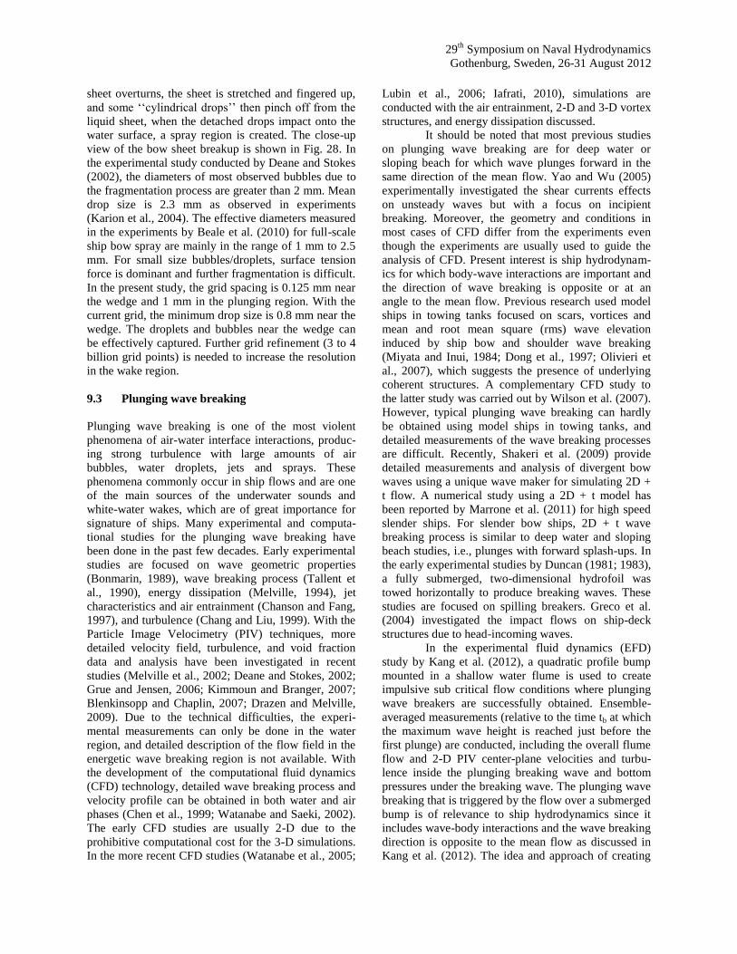
29th
Symposium on Naval Hydrodynamics
Gothenburg, Sweden, 26-31 August 2012
sheet overturns, the sheet is stretched and fingered up,
and some ‘‘cylindrical drops’’ then pinch off from the
liquid sheet, when the detached drops impact onto the
water surface, a spray region is created. The close-up
view of the bow sheet breakup is shown in Fig. 28. In
the experimental study conducted by Deane and Stokes
(2002), the diameters of most observed bubbles due to
the fragmentation process are greater than 2 mm. Mean
drop size is 2.3 mm as observed in experiments
(Karion et al., 2004). The effective diameters measured
in the experiments by Beale et al. (2010) for full-scale
ship bow spray are mainly in the range of 1 mm to 2.5
mm. For small size bubbles/droplets, surface tension
force is dominant and further fragmentation is difficult.
In the present study, the grid spacing is 0.125 mm near
the wedge and 1 mm in the plunging region. With the
current grid, the minimum drop size is 0.8 mm near the
wedge. The droplets and bubbles near the wedge can
be effectively captured. Further grid refinement (3 to 4
billion grid points) is needed to increase the resolution
in the wake region.
9.3 Plunging wave breaking
Plunging wave breaking is one of the most violent
phenomena of air-water interface interactions, produc-
ing strong turbulence with large amounts of air
bubbles, water droplets, jets and sprays. These
phenomena commonly occur in ship flows and are one
of the main sources of the underwater sounds and
white-water wakes, which are of great importance for
signature of ships. Many experimental and computa-
tional studies for the plunging wave breaking have
been done in the past few decades. Early experimental
studies are focused on wave geometric properties
(Bonmarin, 1989), wave breaking process (Tallent et
al., 1990), energy dissipation (Melville, 1994), jet
characteristics and air entrainment (Chanson and Fang,
1997), and turbulence (Chang and Liu, 1999). With the
Particle Image Velocimetry (PIV) techniques, more
detailed velocity field, turbulence, and void fraction
data and analysis have been investigated in recent
studies (Melville et al., 2002; Deane and Stokes, 2002;
Grue and Jensen, 2006; Kimmoun and Branger, 2007;
Blenkinsopp and Chaplin, 2007; Drazen and Melville,
2009). Due to the technical difficulties, the experi-
mental measurements can only be done in the water
region, and detailed description of the flow field in the
energetic wave breaking region is not available. With
the development of the computational fluid dynamics
(CFD) technology, detailed wave breaking process and
velocity profile can be obtained in both water and air
phases (Chen et al., 1999; Watanabe and Saeki, 2002).
The early CFD studies are usually 2-D due to the
prohibitive computational cost for the 3-D simulations.
In the more recent CFD studies (Watanabe et al., 2005;
Lubin et al., 2006; Iafrati, 2010), simulations are
conducted with the air entrainment, 2-D and 3-D vortex
structures, and energy dissipation discussed.
It should be noted that most previous studies
on plunging wave breaking are for deep water or
sloping beach for which wave plunges forward in the
same direction of the mean flow. Yao and Wu (2005)
experimentally investigated the shear currents effects
on unsteady waves but with a focus on incipient
breaking. Moreover, the geometry and conditions in
most cases of CFD differ from the experiments even
though the experiments are usually used to guide the
analysis of CFD. Present interest is ship hydrodynam-
ics for which body-wave interactions are important and
the direction of wave breaking is opposite or at an
angle to the mean flow. Previous research used model
ships in towing tanks focused on scars, vortices and
mean and root mean square (rms) wave elevation
induced by ship bow and shoulder wave breaking
(Miyata and Inui, 1984; Dong et al., 1997; Olivieri et
al., 2007), which suggests the presence of underlying
coherent structures. A complementary CFD study to
the latter study was carried out by Wilson et al. (2007).
However, typical plunging wave breaking can hardly
be obtained using model ships in towing tanks, and
detailed measurements of the wave breaking processes
are difficult. Recently, Shakeri et al. (2009) provide
detailed measurements and analysis of divergent bow
waves using a unique wave maker for simulating 2D +
t flow. A numerical study using a 2D + t model has
been reported by Marrone et al. (2011) for high speed
slender ships. For slender bow ships, 2D + t wave
breaking process is similar to deep water and sloping
beach studies, i.e., plunges with forward splash-ups. In
the early experimental studies by Duncan (1981; 1983),
a fully submerged, two-dimensional hydrofoil was
towed horizontally to produce breaking waves. These
studies are focused on spilling breakers. Greco et al.
(2004) investigated the impact flows on ship-deck
structures due to head-incoming waves.
In the experimental fluid dynamics (EFD)
study by Kang et al. (2012), a quadratic profile bump
mounted in a shallow water flume is used to create
impulsive sub critical flow conditions where plunging
wave breakers are successfully obtained. Ensemble-
averaged measurements (relative to the time tb at which
the maximum wave height is reached just before the
first plunge) are conducted, including the overall flume
flow and 2-D PIV center-plane velocities and turbu-
lence inside the plunging breaking wave and bottom
pressures under the breaking wave. The plunging wave
breaking that is triggered by the flow over a submerged
bump is of relevance to ship hydrodynamics since it
includes wave-body interactions and the wave breaking
direction is opposite to the mean flow as discussed in
Kang et al. (2012). The idea and approach of creating

29th
Symposium on Naval Hydrodynamics
Gothenburg, Sweden, 26-31 August 2012
plunging wave breakers using a submerged bump is
obtained collectively from the previous experimental
(Cahouet, 1984; Miyata et al., 1985a) and CFD studies
(Iafrati et al., 2001; Yang and Stern, 2007; Huang et
al., 2007). The CFD results were used as a guide for
the test design of the experiments (Ghosh, 2008) and
the initial experimental data was used for validation.
Subsequently, a complementary CFD study was used
to aid in the data analysis simultaneously as the
experimental data is used to validate a Cartesian grid,
immersed boundary, coupled level set and volume-of-
fluid CFD method (Wang et al., 2009b). Wang et al.
(2009b) indentified three repeated plunging events
each with three sub-events [jet impact (plunge),
oblique splash and vertical jet]; however, they used
fully impulsive initial conditions and adjusted the
initial velocity and water elevation to match Ghosh's
(2008) wave breaking position, which precluded
detailed temporal validation.
In the study by Koo et al. (2012), impulsive
plunging wave breaking downstream of a bump in a
shallow water flume is numerically simulated with the
aim of providing a detailed quantitative description of
the overall plunging wave breaking process. The time-
dependent velocity and wave elevation boundary
conditions are specified at the inlet and outlet using the
exact experimental data provided in Kang et al. (2012).
The computational results are compared with the
experimental measurements to validate the capability
of the code of CFDShip-Iowa Version 6 (Yang and
Stern, 2009; Wang et al., 2009b) for wave breaking.
The simulations are carried out on a 2D Cartesian grid
using the sharp interface, coupled level set and volume-
of-fluid (CLSVOF) and immersed boundary methods.
In the study by Wang et al. (2012b), a 3D LES of the
impulsive plunging wave breaking is performed on an
orthogonal curvilinear grid of 768×256×64 (stream-
wise, vertical, and spanwise) points in order to identify
the 3D structures of breaking interface. The constant
inlet velocity imposed at the left boundary is u = 0.87
m/s for water and zero for air. The initial interface
elevation is 0.2286 m and a uniform velocity field is
prescribed in the water domain with the air phase at
rest. The overall interface structure of the breaking
wave compared with the experimental video images is
given in Fig. 29. The major events of the first plunge
wave breaking are demonstrated, i.e., maximum height,
first plunge, oblique splash, and vertical jet as identi-
fied by Wang et al. (2009b) using 2D simulations. On
the video images, the entrapped air tube is marked by a
circle. As shown in the figure, the computational
results match the experiments very well. The 3D span-
wise interface structures due to the centrifugal
instabilities at the curved flow as observed in the
experiments are also captured as shown in Fig. 30.
In a 2D CFD study conducted by Iafrati
(2010) for Stokes waves, drops and bubbles in breaking
waves are quantitatively estimated with some limita-
tions due to the numerical model adopted in the
simulations. Recently, simulation on a large grid of
1920×1280×896 (2.2 billion) was carried out for
bubble/droplet size distribution in the breaking waves
(Wang et al., 2012d). Figure 31 shows the close-up of
the bubble and droplets in breaking waves on the large
grid, where detailed small interface structures are well
demonstrated.
9.4 Air-layer drag reduction
Bubble drag reduction (BDR) is an important technique
that injects gas into the liquid turbulent boundary layer
to form bubbles to obtain drag reduction. This tech-
nique can substantially reduce skin friction, which has
great potential applications in ship hydrodynamics.
During the past several decades, a large amount of
research has been devoted to the BDR (Merkle and
Deutsch, 1992). However, most of the studies were
conducted at relatively low Reynolds numbers and
small scales. Proper scaling of BDR remains unclear.
In the study by Sanders et al. (2006), a set of
BDR experiments were conducted for a large scale flat
plate turbulent boundary layer at high Reynolds
numbers. It has shown that significant levels of BDR
could be achieved only near the air injector, and
limited persistence of BDR exists away from the air
injector. This short persistence distance of BDR makes
it impractical for applications. It has also shown that a
layer of gas was formed and persisted along the entire
plate at lower flow speeds and higher gas injection
rates, which could lead to skin-friction reduction of
more than 80%. Elbing et al. (2008) continued the
study of Sanders et al. (2006) in an effort to understand
the mechanisms underlying the limited persistence of
the BDR and the onset conditions for the air layer drag
reduction (ALDR). The experimental results indicated
that ALDR could be established once the air was
injected beyond a critical rate, and more than 80% drag
reduction could be obtained over the entire plate. Three
distinct regions associated with drag reduction were
observed with air injection rate: BDR, transition and
ALDR. It was found that the air layer was sensitive to
the inflow conditions. In the recent work (Ceccio,
2009), a 1/2 inch (12.7 mm) step was used at the inlet,
and the air was injected from the base of the backward-
facing step. This greatly enhances the stability of the
air layer. The ALDR is a potential alternative to BDR,
however, the knowledge of ALDR mechanism is quite
limited and more comprehensive studies are needed.
Related to ALDR, partial cavity drag reduction
(PCDR) is another important technique to reduce skin
friction. PCDR needs potentially lower gas flux
29th
Symposium on Naval Hydrodynamics
Gothenburg, Sweden, 26-31 August 2012
compared to ALDR, but un-optimized cavity flow can
lead to significant form drag (Ceccio, 2009). Partial
cavities are sensitive to flow speed and perturbations
from the incoming flow (Amromin and Mizine, 2003).
In the study by Wang et al. (2010a), URANS
simulations of ALDR on a large scale flat plate are
performed. The simulations are carried out using a
sharp interface Cartesian grid solver, with the interface
tracked by a coupled level set and volume-of-fluid
(CLSVOF) method and turbulence modeled by a
Spalart-Allmaras (SA) turbulence model (Spalart and
Allmaras, 1992) with a wall function (WF) approach.
The experimental data reported by Elbing et al. (2008)
is used to validate the simulation results. The simula-
tions are carried out on a two dimensional (2D)
computational domain. The Reynolds number is Re =
7.37×10⁷ which corresponds to Test 1 in Elbing et al.
(2008) with a free stream velocity of 6.7 m/s. It is a
challenge for the numerical simulation of such flow
since high Reynolds numbers, air-water interface, and
two-phase turbulence are involved. The air layer along
the entire test plate is successfully achieved and the
drag reduction is approximately 100%, which agrees
with the experimental findings very well. With reduced
air flow rate, BDR is also observed; the computational
results also qualitatively match the experiments. The
transitional region from BDR to ALDR is also
observed in the present simulation. However, the
critical air flow rate to form the ALDR is lower in the
simulations than in the experiments. Several possible
reasons are likely accounting for the low critical air
flow rate in the simulations, such as SA-WF turbulence
model, three-dimensional instability and surface
tension effects. The critical air flow rate does not
change much with grid refinement.
In the study by Kim and Moin (2010), DNS of
the air layer drag reduction was conducted for a flat
plate with a backward-facing step. In their simulations,
the Reynolds number is 2.28×10⁴ with a free steam
velocity of water of 1.8 m/s, which is much lower than
that used in the experimental study (Elbing et al., 2008)
and CFD study (Wang et al., 2010a). This is because
the Reynolds number in the experiment of Elbing et al.
(2008) is too high for the direct numerical simulation.
The simulation results show that the air layer was
stabilized with increased air injection rate, and much
larger skin-friction was obtained when the air layer
broke up.
10 CONCLUDING REMARKS
10.1 Conclusions
The last thirty or so years have witnessed monumental
progress in CFD for ship hydrodynamics: started from
solving momentum integral equations, boundary layer
equations, and partially parabolic RANS equations, in
general with a flat free surface, to full RANS equations
for single-phase or two-phase flows around model- or
full-scale ships with deformed or broken interfaces,
6DOF motion prediction, and motion controllers. Now
computational ship hydrodynamics is to embrace the
exascale computing era with LES of multi-scale and
multi-physics multi-phase ship flows on billion-point
grids, resolving most scales of turbulence and bub-
bles/droplets at the same time.
In the course of this astronomical progress,
there is a clear line of evolution in governing equa-
tions. Initial work was mainly focused on the boundary
layer portion of the solution domain due to its funda-
mental importance in ship flows, lack of efficient
gridding and solution techniques for high-Re incom-
pressible flows with complex geometries, and limited
computing power available at that time. Then steady
RANS equations with grid-fitted free-surface condi-
tions became the dominant model in many solvers,
some of which are still in use today. Nowadays most
solvers solve the unsteady RANS equations for the
water flows (and semi- or fully-coupled air flows in
some solvers) around ships with the air-water interface
embedded in grids. For tomorrow’s high-fidelity
solvers, there is no doubt that the complete set of
governing equations with no or minimum phenomeno-
logical modeling will be employed. This means the
rigorous implementation of interface jump conditions
due to discontinuous density and viscosity and surface
tension, fully coupled 6DOF ship motion, fully
discretized propulsors, LES with wall models, and
environmental effects. Such a list of mathematical
formulations might seem to be too sophisticated and
unnecessary for some applications well within the
capabilities of many current tools, but they are indeed
the logical consequence of the above development and
required for understanding the temporal-spatial
correlations of a much wider spectrum in ship hydro-
dynamics.
Numerical methods for solving the mathemat-
ical models in ship hydrodynamics are mostly finite
difference and finite volume methods, although finite
element and particle methods are also used by some
research groups. In general finite difference methods
require complex transformed governing equations and
high quality structured grids, which are sometimes
quite difficult to generate for complex geometries.
Cartesian grid methods can overcome the grid genera-
tion problems, but further development is still required
for the accurate imposition of boundary conditions,
especially for high-Re turbulent boundary layers, at the
immersed boundaries. Finite volume methods have
gained wide popularity because of their accommoda-
tion to polyhedra of arbitrary shape as grid cells and
straightforward derivation of discretization schemes
29th
Symposium on Naval Hydrodynamics
Gothenburg, Sweden, 26-31 August 2012
from conservation laws. Computational ship hydrody-
namics research codes mostly use multi-block struc-
tured grids because of a higher level of accuracy they
can provide, although unstructured grids are increas-
ingly applied, especially with commercial or open-
source general-purpose application solvers, to ship
flows. Most solvers use an inertial reference frame for
the flow field and a ship-fixed non-inertial reference
frame for ship motion; the latter is also used in some
solvers for the flow field but the applications are
limited to single ship cases. In general geometry
motions in ship flows are treated using deforming,
sliding, regenerated, and/or dynamic overset grids;
only the last approach provides a good compromise of
applicability and efficiency, although conversation
property between overlapping grids is still an outstand-
ing issue. Level set and algebraic VOF methods are
widely used in many solvers for tracking the air-water
interface; but the former are long known of a flawed
mass conservation property and the latter are also
criticized for giving a diffusive, blurred interface.
Geometric VOF methods with various enhancements,
such as the constructed distance function, centroids of
volume fractions, and tracked surface markers, can
provide highly accurate interface position as well as
strict mass conservation, and facilitate sharp interface
treatment in Navier-Stokes equations; they will be seen
in more and more high-fidelity simulations in ship
hydrodynamics. For solving the incompressible
Navier-Stokes equations, pressure-based and density-
based (artificial compressibility) fully coupled methods
can provide robust and fast solution, but they demand
too much computer memory and are mostly used in
steady flow problems. The SIMPLE-family algorithms
were initially designed for steady problems too; and
their tightly coupled iterative solution procedure for
both velocity and pressure greatly restricts the applica-
tions of many novel numerical schemes within them
including PISO for unsteady problems. On the other
hand, fractional-step methods have been applied in
high-fidelity simulations for a long time; they also
allow different optimized strategies for different terms.
High-order schemes including semi-Lagrangian
advection schemes can be implemented with ease. On
the contrary, most current RANS solvers use first- or
second-order temporary and spatial discretization
schemes; and applications of higher-order schemes are
usually cautioned with robustness issues. Therefore,
fractional-step methods will be seen in more and more
solvers for ship hydrodynamics applications due to
their flexibility in using various higher-order schemes
for improving overall accuracy of the solution. In
addition, solution adaption strategies can be used to
obtain the required level of accuracy with minimized
computational cost, in which the h-adaption is the most
popular one for its conformability with different types
of grids and discretization schemes.
For computational ship hydrodynamics, the
most commonly used application area is resistance and
detailed local flow field predictions around the hull,
followed by seakeeping, manoeuvring and self-
propulsion. For seakeeping simulations, wave models
are useful for simulating incident waves or sea
environments. Winds and air flows are important in
applications such as landing-of-aircraft, high speed
ships, and wind force applications. Propulsion model-
ing is performed using body force approach based on
the radial distribution body force for finite-bladed
propeller. Waterjet propulsion systems have also been
modeled using body force method for the pump and by
applying axial and vertical reaction forces and pitching
reaction moment.
Linear URANS models, in particular two-
equation blended k-/k- model, are the most com-
monly used turbulence closure for ship hydrodynamics
applications. The model performs reasonably well for
the model-scale resistance prediction on up to 10M
grids. However, they fail to accurately predict the mean
vortical and turbulent structures. Currently used
anisotropic models show some improvements over the
linear models in predicting these features, but are not
sufficiently accurate. Wall-functions are a viable option
for full-scale ship simulations including wall roughness
effects, and perform reasonably well for resistance
predictions when compared with ITTC correlation.
Thus far, limited LES or hybrid RANS/LES simula-
tions have been performed for ship hydrodynamics.
Nonetheless, the simulations emphasize the advantages
of these methods over URANS as they reduce depend-
ency on modeling, resolve small scale-scale physics,
improve understanding of turbulence and vortical
structures, and two-phase flow and air entrainment.
They also help in explaining the observation in sparse
experimental data and guide experiments. The
advances in high performance computing will soon
enable calculation on hundreds of millions to billions
of grid points on a regular basis. Simulations on tens to
hundreds of millions of grid points can help us in
obtaining benchmark URANS predictions using the
existing model to identify their limitations. Hybrid
RANS/LES on hundreds of millions to billions of grid
point can help in resolving 90-95% of the turbulence,
and can be used to develop accurate anisotropic
URANS models for general purpose applications.
For quantitative V&V, there are several prob-
lems in using the Richardson extrapolation method. It
requires that all solutions should be sufficiently close
to the asymptotic range, i.e., within about six percent of
the thp of the numerical method. When solutions are
not in the asymptotic range, multiple grid-triplet
29th
Symposium on Naval Hydrodynamics
Gothenburg, Sweden, 26-31 August 2012
studies often show oscillatory convergence. In such
cases, the estimated order of accuracy REp approaches
thp with oscillations and a wide range of values (Celik
2008). The Richardson extrapolation method requires
at least three systematic high-quality grids, which may
be too expensive for industrial applications. The
oscillatory convergence with grid refinement may be
treated using the least-square (Eça and Hoekstra 2002)
or response-surface (Logan and Nitta 2006) methods,
which requires solutions for more than three grids.
There are some issues in using these two methods. The
relationship between their estimates for the order of
accuracy, error estimate, and numerical benchmark and
those for individual grid-triplet studies is not estab-
lished. They do not discriminate between converging
and diverging grid studies and the use of diverging grid
studies is not well founded. The requirement of at least
four solutions is often too expensive for industrial
applications. All the solutions are required to be in the
asymptotic range, which is contradictory to the use of
solutions that show oscillatory and non-monotonic
convergence. They also introduce additional uncertain-
ties due to the least-square fit. The difficulty and
computational cost associated with the Richardson
extrapolation method may be resolved by the single-
grid method (Celik and Hu 2004; Cavallo and Sinha
2007). However, the sensitivity of the solutions to grid
spacing and time step is not provided and control of the
spatial discretization error as the simulation progresses
needs to be further investigated. Additionally, the
applicability of the single-grid method to different
discretization schemes and turbulence models needs to
be validated. The available grid verification methodol-
ogies were developed for URANS (Stern et al. 2006;
Xing and Stern 2010; Xing and Stern 2011), and
cannot be applied straightforwardly to LES and hybrid
RANS-LES models due to the coupling of modeling
and numerical errors. Thus, new verification methods
need to be developed. Very recently, the method of
manufactured solutions is used to study the conver-
gence characteristics of numerical solutions of highly
non-linear systems of partial differential equations such
as the RANS models (Eça et al., 2012).
Captive V&V simulations are carried out for a
wide range of applications and have shown improve-
ment over the years. Calm water resistance, sinkage
and trim simulations have achieved relatively small
error values for resistance, averaged at 3.3%D. For
sinkage and trim, the error values are larger for smaller
Fr<0.2 (44.7%D), while for larger Fr>0.2 the average
error value is 10.3%D. The number of seakeeping
simulations has increased since 2005, with average fine
grid size of 15M. The average error value is relatively
small (15%) for 1st order terms while for 2nd order
terms the average error is very large (44%D). Captive
maneuvering simulations are carried out to obtain
coefficients used in system-based models to predict
actual 6DOF maneuvers, mostly as part of the
SIMMAN 2008 workshop. The average of the fine grid
points is 6M with average error value of 13.6%D for
forces and moments predictions. In the view of the
progress on free running simulations, it is expected that
the future challenges and method development efforts
for modelling, numerical methods, and HPC will focus
on free running rather than captive simulations.
However, captive CFD will remain an important tool
both for fundamental issues and local flow studies and
uncertainty analysis/optimization efforts.
Due to the significant amount of information
provided by CFD free running, the free running
simulation is the future in computational ship hydrody-
namics and captive simulations will be used only for
limited purposes. Despite the progress in free running
simulations, there are still significant challenges ahead
that have to be addressed. The verification study is not
performed systematically yet for any computations due
to the complex grids structures of the hull and the
appendages. The validation studied showed fairly
good agreement with EFD data for motions
(E=8.46%D). However, the validation for local flow is
not conducted yet due to the complexity in the local
flow measurement for free running ships. For more
computer-intensive applications such as seakeeping
and route simulation, an extremely long solution time
and a very large operating condition should be covered.
For these applications, the speed of current CFD
solutions is still far too slow. Thus, using much faster
method such as system based method could be
considered. However, the mathematical models for
these methods should to be improved using high
fidelity CFD solutions along with system identification
techniques. Furthermore, innovating numerical
methods for easier and faster CFD solution is essential.
Moreover, taking advantage of faster computers such
as next generation of massively parallel multi-core
machines should be considered.
Breaking waves, spray formation, and air en-
trainment around ships are of great importance to ship
hydrodynamics. Previous studies are mainly focused on
the global structure of ship flows, such as the wave
elevation, scars, and vortices. The small scale details of
interface breaking, spray formation, and air entrain-
ment are not well understood. With the development of
the CFD technology, detailed studies of the two-phase
region become possible. In the simulation of the wedge
flow, the predicted overall bow wave profile (thin
liquid sheet at the leading edge, overturning jet and
plunging, and splashes at the wake), plunging jet shape,
and surface disturbances on the wave crest are similar
to the experimental observations. With 1.0 billion grid
points, the droplets and bubbles near the wedge can be
29th
Symposium on Naval Hydrodynamics
Gothenburg, Sweden, 26-31 August 2012
effectively captured. Further grid refinement (3 to 4
billion grid points) is needed to increase the resolution
in the wake region. In CFD study of the plunging wave
breaking over a submerged bump, the overall interface
structure of the breaking wave match the experimental
results very well, and the major events of the first
plunge wave breaking, i.e., maximum height, first
plunge, oblique splash, and vertical jet are also
demonstrated. With a large grid of 2.2 billion points,
the experimental observed mean droplet/bubble size
can be effectively captured. Further grid refinement (up
to 16 billion points) is needed in order to capture the
minimum drop/bubble size observed in the experi-
ments. 3D structure of the plunging wave breaking
over the bump will also be investigated in the future
work. In the study of air-layer drag reduction, the air
layer along the entire test plate is successfully achieved
and the drag reduction is approximately 100%, which
agrees with the experimental findings very well. With
reduced air flow rate, BDR is also observed; the
computational results also qualitatively match the
experiments. The critical air flow rate to form the
ALDR is lower in the simulations than in the experi-
ments, which needs further investigations in the future
work.
10.2 Future directions
The oncoming exascale HPC era is to change our
approaches to grand scientific and engineering
challenges and to transform modeling and simulation
into a specified discipline of predictive science. Central
to achieving a predictive science in ship hydrodynam-
ics is the development and application of verified and
validated computational methodologies, capable of
utilizing exascale HPC platforms and predicting ship
resistance and propulsion, seakeeping, and maneuver-
ing, as well as breaking waves, turbulence, fluid-
structure interactions, and signature, with quantified
uncertainty. High-fidelity, first-principles-based
simulations with unprecedented resolution can reveal
vast unknown temporal-spatial correlations in multi-
scale and multi-physics phenomena that are beyond
today’s computing capabilities. It is to revolutionize
ship hydrodynamics research and along with optimiza-
tion techniques ship design process. On the other hand,
exascale platforms will be dramatically different from
current mainstream supercomputers in terms of
computing power and parallel architectures; and few
codes could make full use of their potentials without
major overhauls or even rewrite for minimized
dependence on phenomenological/empirical models
and substantially improved scalability. To meet the
challenges of exascale computing for fundamental
studies and simulation-based design in ship hydrody-
namics, the next-generation high fidelity solvers have
to be developed with focus on improvements of orders
of magnitude in accuracy, robustness, and perfor-
mance.
Current mainstream RANS solvers for ship
hydrodynamics are expected to continue performing
well for even larger grids of up to a few hundreds of
millions of points. However, there will be a threshold
that further increase of grid size cannot improve the
results anymore because of the inherently limited
RANS turbulence models. Of course, it is possible to
switch to second moment closure or hybrid RANS/LES
such as DES; again, there will be a threshold of
accuracy improvements from better turbulence
modeling due to the limited orders of accuracy of the
discretization schemes. These solvers will replace
potential solvers to a large extent in the routine practice
of industrial ship design process. And just like the
potential solvers are run on today’s desktops with one
or a few processor cores, these RANS solvers will be
very likely to be run on desktops or workstations with a
few hundreds of processors cores, including the GPU
cores. GPU acceleration capability can be easily
obtained by using OpenMP-like compiler directives,
such as OpenACC, with a compiler supporting them.
This step may not require major changes of the code.
However, it is almost sure that computer memory
capacity won’t increase in a similar scale as the
computing power from a many-core processor. In order
to achieve the same level of acceptance of potential
solvers in ship design process using commodity
computers, it will be essential to greatly reduce
memory usage in these RANS solvers. Unfortunately,
the solution algorithms and discretization schemes in
many of these solvers are well-known to require very
large amounts of memory, which may become the
major issue hindering their daily applications in ship
design process. Furthermore, RANS solvers are
generally not accurate enough for tackling many
fundamental problems related to interfacial phenomena
in ship hydrodynamics such as wave breaking,
turbulent contact line, bubbly wake, and cavitation,
many of which have long been addressed separately
using totally different tools without a ship flow context.
The modeling of these phenomena in many RANS
solvers is usually overly simplified and could not
provide much insight into the mechanism behind the
problems.
The next-generation, high-fidelity ship hydro-
dynamics solvers have to be developed aiming at the
oncoming exascale computing platforms, and address-
ing modeling issues, discretization schemes, and HPC
memory and scalability restraints at the same time.
However, it is not meant to embrace some totally
different, novel techniques only showing limited
promise in some specific application areas. These new
techniques may take several decades to reach the same
29th
Symposium on Naval Hydrodynamics
Gothenburg, Sweden, 26-31 August 2012
level of maturity of some widely accepted algorithms
such as MAC grids for variable arrangement, projec-
tion methods for velocity-pressure coupling, and VOF
methods for interface (volume) tracking. The problem
is, the first exascale computer has been projected to
become reality before 2020 and it is very likely that
these new techniques won’t be ready to tackle real
world ship hydrodynamics problems by that time.
Therefore, it is more sensible to adopt the advanced
developments of long-tested modeling formulations
and numerical algorithms this won’t be simple tasks
by any means from various research areas. For
example, the level set based sharp interface (ghost
fluid) method for two phase flows has been around for
a while, but it has been seldom implemented and
applied in ship flow related studies; geometrical VOF
methods with very high accuracy of mass conservation
have been rarely used either; similarly, semi-
Lagrangian advection schemes have been developed to
a very sophisticated level coupling high order accura-
cy, strongly conservative advection, and unconditional
stability in time domain, but expensive, low-order,
implicit schemes have been predominated in ship
hydrodynamics solvers including commercial and
open-source solvers. It is expected that the incorpora-
tion of these new algorithms in the high-fidelity solvers
to be developed for exascale computers will elevate the
state of the art of computational ship hydrodynamics to
an unprecedented level, even each numerical technique
or solution algorithm is not completely newly invented.
In addition, many critical choices can be made during
the solver envisagement and design stage by taking
into account many characteristic exascale issues such
as many-core processors, GPU accelerators, memory
constraints, etc. All these considerations are essential
for the realization of the next generation, high-fidelity
solvers for solving ship hydrodynamics problems on
exascale computers.
ACKNOWLEDGMENTS
This research was sponsored by the Office of Naval
Research under Grant N000141-01-00-1-7, under the
administration of Dr. Patrick Purtell.
REFERENCES
Ahn, H.T., Shashkov, M., “Adaptive moment-of-fluid
method,” Journal of Computational Physics, Vol.
228, Issue 8, 2009, pp. 2792-2821.
Abdel-Maksoud, M., Menter, F. R., and Wuttke, H.,
“Numerical Computation of the Viscous Flow
around Series 60 CB =0.6 Ship with Rotating
Propeller”, Proc. 3rd Osaka Colloquium Ad-
vanced CFD Applications to Ship Flow And Hull
Form Design, Osaka, 1998, pp.25-50.
Amromin, E., and Mizine, I., "Partial Cavitation as
Drag Reduction Technique and Problem of Ac-
tive Flow Control," Marine Technology, Vol. 40,
2003, pp. 181-188.
Araki, M., Sadat-Hosseini, H., Sanada, Y. Tanimoto,
K., Umeda, N., and Stern, F., “Estimating Ma-
neuvering Coefficients Using System identifica-
tion Methods with Experimental, System-based,
and CFD Free-running Trial Data”, Journal of
Ocean Engineering, Vol. 51,2012a, pp. 63-84.
Araki, M., Sadat-Hosseini, H., Sanada, Y., Umeda, N.,
and Stern, F, “Study of System -based Mathemat-
ical Model using System Identification Method
with Experimental, CFD, and System-Based Free-
Running Trials in Wave”, Proceedings of the 11th
International Conference on the Stability of Ships
and Ocean Vehicles, Athens, Greece, Sept 23-28,
2012b.
ASME Performance Test Codes Committee PTC 61,
"V&V 20: Standard for Verification and
Validation in Computational Fluid Dynamics and
Heat Transfer," 2009.
Aulisa, E., Manservisi, S., Scardovelli, R., “A surface
marker algorithm coupled to an area-preserving
marker redistribution method for three-
dimensional interface tracking,” Journal of Com-
putational Physics, Vol. 197, Issue 2, 2004, pp.
555-584.
Baker, T. J., “Automatic Mesh Generation for Complex
Three-Dimensional Regions using a Constrained
Delaunay Triangulation,” Engineering with Com-
puters, Vol. 5, 1989, pp. 161–175.
Balay, S., Buschelman, K., Gropp, W., Kaushik, D.,
Knepley, M., Curfman, L., Smith, B. and Zhang,
H. “PETSc User Manual”, ANL-95/11-Revision
2.1.5, 2002, Argonne National Laboratory.
Bardina, J., Ferziger, J., Reynolds, W., “Improved
turbulence models based on large eddy simulation
of homogeneous, incompressible, turbulent
flows,” Technical Report TF-19. Department of
Mechanical Engineering, Stanford University,
Stanford, California, 1983.
Batten, P., Goldberg, U., Chakravarthy, S., “Interfacing
statistical turbulence closures with large eddy
simulation,” AIAA J., Vol. 42(3), 2004, pp. 485–
492.
Beale, K.L.C., Fu, T.C., Fullerton, A.M., Drazen, D.,
Wyatt, D.C., “An Experimental Characterization
of Full-Scale Ship Generated Bow Spray,” 28th
Symposium on Naval Hydrodynamics, Pasadena,
California, 12–17 September 2010.
Bhushan, S., Xing, T., Carrica, P., Stern, F., “Model-
and Full-Scale URANS Simulations of Athena
Resistance, Powering, Seakeeping, and 5415 Ma-
neuvering,” Journal of Ship Research, Vol. 53,
No. 4, 2009, pp. 179–198.
29th
Symposium on Naval Hydrodynamics
Gothenburg, Sweden, 26-31 August 2012
Bhushan, S., Carrica, P.M., Yang, J., and Stern, F.,
“Scalability studies and large grid computations
for surface combatant using CFDShip-Iowa,” In-
ternational Journal of High Performance Compu-
ting Applications, Vol. 25, No. 4, 2011a, pp. 466-
287.
Bhushan, S., Hanaoka, A., Yang, J. and Stern, F.,
“Wall-Layer Modeling for Cartesian Grid Solver
Using an Overset Boundary Layer Orthogonal
Curvilinear Grid,” 49th AIAA Aerospace Scienc-
es Meeting, 2011b.
Bhushan, S., Carrica, P.M., Yang, J., and Stern, F.,
“Scalability studies and large grid computations
for surface combatant using CFDShip-Iowa,” In-
ternational Journal of High Performance Compu-
ting Applications, Vol. 25, No. 4, 2011, pp. 466-
287.
Bhushan, S, Alam, M.F., Walters DK. “Application of
dynamic hybrid RANS/LES model for straight
ahead surface combatant vortical and turbulent
structure predictions,” ParCFD 2012, 22-26 May,
2012a, Atlanta, US.
Bhushan, S., Mousaviraad, S.M., Stern, F., Doctors,
L.J., “T-Craft Resistance, Seakeeping and Ma-
neuvering – Part I: Single-Phase Modeling and
Verification and Validation for Captive Cases,”
Submitted to Applied Ocean Research, 2012b.
Bhushan, S., Xing, T., Stern, F., “Vortical Structures
and Instability Analysis for Athena Wetted Tran-
som Flow with Full-Scale Validation,” Journal of
Fluids Engineering, Vol. 134, 2012c, 031201-1 –
18.
Bhushan, S., Walters DK. “A dynamic hybrid
RANS/LES modeling framework,” Physics of
Fluids, Vol. 24, 015103, 2012.
Blenkinsopp, C. E., and Chaplin, J. R., “Void fraction
measurements in breaking waves,” Proceedings
of the Royal Society A 463, 2007, pp. 3151-3170.
Bonmarin, P., “Geometric properties of deep-water
breaking waves”, J. Fluid Mech.,Vol. 209, 1989,
pp.405-433.
Boris, J.P., Grinstein, F.F., Oran, E.S., Kolbe, R.L.,
“New Insights into Large Eddy Simulation,” Flu-
id Dyn. Res., Vol. 10, 1992, pp. 199-209.
Briley, W., Arabshahi, A, Webster, R.S., and Whit-
field, D. L. "Computational Analysis and Ad-
vancement of Solid Rocket Motor (SRM) Model-
ing and Simulation Tools," Monthly Technical
Report for period February 2005-July 2006,
SPARTA, INC. 25531 CA 92630.
Broglia, R., Di Mascio, A., Muscari, R., “Numerical
simulations of breaking wave around a wedge,”
Proceedings of 25th symposium on naval hydro-
dynamics, St. John’s Newfoundland and Labra-
dor, Canada, 2004.
Cahouet, J., “Etude numerique er experimentale du
problem bidimensionnel de la resistance de
vaques non-lineaire,” Ph.D. Thesis, ENSTA,
1984, Paris, (in French).
Campana, E., Peri, D., Tahara, Y., Kandasamy, M., and
Stern, F., “Optimal ship design algorithms and
their application to industrial problems,” Transac-
tions SNAME, Vol. 117, 2009, awarded ABS-
Captain Joseph H. Linnard Prize for best paper
2009.
Carrica, P.M., Drew, D., Bonetto, F. and Lahey, R.T.,
Jr., "A polydisperse model for bubbly two-phase
flow around a surface ship," Int. J. Multiphase
Flow, Vol. 25, 1999, pp. 257–305.
Carrica, P., Wilson, R., Noack, R., and Stern, F., “Ship
Motions using Single-Phase Level Set with Dy-
namic Overset Grids,” Computers & Fluids, Vol.
36, 2007, pp. 1415-1433.
Carrica, P.M., Ismail, F., Hyman, M., Shanti Bhushan,
S., Stern, F., “Turn and Zig-Zag manoeuvre of a
surface combatant using a URANS approach with
dynamic overset grids”, Proceedings of SIMMAN
2008, 2008a.
Carrica PM, Paik K, Hosseini H, Stern F, “URANS
Analysis of a Broaching Event in Irregular Quar-
tering Seas”, J. Marine Sci. Tech., 2008b,13, 395-
407.
Carrica, P.M., Stern, F., “DES Simulations of the
KVLCC1 in Turn and Zigzag Maneuvers with
Moving Propeller and Rudder”, Proceedings of
SIMMAN 2008, 2008.
Carrica PM, Castro A, Stern F, “Self-Propulsion
Computations Using Speed Controller and Dis-
cretized Propeller with Dynamic Overset Grids”,
J. Marine Sci. Tech. 15, 2010a, 316-330.
Carrica, P. M. Huang, J., Noack, R., Kaushik, D.,
Smith, B., Stern, F., “Large-scale DES computa-
tions of the forward speed diffraction and pitch
and heave problems for a surface combatant,”
Computers and Fluids, Vo. 39(7), 2010b, pp.
1095-1111.
Carrica, P.M., Fu, H., and Stern, F., “Self-Propulsion
Free to Sink and Trim and Pitch and Heave in
Head Waves of a Kcs Model”, G2010: A Work-
shop on CFD in Ship Hydrodynamics, Chalmers,
Gothenburg, December 8-10, 2010c.
Carrica, P., Sadat-Hosseini, H., and Stern, F., “CFD
Analysis of Broaching for a Model Surface Com-
batant with Explicit Simulation of Moving Rud-
ders and Rotating Propellers,” Computers & Flu-
ids, Volume 53, 2012a, pp. 117-132.
Carrica, P.M., Ismail, F., Hyman, M., Bhushan, S.,
Stern, F., “Turn and Zigzag Maneuvers of a Sur-
face Combatant Using a URANS Approach with
Dynamic Overset Grids,” Journal of Marine Sci-
ence and Technology, 2012b.
29th
Symposium on Naval Hydrodynamics
Gothenburg, Sweden, 26-31 August 2012
Castiglione, T., Stern, F., Bova, S., Kandasamy, M.,
2011, “Numerical investigation of the seakeeping
behavior of a catamaran advancing in regular
head waves,” Ocean Engineering, Volume 38,
Issue 16, Pages 1806–1822.
Cavallo, P. A., and Sinha, N., "Error quantification for
computational aerodynamics using an error
transport equation," Journal of Aircraft, 44(6),
2007, pp. 1954-1963.
Ceccio, S.L, "Evaluation of Air Cavity Lubrication at
High Reynolds Numbers," Air Layer Drag Reduc-
tion Program Review Meeting, Stanford Universi-
ty, Stanford, California, September 15, 2009.
Celik, I. B., Ghia, U., Roache, P. J., Freitas, C.J.,
Coleman, H., Raad, P. E. , "Procedure for Estima-
tion and Reporting of Uncertainty Due to Dis-
cretization in CFD Applications," Journal of Flu-
ids Engineering, 130(7), 2008, p. 078001.
Celik, I., and Hu, G., "Single Grid Error Estimation
Using Error Transport Equation," Journal of Flu-
ids Engineering, 126(5), 2004, p. 778.
Chang, K. A. and Liu, P. L. F., “Experimental investi-
gation of turbulence generated by breaking waves
in water of intermediate depth,” Physics of Fluids
11, 1999, pp. 3390-3400.
Chanson, H., Fang L., “Plunging jet characteristics of
plunging breakers,” Coastal Engineering, 31,
1997, pp. 125-141.
Chen, G., Kharif, C., Zaleski, S., Li J., “Two-
dimensional Navier-Stokes simulation of break-
ing waves,” Physics of Fluids ,11, 1999, pp. 121-
133.
Cho, S., Hong, S., Kim, Y., “ Investigation of dynamic
characteristics of the flooding water of the dam-
aged compartment of an ITTC RoRo-Passenger”,
J. of the Soc. of Naval Architects of Korea, Vol.
43, Issue 4, 2006, pp.451-459
Choi, H. and Moin, P., “Effects of the computational
time step on numerical solutions of turbulent
flow”, J. Comput. Phys., Vol. 113, 1994, pp. 1-4.
Cohen, J., Molemaker, J., “A Fast Double Precision
CFD Code using CUDA,” 21st Parallel CFD
Conference, May 18-22, Moffett Field, Califor-
nia, USA, 2009, pp. 252-256.
Cosner, R. R., Oberkampf, W. L., Rumsey, C. L.,
Rahaim, C., and Shih, T., "AIAA Committee on
standards for computational fluid dynamics: sta-
tus and plans," AIAA paper, 889, 2006.
Deane, G.B., Stokes, M.D., “Scale dependency of
bubble creation mechanisms in breaking waves,”
Nature, Vol. 418, 2002, pp. 839–844.
Di Mascio, A., Broglia, R., Muscari, R., On the
application of the single-phase level set method to
naval hydrodynamic flows, Computers and Flu-
ids, 36 (5), 2007, pp. 868-886.
Dommermuth, D.G., O’Shea, T.T. , Wyatt, D.C., et al.,
An application of Cartesian-grid and volume-of-
fluid methods to numerical ship hydrodynamics,
in: Proc. Nineth Int. Conf. Numer. Ship Hydrody-
namics, Ann Arbor, MI, 2007.
Dong, R. R., Katz, J. and Huang, T. T., “On the
structure of bow waves on a ship model,” Journal
of Fluid Mechanics, 346, 1997, pp.77-115.
Dong, S., Shen, J., “A time-stepping scheme involving
constant coefficient matrices for phase-field simu-
lations of two-phase incompressible flows with
large density ratios,” Journal of Computational
Physics, Vol. 231, Issue 17, 2012, pp. 5788-5804.
Dong, S., Shen, J., “An unconditionally stable
rotational velocity-correction scheme for incom-
pressible flows,” Journal of Computational Phys-
ics, Vol. 229, Issue 19, 2010, pp.7013-7029.
Drazen, D. A. and Melville, W. K., “Turbulence and
mixing in unsteady breaking surface waves,”
Journal of Fluid Mechanics, 628, 2009, pp. 85-
119.
Drazen, Fulletron, Fu, Beale, O'Shea, Bruker, Dom-
mermuth, Wyatt, Bhushan, Carrica and Stern, "A
comparison of model-scale experimental meas-
urements and computational predictions for a
large transom-stern wave," 28th
Symposium on
Naval Hydrodynamics, Pasadena, California, 12-
17 September 2010.
Dreyer, J.J. and Boger, D.A., “Validation of a Free-
Swimming, Guided Multibody URANS Simula-
tion Tools”, 28th Symposium on Naval Hydrody-
namics, Pasadena (Ca), 2010.
Drouet, A., Jacquin, E. et al., ''Simulation of unsteady
ship maneuvering on calm water and in waves
using free-surface RANS solver'', 27th Symposi-
um on Naval Hydrodynamics, Seoul, South Ko-
rea, 2008.
Dubbioso, G., Durante, D., Broglia, R., Mauro, S.,
“Comparison of experimental and CFD results for
a tanker-like vessel”, Proceeding of MARSIM
2012, 2012.
Ducan, J.H., “An experimental investigation of
breaking waves produced by a towed hydrofoil,”
Proc. R. Soc. London Ser. A, 377, 1981, pp. 331-
348.
Ducan, J.H., “The breaking and nonbreaking wave
resistance of a two-dimensional hydrofoil,” Jour-
nal of Fluid Mechanics, 126, 1983, pp. 507-520.
Durante, D., Broglia, R., Muscari, R. and Di Mascio,
A., “Numerical simulations of a turning circle
maneuver or a fully appended hull”, 28th Sympo-
sium on Naval Hydrodynamics, Pasadena (Ca),
2010.
Eça, L., and Hoekstra, M., "An Evaluation of Verifica-
tion Procedures for CFD Applications," 24th
29th
Symposium on Naval Hydrodynamics
Gothenburg, Sweden, 26-31 August 2012
Symposium on Naval Hydrodynamics, Fukuoka,
Japan, 2002.
Eça, L., and Hoekstra, M., "Discretization uncertainty
estimation based on a least squares version of the
grid convergence index," Proc. Proceedings of the
Second Workshop on CFD Uncertainty Analysis,
Instituto Superior Tecnico, 2006.
Eça, L., Vaz, G., Hoekstra, M., "Assessing Conver-
gence Properties of RANS Solvers with Manufac-
tured Solutions," European Congress on Compu-
tational Methods in Applied Sciences and Engi-
neering (ECCOMAS 2012), Vienna, Austria,
2012.
Elbing, B.R., Winkel, E.S., Lay, K.A., Ceccio, S.L.,
Dowling, D.R., and Perlin, M., "Bubble-Induced
Skin-Friction Drag Reduction and the Abrupt
Transition to Air-Layer Drag Reduction," J. Fluid
Mech., Vol. 612, 2008, pp. 201-236.
Enright, D., Fedkiw, R., Ferziger, J., Mitchell, I., “A
Hybrid Particle Level Set Method for Improved
Interface Capturing,” Journal of Computational
Physics, Vol. 183, Issue 1, 2002, pp. 83-116.
Falgout, R.D., Jones, J.E., and Yang, U.M., “The
design and implementation of HYPRE, a library
of parallel high performance preconditioners”, in
Numerical Solution of Partial Differential Equa-
tions on Parallel Computers, A.M. Bruaset and A.
Tveito, eds., Springer-Verlag, Vol. 51, 2006, pp.
267-294.
Ferrant P., Gentaz L., Monroy C., Luquet R., Ducrozet
G., Alessandrini B., Jacquin E. and Drouet A.,
“Recent Advances Towards the Viscous Flow
Simulation of Ships Manoeuvring in Waves”,
Proc. of 23rd International Workshop on Water
Waves and Floating Bodies, Jeju, Korea, April
2008.
Fossen, T. I., “Guidance and Control of Ocean
Vehicles,” (John Wiley & Sons Ltd.), 1994.
Fu, H., Michael, T., Carrica, P.M., “A Method to
Perform Self-Propulsion Computations with a
Simplified Body-Force Propeller Model”, G2010:
A Workshop on CFD in Ship Hydrodynamics,
Chalmers, Gothenburg, December 8-10, 2010.
Fureby, C. Towards the use of large eddy simulation in
engineering, Progress in Aerospace Sciences,
Vol. 44, 2008, pp. 381–396.
G2010, Gothenburg 2010 A Workshop on CFD in Ship
Hydrodynamics, Chalmers, Gothenburg, Decem-
ber 8-10 2010.
Gao, Q., Vassalos, D., “ Numerical Study of the Roll
Decay of Intact and Damaged Ships”, 12th Inter-
national Ship Stability Workshop, 2011.
Gao, Z., Gao, Q., Vassalos, D., “Numerical simulation
of flooding of a damaged ship”, Ocean Engineer-
ing, Vol, 38, 2011, pp. 1649-1662.
Gatski, T., Jongen, T., “Nonlinear eddy viscosity and
algebraic stress models for solving complex tur-
bulent flows,” Progress in Aerospace Sciences,
Vol. 36(8), 2000, pp. 655–682.
Ghosh, S., “Free surface instabilities and plunging
breaking wave downstream of a bump in shallow
water open channel flume,” Ph.D. Thesis, 2008,
The University of Iowa, USA.
Gibou, F., Min, C., “Efficient symmetric positive
definite second-order accurate monolithic solver
for fluid/solid interactions,” Journal of Computa-
tional Physics, Vol. 231, Issue 8, 2012, pp. 3246-
3263.
Gicquel, L.Y.M., Staffelbach, G., Cuenot, B., Poinsot,
T., “Large eddy simulations of turbulent reacting
flows in real burners: the status and challenges,”
Journal of Physics: Conference Series, Vol. 125,
2008, 012029.
Gilmanov, A., Sotiropoulos, F., and Balaras, E., “A
general reconstruction algorithm for simulating
flows with complex 3d immersed boundaries on
Cartesian grids”, J. Comput. Phys., Vol. 191,
2003, pp. 660-669.
Girimaji, S., Jeong, E., Srinivasan, R., 2006. “Partially
averaged Navier-Stokes method for turbulence:
Fixed point analysis and comparison with un-
steady partially averaged Navier-Stokes,” Journal
of Applied Mechanics, Vol. 73, 2006, pp. 422-
429.
Greco, M., Landrini, M., Faltinsen, O.M., “Impact
flows and loads on ship-deck structures,” Journal
of Fluids and Structures, 19 (3), 2004, pp.251–
275.
Grue, J., Jensen, A., “Experimental velocities and
accelerations in very steep wave events in deep
water,” European Journal of Mechanics B/Fluids
25, 2006, pp. 554-564.
Hanjalic, K., “Will RANS Survive LES? A view of
perspective,” Journal of fluids engineering, Vol.
127, 2005, pp. 831-839.
Heredero, P. A., Xing, T., and Stern, F., “URANS and
DES for Wigley hull at extreme drift angles,”
Journal of Marine Science and Technology,
15(4), 2010, pp. 295-315.
Hino, T. Ohashi, K, Kobayashi, H. “Flow Simulations
Using Navier-Stokes Solver Surf”, Proc. of
G2010 Workshop, 2010.
Hoekstra M., “Numerical Simulation of Ship Stern
Flows with a Space-marching Navier-Stokes
Method,” PhD Thesis, Delft 1999.
Horiuti K., “A new dynamic two-parameter mixed
model for large-eddy simulation,” Physics of Flu-
ids, Vol. 9(11), 1997, pp. 3443– 3464.
Horiuti, K., “Roles of non-aligned eigenvectors of
strain-rate and subgrid-scale stress tensors in tur-
29th
Symposium on Naval Hydrodynamics
Gothenburg, Sweden, 26-31 August 2012
bulence generation”, Journal of Fluid Mechanics,
Vol. 491, 2003, pp. 65-100.
Hough, G. and Ordway, D., “The generalized actuator
disk”, Developments in Theoretical and Applied
Mechanics, 1965, 2:317-336.
Hu, C. and Kashiwagi, M., “Numerical and experi-
mental studies on three-dimensional water on
deck with a modified Wigley model”, Proc. 9th
Inter. Conf. Numer. Ship Hydrodynamics, Ann
Arbor, Michigan, 2007.
Hu, C., Kashiwagi, M., “CIP Based Cartesian Grid
Method for Prediction of Nonlinear Ship Mo-
tions”, Proc. of G2010 Workshop, 2010a.
Hu, C-H., Sueyoshi, M., Kashiwagi, M., “Numerical
Simulation of Strongly Nonlinear Wave-Ship In-
teraction by CIP based Cartesian Grid Method,”
International Journal of Offshore and Polar Engi-
neering, 2010b (June), Vol. 20, No.2, pp.81-87
Huang J., Carrica P., Stern F., “Semi-coupled air/water
immersed boundary approach for curvilinear dy-
namic overset grids with application to ship hy-
drodynamics”, International Journal Numerical
Methods Fluids, Vol. 58, 2008, pp. 591-624.
Huang, J., Carrica, P., Stern, F., “Coupled ghost
fluid/two-phase level set method for curvilinear
body-fitted grids,” International Journal Numeri-
cal Methods Fluids, Vol. 55, Issue 9, November
2007, pp. 867-897.
Huang, J., Carrica, P., Stern, F., “Numerical Study of a
Ship Exhaust Plume with Waves and Wind,” In-
ternational Journal Numerical Methods Fluids,
Vol. 68, Issue 2, January 2012a, pp. 160-180.
Huang, J., Carrica, P. M. and Stern, F. A geometry-
based level set method for curvilinear overset
grids with application to ship hydrodynamics. In-
ternational Journal Numerical Methods Fluids,
Vol. 68, 2012b, pp. 494-521.
Hunt, J.C.R., Wray, A. A., Moin, P. “Eddies, streams,
and convergence zones in turbulent flows, in: Its
Studying Turbulence Using Numerical Simula-
tion Databases”, Vol. 2, Proceedings of the 1988
Summer Program (SEE N89-24538 18-34), 1988,
pp. 193–208.
Iafrati, A., “Air-water interaction in breaking wave
events: quantitative estimates of drops and bub-
bles,” In: Proceedings of 28th Symposium on Na-
val Hydrodynamics, Pasadena, California, 12-17
September 2010.
Iafrati, A., Di Mascio, A., Campana, E. F., “A level set
technique applied to unsteady free surface flows,”
International Journal for Numerical Method and
Fluids, 35, 2001, 281-297.
Ismail, F., Carrica, P.M., Xing, T., Stern, F., 2010,
“Evaluation of linear and nonlinear convection
schemes on multidimensional non-orthogonal
grids with applications to KVLCC2 tanker,” Int.
J. Numer. Meth. Fluids, Vol. 64, pp. 850–886.
ITTC 2011, The specialist Committee on computation-
al fluid dynamics, Proceedings of 26th Interna-
tional Towing Tank Conference, Rio de Janeiro,
Brazil, 28 August – 3 September, 2011.
Jacquin, E., Guillerm, P.E., Drouet, A., Perdon, P., and
Alessandrini, B., 2006, “Simulation of unsteady
ship maneuvering using free-surface RANS solv-
er,” 26th Symposium on Naval Hydrodynamics,
Rome, Italy.
Jemison, M., Loch, E., Sussman, M., Shashkov, M.,
Arienti, M., Ohta, M., Wang, Y., “A Coupled
Level Set-Moment of Fluid Method for Incom-
pressible Two-Phase Flows,” Journal of Scientific
Computing, in press, 2012, 10.1007/s10915-012-
9614-7.
Jeong, J. Hussain, F., “On the identification of a
vortex”, Journal of Fluid Mechanics, Vol. 285,
1995, pp. 69–94.
Jiang, G.-S. and Peng, D., “Weighted ENO schemes
for Hamilton-Jacobi equations”, SIAM J. Sci.
Comp., Vol. 21, 2000, pp. 2126-2143.
Jiang, G.-S. and Shu, C.-W., “Efficient implementation
of weighted ENO schemes”, J. Comput. Phys.,
Vol. 126, 1996, pp. 202-228.
Jimenez, J. “Turbulent Flows over Rough Walls,”
Annual Review of Fluid Mechanics, Vol. 36,
2004, pp. 173-196.
Kalitzin, G., Medic, G., Iaccarino, G., Durbin, P.
“Near-wall behavior of RANS turbulence models
and implications for wall functions,” Journal of
Computational Physics, Vol. 204, 2005, pp. 265-
291.
Kandasamy, M., He, W., Takai, T., Tahara, Y., Peri,
D., Campana, E., Wilson, W., and Stern, F., “Op-
timization of Waterjet Propelled High Speed
Ships -Jhss and Delft Catamatran,” 11th Interna-
tional Conference on Fast Sea Transportation,
FAST 2011, Honolulu, Ha wa ii, USA,
September 2011.
Kandasamy, M., Ooi, S.K., Carrica, P., & Stern, F.,
“Integral force/moment water-jet model for CFD
simulations,” Journal of Fluids Engineering, 132,
2010, 101103-1 - 9.
Kandasamy, M., Xing, T., Stern, F., "Unsteady Free-
Surface Wave-Induced Separation: Vortical
Structures and Instabilities", Journal of Fluids and
Structures, Vol. 25, Issue 2, 2009, pp. 343-363.
Kang, D.H., Longo, J., Marquardt, M., and Stern, F.,
“Solid/free-surface juncture boundary layer and
wake with waves”, Proc. 27th ONR Symposium
on Naval Hydrodynamics, Seoul, Korea, 2008.
Kang, D., Ghosh, S., Reins, G., Koo, B., Wang, Z., and
Stern, F., “Impulsive plunging wave breaking
downstream of a bump in a shallow water
29th
Symposium on Naval Hydrodynamics
Gothenburg, Sweden, 26-31 August 2012
flume—Part I: Experimental observations,” Jour-
nal of Fluids and Structures, Vol. 32, 2012, pp.
104-120.
Karion, A., Fu, T. C., Sur, T.W., Rice, J.R., Walker,
D.C. and Furey, D.A., “Experiment to examine
the effect of scale on a breaking bow wave”,
Carderock Division, Naval Surface Warfare Cen-
ter, Hydromechanics Research and Development
report, 2004, NSWCCD-50-T R-2004/060.
Karman, Jr., S.L., and Wilson, R., 2008, “Hierarchical
Unstructured Mesh Generation with General Cut-
ting for Free Surface Simulations,” Proceedings
of the 27th ONR Symposium on Naval Hydrody-
namics, Seoul, Korea, 5-10 Oct. 2008.
Kassinos, S. C., Langer, C. A., Kalitzin, G. Iaccarino,
G., “A simplified structure-based model using
standard turbulence scale equations: computation
of rotating wall-bounded flows,” International
Journal of Heat and Fluid Flow, Vol. 27(4), 2006,
pp. 653–660 .
Kaushik, D., Balay, S. Keyes, D., Smith, B., “Under-
standing the Performance of Hybrid
MPI/OpenMP programming Model for Implicit
CFD Codes,” 21st Parallel CFD Conference, May
18-22, Moffett Field, California, USA, 2009, pp.
174-177.
Kerwin, J.E., Lee, C.S., “Prediction of Steday and
Unsteady Marine Propeller Performance by Nu-
merical Lifting-Surface Theory”, SNAME Trans-
actions, Vol. 86, 1978, pp.218-253.
Kim, D, Moin, P., “Direct numerical study of air layer
drag reduction phenomenon over a backward-
facing step,” Center for Turbulence Research,
Annual Research Briefs, 2010, pp. 351-363.
Kim, S.-E., Choudhury D., “A near-wall treatment
using wall functions sensitized to pressure gradi-
ent, Separated and Complex Flows,” ASME,
FED-Vol. 217, 1995, 273-280.
Kimmoun, O. and Branger, H., “A particle image
velocimetry investigation on laboratory surf-zone
breaking waves over a sloping beach,” Journal of
Fluid Mechanics, 588, 2007, pp. 353-397.
Knupp, P. M., and Salari, K., Verification of computer
codes in computational science and engineering,
CRC Press, 2003.
Koo, B., Wang, Z., Yang, J., and Stern, F., “Impulsive
plunging wave breaking downstream of a bump in
a shallow water flume—Part II: Numerical simu-
lations,” Journal of Fluids and Structures, Vol. 32,
2012, pp. 121-134.
Kraichnan, R.H. “Eddy viscosity in two and three
dimensions,” J. Atmos. Sci., Vol. 33, 1976, pp.
1521–1536.
Kremenetsky, M. and Kodiyalam, S., “Parallel
Performance of CFD Algorithm and the Ubiqui-
tous Need for HPC with High Fidelity, Multidis-
ciplinary Analysis and Optimization (MDO).”
21st Parallel CFD Conference, May 18-22, Mof-
fett Field, California, USA, 2009, pp .338-342.
Larsson, L. Stern F. Visonneau, M (Editors), Proceed-
ings of G2010 Workshop on Numerical Ship Hy-
drodynamics, 2010.
Larsson, L., and Zou, L., 2010, “CHAPTER 2 -
Evaluation of Resistance, Sinkage and Trim, Self
Propulsion and Wave Pattern Predictions,”
Gothenburg 2010 workshop on CFD in Ship Hy-
drodynamics.
Larsson, L., Stern, F., and M. Visonneau, “CFD in Ship
Hydrodynamics – Results of the Gothenburg
2010 Workshop,” Proc. IV International Confer-
ence on Computational Methods in Marine Engi-
neering, 28-30 September 2011, Lisbon, Portugal.
Lentine, M., Grétarsson, J.T., Fedkiw, R., “An
unconditionally stable fully conservative semi-
Lagrangian method,” Journal of Computational
Physics, Vol. 230, Issue 8, 2011, pp. 2857-2879.
Leonard, B. P., “A stable and accurate modelling
procedure based on quadratic interpolation”,
Comput. Methods Appl. Mech. Engrg., Vol. 19,
1979, pp. 58-98
Li, T., and Matusiak, J., “Simulation of a modern
surface ship with a wetted transom in a viscous
flow,” Proc. of the 11th International Offshore
and Polar Engineering Conference, Stavanger,
Norway, June 17-22, 2001, pp. 570-576.
Lilly, D. K., 1992. “A proposed modification of the
Germano subgrid-scale closure method,” Physics
of Fluids A, Vol. 4, 1992, pp. 633-635.
Lin, S. P., Reitz, R. D., Drop and spray formation from
a liquid jet, Annual Review of Fluid Mechanics,
Vol. 30, 1998, pp. 85-105.
Liovic, P., Lakehal, D., “Multi-physics treatment in the
vicinity of arbitrarily deformable gas–liquid inter-
faces,” J. Comput. Phys., 222, 2007, pp. 504–
535.
Liu, S., Kermani, A., Shen, L. and Yue, D., “Investiga-
tion of coupled air-water turbulent boundary lay-
ers using direct numerical simulations,” Phys.
Fluids, 21, 2009, 062108.
Logan, R. W. and Nitta, C.K., "Comparing 10 Methods
for Solution Verification, and Linking to Model
Validation," Journal of Aerospace Computing,
Information, and Communication, 3(7), pp. 354-
373, 2006.
Longo, J., Huang, H.P., and Stern, F., “Solid-fluid
juncture boundary layer and wake”, Experiments
in Fluids, Vol. 25(4), 1998, pp. 283-297.
Longo, J., Shao, J., Irvine, M., and Stern, F., “Phase-
averaged PIV for the nominal wake of a surface
ship in regular head waves”, J. Fluids Eng.,
Vol.129, 2007, pp.524-540.
29th
Symposium on Naval Hydrodynamics
Gothenburg, Sweden, 26-31 August 2012
Longuet-Higgins, M., "On the Disintegration of the Jet
in a Plunging Breaker", Journal of Physical
Oceanography, Vol. 25, 1995, pp. 2458–2462.
Lubin, P., Vincent, S., Abadie, S., Caltagirone, J. P.,
“Three-dimensional large eddy simulation of air
entrainment under plunging breaking waves,”
Coastal Engineering, 53, 2006, pp.631-655.
Lübke, L.O., “Numerical Simulation of the Flow
around the Propelled KCS”, Proc. CFD Work-
shop Tokyo 2005, Tokyo, Japan.
Marcum, D. L., “Generation of Unstructured Grids for
Viscous Flow Applications,” AIAA Paper 95-
0212, 1995.
Marrone, S., Colagrossi, A., Antuono, M., Lugni, C.,
and Tulin, M.P., “A 2D + t SPH model to study
the breaking wave pattern generated by fast
ships,” Journal of Fluids and Structures, 27, 2011,
pp. 1199-1215.
Mattor, N., Williams, T.J., and Hewett, D.W., “Algo-
rithm for solving tridiagonal matrix problems in
parallel,” Parallel Comput., Vol. 21, 1995, pp.
1769-1782.
Melville, W. K., “Energy dissipation by breaking
waves,” Journal of Physical Oceanography, 24,
1994, 2041-2049.
Melville, W. K., Veron, F. and White, C. J., “The
velocity field under breaking waves: coherent
structures and turbulence,” Journal of Fluid Me-
chanics, 454, 2002, pp. 203-233.
Meneveau, C., Katz, J., “Scale-invariance and turbu-
lence models for large-eddy simulations,” Annual
Review of Fluid Mechanics, Vol. 32, 2000, pp. 1–
32.
Menter, F. R. Egorov, Y., 2010. “The scale-adaptive
simulation method for unsteady turbulent flow
predictions. Part 1: Theory and model descrip-
tion” Flow, Turbulence and Combustion, Vol. 85,
2010, pp. 113-127..
Menter, F.R. Two-Equation Eddy-Viscosity Turbu-
lence Models for Engineering Applications.
AIAA Journal, Vol. 32 (8), 1994, pp. 1598-1605.
Merkle, C., and Deutsch, S., "Microbubble Drag
Reduction in Liquid Turbulent Boundary Layers,"
Appl. Mech. Rev., Vol. 45, No. 3, 1992, pp. 103-
127.
Metcalf, B., Longo, J., Ghosh, S., Stern, F., “Unsteady
free-surface wave-induced boundary-layer separa-
tion for a surface-piercing NACA 0024 foil: tow-
ing tank experiments”, J. Fluids Struct., Vol. 22,
2006, pp. 77-98.
Min, C., Gibou, F., “A second order accurate level set
method on non-graded adaptive Cartesian grids,”
Journal of Computational Physics, Vol. 225, Issue
1, 2007, pp.300-321.
Min, C., Gibou, F., “A second order accurate projec-
tion method for the incompressible Navier–Stokes
equations on non-graded adaptive grids,” Journal
of Computational Physics, Vol. 219, Issue 2,
2006, pp. 912-929.
Miyata, H. and Inui, T., “Nonlinear ship waves,”
Advances in Applied Mechanics, 24, 1984, pp.
215-288.
Miyata, H., Matsukawa, C., and Kajitani, H., “Shallow
water flow with separation and breaking wave,”
Autumn meeting of Naval Architecture, 1985a,
Japan.
Miyata, H., Nishimura, S., Masuko, A., “Finite
difference simulation of nonlinear waves generat-
ed by ships of arbitrary three-dimensional config-
uration,” Journal of Computational Physics, Vol.
60, Issue 3, 1985b, pp. 391-436.
Mousaviraad, S.M., Carrica, P.M., Huang, J., and
Stern, F., “CFD Prediction of Ship Response to
Severe Ocean Waves and Wind”, 27th Symposi-
um on Naval Hydrodynamics, Seoul, South Ko-
rea, 2008.
Mousaviraad, S.M., Carrica, P.M., and Stern, F.,
“Development and Validation of Harmonic Wave
Group Single-Run Procedures for RAO with
Comparison to Regular and Transient Wave
Group Procedures Using URANS,” Ocean Engi-
neering, Vol. 37, Issues 8-9, June 2010, pp.653-
666.
Mousaviraad, S.M., “CFD prediction of ship response
to extreme winds and/or waves,” PhD diss., Uni-
versity of Iowa, 2010.
Mousaviraad, S.M., Sadat-Hosseini, S.H., Carrica,
P.M., Stern, F., “URANS Studies of Ship-Ship
Interactions in Calm Water and Waves for Re-
plenishment and Overtaking Conditions”, Second
International Conference on Ship Maneuvering in
Shallow and Confined Water: Ship-to-Ship Inter-
action, Trondheim, Norway, 18-20 May 2011.
Mousaviraad, S.M., Bhushan, S., Stern, F., “CFD
prediction of free-running SES/ACV deep and
shallow water maneuvering in calm water and
waves”, Proceeding of MARSIM2012, 2012a.
Mousaviraad, S.M., Cook, S.S., Carrica, P.M., Toda,
Y., Stern, F., “Complimentary EFD and CFD on
Effects of Headwinds on Towing Tank Resistance
and PMM Tests for ONR Tumblehome,” 29th
Symposium on Naval Hydrodynamics, 2012b,
Gothenburg, Sweden.
Muscari, R., Broglia, R., Di Mascio, A, “Trajectory
prediction of a self-propelled hull by unsteady
RANS computations”, 27th Symposium on Naval
Hydrodynamics, Seoul, Korea, 2008a.
Muscari, R., Broglia, R., Di Mascio, A, “ANALYSIS
OF THE FLOW AROUND A MANOEUVRING
VLCC”, Proceedings of the ASME 27th Interna-
tional Conference on Offshore Mechanics and
Arctic Engineering, Estoril, Portugal, 2008b.
29th
Symposium on Naval Hydrodynamics
Gothenburg, Sweden, 26-31 August 2012
Muscari R., Felli M., Di Mascio A., “Numerical and
experimental analysis of the flow around a pro-
peller behind a fully appended hull”, 28th Sym-
posium on Naval Hydrodynamics, Pasadena, Cal-
ifornia, 2010.
Noack, R.W. “SUGGAR: a general capability for
moving body overset grid assembly,” 17th AIAA
Computational Fluid Dynamics Conference,
2006, Toronto, Ontario, Canada.
Noblesse, F., Delhommeau G., Guilbaud, M., Hendrix,
D., Yang, C., “Simple analytical relations for ship
bow waves,” Journal of Fluid Mechanics, Vol.
600, 2008, pp. 105-132.
Oberkampf, W. L. and C. J. Roy. Verification and
Validation in Scientific Computing, Cambridge
Univ Pr., 2010.
Oh, K.J., Kang, S.H., “Full Scale Reynolds Number
Effects for the Viscous Flow around the Ship
Stern,” Computational Mechanics, Vol. 9, 1992,
pp. 85-94.
Oger, G., Doring, M., Alessandrini, B., Ferrant, P.,
“Two-dimensional SPH simulations of wedge wa-
ter entries,” Journal of Computational Physics,
Vol. 213, Issue 2, 2006, pp. 803-822.
Olivieri, A., Pistani, F., Wilson, R., Campana, E., and
Stern, F., “Scars and vortices induced by ship
bow wave breaking”, J. Fluids Eng., Vol. 129,
2007, pp. 1445-1459.
Olsson, E., Kreiss, G., “A conservative level set
method for two phase flow,” Journal of Computa-
tional Physics, Vol. 210, Issue 1, 2005, pp. 225-
246.
Orihara, H. and Miyata, H., "A Numerical Method for
Arbitrary Ship Motions in Arbitrary Wave Condi-
tions using Overlapping Grid System," Proceed-
ings of the 8th
International Conference on Nu-
merical Ship Hydrodynamics, Busan, KOREA,
2003.
Park I. R. and Chun H. H., “A Study on the Level-Set
Scheme for the Analysis of the Free Surface Flow
by a Finite Volume Method”, Journal of the Soci-
ety of Naval Architects of Korea, 36, No. 2,
(1999), pp.40-49.
Patel, V. C., “Perspective: Flow at high Reynolds
number and over Rough surfaces- Achilles Heel
of CFD,” Journal of Fluids Engineering, Vol. 120,
1998, pp. 434-444.
Paterson, E.G., Wilson, R.V., and Stern, F., “General-
Purpose Parallel Unsteady RANS Ship Hydrody-
namics Code: CFDSHIP-IOWA,” Iowa Institute
of Hydraulic Research, The University of Iowa,
IIHR Report No.432, November 2003, 105 pp.
Peng, D., Merriman, B., Osher, S., Zhao, H., and Kang,
M., “A PDE-based fast local level set method”, J.
Comput. Phys, Vol. 155, 1999, pp. 410-438.
Peregrine, D. H., “Breaking Waves on Beaches”, Ann.
Rev. of Fluid Mech., Vol. 15, 1983, pp. 149-178.
Phillips, A.B., Turnock, S.R., and Furlong, B., 2009,
“Evaluation of manoeuvring coefficients of a self-
propelled ship using a blade element momentum
propeller model coupled to a Reynolds averaged
Navier Stokes flow solver,” Ocean Engineering,
Vol. 36, pp. 12 17–1225.
Piomelli, U., Balaras, E., “Wall-layer models for large-
eddy simulations,” Ann. Rev. Fluid Mech., Vol.
34, 2002, pp. 349–374 .
Piomelli, U., Balaras, E., Pasinato, H., Squaires, K.D.,
Spalart, P.R., “The inner-outer layer interface in
large-eddy simulations with wall-layer models,”
Int. J. Heat Fluid Flow, Vol. 24, 2003, pp. 538–
550.
Pope S. B., “Turbulent Flows,” Cambridge University
Press: Cambridge, MA, 2000.
Pope, S. B., “The calculation of turbulent recirculating
flows in general orthogonal coordinates”, J.
Comput. Phys., Vol. 26, 1978, pp. 197-217.
Posa, A., Lippolis, A., Verzicco, R., Balaras, E.,
“Large-eddy simulations in mixed-flow pumps
using an immersed-boundary method,” Comput-
ers & Fluids, Vol. 47, Issue 1, 2011, pp. 33-43.
Qiu, J.-M., Shu, C.-W., “Conservative high order semi-
Lagrangian finite difference WENO methods for
advection in incompressible flow,” Journal of
Computational Physics, Vol. 230, Issue 4, 2011,
pp. 863-889.
Queutey P, Visonneau M., “An interface capturing
method for free-surface hydrodynamic flows,”
Computers & Fluids, Vol. 36(9), 2007, pp. 1481–
1510.
Rabenseifner, R., Wellein, G., “Communication and
Optimization Aspects of Parallel Programming
Models on Hybrid Architectures,” The Interna-
tional Journal of High Performance Computing
Applications, Vol. 17(1), 2003, pp. 49-62.
Rhee S.H., Stern F., “RANS model for spilling
breaking waves,” J Fluid Eng, Vol. 124, 2002.
Ripley, M. D., and Pauley, L. L., “The unsteady
structure around a surface piercing strut,” Physics
of Fluids A, 5(12), 1993, pp. 3099-3106.
Roache, P. J., “Verification and Validation in Compu-
tational Science and Engineering,” Hermosa Pub-
lishers, New Mexico, 1998.
Roache, P. J., "Code Verification by the Method of
Manufactured Solutions," Journal of Fluids Engi-
neering, 124(1), 2002, pp. 4-10.
Roache, P. J.. "Discussion:“Factors of Safety for
Richardson Extrapolation”(Xing, T., and Stern,
F., 2010, ASME J. Fluids Eng., 132, p. 061403)."
Journal of Fluids Engineering 133, 2011, p.
115501.
29th
Symposium on Naval Hydrodynamics
Gothenburg, Sweden, 26-31 August 2012
Robinson-Mosher, A., Schroeder, C., Fedkiw, R., “A
symmetric positive definite formulation for
monolithic fluid structure interaction,” Journal of
Computational Physics, Volume 230, Issue 4,
2011, pp. 1547-1566.
Rosenfeld, M., Kwak, D., Vinokur, M., "A Fractional
Step Solution Method for the Unsteady Incom-
pressible Navier-Stokes Equations in Generalized
Coordinate Systems," J. Comp. Phys., Vol. 94,
1991, pp. 102-137.
Rumsey, C. L., and Thomas, J. L., "Application of
FUN3D and CFL3D to the Third Workshop on
CFD Uncertainty Analysis," NASA Report No.
TM-2008-215537, 2008.
Rung, T., Wöckner, K., Manzke, M., Brunswig, J.,
Ulrich, C., Stück, A., Challenges and perspectives
for maritime CFD applications. Jahrbuch der
Schiffbautechnischen Gesellschaft, 103. Band;
2009.
Sadat-Hosseini, H., Stern, F., Olivieri, A., Campana,
E., Hashimoto, H., Umeda, N., Bulian, G., Fran-
cescutto, A., “HEAD-WAVES PARAMETRIC
ROLLING”, Ocean Engineering, Vol. 37, Issue
10, 2010, Pages 859-878.
Sadat-Hosseini, H., Araki M., Umeda N., Sano M.,
Yeo D. J., Toda Y., Stern F., “CFD, system-based
method, and EFD investigation of ONR tumble-
home instability and capsize with evaluation of
the mathematical model”, 12th International Ship
Stability Workshop, 2011a, pp.135-145.
Sadat-Hosseini, H., Carrica, P., Stern, F., Umeda, N.,
Hashimoto, H., Matsuda, A., “CFD, System-
Based and EFD Study of Ship Dynamic Instabil-
ity Events: Surf-riding, Periodic Motion, and
Broaching,” Ocean Engineering, Vol. 38, Issue 1,
January 2011b, pp. 88-110.
Sadat-Hosseini, H., Stern F., Toxopeus S., Visonneauc
M., Guilmineau E., Lin W.M., and Grigoropoulos
G., “CFD, potential flow, and system-based simu-
lations of course keeping in calm water and sea-
keeping in regular waves for 5415m”, 2012a, In
preparation to Ocean Engineering.
Sadat-Hosseini, H., Stern F., Toxopeus S., “CFD
simulations of course keeping in irregular waves
for 5415M”, Report No. 3, 2012b.
Sadat-Hosseini, H., Kim, D.H, Lee, S.K., Rhee, S.H.,
Carrica, P., Stern, F., “CFD and EFD study of
Damaged Ship Stability in Regular Waves”, Pro-
ceedings of the 11th International Conference on
the Stability of Ships and Ocean Vehicles, 23-28
September 2012c, Athens, Greece.
Sadat-Hosseini, H., Wu P.C., Carrica P., Kim H., Toda
Y., Stern F., “CFD Simulation and Validation of
Added Resistance of KVLCC2 with Fixed and
Free Surge Conditions in Short and Long Head
Waves”, 2012d, Under review, Ocean Engineer-
ing.
Sagaut, P. and Deck, S., “Large eddy simulation for
aerodynamics: status and perspectives,” Phil.
Trans. R. Soc. A., Vol. 367, 2009, pp. 2849.
Sakamoto, N., Carrica, P.M., and Stern, F., (2012),
“URANS Simulation of Static and Dynamic Ma-
neuvering for Surface Combatant: Part1-
Verification and Validation of Forces, Moment
and Hydrodynamic Derivatives”, Journal of Ma-
rine Science and Technology, in press.
Sanders, W.C., Winkel, E.S., Dowling, D.R., Perlin,
M., and Ceccio, S.L., "Bubble Friction Drag Re-
duction in a High-Reynolds-Number Flat-Plate
Turbulent Boundary Layer," J. Fluid Mech., Vol
552, 2006, pp. 353-380.
Sanada, Y., Tanimoto, K., Sano, M., Yeo, D-J, Gui, L.,
Toda, Y., and Stern, F., “Trajectories and Local
Flow Field Measurements around ONRTH in
Maneuvering Motions,” Proceedings 29th Sym-
posium Naval Hydrodynamics, Gothenburg,
Sweden, 26-31 August 2012.
Sato Y, Miyata H, Sato T, “CFD Simulation of 3D
Motion of a Ship in Waves: Application to an
Advancing Ship in Regular Heading Waves,” J.
Marine Sci. Tech. Vol. 4, 1999, pp. 108-116.
Schumann, U. “Stochastic backscatter of turbulence
energy and scalar variance by random subgrid-
scale fluxes,” Proc. R. Soc. Lond. A, Vol. 451,
1995, pp. 293–318.
Shakeri, M., Tavakolinejad, M., and Duncan, J. H.,
“An experimental investigation of divergent bow
waves simulated by a two-dimensional plus tem-
poral wave marker technique,” Journal of Fluid
Mechanics, 634, 2009, pp. 217-243.
Shalf, J. “Hardware Trends,” Panel discussion
presentation in 21st Parallel CFD Conference,
May 18-22, Moffett Field, California, USA, 2009.
Shibata, K. Koshizuka, S., Tanizawa, K., “Three-
dimensional numerical analysis of shipping water
onto a moving ship using a particle method,” J.
Marine Sci. Tech., Vol. 14(2), 2009, pp. 214-227.
Shirani E, Jafari A, Ashgriz N, "Turbulence models for
flows with free surfaces and interfaces", AIAA
Journal, Vol. 44(7), 2006, pp. 1454-1462.
Shu, C. W. and Osher, S., “Efficient implementation of
essentially non-oscillatory shock-capturing
schemes,” J. Comp. Phys., Vol. 77, 1988, pp.
439-471.
Shur, M., Spalart, P. R., Strelets, M. Kh., Travin, A.
2008. “A hybrid RANS-LES approach with de-
layed-DES and wall-modeled LES capabilities,”
International Journal of Heat and Fluid Flow, Vol.
29, 2008, pp. 1638.
29th
Symposium on Naval Hydrodynamics
Gothenburg, Sweden, 26-31 August 2012
Sigurdson, L. W., 1995, “The structure and control of
turbulent reattaching flow,” Journal of Fluid Me-
chanics, 248, pp. 139-165.
Simpson, R. L., 2001, “Junction flows,” Annual
Review of Fluid Mechanics, 33, pp. 415-443.
Simonsen, C., and Stern, F., 2010, “CFD Simulation of
KCS Sailing in Regular Head Waves,” Proceed-
ings of Gothenburg 2010 workshop, Report No.
R-10:122, pp. 473-478, Chalmers University of
Technology, Sweden.
Simonsen, C., and Stern, F., 2005, “RANS Maneuver-
ing Simulation of Esso Osaka With Rudder and a
Body-Force Propeller,” Journal of Ship Research,
Vol. 49, No. 2, 2005, pp. 98-120.
So, R.M.C. and Lai, Y.G., “Low-Reynolds-number
modelling of flows over a backward-facing step,”
Journal of Applied Mathematics and Physics,
Vol. 39, 1988, pp. 13-27.
Spalart, P. R., “Detached-Eddy Simulation,” Annual
Review of Fluid Mechanics, Vol. 41, 2009, pp.
181.
Spalart, P. R., Allmaras, S. R., "A One-Equation
Turbulence Model for Aerodynamic Flows,"
AIAA Paper 92-0439, 1992.
Sreedhar, M. and Stern, F., "Large Eddy Simulation of
Temporally Developing Juncture Flows," Interna-
tional Journal of Numerical Methods in Fluids,
Vol. 28, No. 1, 1998a, pp. 47-72.
Sreedhar, M. and Stern, F., "Prediction of Solid/Free-
Surface Juncture Boundary Layer and Wake of a
Surface-Piercing Flat Plate at Low Froude Num-
ber," ASME Journal of Fluids Engineering, Vol.
120, 1998b, pp. 354-362.
Starke, B, van der Ploeg, A. Raven?H, “Viscous free
surface flow computations for self-propulsion
conditions using PARNASSOS”, Proc. of G2010
Workshop, 2010.
Stern, F., "Effects of Waves on the Boundary Layer of
a Surface-Piercing Body," Journal of Ship Re-
search, Vol. 30, No. 4, 1986, pp. 256-274.
Stern, F., Yoo, S.Y., and Patel, V.C., "Interactive and
Large-Domain Solutions of Higher-Order Vis-
cous-Flow Equations," AIAA Journal, Vol. 26,
No. 9, September 1988a, pp. 1052-1060, IIHR
Reprint #753.
Stern, F., Kim, H.T., Patel, C., Chen, H.C., “A viscous-
flow approach to the computation of propeller-
hull interaction”, Journal of Ship Research, vol.
32, no. 4, 1988b.
Stern, F., Hwang, W.S., and Jaw, S.Y., "Effects of
Waves on the Boundary Layer of a Surface-
Piercing Flat Plate: Experiment and Theory,"
Journal of Ship Research, Vol. 33, No. 1, 1989,
pp. 63-80.
Stern, F., Choi, J.E., and Hwang, W.S., "Effects of
Waves on the Wake of a Surface-Piercing Flat
Plate: Experiment and Theory," Journal of Ship
Research, Vol. 37, No. 2, 1993, pp. 102-118.
Stern, F., Kim, H.T., Zhang, D.H., Toda, Y., Kerwin,
J., and Jessup, S., “Computation of Viscous Flow
Around Propeller-Body Configurations: Series 60
CB = 0.6 Ship Model,” Journal of Ship Research,
Vol. 38, No. 2, 1994, pp. 137-157.
Stern, F., Longo, J., Zhang, Z.J., and A.K. Subramani,
"Detailed bow-flow data and CFD of a Series 60
CB = .6 ship model for Froude number .316", J.
Ship Res., Vol. 40, 1996, pp. 193-199.
Stern, F., Wilson, R. V., Coleman, H. W., and Pater-
son, E. G., 2001, "Comprehensive Approach to
Verification and Validation of CFD Simula-
tions—Part 1: Methodology and Procedures,"
Journal of Fluids Engineering, 123(4), pp. 793-
802.
Stern, F., Wilson, R., Longo, J., Carrica, P., Xing, T.,
Tahara, Y., Simonsen, C., Kim, J., Shao, J., Ir-
vine, M., Kandasamy, K., Gosh, S., and Wey-
mouth, G., “Paradigm for Development of Simu-
lation Based Design for Naval Hydrodynamics,”
8th International Conference on Numerical Ship
Hydrodynamics, September 22-25, 2003, Busan,
Korea.
Stern, F., Wilson, R., Shao, J., “Quantitative approach
to V&V of CFD Simulations and Certification of
CFD Codes,” Int. J. Numer. Methods Fluids, Vol.
50, 2006a, pp. 1335–135.
Stern, F., Xing, T., Muste, M., Yarbrough, D.,
Rothmayer, A., Rajagopalan, G., Caughey, D.,
Bhaskaran, R. Smith. S., Hutching, B., and
Moeykens, S., “Integration of Simulation Tech-
nology into Undergraduate Engineering Courses
and Laboratories,” International Journal Learning
Technology, Vol. 2, No. 1, January 2006b, pp.
28-48.
Stern, F., Carrica, P., Kandasamy, M., Gorski, J.,
O’Dea, J., Hughes, M., Miller, R., Kring, D.,
Milewski, W., Hoffman, R., and Cary, C., 2007,
“Computational Hydrodynamic Tools for High-
Speed Sealift,” Transactions of The Society of
Naval Architects and Marine Engineers, 114, pp.
55–81.
Stern, F., Bhushan, S., Carrica, P., Yang, J., “Large
Scale Parallel Computing and Scalability Study
for Surface Combatant Static Maneuver and
Straight Ahead Conditions using CFDShip-Iowa,”
21st Parallel CFD Conference, May 18-22, Mof-
fett Field, California, USA, 2009, pp. 52-56.
Stern, F., Sadat-Hosseini, H., Mousaviraad, M.,
Bhushan, S., “CHAPTER 4 - Evaluation of Sea-
keeping Predictions,” Gothenburg 2010 workshop
on CFD in Ship Hydrodynamics, 2010.
Stern, F., Agdrup, K., Kim, S.Y., Hochbaum, A.C.,
Rhee, K.P., Quadvlieg, F., Perdon, P., Hino, T.,
29th
Symposium on Naval Hydrodynamics
Gothenburg, Sweden, 26-31 August 2012
Broglia, R., and Gorski, J., “Experience from
SIMMAN 2008—The First Workshop on Verifi-
cation and Validation of Ship Maneuvering Simu-
lation Methods,” Journal of Ship Research, Vol.
55, No. 2, 2011a, pp. 135-147.
Stern, F., Toxopeus, S., Visonneau, M., Guilmineau,
E., Lin, W.M., Grigoropoulos, G., “CFD, Poten-
tial Flow, and System-Based Simulations of
Course Keeping in Calm Water and Seakeeping
in Regular Waves for 5415M”, AVT-189 Special-
ists' Meeting, Portsdown West, UK, 2011b.
Stern, F., Yoon, H., Yarbrough, D., Okay, M., Oztekin,
U., and Roszelle, B., “Hands-On Integrated CFD
Educational Interface for Introductory Fluids Me-
chanics: Invited Paper,” International Journal
Aerodynamics, 2012, in press.
Strasser, C., Jasionowski, A. and Vassalos, D.,
"Calculation of the Time-to-Flood of a Box-
Shaped Barge using CFD", Proc. 10th Int’l Conf.
Stability of Ships & Ocean Vehicles, St. Peters-
burg, Russia, 2009, pp. 733–740.
Suh, J., Yang, J., and Stern, F., “The effect of air-water
interface on the vortex shedding from a vertical
circular cylinder,” Journal of Fluids and Struc-
tures, Vol. 27, No. 1, 2011, pp. 1-22.
Sussman, M., “A parallelized, adaptive algorithm for
multiphase flows in general geometries,” Comp.
Struct., Vol. 83, 2005, pp. 435-444.
Sussman, M., Dommermuth, D., “The numerical
simulation of ship waves using Cartesian grid
methods,” in: Proc. 23rd Symposium on Naval
Hydrodynamics, Val De Reuil, France, 2000.
Sussman, M., Puckett, E.G., “A Coupled Level Set and
Volume-of-Fluid Method for Computing 3D and
Axisymmetric Incompressible Two-Phase
Flows,” Journal of Computational Physics, Vol.
162, Issue 2, 2000, pp. 301-337.
Sussman, M., Smereka, P. and Osher, S., “A level set
approach for computing solutions to incompressi-
ble two-phase flow,” J. Comp. Phys., Vol. 114,
1994, pp. 146-159.
Tahara, Y., Stern, F., and Rosen, B., "An Interactive
Approach for Calculating Ship Boundary Layers
and Wakes for Nonzero Froude Number," Journal
of Computational Physics, Vol. 98, No. 1, Janu-
ary 1992, pp. 33-53, IIHR Reprint #892.
Tahara, Y. and Stern, F., "Large-Domain Approach for
Calculating Ship Boundary Layers and Wakes
and Wave Fields for Nonzero Froude Number,"
Journal Computational Physics, Vol. 127, No. 2,
September 1996, pp. 398-411, IIHR Reprint
#1210.
Tahara, Y., Katsuui, T., Himemno, Y. 2002 Computa-
tion of ship Viscous flow at full scale Reynolds
number, Journal of the Soc. Naval Architects of
Japan, Vol. 92, 2002, pp. 89-101.
Tahara, Y., Wilson, R Carrica, P., “Comparison of
Free-Surface Capturing and Tracking Approaches
in Application to Modern Container Ship and
Prognosis for Extension to Self-Propulsion Simu-
lator”, Proc. of CFD Workshop Tokyo 2005, To-
kyo, Japan.
Takai, T., Kandasamy, M. and Stern, F., 2011, "
Verification and validation study of URANS sim-
ulations for an axial waterjet propelled large high-
speed ship," Journal of Marine Science and Tech-
nology, 2011, Volume 16, Issue 4, pp 434-447.
Tallent, J. R., Yamashita, T., and Tsuchiya, Y.,
“Transformation Characteristics of Breaking
Waves”, Wave Water Kinematics, Vol. 178,
1990, pp. 509-523.
Temmerman, L., Leschziner, M. A., Hadziabdic, M.,
Hanjalic, K., “A Hybrid Two-Layer URANS-LES
Approach for Large-Eddy Simulation at High
Reynolds Numbers,” Int. J. Heat Fluid Flow, Vol.
26, 2005, pp. 173–190.
Thompson, J. F.; Warsi, Z. U. A., Mastin, C. W.
“Numerical Grid Generation: Foundations and
Applications,” North-Holland, Elsevier, 1985.
Toutant, A., Chandesris, M., Jamet, D., Lebaigue, O.,
“Jump conditions for filtered quantities at an un-
der-resolved discontinuous interface Part 1: theo-
retical development,” Int. J. Multiphase Flow, 35
(12), 2009, pp. 1100-1118
Toxopeus, S., 2009, “Deriving mathematical manoeu-
vring models for bare ship hulls using viscous
flow calculations,” J. Mar Sci Technol, Vol. 14,
pp. 30–38.
von Kerczek, C.H., Christoph, G., and Stern, F.,
"Further Developments of the Momentum Inte-
gral Method for Ship Boundary Layers," SAI Re-
port #8413046, May 1984, 38 pp.
Wackers, J., Koren, B., Raven,.H.C..van der Ploeg, A,
Starke, A.R. Deng, G.B., Queutey, P., Visonneau,
M, Hino, T. Ohashi K., 2011 “Free-Surface Vis-
cous Flow Solution Methods for Ship Hydrody-
namics,” Archives of Computational Methods in
Engineering, Vol. 18(1), 2011, pp. 1-41.
Wackers, J., Deng G., Leroyer, A., Queutey, P.,
Visonneau, M., Adaptive grid refinement for hy-
drodynamic flows, (2012) Computers and Fluids,
55 ,pp. 85-100.
Wallin, S., Johansson, A. V., “Modeling Streamline
Curvature Effects in Explicit Algebraic Reynolds
Stress Turbulence Models,” International Journal
of Heat and Fluid Flow, Vol. 23, 2002, pp. 721–
730.
Wang, Y., Simakhina, S., Sussman, M., “A hybrid
level set-volume constraint method for incom-
pressible two-phase flow,” Journal of Computa-
tional Physics, Vol., 231, 2012, pp. 6438–6471.
29th
Symposium on Naval Hydrodynamics
Gothenburg, Sweden, 26-31 August 2012
Wang, Z., Yang, J., Stern, F., “An improved particle
correction procedure for the particle level set
method,” Journal of Computational Physics, Vol.
228, Issue 16, 2009a, pp. 5819-5837.
Wang, Z., Yang, J., Koo, B., and Stern, F, “A coupled
level set and volume-of-fluid method for sharp
interface simulation of plunging breaking waves”,
Inter. J. Multiphase Flow, Vol. 35, 2009b, pp.
227-246.
Wang, Z., Yang, J., Stern, F., “URANS Study of Air-
Layer Drag Reduction in a High-Reynolds-
Number Flat-Plate Turbulent Boundary Layer”,
40th Fluid Dynamics Conference and Exhibit 28,
June - 1 July 2010a, Chicago, Illinois.
Wang, Z., Yang, J., Stern, F., “Numerical simulations
of wave breakings around a wedge-shaped bow,”
28th Symposium on Naval Hydrodynamics, Pas-
adena, California, September 12-17, 2010b.
Wang, Z., Suh, J., Yang, J., and Stern, F., “Sharp
Interface LES of Breaking Waves by an Interface
Piercing Body in Orthogonal Curvilinear Coordi-
nates,” 50th AIAA Paper, January 2012a.
Wang, Z., Yang, J., Stern, F., “A new volume-of-fluid
method with a constructed distance function on
general structured grids,” Journal of Computa-
tional Physics, Vol. 231, Issue 9, 2012b, pp.
3703-3722.
Wang, Z., Yang, J., Stern, F., “A simple and conserva-
tive operator-splitting semi-Lagrangian volume-
of-fluid advection scheme,” Journal of Computa-
tional Physics, Vol. 231, Issue 15, 2012c, pp.
4981-4992.
Wang, Z., Yang, J., Stern, F., “Parallel LES of
breaking wave over an immersed bump in or-
thogonal curvilinear coordinates,” ParCFD 2012,
22-26 May, 2012d, Atlanta, US.
Wang, Z., Suh, J., Yang, J., Stern, F., "Sharp Interface
Large-Eddy Simulation of Breaking Waves by an
Interface Piercing Body in Orthogonal Curviline-
ar Coordinates", Journal of Computational Phys-
ics (in preparation), 2012e.
Wang, Z.J., Parthasarathy, V. “A fully automated
Chimera methodology for multiple moving prob-
lems,” International Journal for Numerical Meth-
ods in Fluids, Vol. 33, 2000, pp. 919-938.
Waniewski, T., "Air entrainment by bow waves",
Doctoral dissertation, 1999, California Institute of
Technology, Pasadena, California.
Waniewski, T.A., Brennen, C.E. and Raichlen, F.,
“Bow wave dynamics,” J. Ship Res., Vol. 46,
2002, pp. 1–15.
Watanabe, Y. and Saeki, H., “Velocity field after wave
breaking,” International Journal for Numerical
Method and Fluids, 39, 2002, pp.607-637.
Watanabe, Y., Saeki, H., Hosking, R., “Three-
dimensional vortex structures under breaking
waves,” Journal of Fluid Mechanics, 545, 2005,
pp.291-328.
Weymouth, G., Wilson, R., and Stern, F., 2005,
“RANS CFD predictions of pitch and heave ship
motions in head seas”, Journal of Ship Research,
Vol. 49, pp. 80–97.
Wilson, R., Carrica, P. and Stern, F., “Simulation of
ship breaking bow waves and induced vortices
and scars”, Int. J. Num. Meth. Fluids, Vol. 54,
2007a, pp. 419-451.
Wilson, R.V., Nicholas, D.S., Mitchell, B., Karman,
S.L., Betro, V.C., Hyams, D.G., Sreenivas, K.,
Taylor, L.K., Briley, W.R., and Whitfield, D.L.,
2007b, “Simulation of a surface combatant with
Dynamic Ship Maneuvers,” 9th International
Conference on Numerical Ship Hydrodynamics,
Ann Arbor, Michigan.
Wilson, R., Shao, J., and Stern, F., 2004, "Discussion:
Criticisms of the" Correction Factor" Verification
Method," Journal of Fluids Engineering, 126, pp.
704-706.
Xing, T., Kandasamy, M., and Stern. F., “Unsteady
Free-Surface Wave-Induced Separation: Analysis
of Turbulent Structures Using Detached Eddy
Simulation and Single-Phase Level Set,” Journal
of Turbulence, Vol. 8, No. 44, 2007, pp. 1-35.
Xing, T., Carrica, P., and Stern, F., 2008, “Computa-
tional Towing Tank Procedures for Single Run
Curves of Resistance and Propulsion,” ASME J.
Fluids Eng., 130(2), pp. 1–14.
Xing, T., Carrica, P. M., Stern, F., "Large-scale RANS
and DDES computations of KVLCC2 at drift an-
gle 0 degree." Proceedings of Gothenburg 2010:
A Workshop on CFD in Ship Hydrodynamics,
Gothenburg, Sweden, 2010.
Xing, T. and Stern, F., “Factors of Safety for Richard-
son Extrapolation,” ASME J. Fluids Eng, Vol.
132 (6), June 2010, pp.061403.
Xing, T., Carrica, P., Stern, F., 2011, "Developing
Streamlined Version of CFDShip-Iowa-4.5,"
IIHR Technical Report No. 479.
Xing, T., and Stern, F., 2011, "Closure to "Discussion
of 'Factors of Safety for Richardson Extrapola-
tion'" (2011, ASME J. Fluids Eng., 133, p.
115501)," ASME Journal of Fluids Engineering,
133(11), p. 115502.
Xing, T. Bhushan, S., and Stern, F. “Vortical and
Turbulent Structures for KVLCC2 at Drift Angle
0, 12, and 30 Degrees,” in press, Ocean Engi-
neering, 2012.
Xiu, D., Karniadakis, G.E., “A Semi-Lagrangian High-
Order Method for Navier–Stokes Equations,”
Journal of Computational Physics, Vol. 172, Issue
2, 2001, pp. 658-684.
29th
Symposium on Naval Hydrodynamics
Gothenburg, Sweden, 26-31 August 2012
Yamazaki, R. 1”On the propulsion theory of ships on
still water introduction”, Memoirs of the Faculty
of Engineering, Kyushu University, 27, 4, 1968.
Yang, J., Balaras, E., “An embedded-boundary
formulation for large-eddy simulation of turbulent
flows interacting with moving boundaries,” Jour-
nal of Computational Physics, Vol. 215, Issue 1,
2006, pp. 12-40.
Yang, J. and Stern, F., “Large-eddy simulation of
breaking waves using embedded-boundary/level-
set method,” In: 45th AIAA Aerospace Sciences
Meeting and Exhibit, Reno, Nevada, USA, 2007,
AIAA Paper 2007-1455.
Yang, J., Sakamoto, N., Wang, Z., Carrica, P.M. and
Stern, F., “Two phase level-set/immersed-
boundary Cartesian grid method for ship hydro-
dynamics”, Proc. 9th Inter. Conf. Numer. Ship
Hydrodynamics, Ann Arbor, Michigan, 2007.
Yang, J., Preidikman, S., and Balaras, E., “A strongly-
coupled, embedded-boundary method for fluid-
structure interactions of elastically mounted rigid
bodies”, J. Fluids Struct., Vol. 24, 2008a, pp. 167-
182.
Yang, J., Bhushan, S., Suh, J., Wang, Z., Koo, B.,
Sakamoto, N., Xing, T., Stern, F., Large-eddy
simulation of ship flows with wall-layer models
on Cartesian grids, Proc. 27th Symposium on Na-
val Hydrodynamics, 2008b, Seoul, Korea
Yang, J. and Stern, F., “Sharp Interface Immersed-
Boundary/Level-Set Method for Wave-Body In-
teraction,” Journal of Computational Physics,
Vol. 228, Issue 17, September 2009, pp. 6590-
6616.
Yang, J., Wang, Z., Yeon, S-M, Koo, B., and Stern, F.,
“High-fidelity curvilinear-grid two-phase flow
solvers for ship hydrodynamics,” Proceedings
29th Symposium Naval Hydrodynamics, Gothen-
burg, Sweden, 26-31 August 2012.
Yang, J. and Stern, F., “A simple and efficient direct
forcing immersed boundary framework for fluid–
structure interactions,” Journal of Computational
Physics, Vol. 231, Issue 15, 2012, pp. 5029-5061.
Yao, A. F. and Wu, C. H., “Incipient breaking on
unsteady waves on sheared currents,” Physics of
Fluids, 17, 2005, 082104-1–082104-10.
Zhang Z.-R., “Verification and validation for RANS
simulation of KCS container ship without/with
propeller”, Journal of Hydrodynamics, 22(5),
2010, pages 932-939.
Zlatko Zlatev, Z., Milanov., E., Chotukova, V.,
Sakamoto, N. and Stern, F., 2009, "Combined
model-scale EFD-CFD investigation of the ma-
neuvering characteristics of a high speed catama-
ran," 10th International Conference on Fast Sea
Transportation FAST 2009, Athens, Greece.
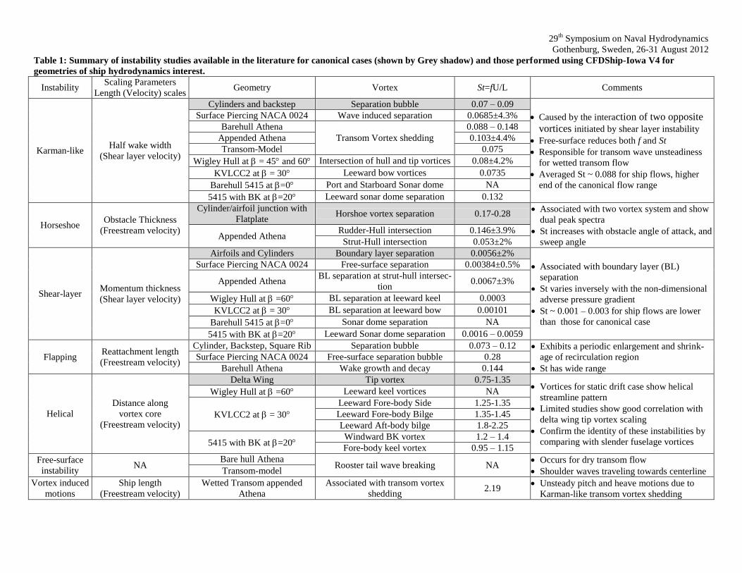
29th
Symposium on Naval Hydrodynamics
Gothenburg, Sweden, 26-31 August 2012
Table 1: Summary of instability studies available in the literature for canonical cases (shown by Grey shadow) and those performed using CFDShip-Iowa V4 for
geometries of ship hydrodynamics interest.
Instability Scaling Parameters
Length (Velocity) scales Geometry Vortex St=fU/L Comments
Karman-like Half wake width
(Shear layer velocity)
Cylinders and backstep Separation bubble 0.07 – 0.09
Caused by the interaction of two opposite
vortices initiated by shear layer instability
Free-surface reduces both f and St
Responsible for transom wave unsteadiness
for wetted transom flow
Averaged St ~ 0.088 for ship flows, higher
end of the canonical flow range
Surface Piercing NACA 0024 Wave induced separation 0.0685±4.3%
Barehull Athena
Transom Vortex shedding
0.088 – 0.148
Appended Athena 0.103±4.4%
Transom-Model 0.075
Wigley Hull at = 45 and 60 Intersection of hull and tip vortices 0.08±4.2%
KVLCC2 at = 30 Leeward bow vortices 0.0735
Barehull 5415 at =0 Port and Starboard Sonar dome NA
5415 with BK at =20 Leeward sonar dome separation 0.132
Horseshoe Obstacle Thickness
(Freestream velocity)
Cylinder/airfoil junction with
Flatplate Horshoe vortex separation 0.17-0.28
Associated with two vortex system and show
dual peak spectra
St increases with obstacle angle of attack, and
sweep angle Appended Athena
Rudder-Hull intersection 0.146±3.9%
Strut-Hull intersection 0.053±2%
Shear-layer Momentum thickness
(Shear layer velocity)
Airfoils and Cylinders Boundary layer separation 0.0056±2%
Associated with boundary layer (BL)
separation
St varies inversely with the non-dimensional
adverse pressure gradient
St ~ 0.001 – 0.003 for ship flows are lower
than those for canonical case
Surface Piercing NACA 0024 Free-surface separation 0.00384±0.5%
Appended Athena BL separation at strut-hull intersec-
tion 0.0067±3%
Wigley Hull at =60 BL separation at leeward keel 0.0003
KVLCC2 at = 30 BL separation at leeward bow 0.00101
Barehull 5415 at =0 Sonar dome separation NA
5415 with BK at =20 Leeward Sonar dome separation 0.0016 – 0.0059
Flapping Reattachment length
(Freestream velocity)
Cylinder, Backstep, Square Rib Separation bubble 0.073 – 0.12 Exhibits a periodic enlargement and shrink-
age of recirculation region
St has wide range
Surface Piercing NACA 0024 Free-surface separation bubble 0.28
Barehull Athena Wake growth and decay 0.144
Helical
Distance along
vortex core
(Freestream velocity)
Delta Wing Tip vortex 0.75-1.35 Vortices for static drift case show helical
streamline pattern
Limited studies show good correlation with
delta wing tip vortex scaling
Confirm the identity of these instabilities by
comparing with slender fuselage vortices
Wigley Hull at =60 Leeward keel vortices NA
KVLCC2 at = 30
Leeward Fore-body Side 1.25-1.35
Leeward Fore-body Bilge 1.35-1.45
Leeward Aft-body bilge 1.8-2.25
5415 with BK at =20 Windward BK vortex 1.2 – 1.4
Fore-body keel vortex 0.95 – 1.15
Free-surface
instability NA
Bare hull Athena Rooster tail wave breaking NA
Occurs for dry transom flow
Shoulder waves traveling towards centerline Transom-model
Vortex induced
motions
Ship length
(Freestream velocity)
Wetted Transom appended
Athena
Associated with transom vortex
shedding 2.19
Unsteady pitch and heave motions due to
Karman-like transom vortex shedding
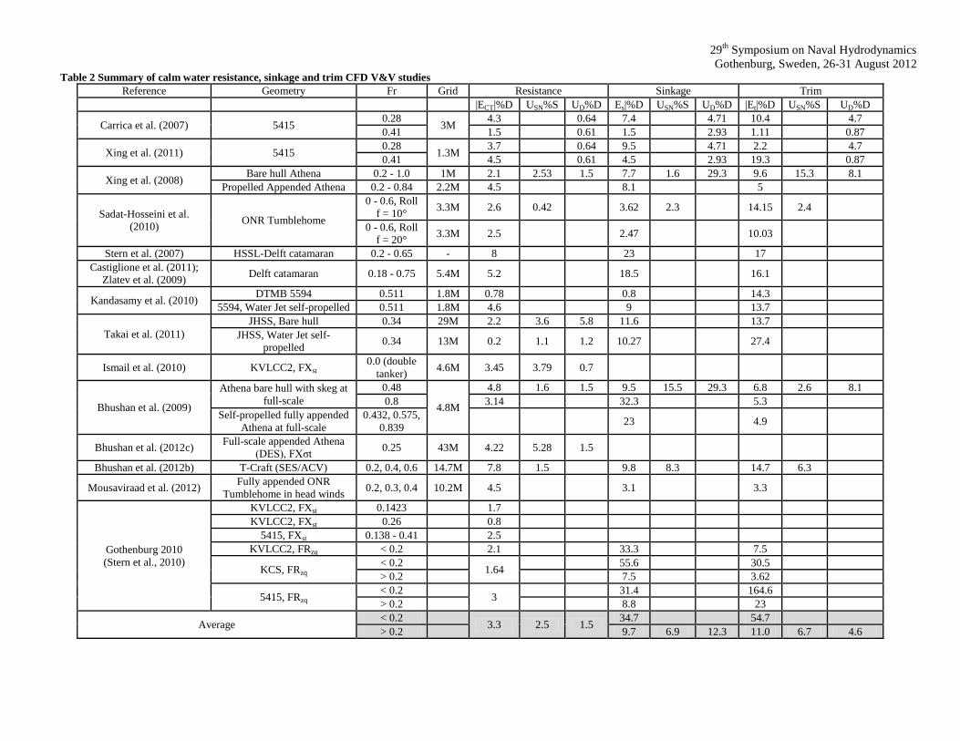
29th
Symposium on Naval Hydrodynamics
Gothenburg, Sweden, 26-31 August 2012 Table 2 Summary of calm water resistance, sinkage and trim CFD V&V studies
Reference Geometry Fr Grid Resistance Sinkage Trim
|ECT|%D USN%S UD%D Es|%D USN%S UD%D |Et|%D USN%S UD%D
Carrica et al. (2007) 5415 0.28
3M 4.3
0.64 7.4
4.71 10.4
4.7
0.41 1.5
0.61 1.5
2.93 1.11
0.87
Xing et al. (2011) 5415 0.28
1.3M 3.7
0.64 9.5
4.71 2.2
4.7
0.41 4.5
0.61 4.5
2.93 19.3
0.87
Xing et al. (2008) Bare hull Athena 0.2 - 1.0 1M 2.1 2.53 1.5 7.7 1.6 29.3 9.6 15.3 8.1
Propelled Appended Athena 0.2 - 0.84 2.2M 4.5
8.1
5
Sadat-Hosseini et al.
(2010) ONR Tumblehome
0 - 0.6, Roll
f = 10° 3.3M 2.6 0.42
3.62 2.3
14.15 2.4
0 - 0.6, Roll
f = 20° 3.3M 2.5
2.47
10.03
Stern et al. (2007) HSSL-Delft catamaran 0.2 - 0.65 - 8
23
17
Castiglione et al. (2011);
Zlatev et al. (2009) Delft catamaran 0.18 - 0.75 5.4M 5.2
18.5
16.1
Kandasamy et al. (2010) DTMB 5594 0.511 1.8M 0.78
0.8
14.3
5594, Water Jet self-propelled 0.511 1.8M 4.6
9
13.7
Takai et al. (2011)
JHSS, Bare hull 0.34 29M 2.2 3.6 5.8 11.6
13.7
JHSS, Water Jet self-
propelled 0.34 13M 0.2 1.1 1.2 10.27
27.4
Ismail et al. (2010) KVLCC2, FXst 0.0 (double
tanker) 4.6M 3.45 3.79 0.7
Bhushan et al. (2009)
Athena bare hull with skeg at
full-scale
0.48
4.8M
4.8 1.6 1.5 9.5 15.5 29.3 6.8 2.6 8.1
0.8 3.14
32.3
5.3
Self-propelled fully appended
Athena at full-scale
0.432, 0.575,
0.839 23
4.9
Bhushan et al. (2012c) Full-scale appended Athena
(DES), FXσt 0.25 43M 4.22 5.28 1.5
Bhushan et al. (2012b) T-Craft (SES/ACV) 0.2, 0.4, 0.6 14.7M 7.8 1.5
9.8 8.3
14.7 6.3
Mousaviraad et al. (2012) Fully appended ONR
Tumblehome in head winds 0.2, 0.3, 0.4 10.2M 4.5
3.1
3.3
Gothenburg 2010
(Stern et al., 2010)
KVLCC2, FXst 0.1423
1.7
KVLCC2, FXst 0.26
0.8
5415, FXst 0.138 - 0.41
2.5
KVLCC2, FRzq < 0.2
2.1
33.3
7.5
KCS, FRzq < 0.2
1.64 55.6
30.5
> 0.2
7.5
3.62
5415, FRzq < 0.2
3 31.4
164.6
> 0.2
8.8
23
Average < 0.2
3.3 2.5 1.5 34.7
54.7
> 0.2
9.7 6.9 12.3 11.0 6.7 4.6
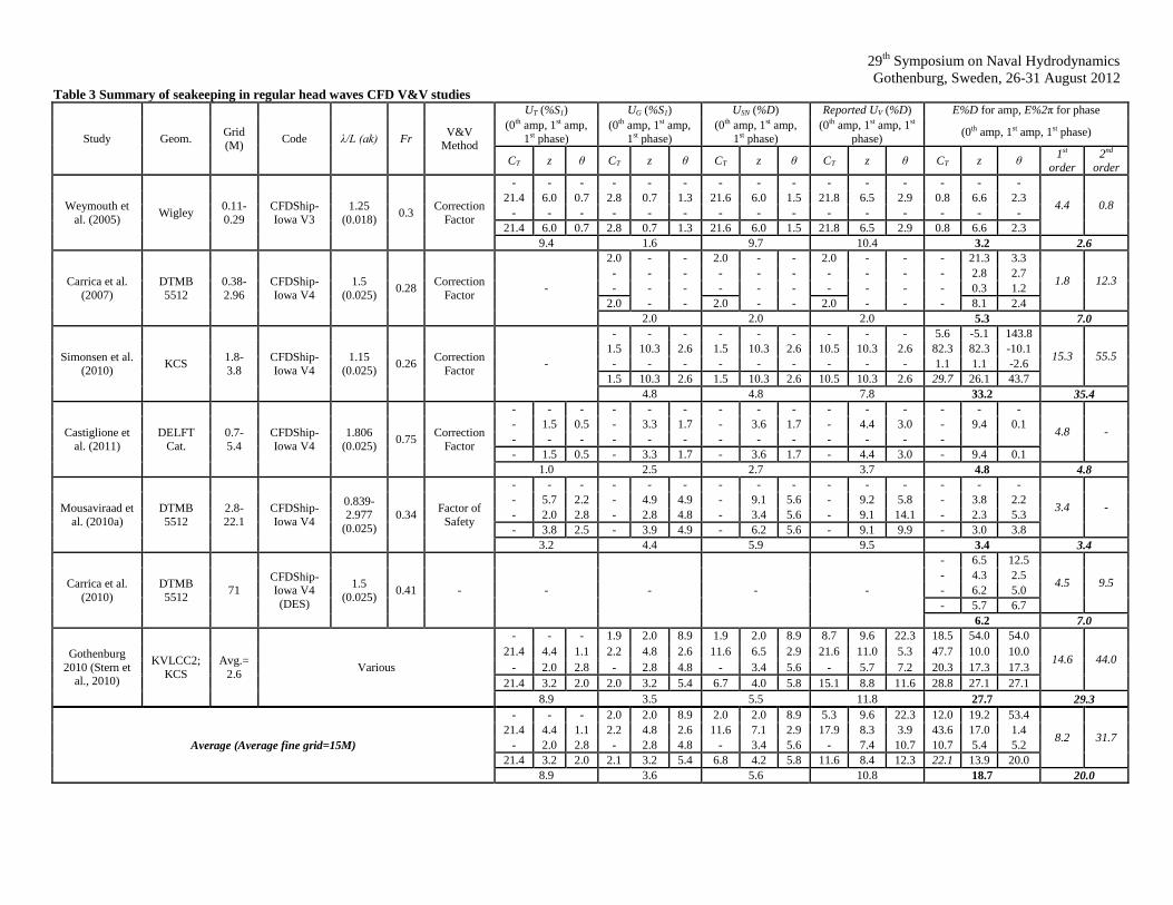
29th
Symposium on Naval Hydrodynamics
Gothenburg, Sweden, 26-31 August 2012 Table 3 Summary of seakeeping in regular head waves CFD V&V studies
Study Geom. Grid (M)
Code λ/L (ak) Fr V&V
Method
UT (%S1) UG (%S1) USN (%D) Reported UV (%D) E%D for amp, E%2π for phase
(0th amp, 1st amp,
1st phase)
(0th amp, 1st amp,
1st phase)
(0th amp, 1st amp,
1st phase)
(0th amp, 1st amp, 1st
phase) (0th amp, 1st amp, 1st phase)
CT z θ CT z θ CT z θ CT z θ CT z θ 1st
order
2nd
order
Weymouth et
al. (2005) Wigley
0.11-
0.29
CFDShip-
Iowa V3
1.25
(0.018) 0.3
Correction
Factor
- - - - - - - - - - - - - - -
4.4 0.8 21.4 6.0 0.7 2.8 0.7 1.3 21.6 6.0 1.5 21.8 6.5 2.9 0.8 6.6 2.3
- - - - - - - - - - - - - - -
21.4 6.0 0.7 2.8 0.7 1.3 21.6 6.0 1.5 21.8 6.5 2.9 0.8 6.6 2.3
9.4 1.6 9.7 10.4 3.2 2.6
Carrica et al.
(2007)
DTMB
5512
0.38-
2.96
CFDShip-
Iowa V4
1.5
(0.025) 0.28
Correction
Factor -
2.0 - - 2.0 - - 2.0 - - - 21.3 3.3
1.8 12.3 - - - - - - - - - - 2.8 2.7
- - - - - - - - - - 0.3 1.2
2.0 - - 2.0 - - 2.0 - - - 8.1 2.4
2.0 2.0 2.0 5.3 7.0
Simonsen et al.
(2010) KCS
1.8-
3.8
CFDShip-
Iowa V4
1.15
(0.025) 0.26
Correction
Factor -
- - - - - - - - - 5.6 -5.1 143.8
15.3 55.5 1.5 10.3 2.6 1.5 10.3 2.6 10.5 10.3 2.6 82.3 82.3 -10.1
- - - - - - - - - 1.1 1.1 -2.6
1.5 10.3 2.6 1.5 10.3 2.6 10.5 10.3 2.6 29.7 26.1 43.7
4.8 4.8 7.8 33.2 35.4
Castiglione et
al. (2011)
DELFT
Cat.
0.7-
5.4
CFDShip-
Iowa V4
1.806
(0.025) 0.75
Correction
Factor
- - - - - - - - - - - - - - -
4.8 - - 1.5 0.5 - 3.3 1.7 - 3.6 1.7 - 4.4 3.0 - 9.4 0.1
- - - - - - - - - - - - -
- 1.5 0.5 - 3.3 1.7 - 3.6 1.7 - 4.4 3.0 - 9.4 0.1
1.0 2.5 2.7 3.7 4.8 4.8
Mousaviraad et
al. (2010a)
DTMB
5512
2.8-
22.1
CFDShip-
Iowa V4
0.839-2.977
(0.025)
0.34 Factor of
Safety
- - - - - - - - - - - - - - -
3.4 - - 5.7 2.2 - 4.9 4.9 - 9.1 5.6 - 9.2 5.8 - 3.8 2.2
- 2.0 2.8 - 2.8 4.8 - 3.4 5.6 - 9.1 14.1 - 2.3 5.3
- 3.8 2.5 - 3.9 4.9 - 6.2 5.6 - 9.1 9.9 - 3.0 3.8
3.2 4.4 5.9 9.5 3.4 3.4
Carrica et al.
(2010)
DTMB
5512 71
CFDShip-Iowa V4
(DES)
1.5
(0.025) 0.41 - - - - -
- 6.5 12.5
4.5 9.5 - 4.3 2.5
- 6.2 5.0
- 5.7 6.7
6.2 7.0
Gothenburg
2010 (Stern et al., 2010)
KVLCC2;
KCS
Avg.=
2.6 Various
- - - 1.9 2.0 8.9 1.9 2.0 8.9 8.7 9.6 22.3 18.5 54.0 54.0
14.6 44.0 21.4 4.4 1.1 2.2 4.8 2.6 11.6 6.5 2.9 21.6 11.0 5.3 47.7 10.0 10.0
- 2.0 2.8 - 2.8 4.8 - 3.4 5.6 - 5.7 7.2 20.3 17.3 17.3
21.4 3.2 2.0 2.0 3.2 5.4 6.7 4.0 5.8 15.1 8.8 11.6 28.8 27.1 27.1
8.9 3.5 5.5 11.8 27.7 29.3
Average (Average fine grid=15M)
- - - 2.0 2.0 8.9 2.0 2.0 8.9 5.3 9.6 22.3 12.0 19.2 53.4
8.2 31.7 21.4 4.4 1.1 2.2 4.8 2.6 11.6 7.1 2.9 17.9 8.3 3.9 43.6 17.0 1.4
- 2.0 2.8 - 2.8 4.8 - 3.4 5.6 - 7.4 10.7 10.7 5.4 5.2
21.4 3.2 2.0 2.1 3.2 5.4 6.8 4.2 5.8 11.6 8.4 12.3 22.1 13.9 20.0
8.9 3.6 5.6 10.8 18.7 20.0
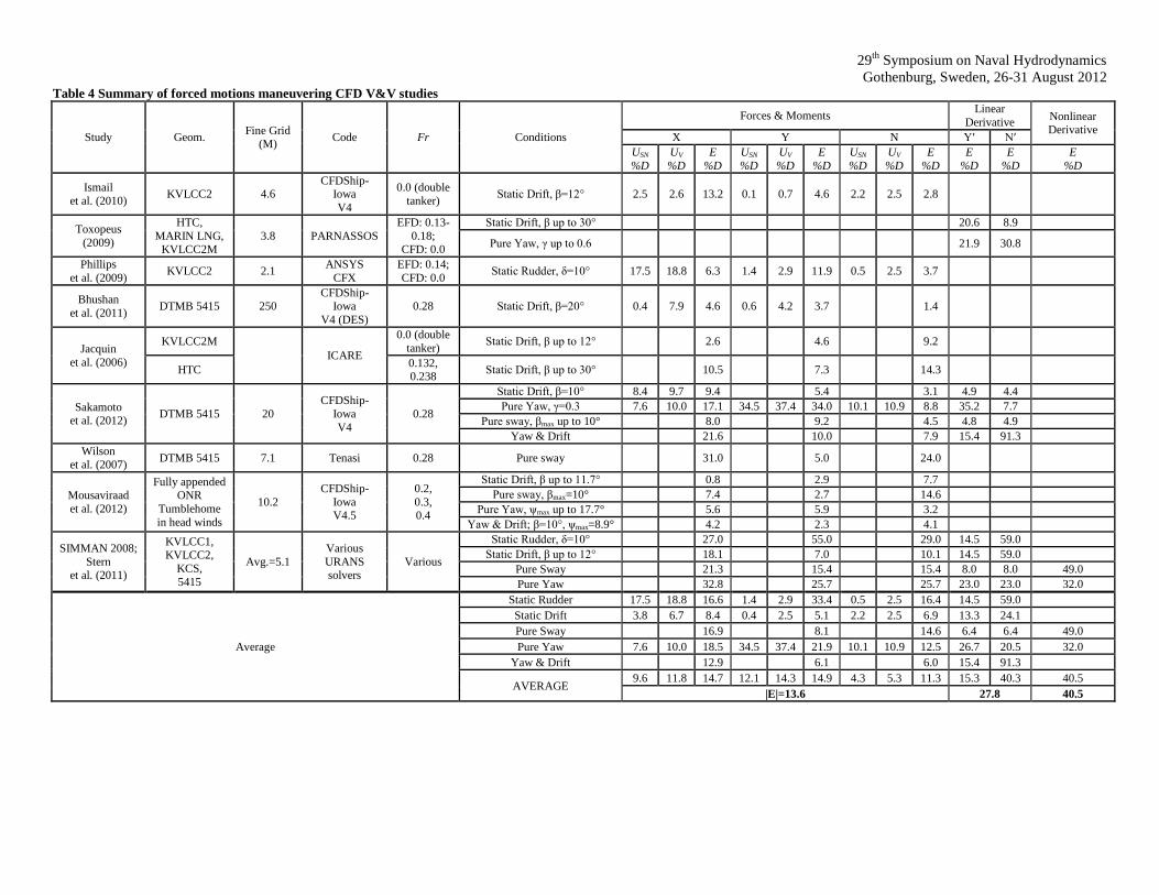
29th
Symposium on Naval Hydrodynamics
Gothenburg, Sweden, 26-31 August 2012 Table 4 Summary of forced motions maneuvering CFD V&V studies
Study Geom. Fine Grid
(M) Code Fr Conditions
Forces & Moments Linear
Derivative Nonlinear Derivative
X Y N Yʹ Nʹ
USN
%D
UV
%D
E
%D
USN
%D
UV
%D
E
%D
USN
%D
UV
%D
E
%D
E
%D
E
%D
E
%D
Ismail
et al. (2010) KVLCC2 4.6
CFDShip-Iowa
V4
0.0 (double
tanker) Static Drift, β=12° 2.5 2.6 13.2 0.1 0.7 4.6 2.2 2.5 2.8
Toxopeus
(2009)
HTC,
MARIN LNG, KVLCC2M
3.8 PARNASSOS
EFD: 0.13-
0.18; CFD: 0.0
Static Drift, β up to 30°
20.6 8.9
Pure Yaw, γ up to 0.6
21.9 30.8
Phillips
et al. (2009) KVLCC2 2.1
ANSYS
CFX
EFD: 0.14;
CFD: 0.0 Static Rudder, δ=10° 17.5 18.8 6.3 1.4 2.9 11.9 0.5 2.5 3.7
Bhushan
et al. (2011) DTMB 5415 250
CFDShip-Iowa
V4 (DES)
0.28 Static Drift, β=20° 0.4 7.9 4.6 0.6 4.2 3.7
1.4
Jacquin
et al. (2006)
KVLCC2M
ICARE
0.0 (double
tanker) Static Drift, β up to 12°
2.6
4.6
9.2
HTC
0.132, 0.238
Static Drift, β up to 30°
10.5
7.3
14.3
Sakamoto
et al. (2012) DTMB 5415 20
CFDShip-
Iowa
V4
0.28
Static Drift, β=10° 8.4 9.7 9.4
5.4
3.1 4.9 4.4 Pure Yaw, γ=0.3 7.6 10.0 17.1 34.5 37.4 34.0 10.1 10.9 8.8 35.2 7.7 Pure sway, βmax up to 10°
8.0
9.2
4.5 4.8 4.9
Yaw & Drift
21.6
10.0
7.9 15.4 91.3 Wilson
et al. (2007) DTMB 5415 7.1 Tenasi 0.28 Pure sway
31.0
5.0
24.0
Mousaviraad
et al. (2012)
Fully appended ONR
Tumblehome
in head winds
10.2
CFDShip-
Iowa V4.5
0.2,
0.3, 0.4
Static Drift, β up to 11.7°
0.8
2.9
7.7 Pure sway, βmax=10°
7.4
2.7
14.6
Pure Yaw, ψmax up to 17.7°
5.6
5.9
3.2 Yaw & Drift; β=10°, ψmax=8.9°
4.2
2.3
4.1
SIMMAN 2008;
Stern et al. (2011)
KVLCC1, KVLCC2,
KCS,
5415
Avg.=5.1
Various
URANS solvers
Various
Static Rudder, δ=10°
27.0
55.0
29.0 14.5 59.0 Static Drift, β up to 12°
18.1
7.0
10.1 14.5 59.0
Pure Sway
21.3
15.4
15.4 8.0 8.0 49.0
Pure Yaw
32.8
25.7
25.7 23.0 23.0 32.0
Average
Static Rudder 17.5 18.8 16.6 1.4 2.9 33.4 0.5 2.5 16.4 14.5 59.0 Static Drift 3.8 6.7 8.4 0.4 2.5 5.1 2.2 2.5 6.9 13.3 24.1 Pure Sway
16.9
8.1
14.6 6.4 6.4 49.0
Pure Yaw 7.6 10.0 18.5 34.5 37.4 21.9 10.1 10.9 12.5 26.7 20.5 32.0
Yaw & Drift
12.9
6.1
6.0 15.4 91.3
AVERAGE 9.6 11.8 14.7 12.1 14.3 14.9 4.3 5.3 11.3 15.3 40.3 40.5
|E|=13.6 27.8 40.5
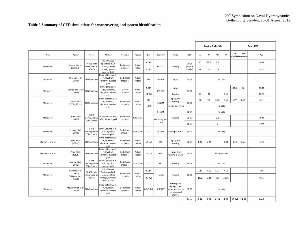
29th
Symposium on Naval Hydrodynamics
Gothenburg, Sweden, 26-31 August 2012
Table 5 Summary of CFD simulations for maneuvering and system identification
Turning Circle E%D Zigzag E%D
Type Author Code Method Propulsion Rudder Grid Geometry Cases DOF A TR TD D 1st
overshoot 2nd
overshoot Ave.
Maneuver Muscari et al.
(2008a,b)
RANSE code developed at
INSAEN
Finite Volume, Spalart and All- Maras, no free
surface,dynamic overset Grid
Body force propeller
Actual rudder
424K
KVLCC2 turning 3DOF
(double model)
6.2 11.2 7.2
8.20
3.4M 8.4 5.3 0.8
4.83
Maneuver Bhushan et al.
(2009) CFDShip-Iowa
Finite difference, k-w, level set,
dynamic overset grid
Body force propeller
Actual rudder
7M 5415M zigzag 6DOF No data
Maneuver Carrica and Stern
(2008) CFDShip-Iowa
Finite difference, DES, level set,
dynamic overset grid
Actual propeller
Actual rudder
5.6M
KVLCC1
zigzag
6DOF
30.6 36 33.30
14.9M turning 8 24
0.65
10.88
Maneuver Carrica et al.
(2008a,2012a) CFDShip-Iowa
Finite difference, k-w, level set,
dynamic overset grid
Body force propeller
Actual rudder
7M
5415M
zigzag and turning
6DOF
2.6 9.5 5.18 5.69 6.97 6.69 6.11
12M turning in waves No data
Maneuver Drouet et al.
(2008)
ICARE developed by ECN, France
Finite volume, k-w, VOF, dynamic grid
Body force propeller
Side force -
5415M
turning
6DOF No data
Humburg test case
3DOF
0.3
0.30
6DOF
5
5.00
Maneuver Ferrant et al.
(2008)
ICARE developed by ECN, France
Finite volume, k-w, VOF, dynamic overset grid
Body force propeller
Side force - 5415M Turning in waves 6DOF No data
Maneuver and SI Araki et al.
(2012a) CFDShip-Iowa
Finite difference, k-w, level set,
dynamic overset grid
Body force propeller
Actual rudder
12.1M OT zigzag and
turning 6DOF 1.23 2.29
1.34 1.54 2.23 1.73
Maneuver and SI Araki et al.
(2012b) CFDShip-Iowa
Finite difference, k-w, level set,
dynamic overset grid
Body force propeller
Actual rudder
12.1M OT zigzag and
turning in wave 6DOF Not reported
Maneuver Jacquin et al.
(2006)
ICARE developed by ECN, France
Finite volume, k-w, VOF, dynamic overset grid
Body force propeller
Side force - S60 turning 6DOF No data
Maneuver
Durante et al. (2010)
Dubbioso et al. (2012)
RANSE code developed at
INSAEN
Finite Volume, Spalart and All-Maras, no free
surface, dynamic overset Grid
Body force propeller
Actual rudder
6.2M
Tanker turning 6DOF
7.35 3.15 5.24 4.06
4.95
0.77M 10.6 9.42 4.96 12.26
9.31
Maneuver Mousaviraad et al.
(2012) CFDShip-Iowa
Finite difference, k-w, level set,
dynamic overset grid
Body force propeller
Actual rudder
8.6-9.3M SES/ACV
turning and zigzag in calm
water and waves for deep and
shallow
6DOF No data
Total 6.34 9.27 4.10 4.80 13.04 14.97 8.46
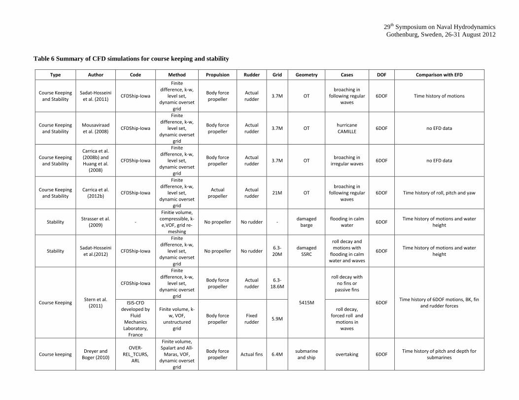
29th
Symposium on Naval Hydrodynamics
Gothenburg, Sweden, 26-31 August 2012
Table 6 Summary of CFD simulations for course keeping and stability
Type Author Code Method Propulsion Rudder Grid Geometry Cases DOF Comparison with EFD
Course Keeping and Stability
Sadat-Hosseini et al. (2011)
CFDShip-Iowa
Finite difference, k-w,
level set, dynamic overset
grid
Body force propeller
Actual rudder
3.7M OT broaching in
following regular waves
6DOF Time history of motions
Course Keeping and Stability
Mousaviraad et al. (2008)
CFDShip-Iowa
Finite difference, k-w,
level set, dynamic overset
grid
Body force propeller
Actual rudder
3.7M OT hurricane CAMILLE
6DOF no EFD data
Course Keeping and Stability
Carrica et al. (2008b) and Huang et al.
(2008)
CFDShip-Iowa
Finite difference, k-w,
level set, dynamic overset
grid
Body force propeller
Actual rudder
3.7M OT broaching in
irregular waves 6DOF no EFD data
Course Keeping and Stability
Carrica et al. (2012b)
CFDShip-Iowa
Finite difference, k-w,
level set, dynamic overset
grid
Actual propeller
Actual rudder
21M OT broaching in
following regular waves
6DOF Time history of roll, pitch and yaw
Stability Strasser et al.
(2009) -
Finitie volume, compressible, k-e,VOF, grid re-
meshing
No propeller No rudder - damaged
barge flooding in calm
water 6DOF
Time history of motions and water height
Stability Sadat-Hosseini
et al.(2012) CFDShip-Iowa
Finite difference, k-w,
level set, dynamic overset
grid
No propeller No rudder 6.3-20M
damaged SSRC
roll decay and motions with
flooding in calm water and waves
6DOF Time history of motions and water
height
Course Keeping Stern et al.
(2011)
CFDShip-Iowa
Finite difference, k-w,
level set, dynamic overset
grid
Body force propeller
Actual rudder
6.3-18.6M
5415M
roll decay with no fins or
passive fins
6DOF Time history of 6DOF motions, BK, fin
and rudder forces ISIS-CFD
developed by Fluid
Mechanics Laboratory,
France
Finite volume, k-w, VOF,
unstructured grid
Body force propeller
Fixed rudder
5.9M
roll decay, forced roll and
motions in waves
Course keeping Dreyer and
Boger (2010)
OVER-REL_TCURS,
ARL
Finite volume, Spalart and All-
Maras, VOF, dynamic overset
grid
Body force propeller
Actual fins 6.4M submarine and ship
overtaking 6DOF Time history of pitch and depth for
submarines
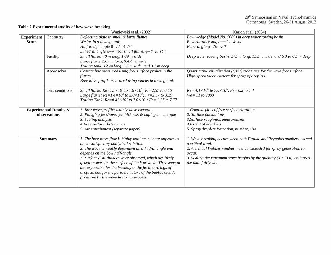
29th
Symposium on Naval Hydrodynamics
Gothenburg, Sweden, 26-31 August 2012
Table 7 Experimental studies of bow wave breaking
Waniewski et al. (2002) Karion et al. (2004)
Experiment
Setup
Geometry Deflecting plate in small & large flumes
Wedge in a towing tank
Half wedge angle θ=13˚ & 26˚
Dihedral angle φ=0˚ (for small flume, φ=0˚ to 15˚)
Bow wedge (Model No. 5605) in deep water towing basin
Bow entrance angle θ=20˚ & 40˚
Flare angle φ=20˚ & 0˚
Facility Small flume: 40 m long, 1.09 m wide
Large flume:2.65 m long, 0.459 m wide
Towing tank: 126m long, 7.5 m wide, and 3.7 m deep
Deep water towing basin: 575 m long, 15.5 m wide, and 6.3 to 6.5 m deep.
Approaches Contact line measured using free surface probes in the
flumes
Bow wave profile measured using videos in towing tank
Quantitative visualization (QViz) technique for the wave free surface
High-speed video camera for spray of droplets
Test conditions Small flume: Re=1.1×10⁴ to 1.6×10
4; Fr=2.57 to 6.46
Large flume: Re=1.4×10⁵ to 2.0×10
5; Fr=2.57 to 3.29
Towing Tank: Re=0.43×10⁵ to 7.0×10
5; Fr= 1.27 to 7.77
Re= 4.1×10⁵ to 7.0×10
6; Fr= 0.2 to 1.4
We= 11 to 2800
Experimental Results &
observations
1. Bow wave profile: mainly wave elevation
2. Plunging jet shape: jet thickness & impingement angle
3. Scaling analysis
4.Free surface disturbance
5. Air entrainment (separate paper)
1.Contour plots of free surface elevation
2. Surface fluctuations
3.Surface roughness measurement
4.Extent of breaking
5. Spray droplets formation, number, size
Summary 1. The bow wave flow is highly nonlinear, there appears to
be no satisfactory analytical solution.
2. The wave is weakly dependent on dihedral angle and
depends on the bow half-angle.
3. Surface disturbances were observed, which are likely
gravity waves on the surface of the bow wave. They seem to
be responsible for the breakup of the jet into strings of
droplets and for the periodic nature of the bubble clouds
produced by the wave breaking process.
1. Wave breaking occurs when both Froude and Reynolds numbers exceed
a critical level.
2. A critical Webber number must be exceeded for spray generation to
occur.
3. Scaling the maximum wave heights by the quantity ( Fr1.5
D), collapses
the data fairly well.
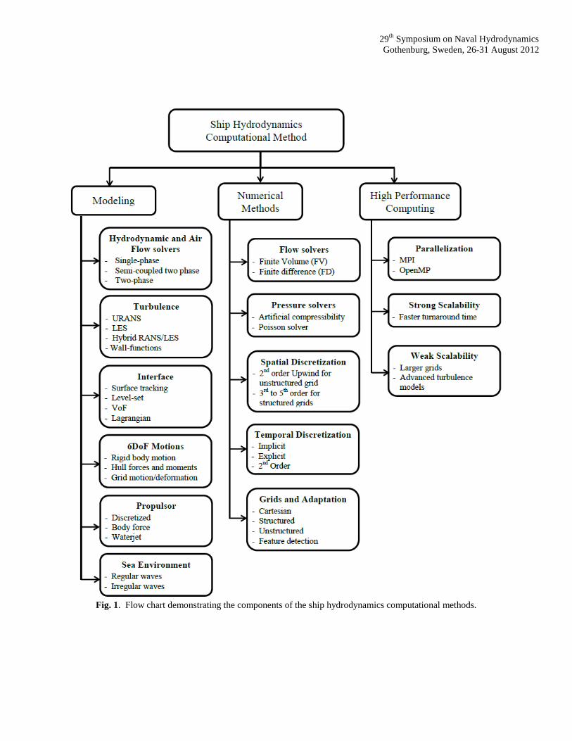
29th
Symposium on Naval Hydrodynamics
Gothenburg, Sweden, 26-31 August 2012
Fig. 1. Flow chart demonstrating the components of the ship hydrodynamics computational methods.
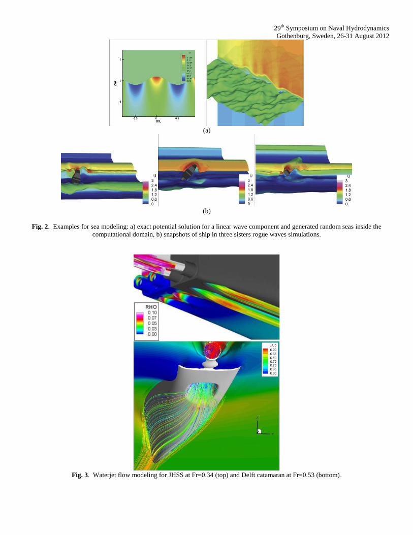
29th
Symposium on Naval Hydrodynamics
Gothenburg, Sweden, 26-31 August 2012
(a)
(b)
Fig. 2. Examples for sea modeling: a) exact potential solution for a linear wave component and generated random seas inside the
computational domain, b) snapshots of ship in three sisters rogue waves simulations.
Fig. 3. Waterjet flow modeling for JHSS at Fr=0.34 (top) and Delft catamaran at Fr=0.53 (bottom).
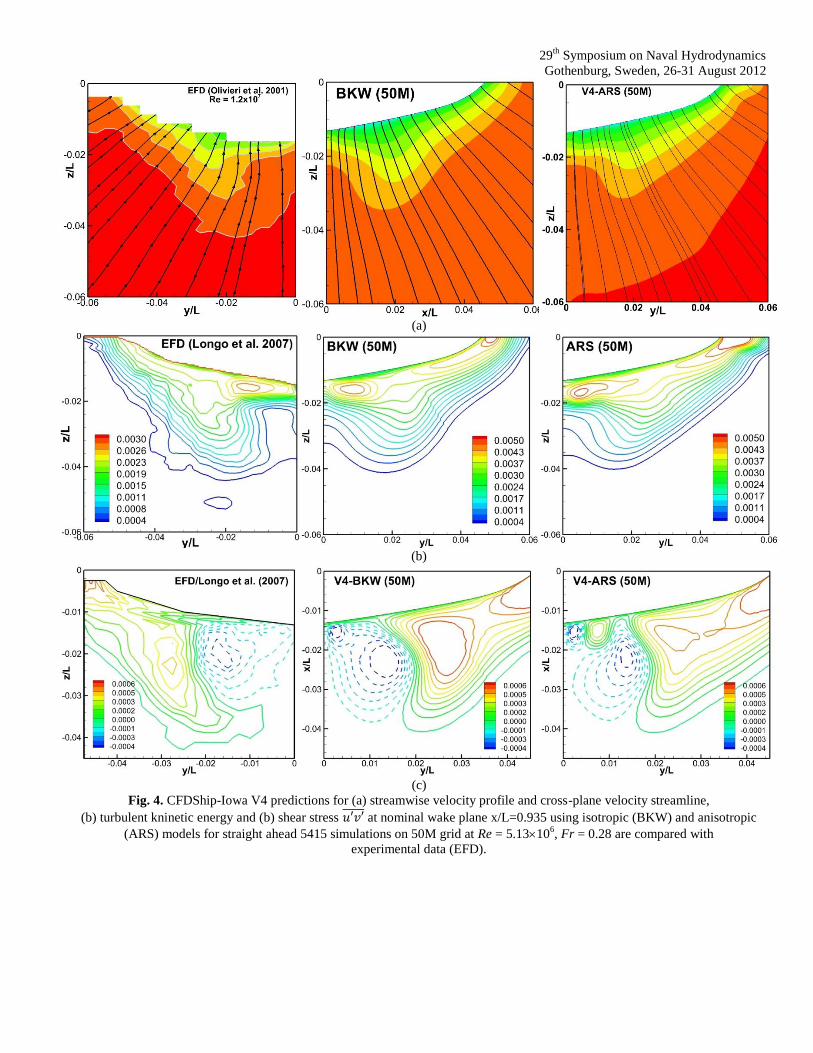
29th
Symposium on Naval Hydrodynamics
Gothenburg, Sweden, 26-31 August 2012
(a)
(b)
(c)
Fig. 4. CFDShip-Iowa V4 predictions for (a) streamwise velocity profile and cross-plane velocity streamline,
(b) turbulent kninetic energy and (b) shear stress at nominal wake plane x/L=0.935 using isotropic (BKW) and anisotropic
(ARS) models for straight ahead 5415 simulations on 50M grid at Re = 5.13106, Fr = 0.28 are compared with
experimental data (EFD).
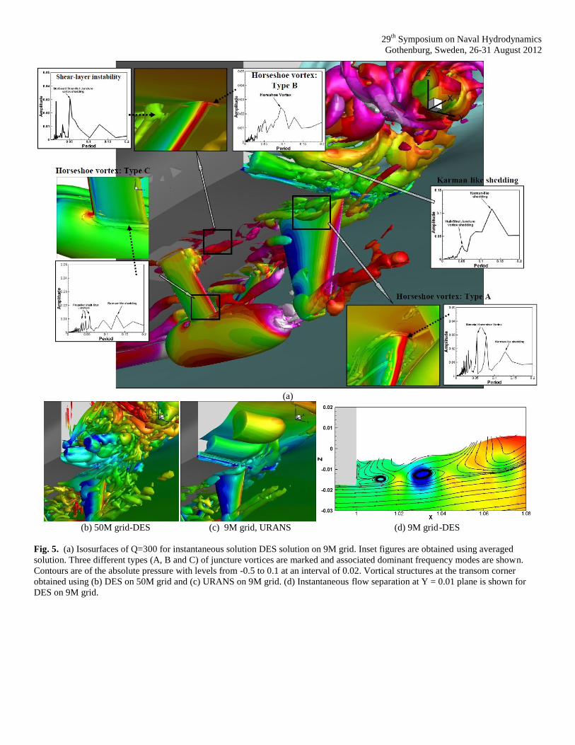
29th
Symposium on Naval Hydrodynamics
Gothenburg, Sweden, 26-31 August 2012
(a)
(b) 50M grid-DES (c) 9M grid, URANS (d) 9M grid-DES
Fig. 5. (a) Isosurfaces of Q=300 for instantaneous solution DES solution on 9M grid. Inset figures are obtained using averaged
solution. Three different types (A, B and C) of juncture vortices are marked and associated dominant frequency modes are shown.
Contours are of the absolute pressure with levels from -0.5 to 0.1 at an interval of 0.02. Vortical structures at the transom corner
obtained using (b) DES on 50M grid and (c) URANS on 9M grid. (d) Instantaneous flow separation at Y = 0.01 plane is shown for
DES on 9M grid.
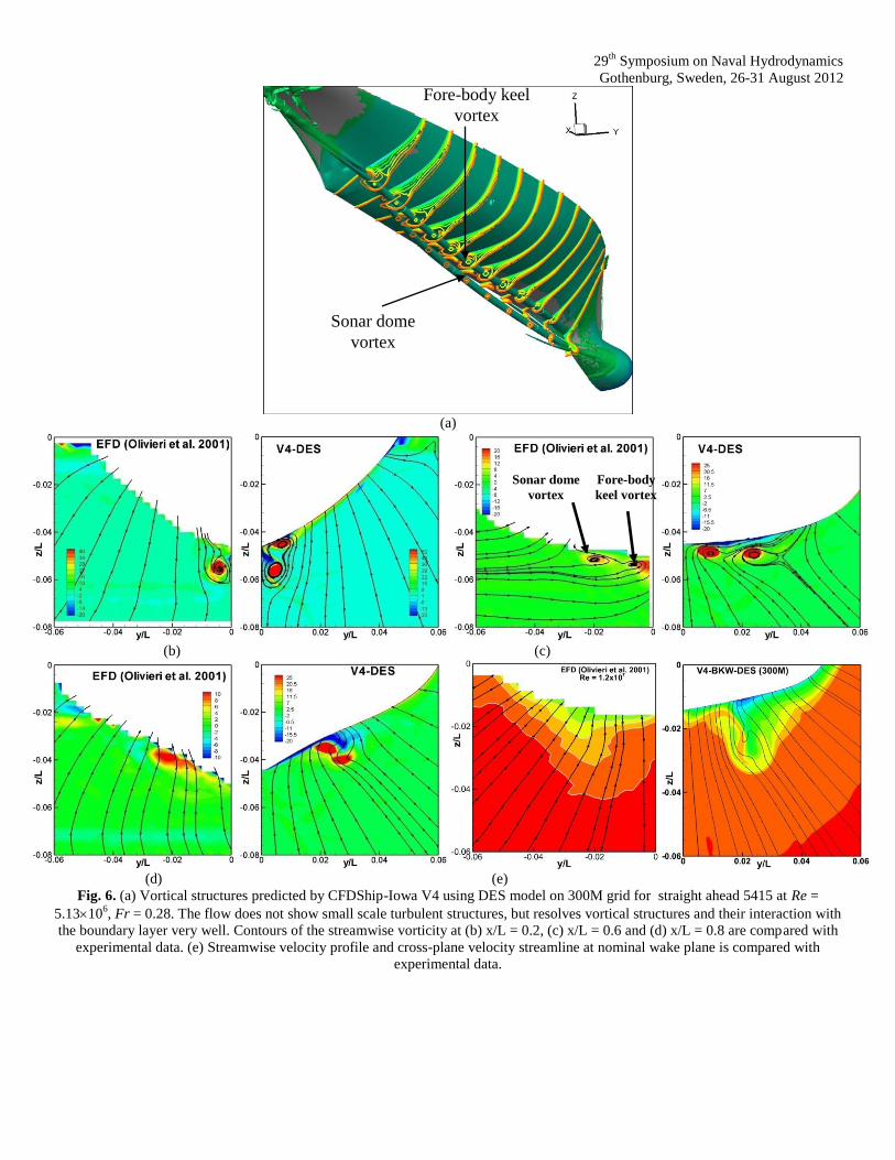
29th
Symposium on Naval Hydrodynamics
Gothenburg, Sweden, 26-31 August 2012
(a)
(b) (c)
(d) (e)
Fig. 6. (a) Vortical structures predicted by CFDShip-Iowa V4 using DES model on 300M grid for straight ahead 5415 at Re =
5.13106, Fr = 0.28. The flow does not show small scale turbulent structures, but resolves vortical structures and their interaction with
the boundary layer very well. Contours of the streamwise vorticity at (b) x/L = 0.2, (c) x/L = 0.6 and (d) x/L = 0.8 are compared with
experimental data. (e) Streamwise velocity profile and cross-plane velocity streamline at nominal wake plane is compared with
experimental data.
Sonar dome
vortex
Fore-body
keel vortex
Fore-body keel
vortex
Sonar dome
vortex
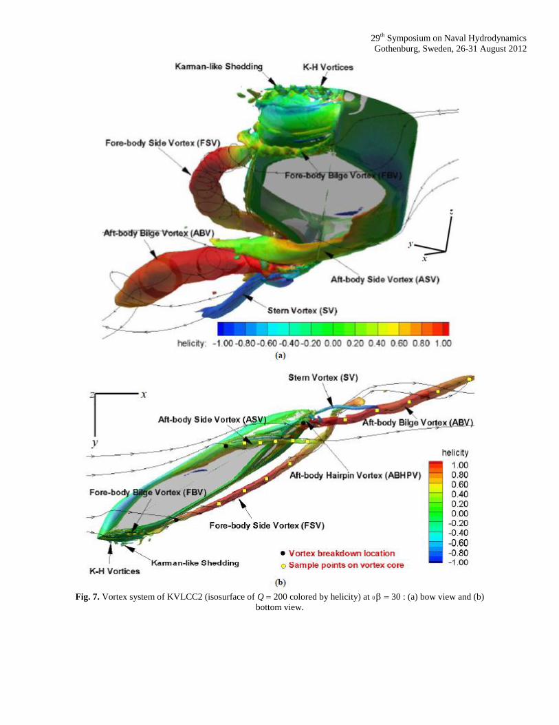
29th
Symposium on Naval Hydrodynamics
Gothenburg, Sweden, 26-31 August 2012
Fig. 7. Vortex system of KVLCC2 (isosurface of Q 200 colored by helicity) at 0 30 : (a) bow view and (b)
bottom view.
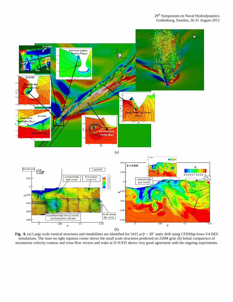
29th
Symposium on Naval Hydrodynamics
Gothenburg, Sweden, 26-31 August 2012
(a)
(b)
Fig. 8. (a) Large scale vortical structures and instabilities are identified for 5415 at = 20 static drift using CFDShip-Iowa V4 DES
simulations. The inset on right topmost corner shows the small scale structures predicted on 250M grid. (b) Initial comparison of
streamwise velocity contour and cross flow vectors and wake at X=0.935 shows very good agreement with the ongoing experiments.
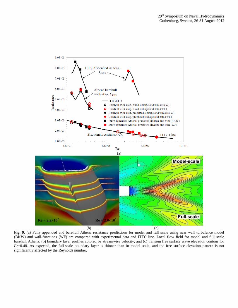
29th
Symposium on Naval Hydrodynamics
Gothenburg, Sweden, 26-31 August 2012
(a)
(b) (c)
Fig. 9. (a) Fully appended and barehull Athena resistance predictions for model and full scale using near wall turbulence model
(BKW) and wall-functions (WF) are compared with experimental data and ITTC line. Local flow field for model and full scale
barehull Athena: (b) boundary layer profiles colored by streamwise velocity; and (c) transom free surface wave elevation contour for
Fr=0.48. As expected, the full-scale boundary layer is thinner than in model-scale, and the free surface elevation pattern is not
significantly affected by the Reynolds number.
Re = 2.2107
Re = 2.0109
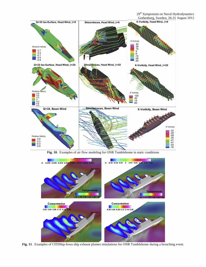
29th
Symposium on Naval Hydrodynamics
Gothenburg, Sweden, 26-31 August 2012
Fig. 10. Examples of air flow modeling for ONR Tumblehome in static conditions
Fig. 11. Examples of CFDShip-Iowa ship exhaust plumes simulations for ONR Tumblehome during a broaching event.
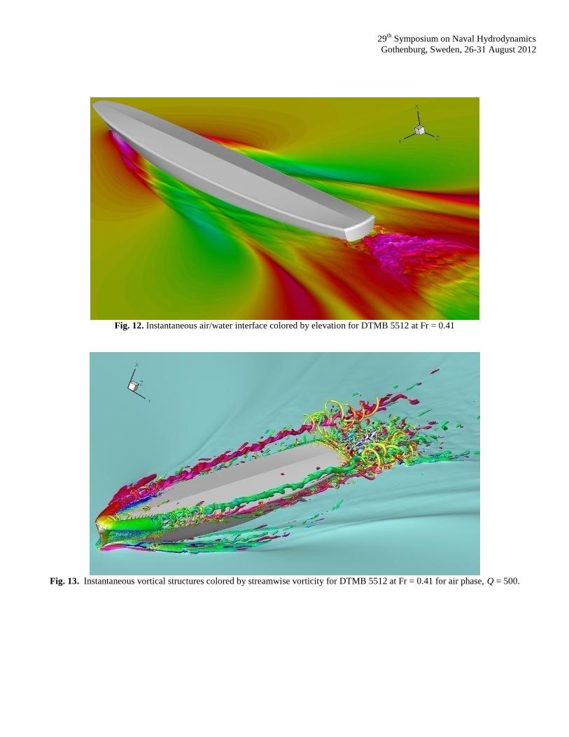
29th
Symposium on Naval Hydrodynamics
Gothenburg, Sweden, 26-31 August 2012
Fig. 12. Instantaneous air/water interface colored by elevation for DTMB 5512 at Fr = 0.41
Fig. 13. Instantaneous vortical structures colored by streamwise vorticity for DTMB 5512 at Fr = 0.41 for air phase, Q = 500.
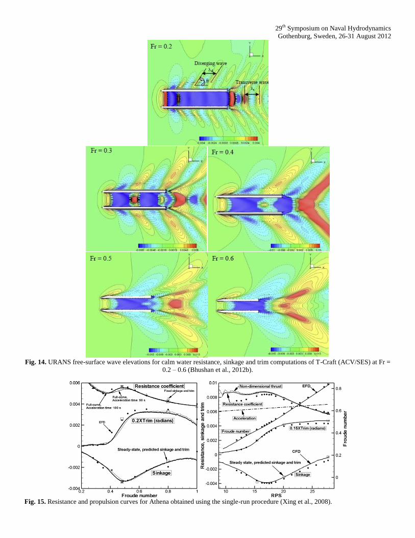
29th
Symposium on Naval Hydrodynamics
Gothenburg, Sweden, 26-31 August 2012
Fig. 14. URANS free-surface wave elevations for calm water resistance, sinkage and trim computations of T-Craft (ACV/SES) at Fr =
0.2 – 0.6 (Bhushan et al., 2012b).
Fig. 15. Resistance and propulsion curves for Athena obtained using the single-run procedure (Xing et al., 2008).
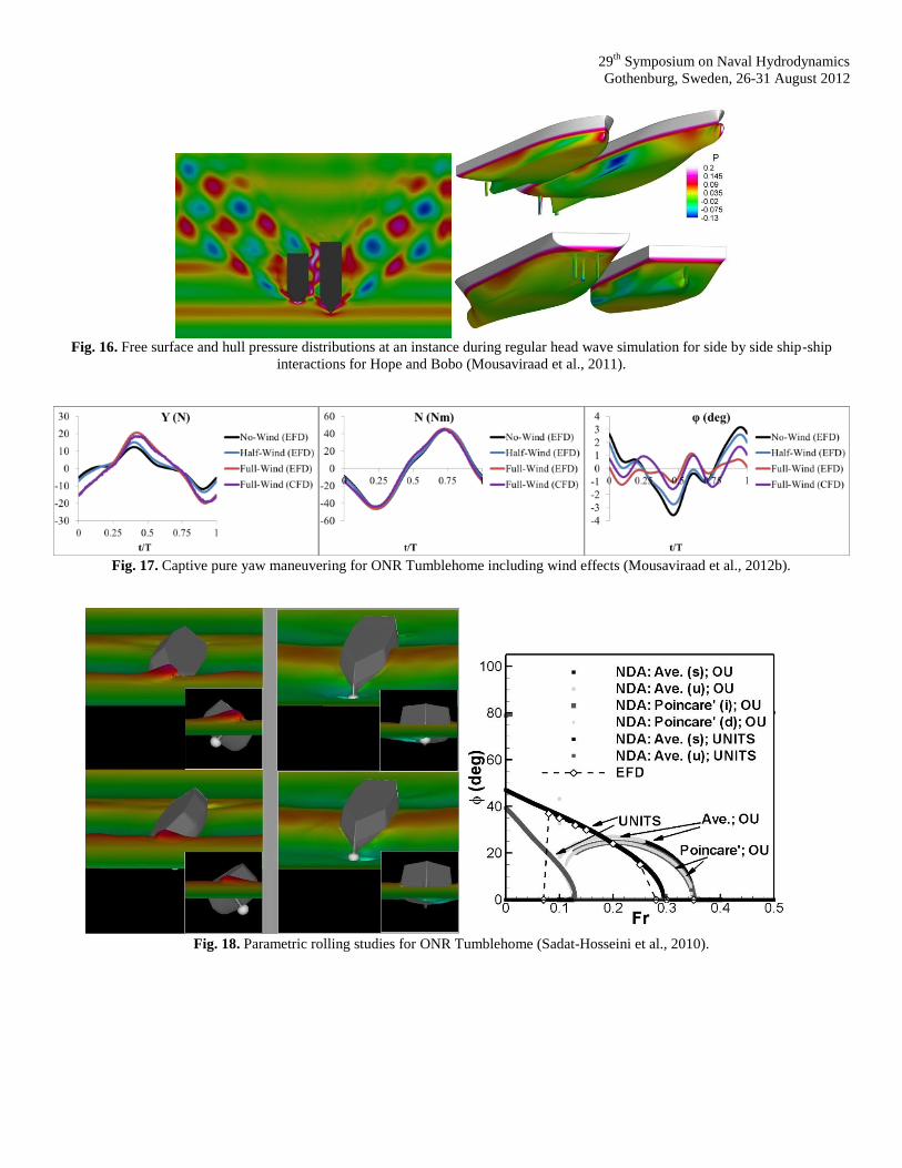
29th
Symposium on Naval Hydrodynamics
Gothenburg, Sweden, 26-31 August 2012
Fig. 16. Free surface and hull pressure distributions at an instance during regular head wave simulation for side by side ship-ship
interactions for Hope and Bobo (Mousaviraad et al., 2011).
Fig. 17. Captive pure yaw maneuvering for ONR Tumblehome including wind effects (Mousaviraad et al., 2012b).
Fig. 18. Parametric rolling studies for ONR Tumblehome (Sadat-Hosseini et al., 2010).
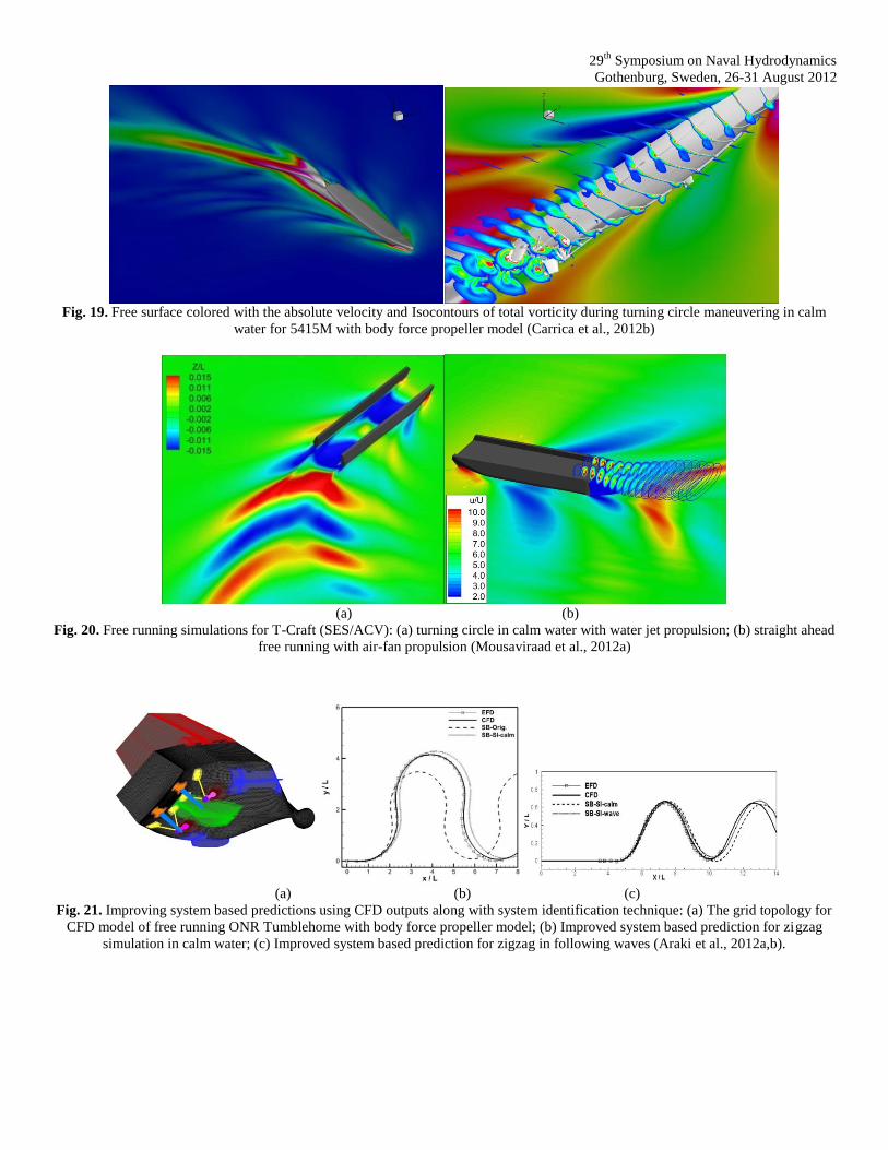
29th
Symposium on Naval Hydrodynamics
Gothenburg, Sweden, 26-31 August 2012
Fig. 19. Free surface colored with the absolute velocity and Isocontours of total vorticity during turning circle maneuvering in calm
water for 5415M with body force propeller model (Carrica et al., 2012b)
(a) (b)
Fig. 20. Free running simulations for T-Craft (SES/ACV): (a) turning circle in calm water with water jet propulsion; (b) straight ahead
free running with air-fan propulsion (Mousaviraad et al., 2012a)
(a) (b) (c)
Fig. 21. Improving system based predictions using CFD outputs along with system identification technique: (a) The grid topology for
CFD model of free running ONR Tumblehome with body force propeller model; (b) Improved system based prediction for zigzag
simulation in calm water; (c) Improved system based prediction for zigzag in following waves (Araki et al., 2012a,b).
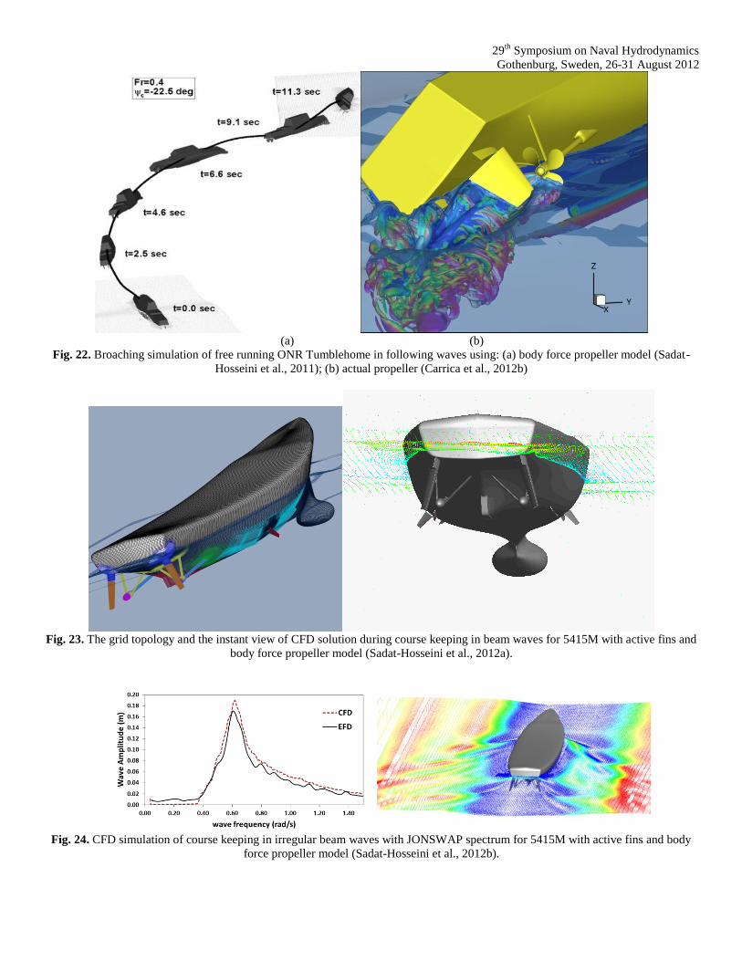
29th
Symposium on Naval Hydrodynamics
Gothenburg, Sweden, 26-31 August 2012
(a) (b)
Fig. 22. Broaching simulation of free running ONR Tumblehome in following waves using: (a) body force propeller model (Sadat-
Hosseini et al., 2011); (b) actual propeller (Carrica et al., 2012b)
Fig. 23. The grid topology and the instant view of CFD solution during course keeping in beam waves for 5415M with active fins and
body force propeller model (Sadat-Hosseini et al., 2012a).
Fig. 24. CFD simulation of course keeping in irregular beam waves with JONSWAP spectrum for 5415M with active fins and body
force propeller model (Sadat-Hosseini et al., 2012b).
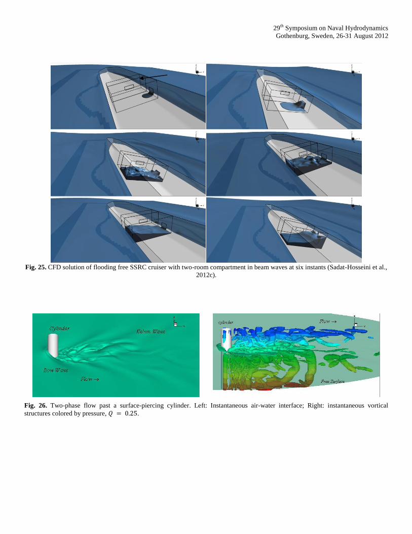
29th
Symposium on Naval Hydrodynamics
Gothenburg, Sweden, 26-31 August 2012
Fig. 25. CFD solution of flooding free SSRC cruiser with two-room compartment in beam waves at six instants (Sadat-Hosseini et al.,
2012c).
Fig. 26. Two-phase flow past a surface-piercing cylinder. Left: Instantaneous air-water interface; Right: instantaneous vortical
structures colored by pressure, .
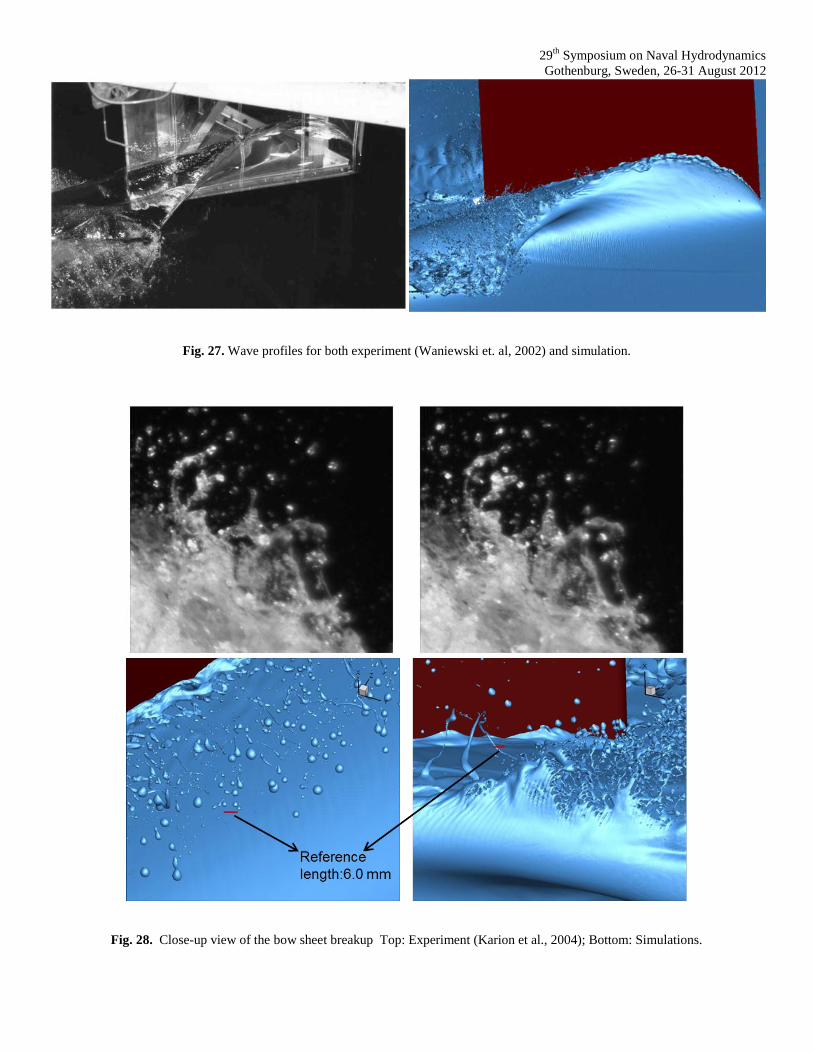
29th
Symposium on Naval Hydrodynamics
Gothenburg, Sweden, 26-31 August 2012
Fig. 27. Wave profiles for both experiment (Waniewski et. al, 2002) and simulation.
Fig. 28. Close-up view of the bow sheet breakup Top: Experiment (Karion et al., 2004); Bottom: Simulations.
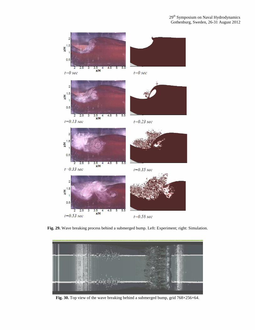
29th
Symposium on Naval Hydrodynamics
Gothenburg, Sweden, 26-31 August 2012
Fig. 29. Wave breaking process behind a submerged bump. Left: Experiment; right: Simulation.
Fig. 30. Top view of the wave breaking behind a submerged bump, grid 768×256×64.
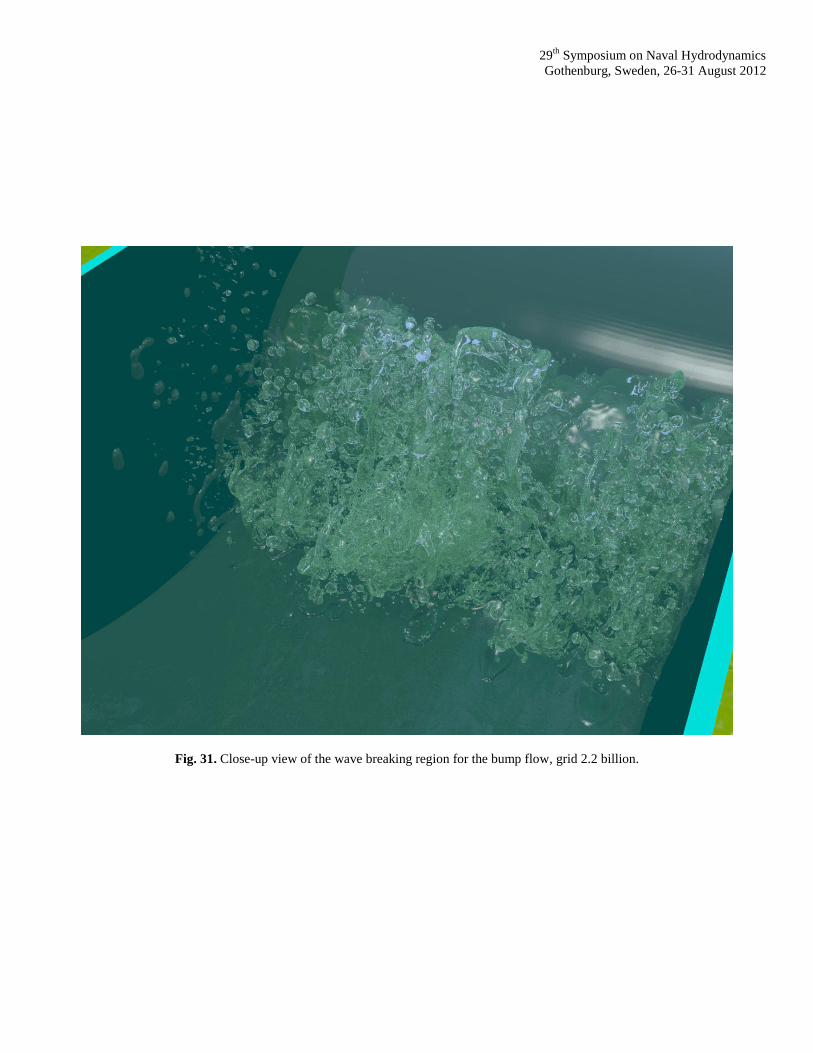
29th
Symposium on Naval Hydrodynamics
Gothenburg, Sweden, 26-31 August 2012
Fig. 31. Close-up view of the wave breaking region for the bump flow, grid 2.2 billion.
Recommended