
Master Thesis
Compressive sensing for IoT-driven
reliable video surveillance
June 2016
Student: Supervisor:
Laetitia REVERSEAU Daniel E. LUCANI
1
Department of Electronic Systems
Fredrik Bajers Vej 7
DK-9220 Aalborg O
https://es.aau.dk
Title:
Compressive sensing for IoT-
driven reliable video
surveillance
School and Study Board:
School of Information and
Communication Technology
(SICT)
Programme:
Network and Distributed
Systems
Student name:
Laetitia Reverseau
Project group:
16gr1026
Project Supervisor:
Daniel E. Lucani Roetter
Project Period:
Spring Semester 2016
Date of Completion:
June 2016
Abstract:
In recent years, there has been a huge explosion in
the variety of sensors and in the dimensionality of the data
the sensors required, in all kinds of applications from
medical imaging to video surveillance. As a result, a
‘deluge of data’ is occuring in many of these applications.
In 2007 according to the International Data Corporation
[1], the total amount of information being created by the
world sensors began to exceed the amount of storage.
Furthermore, transmitting all data to the cloud for further
processing is, in many applications, costly and
unnecessary. For example, providing sensor data in a farm
or video surveillance would benefit from local storage and
pre-processing before upload to the cloud. ‘Compressive
sampling’ or ‘compressed sensing’ (CS) constitutes an
appealing pre-processing technique that samples sparse
signals in a much more efficient way than the established
Nyquist density sampling theory. Since many natural
signals are sparse, CS allows for simple sensors to sample
at low rate to later use advanced algorithms for
reconstruction at the receiver.
This thesis studies how to apply compressive sensing for
video surveillance applications considering spatial
correlation within a picture (frame) and across pictures
(frames) from multiple cameras. The thesis relies on
multiple images analysed with standard metrics (e.g.,
PSNR, SSIM) and pre-processing techniques to determine
good thresholds for the early measurements and storage
requirements per image. Given our results, taking 1000
samples from an image originally containing 2500 pixels
would be enough to have a good image reconstruction,
while 300 to 500 samples will be enough to detect the
edges and contours of the image, which provides key
information for video surveillance. Finally, we propose
several mechanisms to bring together images from
multiple cameras with potential overlap and study the
effect of asymmetric sampling across the cameras.

Acknowledgments 2
Acknowledgments
I would first like to thank my thesis advisor Dr. Daniel E. Lucani of
the School of Information and Communication Technology at Aalborg
University. He found the time to help me when I ran into a trouble spot or
had a question about my work. He also made sure everything was going
well apart from the completion of my thesis.
I would also like to acknowledge the department secretary, director,
and members for welcoming and helping me, especially at the beginning of
my semester.
I also wish to thank the other people working in the lab for their
kindness and for making me feel comfortable joining them.
Finally, I must express my very profound gratitude to my family for
providing me with unfailing support and continuous encouragement
throughout my years of study and in every aspect of my life. This
accomplishment would not have been possible without them. Thank you.

Table of contents 3
Table of contents
Acknowledgments ..................................................................................................... 2
Table of contents ....................................................................................................... 3
List of figures ............................................................................................................ 4
Acronyms .................................................................................................................. 6
Introduction ............................................................................................................... 7
1.1. The video surveillance market .................................................................. 7
1.2. Network Coding ........................................................................................ 8
1.3. Compressive Sensing .............................................................................. 10
1.4. Our proposition ....................................................................................... 11
State of the art in Network coding and Cloud computing ....................................... 12
2.1. Coding for storage ................................................................................... 12
2.2. Video processing in the Cloud ................................................................ 20
State of the art in Compressive Sensing .................................................................. 25
3.1. Compressive Sensing .............................................................................. 25
3.2. Coupling of Network Coding and Compressive Sensing ....................... 30
Problem Statement .................................................................................................. 32
4.1. Importance of video surveillance ............................................................ 32
4.2. Architecture of video surveillance systems............................................. 33
4.3. Requirements and stakes in video analytics ............................................ 35
Single image processing: Compressive Sensing implementation ........................... 36
5.1. Simple Compressed Sensing examples ................................................... 36
5.2. PSNR calculation .................................................................................... 38
5.3. The limitation of PSNR and an alternative: SSIM .................................. 41
5.4. Edge detection ......................................................................................... 45
5.5. Conclusion .............................................................................................. 50
Multiple image processing: Image stitching ........................................................... 51
6.1. Feature Based Image Stitching ............................................................... 51
6.2. Image stitching and Compressive Sensing .............................................. 61
6.3. Conclusion .............................................................................................. 64
Conclusion and future work .................................................................................... 65
Sources .................................................................................................................... 67
List of figures 4
List of figures
Introduction
1.1. Average data generated by new surveillance cameras
shipped globally ........................................................................ 7
1.2. A classical network coding example ......................................... 9
State of the art in Network coding and video transmission
2.1. Multicast tree example ............................................................ 14
2.2. Example showing that 50% redundancy cannot guarantee
100% reliability if any node disconnects ................................ 15
2.3. Example showing that using coding 50% redundancy can
guarantee 100% reliability if any node disconnects ............... 15
2.4. Example of the repair process when using a (6, 4) MDS
code ......................................................................................... 17
2.5. How cloud computing works ................................................... 21
2.6. Split&Merge architecture deployed on a public Cloud
infrastructure (Amazon Web Services) ................................... 23
State of the art in Compressive Sensing
3.1. Several representations of a signal in different basis ............. 29
Problem Statement
4.1. Standard digital data acquisition approach .......................... 35
Single image processing: Compressive Sensing implementation
5.1. Compressive measurement process and matrix product
Θ= ՓΨ .................................................................................... 36
5.2. Display of the solutions to y=Θ.s. Basis pursuit solution in
red, least squares solution in blue .......................................... 37
5.3. Loops for the least squares and basis pursuit
reconstructions ........................................................................ 38
5.4. Compressive sensing example ................................................ 38
5.5. Evolution of the PSNR in function of the number of random
measurements M from 100 to 2500 ......................................... 39
5.6. Example showing that PSNR is a good measure for
comparing restoration results for the same image, but
meaningless between different images .................................... 41

List of figures 5
5.7. SSIM values for different images reconstructed with 100 to
2500 measurements ................................................................. 44
5.8. SSIM values for CS images with and without edge detection . 46
5.9. Comparison of different edge detection filters: Canny,
Prewitt, Sobel, Roberts, Laplacian of Gaussian ..................... 48
5.10. SSIM index and PSNR values for different edge detection
methods ................................................................................... 49
Multiple image processing: Image stitching
6.1. Image stitching – horizontal shift ........................................... 54
6.2. Image stitching – vertical shift ................................................ 54
6.3. Image stitching – tilt ............................................................... 55
6.4. Image stitching – 3 input images ............................................ 55
6.5. Street image stitching – 2 images ........................................... 56
6.6. Street image stitching – 3 images ........................................... 56
6.7. Street image stitching – Distortion because of too strong
horizontal shift ........................................................................ 57
6.8. Region of bad pixels and corrected images ............................ 59
6.9. Result of the pixel-correction methods ................................... 60
6.10. CS image stitching for different sample rates ......................... 62
6.11. PSNR values between simple image stitching and CS image
stitching ................................................................................... 63
6.12. “Inverse butterfly”scheme ...................................................... 64

Acronyms 6
Acronyms
CNC Compressive Network coding
CPU Central Processing Unit
CS Compressive Sensing / Compressed Sampling
FEC Forward Error Correction
IoT Internet of Things
IP Internet Protocol
IT Information Technology
LoG Laplacian of Gaussian
MDS Maximum Distance Separable
MSE Mean-Squared Error
NC Network coding
NVR Network Video Recorder
PSNR Peak to Signal Noise Ratio
RLNC Random Linear Network coding
SSIM Structural Similarity Index Measurement
WSN Wireless Sensor Network

Introduction 7
Chapter 1
Introduction
1.1. The video surveillance market
The security market is all the time adopting new technologies to
guarantee protection to people and their property. The world market for
video surveillance solutions is experimenting a wide digitalization to reach
the critical mass, and has experienced a strong growth in recent years, which
is forecast to continue at rate of 12.4% per year to $25.6 billion in 2018 [2].
The ‘deluge of data’ continues to increase with the proliferation of
always higher resolution cameras, reaching 566 petabytes of data produced
in one day by all the video surveillance cameras installed worldwide in 2015
– as announced in IHS new survey carried out in early 2016 [3].
Figure 1.1: Average data generated by new surveillance cameras shipped
globally. [3]
Video surveillance cameras produce a huge amount of high
resolution data, which becomes a challenge to compute and store. Thus,
enterprise storage systems dedicated to video surveillance need to have a
larger throughput capacity. Previously separated, IT and security have
finally joined forces to meet the increase of surveillance storage demands.
However, past approaches will no longer be sufficient and those demands
may force end-users to change their storage solutions.
Introduction 8
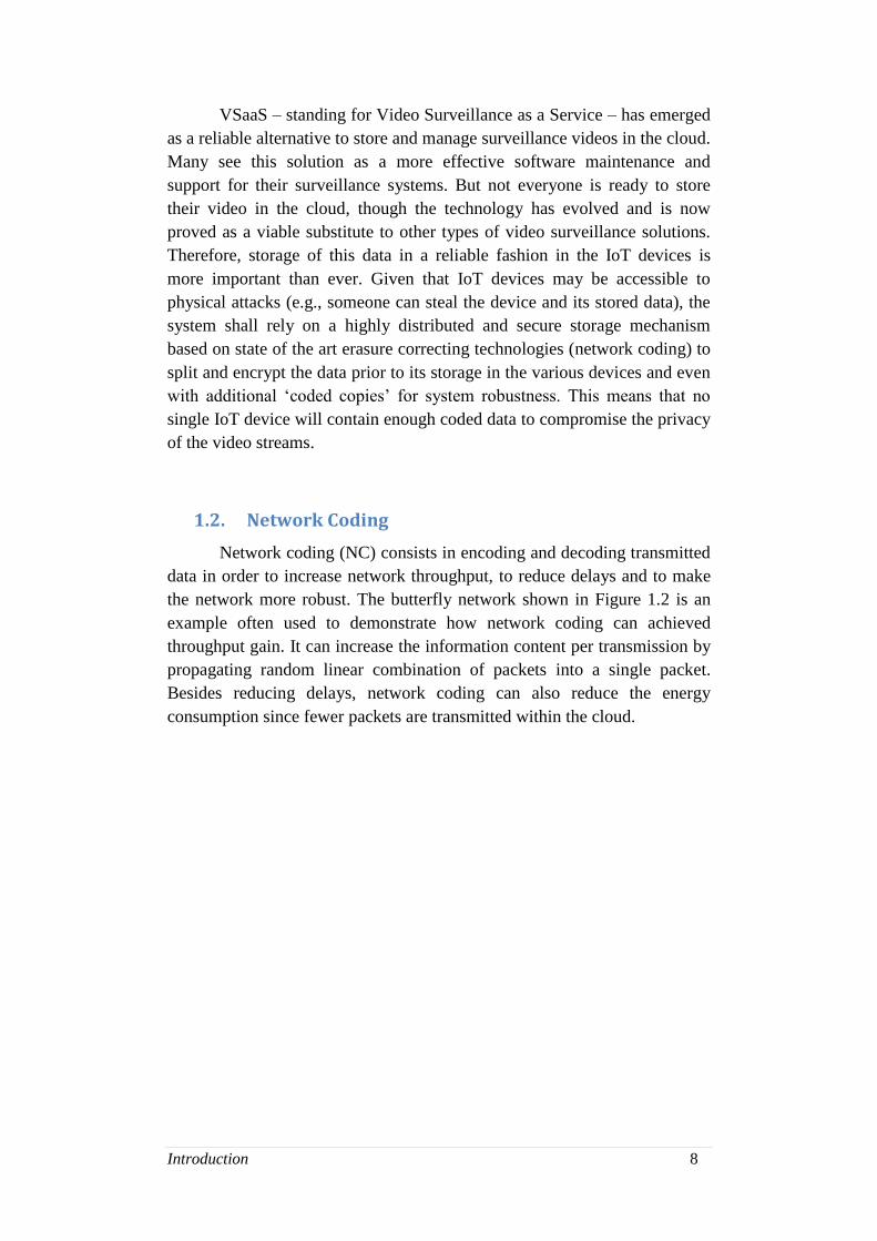
VSaaS – standing for Video Surveillance as a Service – has emerged
as a reliable alternative to store and manage surveillance videos in the cloud.
Many see this solution as a more effective software maintenance and
support for their surveillance systems. But not everyone is ready to store
their video in the cloud, though the technology has evolved and is now
proved as a viable substitute to other types of video surveillance solutions.
Therefore, storage of this data in a reliable fashion in the IoT devices is
more important than ever. Given that IoT devices may be accessible to
physical attacks (e.g., someone can steal the device and its stored data), the
system shall rely on a highly distributed and secure storage mechanism
based on state of the art erasure correcting technologies (network coding) to
split and encrypt the data prior to its storage in the various devices and even
with additional ‘coded copies’ for system robustness. This means that no
single IoT device will contain enough coded data to compromise the privacy
of the video streams.
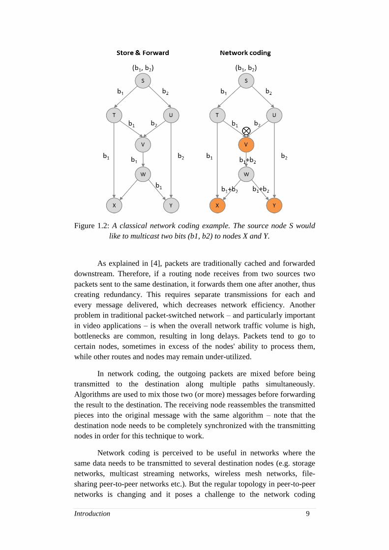
1.2. Network Coding
Network coding (NC) consists in encoding and decoding transmitted
data in order to increase network throughput, to reduce delays and to make
the network more robust. The butterfly network shown in Figure 1.2 is an
example often used to demonstrate how network coding can achieved
throughput gain. It can increase the information content per transmission by
propagating random linear combination of packets into a single packet.
Besides reducing delays, network coding can also reduce the energy
consumption since fewer packets are transmitted within the cloud.
Introduction 9
Figure 1.2: A classical network coding example. The source node S would
like to multicast two bits (b1, b2) to nodes X and Y.
As explained in [4], packets are traditionally cached and forwarded
downstream. Therefore, if a routing node receives from two sources two
packets sent to the same destination, it forwards them one after another, thus
creating redundancy. This requires separate transmissions for each and
every message delivered, which decreases network efficiency. Another
problem in traditional packet-switched network – and particularly important
in video applications – is when the overall network traffic volume is high,
bottlenecks are common, resulting in long delays. Packets tend to go to
certain nodes, sometimes in excess of the nodes' ability to process them,
while other routes and nodes may remain under-utilized.
In network coding, the outgoing packets are mixed before being
transmitted to the destination along multiple paths simultaneously.
Algorithms are used to mix those two (or more) messages before forwarding
the result to the destination. The receiving node reassembles the transmitted
pieces into the original message with the same algorithm – note that the
destination node needs to be completely synchronized with the transmitting
nodes in order for this technique to work.
Network coding is perceived to be useful in networks where the
same data needs to be transmitted to several destination nodes (e.g. storage
networks, multicast streaming networks, wireless mesh networks, file-
sharing peer-to-peer networks etc.). But the regular topology in peer-to-peer
networks is changing and it poses a challenge to the network coding
Introduction 10
technique because it complicates network synchronization. Plus, the data
may take a lot of time to be decoded.
This distribution method can increase the effective capacity of a
network by minimizing the number and severity of bottlenecks. The
difference with traditional methods is even more significant when network
traffic volume is near the maximum capacity obtainable with traditional
routing. Overall, network coding can increase the efficiency in large
networks, but high overhead costs may make them less manageable for
smaller networks.
Regarding video streams, network codes should be selected in order
to maximize both the video quality and the network throughput. The video
streaming community studies in depth the unequal importance of video
packets. On the other hand, the network coding community has proved that
mixing different information flows can increase throughput in multicast
networks. In [5], video-aware opportunistic network coding schemes try to
consider both aspects – namely the decodability of network codes by several
receivers, and the distortion values and playout deadlines of video packets.
But transmitting all data to the cloud for further processing is, in
many applications, costly and unnecessary. For example, providing sensor
data in a farm or video surveillance would benefit from local storage and
pre-processing before upload to the cloud. That is why some techniques
have emerged to sample or compress data as most of the data is redundant.
1.3. Compressive Sensing
Compressive sensing (CS) is also referred as compressed sensing,
compressive sampling or sparse sampling. It is a signal processing method
used to efficiently acquire and reconstruct a signal by finding the sparsest
solution to underdetermined linear systems.
The core of signal processing is based on the Shannon/Nyquist
theorem: a continuous time-signal sampled at twice its highest frequency,
can be recovered exactly. Very recently, an alternative theory has emerged,
known as ‘compressive sensing’. By using nonlinear recovery algorithms
(based on convex optimization of the l1-norm described more in depth in
Chapter 2), super-resolved signals and images can be reconstructed from
what appears to be highly incomplete data. For example, CCD digital
cameras (charge coupled device) take pictures with around 10 million
pixels. In the end, about 5% of the initial measurements will be stored
because the other 95% give redundant information. So instead of acquiring
and then throwing away most of the data, the idea of CS is to directly get
Introduction 11
only the informative part of the signal. Thus, compressive sensing shows us
how data compression can be implicitly incorporated into the data
acquisition process, and gives a new perspective for many applications
including analog-to-digital conversion.
This is a pre-processing step in the process of IoT-video surveillance
storage, which can be divided into capture of video surveillance, storage of
this data in a reliable fashion in the IoT devices, and allowing access and
playback by users. This project will focus specifically on compressive
sensing for data compression as part of an efficient protocol that could
automatically translate analog data into already compressed digital form to
be later computed for reconstruction.
Compressed sensing could have important implications, such as new
data acquisition protocols that translate analog information into digital form
with fewer sensors than what was considered necessary. Processes for
simultaneous signal acquisition and compression could be improved with
this new sampling theory.
1.4. Our proposition
As video surveillance cameras have higher and higher resolution, the
challenge of reducing the amount of data to be stored is more important than
ever. We considered two main cases: a scene recovered by a single camera,
and a zone covered by multiple cameras.
In the first case, we worked on applying compressive sensing within
a picture while maintaining a good image quality. We evaluated the quality
of the compressed images with two different techniques: the PSNR and the
SSIM index. Finally, we investigated the utility of applying edge detection
filters on CS images to get better results with fewer samples.
In the second case, as there is most likely some overlap between the
different devices to assure a full coverage of the area, we worked on how to
combine several images. We also considered the application of image
stitching besides compression. For this, we proposed three scenarios
depending on the order in which the transformations (compression and
stitching) were applied.
Even though we ran the different image processing methods locally
rather than dealing with cloud computing, we also included a state of the art
of video processing in the cloud since this concept is becoming ubiquitous
in the digital era we are living in and the resulting data deluge.
State of the art in Network coding and Cloud computing 12
Chapter 2
State of the art in Network coding and Cloud computing
2.1. Coding for storage
2.1.1. Erasure coding and Network coding for storage
Distributed storage aims at storing data over a long period of time
and in a reliable way. It uses a distributed collection of storage nodes which
may be individually unreliable. Erasure coding offers a good option to store
those data efficiently. It breaks the outgoing file of size M into k packets of
size M / k, and instead of storing n replicas of the fragments, n coded pieces
are produced using an encoder and a maximum distance separable (MDS)
code (n, k). Then, any set of k pieces of size M / k is enough to recover the
whole file, which makes the approach optimal in terms of
reliability/redundancy tradeoff [18, 20]. This technique is much more
reliable for the same amount of redundancy than simple replication [19].
Moreover, the system should no longer keep track of where the replicated
pieces are stored. Instead it should only guarantee that enough different
pieces are available at any time.
One of the most frequently used digital error control codes are Reed-
Solomon codes, especially for the redundancy in data storage systems.
The use of traditional MDS codes raises new difficulties. When a
node fails or disconnects from the network, the system must compensate the
redundancy lost with that node. With replication, the piece lost is simply
copied from another node in the network, without any repair overhead i.e. to
repair k bits, only k bits are transmitted over the network. On the other hand,
codes like Reed-Solomon first need to decode the whole file to be able to
generate new coded pieces. Thus, repairing a fragment of size M / k requires
a minimum bandwidth of M, i.e. at least the whole file must be transferred
over the network every time the system builds new redundancy.
Network coding appears as a solution to this difficulty. This recent
technique enables to generate erasure codes – also known as forward error
correction (FEC) codes – which allow repairing by transmitting the
information theoretic minimum over the network [18]. The most common
technique of network coding is Random Linear Network Coding (RLNC).
This technique, when used for file coding purpose, takes the original k
pieces of a file x1, x2,…, xk and creates n linear combination p1, p2,…, pn of
the same size called coded packets, where pj is:
State of the art in Network coding and Cloud computing 13
𝑝𝑗 = ∑ 𝒄𝒊,𝒋. 𝒙𝒊
𝑘
𝑖=1
(2-1)
𝒄𝒊,𝒋 are the coefficients chosen randomly and independently by
each node over a finite field, commonly the Galois Field i.e. of the form
GF(2m) – in general GF(2
8) is sufficient. These coefficients are then
appended to each coded packet, so receiver nodes will know how to recover
the source data. Similarly as in Reed-Solomon codes, any set of k linear
independent packets are enough to decode the file. Yet, an innovation of
network coding over Reed-Solomon codes is that it allows the recoding of
already-coded packets p1, p2,…pn , i.e. it is possible to generate new coded
packets p’ without decoding the whole file. p’ is:
𝑝′ = ∑ 𝑐𝑖 . 𝑝𝒊
𝑛
𝑖=1
(2-2)
As random combinations of the files are distributed among the peers
and cloud services instead of just raw data, network coding offers an
intrinsic level of security. The data remains private even when
“mischievous” peers are present in the network or when a cloud service gets
compromised by external agents. An eavesdropper would need to
compromise the whole system and gather enough coded packets in order to
be able to decode and “understand” the data.
At the same time, network coding has proven benefits in several
communication scenarios. In point-to-point communications, it allows to
repair packet losses in lossy channels. If there is an estimation of the packet
error probability, the transmitter can send extra coded packets. Since it is
not relevant to know which specific packets got lost, this does not require
extra feedback from the receiver. In multicast scenarios over lossy wireless
channels, when several nodes want to receive the same data, if the
transmitter broadcasts uncoded packets, then it will need to retransmit every
single lost packet. Due to the uncorrelated losses, many of these
retransmissions will be useful only for a few nodes. If coded packets are
sent instead, the information contained in the retransmitted packets might
benefit with high probability all the nodes that experienced losses.
By using network coding in a distributed storage system to manage
the storage and communications with a single code structure, this project
takes advantages of the benefits of that technology in the field of storage
State of the art in Network coding and Cloud computing 14
and wireless communications. This brings reliable multicast and higher data
transmission rates in lossy channels.
As underlined in [21], adapting network coding to robust video
transmission in wireless networks raises several challenges in terms of video
quality, bandwidth and delays. Indeed, wireless networks can suffer from
dynamic channel variations and interference in a shared medium. There are
different options to address these issues. One of them is to apply NC erasure
protection over the different channels, i.e. over uplink, downlink and
overhearing channels, especially in the context of video conferencing, live
surveillance or other live-video applications. Another solution is to assign
an unequal amount of forward error correction codes on different video
layers based on their importance. FEC gives the receiver the ability to
correct errors without needing a reverse channel to request retransmission of
data, but at the cost of a larger forward channel bandwidth. Another way to
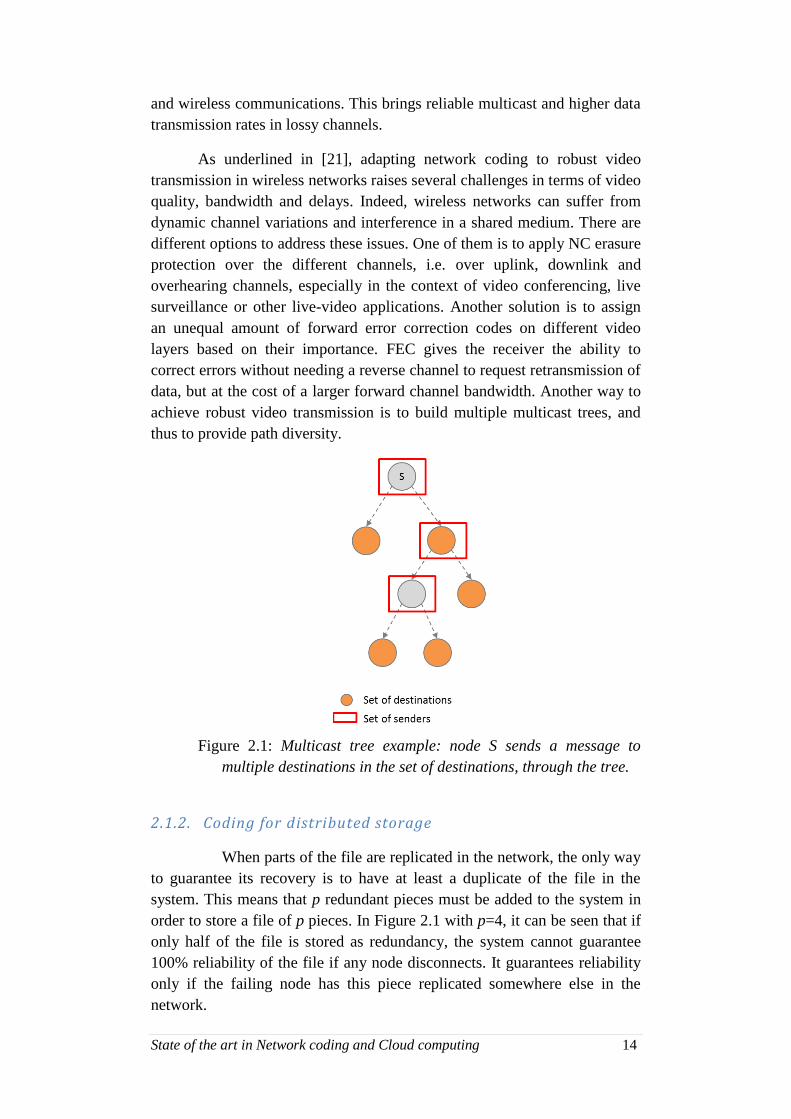
achieve robust video transmission is to build multiple multicast trees, and
thus to provide path diversity.
Figure 2.1: Multicast tree example: node S sends a message to
multiple destinations in the set of destinations, through the tree.
2.1.2. Coding for distributed storage
When parts of the file are replicated in the network, the only way
to guarantee its recovery is to have at least a duplicate of the file in the
system. This means that p redundant pieces must be added to the system in
order to store a file of p pieces. In Figure 2.1 with p=4, it can be seen that if
only half of the file is stored as redundancy, the system cannot guarantee
100% reliability of the file if any node disconnects. It guarantees reliability
only if the failing node has this piece replicated somewhere else in the
network.
State of the art in Network coding and Cloud computing 15
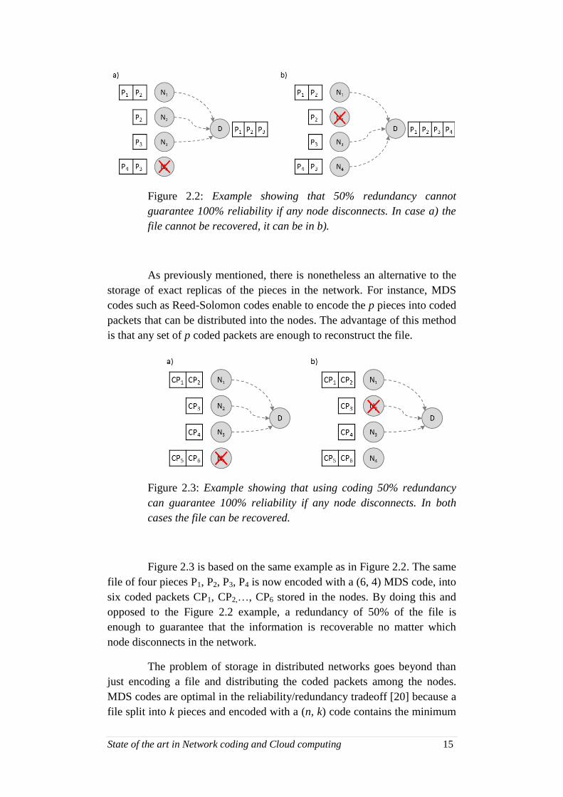
Figure 2.2: Example showing that 50% redundancy cannot
guarantee 100% reliability if any node disconnects. In case a) the
file cannot be recovered, it can be in b).
As previously mentioned, there is nonetheless an alternative to the
storage of exact replicas of the pieces in the network. For instance, MDS
codes such as Reed-Solomon codes enable to encode the p pieces into coded
packets that can be distributed into the nodes. The advantage of this method
is that any set of p coded packets are enough to reconstruct the file.
Figure 2.3: Example showing that using coding 50% redundancy
can guarantee 100% reliability if any node disconnects. In both
cases the file can be recovered.
Figure 2.3 is based on the same example as in Figure 2.2. The same
file of four pieces P1, P2, P3, P4 is now encoded with a (6, 4) MDS code, into
six coded packets CP1, CP2,…, CP6 stored in the nodes. By doing this and
opposed to the Figure 2.2 example, a redundancy of 50% of the file is
enough to guarantee that the information is recoverable no matter which
node disconnects in the network.
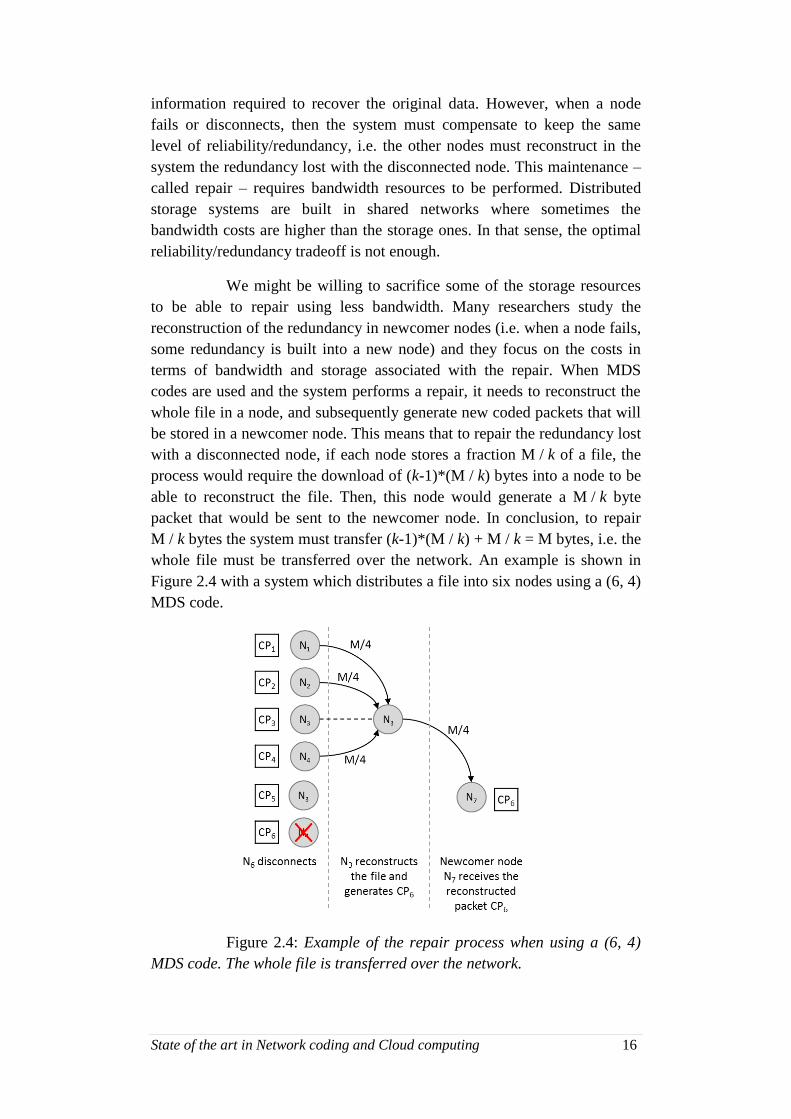
The problem of storage in distributed networks goes beyond than
just encoding a file and distributing the coded packets among the nodes.
MDS codes are optimal in the reliability/redundancy tradeoff [20] because a
file split into k pieces and encoded with a (n, k) code contains the minimum
State of the art in Network coding and Cloud computing 16
information required to recover the original data. However, when a node
fails or disconnects, then the system must compensate to keep the same
level of reliability/redundancy, i.e. the other nodes must reconstruct in the
system the redundancy lost with the disconnected node. This maintenance –
called repair – requires bandwidth resources to be performed. Distributed
storage systems are built in shared networks where sometimes the
bandwidth costs are higher than the storage ones. In that sense, the optimal
reliability/redundancy tradeoff is not enough.
We might be willing to sacrifice some of the storage resources
to be able to repair using less bandwidth. Many researchers study the
reconstruction of the redundancy in newcomer nodes (i.e. when a node fails,
some redundancy is built into a new node) and they focus on the costs in
terms of bandwidth and storage associated with the repair. When MDS
codes are used and the system performs a repair, it needs to reconstruct the
whole file in a node, and subsequently generate new coded packets that will
be stored in a newcomer node. This means that to repair the redundancy lost
with a disconnected node, if each node stores a fraction M / k of a file, the
process would require the download of (k-1)*(M / k) bytes into a node to be
able to reconstruct the file. Then, this node would generate a M / k byte
packet that would be sent to the newcomer node. In conclusion, to repair
M / k bytes the system must transfer (k-1)*(M / k) + M / k = M bytes, i.e. the
whole file must be transferred over the network. An example is shown in
Figure 2.4 with a system which distributes a file into six nodes using a (6, 4)
MDS code.
Figure 2.4: Example of the repair process when using a (6, 4)
MDS code. The whole file is transferred over the network.
State of the art in Network coding and Cloud computing 17
This reliability/redundancy tradeoff in this kind of repairs has
been recently studied ([18, 20] among others), concluding that by using
network coding it is possible to generate codes capable of reducing the
bandwidth required for the repair. Dimakis et al. [18] found that it was
possible to find the optimal curve describing the tradeoff storage-bandwidth:
such curve can be achieved using network coding.
2.1.3. Random Linear Network Coding
Random Linear Network Coding (RLNC) is a technique used to
improve network performance in terms of throughput, scalability, efficiency
and also for resilience to attacks and eavesdropping. Contrary to the
deterministic Linear Network Coding, RLNC is a distributed scheme that
circumvents the constraint of knowing the global network topology to find
the coding coefficients. RLNC has a probabilistic success rate that increases
exponentially with field size.
In RLNC a coded packet pj is generated producing linear
combinations of the original k data pieces x1, x2,…xk such as:
𝑝𝑗 = ∑ 𝒄𝒊,𝒋. 𝒙𝒊
𝑘
𝑖=1
(2-3)
Each coded packet can be considered as a k-variable linear
equation. Since addition and multiplication are performed over the finite
field, then the size of the coded packets will be the same size as the original
pieces. Also, it is possible to use all the known linear algebra tools
(matrices, Gauss-Jordan elimination…) to solve linear equations. Thus, a
decoder will need only k linear independent packets to be able to reconstruct
the whole data. The equation 2-4 is a different way from 2-3 to show the
link between the coded packets pi, the coding coefficients cij and the original
pieces xi.
[
𝑝1
⋮𝑝𝑛
] = [
𝑐11 𝑐12 ⋯ 𝑐1𝑘
⋮ ⋱ ⋮𝑐𝑛1 𝑐𝑛2 ⋯ 𝑐𝑛𝑘
]. [
𝑥1
⋮𝑥𝑘
]
(2-4)
Metadata will need to be included with the encoded packets, so
receiver nodes will know how to recover the source data. The coefficients
used to generate each pi constitute a vector known as the coding vector
which is added as an overhead in packet transmission. The size of this
State of the art in Network coding and Cloud computing 18
coding vector in bytes depends on the size of the finite field and on the
number of original pieces used, known as generation size.
For example, to transfer an image of 2MB, it is split into 500
pieces of 4KB each. The generation size is then k=500. Each coded packet is
generated making linear combinations of vector. If the size of the finite field
is q=2, i.e. GF(2)={0,1}, the size of the overhead due to coding vectors will
be 𝑘. log2(𝑞), that is 500 bits added at the end of each coded packet. This
means that each pi contains 4KB of information and a 500-bit overhead. The
overhead corresponds to 1.25% of the transferred packet. When the symbol
size gets bigger, the overhead due to the coding vector becomes negligible.
There is another type of overhead in RLNC due to linear
dependency. Since the coefficients are chosen randomly, the probability of
generating linear dependent packets is a function of the generation size and
the field size q. Ho et al. [22] bounded the probability of this error
𝑃 ≤ (1- 𝑟
|𝑞| )
η
for q > r, where r is the number of receivers, and η is the number
of links involved in the graph. It can be shown that the probability of
randomly selecting a non-admissible network code diminishes exponentially
with code length.
The overhead due to linear dependencies occurs because linear
dependent packets do not provide new information to the decoder, so it
becomes necessary to send extra packets. The bigger the size of the field is,
the smaller the probability of generating linear dependent packets, but the
higher the overhead due to the size of coding vectors. The computational
complexity associated with encoding and decoding increases when the
generation size becomes bigger. For that reason, if the system needs to
encode or decode a big file it first divides it into blocks and then performs
the encoding operations over these blocks of a more manageable size.
2.1.4. RLNC in video transmission
Applying RLNC to video streaming in erasure network presents
both advantages and drawbacks.
On one hand, rank deficiency problem has a negative impact on
video quality and erasure coding performance. Indeed, if the number of lost
packets is higher than the redundancy rank of the generator matrix, the
video decoder is lacking useful data blocks and cannot invert the source file
properly. Thus, the RLNC rank deficiency issue must be addressed to enable
State of the art in Network coding and Cloud computing 19
effective error concealment and obtain high quality videos. Wang et al [21]
listed some solutions to the rank deficiency problem such as an error-
resilient RLNC method, which guarantees the recovery of the source
packets if the number of lost packets does not exceed the minimum distance
provided by the rank-metric code. Another solution would be the
concatenation of two known coding methods – low-density parity-check
code (LDPC) with RLNC – which arrange the source packets by priority
and code them with a priority error transmission (PET) scheme. This
guarantees that the most important n packets can be decoded at the
destination as long as n RLNC packets are received. Finally, the third
solution mentioned is to combine video interleaving (VI) with network
coding.
On the other hand, by releasing new independent packets in the
intermediate nodes of the network, RLNC increases error-resilience. When
pure RLNC encoding is used at the source and intermediate nodes rather
than forward error correction (FEC) codes [21], both erasure protection and
coding delay are improved. Also note that erasure channel codes such as
Reed-Solomon previously mentioned used to recover data from erasures are
not as simple on video files since the decoding delays can be very
“expensive” for video quality.
Seferoglu et al. [5] proposed a scheme which takes into account
both the decodability of network codes by several receivers and the
importance and deadlines of video packets. At the intermediate nodes, new
packets are generated by applying the XOR operator on video packets
selected from different streams according to their contribution to the overall
quality. The NC codes are generated depending on the priority and
emergency of these packets. Receiving nodes listen to the neighboring
transmissions and store overhead packets for future decoding. This
introduces storage overhead on the receivers. Moreover, the neighbor nodes
need to exchange and update the stored content with each other, which
necessitates extra communication in the network. Their simulation results
showed that their schemes significantly improved both video quality and
throughput.
More generally, network coding methods can improve the
throughput of data multicast while generating rateless erasure codes, i.e.
codes that do not exhibit a fixed code rate. However, it disables video error
concealment and may cause error propagation, resulting in degraded video
quality but some solutions have been proposed to address these issues.
State of the art in Network coding and Cloud computing 20
2.2. Video Processing in the Cloud
2.2.1. The Internet of Things
It is estimated that by 2020 there will be 50 billion of jacks
connected to the Internet and estimated by the U.S. Census Bureau that the
world population will reach 7.6 billion at that time. That means that for
every person on Earth there would be 6.6 objects connected to the Internet,
with billions of sensors taking information from real physical objects and
uploading it on the Internet. This world constantly changing all around
because of these sensors and the Internet is called the Internet of Things
(IoT). The latest version of Internet Protocol – IPv6 – creates more potential
IP addresses than there are atoms on the surface of the Earth. We are going
to live in a world completely filled with sensors and data reacting to us,
changing every moment depended upon our needs. It is altering reality as
we know it, and it is all regulated by the Internet of Things. Gartner [30]
estimated that the IoT will include 26 billion devices by 2020. Its
deployment will generate large amounts of data to be computed and stored.
Cloud services appear to be one of the solutions to address the storage
management issue.
2.2.2. Cloud computing and storage
Cloud storage is one of the most common methods used nowadays to
store data from video surveillance cameras.
The term “cloud computing” comes from the fact that the data and
applications are on a cloud of Web servers. In a cloud computing system,
the computer network handles the running of applications instead of local
computers. It results in a significant workload shift and a decrease of hard-
and software demands from the users. Usually, each application has its own
dedicated server. But as a server is likely to break down, a cloud computing
system needs to store a copy of all its clients’ information in backup servers
or other devices. Considering the Internet widespread, the increasing
demand of bandwidth, broadband and mobility for end-users, cloud
computing has become ubiquitous in today’s digital era, from consumers to
businesses.
State of the art in Network coding and Cloud computing 21
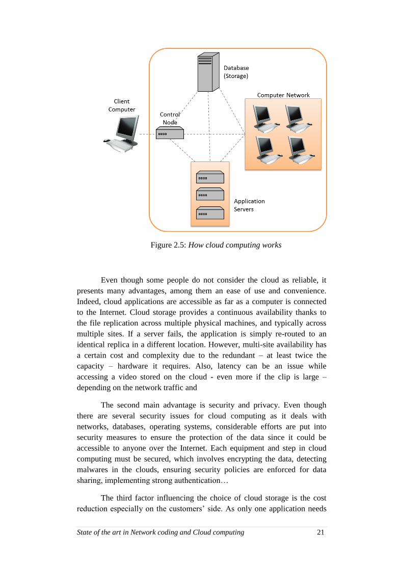
Figure 2.5: How cloud computing works
Even though some people do not consider the cloud as reliable, it
presents many advantages, among them an ease of use and convenience.
Indeed, cloud applications are accessible as far as a computer is connected
to the Internet. Cloud storage provides a continuous availability thanks to
the file replication across multiple physical machines, and typically across
multiple sites. If a server fails, the application is simply re-routed to an
identical replica in a different location. However, multi-site availability has
a certain cost and complexity due to the redundant – at least twice the
capacity – hardware it requires. Also, latency can be an issue while
accessing a video stored on the cloud - even more if the clip is large –
depending on the network traffic and
The second main advantage is security and privacy. Even though
there are several security issues for cloud computing as it deals with
networks, databases, operating systems, considerable efforts are put into
security measures to ensure the protection of the data since it could be
accessible to anyone over the Internet. Each equipment and step in cloud
computing must be secured, which involves encrypting the data, detecting
malwares in the clouds, ensuring security policies are enforced for data
sharing, implementing strong authentication…
The third factor influencing the choice of cloud storage is the cost
reduction especially on the customers’ side. As only one application needs
State of the art in Network coding and Cloud computing 22
to be hosted and maintained, it reduces the customers’ expenses. Plus, data
protection costs can also be cut since security is often intrinsic to the cloud
storage architecture. However, regarding video storage application, cloud
service could is likely to be much more expensive than a Network Video
Recorder system, because of the internet connection and the cloud storage
charges.
Network video recorders (NVR) – and respectively digital video
recorder (DVR) for analog cameras – are local systems used to manage,
view, and store surveillance videos from IP cameras. NVRs use the local
network infrastructure to send and receive surveillance data that can be
computed from a remote device.
2.2.3. Cloud Distributed Mechanisms
First developed at Google and now genericized, Map-Reduce is a
framework that aims to run various tasks in parallel. Its classic
implementation provides a single ‘master’ node, responsible for distributing
the tasks between the ‘worker’ nodes doing the processing. Allowing
distributed processing between a large number of nodes, Map-Reduce is
widely used in dynamic cloud environments to enhance cloud-based
transmissions. It is especially useful for image processing procedures as it is
presented to process vast amounts of data and to return the result to users
within the minimum time. Sathish and Sangeetha [33] implemented Map-
Reduce on an integrated 2D to 3D multi-user scheme. Image processing
procedures with high complexity and high computation are treated by the
Map function while the Reduce function combines the intermediate data
(processed by the Map function) and generates the final output. They also
presented an algorithm – Dynamic Switch of Reduce Function – to switch to
different tasks dynamically according to the achieved percentage of tasks.
When the waiting time increases with the number of users, the Reduce
function can utilize this waiting time to compute other tasks. In this way,
Sathish and Sangeetha reduced both the waiting and computing times, but
they also enable the users to get the image results more quickly and the
Map-Reduce scheme to reach higher performance.
Pereira and Breitman [34, 35] presented an architecture to process
large volumes of video in the Cloud by taking advantage of the elasticity
provided by the cloud infrastructures, i.e. the dynamic adaptation of
capacity to meet a varying workload. They criticized the Map-Reduce
architecture since a single failure – of the master node – can make the entire
system collapse. They chose a Split&Merge architecture (Figure 2.6) as it
addresses several issues from the MapReduce implementation. Basically,
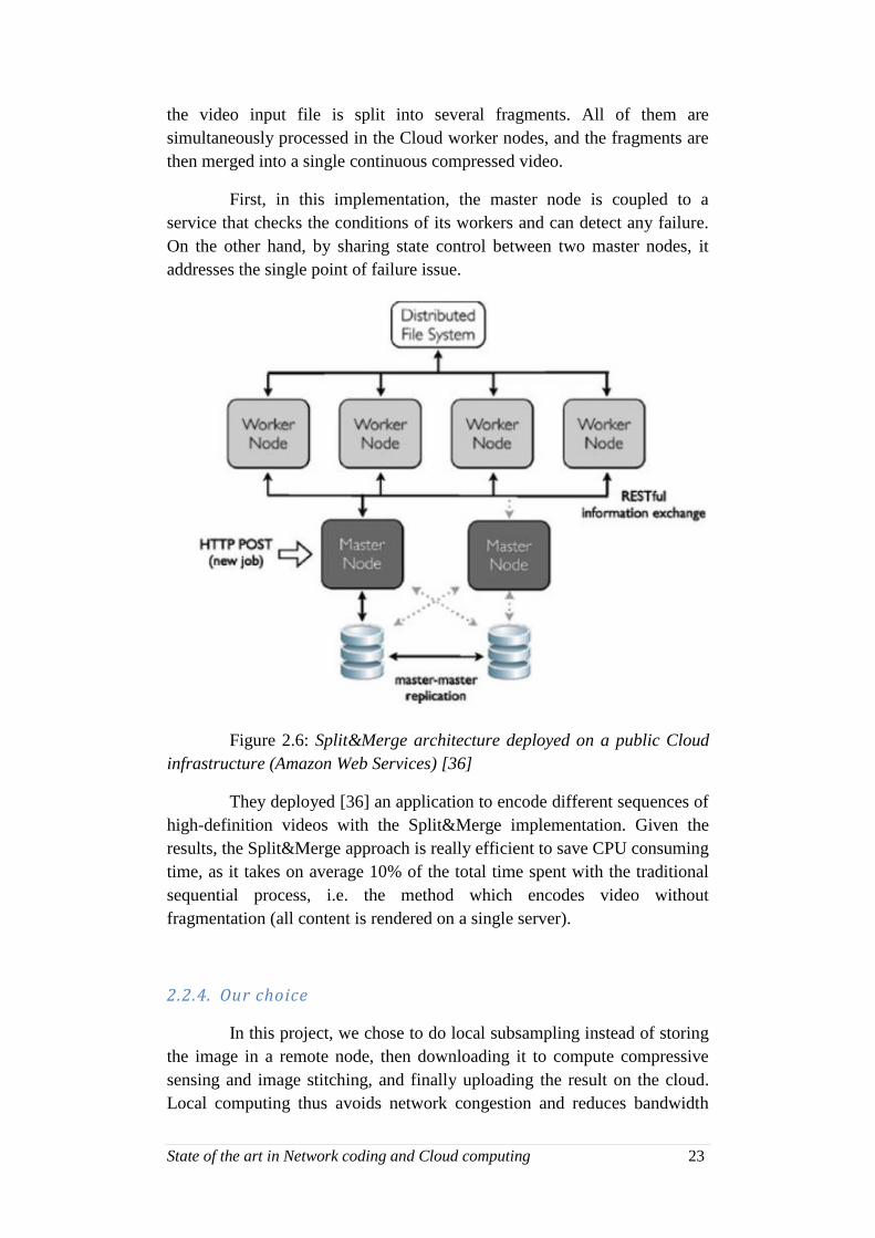
State of the art in Network coding and Cloud computing 23
the video input file is split into several fragments. All of them are
simultaneously processed in the Cloud worker nodes, and the fragments are
then merged into a single continuous compressed video.
First, in this implementation, the master node is coupled to a
service that checks the conditions of its workers and can detect any failure.
On the other hand, by sharing state control between two master nodes, it
addresses the single point of failure issue.
Figure 2.6: Split&Merge architecture deployed on a public Cloud
infrastructure (Amazon Web Services) [36]
They deployed [36] an application to encode different sequences of
high-definition videos with the Split&Merge implementation. Given the
results, the Split&Merge approach is really efficient to save CPU consuming
time, as it takes on average 10% of the total time spent with the traditional
sequential process, i.e. the method which encodes video without
fragmentation (all content is rendered on a single server).
2.2.4. Our choice
In this project, we chose to do local subsampling instead of storing
the image in a remote node, then downloading it to compute compressive
sensing and image stitching, and finally uploading the result on the cloud.
Local computing thus avoids network congestion and reduces bandwidth

State of the art in Network coding and Cloud computing 24
costs. Moreover, the performance of the cloud server would affect the
computation speed of the CS and stitching algorithms, so working locally
avoids the delivery time issue. However, we are aware that cloud computing
and cloud storage may become almost essential when video surveillance
systems reach a high number of cameras and thus a large amount of data to
be processed. In that case, securing data is very important for reasons of
privacy and confidentiality. We would need to implement network coding to
split and encrypt the video data prior to its storage in various devices and in
such a way that no single IoT device contains enough coded data to
compromise the privacy of the video streams if it is stolen.
State of the art in Compressive Sensing 25
Chapter 3
State of the art in Compressive Sensing
3.1. Compressive Sensing
3.1.1. Background
Signal sampling is an essential step in the digital signal
processing. The Nyquist sampling theory asserts that a band-limited signal
can be perfectly recovered from those samples if the signal is sampled at a
rate that is at least twice its bandwidth. This is the basic principle for almost
all the acquisition protocols in digital systems (e.g. electronics,
communication, biomedical imaging). However, this process does not
concern signals that are not naturally limited in the frequency domain, for
example magnetic signals. But the Nyquist theorem plays an implicit role
when such signals are processed to limit their frequency bandwidth before
sampling.
The Compressive Sensing theory was born a decade ago with the
work respectively of Candès, Romberg, Tao [6] [8] and Donoho [7] which
renew the Nyquist’s sampling theory regarding non band-limited signals.
The authors [6, 7, 8] propose sampling techniques that can reduce the
number of necessary measurements by determining this number more with
the amount of information in the signal than its frequency bandwidth.
This new approach uses the fact that a signal is sparse (i.e. the
signal is a combination of a limited number of non-zero coefficients) in a
known fixed orthonormal basis Ψ and can be recovered from a small set of
projections onto another orthonormal basis Փ, incoherent with the first one.
Roughly speaking, Փ and Ψ are incoherent if no element of one basis has a
sparse representation in terms of the other basis. Interestingly, random
projections are incoherent with any other fixed basis.
3.1.2. The sensing paradigm
Important questions can be raised when we consider under sampling
situations where the number m of measurements is much
smalleundersamplingr than the dimension n of the signal f:
Is it possible to recover accurately the signal from m<<n
measurements?
Is it possible to design m<<n sensing waveforms to get
almost all the information from f?
State of the art in Compressive Sensing 26
How can the signal f be approximated from this information?
Consider an m×n sensing matrix A with φ1*,…, φm
* as row-vectors (φ* being
the complex transpose of φ). The goal is to find f ϵ Rn from y = A. f ϵ Rm
,
which is often ill-posed when m˂n. Indeed, there is infinity of solution
signals 𝑓 for which A. 𝑓 = y. But one could find an escape by relying on
realistic models of objects f which naturally exist [8]. The Nyquist theory
states that if f(t) has a very low bandwidth, a small set of uniform samples is
enough to recover the signal. Candès and Wakin [8] show that signal
recovery is actually possible for a much wider class of signals.
3.1.3. Sparsity
Sparsity is a very important notion in signal processing. For
examples, cameras take colored-pictures (coded in three fundamental colors
R, G, B) of tens of million pixels. Each pixel being coded on 1 byte, it
would represent 30 Mb per picture. But files – generally coded in the JPEG
format – are much lighter than that. The key to efficient coding is the
sparsity notion. Consider signal composed of a vector in RN and an
orthonormal basis B={φ1,…, φN} in RN. The signal x ϵ RN
is sparse in the
basis B if x can be characterized by a small set of n << N coefficients
<x, φn> from its decomposition on B. Then,
𝑥(𝑡) = ∑ 𝒙i. φi(t)
𝑁
𝑖=1
(3-1)
The signal is sparse if one can discard the smallest coefficients
without losing too much information for a good recovery. The signal is
called S-parse when it has at most S non-zero coefficients. Actually, a huge
part of the data is redundant and a large fraction of the coefficients can be
thrown away. In [8], Candès and Wakin show that 97.5% of the coefficients
from a megapixel image can be discarded and the reconstructed image will
be very close to the original.
Last but not least, sparsity has a lot of potential on the acquisition
process as it determines how efficiently a signal can be acquired non-
adaptively.
State of the art in Compressive Sensing 27
3.1.4. Incoherent sampling
Consider a pair of orthonormal bases (Փ, Ψ) in Rn. The first base Փ
is used of the acquisition of the signal f and the second one Ψ to represent
f. The coherence between Փ where f is measured and Ψ where the signal is
sparse is [8]:
𝜇(Փ, Ψ) = √𝑛 . max1≤𝑘,𝑗≤𝑛
|⟨𝜑𝑘, 𝛹𝑗⟩|
(3-2)
This formula means that the coherence measures the highest
correlation between any of two columns of Փ and Ψ. From we linear
algebra, it follows that (Փ, Ψ) ϵ [1, √𝑛 ]. The more Փ and Ψ contain
correlated elements, the larger the coherence is.
Compressive sensing is interesting in duet of bases with low
coherence. If we consider the canonical basis Փ, φk=δ(t-k), and the Fourier
basis Ψ, Ψj=n-1/2
.𝑒𝑖2𝜋𝑗𝑡/𝑛. Since Փ is the sensing matrix, it corresponds to
the classical sampling scheme in time. The time-frequency pair gives
coherence 𝜇(Փ, Ψ) equals to 1 and so that is the maximal incoherence.
3.1.5. Sparse signals recovery
According to the Nyquist theorem, one would like to get n
coefficients from f, but according to the compressive sensing protocol, we
only acquire a part of them:
yk= ⟨𝑓, φ𝑘⟩, k ϵ M
where M ⊂ {1,…,n} is a subset of cardinality m<n
(3-3)
To recover the sparse representation of f, we have to solve an
optimization problem. Consider a vector x* for which y=Ψ.Փ.x*. To have
imperatively sparse signals after recovery, a natural approach is to impose
the l0 norm (defined as the non-zero coefficients) of the recovered signals to
be minimal:
min 𝑥 ϵ Rn‖�̂�‖l0 subject to yk=⟨φ𝑘, 𝛹�̂�⟩, ∀k ϵ M
(3-4)
‖�̂�‖ l0 (l0 norm of �̂�) represents the number of non-zero components
in the vector �̂�.
State of the art in Compressive Sensing 28
Davis, Mallat and Avallaneda [9] show that this constraint leads to
hard NP algorithms, and the exponential complexity makes them
unworkable for realistic values of n. However, the constraint on the l0 norm
can be lightened by imposing the l1 norm of recovered signals to be
minimal. Even though the l1 norm is a less optimal solution, it can at least be
computed by linear programming techniques.
Candès, Romberg, Tao [6] showed that a sparse signal can be
perfectly recovered from m measurements by solving the following
algorithm:
min 𝑥 ϵ Rn‖�̂�‖l1 subject to yk=⟨φ𝑘, 𝛹�̂�⟩, ∀k ϵ M
(3-5)
The only difference with the previous equation is that the support
size (number of non-zero components) is replaced by the sum of the
absolute values of those components. Then, the latest equation can be recast
as a linear program and solved by appropriate algorithms. Though the two
equations are fundamentally different, they give the same result in many
interesting situations, for some more measurements of yk in the second case.
3.1.6. The fundamental theorem in compressive sensing
Fix a signal f ϵ Rn, which is S-sparse in the basis Ψ. Select m
measurements uniformly at random in the basis Փ. Then if
𝑚 ≥ 𝐶. 𝜇2(Փ, Ψ). S. log (𝑛) (3-6)
for a certain positive constant C, the solution of (3-5) is exact with a very
high probability.
As explained by Candès and Wakin [8], three observations can be
made:
The role of the coherence is completely transparent; the smaller the
coherence, the fewer samples are needed, hence the importance to
choose two bases with low coherence.
No information is lost by measuring about any set of m coefficients
(m<n). If 𝜇(Փ, Ψ) equals or is close to 1, then we can take around
S.log(n) samples instead of n.
The signal f can be exactly recovered from a small set of data by
minimizing a convex problem, which does not require any
knowledge about the number of non-zero coefficients of x, nor about
their locations or their amplitudes, assumed all unknown a priori.
State of the art in Compressive Sensing 29
A good recovery algorithm can guarantee an exact reconstruction of
the signal if it is enough sparse. The theorem suggests a very useful sensing
protocol: sampling at random in an incoherent domain and use linear
programming for the recovery after the acquisition step. Thus, the signal
will be in a compressed form. To “decompress” it, we need a decoder,
which is guaranteed by the l1-minimization.
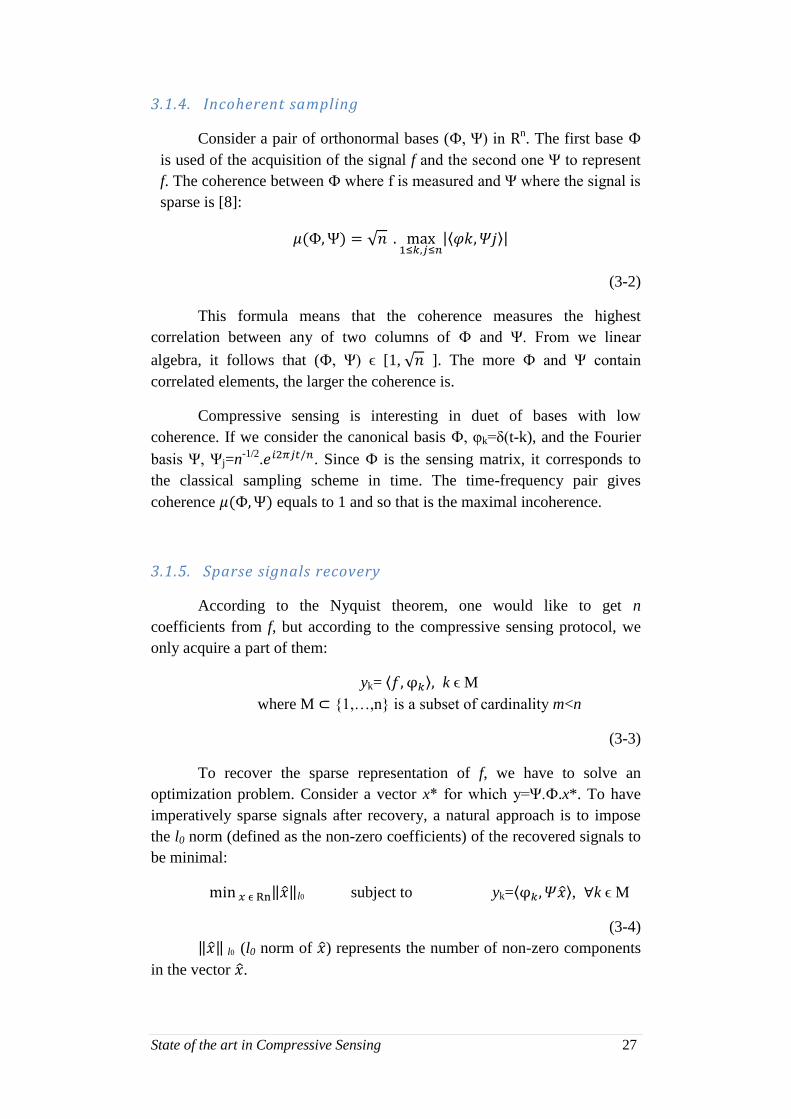
The figure below shows the different representations a signal can
have: a signal f, with a certain representation x with a sparsity S in the basis
Ψ, is sampled by a part of the basis Փ, incoherent with Ψ. From those
samples y – randomly chosen in Փ by following a uniform distribution – it
is possible to recover x by using convex optimization methods.
Figure 3.1: Several representations of a signal in different basis.
3.1.7. Interest of CS in surveillance video storage
Video surveillance cameras produce a huge amount of high
resolution data, which becomes a challenge to compute and store. But
transmitting all data to the cloud for further processing is, in many
applications, costly and unnecessary. For example, providing sensor data in
a farm or video surveillance would benefit from local storage and pre-
processing before upload to the cloud. CS exploits the fact that there is a
high redundancy in the image/video data.
The compressive sensing theory affirms that one can recover sparse
signals from a set of samples fewer than the number told by the
conventional methods. The CS techniques work as if it was possible to get
only the important part of the signal. By taking around S.log(n) random
samples (with S<<n) instead of n, we will still have enough information to
recover the signal.
In other words, CS measurement protocols mainly convert analog
data to digital only when the signal has already been compressed. Then,
after the acquisition and transmission steps, one only needs to decompress
the data.
State of the art in Compressive Sensing 30
3.2. Coupling of Network Coding and Compressive Sensing
As seen previously, a lot of research has been carried out in each of
those two fields over the past decades but the combination between network
coding and compressive sensing just started to be investigated a few years
ago, even though there are two powerful concepts for error control in
wireless sensor networks.
By combining and forwarding packets instead of simply sending
them to the destination, network coding has been proved very powerful to
improve network throughput and robustness, and thus performance and
reliability. However, this technique fails at decoding when the number of
received packets is less than the original one. On the other hand,
compressive sensing was found very efficient to process mutual correlation
of information and to drastically decrease the number of measurements, thus
highly reducing redundancy. Those two techniques are complementary and
their combination has been recently examined [21, 25-28]. Those works
tried to solve the limitation problem of NC.
On one hand, some works [25, 26] resulted in designing a
transformation matrix of NC which can adapt to the reconstruction
requirement of CS. In other words, the NC linear transformation process is
regarded as the acquisition process of CS measurement matrix. Among
them, Nguyen et al. [25] presented a practical scheme called Netcompress to
overcome the high link-failure rate in WSN. Their encoding framework uses
RLNC at adjacent source nodes and intermediate nodes, as well as the l1-
minimization CS reconstruction method. However, its designs of the packet
header and packet elimination mechanism are unclear. Nabaee et al. [26]
studied the combination of network coding and distributed source coding
from a CS perspective. In order to encode correlated sources without the
knowledge of the source correlation model, they proposed Quantized
Network coding, which incorporates real field NC and quantization to take
advantage of decoding using linear programming.
However, none of them reduced the number of redundant packets
transmitted, which does not solve the compression gain issue. It has been
nonetheless investigated in some other works. Luo et al. [27] presented a
joint source and network coding scheme, called Compressive Network
coding (CNC). They injected the concept of compressed sensing into
network coding to avoid the “all-or-nothing” problem of NC. It allows CNC
to achieve graceful degradation in data precisions to keep the energy
consumption at all nodes balanced. However they did not take into
consideration the noise in the sensor links. Yang et al. [28] elaborated a
compressed network coding based data storage scheme by exploiting the
correlation of sensor readings. This scheme achieves high energy efficiency

State of the art in Compressive Sensing 31
and guarantees good CS performance. It only focuses on network
performance without considering the errors or noise problem in transmission
process, which is known to have a huge impact on network performance.
Thus, a combination has been developed to overcome drawbacks of
NC theory by injecting CS concepts into it, called the ‘joint scheme’. It
exploits simultaneously the temporal and spatial correlations of the signal in
order to achieve the maximum gain. It has been confirmed by the reliability
analysis and numeric results that this joint scheme outperforms the
traditional network coding scheme both in robustness and in performance
terms.
Problem Statement 32
Chapter 4
Problem Statement
4.1. Importance of video surveillance
The security of humans, belongings and information has become a
major issue worldwide over the last decade. From fight against terrorism to
the strengthening of internal security through the rise of cybercrime, people
invest more and more to assure their protection. Information and
communication technologies bring new and sophisticated solutions for
physical and IT security. Among them, video surveillance is one of the
oldest and best-known security technologies.
Originally used by public services, it has been adopted by companies
to protect strategic assets and now in public or private places. Video
surveillance is mainly used for investigation purpose. Sometimes it requires
deploying tens or even hundreds of cameras in a large security area. And in
a world constantly becoming more digital, video surveillance is being
integrated with other security components into one single system.
Improvement of the software, the evolution from analog to digital video, the
increase in digital transmission speed and data encryption leads to a fully
integrated security system including video surveillance, alarm, access
control etc.
If analog video recording has gradually evolved to a digital
technology, the digital video recorder is evolving into a ‘virtual’ video
storage database located in a remote device. Video recording and storage is
then limited only by the size of the network computer memory capacity.
Video surveillance cameras produce a huge amount of high resolution data,
which becomes a challenge to compute and store. Thus, enterprise storage
systems dedicated to video surveillance need to have a larger throughput
capacity.
Due to their important size, surveillance data are usually not kept for
a long period of time – generally no longer than one month – which implies
that the captured activities cannot be browsed later, especially for forensic
purposes as evidence. In archival mode, video data storage and
manageability is the problem that toughens post-incident investigation. Due
to the temporary nature of video data, it is very difficult for a human to
analyse video data within a limited amount of time. Moreover, video images
need to have a good enough quality if we think in particular of face
recognition for example.
Problem Statement 33
4.2. Architecture of video surveillance systems
The first step in the video surveillance process is the acquisition.
There are diverse types of cameras to meet the surveillance needs. It goes
from analog to digital cameras, through fix, megapixel, panoramic or even
motorized cameras.
The video captured by the surveillance cameras must be transferred
to the recording, computing and viewing systems. It can be transmitted
through cables (e.g. coaxial cables, fibre, twisted pair copper wires) or
through the air (infrared signals, radio transmission). Wired video is the
most predominant in video surveillance systems. It offers a wider bandwidth
and a better reliability than wireless connections, for a lower price.
However, wireless video is inevitable for the surveillance of a wide area
where cables would be expensive to deploy or when the areas to be
monitored cannot be wired connected. Whether it is a wired or a wireless
transmission, the signal can be analog or digital even though it has
considerably evolved into digital videos. The IP protocol has played an
important role in the increasing use of LAN, WAN or Internet networks to
carry video data. IP cameras can directly connect to these networks, whereas
video streams from analog cameras need to be first digitized by an encoder
(also called video server) to transit over IP networks.
Digitized videos represent a huge amount of data to be computed and
stored. A bandwidth up to 165 MB/s can be required to send a video clip
and the data from a single camera over one day may fill 7 GB of disk space.
That is the reason why video surveillance data need to be compressed by
using codecs, i.e. algorithms that enable to reduce the quantity of data by
removing redundancy in each image or between the different footage
frames, as well as details undetectable by human eyesight. Depending on the
type of compression, more or less resources are used in the processor to
compute the codec. A compromise need to be found between the
compression rate and the processor resources. Currently, MJPEG and H.264
are the most widespread compression standards in video surveillance.
Video management systems process the video surveillance images,
such as managing the different video streams, viewing, recording, or doing
some analysis and research in the recorded footages. There are four broad
categories of video management systems:
Digital Video Recorder: It only takes flows from analog
cameras and digitizes them. The video can be viewed from a
remote computer. It has been mostly replaced by systems that
support IP video from end-to-end.
Hybrid Digital Video Recorder: It is similar to the DVR but it
can take flows from analog and IP cameras.
Problem Statement 34
Network Video Recorder: Designed for IP video surveillance
network architectures, it can only take video signals from IP
cameras or encoders.
IP video surveillance software: It is a purely software
solution to process video data in an IP network. In the case of
surveillance systems with few cameras, a Web browser can
be enough to manage the video. For bigger video surveillance
networks, softwares dedicated to video processing must be
used.
The archiving period varies according to the surveillance needs,
going from a couple of days to several years. The deployment of wide
camera networks and the high definition of the videos lead to a demand of
storage capacity more and more important, besides an increasing amount of
data to be stored. There are two categories of storage solutions:
Internal: Hard drives are incorporated in the digital video
recorders or in the servers. It is the most widespread solution,
offering up to four terabytes of space storage. Some IP
cameras have memory cards or USB disks that can store
several days of video recording. Internal archival solutions
are adapted for video surveillance systems of up to fifty
cameras.
Attached: Videos are archived on external devices such as
Network Attached Storage (NAS) or Storage Area Network
(SAN) that offer a storage space shared between several
customers in the network. On NAS devices, files are stored
on a single hard disk contrary to SAN storage that allows
storing fragments on different devices. Attached archival
solutions offer more advantage for large surveillance zones
with numerous cameras. Even though they are more
expensive than internal archival systems, these solutions are
much more accurate in terms of flexibility, expandability and
redundancy.
Research is still conducted to incorporate always more artificial
intelligence in the new video surveillance systems, in order to make them
more robust and efficient for security applications in a wide variety of
domains.
Problem Statement 35
4.3. Requirements and stakes in video analytics
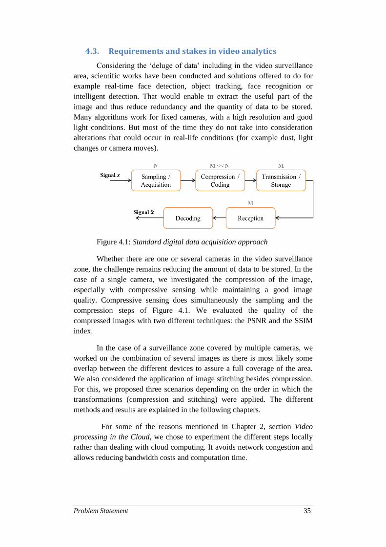
Considering the ‘deluge of data’ including in the video surveillance
area, scientific works have been conducted and solutions offered to do for
example real-time face detection, object tracking, face recognition or
intelligent detection. That would enable to extract the useful part of the
image and thus reduce redundancy and the quantity of data to be stored.
Many algorithms work for fixed cameras, with a high resolution and good
light conditions. But most of the time they do not take into consideration
alterations that could occur in real-life conditions (for example dust, light
changes or camera moves).
Figure 4.1: Standard digital data acquisition approach
Whether there are one or several cameras in the video surveillance
zone, the challenge remains reducing the amount of data to be stored. In the
case of a single camera, we investigated the compression of the image,
especially with compressive sensing while maintaining a good image
quality. Compressive sensing does simultaneously the sampling and the
compression steps of Figure 4.1. We evaluated the quality of the
compressed images with two different techniques: the PSNR and the SSIM
index.
In the case of a surveillance zone covered by multiple cameras, we
worked on the combination of several images as there is most likely some
overlap between the different devices to assure a full coverage of the area.
We also considered the application of image stitching besides compression.
For this, we proposed three scenarios depending on the order in which the
transformations (compression and stitching) were applied. The different
methods and results are explained in the following chapters.
For some of the reasons mentioned in Chapter 2, section Video
processing in the Cloud, we chose to experiment the different steps locally
rather than dealing with cloud computing. It avoids network congestion and
allows reducing bandwidth costs and computation time.
Single image processing: Compressive Sensing implementation 36
Chapter 5
Single image processing: Compressive Sensing
implementation
5.1. Simple Compressed Sensing examples
Implementation examples of compressed sensing applied to image
data are available on MathWorks website [10]. The Matlab code example
used follows the explanations given by Baraniuk [11].
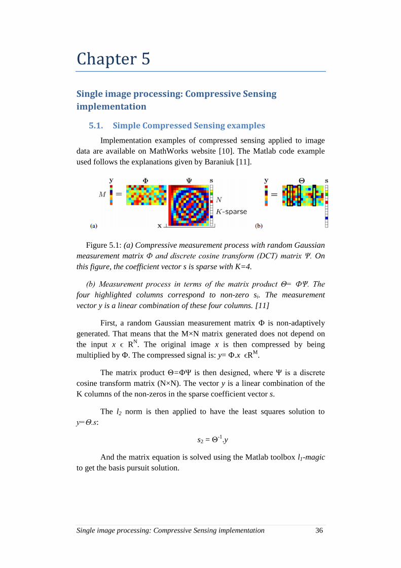
Figure 5.1: (a) Compressive measurement process with random Gaussian
measurement matrix Փ and discrete cosine transform (DCT) matrix Ψ. On
this figure, the coefficient vector s is sparse with K=4.
(b) Measurement process in terms of the matrix product Θ= ՓΨ. The
four highlighted columns correspond to non-zero si. The measurement
vector y is a linear combination of these four columns. [11]
First, a random Gaussian measurement matrix Փ is non-adaptively
generated. That means that the M×N matrix generated does not depend on
the input x ϵ RN. The original image x is then compressed by being
multiplied by Փ. The compressed signal is: y= Փ.x ϵRM
.
The matrix product Θ=ՓΨ is then designed, where Ψ is a discrete
cosine transform matrix (N×N). The vector y is a linear combination of the
K columns of the non-zeros in the sparse coefficient vector s.
The l2 norm is then applied to have the least squares solution to
y=Θ.s:
s2 = Θ-1
.y
And the matrix equation is solved using the Matlab toolbox l1-magic
to get the basis pursuit solution.
Single image processing: Compressive Sensing implementation 37
(a)
(b)
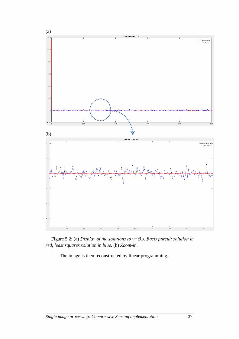
Figure 5.2: (a) Display of the solutions to y=Θ.s. Basis pursuit solution in
red, least squares solution in blue. (b) Zoom-in.
The image is then reconstructed by linear programming.
Single image processing: Compressive Sensing implementation 38
(a) (b)
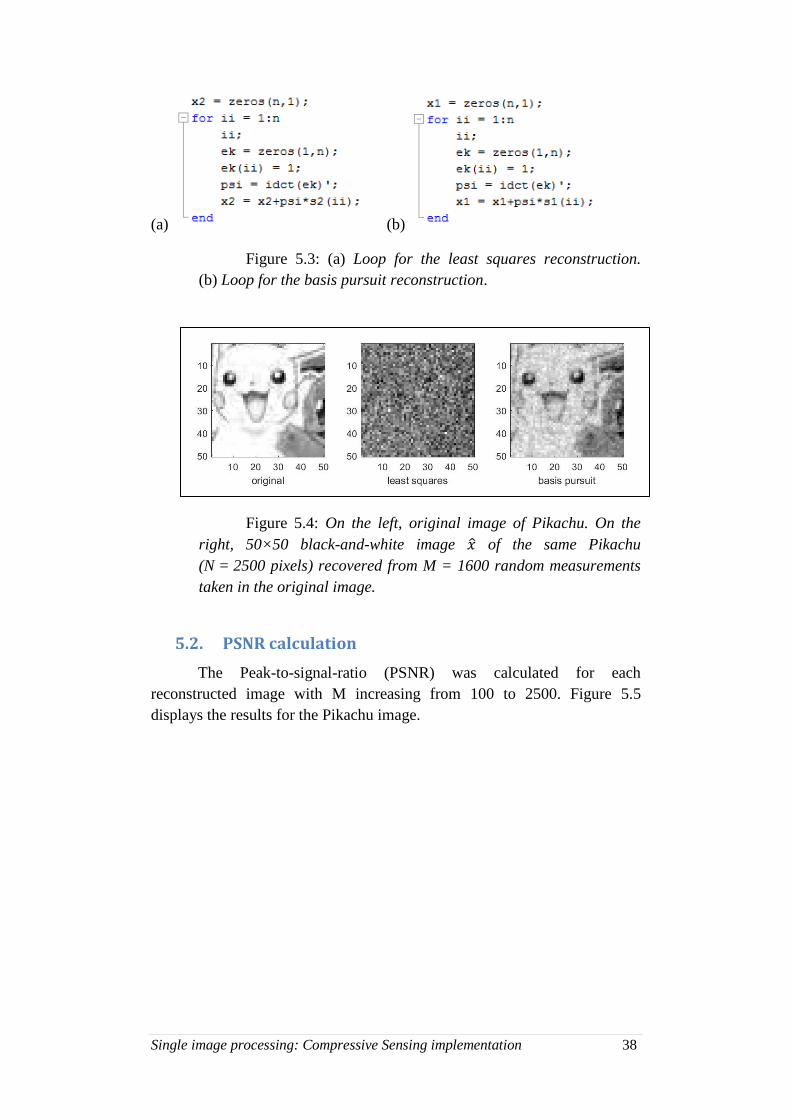
Figure 5.3: (a) Loop for the least squares reconstruction.
(b) Loop for the basis pursuit reconstruction.
Figure 5.4: On the left, original image of Pikachu. On the
right, 50×50 black-and-white image �̂� of the same Pikachu
(N = 2500 pixels) recovered from M = 1600 random measurements
taken in the original image.
5.2. PSNR calculation
The Peak-to-signal-ratio (PSNR) was calculated for each
reconstructed image with M increasing from 100 to 2500. Figure 5.5
displays the results for the Pikachu image.
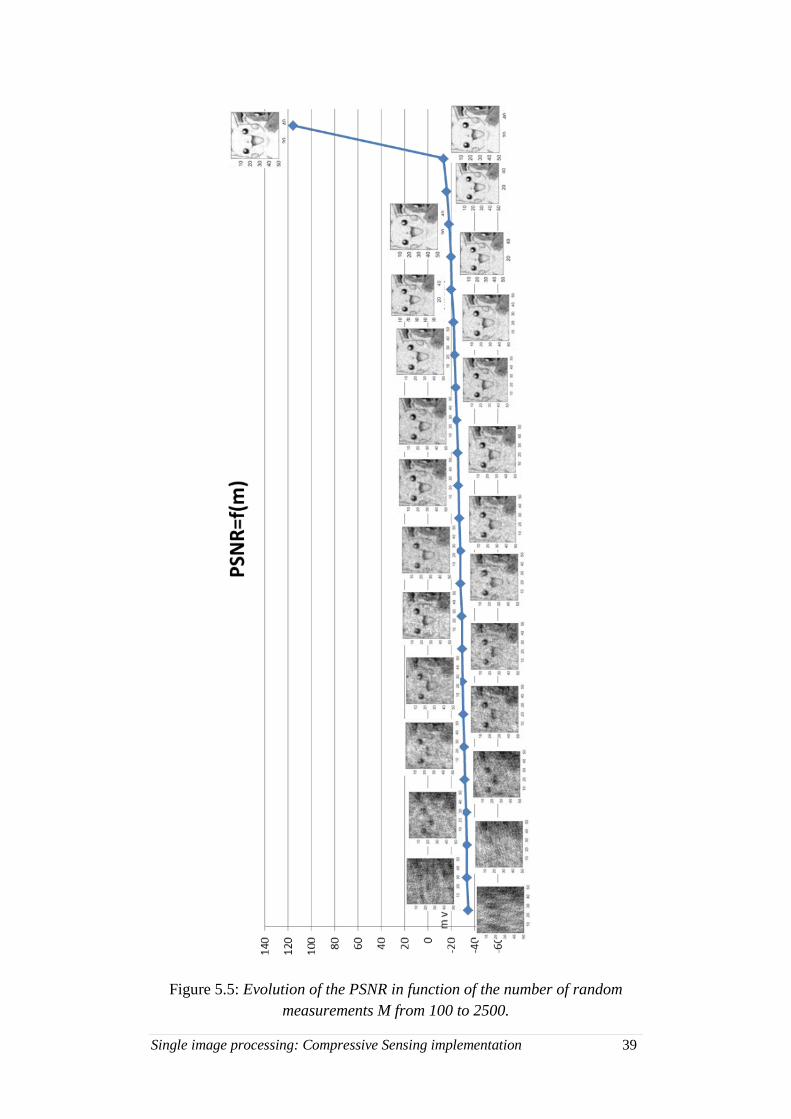
Single image processing: Compressive Sensing implementation 39
Figure 5.5: Evolution of the PSNR in function of the number of random
measurements M from 100 to 2500.
Single image processing: Compressive Sensing implementation 40
The PSNR is the ratio between the maximum possible power of a
signal and the power of corrupting noise that affects the fidelity of its
representation. Thus, it can be used to measure the quality of reconstruction
for image compression. In this case, the signal is the original data and the
noise is the error introduced by compression. It is generally expressed in the
logarithmic decibel scale, with this formula:
PSNR = 20.log10 ( 𝑀𝐴𝑋𝑖
√𝑀𝑆𝐸)
or PSNR= 20.log10(𝑀𝐴𝑋𝑖) – 10.log10(𝑀𝑆𝐸)
(5-1)
MAXi is the maximum possible pixel value of the image, i.e. 255
(= 2^8 -1) when the pixels are represented with 8 bits per sample. MSE –
standing for Mean-Squared Error – measures the difference between two
images, the original image 𝑥(𝑎, 𝑏) and the “degraded” image �̂�(𝑎, 𝑏). The
MSE represents the average of the squares of the "errors" between the
original image and the compressed one. The error is the amount by which
the values of the original image differ from the degraded image. The MSE
is:
MSE = 1
𝑀.𝑁∑ ∑ [𝑁
𝑗=1𝑀𝑖=1 �̂�(𝑖, 𝑗) − 𝑥(𝑖, 𝑗)]²
(5-2)
M is the number of rows of pixels in the images and i is the index of
that row; N is the number of columns of pixels in the images and j is the
index of that column.
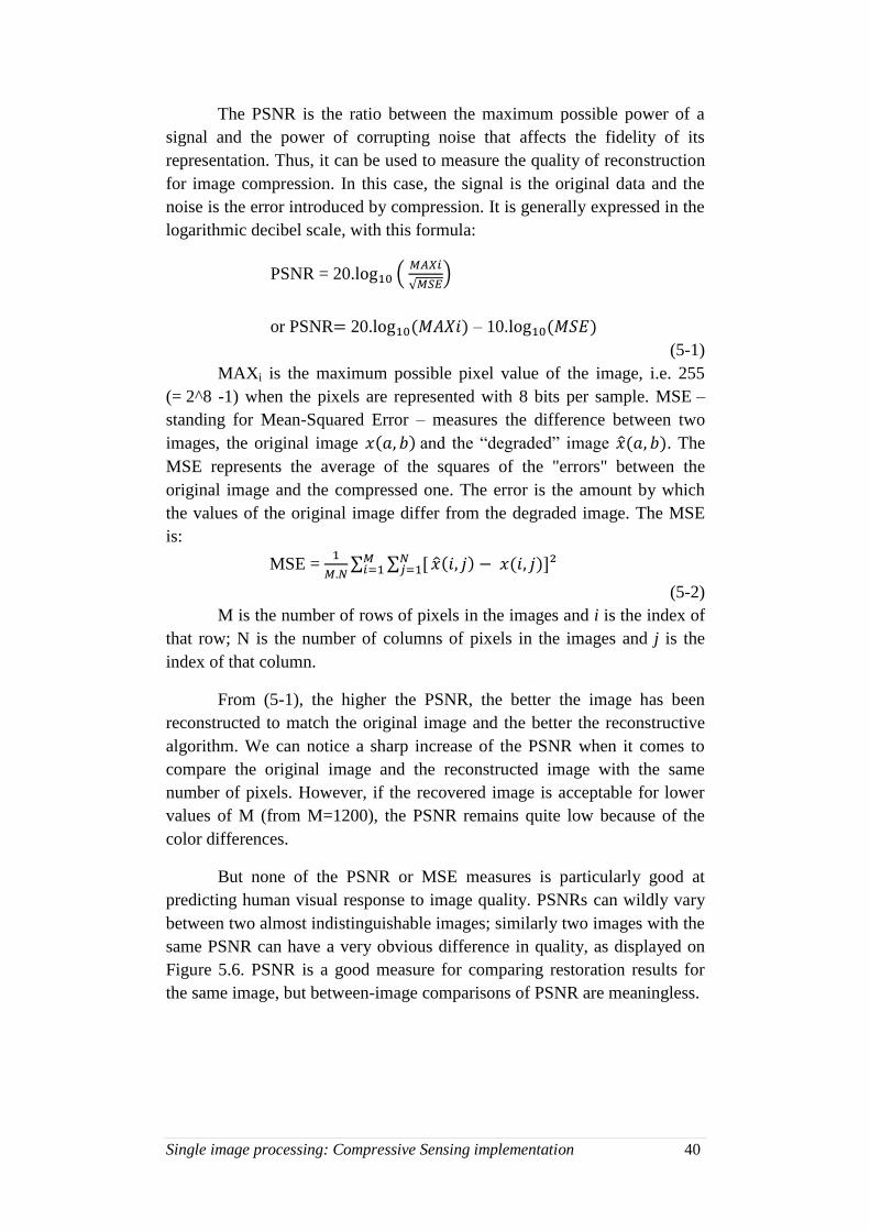
From (5-1), the higher the PSNR, the better the image has been
reconstructed to match the original image and the better the reconstructive
algorithm. We can notice a sharp increase of the PSNR when it comes to
compare the original image and the reconstructed image with the same
number of pixels. However, if the recovered image is acceptable for lower
values of M (from M=1200), the PSNR remains quite low because of the
color differences.
But none of the PSNR or MSE measures is particularly good at
predicting human visual response to image quality. PSNRs can wildly vary
between two almost indistinguishable images; similarly two images with the
same PSNR can have a very obvious difference in quality, as displayed on
Figure 5.6. PSNR is a good measure for comparing restoration results for
the same image, but between-image comparisons of PSNR are meaningless.
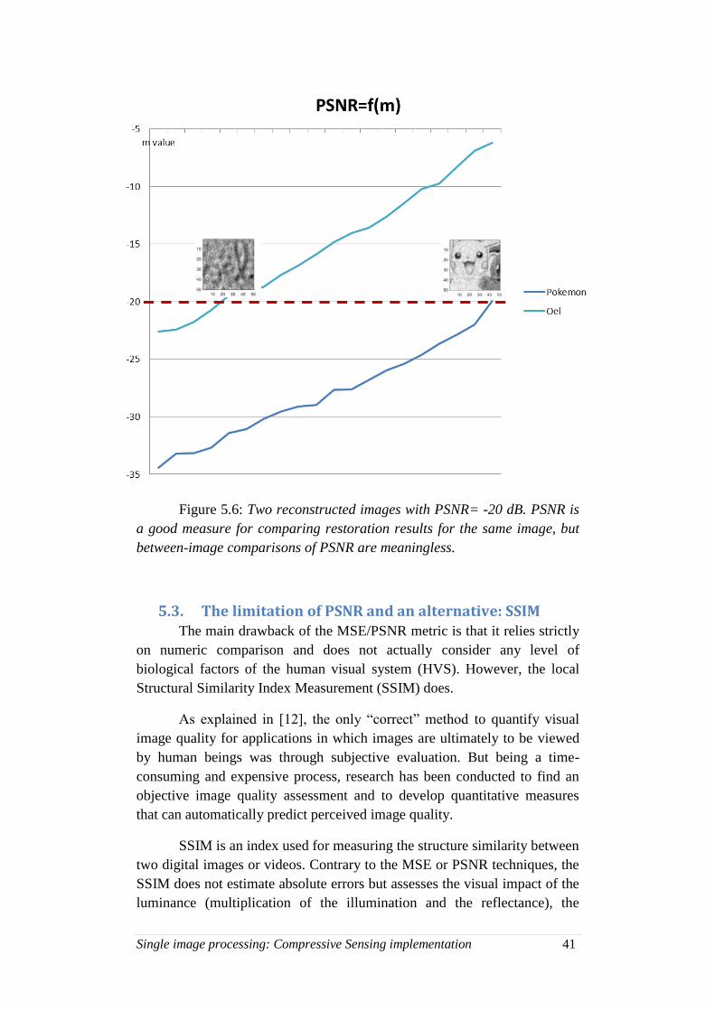
Single image processing: Compressive Sensing implementation 41
Figure 5.6: Two reconstructed images with PSNR= -20 dB. PSNR is
a good measure for comparing restoration results for the same image, but
between-image comparisons of PSNR are meaningless.
5.3. The limitation of PSNR and an alternative: SSIM The main drawback of the MSE/PSNR metric is that it relies strictly
on numeric comparison and does not actually consider any level of
biological factors of the human visual system (HVS). However, the local
Structural Similarity Index Measurement (SSIM) does.
As explained in [12], the only “correct” method to quantify visual
image quality for applications in which images are ultimately to be viewed
by human beings was through subjective evaluation. But being a time-
consuming and expensive process, research has been conducted to find an
objective image quality assessment and to develop quantitative measures
that can automatically predict perceived image quality.
SSIM is an index used for measuring the structure similarity between
two digital images or videos. Contrary to the MSE or PSNR techniques, the
SSIM does not estimate absolute errors but assesses the visual impact of the
luminance (multiplication of the illumination and the reflectance), the
Single image processing: Compressive Sensing implementation 42
contrast and the structure of the image. It is a modification of the MSE so
that errors are quantified according to their visibility. This error-sensitivity
approach is based on several assumptions and generalizations, summarized
by Wang et al [12]:
The Quality Definition Problem: The error visibility does not
necessarily lead to quality loss, as some distortions may be
noticeable but not so damaging.
The Suprathreshold Problem: Threshold values at which a
stimulus is just barely visible are measured and then used to
define visual errors sensitivity measures. Yet, it is indicated
by only a few psychophysical studies that these threshold
values can be generalized to characterize perceptual
distortions significantly larger than the threshold levels.
The Natural Image Complexity Problem: The patterns used
during most psychophysical experiments are simpler than
real world images so the model may not predict the visual
quality of complex-structured natural images.
The Decorrelation Problem: There is a strong dependency
between intra- and inter-channel wavelet coefficients of
natural images. But it has been shown that optimal design of
transformation and masking models can reduce both
statistical and perceptual dependencies.
The Cognitive Interaction Problem: Cognitive understanding
and eye movements influence the perception of image
quality. Most image quality metrics do not consider those
effects, as they are very difficult to quantify and not well
understood.
The structural information is those attributes that represent the
structure of the objects in a visual scene, independently of the average
luminance and contrast. To explore the structural information, it has to be
separated from the influence of the illumination. As structural information is
the idea that pixels are highly interdependent especially when they are
spatially close, it is useful for image quality assessment to apply the SSIM
index locally rather than globally.
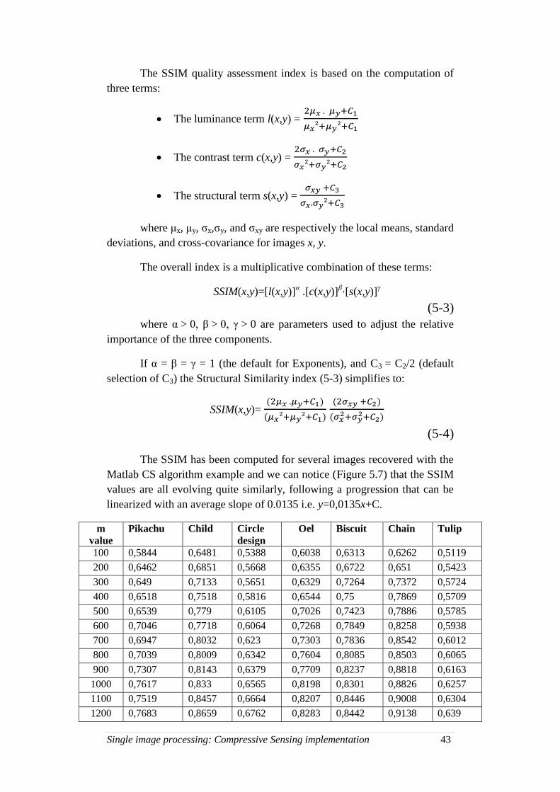
Single image processing: Compressive Sensing implementation 43
The SSIM quality assessment index is based on the computation of
three terms:
The luminance term l(x,y) = 2𝜇𝑥 . 𝜇𝑦+𝐶1
𝜇𝑥²+𝜇𝑦²+𝐶1
The contrast term c(x,y) = 2𝜎𝑥 . 𝜎𝑦+𝐶2
𝜎𝑥²+𝜎𝑦²+𝐶2
The structural term s(x,y) = 𝜎𝑥𝑦 +𝐶3
𝜎𝑥.𝜎𝑦²+𝐶3
where μx, μy, σx,σy, and σxy are respectively the local means, standard
deviations, and cross-covariance for images x, y.
The overall index is a multiplicative combination of these terms:
SSIM(x,y)=[l(x,y)]α .[c(x,y)]
β⋅[s(x,y)]γ
(5-3)
where α > 0, β > 0, γ > 0 are parameters used to adjust the relative
importance of the three components.
If α = β = γ = 1 (the default for Exponents), and C3 = C2/2 (default
selection of C3) the Structural Similarity index (5-3) simplifies to:
SSIM(x,y)= (2𝜇𝑥 .𝜇𝑦+𝐶1)
(𝜇𝑥²+𝜇𝑦²+𝐶1)
(2𝜎𝑥𝑦 +𝐶2)
(𝜎𝑥2+𝜎𝑦
2+𝐶2)
(5-4)
The SSIM has been computed for several images recovered with the
Matlab CS algorithm example and we can notice (Figure 5.7) that the SSIM
values are all evolving quite similarly, following a progression that can be
linearized with an average slope of 0.0135 i.e. y=0,0135x+C.
m
value
Pikachu Child Circle
design
Oel Biscuit Chain Tulip
100 0,5844 0,6481 0,5388 0,6038 0,6313 0,6262 0,5119
200 0,6462 0,6851 0,5668 0,6355 0,6722 0,651 0,5423
300 0,649 0,7133 0,5651 0,6329 0,7264 0,7372 0,5724
400 0,6518 0,7518 0,5816 0,6544 0,75 0,7869 0,5709
500 0,6539 0,779 0,6105 0,7026 0,7423 0,7886 0,5785
600 0,7046 0,7718 0,6064 0,7268 0,7849 0,8258 0,5938
700 0,6947 0,8032 0,623 0,7303 0,7836 0,8542 0,6012
800 0,7039 0,8009 0,6342 0,7604 0,8085 0,8503 0,6065
900 0,7307 0,8143 0,6379 0,7709 0,8237 0,8818 0,6163
1000 0,7617 0,833 0,6565 0,8198 0,8301 0,8826 0,6257
1100 0,7519 0,8457 0,6664 0,8207 0,8446 0,9008 0,6304
1200 0,7683 0,8659 0,6762 0,8283 0,8442 0,9138 0,639
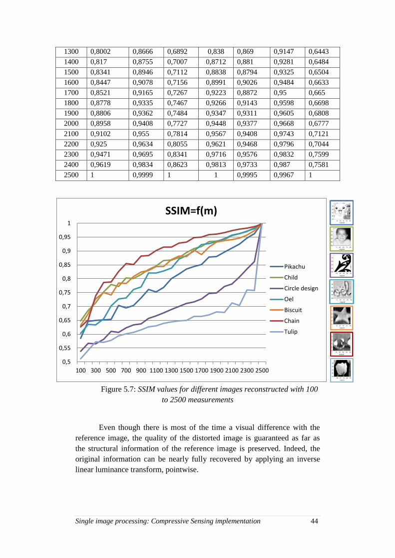
Single image processing: Compressive Sensing implementation 44
1300 0,8002 0,8666 0,6892 0,838 0,869 0,9147 0,6443
1400 0,817 0,8755 0,7007 0,8712 0,881 0,9281 0,6484
1500 0,8341 0,8946 0,7112 0,8838 0,8794 0,9325 0,6504
1600 0,8447 0,9078 0,7156 0,8991 0,9026 0,9484 0,6633
1700 0,8521 0,9165 0,7267 0,9223 0,8872 0,95 0,665
1800 0,8778 0,9335 0,7467 0,9266 0,9143 0,9598 0,6698
1900 0,8806 0,9362 0,7484 0,9347 0,9311 0,9605 0,6808
2000 0,8958 0,9408 0,7727 0,9448 0,9377 0,9668 0,6777
2100 0,9102 0,955 0,7814 0,9567 0,9408 0,9743 0,7121
2200 0,925 0,9634 0,8055 0,9621 0,9468 0,9796 0,7044
2300 0,9471 0,9695 0,8341 0,9716 0,9576 0,9832 0,7599
2400 0,9619 0,9834 0,8623 0,9813 0,9733 0,987 0,7581
2500 1 0,9999 1 1 0,9995 0,9967 1
Figure 5.7: SSIM values for different images reconstructed with 100
to 2500 measurements
Even though there is most of the time a visual difference with the
reference image, the quality of the distorted image is guaranteed as far as
the structural information of the reference image is preserved. Indeed, the
original information can be nearly fully recovered by applying an inverse
linear luminance transform, pointwise.
0,5
0,55
0,6
0,65
0,7
0,75
0,8
0,85
0,9
0,95
1
100 300 500 700 900 1100 1300 1500 1700 1900 2100 2300 2500
SSIM=f(m)
Pikachu
Child
Circle design
Oel
Biscuit
Chain
Tulip
Single image processing: Compressive Sensing implementation 45
5.4. Edge detection In an image, an edge can be defined as a set of contiguous pixels
where a sudden change of intensity – gray or colour – occurs. As
compressive sensing takes random samples, we thought that edge detection
could be applied after the CS step to evaluate the reconstruction. It would
determine if CS recovers edges accurately and a sampling threshold could
then be set up regarding the edge detection results.
Edge detection aims at identifying points in an image where there
are brightness discontinuities. The points where brightness changes sharply
generally form a set of curved line segments named edges. Edges are often
associated with the boundaries of objects. Edge detection is used to identify
the edges in a digital image. In Matlab, the edges can be found with the edge
function which attempts to detect places in the image where the intensity
changes rapidly. Several edge detection methods exist, but most of them can
be classified into two categories:
First-order derivative methods: These methods search
extrema in first-order derivative expressions, usually the local maxima of
the gradient of the image.
Second-order derivative methods: The second methods
search for zero crossings in second-order derivative expressions, usually the
zero-crossings of the Laplacian or of a non-linear differential expression.
“Edge provides a number of derivative estimators, each of which
implements one of the definitions above. For some of these estimators, you
can specify whether the operation should be sensitive to horizontal edges,
vertical edges, or both. Edge returns a binary image containing 1's where
edges are found and 0's elsewhere.” [14]
Edge detection algorithms usually give a set of connected curves
that correspond to the boundaries of objects as well as curves that reveal
discontinuities in surface orientation. Applying edge detection to an image
enables to reduce significantly the amount of data to be processed. It filters
out information that may be regarded as less relevant and only keeps the
important structural properties of an image. It is perfectly illustrated on
Figure 5.8: the SSIM values are higher from the very first samples with an
edge detection filter than the SSIM values displayed on Figure 5.7 without
doing any edge detection.
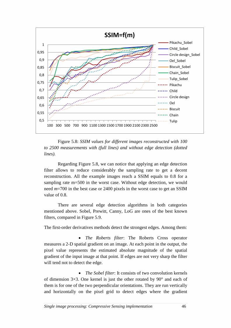
Single image processing: Compressive Sensing implementation 46
Figure 5.8: SSIM values for different images reconstructed with 100
to 2500 measurements with (full lines) and without edge detection (dotted
lines).
Regarding Figure 5.8, we can notice that applying an edge detection
filter allows to reduce considerably the sampling rate to get a decent
reconstruction. All the example images reach a SSIM equals to 0.8 for a
sampling rate m=500 in the worst case. Without edge detection, we would
need m=700 in the best case or 2400 pixels in the worst case to get an SSIM
value of 0.8.
There are several edge detection algorithms in both categories
mentioned above. Sobel, Prewitt, Canny, LoG are ones of the best known
filters, compared in Figure 5.9.
The first-order derivatives methods detect the strongest edges. Among them:
The Roberts filter: The Roberts Cross operator
measures a 2-D spatial gradient on an image. At each point in the output, the
pixel value represents the estimated absolute magnitude of the spatial
gradient of the input image at that point. If edges are not very sharp the filter
will tend not to detect the edge.
The Sobel filter: It consists of two convolution kernels
of dimension 3×3. One kernel is just the other rotated by 90° and each of
them is for one of the two perpendicular orientations. They are run vertically
and horizontally on the pixel grid to detect edges where the gradient
0,5
0,55
0,6
0,65
0,7
0,75
0,8
0,85
0,9
0,95
1
100 300 500 700 900 1100 1300 1500 1700 1900 2100 2300 2500
SSIM=f(m) Pikachu_Sobel
Child_Sobel
Circle design_Sobel
Oel_Sobel
Biscuit_Sobel
Chain_Sobel
Tulip_Sobel
Pikachu
Child
Circle design
Oel
Biscuit
Chain
Tulip

Single image processing: Compressive Sensing implementation 47
magnitude is high. The kernels can then be combined together to find the
absolute magnitude of the gradient at each point and the orientation of that
gradient. This makes the Sobel edge detector more sensitive to diagonal
edge than horizontal and vertical edges. It is the default edge detection filter
in Matlab (used in Figure 5.8).
The Prewitt filter: It is a discrete differentiation
operator which is similar to the Sobel operator, by computing the gradient
for the image intensity function. Compared to Sobel, the Prewitt masks are
simpler to implement but are very sensitive to noise.
The Canny filter: It is often referred as the optimal
edge detector, as it uses a multi-stage algorithm to detect edges in an image.
The Canny algorithm finds edges by looking for local maxima of the
gradient of an image, using the derivative of a Gaussian filter. This method
uses two thresholds to detect strong and weak edges, including weak edges
in the output if they are connected to strong edges. By using two thresholds,
the Canny method is less likely than the other methods to be fooled by
noise, and more likely to detect true weak edges. An edge detection operator
that uses a multi-stage algorithm to detect a wide range of edges in images.
Sobel and Prewitt methods provide good edge maps very
effectively and are cheap to compute. By default, Matlab edge detection
algorithms use Sobel filter.
The zero-crossings of the second-order derivatives are good to
localize the edges. Those methods are more sophisticated towards
automatized edge detection, but still very noise-sensitive. As differentiation
amplifies noise, smoothing is suggested prior to applying the Laplacians.
Typical examples of second-order derivative edge detection methods are:
The Difference of Gaussian (DoG): It is a feature
enhancement algorithm involving the subtraction of one blurred version of
an original image from another, less blurred version of the original.
The Laplacian of Gaussian (LoG): The Laplacian is a
2-D isotropic measure of the second spatial derivative of an image. The LoG
operator is called so as the Laplacian is generally applied to an image that
has first been smoothed with a Gaussian smoothing filter to reduce its
sensitivity to noise. It takes a single grayscale image as input and produces
another grayscale image as output.
Image derivatives are commonly used in motion estimation and
object tracking in video. However, the optimal edge detection method
depends on the type of edges to be detected in an image (step edges, ramp
edges, lines or roof edges) and also on the application domain.
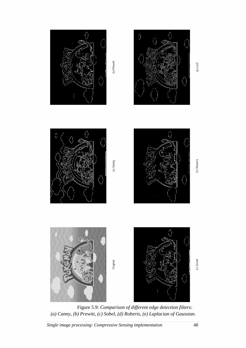
Single image processing: Compressive Sensing implementation 48
Figure 5.9: Comparison of different edge detection filters:
(a) Canny, (b) Prewitt, (c) Sobel, (d) Roberts, (e) Laplacian of Gaussian.
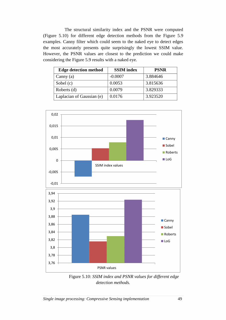
Single image processing: Compressive Sensing implementation 49
The structural similarity index and the PSNR were computed
(Figure 5.10) for different edge detection methods from the Figure 5.9
examples. Canny filter which could seem to the naked eye to detect edges
the most accurately presents quite surprisingly the lowest SSIM value.
However, the PSNR values are closest to the prediction we could make
considering the Figure 5.9 results with a naked eye.
Edge detection method SSIM index PSNR
Canny (a) -0.0007 3.884646
Sobel (c) 0.0053 3.815636
Roberts (d) 0.0079 3.829333
Laplacian of Gaussian (e) 0.0176 3.923520
Figure 5.10: SSIM index and PSNR values for different edge
detection methods.
-0,01
-0,005
0
0,005
0,01
0,015
0,02
SSIM index values
Canny
Sobel
Roberts
LoG
3,76
3,78
3,8
3,82
3,84
3,86
3,88
3,9
3,92
3,94
PSNR values
Canny
Sobel
Roberts
LoG
Single image processing: Compressive Sensing implementation 50
5.5. Conclusion In this chapter, we saw that signal sparsity can be exploited.
Taking random samples from an image by applying compressive sensing
gives good result for a number of pixels far smaller than the original image
resolution. That confirms that CS must be useful to deal with the ‘deluge of
data’ occurring in particular in the video surveillance world with the spread
of high resolution cameras.
Furthermore, as compressive sensing takes random samples, we
evaluated the accuracy of edge reconstruction in the CS algorithm. For that,
we applied edge detection filters on the recovered images. The results
clearly showed that edge detection would enable to considerably lower the
sample rate – compared to CS without edge detection – to reach a given
SSIM threshold.
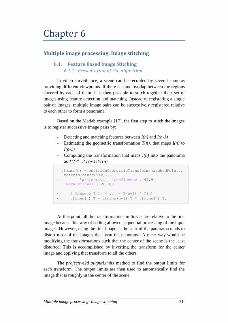
Multiple image processing: Image stitching 51
Chapter 6
Multiple image processing: Image stitching
6.1. Feature Based Image Stitching
6.1.1. Presentation of the algorithm
In video surveillance, a scene can be recorded by several cameras
providing different viewpoints. If there is some overlap between the regions
covered by each of them, it is then possible to stitch together their set of
images using feature detection and matching. Instead of registering a single
pair of images, multiple image pairs can be successively registered relative
to each other to form a panorama.
Based on the Matlab example [17], the first step to stitch the images
is to register successive image pairs by:
- Detecting and matching features between I(n) and I(n-1)
- Estimating the geometric transformation T(n), that maps I(n) to
I(n-1)
- Computing the transformation that maps I(n) into the panorama
as T(1)*…*T(n-1)*T(n).
- tforms(n) = estimateGeometricTransform(matchedPoints, matchedPointsPrev,...
- 'projective', 'Confidence', 99.9, 'MaxNumTrials', 2000);
-
- % Compute T(1) * ... * T(n-1) * T(n)
- tforms(n).T = tforms(n-1).T * tforms(n).T;
At this point, all the transformations in tforms are relative to the first
image because this way of coding allowed sequential processing of the input
images. However, using the first image as the start of the panorama tends to
distort most of the images that form the panorama. A nicer way would be
modifying the transformations such that the center of the scene is the least
distorted. This is accomplished by inverting the transform for the center
image and applying that transform to all the others.
The projective2d outputLimits method to find the output limits for
each transform. The output limits are then used to automatically find the
image that is roughly in the center of the scene.
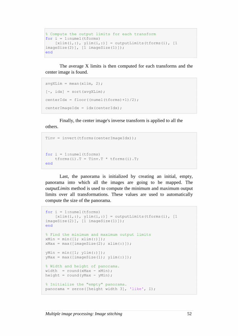
Multiple image processing: Image stitching 52
% Compute the output limits for each transform
for i = 1:numel(tforms)
[xlim(i,:), ylim(i,:)] = outputLimits(tforms(i), [1
imageSize(2)], [1 imageSize(1)]);
end
The average X limits is then computed for each transforms and the
center image is found.
avgXLim = mean(xlim, 2);
[~, idx] = sort(avgXLim);
centerIdx = floor((numel(tforms)+1)/2);
centerImageIdx = idx(centerIdx);
Finally, the center image's inverse transform is applied to all the
others.
Tinv = invert(tforms(centerImageIdx));
for i = 1:numel(tforms)
tforms(i).T = Tinv.T * tforms(i).T;
end
Last, the panorama is initialized by creating an initial, empty,
panorama into which all the images are going to be mapped. The
outputLimits method is used to compute the minimum and maximum output
limits over all transformations. These values are used to automatically
compute the size of the panorama.
for i = 1:numel(tforms)
[xlim(i,:), ylim(i,:)] = outputLimits(tforms(i), [1
imageSize(2)], [1 imageSize(1)]);
end
% Find the minimum and maximum output limits
xMin = min([1; xlim(:)]);
xMax = max([imageSize(2); xlim(:)]);
yMin = min([1; ylim(:)]);
yMax = max([imageSize(1); ylim(:)]);
% Width and height of panorama.
width = round(xMax - xMin);
height = round(yMax - yMin);
% Initialize the "empty" panorama.
panorama = zeros([height width 3], 'like', I);
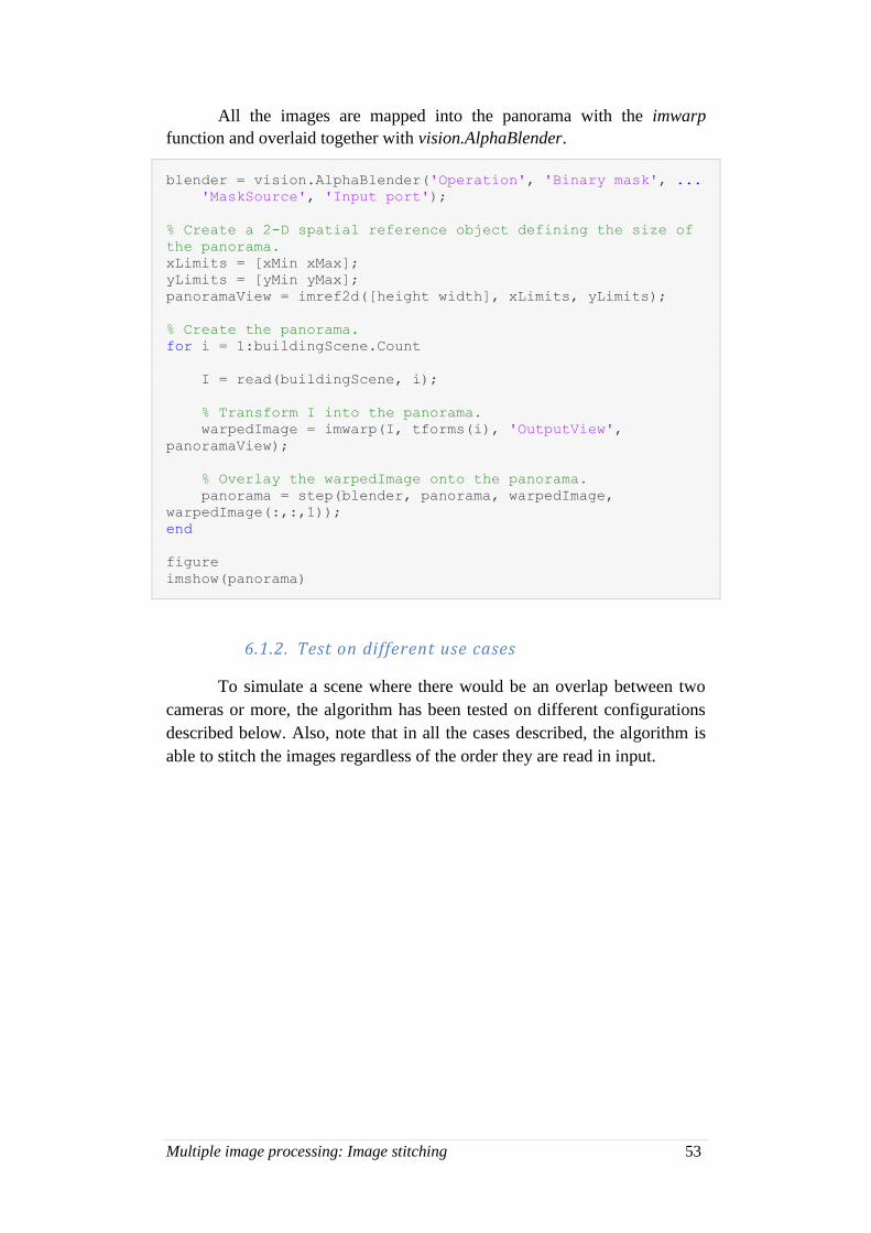
Multiple image processing: Image stitching 53
All the images are mapped into the panorama with the imwarp
function and overlaid together with vision.AlphaBlender.
blender = vision.AlphaBlender('Operation', 'Binary mask', ...
'MaskSource', 'Input port');
% Create a 2-D spatial reference object defining the size of
the panorama.
xLimits = [xMin xMax];
yLimits = [yMin yMax];
panoramaView = imref2d([height width], xLimits, yLimits);
% Create the panorama.
for i = 1:buildingScene.Count
I = read(buildingScene, i);
% Transform I into the panorama.
warpedImage = imwarp(I, tforms(i), 'OutputView',
panoramaView);
% Overlay the warpedImage onto the panorama.
panorama = step(blender, panorama, warpedImage,
warpedImage(:,:,1));
end
figure
imshow(panorama)
6.1.2. Test on different use cases
To simulate a scene where there would be an overlap between two
cameras or more, the algorithm has been tested on different configurations
described below. Also, note that in all the cases described, the algorithm is
able to stitch the images regardless of the order they are read in input.
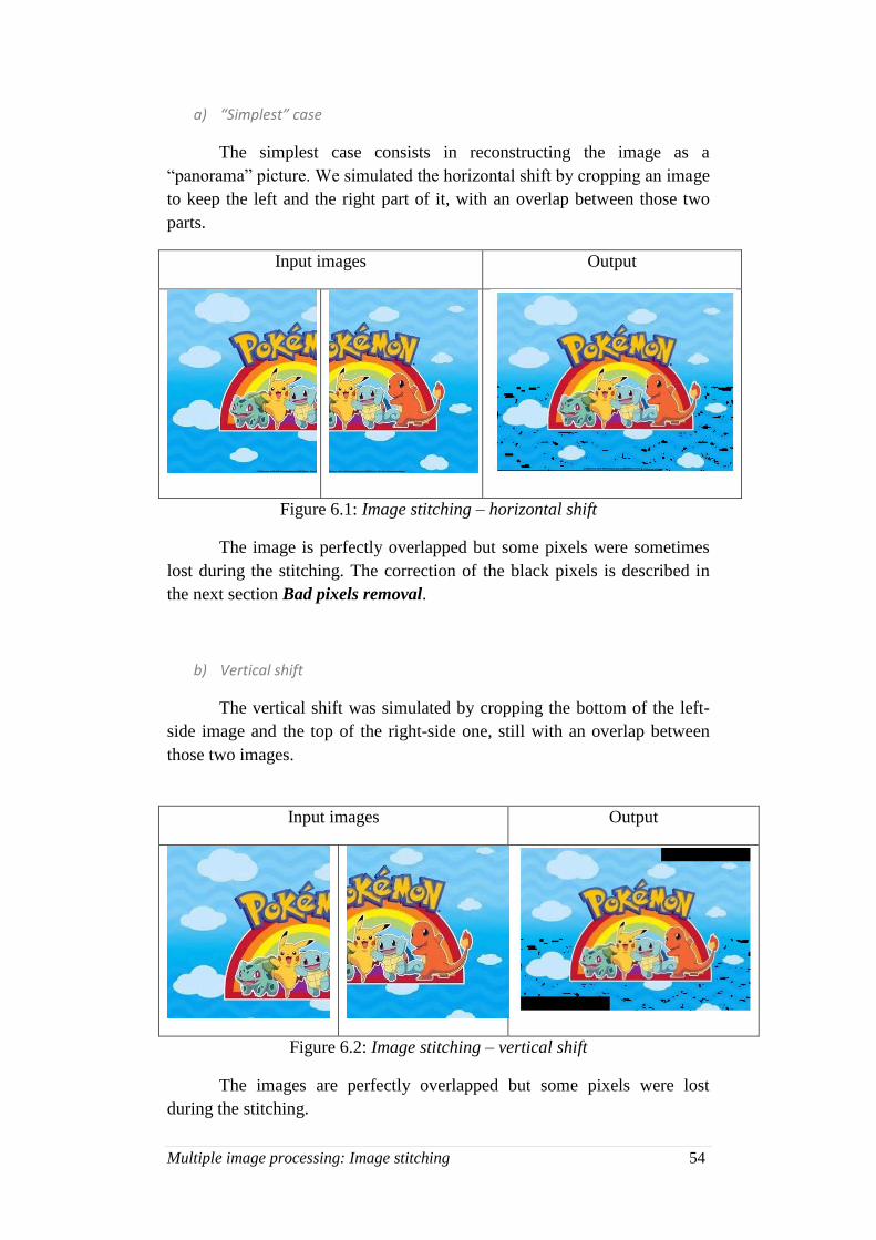
Multiple image processing: Image stitching 54
a) “Simplest” case
The simplest case consists in reconstructing the image as a
“panorama” picture. We simulated the horizontal shift by cropping an image
to keep the left and the right part of it, with an overlap between those two
parts.
Input images Output
Figure 6.1: Image stitching – horizontal shift
The image is perfectly overlapped but some pixels were sometimes
lost during the stitching. The correction of the black pixels is described in
the next section Bad pixels removal.
b) Vertical shift
The vertical shift was simulated by cropping the bottom of the left-
side image and the top of the right-side one, still with an overlap between
those two images.
Input images Output
Figure 6.2: Image stitching – vertical shift
The images are perfectly overlapped but some pixels were lost
during the stitching.

Multiple image processing: Image stitching 55
c) Tilt
The left part of the image was slightly tilted.
Input images Output
Figure 6.3: Image stitching – tilt
The images are perfectly stitched but some pixels were lost during
the stitching.
d) More than two input images
The algorithm was tested with a number of inputs superior to two.
The figure displays the stitching result of three different parts of the
Pokemon picture – overlapping two by two – and including one rotated 90
degrees. The images are perfectly gathered but some pixels were still lost
during the stitching.
Input images Output
Figure 6.4: Image stitching – 3 input images
e) “Real-life” case
A more “videosurveillance-oriented” case was simulated with street
view pictures taken from a same point and scanning a landscape.
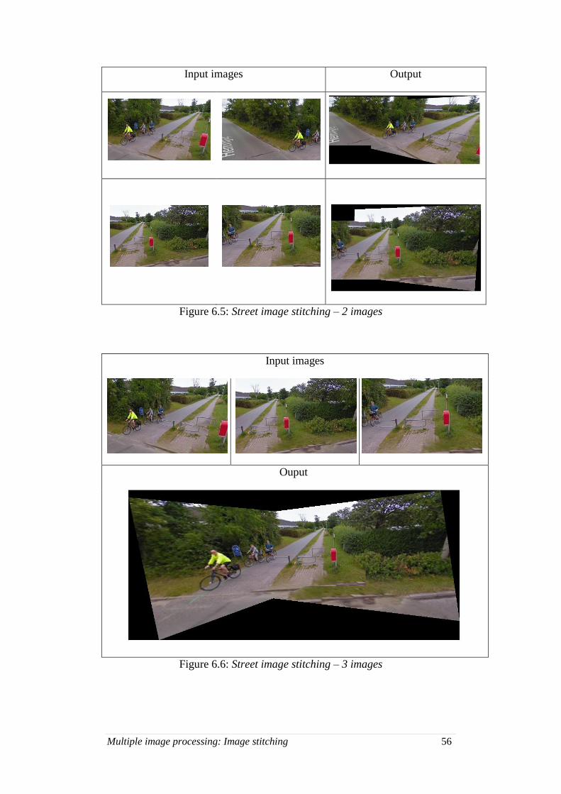
Multiple image processing: Image stitching 56
Input images Output
Figure 6.5: Street image stitching – 2 images
Input images
Ouput
Figure 6.6: Street image stitching – 3 images
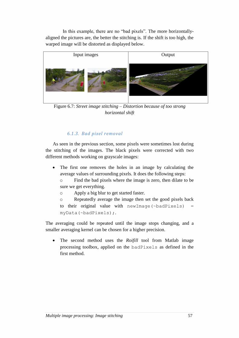
Multiple image processing: Image stitching 57
In this example, there are no “bad pixels”. The more horizontally-
aligned the pictures are, the better the stitching is. If the shift is too high, the
warped image will be distorted as displayed below.
Input images Output
Figure 6.7: Street image stitching – Distortion because of too strong
horizontal shift
6.1.3. Bad pixel removal
As seen in the previous section, some pixels were sometimes lost during
the stitching of the images. The black pixels were corrected with two
different methods working on grayscale images:
The first one removes the holes in an image by calculating the
average values of surrounding pixels. It does the following steps:
o Find the bad pixels where the image is zero, then dilate to be
sure we get everything.
o Apply a big blur to get started faster.
o Repeatedly average the image then set the good pixels back
to their original value with newImage(~badPixels) =
myData(~badPixels);.
The averaging could be repeated until the image stops changing, and a
smaller averaging kernel can be chosen for a higher precision.
The second method uses the Roifill tool from Matlab image
processing toolbox, applied on the badPixels as defined in the
first method.
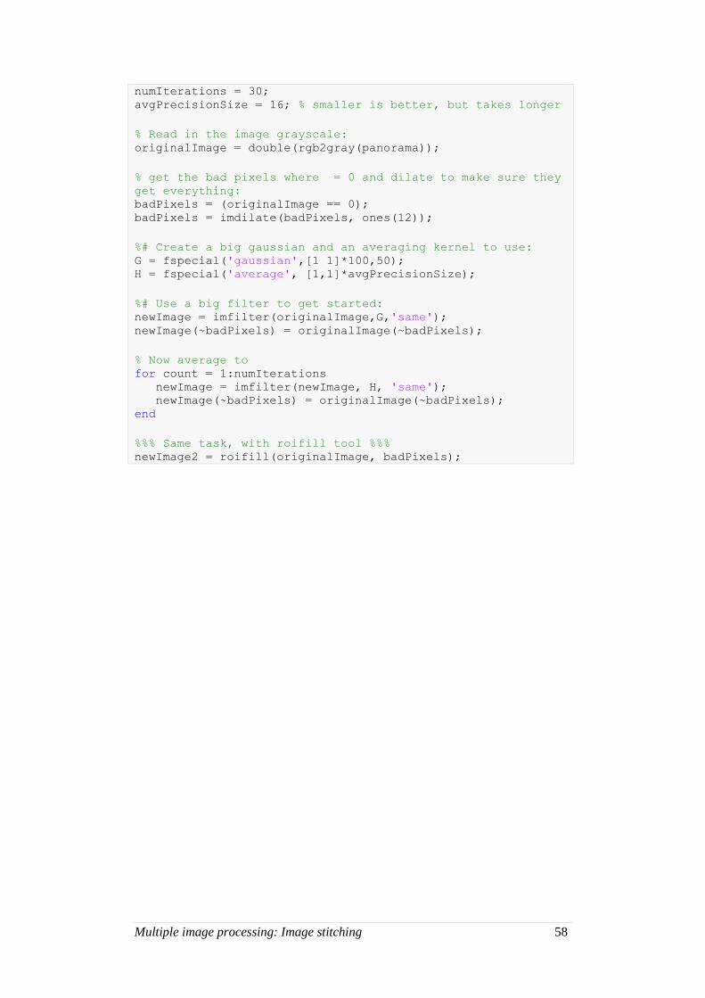
Multiple image processing: Image stitching 58
numIterations = 30; avgPrecisionSize = 16; % smaller is better, but takes longer
% Read in the image grayscale: originalImage = double(rgb2gray(panorama));
% get the bad pixels where = 0 and dilate to make sure they
get everything: badPixels = (originalImage == 0); badPixels = imdilate(badPixels, ones(12));
%# Create a big gaussian and an averaging kernel to use: G = fspecial('gaussian',[1 1]*100,50); H = fspecial('average', [1,1]*avgPrecisionSize);
%# Use a big filter to get started: newImage = imfilter(originalImage,G,'same'); newImage(~badPixels) = originalImage(~badPixels);
% Now average to for count = 1:numIterations newImage = imfilter(newImage, H, 'same'); newImage(~badPixels) = originalImage(~badPixels); end
%%% Same task, with roifill tool %%% newImage2 = roifill(originalImage, badPixels);
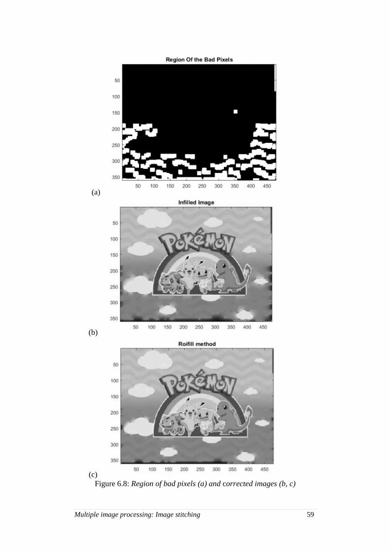
Multiple image processing: Image stitching 59
(a)
(b)
(c)
Figure 6.8: Region of bad pixels (a) and corrected images (b, c)
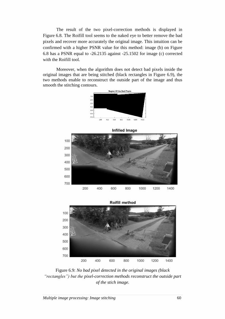
Multiple image processing: Image stitching 60
The result of the two pixel-correction methods is displayed in
Figure 6.8. The Roifill tool seems to the naked eye to better remove the bad
pixels and recover more accurately the original image. This intuition can be
confirmed with a higher PSNR value for this method: image (b) on Figure
6.8 has a PSNR equal to -26.2135 against -25.1502 for image (c) corrected
with the Roifill tool.
Moreover, when the algorithm does not detect bad pixels inside the
original images that are being stitched (black rectangles in Figure 6.9), the
two methods enable to reconstruct the outside part of the image and thus
smooth the stitching contours.
Figure 6.9: No bad pixel detected in the original images (black
“rectangles”) but the pixel-correction methods reconstruct the outside part
of the stich image.
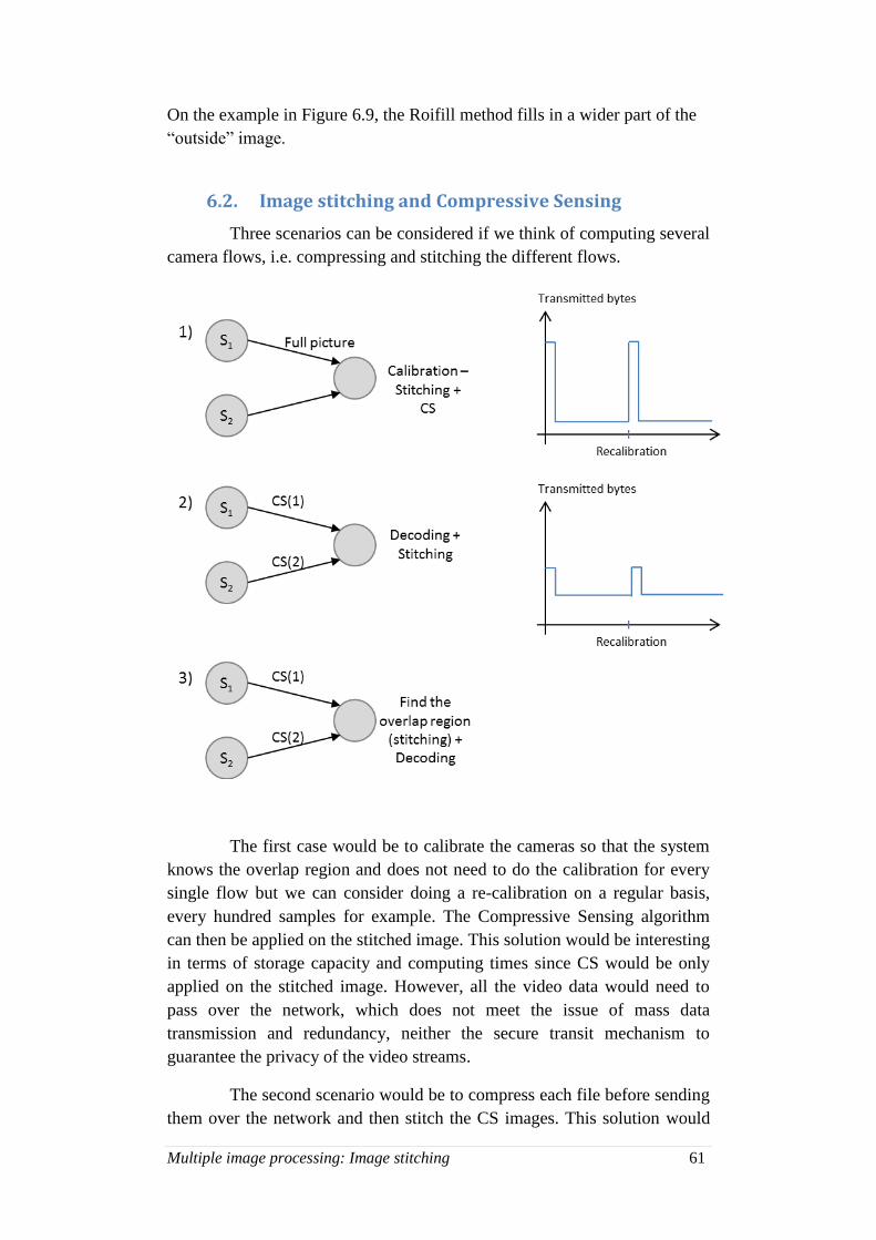
Multiple image processing: Image stitching 61
On the example in Figure 6.9, the Roifill method fills in a wider part of the
“outside” image.
6.2. Image stitching and Compressive Sensing
Three scenarios can be considered if we think of computing several
camera flows, i.e. compressing and stitching the different flows.
The first case would be to calibrate the cameras so that the system
knows the overlap region and does not need to do the calibration for every
single flow but we can consider doing a re-calibration on a regular basis,
every hundred samples for example. The Compressive Sensing algorithm
can then be applied on the stitched image. This solution would be interesting
in terms of storage capacity and computing times since CS would be only
applied on the stitched image. However, all the video data would need to
pass over the network, which does not meet the issue of mass data
transmission and redundancy, neither the secure transit mechanism to
guarantee the privacy of the video streams.
The second scenario would be to compress each file before sending
them over the network and then stitch the CS images. This solution would
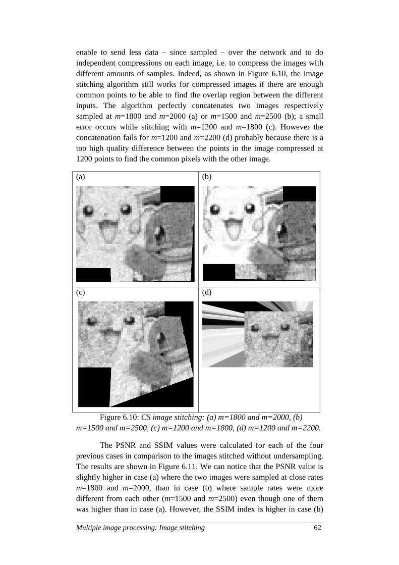
Multiple image processing: Image stitching 62
enable to send less data – since sampled – over the network and to do
independent compressions on each image, i.e. to compress the images with
different amounts of samples. Indeed, as shown in Figure 6.10, the image
stitching algorithm still works for compressed images if there are enough
common points to be able to find the overlap region between the different
inputs. The algorithm perfectly concatenates two images respectively
sampled at m=1800 and m=2000 (a) or m=1500 and m=2500 (b); a small
error occurs while stitching with m=1200 and m=1800 (c). However the
concatenation fails for m=1200 and m=2200 (d) probably because there is a
too high quality difference between the points in the image compressed at
1200 points to find the common pixels with the other image.
(a)
(b)
(c)
(d)
Figure 6.10: CS image stitching: (a) m=1800 and m=2000, (b)
m=1500 and m=2500, (c) m=1200 and m=1800, (d) m=1200 and m=2200.
The PSNR and SSIM values were calculated for each of the four
previous cases in comparison to the images stitched without undersampling.
The results are shown in Figure 6.11. We can notice that the PSNR value is
slightly higher in case (a) where the two images were sampled at close rates
m=1800 and m=2000, than in case (b) where sample rates were more
different from each other (m=1500 and m=2500) even though one of them
was higher than in case (a). However, the SSIM index is higher in case (b)
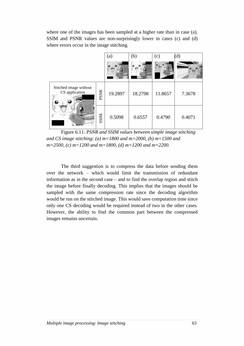
Multiple image processing: Image stitching 63
where one of the images has been sampled at a higher rate than in case (a).
SSIM and PSNR values are non-surprisingly lower in cases (c) and (d)
where errors occur in the image stitching.
(a)
(b)
(c)
(d)
Stitched image without
CS application
PS
NR
19.2897 18.2798 11.8657 7.3678
SS
IM
0.5098 0.6557 0.4790 0.4071
Figure 6.11: PSNR and SSIM values between simple image stitching
and CS image stitching: (a) m=1800 and m=2000, (b) m=1500 and
m=2500, (c) m=1200 and m=1800, (d) m=1200 and m=2200.
The third suggestion is to compress the data before sending them
over the network – which would limit the transmission of redundant
information as in the second case – and to find the overlap region and stitch
the image before finally decoding. This implies that the images should be
sampled with the same compression rate since the decoding algorithm
would be run on the stitched image. This would save computation time since
only one CS decoding would be required instead of two in the other cases.
However, the ability to find the common part between the compressed
images remains uncertain.
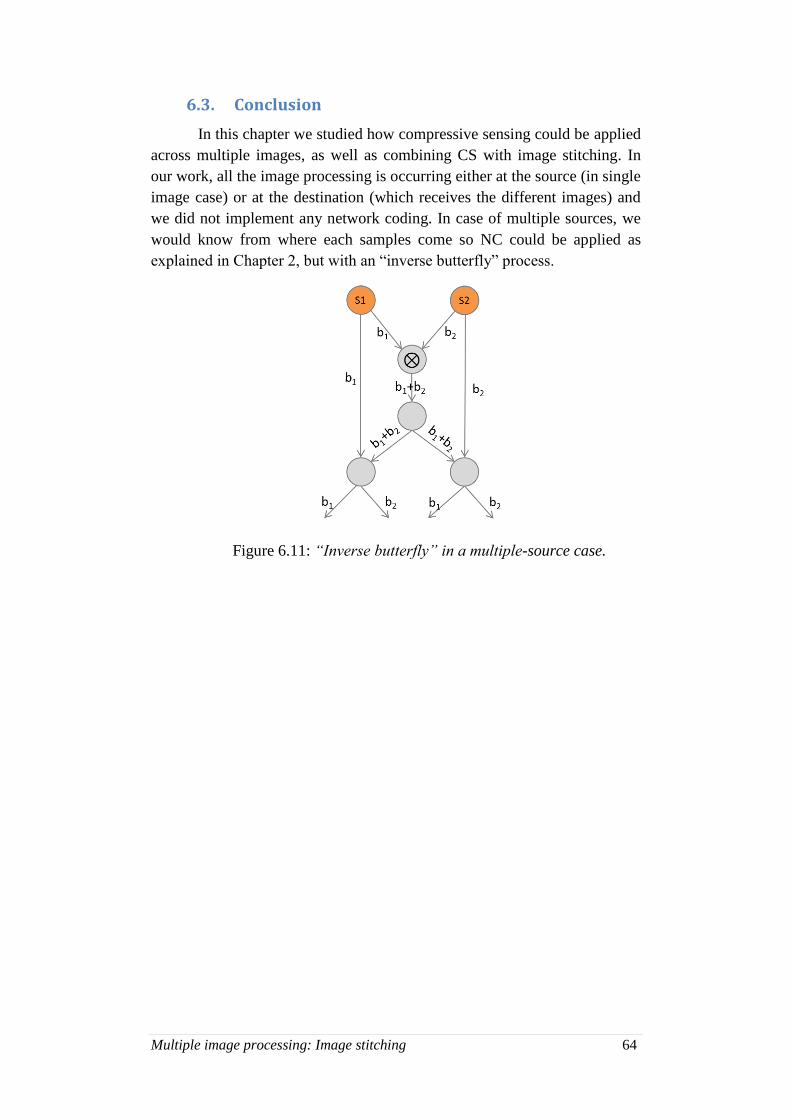
Multiple image processing: Image stitching 64
6.3. Conclusion
In this chapter we studied how compressive sensing could be applied
across multiple images, as well as combining CS with image stitching. In
our work, all the image processing is occurring either at the source (in single
image case) or at the destination (which receives the different images) and
we did not implement any network coding. In case of multiple sources, we
would know from where each samples come so NC could be applied as
explained in Chapter 2, but with an “inverse butterfly” process.
Figure 6.11: “Inverse butterfly” in a multiple-source case.

Conclusion and future work 65
Chapter 7
Conclusion and future work
The goal of this report was to evaluate the plausibility of applying
compressive sensing on video surveillance data, as part of an efficient
protocol that could automatically translate analog data into already
compressed digital form to be later computed for reconstruction. Through
this report we also considered the use of network coding as a way to manage
the distributed storage of video information.
In this project we studied an algorithm of image compressive
sensing, as video is a sequence of images. We evaluated the quality of the
results with two different mathematical tools. The first one, the PSNR
measured the quality of the reconstructed image by measuring the noise
introduced by compression. For video surveillance purpose, we thought we
could focus on the reconstruction accuracy of the image structure. Therefore
we measured the structural similarity with the SSIM index, which takes into
account the visual impact of the luminance, the contrast and the structure of
the image. We also found interesting to compare the results by applying
edge detection filters on the reconstructed images. It proved that edge
detection on CS images would enable to considerably reduce the number of
samples if we want to reach a given threshold.
On the other hand, we thought about a multi-camera video
surveillance scene and found an algorithm able to find the overlap region
between images and to stitch them together. We also considered the
different scenarios possible to combine image stitching and compressive
sensing, where the images could have been under sampled at different rates.
Several problems need to be addressed in a practical
implementation. For example, if cameras record a scene from different
angles, the perspective should be considered and adjusted during the
stitching. The possibility of implementing the combination between image
stitching and compressive sensing should be evaluated in the case where we
would like to find the overlap region between compressed images and stitch
them together before finally decoding. Moreover, we applied edge detection
filters after compressing the image in order to set up a threshold. We could
consider to adopt the opposite approach, which would apply edge detection
before the CS algorithm to filter out the ‘non relevant’ information and
compress even less data by working on the structure of the images.

Conclusion and future work 66
The security in these distributed storage systems is another topic
that must be deepened. Network coding must be implemented to split and
encrypt the data prior to its storage in various devices and in such a way that
no single IoT device contains enough coded data to compromise the privacy
of the video streams if it is stolen. Moreover, cloud computing and cloud
storage are developing massively to face the huge amount of information
IoT generates. Protection of this data is even more important as it is
processed and stored in third-party data centers. Cloud security is an issue
that should not be taken for granted and must be further investigated.
Sources 67
Sources
[1] John Gantz, David Reinsel. The Digital Universe in 2020. In Big Data,
Bigger Digital Shadows, and Biggest Growth in the Far East,
December 2012.
[2] IHS Technology. Video Surveillance & Storage: Opportunities at the
Intersection of IT and Physical Security, September 2014.
[3] Josh Woodhouse. Big, big, big data: higher and higher resolution video
surveillance, January 2016. URL:
https://technology.ihs.com/571026/big-big-big-data-higher-and-higher-
resolution-video-surveillance.
[4] Network coding definition. Techopedia. URL:
https://www.techopedia.com/definition/14833/network-coding.
[5] Hulya Seferoglu, Athina Markopoulou. Opportunistic Network coding
for Video Streaming over Wireless. In Packet Video 2007, pages 191-
200. IEEE, 2007. doi: 10.1109/PACKET.2007.4397041.
[6] Emmanuel Candès, Justin Romberg, Terence Tao. Stable Signal
Recovery from Incomplete and Inaccurate Measurements. In Comm.
Pure Appl. Math., Volume 59, pages 1207–1223, 2006.
doi:10.1002/cpa.20124.
[7] David L. Donoho. Compressed Sensing, Manuscript, September 2004.
[8] Emmanuel Candès and Michael Wakin. An Introduction to Compressive
Sampling. In IEEE Signal Processing Magazine, Volume 25, Issue 2,
pages 21–30, March 2008.
[9] G. Davis, S. Mallat, M. Avellaneda. Adaptive greedy approximations. In
Constructive Approximation, Volume 13, Issue 1, pages 57-98, March
1997.
[10] Stuart Gibson. Simple compressed sensing example, May 2013. URL:
http://www.mathworks.com/matlabcentral/fileexchange/41792-simple-
compressed-sensing-example .
[11] R. Baraniuk, Compressive Sensing, Lecture Notes in IEEE Signal
Processing Magazine, Volume 24, July 2007.
[12] Zhou Wang, Alan C. Bovik, Hamid R. Sheikh, and Eero P. Simoncelli.
Image Quality Assessment: From Error Visibility to Structural
Similarity. In IEEE Transactions on Image Processing, Volume 13,
Issue 4, pages 600–612, April 2004.
Sources 68
[13] Juan Cabrera. Content Delivery and Storage in Wireless Networks
Using Network coding. Aalborg University Master Thesis, June 2015.
[14] MathWorks Documentation, Image Processing Toolbox (SSIM, Edge
Detection). URL: http://fr.mathworks.com/help/images/.
[15] Yunhe Li, Qinyu Zhang, Shaohua Wu and Ruofei Zhou. Efficient Data
Gathering with Network coding Coupled Compressed Sensing for
Wireless Sensor Networks. In Information Technology Journal,
Volume 12, Issue 9, pages 1737-1745.
Doi: 10.3923/itj.2013.1737.1745, 2013.
[16] Marco F. Duarte, Mark A. Davenport, Michael B. Wakin, and Richard
G. Baraniuk. Sparse signal detection from incoherent projections. In
IEEE Int. Conf. on Acoustics, Speech and Signal Processing (ICASSP),
III, 2006.
[17] MathWorks Documentation on Feature Based Panoramic Image
Stitching. URL: http://www.mathworks.com/examples/matlab-
computer-vision/mw/vision_product-
FeatureBasedPanoramicImageStitchingExample-feature-based-
panoramic-image-stitching .
[18] Alexandros G. Dimakis, P. Brighten Godfrey, Yunnan Wu, Martin J.
Wainwright and Kannan Ramchandran. Network coding for distributed
storage systems. In Information Theory, IEEE Transactions on, Volume
56, Issue 9, pages 4539-4551, 2010.
[19] Hakim Weatherspoon and John D. Kubiatowicz. Erasure Coding vs.
Replication: A Quantitative Comparison. In Proceedings of the First
International Workshop on Peer-to-Peer Systems (IPTPS 2002), 2002.
[20] Alexandros G. Dimakis, Kannan Ramchandran, Yunnan Wu, and
Changho Suh. A survey on network codes for distributed storage. In
Proceedings of the IEEE, Volume 99, Issue 3, pages 476-489, 2011.
[21] Hui Wang, Joyce Liang and C.-C. Jay Kuo. Overview of Robust Video
Streaming with Network coding. In Journal of Information Hiding and
Multimedia Signal Processing, Volume 1, Issue 1, pages 36-50, January
2010.
[22] T. Ho, M. Medard, R. Koetter, D. Karger, M. Effros, J. Shi, and B.
Leong. A Random Linear Network coding Approach to Multicast. In
IEEE Transactions on Information Theory, Volume 52, Issue 10, pages
4413-4430, October 2006.
[24] Duarte, Marco F.; Davenport, Mark A.; Wakin, Michael B.; Baraniuk,
Richard G. Sparse signal detection from incoherent projections. In
ICASSP, IEEE International Conference on Acoustics, Speech and
Signal Processing - Proceedings. Vol. 3 2006. 1660651, 2006.
Sources 69
[25] Nguyen, N., D.L. Jones and S. Krishnamurthy. Netcompress: Coupling
network coding and compressed sensing for efficient data
communication in wireless sensor networks. In Proceedings of the
IEEE Workshop on Signal Processing Systems, pages 356-361, San
Francisco, CA., USA, October 6-8, 2010.
[26] Mahdy Nabaee, Fabrice Labeau. Quantized Network for correlated
sources. In EURASIP Journal on Wireless Communications and
Networking, 2014. Doi: 10.1186/1687-1499-2014-40.
[27] Chong Luo, Jun Sun, Feng Wu. Compressive network coding for
approximate sensor data gathering. In Global Telecommunications
Conference (GLOBECOM 2011), 2011 IEEE, pages 1-6. Doi:
10.1109/GLOCOM.2011.6134085. 2011.
[28] Yang, X., Tao, X., Dutkiewicz, E., et al. Energy-efficient distributed
data storage for wireless sensor networks based on compressed sensing
and network coding. In IEEE Transactions on Wireless
Communications, Volume 12, Issue 10, pages 5087-5099. October
2013.
[29] Valérie Gouaillier. La vidéosurveillance intelligente : promesses et
défis – Rapport de veille technologique et commerciale. CRIM et
Technopôle Défense et Sécurité. Mars 2009.
[30] Gartner Press Release. Gartner Says the Internet of Things Will
Transform the Data Center, March 19, 2014. URL:
http://www.gartner.com/newsroom/id/2684616 .
[31] Jaydip Sen. Security and Privacy Issues in Cloud Computing. In Cloud
Computing Jaydip Sen Innovation Labs, Tata Consultancy Services
Ltd., Kolkata, INDIA. 2013.
[32] What are NVRs and DVRs? URL:
https://www.videosurveillance.com/tech/nvr-and-dvr.asp.
[33] V. Sathish, T. A. Sangeetha. Cloud-Based Image Processing With Data
Priority Distribution Mechanism. In Journal of Computer Applications
(JCA) ISSN: 0974-1925, Volume 6, Issue 1, 2013.
[34] Rafael S. Pereira, Karin K. Breitman. Chapter 4: Split&Merge
Architecture. In Video Processing in the Cloud, Springer Briefs in
Computer Science. August 2011.
[35] Rafael S. Pereira, Karin K. Breitman. A Split&Merge Architecture for
Distributed Video Processing in the Cloud. 2011.
Recommended