Cellulose manuscript No.(will be inserted by the editor)
Comparison of sample crystallinity determination methods byX-ray diffraction for challenging cellulose I materials
Patrik Ahvenainen, Inkeri Kontro and Kirsi Svedstrom
Received: date / Accepted: date
Abstract Cellulose crystallinity assessment is impor-1
tant for optimizing the yield of cellulose products, such2
as bioethanol. X-ray diffraction is often used for this3
purpose for its perceived robustness and availability.4
In this work, the five most common analysis methods5
(the Segal peak height method and those based on peak6
fitting and/or amorphous standards) are critically re-7
viewed and compared to two-dimensional Rietveld re-8
finement. A larger (n = 16) and more varied collection9
of samples than previous studies have presented is used.10
In particular, samples (n = 6) with low crystallinity and11
small crystallite sizes are included. A good linear corre-12
lation (r2 ≥ 0.90) between the five most common meth-13
ods suggests that they agree on large-scale crystallinity14
differences between samples. For small crystallinity dif-15
ferences, however, correlation was not seen for samples16
that were from distinct sample sets. The least-squares17
fitting using an amorphous standard shows the smallest18
crystallite size dependence and this method combined19
with perpendicular transmission geometry also yielded20
values closest to independently obtained cellulose crys-21
tallinity values. On the other hand, these values are22
too low according to the Rietveld refinement. All anal-23
ysis methods have weaknesses that should be considered24
when assessing differences in sample crystallinity.25
Keywords Cellulose · Crystallinity · X-ray diffrac-26
tion · Wide-angle X-ray scattering27
PACS 61.05.cp · 88.20.R- · 87.85.jf28
P. Ahvenainen∗, I. Kontro and K. SvedstromDepartment of Physics, University of Helsinki, P.O. Box 64,00014 Helsinki, Finland∗Tel.: +358-2941-50627Fax: +358-2941-50610∗E-mail: [email protected]
Introduction29
Cellulose makes up the largest biomass portion of all30
organic matter. In wood, cellulose comprises up to 5031
% of the dry mass. Wood and paper-making indus-32
tries naturally have strong interest in cellulose prod-33
ucts. More recently, byproducts from these industries34
have also been suggested as a renewable energy source35
that does not compete with food production (Himmel36
et al. 2007). Developing enzyme mixtures that are opti-37
mized for cellulose hydrolysis requires knowledge of the38
cellulose crystallinity since different enzymes are used39
for crystalline and amorphous cellulose (Thygesen et al.40
2005).41
Crystallinity of cellulose also affects the mechanical42
properties, such as strength and stiffness, of both nat-43
ural and man-made cellulosic products. The strength44
of a biocomposite material can be increased by the in-45
clusion of highly crystalline cellulose (Siro and Plackett46
2010).47
X-ray diffraction (XRD) has also been used to study48
cellulosic materials — for over 80 years (Sisson 1933) —49
and it is still a prominent method of determining crys-50
tallinity of these materials due to its perceived robust-51
ness, non-destructive nature and accessibility (Zavad-52
skii 2004; Driemeier and Calligaris 2010; Kim et al.53
2013; Lindner et al. 2015). In addition to XRD, crys-54
tallinity in cellulose samples can be determined with55
many other methods, such as Raman spectroscopy (Schen-56
zel et al. 2005; Agarwal et al. 2013; Kim et al. 2013),57
infrared spectroscopy (Kljun et al. 2011; Chen et al.58
2013; Kim et al. 2013), differential scanning calorime-59
try (Gupta et al. 2013; Kim and Kee 2014), sum fre-60
quency generation vibration spectroscopy (Barnette et al.61
2012; Kim et al. 2013), and solid state nuclear magnetic62
2 Patrik Ahvenainen, Inkeri Kontro and Kirsi Svedstrom
resonance (NMR) (Davies et al. 2002; Liitia et al. 2003;63
Park et al. 2009; Kim et al. 2013).64
In contrast to NMR, XRD cannot yield the cellulose65
crystallinity directly, but rather the mass fraction of66
crystalline cellulose among the entire sample. The lat-67
ter is referred henceforth as sample crystallinity. In this68
article cellulose crystallinity refers to the mass fraction69
of crystalline cellulose among the total cellulose con-70
tent. It follows that the values for sample crystallinity71
and cellulose crystallinity are directly comparable only72
if the sample is pure cellulose. Otherwise, the cellulose73
content of the sample should be determined using in-74
dependent methods if cellulose crystallinity should be75
obtained from XRD measurements. Furthermore, sam-76
ple crystallinity may include crystalline contribution77
from other crystalline material besides cellulose. In this78
case the crystalline contributions need to be separated79
before cellulose crystallinity can be evaluated. Cellu-80
lose exists in several polymorphs (French 2014) but81
this study focuses on cellulose I, which is the promi-82
nent polymorph in unprocessed wood and other higher83
plants.84
In XRD crystallinity studies, many authors do not85
attempt to obtain an absolute value for cellulose crys-86
tallinity but rather discuss only a crystallinity index or87
refer to relative crystallinity values. In some cases, the88
absolute sample crystallinity may be a more useful met-89
ric. Absolute crystallinity is obtained for isotropic sam-90
ples by calculating the area under the intensity curve91
for the crystalline contribution relative to the combined92
areas of crystalline and amorphous contributions. How-93
ever, there are various methods of performing this cal-94
culation and different models for amorphous material95
have been used. For samples with preferred orienta-96
tion, the used measurement geometry also affects the97
obtained crystallinity values. As there is no standard98
method to determine sample crystallinity from XRD99
data, comparing results from different literature sources100
is challenging.101
A literature survey of 244 articles published between102
2010 and 2014 (inclusive) that discussed cellulose crys-103
tallinity determination with XRD was conducted. The104
most common method was the Segal peak height method105
(Segal et al. 1959), which was used in 64% of these106
articles. The second most common method was peak107
fitting (25%, sometimes referred to as peak deconvolu-108
tion), which was performed either with an amorphous109
standard or using a mathematical model for the amor-110
phous contribution. The third most common method,111
amorphous subtraction, was used in 2.0% of the arti-112
cles. These three methods were also found to be the113
most common by Park et al. (2010) for the crystallinity114
analysis of commercial cellulose.115
Recently there has been a vivid discussion on com-116
parisons between the XRD crystallinity analysis meth-117
ods (Thygesen et al. 2005; Park et al. 2010; Bansal et al.118
2010; Terinte et al. 2011; Barnette et al. 2012). Most119
of these articles discuss the Segal method, an amor-120
phous subtraction method and a peak fitting method121
and find differences between the methods. Park et al.122
(2010) concluded that the Segal method gave values123
that were too high and recommended the use of other124
methods. Bansal et al. (2010) also showed that the Se-125
gal method performed poorly with samples with known126
crystallinity, showing a mean error of over 20%-point127
for crystallinity values. Terinte et al. (2011) found that128
values obtained by a peak fitting method by different129
experts were consistent.130
This article includes the Segal method (method131
1), the amorphous subtraction method (method 4) and132
three different peak fitting method implementations.133
Peak fitting methods vary in the choice of the amor-134
phous model, which is here modeled with a wide Gaus-135
sian peak (method 2), with a combination of a linear136
fit and a wide Gaussian peak (method 3) or with an137
amorphous standard (method 5). Another peak fitting138
method, which originates from crystallography, is Ri-139
etveld refinement (Rietveld 1969; De Figueiredo and140
Ferreira 2014), which focuses on fitting the crystalline141
contribution accurately and includes all crystalline diffrac-142
tion peaks. Rietveld refinement has been recently ap-143
plied for the analysis of plant cellulose samples by Oliveira144
and Driemeier (2013). Although this method is not as145
common as the other methods considered here, it is very146
promising for the accurate analysis of two-dimensional147
(2D) scattering data. Thus, a 2D Rietveld method is148
included here as a comparison method.149
The purpose of this article is to compare the chosen150
sample crystallinity determination methods and to see151
under which conditions—if any—comparisons could be152
made. The recent literature (Bansal et al. 2010; Park153
et al. 2010; Terinte et al. 2011) on this topic has focused154
on highly crystalline and pure cellulose samples. The155
samples compared here vary in degree of crystallinity,156
average crystallite size, degree of preferred orientation,157
and cellulose content. In particular, a collection of sam-158
ples with small crystallite sizes and lower crystallinities159
were chosen for this study. These samples are more chal-160
lenging to analyze than the samples in the previously161
cited crystallinity analysis comparison articles due to162
extensive peak overlap.163
Although the Segal method is the most commonly164
used, criticism towards it is on the rise (Park et al.165
2010; Terinte et al. 2011; French and Santiago Cintron166
2013; Nam et al. 2016). A secondary aim of this study167
is to further quantify this critique, in particular with168
Comparison of sample crystallinity determination methods by X-ray diffraction for challenging cellulose I materials 3
respect to the effect of the crystallite size and the un-169
realistic cellulose crystallinity values obtained with the170
Segal method.171
Materials and methods172
Samples173
Three forms of commercial microcrystalline cellulose174
(MCC) were selected to represent standard cellulose175
samples. MCC1 is known as Avicel PH-102, MCC2 as176
Vivapur 105 and MCC3, which was measured earlier177
(Tolonen et al. 2011), is from Merck (No. 1.02330.0500).178
Commercial (Milouban) cotton linter pulp (CLP) was179
also used. These cellulose samples were pressed in the180
shape of a disc into metal holders. Sample thicknesses181
were 0.95 (CLP), 1.4 (MCC1) and 1.1 mm (MCC2).182
Wood with a high average microfibril angle was repre-183
sented by a juniper sample (Hanninen et al. 2012) of184
1.4 mm thickness.185
Additionally, XRD data was obtained from recent186
publications. Samples of low- and medium-density balsa187
(86 and 159 g/cm3, respectively) (Borrega et al. 2015),188
spruce-pine sulphite pulp and nata de coco (Parviainen189
et al. 2014), birch pulp (Testova et al. 2014), bam-190
boo (Dixon et al. 2015), and MCC from birch sulphite,191
poplar kraft and cotton linters (Leppanen et al. 2009)192
were analyzed. The published properties of these sam-193
ples are summarized in Online Resource 1. The bamboo194
samples represent values calculated as averages from195
three replicates.196
Experimental set-up197
MCC1, MCC2, CLP and the juniper sample were mea-198
sured using both perpendicular transmission (PT) ge-199
ometry and symmetrical transmission (ST) geometry.200
Set-up 1 is based on a rotating anode source (Kontro201
et al. 2014) and was used for the PT measurements us-202
ing a mar345 image plate detector. Set-up 2 is a four-203
circle goniometer (Andersson et al. 2003) that was used204
for all ST measurements. For the ST measurements the205
samples were rotated to reduce preferred orientation206
effects. All measurements were done using copper Kα207
energies (wavelength λ = 0.154 nm) and for compati-208
bility with the Segal method scattering angles (2θ) are209
discussed.210
Data analysis211
The XRD data was corrected for read-out noise (set-212
up 1) and normalized with the transmission calculated213
from the primary beam before air scattering was sub-214
tracted. After this, polarization correction was applied215
(taking into account the monochromator angle of 28.44◦216
for set-up 1). Geometrical corrections were applied for217
set-up 1. After this angle-dependent absorption (irradi-218
ated volume) correction was applied. For set-up 1 the219
diffraction data was averaged radially before data anal-220
ysis in MATLAB. From the samples with published221
data, original corrected intensities were used if they222
were available.223
A total of five different analysis methods were used224
to determine sample crystallinity for each of the 23 mea-225
surements included in this study. All five analysis meth-226
ods are visualized in Fig. 1 for an MCC standard sam-227
ple (high crystallinity) and a wood sample (low crys-228
tallinity). For comparison, 2D Rietveld refinement was229
included for the samples with 2D data available.230
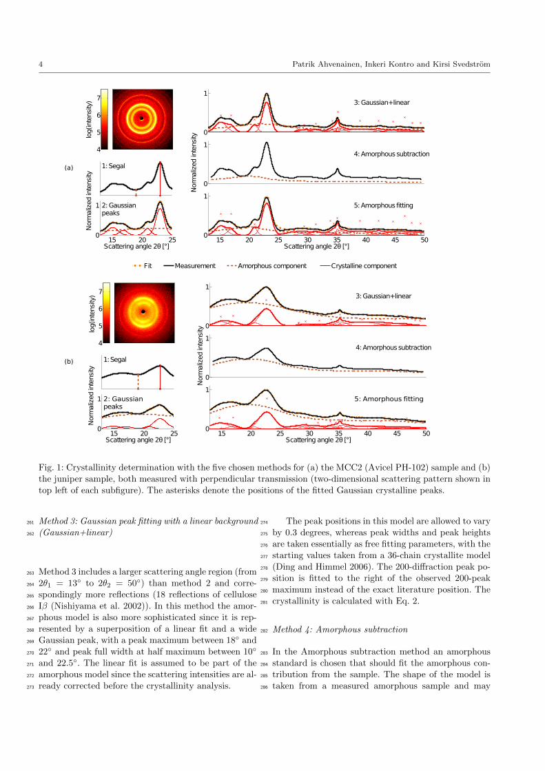
Method 1: Segal peak height231
In the Segal peak height method (Segal et al. 1959)232
a maximum intensity value I200 is found between the233
scattering angles of 2θ = 22◦ and 23◦. The region be-234
tween the cellulose Iβ 200 diffraction peak and the 110235
and 110 peaks is assumed to have very little crystalline236
contribution and is approximated as comprising of only237
an amorphous contribution. The minimum value Imin238
is taken using a minimum in the data, typically between239
2θ = 18◦ and 19◦. The sample crystallinity (usually re-240
ferred to as the crystallinity index) is then calculated241
as242
C =I200 − Imin
I200. (1)243
Method 2: Gaussian peak fitting without a linear back-244
ground (Gaussian peaks)245
In method 2 a relatively small 2θ range between 2θ1 =246
13◦ and 2θ2 = 25◦ is used and four cellulose diffraction247
peaks, corresponding to reflections 110, 110, 102 and248
200 are fitted with Gaussian peaks. A fifth Gaussian249
is fitted as the amorphous contribution. Peak positions250
for cellulose reflections are limited here to within 0.3◦ of251
the literature values (Nishiyama et al. 2002) in the least252
square fit except for the 200-diffraction peak, which is253
fitted to the right of the observed 200-peak maximum.254
The amorphous peak maximum is limited between 18◦255
and 22◦. The area of the crystalline peaks (Acr) is used256
to calculate crystallinity as257
C =Acr
Asample=
∫ 2θ22θ1
Icrd2θ∫ 2θ22θ1
Isampled2θ, (2)258
where Asample is the area under the sample intensity259
curve.260
4 Patrik Ahvenainen, Inkeri Kontro and Kirsi Svedstrom
log(intensity)
15 20 250
1
Scattering angle 2θ [°]
Normalized
intensity
0
1
0
1
Normalized
intensity
15 20 25 30 35 40 45 500
1
Scattering angle 2θ [°]
log(intensity)
4
5
6
7
Fit Measurement Amorphous component Crystalline component
log(intensity)
15 20 250
1
Scattering angle 2θ [°]
0
1
0
1
Normalized
intensity
15 20 25 30 35 40 45 500
1
Scattering angle 2θ [°]
4
5
6
7
Normalized
intensity
(b)
(a) 1:Segal
2:Gaussianpeaks
3:Gaussian+linear
4:Amorphoussubtraction
5:Amorphous fitting
3:Gaussian+linear
4:Amorphoussubtraction
2: Gaussian 5: Amorphous fittingpeaks
1:Segal
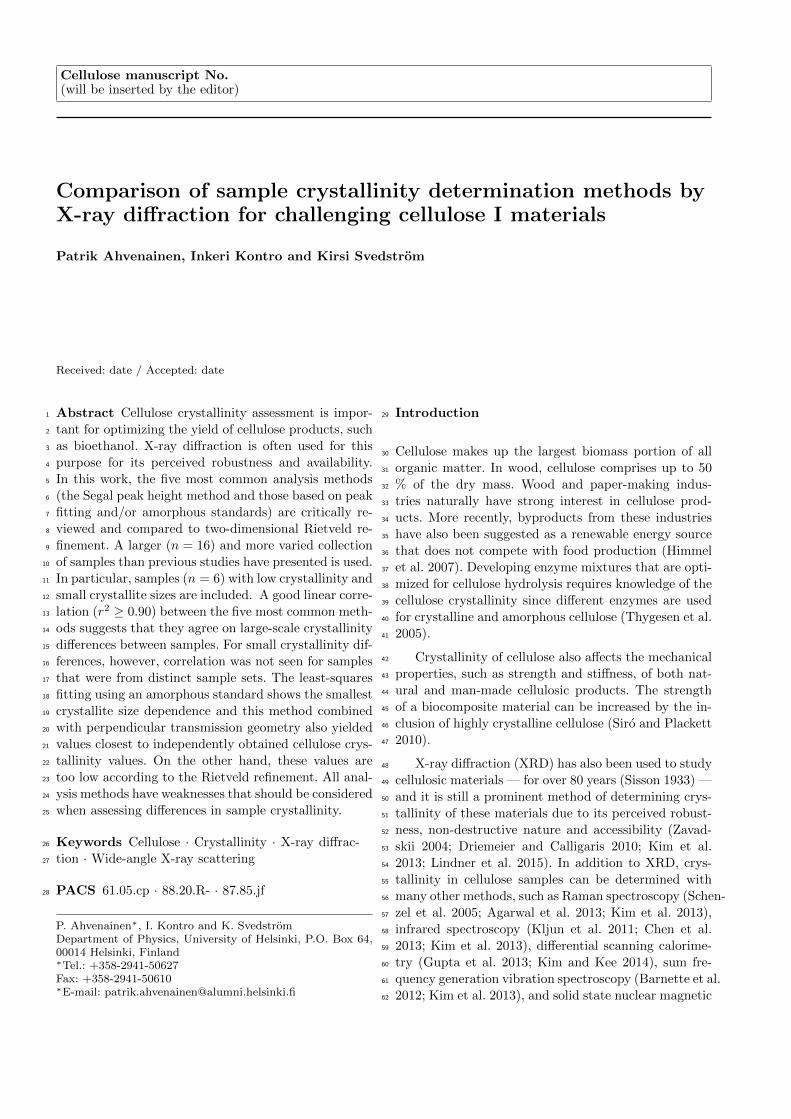
Fig. 1: Crystallinity determination with the five chosen methods for (a) the MCC2 (Avicel PH-102) sample and (b)
the juniper sample, both measured with perpendicular transmission (two-dimensional scattering pattern shown in
top left of each subfigure). The asterisks denote the positions of the fitted Gaussian crystalline peaks.
Method 3: Gaussian peak fitting with a linear background261
(Gaussian+linear)262
Method 3 includes a larger scattering angle region (from263
2θ1 = 13◦ to 2θ2 = 50◦) than method 2 and corre-264
spondingly more reflections (18 reflections of cellulose265
Iβ (Nishiyama et al. 2002)). In this method the amor-266
phous model is also more sophisticated since it is rep-267
resented by a superposition of a linear fit and a wide268
Gaussian peak, with a peak maximum between 18◦ and269
22◦ and peak full width at half maximum between 10◦270
and 22.5◦. The linear fit is assumed to be part of the271
amorphous model since the scattering intensities are al-272
ready corrected before the crystallinity analysis.273
The peak positions in this model are allowed to vary274
by 0.3 degrees, whereas peak widths and peak heights275
are taken essentially as free fitting parameters, with the276
starting values taken from a 36-chain crystallite model277
(Ding and Himmel 2006). The 200-diffraction peak po-278
sition is fitted to the right of the observed 200-peak279
maximum instead of the exact literature position. The280
crystallinity is calculated with Eq. 2.281
Method 4: Amorphous subtraction282
In the Amorphous subtraction method an amorphous283
standard is chosen that should fit the amorphous con-284
tribution from the sample. The shape of the model is285
taken from a measured amorphous sample and may286
Comparison of sample crystallinity determination methods by X-ray diffraction for challenging cellulose I materials 5
thus be more complicated and asymmetric than the287
ones of methods 2 and 3.288
Before analysis the experimental data is smoothed289
with a Gaussian filter. The amorphous curve is then fit-290
ted to the data using a constant scaling factor so that291
it touches the experimental data in at least one point292
but does not surpass it. The area under the amorphous293
curve (Aam) is then taken as the amorphous contribu-294
tion and crystallinity is then calculated as295
C = 1 − AamAsample
= 1 −∫ 2θ22θ1
Iamd2θ∫ 2θ22θ1
Isampled2θ. (3)296
The scattering angle range used to calculate the area297
is chosen to include a large wide-angle X-ray scattering298
region. Here the values of 2θ1 = 13.5◦ and 2θ2 = 49.5◦299
are used for the Amorphous subtraction method.300
Method 5: Gaussian peak fitting with an amorphous stan-301
dard (Amorphous fitting)302
Similarly to method 4, the Amorphous fitting method303
uses also an experimental amorphous standard obtained304
from a chosen amorphous sample. The crystalline model305
is the same as in method 3 and the crystallinity is cal-306
culated using Eq. 3 with 2θ1 = 13◦ and 2θ2 = 50◦. A307
linear superposition of the crystalline and amorphous308
models is used in the least squares fit. In contrast to309
method 4, method 5 features fitting which allows the310
amorphous model to surpass the measurement intensi-311
ties slightly at some scattering angles if this improves312
the fit. This can happen due to differences in the actual313
shape of the amorphous contribution and the selected314
amorphous standard.315
Comparison method: Two-dimensional Rietveld refine-316
ment317
Rietveld refinement (RR) represents a more sophisti-318
cated method of fitting crystalline cellulose peaks to319
the experimental data. RR was conducted using the320
Cellulose Rietveld analysis for fine structure (CRAFS)321
software (Oliveira and Driemeier 2013; Driemeier 2014)322
using corrected two-dimensional scattering data. The323
standard CRAFS background model was replaced with324
the linear+Gaussian amorphous model of method 3.325
Otherwise the fitting algorithm and the fitting model326
was the same as explained in Oliveira and Driemeier327
(2013). Because the samples represent cellulose from328
different sources, all the parameters for unit cell, crys-329
tallite size and diffraction peak shape were refined. The330
starting values and upper and lower boundaries for all331
these parameters were from Oliveira and Driemeier (2013)332
except for the parameters that account for differences333
15 20 25 30 35 40 45 500
0.2
0.4
0.6
0.8
1
Scattering angle 2 [!]
Nor
mal
ized
inte
nsity
!"#!"$
%#%$
&#&$
'()$*+
$
'()$*+$
110
200
110
_
!"!#
$%"$%#
,$
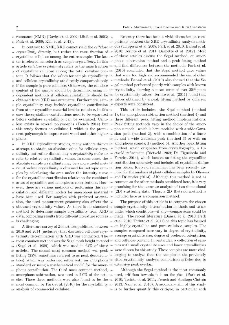
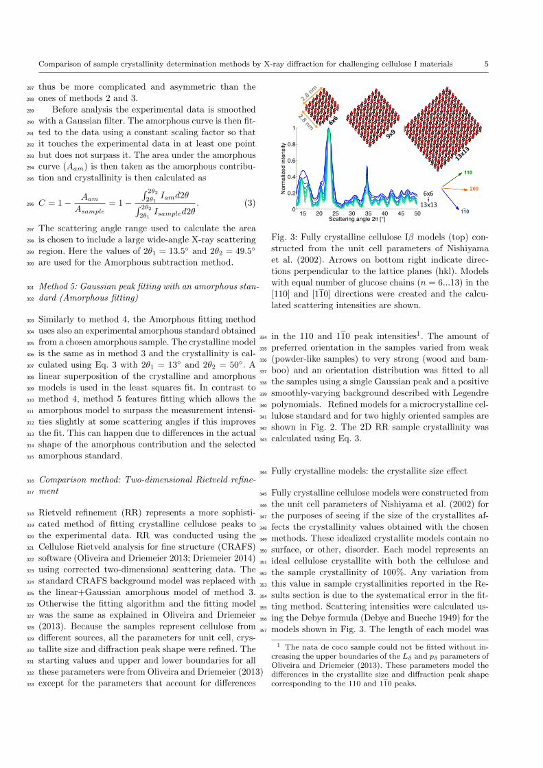
Fig. 3: Fully crystalline cellulose Iβ models (top) con-
structed from the unit cell parameters of Nishiyama
et al. (2002). Arrows on bottom right indicate direc-
tions perpendicular to the lattice planes (hkl). Models
with equal number of glucose chains (n = 6...13) in the
[110] and [110] directions were created and the calcu-
lated scattering intensities are shown.
in the 110 and 110 peak intensities1. The amount of334
preferred orientation in the samples varied from weak335
(powder-like samples) to very strong (wood and bam-336
boo) and an orientation distribution was fitted to all337
the samples using a single Gaussian peak and a positive338
smoothly-varying background described with Legendre339
polynomials. Refined models for a microcrystalline cel-340
lulose standard and for two highly oriented samples are341
shown in Fig. 2. The 2D RR sample crystallinity was342
calculated using Eq. 3.343
Fully crystalline models: the crystallite size effect344
Fully crystalline cellulose models were constructed from345
the unit cell parameters of Nishiyama et al. (2002) for346
the purposes of seeing if the size of the crystallites af-347
fects the crystallinity values obtained with the chosen348
methods. These idealized crystallite models contain no349
surface, or other, disorder. Each model represents an350
ideal cellulose crystallite with both the cellulose and351
the sample crystallinity of 100%. Any variation from352
this value in sample crystallinities reported in the Re-353
sults section is due to the systematical error in the fit-354
ting method. Scattering intensities were calculated us-355
ing the Debye formula (Debye and Bueche 1949) for the356
models shown in Fig. 3. The length of each model was357
1 The nata de coco sample could not be fitted without in-creasing the upper boundaries of the Lδ and pδ parameters ofOliveira and Driemeier (2013). These parameters model thedifferences in the crystallite size and diffraction peak shapecorresponding to the 110 and 110 peaks.
6 Patrik Ahvenainen, Inkeri Kontro and Kirsi Svedstrom
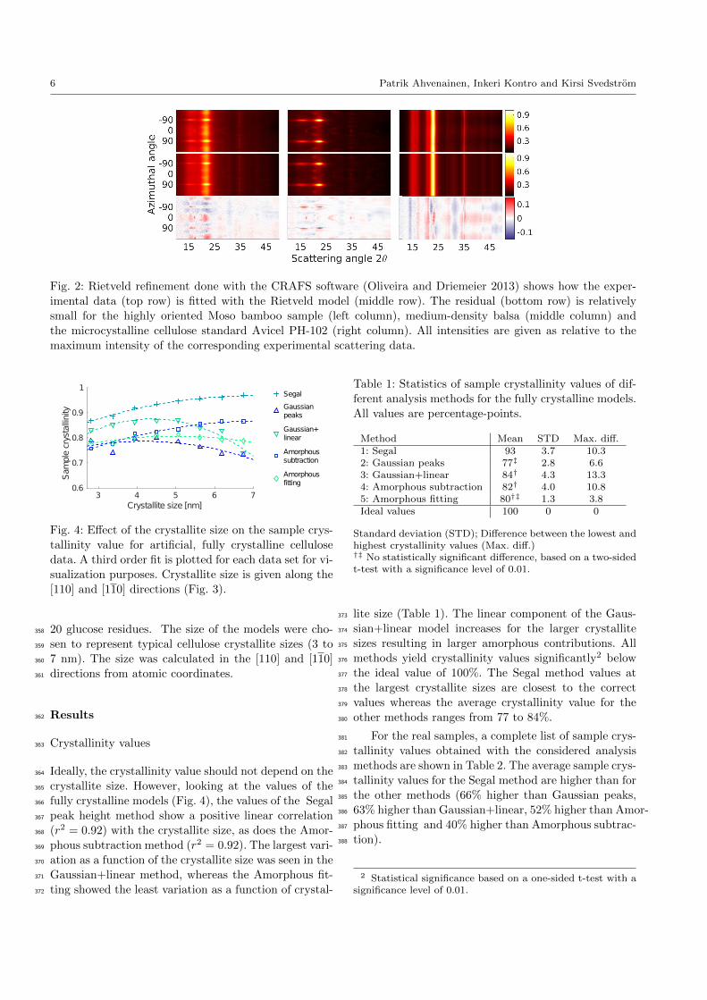
Fig. 2: Rietveld refinement done with the CRAFS software (Oliveira and Driemeier 2013) shows how the exper-
imental data (top row) is fitted with the Rietveld model (middle row). The residual (bottom row) is relatively
small for the highly oriented Moso bamboo sample (left column), medium-density balsa (middle column) and
the microcystalline cellulose standard Avicel PH-102 (right column). All intensities are given as relative to the
maximum intensity of the corresponding experimental scattering data.
Crystallite size [nm]
3 4 5 6 7
Samplecrystallinity
0.6
0.7
0.8
0.9
1Segal
Gaussianpeaks
Gaussian+linear
Amorphoussubtraction
Amorphousfitting
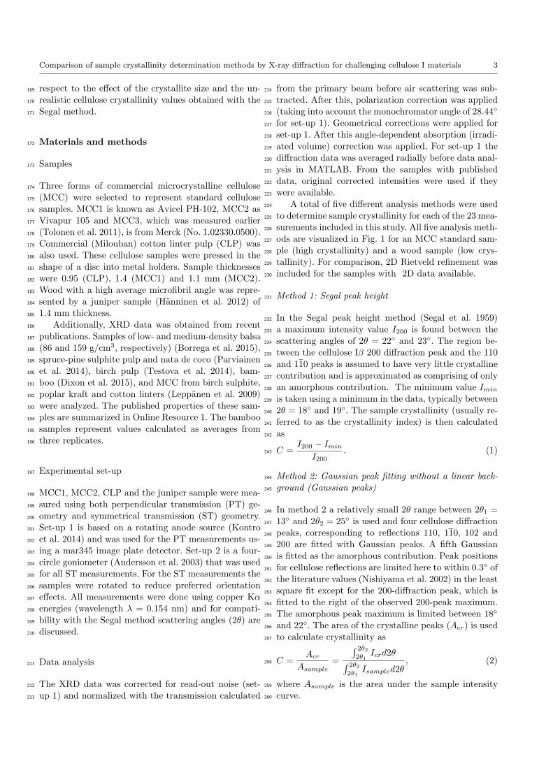
Fig. 4: Effect of the crystallite size on the sample crys-
tallinity value for artificial, fully crystalline cellulose
data. A third order fit is plotted for each data set for vi-
sualization purposes. Crystallite size is given along the
[110] and [110] directions (Fig. 3).
20 glucose residues. The size of the models were cho-358
sen to represent typical cellulose crystallite sizes (3 to359
7 nm). The size was calculated in the [110] and [110]360
directions from atomic coordinates.361
Results362
Crystallinity values363
Ideally, the crystallinity value should not depend on the364
crystallite size. However, looking at the values of the365
fully crystalline models (Fig. 4), the values of the Segal366
peak height method show a positive linear correlation367
(r2 = 0.92) with the crystallite size, as does the Amor-368
phous subtraction method (r2 = 0.92). The largest vari-369
ation as a function of the crystallite size was seen in the370
Gaussian+linear method, whereas the Amorphous fit-371
ting showed the least variation as a function of crystal-372
Table 1: Statistics of sample crystallinity values of dif-
ferent analysis methods for the fully crystalline models.
All values are percentage-points.
Method Mean STD Max. diff.1: Segal 93 3.7 10.32: Gaussian peaks 77‡ 2.8 6.63: Gaussian+linear 84† 4.3 13.34: Amorphous subtraction 82† 4.0 10.85: Amorphous fitting 80†‡ 1.3 3.8Ideal values 100 0 0
Standard deviation (STD); Difference between the lowest andhighest crystallinity values (Max. diff.)†‡ No statistically significant difference, based on a two-sidedt-test with a significance level of 0.01.
lite size (Table 1). The linear component of the Gaus-373
sian+linear model increases for the larger crystallite374
sizes resulting in larger amorphous contributions. All375
methods yield crystallinity values significantly2 below376
the ideal value of 100%. The Segal method values at377
the largest crystallite sizes are closest to the correct378
values whereas the average crystallinity value for the379
other methods ranges from 77 to 84%.380
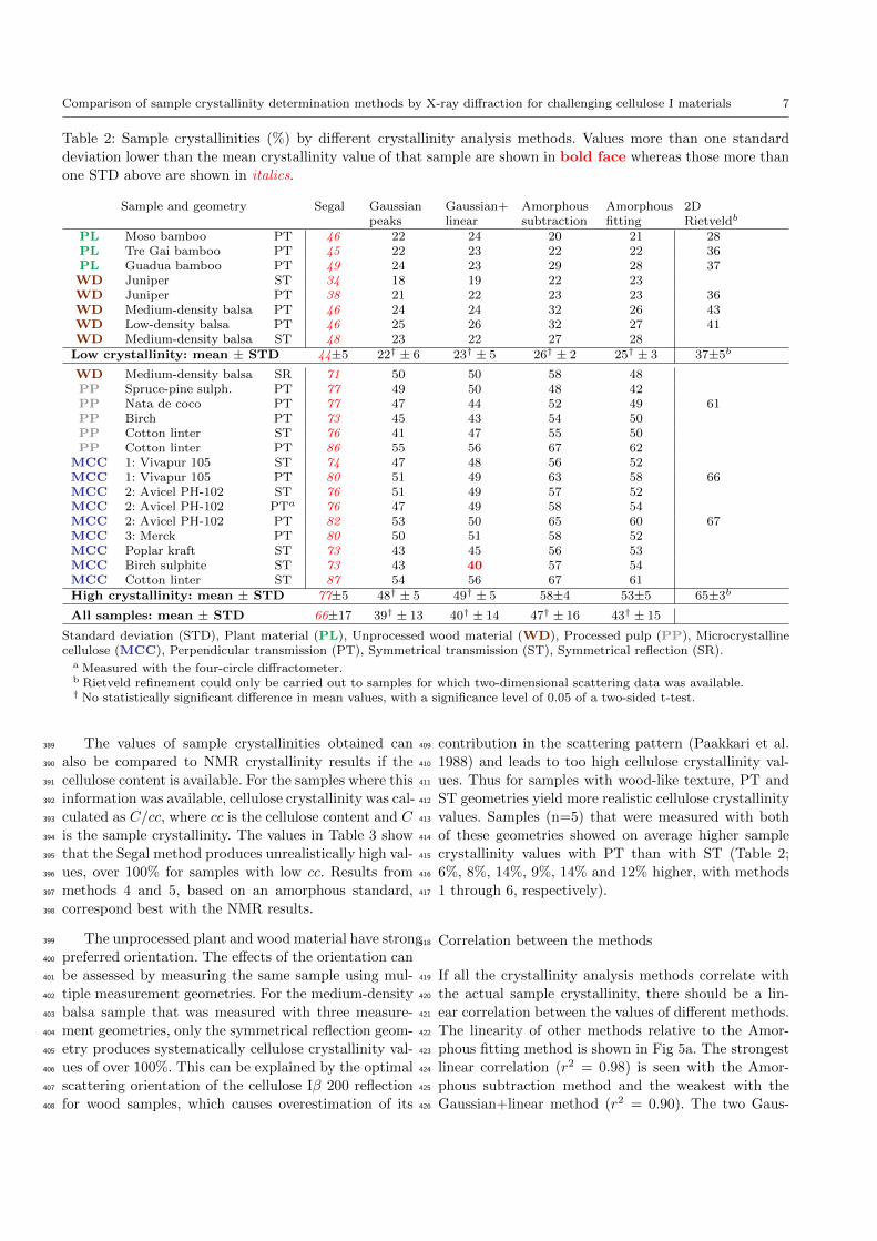
For the real samples, a complete list of sample crys-381
tallinity values obtained with the considered analysis382
methods are shown in Table 2. The average sample crys-383
tallinity values for the Segal method are higher than for384
the other methods (66% higher than Gaussian peaks,385
63% higher than Gaussian+linear, 52% higher than Amor-386
phous fitting and 40% higher than Amorphous subtrac-387
tion).388
2 Statistical significance based on a one-sided t-test with asignificance level of 0.01.
Comparison of sample crystallinity determination methods by X-ray diffraction for challenging cellulose I materials 7
Table 2: Sample crystallinities (%) by different crystallinity analysis methods. Values more than one standard
deviation lower than the mean crystallinity value of that sample are shown in bold face whereas those more than
one STD above are shown in italics.
Sample and geometry Segal Gaussianpeaks
Gaussian+linear
Amorphoussubtraction
Amorphousfitting
2DRietveldb
PL Moso bamboo PT 46 22 24 20 21 28PL Tre Gai bamboo PT 45 22 23 22 22 36PL Guadua bamboo PT 49 24 23 29 28 37WD Juniper ST 34 18 19 22 23WD Juniper PT 38 21 22 23 23 36WD Medium-density balsa PT 46 24 24 32 26 43WD Low-density balsa PT 46 25 26 32 27 41WD Medium-density balsa ST 48 23 22 27 28
Low crystallinity: mean ± STD 44±5 22† ± 6 23† ± 5 26† ± 2 25† ± 3 37±5b
WD Medium-density balsa SR 71 50 50 58 48PP Spruce-pine sulph. PT 77 49 50 48 42PP Nata de coco PT 77 47 44 52 49 61PP Birch PT 73 45 43 54 50PP Cotton linter ST 76 41 47 55 50PP Cotton linter PT 86 55 56 67 62
MCC 1: Vivapur 105 ST 74 47 48 56 52MCC 1: Vivapur 105 PT 80 51 49 63 58 66MCC 2: Avicel PH-102 ST 76 51 49 57 52MCC 2: Avicel PH-102 PTa 76 47 49 58 54MCC 2: Avicel PH-102 PT 82 53 50 65 60 67MCC 3: Merck PT 80 50 51 58 52MCC Poplar kraft ST 73 43 45 56 53MCC Birch sulphite ST 73 43 40 57 54MCC Cotton linter ST 87 54 56 67 61High crystallinity: mean ± STD 77±5 48† ± 5 49† ± 5 58±4 53±5 65±3b
All samples: mean ± STD 66±17 39† ± 13 40† ± 14 47† ± 16 43† ± 15
Standard deviation (STD), Plant material (PL), Unprocessed wood material (WD), Processed pulp (PP), Microcrystallinecellulose (MCC), Perpendicular transmission (PT), Symmetrical transmission (ST), Symmetrical reflection (SR).
a Measured with the four-circle diffractometer.b Rietveld refinement could only be carried out to samples for which two-dimensional scattering data was available.† No statistically significant difference in mean values, with a significance level of 0.05 of a two-sided t-test.
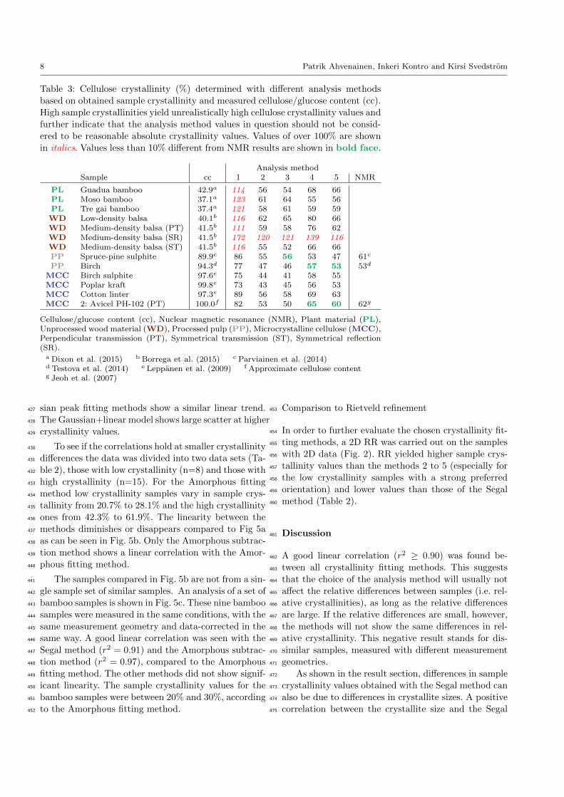
The values of sample crystallinities obtained can389
also be compared to NMR crystallinity results if the390
cellulose content is available. For the samples where this391
information was available, cellulose crystallinity was cal-392
culated as C/cc, where cc is the cellulose content and C393
is the sample crystallinity. The values in Table 3 show394
that the Segal method produces unrealistically high val-395
ues, over 100% for samples with low cc. Results from396
methods 4 and 5, based on an amorphous standard,397
correspond best with the NMR results.398
The unprocessed plant and wood material have strong399
preferred orientation. The effects of the orientation can400
be assessed by measuring the same sample using mul-401
tiple measurement geometries. For the medium-density402
balsa sample that was measured with three measure-403
ment geometries, only the symmetrical reflection geom-404
etry produces systematically cellulose crystallinity val-405
ues of over 100%. This can be explained by the optimal406
scattering orientation of the cellulose Iβ 200 reflection407
for wood samples, which causes overestimation of its408
contribution in the scattering pattern (Paakkari et al.409
1988) and leads to too high cellulose crystallinity val-410
ues. Thus for samples with wood-like texture, PT and411
ST geometries yield more realistic cellulose crystallinity412
values. Samples (n=5) that were measured with both413
of these geometries showed on average higher sample414
crystallinity values with PT than with ST (Table 2;415
6%, 8%, 14%, 9%, 14% and 12% higher, with methods416
1 through 6, respectively).417
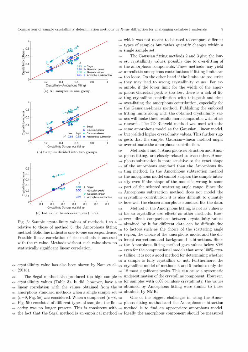
Correlation between the methods418
If all the crystallinity analysis methods correlate with419
the actual sample crystallinity, there should be a lin-420
ear correlation between the values of different methods.421
The linearity of other methods relative to the Amor-422
phous fitting method is shown in Fig 5a. The strongest423
linear correlation (r2 = 0.98) is seen with the Amor-424
phous subtraction method and the weakest with the425
Gaussian+linear method (r2 = 0.90). The two Gaus-426
8 Patrik Ahvenainen, Inkeri Kontro and Kirsi Svedstrom
Table 3: Cellulose crystallinity (%) determined with different analysis methods
based on obtained sample crystallinity and measured cellulose/glucose content (cc).
High sample crystallinities yield unrealistically high cellulose crystallinity values and
further indicate that the analysis method values in question should not be consid-
ered to be reasonable absolute crystallinity values. Values of over 100% are shown
in italics. Values less than 10% different from NMR results are shown in bold face.
Analysis methodSample cc 1 2 3 4 5 NMR
PL Guadua bamboo 42.9a 114 56 54 68 66PL Moso bamboo 37.1a 123 61 64 55 56PL Tre gai bamboo 37.4a 121 58 61 59 59WD Low-density balsa 40.1b 116 62 65 80 66WD Medium-density balsa (PT) 41.5b 111 59 58 76 62WD Medium-density balsa (SR) 41.5b 172 120 121 139 116WD Medium-density balsa (ST) 41.5b 116 55 52 66 66PP Spruce-pine sulphite 89.9c 86 55 56 53 47 61c
PP Birch 94.3d 77 47 46 57 53 53d
MCC Birch sulphite 97.6e 75 44 41 58 55MCC Poplar kraft 99.8e 73 43 45 56 53MCC Cotton linter 97.3e 89 56 58 69 63MCC 2: Avicel PH-102 (PT) 100.0f 82 53 50 65 60 62g
Cellulose/glucose content (cc), Nuclear magnetic resonance (NMR), Plant material (PL),Unprocessed wood material (WD), Processed pulp (PP), Microcrystalline cellulose (MCC),Perpendicular transmission (PT), Symmetrical transmission (ST), Symmetrical reflection(SR).
a Dixon et al. (2015) b Borrega et al. (2015) c Parviainen et al. (2014)d Testova et al. (2014) e Leppanen et al. (2009) f Approximate cellulose contentg Jeoh et al. (2007)
sian peak fitting methods show a similar linear trend.427
The Gaussian+linear model shows large scatter at higher428
crystallinity values.429
To see if the correlations hold at smaller crystallinity430
differences the data was divided into two data sets (Ta-431
ble 2), those with low crystallinity (n=8) and those with432
high crystallinity (n=15). For the Amorphous fitting433
method low crystallinity samples vary in sample crys-434
tallinity from 20.7% to 28.1% and the high crystallinity435
ones from 42.3% to 61.9%. The linearity between the436
methods diminishes or disappears compared to Fig 5a437
as can be seen in Fig. 5b. Only the Amorphous subtrac-438
tion method shows a linear correlation with the Amor-439
phous fitting method.440
The samples compared in Fig. 5b are not from a sin-441
gle sample set of similar samples. An analysis of a set of442
bamboo samples is shown in Fig. 5c. These nine bamboo443
samples were measured in the same conditions, with the444
same measurement geometry and data-corrected in the445
same way. A good linear correlation was seen with the446
Segal method (r2 = 0.91) and the Amorphous subtrac-447
tion method (r2 = 0.97), compared to the Amorphous448
fitting method. The other methods did not show signif-449
icant linearity. The sample crystallinity values for the450
bamboo samples were between 20% and 30%, according451
to the Amorphous fitting method.452
Comparison to Rietveld refinement453
In order to further evaluate the chosen crystallinity fit-454
ting methods, a 2D RR was carried out on the samples455
with 2D data (Fig. 2). RR yielded higher sample crys-456
tallinity values than the methods 2 to 5 (especially for457
the low crystallinity samples with a strong preferred458
orientation) and lower values than those of the Segal459
method (Table 2).460
Discussion461
A good linear correlation (r2 ≥ 0.90) was found be-462
tween all crystallinity fitting methods. This suggests463
that the choice of the analysis method will usually not464
affect the relative differences between samples (i.e. rel-465
ative crystallinities), as long as the relative differences466
are large. If the relative differences are small, however,467
the methods will not show the same differences in rel-468
ative crystallinity. This negative result stands for dis-469
similar samples, measured with different measurement470
geometries.471
As shown in the result section, differences in sample472
crystallinity values obtained with the Segal method can473
also be due to differences in crystallite sizes. A positive474
correlation between the crystallite size and the Segal475
Comparison of sample crystallinity determination methods by X-ray diffraction for challenging cellulose I materials 9
Crystallinity (Amorphous fitting)
0 0.2 0.4 0.6 0.8 1
Crystallinity(others)
0
0.2
0.4
0.6
0.8
1
0.93
0.910.900.98
Segal
Gaussian peaks
Gaussian+linear
Amorphous subtraction
r2
(a) All samples in one group.
Crystallinity (Amorphous fitting)
0 0.2 0.4 0.6 0.8 1
Crystallinity(others)
0
0.2
0.4
0.6
0.8
1
0.64 0.88
Segal
Gaussian peaks
Gaussian+linear
Amorphous subtraction
low
r2
high
(b) Samples divided into two groups.
Crystallinity (Amorphous fitting)
0 0.1 0.2 0.3 0.4 0.5 0.6 0.7
Crystallinity(others)
0
0.1
0.2
0.3
0.4
0.5
0.6
0.910.50
0.97
Segal
Gaussian peaks
Gaussian+linear
Amorphous subtraction
r2
(c) Individual bamboo samples (n=9).
Fig. 5: Sample crystallinity values of methods 1 to 4
relative to those of method 5, the Amorphous fitting
method. Solid line indicates one-to-one correspondence.
Possible linear correlation of the methods is assessed
with the r2 value. Methods without such value show no
statistically significant linear correlation.
crystallinity value has also been shown by Nam et al.476
(2016).477
The Segal method also produced too high sample478
crystallinity values (Table 3). It did, however, have a479
linear correlation with the values obtained from the480
amorphous standard methods when a single sample set481
(n=9, Fig. 5c) was considered. When a sample set (n=8,482
Fig. 5b) consisted of different types of samples, the lin-483
earity was no longer present. This is consistent with484
the fact that the Segal method is an empirical method485
which was not meant to be used to compare different486
types of samples but rather quantify changes within a487
single sample set.488
The Gaussian fitting methods 2 and 3 give the low-489
est crystallinity values, possibly due to over-fitting of490
the amorphous components. These methods may yield491
unrealistic amorphous contributions if fitting limits are492
too loose. On the other hand if the limits are too strict493
they may lead to wrong crystallinity values. For ex-494
ample, if the lower limit for the width of the amor-495
phous Gaussian peak is too low, there is a risk of fit-496
ting crystalline contribution with this peak and thus497
over-fitting the amorphous contribution, especially for498
the Gaussian+linear method. Publishing the enforced499
fitting limits along with the obtained crystallinity val-500
ues will make these results more comparable with other501
research. The 2D Rietveld method was used with the502
same amorphous model as the Gaussian+linear model,503
but yielded higher crystallinity values. This further sug-504
gests that the simpler Gaussian+linear method might505
overestimate the amorphous contribution.506
Methods 4 and 5, Amorphous subtraction and Amor-507
phous fitting, are closely related to each other. Amor-508
phous subtraction is more sensitive to the exact shape509
of the amorphous standard than the Amorphous fit-510
ting method. In the Amorphous subtraction method511
the amorphous model cannot surpass the sample inten-512
sity even if the shape of the model is wrong in some513
part of the selected scattering angle range. Since the514
Amorphous subtraction method does not model the515
crystalline contribution it is also difficult to quantify516
how well the chosen amorphous standard fits the data.517
Method 5, the Amorphous fitting, is not as vulnera-518
ble to crystallite size effects as other methods. How-519
ever, direct comparisons between crystallinity values520
obtained by it for different data can be difficult due521
to factors such as the choice of the scattering angle522
region, the choice of the amorphous model and the dif-523
ferent corrections and background subtractions. Since524
the Amorphous fitting method gave values below 80%525
even for the computational models that were 100% crys-526
talline, it is not a good method for determining whether527
a sample is fully crystalline or not. Furthermore, the528
crystalline model of methods 3 and 5 includes only the529
18 most significant peaks. This can cause a systematic530
underestimation of the crystalline component. However,531
for samples with 60% cellulose crystallinity, the values532
obtained by Amorphous fitting were similar to those533
obtained by NMR.534
One of the biggest challenges in using the Amor-535
phous fitting method and the Amorphous subtraction536
method is to find an appropriate amorphous model.537
Ideally the amorphous component should be measured538
10 Patrik Ahvenainen, Inkeri Kontro and Kirsi Svedstrom
Scattering angle 2 θ [°]
10 15 20 25 30 35 40 45 50
Normalizedintensity[arb.units]
0
0.5
1
1.5
2(a) Beechwood organosolv lignin
(b) Arabinoxylan
(c) Glucomannan
(d) Sulphate lignin
(e) Ball-milled cellulose
c
e
d
b
a
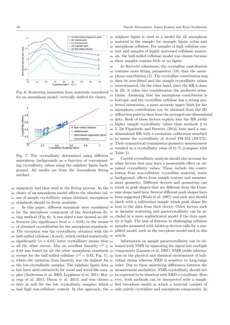
Fig. 6: Scattering intensities from materials considered
for an amorphous model, vertically shifted for clarity.
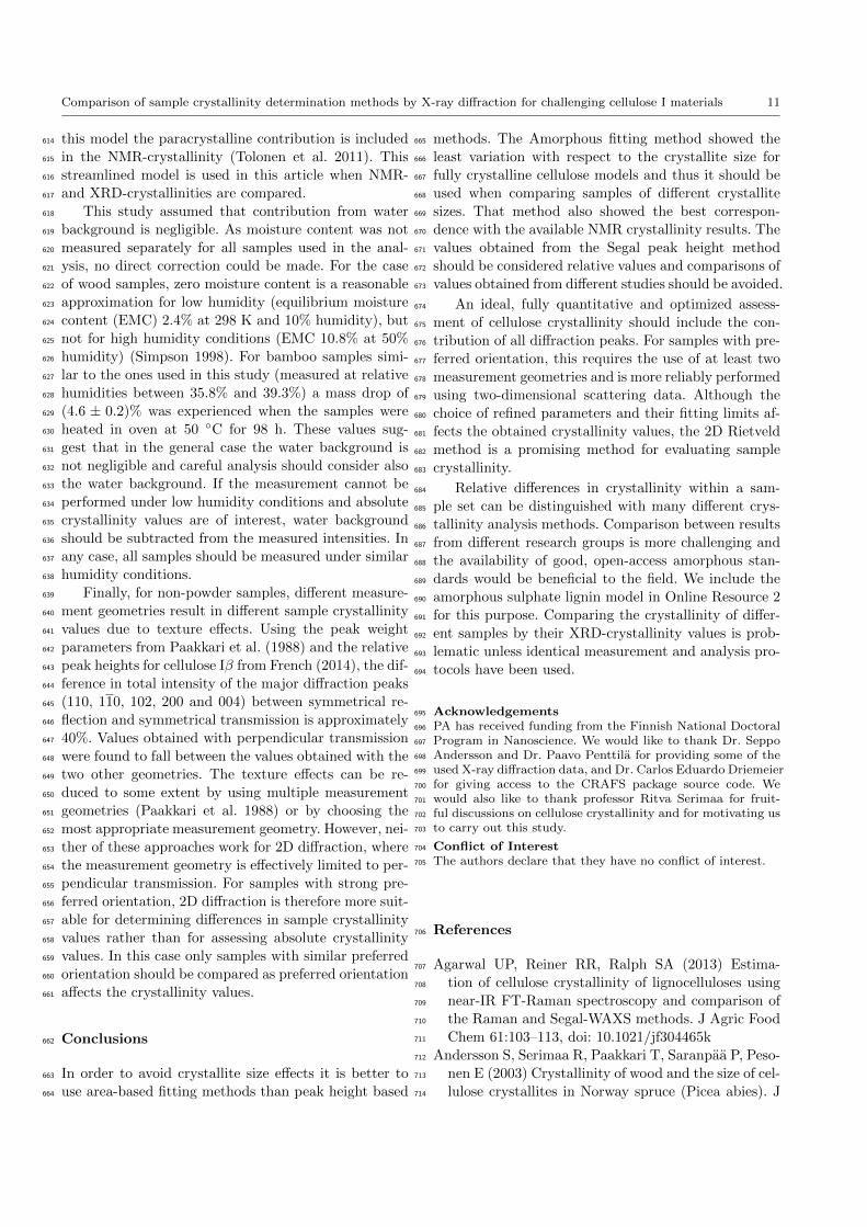
0 0.2 0.4 0.6 0.8 10
0.2
0.4
0.6
0.8
1
Crystallinity (Sulphate lignin)
Crystallinity(others)
r2=0.82r2=0.97
r2=0.95r2=0.94
Ball−milled cellulose
arabinoxylan
Beechwood organosolv lignin
Glucomannan
Fig. 7: The crystallinity determined using different
amorphous backgrounds as a function of correspond-
ing crystallinity values using the sulphate lignin back-
ground. All results are from the Amorphous fitting
method.
separately and then used in the fitting process. As the539
choice of an amorphous model affects the absolute val-540
ues of sample crystallinity values obtained, amorphous541
standards should be freely available.542
In this paper, different standards were considered543
for the amorphous component of the Amorphous fit-544
ting method (Fig. 6). A two-sided t-test showed no dif-545
ferences (for significance level α = 0.05) in the means546
of obtained crystallinities for the amorphous standards.547
The exception was the crystallinity obtained with the548
ball-milled cellulose (Avicel), which yielded statistically549
significantly (α = 0.01) lower crystallinity means than550
all the other curves. Also an excellent linearity r2 ≥551
0.94 was found for all the other amorphous standards552
except for the ball-milled cellulose (r2 = 0.82, Fig. 7),553
where the variation from linearity was the highest for554
the low-crystallinity samples. The sulphate lignin data555
has been used extensively for wood and wood-like sam-556
ples (Andersson et al. 2003; Leppanen et al. 2011; Bor-557
rega et al. 2015; Dixon et al. 2015) and was chosen558
here as well for the low crystallinity samples, which559
had high non-cellulosic content. In this approach, the560
sulphate lignin is used as a model for all amorphous561
material in the sample: for example lignin, xylan and562
amorphous cellulose. For samples of high cellulose con-563
tent and samples of highly processed cellulosic materi-564
als, the ball-milled cellulose model was chosen because565
these samples contain little or no lignin.566
In Rietveld refinement, the crystalline contribution567
contains more fitting parameters (18) than the amor-568
phous contribution (5). The crystalline contribution may569
then be over-fitted and the sample crystallinity values570
overestimated. On the other hand, since the RR is done571
in 2D, it takes into consideration the preferred orien-572
tation. Assuming that the amorphous contribution is573
isotropic and the crystalline cellulose has a strong pre-574
ferred orientation, a more accurate upper limit for the575
amorphous contribution can be obtained from the 2D576
diffraction pattern than from the averaged one-dimensional577
data. Both of these factors explain why the RR yields578
higher sample crystallinity values than methods 2 to579
5. De Figueiredo and Ferreira (2014) have used a one-580
dimensional RR with a corundum calibration standard581
to assess the crystallinity of Avicel PH-102 (MCC2).582
Their symmetrical transmission geometry measurement583
resulted in a crystallinity value of 51 % (compare with584
Table 2).585
Careful crystallinity analysis should also account for586
other factors that may have a measurable effect on ob-587
tained crystallinity values. These include the contri-588
bution from non-cellulosic crystalline material, water589
background, effects from sample texture and measure-590
ment geometry. Different devices and geometries can591
result in peak shapes that are different from the Gaus-592
sian shape used here. Several different peak shapes have593
been suggested (Wada et al. 1997) and each user should594
check with a calibration sample which peak shape fits595
best to the data from their device. Other factors such596
as inelastic scattering and paracrystallinity can be in-597
cluded in a more sophisticated model if the data qual-598
ity is high. The lack of features in challenging cellulose599
samples measured with tabletop devices calls for a sim-600
plified model, such as the two-phase model used in this601
article.602
Information on sample paracrystallinity can be ob-603
tained with NMR by separating the signal into multiple604
components (Larsson et al. 1997). NMR yields informa-605
tion on the physical and chemical environment of indi-606
vidual atoms whereas XRD is sensitive to long-range607
order. Due to these underlying differences between the608
measurement modalities, NMR-crystallinity should not609
be expected to be identical with XRD-crystallinity. How-610
ever, both methods can be interpreted with a simpli-611
fied two-phase model in which a material consists of612
only purely crystalline and amorphous components. In613
Comparison of sample crystallinity determination methods by X-ray diffraction for challenging cellulose I materials 11
this model the paracrystalline contribution is included614
in the NMR-crystallinity (Tolonen et al. 2011). This615
streamlined model is used in this article when NMR-616
and XRD-crystallinities are compared.617
This study assumed that contribution from water618
background is negligible. As moisture content was not619
measured separately for all samples used in the anal-620
ysis, no direct correction could be made. For the case621
of wood samples, zero moisture content is a reasonable622
approximation for low humidity (equilibrium moisture623
content (EMC) 2.4% at 298 K and 10% humidity), but624
not for high humidity conditions (EMC 10.8% at 50%625
humidity) (Simpson 1998). For bamboo samples simi-626
lar to the ones used in this study (measured at relative627
humidities between 35.8% and 39.3%) a mass drop of628
(4.6 ± 0.2)% was experienced when the samples were629
heated in oven at 50 ◦C for 98 h. These values sug-630
gest that in the general case the water background is631
not negligible and careful analysis should consider also632
the water background. If the measurement cannot be633
performed under low humidity conditions and absolute634
crystallinity values are of interest, water background635
should be subtracted from the measured intensities. In636
any case, all samples should be measured under similar637
humidity conditions.638
Finally, for non-powder samples, different measure-639
ment geometries result in different sample crystallinity640
values due to texture effects. Using the peak weight641
parameters from Paakkari et al. (1988) and the relative642
peak heights for cellulose Iβ from French (2014), the dif-643
ference in total intensity of the major diffraction peaks644
(110, 110, 102, 200 and 004) between symmetrical re-645
flection and symmetrical transmission is approximately646
40%. Values obtained with perpendicular transmission647
were found to fall between the values obtained with the648
two other geometries. The texture effects can be re-649
duced to some extent by using multiple measurement650
geometries (Paakkari et al. 1988) or by choosing the651
most appropriate measurement geometry. However, nei-652
ther of these approaches work for 2D diffraction, where653
the measurement geometry is effectively limited to per-654
pendicular transmission. For samples with strong pre-655
ferred orientation, 2D diffraction is therefore more suit-656
able for determining differences in sample crystallinity657
values rather than for assessing absolute crystallinity658
values. In this case only samples with similar preferred659
orientation should be compared as preferred orientation660
affects the crystallinity values.661
Conclusions662
In order to avoid crystallite size effects it is better to663
use area-based fitting methods than peak height based664
methods. The Amorphous fitting method showed the665
least variation with respect to the crystallite size for666
fully crystalline cellulose models and thus it should be667
used when comparing samples of different crystallite668
sizes. That method also showed the best correspon-669
dence with the available NMR crystallinity results. The670
values obtained from the Segal peak height method671
should be considered relative values and comparisons of672
values obtained from different studies should be avoided.673
An ideal, fully quantitative and optimized assess-674
ment of cellulose crystallinity should include the con-675
tribution of all diffraction peaks. For samples with pre-676
ferred orientation, this requires the use of at least two677
measurement geometries and is more reliably performed678
using two-dimensional scattering data. Although the679
choice of refined parameters and their fitting limits af-680
fects the obtained crystallinity values, the 2D Rietveld681
method is a promising method for evaluating sample682
crystallinity.683
Relative differences in crystallinity within a sam-684
ple set can be distinguished with many different crys-685
tallinity analysis methods. Comparison between results686
from different research groups is more challenging and687
the availability of good, open-access amorphous stan-688
dards would be beneficial to the field. We include the689
amorphous sulphate lignin model in Online Resource 2690
for this purpose. Comparing the crystallinity of differ-691
ent samples by their XRD-crystallinity values is prob-692
lematic unless identical measurement and analysis pro-693
tocols have been used.694
Acknowledgements695
PA has received funding from the Finnish National Doctoral696
Program in Nanoscience. We would like to thank Dr. Seppo697
Andersson and Dr. Paavo Penttila for providing some of the698
used X-ray diffraction data, and Dr. Carlos Eduardo Driemeier699
for giving access to the CRAFS package source code. We700
would also like to thank professor Ritva Serimaa for fruit-701
ful discussions on cellulose crystallinity and for motivating us702
to carry out this study.703
Conflict of Interest704
The authors declare that they have no conflict of interest.705
References706
Agarwal UP, Reiner RR, Ralph SA (2013) Estima-707
tion of cellulose crystallinity of lignocelluloses using708
near-IR FT-Raman spectroscopy and comparison of709
the Raman and Segal-WAXS methods. J Agric Food710
Chem 61:103–113, doi: 10.1021/jf304465k711
Andersson S, Serimaa R, Paakkari T, Saranpaa P, Peso-712
nen E (2003) Crystallinity of wood and the size of cel-713
lulose crystallites in Norway spruce (Picea abies). J714
12 Patrik Ahvenainen, Inkeri Kontro and Kirsi Svedstrom
Wood Sci 49:531–537, doi: 10.1007/s10086-003-0518-715
x716
Bansal P, Hall M, Realff MJ, Lee JH, Bommarius717
AS (2010) Multivariate statistical analysis of X-718
ray data from cellulose: A new method to deter-719
mine degree of crystallinity and predict hydroly-720
sis rates. Bioresour Technol 101:4461–4471, doi:721
10.1016/j.biortech.2010.01.068722
Barnette AL, Lee C, Bradley LC, Schreiner EP, Park723
YB, Shin H, Cosgrove DJ, Park S, Kim SH (2012)724
Quantification of crystalline cellulose in lignocellu-725
losic biomass using sum frequency generation (SFG)726
vibration spectroscopy and comparison with other727
analytical methods. Carbohydr Polym 89:802–809,728
doi: 10.1016/j.carbpol.2012.04.014729
Borrega M, Ahvenainen P, Serimaa R, Gibson L (2015)730
Composition and structure of balsa (Ochroma pyra-731
midale) wood. Wood Sci Technol 49:403–420, doi:732
10.1007/s00226-015-0700-5733
Chen C, Luo J, Qin W, Tong Z (2013) Elemental734
analysis, chemical composition, cellulose crystallinity,735
and FT-IR spectra of Toona sinensis wood. Monat-736
shefte fur Chemie - Chem Mon 145:175–185, doi:737
10.1007/s00706-013-1077-5738
Davies LM, Harris PJ, Newman RH (2002) Molecular739
ordering of cellulose after extraction of polysaccha-740
rides from primary cell walls of Arabidopsis thaliana:741
a solid-state CP/MAS (13)C NMR study. Carbohydr742
Res 337:587–93, doi: 10.1016/S0008-6215(02)00038-1743
De Figueiredo LP, Ferreira FF (2014) The Rietveld744
Method as a Tool to Quantify the Amorphous745
Amount of Microcrystalline Cellulose. J Pharm Sci746
pp 1394–1399, doi: 10.1002/jps.23909747
Debye P, Bueche AM (1949) Scattering by an in-748
homogeneous solid. J Appl Phys 20:518–525, doi:749
10.1063/1.1698419750
Ding SY, Himmel ME (2006) The maize primary cell751
wall microfibril: a new model derived from direct vi-752
sualization. J Agric Food Chem 54:597–606, doi:753
10.1021/jf051851z754
Dixon P, Ahvenainen P, Aijazi A, Chen S, Lin755
S, Augusciak P, Borrega M, Svedstrom K, Gib-756
son L (2015) Comparison of the structure and757
flexural properties of Moso, Guadua and Tre758
Gai bamboo. Constr Build Mater 90:11–17, doi:759
10.1016/j.conbuildmat.2015.04.042760
Driemeier C (2014) Two-dimensional Rietveld analysis761
of celluloses from higher plants. Cellulose 21:1065–762
1073, doi: 10.1007/s10570-013-9995-2763
Driemeier C, Calligaris GA (2010) Theoretical and ex-764
perimental developments for accurate determination765
of crystallinity of cellulose I materials. J Appl Crys-766
tallogr 44:184–192, doi: 10.1107/S0021889810043955767
French AD (2014) Idealized powder diffraction patterns768
for cellulose polymorphs. Cellulose 21:885–896, doi:769
10.1007/s10570-013-0030-4770
French AD, Santiago Cintron M (2013) Cellulose poly-771
morphy, crystallite size, and the Segal Crystallinity772
Index. Cellulose 20:583–588, doi: 10.1007/s10570-773
012-9833-y774
Gupta B, Agarwal R, Sarwar Alam M (2013) Prepa-775
ration and characterization of polyvinyl alcohol-776
polyethylene oxide-carboxymethyl cellulose blend777
membranes. J Appl Polym Sci 127:1301–1308, doi:778
10.1002/app.37665779
Hanninen T, Tukiainen P, Svedstrom K, Serimaa780
R, Saranpaa P, Kontturi E, Hughes M, Vuorinen781
T (2012) Ultrastructural evaluation of compression782
wood-like properties of common juniper (Junipe-783
rus communis L.). Holzforschung 66:389–395, doi:784
10.1515/hf.2011.166785
Himmel ME, Ding SY, Johnson DK, Adney WS, Nim-786
los MR, Brady JW, Foust TD (2007) Biomass Re-787
calcitrance: Engineering Plants and Enzymes for788
Biofuels Production. Science 315:804–807, doi:789
10.1126/science.1137016790
Jeoh T, Ishizawa CI, Davis MF, Himmel ME, Ad-791
ney WS, Johnson DK (2007) Cellulase digestibil-792
ity of pretreated biomass is limited by cellulose793
accessibility. Biotechnol Bioeng 98:112–122, doi:794
10.1002/bit.21408795
Kim SH, Lee CM, Kafle K (2013) Characterization of796
crystalline cellulose in biomass: Basic principles, ap-797
plications, and limitations of XRD, NMR, IR, Ra-798
man, and SFG. Korean J Chem Eng 30:2127–2141,799
doi: 10.1007/s11814-013-0162-0800
Kim SS, Kee CD (2014) Electro-active polymer actu-801
ator based on PVDF with bacterial cellulose nano-802
whiskers (BCNW) via electrospinning method. Int J803
Precis Eng Manuf 15:315–321, doi: 10.1007/s12541-804
014-0340-y805
Kljun A, Benians TAS, Goubet F, Meulewaeter F,806
Knox JP, Blackburn RS (2011) Comparative analy-807
sis of crystallinity changes in cellulose I polymers us-808
ing ATR-FTIR, X-ray diffraction, and carbohydrate-809
binding module probes. Biomacromolecules 12:4121–810
4126, doi: 10.1021/bm201176m811
Kontro I, Wiedmer SK, Hynonen U, Penttila PA,812
Palva A, Serimaa R (2014) The structure of Lac-813
tobacillus brevis surface layer reassembled on lipo-814
somes differs from native structure as revealed by815
SAXS. Biochim Biophys Acta 1838:2099–104, doi:816
10.1016/j.bbamem.2014.04.022817
Larsson PT, Wickholm K, Iversen T (1997) A CP /818
MAS 13C NMR investigation of molecular order-819
ing in celluloses. Carbohydr Res 302:19–25, doi:820
Comparison of sample crystallinity determination methods by X-ray diffraction for challenging cellulose I materials 13
10.1016/S0008-6215(97)00130-4821
Leppanen K, Andersson S, Torkkeli M, Knaapila M,822
Kotelnikova N, Serimaa R (2009) Structure of cellu-823
lose and microcrystalline cellulose from various wood824
species, cotton and flax studied by X-ray scatter-825
ing. Cellulose 16:999–1015, doi: 10.1007/s10570-009-826
9298-9827
Leppanen K, Bjurhager I, Peura M, Kallonen A, Suuro-828
nen JP, Penttila PA, Love J, Fagerstedt K, Serimaa R829
(2011) X-ray scattering and microtomography study830
on the structural changes of never-dried silver birch,831
European aspen and hybrid aspen during drying.832
Holzforschung 65:865–873, doi: 10.1515/HF.2011.108833
Liitia T, Maunu SL, Hortling B, Tamminen T, Pekkala834
O, Varhimo A, Liiti T, Varhimo A (2003) Cellu-835
lose crystallinity and ordering of hemicelluloses in836
pine and birch pulps as revealed by solid-state NMR837
spectroscopic methods. Cellulose 10:307–316, doi:838
10.1023/A:1027302526861839
Lindner B, Petridis L, Langan P, Smith JC (2015)840
Determination of cellulose crystallinity from powder841
diffraction diagrams. Biopolymers 103:67–73, doi:842
10.1002/bip.22555843
Nam S, French AD, Condon BD, Concha M (2016)844
Segal crystallinity index revisited by the simulation845
of X-ray diffraction patterns of cotton cellulose Iβ846
and cellulose II. Carbohydr Polym 135:1–9, doi:847
10.1016/j.carbpol.2015.08.035848
Nishiyama Y, Langan P, Chanzy H (2002) Crystal849
structure and hydrogen-bonding system in cellu-850
lose Iβ from synchrotron X-ray and neutron fiber851
diffraction. J Am Chem Soc 124:9074–9082, doi:852
10.1021/ja0257319853
Oliveira RP, Driemeier C (2013) CRAFS: A model to854
analyze two-dimensional X-ray diffraction patterns of855
plant cellulose. J Appl Crystallogr 46:1196–1210, doi:856
10.1107/S0021889813014805857
Paakkari T, Blomberg M, Serimaa R, Jarvinen M858
(1988) A texture correction for quantitative X-ray859
powder diffraction analysis of cellulose. J Appl Crys-860
tallogr 21:393–397, doi: 10.1107/S0021889888003371861
Park S, Johnson DK, Ishizawa CI, Parilla PA, Davis862
MF (2009) Measuring the crystallinity index of cel-863
lulose by solid state 13C nuclear magnetic resonance.864
Cellulose 16:641–647, doi: 10.1007/s10570-009-9321-865
1866
Park S, Baker JO, Himmel ME, Parilla PA, John-867
son DK (2010) Cellulose crystallinity index: mea-868
surement techniques and their impact on interpreting869
cellulase performance. Biotechnol Biofuels 3:10, doi:870
10.1186/1754-6834-3-10871
Parviainen H, Parviainen A, Virtanen T, Kilpelainen I,872
Ahvenainen P, Serimaa R, Gronqvist S, Maloney T,873
Maunu SL (2014) Dissolution enthalpies of cellulose874
in ionic liquids. Carbohydr Polym 113:67–76, doi:875
10.1016/j.carbpol.2014.07.001876
Rietveld HM (1969) A profile refinement method for877
nuclear and magnetic structures. J Appl Crystallogr878
2:65–71, doi: 10.1107/S0021889869006558879
Schenzel K, Fischer S, Brendler E (2005) New Method880
for Determining the Degree of Cellulose I Crys-881
tallinity by Means of FT Raman Spectroscopy. Cel-882
lulose 12:223–231, doi: 10.1007/s10570-004-3885-6883
Segal L, Creely J, Martin A, Conrad C (1959)884
An Empirical Method for Estimating the Degree885
of Crystallinity of Native Cellulose Using the X-886
Ray Diffractometer. Text Res J 29:786–794, doi:887
10.1177/004051755902901003888
Simpson WT (1998) Equilibrium Moisture Content of889
Wood in Outdoor Locations in the United States and890
Worldwide. Tech. rep., U.S. Department of Agricul-891
ture, Forest Service, Forest Products Laboratory892
Siro I, Plackett D (2010) Microfibrillated cellulose and893
new nanocomposite materials: A review. Cellulose894
17:459–494, doi: 10.1007/s10570-010-9405-y895
Sisson WA (1933) X-Ray Analysis of Fibers. Part I,896
Literature Survey. Text Res J 3:295–307897
Terinte N, Ibbett R, Schuster KC (2011) Overview898
on Native Cellulose and Microcrystalline Cellu-899
lose I Structure Studied By X-Ray Diffraction900
(WAXD): Comparison Between Measurement Tech-901
niques. Lenzinger Berichte 89:118–131902
Testova L, Borrega M, Tolonen LK, Penttila PA, Seri-903
maa R, Larsson PT, Sixta H (2014) Dissolving-grade904
birch pulps produced under various prehydrolysis in-905
tensities: quality, structure and applications. Cellu-906
lose 21:2007–2021, doi: 10.1007/s10570-014-0182-x907
Thygesen A, Oddershede J, Lilholt H, Thomsen AB,908
Stahl K (2005) On the determination of crystallinity909
and cellulose content in plant fibres. Cellulose 12:563–910
576, doi: 10.1007/s10570-005-9001-8911
Tolonen LK, Zuckerstatter G, Penttila PA, Milacher912
W, Habicht W, Serimaa R, Kruse A, Sixta H913
(2011) Structural changes in microcrystalline cel-914
lulose in subcritical water treatment. Biomacro-915
molecules 12:2544–51, doi: 10.1021/bm200351y916
Wada M, Okano T, Sugiyama J (1997) Synchrotron-917
radiated X-ray and neutron diffraction study of na-918
tive cellulose. Cellulose 4:221–232919
Zavadskii AE (2004) X-ray diffraction method of deter-920
mining the degree of crystallinity of cellulose mate-921
rials of different anisotropy. Fibre Chem 36:425–430,922
doi: 10.1007/s10692-005-0031-7923
Recommended