J. Agr. Sci. Tech. (2016) Vol. 18: 681-694
681
Comparative Evaluation of Neural Network and Regression
Based Models to Simulate Runoff and Sediment Yield in an
Outer Himalayan Watershed
S. Sudhishri1∗
, A. Kumar2, and J. K. Singh
1
ABSTRACT
The complexity of rainfall-runoff-sediment yield hydrological processes remains a
challenge for runoff and sediment yield prediction for large mountainous watersheds. In
this study, a simple Non-Linear Dynamic (NLD) model has been employed for predicting
daily runoff and sediment yield by considering the watershed memory based rainfall and
runoff, and rainfall-runoff and sediment yield, respectively. The results were compared
with two commonly used Artificial Neural Network (ANN) and Wavelet based ANN
(WNN) models by taking maximum input parameters of values of time memory for
rainfall, runoff, and sediment yield derived from the developed NLD model through step-
wise regression. The feed forward ANN models with back propagation algorithm was
used. Twenty-six years’ daily rainfall, runoff, and sediment yield data of Bino Watershed,
Uttarakhand, were used in this study. The coefficient of determination, root mean square
error, and model efficiency were adopted to evaluate the model’s performance. The
results revealed a better performance by the ANN and WNN rainfall-runoff models
compared to the NLD, however, NLD rainfall-runoff-sediment model showed higher
efficiency than the ANN and WNN models in case of considering whole time series
data. Under-prediction of sediment yield by all the models resulted from sudden
landslides/flash floods in Himalayan Watersheds. The study showed that though WNN
was better than ANN and NLD, its application cannot be generalized for entire
mountainous watersheds. Again, criteria for successful selection of a useful sub-
component in WNN need to be developed. The study also indicates the greater capturing
power of WNN for simulation of extreme flows with lowest percent-error-peak-flow
values.
Keywords: Dynamic, Mountainous watershed, Neural networks, Peak flow, Time lag.
_____________________________________________________________________________ 1 Water Technology Center Indian Agricultural Research Institute, Pusa, New Delhi-110012, India.
∗ Corresponding author; email: [email protected]
2 GB Pant University of Agriculture and Technology, Pantnagar, US Nagar, Uttarakhand-363145, India.
INTRODUCTION
The runoff and sediment generation
processes in watersheds are very complex in
nature involving a number of variables
pertaining to rainfall, physiography, soil,
cropping system, and management practices.
The rainfall-runoff-sediment yield is the
most complex hydrological phenomenon to
comprehend. Therefore, accurate modeling
of these hydrological processes will be
helpful in land use planning, flood and water
resource management on watershed basis.
Since 1930s, a number of models have been
developed for the simulation of processes of
rainfall-runoff, runoff-sediment yield, and
rainfall-runoff-sediment yield in a watershed
fluvial system. These models have been
broadly classified into regression, stochastic,
conceptual or parametric, and system
(dynamic) models (Agarwal et al., 2006).
However, use of soft computing and data
mining tools offers alternative to the
distributed and physical based modeling
approaches. The Artificial Neural Network
Dow
nloa
ded
from
jast
.mod
ares
.ac.
ir at
14:
18 IR
ST
on
Frid
ay D
ecem
ber
10th
202
1
_____________________________________________________________________ Sudhishri et al.
682
(ANN), a soft computing tool belonging to
black-box modeling category, has attracted
researchers due to its capability of
correlating large and complex multi-
parameter data sets (Rao et al., 2014).
However, one of the essential steps when
using any mathematical tool is to determine
dominant input variables of the process.
Many researchers have demonstrated the
potential applications of ANN in different
hydrological processes and water resources
by taking different input parameters. It is
also reported that ANN models are not very
satisfactory in terms of precision. Most of
the models available for analyzing and
simulating the rainfall-runoff and rainfall-
runoff-sediment processes involve
hydrological time series with the original
data only. From a time-frequency
perspective, each hydrological time series
includes several frequency components that
satisfy various rules and constraints. Using
the components without resolution to model
hydrological process makes the internal
mechanism difficult to understand.
Therefore, application of wavelet-based
multi-resolution analysis can provide
efficient tools to increase the precision for
modeling hydrological processes at various
resolution levels.
Many researchers have demonstrated the
potential applications of ANN and wavelet
analysis to hydrology and water resources
(Agarwal and Singh, 2003; Wang and Ding,
2003; Cannas et al, 2005; Agarwal et al.,
2006; Tewari, 2007; Sachan, 2008;
Rathinasamy and Khosa, 2012). Although
the ANN has the advantage of being able to
establish the linear as well as the non-linear
relationships, the ANN models are limited in
their ability to deal with non-stationary data.
The wavelet transform, developed in the
mathematics community, appears to be an
effective tool in analyzing non-stationary
time series (Partal and Kisi, 2007;
Adamowski and Chan, 2011). It is an
important derivative of the Fourier transform
and consists of a multi-resolution analysis in
the time and frequency domains (Tiwari and
Chatterjee, 2010). Wavelet transforms
provide a useful decomposition of a time
series for better revealing and handling by
data-driven models (Murtagh et al., 2004;
Rathinasamy and Khosa, 2012). Several
studies have shown that data preprocessing
using wavelet transforms improves ANN
performance e.g. for monthly reservoir
inflow (Coulibaly et al., 2000); drought
forecasting (Kim and Valdés, 2003);
precipitation forecasting (Partal and Kisi,
2007); suspended sediment forecasting
(Partal and Cigizoglu, 2008); river flow
forecasting (Sivakumar et al., 2002;
Adamowski, 2008; Adamowski and Sun,
2010), and groundwater level forecasting
(Adamowski and Chan, 2011, Taormina et
al., 2012). Remesan et al. (2009) used the
wavelet transform in runoff prediction.
Tiwari and Chatterjee (2010) developed a
hybrid Wavelet–Bootstrap–Artificial Neural
Network (WBANN) model to explore the
potential of wavelet and bootstrapping
techniques for developing an accurate and
reliable ANN model for hourly flood
forecasting. Nourani et al. (2011) introduced
two hybrid artificial intelligence approaches,
including wavelet-Adaptive Neuro-Fuzzy
Inference System (ANFIS) model for
developing a rainfall–runoff model.
Selection of the most relevant and
appropriate wavelet- based features is an
important step in modeling of the above
processes when various data sources are
available over the watershed. Liu et al.
(2013) used Wavelet-artificial Neural
Network model (WNN) to predict suspended
sediment concentration in a hyper-
concentrated river of China by simulating
daily Suspended sSediment Concentration
(SSC) and water discharge data. Muttil and
Chau (2006) used ANN and genetic
programming for modeling algal biomass by
taking different water quality, rainfall and
other climatological parameters as input.
Rao et al. (2014) used ANN and WNN for
daily stream flow forecasting by taking
runoff with lag values of five days as input
parameter. Agarwal et al. (2006) used ANN
for rainfall-runoff and rainfall-runoff-
sediment modeling using lag values of three
Dow
nloa
ded
from
jast
.mod
ares
.ac.
ir at
14:
18 IR
ST
on
Frid
ay D
ecem
ber
10th
202
1
Simulating Runoff and Sediment Yield __________________________________________
683
for daily, weekly, ten-daily and monthly
forecasting. It was reported that the feed
forward ANN, without time-delayed input,
did not provide a significant improvement
over other regression techniques. A detail
explanation of different properties of ANN
and WNN is beyond the scope of this paper
which has already been discussed by the
above researchers. Again, Kisi (2011), and
Tiwari and Chatterjee (2010) discussed in
detail the application of ANN and WNN for
river stage and flood forecasting. Kumar
(1993) also discussed the importance of
regression models (linear and non-linear)
taking watershed memory based runoff and
sediment as input for prediction of sediment
yield in mountainous watersheds. The
review showed that the models have been
built by using runoff and sediment yield
only; however, other factors like rainfall and
vegetation should be adopted to improve the
model performance (Liu et al., 2013).
Again, little research has been reported to
estimate daily runoff and sediment yield by
taking watershed memory based rainfall and
runoff, and rainfall-runoff and sediment,
respectively, and particularly for large
mountainous watersheds.
Keeping in view the above points, the
work reported in this paper was for the large
mountainous watersheds, in which the
hydrologic processes are really conspicuous
and also the rainfall-runoff-sediment process
was highly dynamic in nature. To model
these processes, consideration of antecedent
status of input and output variables is
important, and this status depends to a great
extent on the memory content of watershed
system which is generally non-linear
(Kumar, 1993). Therefore, it necessitates a
testing of data mining approach and its
utility in prediction of surface runoff and
sediment yield. In order to improve the
prediction accuracy, the aim of this study
was to develop a rainfall-runoff and rainfall-
runoff-sediment yield model using Non-
Linear Dynamic (NLD), Artificial Neural
Network (ANN) and hybrid Wavelet Neural
Network (WNN) models considering runoff
and sediment yield for a specified time
delayed inputs, taking whole time-series and
peak values separately, and further
evaluating their effectiveness in
mountainous watershed.
MATERIALS AND METHODS
Study Area and Data Used
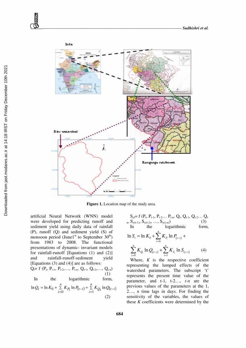
The study was conducted at Bino Watershed
under River Ramganga, a major tributary of
the River Ganga, which originates in the outer
Himalayas of Uttarakhand and drains into
River Bino. It is situated at 79° 6′ 14.4″ to 79
°
17′ 16.8″ E longitude and 29° 47′ 6″ to 30
° 02′
9.6″ N latitude in Almora and Pauri Garhwal
districts (Figure 1) having geographical area of
296.75 km2. Climate of the watershed varies
from Himalayan sub-tropical to sub-temperate
with mean annual maximum and minimum air
temperature of 30 and 18°C, respectively, and
mean annual rainfall of 931.3 mm. The daily
mean temperature remains high during months
of May and June, and minimum in December
and January. The daily rainfall in the
watershed was measured by non-recording
rain gauge at four raingauge stations viz.
Bungidhar, Jaurasi, Tamadhaun and Kedar,
runoff at the outlet by stage level recorder, and
sediment yield (suspended) were collected
from Divisional Forest Office, Ranikhet,
Uttarakhand. Weighted average values of daily
rainfall for the watershed were estimated by
Thiessen polygon method using ArcGIS 9.3
software. The runoff and sediment yield
collected have been reported in hectare-meter
(ham). Further, runoff was converted into
millimetre (mm) by dividing with the area of
the watershed and sediment load into kg sec-1
by multiplying with bulk density of silt as 1.4
gm cm-3.
Model Development
Three models, namely, Non-Linear
Dynamic model (NLD), Artificial Neural
Network (ANN) model, and Wavelet
Dow
nloa
ded
from
jast
.mod
ares
.ac.
ir at
14:
18 IR
ST
on
Frid
ay D
ecem
ber
10th
202
1
_____________________________________________________________________ Sudhishri et al.
684
Figure 1. Location map of the study area.
artificial Neural Network (WNN) model
were developed for predicting runoff and
sediment yield using daily data of rainfall
(P), runoff (Q) and sediment yield (S) of
monsoon period (June1st to September 30
th)
from 1983 to 2008. The functional
presentations of dynamic- invariant models
for rainfall-runoff [Equations (1) and (2)]
and rainfall-runoff-sediment yield
[Equations (3) and (4)] are as follows:
Qt= f (Pt, Pt-1, Pt-2,…, Pt-n. Qt-1, Qt-2,…, Qt-n)
(1)
In the logarithmic form,
( ) ( )∑
=
∑
=−− ++=
n
i
n
iitiQitiPt QKPKKQ
0 10 lnlnlnln
(2)
Syt= f (Pt, Pt-1, Pt-2… Pt-n. Qt, Qt-1, Qt-2… Qt-
n, Sy(t-1), Sy(t-2), …, Sy(t-n)) (3)
In the logarithmic form,
( )0
0
ln ln lni
n
t P t i
i
S K K P−
=
= + +∑
( ) ( )0 1
ln lni i
n n
Q St i t i
i i
K Q K S− −
= =
+∑ ∑ (4)
Where, K is the respective coefficient
representing the lumped effects of the
watershed parameters. The subscript ‘t’
represents the present time value of the
parameter, and t-1, t-2…, t-n are the
previous values of the parameters at the 1,
2…, n time lags in days. For finding the
sensitivity of the variables, the values of
these K coefficients were determined by the
Dow
nloa
ded
from
jast
.mod
ares
.ac.
ir at
14:
18 IR
ST
on
Frid
ay D
ecem
ber
10th
202
1
Simulating Runoff and Sediment Yield __________________________________________
685
multiple step-wise regression analysis and
variables found significant at 5% level were
only retained in the model. Any model
development means it should be used by the
end-users. In India particularly, most of the
watershed managers are Departmental
organizations. The employees are not well
versed with modern tools which needs skill.
But, non-linear dynamic models can be run
by simply using statistical software SPSS
and/or also excel sheet. Therefore, in this
study, a greater emphasis was given to
simple non-linear dynamic method. For
ANN and WNN, the predictor variables
were chosen by taking different
combinations of number of input parameters
equal or less than the maximum number of
model parameters determined through step-
wise regression tried in non-linear dynamic
model. Then, the two models were
compared with non-linear dynamic model
for both rainfall-runoff and rainfall-runoff-
sediment processes to get a better option.
An ANN is an information-processing
system composed of many nonlinear and
densely inter-connected processing elements
or neurons. The main function of the ANN
paradigms is to map a set of inputs to a set
of outputs. Sigmoid function is the most
commonly used non-linear activation
function in ANN. In the present study,
multilayer feed-forward networks which
are made up of multiple layers of neurons
with supervised learning using Back-
Propagation (BP) were used due to its
simplicity and effectiveness. The Haar-A-
Trous wavelet transform based Multi-
Resolution Analysis (MRA), which helps in
an efficient modeling of hydrological
processes, was used in this study
(Maheswaran and Khosa, 2012). It provides
a convincing and computationally very
straightforward solution while, at the same
time, avoiding the troublesome boundary
effects (Rathinasamy and Khosa, 2012);
Murtagh et al., 2004) and Wang and Ding,
2003). Wavelet transform was used to
decompose the rainfall and runoff time
series at level 3 into four sub-series (one
approximation and three details). This
appropriate decomposition level was
determined using the formula:
L= int (log(N)) (5)
Where, L indicates decomposition level
and N refers to the number of time series
data (Nourani et al., 2011; Adamowski and
Chan, 2011), which is 6,403 in this case
study. Due to proportional relationship
between amount of rainfall, runoff and
sediment load, they are supposed to have the
same seasonality levels. Therefore, all the
time series were decomposed at the same
level.
Input-Output Data Preparation and
Selection of Network Architecture
Daily rainfall, runoff, and sediment flow
data were used for training and testing of the
models. Analysis of daily surface runoff and
sediment yield revealed that past hydrologic
values of more than five days have no
significant effect on present day runoff or
sediment yield. Therefore, in this study a
maximum value of lag was taken as five and
multiple regression equations were
developed for runoff and sediment
prediction, respectively. The data in multiple
layer networks is divided into training,
validation, and testing (Liu et al., 2013) and
the ratio of partitioning taken as 60, 20, and
20%, respectively (Tiwari and Chatterjee,
2010). Therefore, 21 years’ (1983-2003)
daily records of the rainfall, runoff, and
sediment yield data were used for non-linear
dynamic model calibration and 5 years’
(2004-2008) data for testing. However, daily
data of 16 years (1983-1998), 5 years (1999-
2003), and 5 years (2004-2008) were used
for the training (calibration), validation, and
testing of ANN and WNN models,
respectively. For resolving daily data of
rainfall, runoff, and sediment yield, a
program developed in C++ language
(Tewari, 2007) and individual wavelet and
scale coefficients were calculated and used
for further analysis.
One of the most important attribute of a
layered neural network design is the
Dow
nloa
ded
from
jast
.mod
ares
.ac.
ir at
14:
18 IR
ST
on
Frid
ay D
ecem
ber
10th
202
1
_____________________________________________________________________ Sudhishri et al.
686
architecture. The size of the hidden layer(s)
is the most important consideration when
solving the actual problems using multilayer
feed-forward neural networks. However,
Shu and Ouarda (2007) recommended that
the number of hidden nodes should be less
than twice the number of input nodes. In this
study, the number of hidden nodes was
determined based on a trial-and-error
process that involved varying the number of
nodes from one to double the number of
input variables. There are several types of
ANNs but the major advantage of feed
forward back propagation ANN is that it is
less complex than other ANNs (Tiwari and
Chatterjee, 2010). Therefore, here sigmoid
feed forward activation function was used
for training ANN and WNN (Khalil et al.,
2011; Kisi, 2011). The Levenberg–
Marquardt methodology was used for
adjusting weights of the models due to its
being more powerful than conventional
gradient descent technique (Hagan and
Menhaj, 1994; Nakhaei and Nasr, 2012).
The training of ANN and WNN models is
similar to the calibration of conceptual
models. In the present study, input-output
pairs in the training and validation data sets
were applied to the network of a selected
architecture and training was performed.
Validation data set was used to apply an
early stopping approach related to epoch
size in order to avoid over training or over
fitting of the training data sets. Epoch is the
number of sets of training data and it is
recommended that the number of epochs
should be less than the number of input data
sets. Various networks of single and two
hidden layers were trained up to maximum
iterations or epochs of 2000, with different
combinations of hidden neurons and the best
suited network was selected based on the
minimum values of Root Mean Square Error
(RMSE), Akaike’s Information Criterion
(AIC) and maximum value of Coefficient of
determination (R2) (Agarwal et al., 2006).
Once the training process was satisfactorily
completed, the network was saved, the test
data sets were used for studying the best
performed model by the observed and
simulated values of runoff and sediment
yield. The normalized output values were
reconverted to give the predicted values of
runoff and sediment yield for comparison
with the corresponding observed values. The
analysis of ANN and WNN was performed
for predicting the runoff and sediment yield
by using NeuroSolutions 5.0 software. The
performance of the developed models was
assessed in terms of their R2, (RMSE)
(Agarwal, 2007), and model Efficiency (E)
(Nash and Sutcliffe, 1970; Rao et al., 2014).
In hydrological modeling, one of the major
concerns is estimating the flow or sediment
in extreme cases. Therefore, the models in
estimating the extreme values were
evaluated using Percent Error in Peak Flow
(PEPF) which measure only the magnitude
of peak flow and does not account for total
volume or timing of the peak (Asadi, 2013).
(6)
Where, Qo= Observed, Qs= Simulated
peak values.
RESULTS AND DISCUSSION
For rainfall-runoff modeling, based on the
step-wise regression, the Non-Linear
Dynamic (NLD) model with highest R2
(0.676) was built as follows:
( )
( ) ( ) ( )
1
1 2 3
ln 0.338 0.117 ln 0.044 ln
0.575ln 0.07955ln 0.124 ln
t t t
t t t
Q P P
Q Q Q
−
− − −
= + − +
+ +
(7)
Where, Q and P are in mm. It was
observed that, independent variables of
rainfall of present and previous day and
runoff of first, second, and third previous
days as the input to predict runoff on any
day was the best among the lag days tried.
As explained earlier, these five independent
variables are selected as the maximum
number of input to ANN and WNN models
(Tiwari and Chatterjee, 2010). Therefore,
different combinations of inputs viz. (i) Pt,
Pt-1, Qt-1, Qt-2, Qt-3 i.e., 5 inputs+1 output for
ANN and resolved 20 inputs+1 output for
WNN, (ii) Pt, Pt-1, Qt-1, Qt-2 i.e., 4 inputs+1
)(
)()(100
peakQo
peakQspeakQoPEPF
−=
Dow
nloa
ded
from
jast
.mod
ares
.ac.
ir at
14:
18 IR
ST
on
Frid
ay D
ecem
ber
10th
202
1
Simulating Runoff and Sediment Yield __________________________________________
687
output for ANN and resolved 16 inputs+1
output for WNN, and (iii) Pt, Qt-1, Qt-2 i.e., 3
inputs+1 output for ANN and 12 inputs+1
output for WNN were tried to get another
option of better combinations with minimum
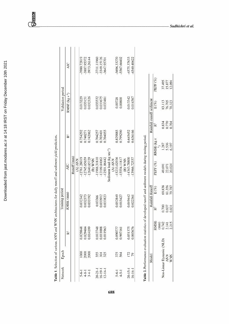
inputs. A few of the networks with single
layer having very low values of RMSE, AIC,
and higher value of R2 are shown in Table 1.
Inclusion of two hidden layers increased the
model running time significantly and also
had higher value of RMSE and low value of
R2, hence, not considered and the results are
not shown here. In ANN model, it was
observed that among 5 inputs, network
structure 5-6-1 (i.e. 5 inputs, 1 hidden layer
with 6 neurons and 1 output) with epochs of
1,000 was better as compared to the other
networks based on the performance criteria.
Similarly, among 4 inputs, networks, 4-8-1
and among 3 input, 3-4-1 networks with
epochs of 2000 were better having higher R2
and minimum RMSE and AIC. Out of these
ANN network structures; 5-6-1 network
structure was selected as the best performing
ANN model for prediction of daily runoff.
However, in case of WNN model, on the
basis of overall performance of the
attempted network structures, 20-21-1, 16-
19-1 and 12-14-1 were found to be
performing better at epochs of 355, 304 and
325, respectively. From these better
performing network structures, the 20-21-1
was finally selected as the best WNN model
with higher R2 and minimum RMSE and AIC
during training and testing periods at epoch
355 (Table 1).
For rainfall-runoff-sediment modeling,
the NLD model with highest R2 (0.872) was
built as:
( ) ( ) ( )1 2 1
ln 0.427 0.056ln 0.949ln
0.420ln 0.231ln 0.824ln
t t t
t t t
S P Q
Q Q S− − −
= − + + −
− +
(8)
Where, Q and P are in mm and S in kg s-1
.
In the development of ANN and WNN
models for sediment prediction, the input
status was kept the same as in the above
dynamic sediment model. As explained
earlier, various inputs parameters (i) Pt, Qt,
Qt-1, Qt-2, St-1 i.e., 5 inputs and 1 output for
ANN and resolved 20 inputs and 1 output
for WNN, (ii) Pt, Qt, Qt-1, St-1 i.e., 4 inputs
and 1 output for ANN and resolved 16
inputs and 1 output for WNN were used for
prediction of sediment load. Different
combinations of input and hidden layer
neurons were tried for developing the model
after selection of the best network
architecture. On the basis of overall
performance of the attempted network
structures, 5-6-1 and 4-5-1 network
structures with epochs 375 and 564,
respectively, were found to be performing
better. From these better performing
network structures, the 5-6-1 network
structure was finally selected as the best
ANN model having maximum R2 and
minimum RMSE and AIC (Table 1). In case
of WNN, among 20 inputs, the maximum
R2, minimum RMSE and AIC were observed
in 20-15-1 with epochs of 172 during both
training and validation period, whereas
among 16 inputs, the maximum R2,
minimum RMSE and AIC were observed in
16-15-1 during training, and higher R2 and
minimum RMSE in 16-14-1 were observed
at epochs of 79 during validation period.
Therefore, 16-14-1 was selected among 16
inputs. After comparison with the maximum
R2, minimum RMSE and AIC during both
training and validation periods, 20-15-1
network was found to be better.
All R2 and model Efficiency (%E) from
the ANN and WNN for runoff prediction
during testing period were much higher than
those from the NLD. Whereas, RMSE value
(1.287) from the NLD model during this
testing period was much lower than those for
the ANN and WNN, and the respective R2
(0.834) and E (83.113%) values were higher
in case of sediment yield prediction (Table
2). A visual assessment of the predicted and
observed runoff (Figure 2) shows that the
ANN predicted runoff had the best fit,
followed by WNN, and that the NLD fit was
the worst. Figure 3 shows the scatter plot
between the observed and predicted values
of NLD, ANN and WNN for sediment yield
and shows that the prediction of daily
Dow
nloa
ded
from
jast
.mod
ares
.ac.
ir at
14:
18 IR
ST
on
Frid
ay D
ecem
ber
10th
202
1
_____________________________________________________________________ Sudhishri et al.
688
Dow
nloa
ded
from
jast
.mod
ares
.ac.
ir at
14:
18 IR
ST
on
Frid
ay D
ecem
ber
10th
202
1
Simulating Runoff and Sediment Yield __________________________________________
689
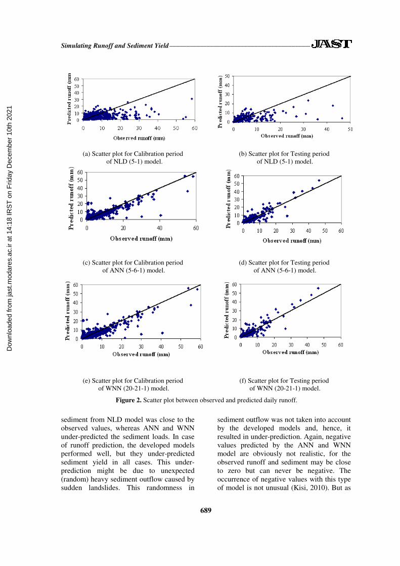
(a) Scatter plot for Calibration period
of NLD (5-1) model.
(b) Scatter plot for Testing period
of NLD (5-1) model.
(c) Scatter plot for Calibration period
of ANN (5-6-1) model.
(d) Scatter plot for Testing period
of ANN (5-6-1) model.
(e) Scatter plot for Calibration period
of WNN (20-21-1) model.
(f) Scatter plot for Testing period
of WNN (20-21-1) model.
Figure 2. Scatter plot between observed and predicted daily runoff.
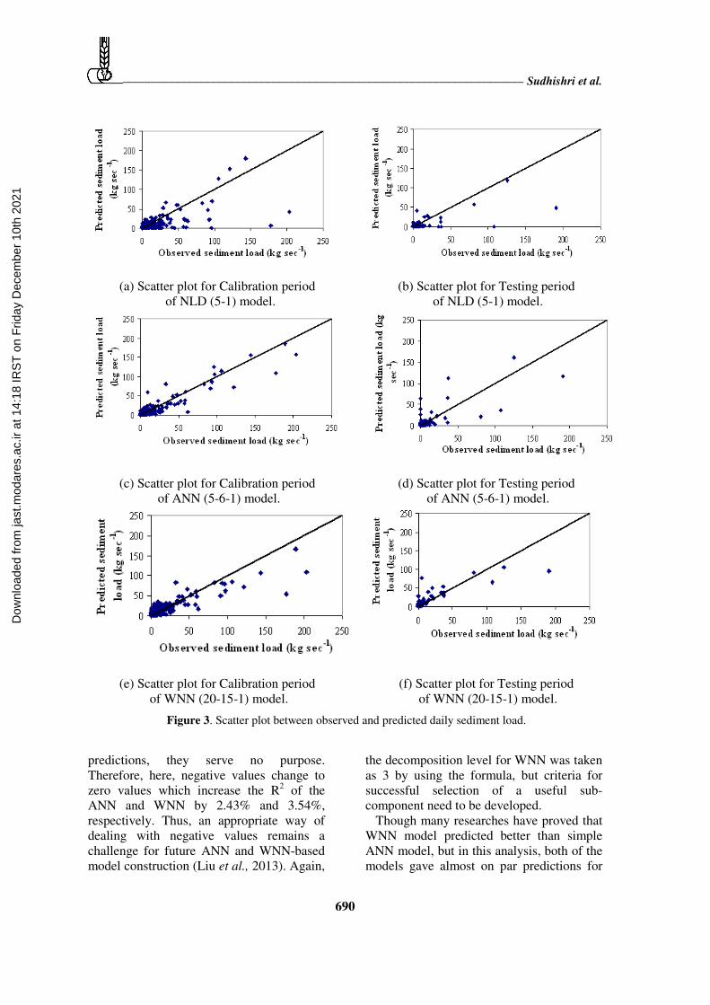
sediment from NLD model was close to the
observed values, whereas ANN and WNN
under-predicted the sediment loads. In case
of runoff prediction, the developed models
performed well, but they under-predicted
sediment yield in all cases. This under-
prediction might be due to unexpected
(random) heavy sediment outflow caused by
sudden landslides. This randomness in
sediment outflow was not taken into account
by the developed models and, hence, it
resulted in under-prediction. Again, negative
values predicted by the ANN and WNN
model are obviously not realistic, for the
observed runoff and sediment may be close
to zero but can never be negative. The
occurrence of negative values with this type
of model is not unusual (Kisi, 2010). But as
Dow
nloa
ded
from
jast
.mod
ares
.ac.
ir at
14:
18 IR
ST
on
Frid
ay D
ecem
ber
10th
202
1
_____________________________________________________________________ Sudhishri et al.
690
(a) Scatter plot for Calibration period
of NLD (5-1) model.
(b) Scatter plot for Testing period
of NLD (5-1) model.
(c) Scatter plot for Calibration period
of ANN (5-6-1) model.
(d) Scatter plot for Testing period
of ANN (5-6-1) model.
(e) Scatter plot for Calibration period
of WNN (20-15-1) model.
(f) Scatter plot for Testing period
of WNN (20-15-1) model.
Figure 3. Scatter plot between observed and predicted daily sediment load.
predictions, they serve no purpose.
Therefore, here, negative values change to
zero values which increase the R2 of the
ANN and WNN by 2.43% and 3.54%,
respectively. Thus, an appropriate way of
dealing with negative values remains a
challenge for future ANN and WNN-based
model construction (Liu et al., 2013). Again,
the decomposition level for WNN was taken
as 3 by using the formula, but criteria for
successful selection of a useful sub-
component need to be developed.
Though many researches have proved that
WNN model predicted better than simple
ANN model, but in this analysis, both of the
models gave almost on par predictions for
Dow
nloa
ded
from
jast
.mod
ares
.ac.
ir at
14:
18 IR
ST
on
Frid
ay D
ecem
ber
10th
202
1
Simulating Runoff and Sediment Yield __________________________________________
691
runoff and sediment yield. This may be due
to the fact that large mountainous catchment
runoff and the sediment yield generated are
discontinuous for so many days and again
the lag values were fixed for both of the
models, taking into account the resulting lag
values through simple and easily computable
non-linear dynamic model by simple
software or excel sheet. Peak value is a key
point in the time series modeling. The
results reported here are based on the whole
time series data. Since the WNN model is a
multi-scaled and seasonal model and ANN
is autoregressive model, it is expected that
WNN has a better ability to capture peak
values. Therefore, analysis was done for
peak flows. PEPF values of 20.024 and
12.094 were observed for runoff and
sediment yield, respectively, which are less
than that of ANN and NLD (Table 2). This
indicates the greater capturing power of
WNN for simulating extreme flows (Rao et
al., 2014; Tiwari and Chatterjee, 2010). This
under-prediction may be due to unexpected
(random) heavy sediment outflow due to
sudden landslides. This randomness in
sediment outflow is not taken into account
by the developed models and, hence, it
results in under-prediction.
CONCLUSIONS
In this work, performance of feed forward
ANN and Wavelet based ANN (WNN) has
been reported, taking the input parameters
obtained through step-wise regression done
for Non-Linear Dynamic (NLD) model for
predicting daily runoff and sediment yield
considering the memory system of a
Himalayan Mountainous Watershed in
Uttarakhand, India. Twenty-six years’ of
daily rainfall, runoff and sediment yield data
of monsoon period of Bino Watershed under
Ramganga catchment were used for the
analysis. The performance of a developed
model was assessed in terms of its
coefficient of determination, root mean
square error, and model efficiency. The
results revealed superior performance of
the ANN and WNN models in comparison
to the NLD model in case of rainfall-
runoff process, whereas NLD model
performed well compared to ANN and
WNN models in case of rainfall-runoff-
sediment process. The comparison
revealed that, for runoff modeling, ANN
and WNN performed at par, whereas for
sediment yield prediction, NLD model
performed well. However, the models
under-predicted sediment yield. This could
be due to not considering randomness in
values resulting from sudden landslides and
flash floods in Himalayan Watersheds.
Again, criteria for successful selection of a
useful sub-component in WNN need to be
developed. Further, the WNN performance
was evaluated for peak flows, which
revealed that WNN performed better
compared to ANN and NLD. Therefore,
this study suggests that, in mountainous
watershed, due to more dynamic nature of
hydrologic events, it is very difficult to
generalize that WNN is better than ANN
and/or non-linear models. This indicates the
capturing power of WNN model for
simulation for extreme flows in mountainous
watershed compared to whole time series
data.
REFERENCES
1. Adamowski, J. F. 2008. Development of a
Short-term River Flood Forecasting Method
for Snowmelt Driven Floods Based on
Wavelet and Cross Wavelet Analysis. J.
Hydrol., 353: 247-266.
2. Adamowski, J. and Sun, K. 2010.
Development of a Coupled Wavelet
Transform and Neural Network Method for
Flow Forecasting of Non-perennial Rivers in
Semi-arid Watersheds. J. Hydrol., 390(1-2):
85-91.
3. Adamowski, J. and Chan, H. F. 2011. A
Wavelet Neural Network Conjunction
Model for Groundwater Level Forecasting.
J. Hydrol., 407: 28–40.
4. Agarwal, A., Mishra, S. K., Ram, S. and
Singh, J. K. 2006. Simulation of Runoff and
Sediment Yield Using Artificial Neural
Networks. Biosyst. Eng., 94(4): 597-613.
Dow
nloa
ded
from
jast
.mod
ares
.ac.
ir at
14:
18 IR
ST
on
Frid
ay D
ecem
ber
10th
202
1
_____________________________________________________________________ Sudhishri et al.
692
5. Agarwal, B. L. 2007. Basic Statistics. New
Age International (P) Ltd., Publishers, New
Delhi, India,763 PP.
6. Agarwal, R. K and Singh, J. K. 2003.
Application of a Genetic Algorithm in the
Development and Optimization of a Non-
linear Dynamic Runoff Model. Biosyst.
Eng., 86(1): 87-95.
7. Asadi, A. 2013. The Comparison of Lumped
and Distributed Models for Estimating Flood
Hydrograph (Study Area: Kabkian Basin). J.
Electron.Commun. Eng. Res., 1(2): 7-13.
8. Cannas, B., Fanni, A., Sias, G., Tronci, S.
and Zedda, M. K. 2005. River Flow
Forecasting Using Neural Networks and
Wavelet Analysis. Geophys. Res. Abstr.
7(08651). Ref-ID: 1607-7962/gra/EGU05-
A-08651 © European Geosciences Union
2005.
9. Coulibaly, P., Anctil, F. and Bobee, B. 2000.
Daily Reservoir Inflow Forecasting Using
Artificial Neural Networks with Stopped
Training Approach. J. Hydrol., 230: 244-
257.
10. Hagan, M. T. and Menhaj, M. 1994.
Training Feed Forward Networks with the
Marquardt Algorithm. IEEE Trans. Neural
Network., 5(6): 989–993.
doi:10.1109/72.329697.
11. Khalil, B., Ouarda,T. B. M. J. and St-
Hilaire, A. 2011. Estimation of Water
Quality Characteristics at Ungauged Sites
Using Artificial Neural Networks and
Canonical Correlation Analysis. J. Hydrol.,
405: 277-287.
12. Kim, T. W. and Valdes, J. B. 2003. Non-
linear Model for Drought Forecasting Based
on a Conjunction of Wavelet Transforms
and Neural Networks. J. Hydrol. Eng., 6:
319-328.
13. Kisi, O. 2011. Wavelet Regression Model as
an Alternative to Neural Network for River
Stage Forecasting. Water Resour. Manage.,
25:579-600.
14. Kisi, O. 2010. Daily Suspended Sediment
Estimation Using Neuro-wavelet Models.
International J. Earth Sciences. 99:1471-
1482.
15. Kumar, A. 1993. Dynamic Nodels for Daily
Rainfall-runoff-sediment Yield for Sub-
catchment of Ramganga River. PhD. Thesis,
Department of Soil and Water Conservation
Engineering, G. B. Pant University of
Agriculture and Technology, Pantnagar,
India.
16. Liu, Q. J., Shi, Z. H., Fang, N. F., Zhu, H. D.
and Ai, L. 2013. Modeling the Daily
Suspended Sediment Concentration in a
Hyperconcentrated River on the Loess
Plateu, China Using Wavelet-ANN
Approach. Geomorpol., 186: 181-190.
17. Maheswaran R. and Khosa R. 2012.
Comparative Study of Different Wavelets
for Hydrologic Forecasting. Comput.
Geosci. 46:284-295.
18. Murtagh, F., Starck, J. L. and Renaud, O.
2004. On Neuro-wavelet Modeling. Decis.
Support Syst., 37: 475-484.
19. Muttil, N. and Chau, K.W. 2006. Neural
Network and Genetic Programming for
Modeling Coastal Algal Blooms. Int. J.
Environ. Pollut., 28(3-4): 223-238.
20. Nakhaei, M. and Nasr, A. S. 2012. A
Combined Wavelet-artificial Neural
Network Model and Its Application to the
Prediction of Groundwater Level
Fluctuations. JGeope, 2(2): 77-91.
21. Nash, J. E. and Shutcliff, J. V. 1970. River
Flow Forecasting through Conceptual
Models-I. J. Hydrol., 10: 282-290.
22. Nourani, V., Kisi, O. and Komasi, M. 2011.
Two Hybrid Artificial Intelligence
Approaches for Modeling Rainfall-runoff
Process. J. Hydrol., 402(1-2): 41-59.
23. Partal, T. and Kisi, O. 2007. Wavelet and
Neuro Fuzzy Conjunction Model for
Precipitation Forecasting. J. Hydrol.,
342:199-212.
24. Partal, T. and Cigizoglu, H. K. 2008.
Estimation and Forecasting of Daily
Suspended Sediment Data Using Wavelet-
neural Networks. J. Hydrol., 358(3–4):317–
331.
25. Rao, Y. R. S., Krisha, B. and Venkatesh, B.
2014. Wavelet Based Neural Networks for
Daily Stream Flow Forecasting. Int. J.
Emerg. Technol. Adv. Eng., 4(1): 307-317.
26. Rathinasamy, M. and Khosa, R. 2012.
Multiscale Nonlinear Model for Monthly
Streamflow Forecasting: A Wavelet-based
Approach. J. Hydroinform., 14(2): 424-442.
27. Remesan, R., Shamim, M. A., Han, D. and
Mathew, J. 2009. Runoff Prediction Using
an Integrated Hybrid Modelling Scheme. J.
Hydrol., 372(1-4): 48-60.
28. Sachan, A. 2008. Suspended Sediment Load
Prediction Using Wavelet Neural Network
Model. MTech. Thesis. Department of
SWCE, GBPUAT, Pantnagar (UK), India,
152 PP.
Dow
nloa
ded
from
jast
.mod
ares
.ac.
ir at
14:
18 IR
ST
on
Frid
ay D
ecem
ber
10th
202
1
Simulating Runoff and Sediment Yield __________________________________________
693
29. Shu, C. and Ouarda, T. B. M. J. 2007. Flood
Frequency Analysis at Ungauged Sites
Using Artificial Neural Networks in
Canonical Correlation Analysis
Physiographic Space. Water Resour. Res.,
43: W07438. doi:10.1029/2006WR005142.
30. Sivakumar, B., Jayawardena, A. W. and
Fernando, T. M. K. G. 2002. River Flow
Forecasting: Use of Phase-space
Reconstruction and Artificial Neural
Networks Approaches. J. Hydrol., 265: 225-
245.
31. Taormina, R., Chau, K. W. and Sethi, R.
2012. Artificial Neural Network Simulation
of Hourly Groundwater Levels in a Coastal
Aquifer System of the Venice Lagoon. Eng.
Appl. Artif. Intel., 25(8): 1670-1676.
32. Tewari, S. 2007. Haar-A Trous Wavelet
Transform based Mulit-resolution Grey
Model for Runoff Prediction. MTech.
Thesis. Department of SWCE, GBPUAT,
Pantnagar (UK), 74 PP.
33. Tiwari, M. K. and Chatterjee, C. 2010.
Development of an Accurate and Reliable
Hourly Flood Forecasting Model Using
Wavelet-Bootstrap-ANN (WBANN) Hybrid
Approach. J. Hydrol., 394(3-4): 458-470.
34. Wang, W. and Ding, J. 2003. Wavelet
Network Model and Its Application to the
Prediction of Hydrology. Nat. Sci., 1(1): 67-
71.
35. Wu, C. L., Chau, K. W. and Li, Y. S. 2009.
Predicting Monthly Streamflow Using Data-
driven Models Coupled with Data-
preprocessing Techniques. Water Resour.
Res., 45: W08432.
doi:10.1029/2007WR006737.
ارزيابي تطبيقي مدل هاي شبكه عصبي و مبتني بررگرسيون براي شبيه سازي رواناب
و توليد رسوب در يك حوضه آبريز بيرون از هيماليا
ج. ك. سينك و س. سودهيشري، ا. كومار،
چكيده
پيچيدگي فرايند هيدرولوژيكي در پيش بيني رواناب و توليد رسوب در حوضه هاي كوهستاني وسيع،
توليد رسوب همچنان به عنوان يك چالش باقي مانده است.در پژوهش حاضر، يك -انابرو-بارندگي
) براي پيش بيني رواناب و simple non-linear dynamic, NLDمدل ساده وغير خطي پويا (
- توليد رسوب روزانه و با در نظر گرفتن تاريخچه بارندگي و رواناب حوضه آبريز و رابطه بارندگي
) و ANNسوب به كاررفت. نتايج به دست آمده با دو مدل شبكه عصبي مصنوعي (رواناب و توليد ر
ANN) موجكwavelet based ANN, WNN كه رايج هستند مقايسه شدند و اين كار با (
) maximum input parameters of valuesاستفاده از مقدار حد اكثر پارامترهاي نهاده اي (
) براي بارندگي، رواناب، و توليد رسوب به دست آمده از time memoryمربوط به حافظه زماني (
feedاز نوع ANNو از طريق رگرسيون گام به گام انجام شد.مدل هاي NDLمدل توسعه يافته
forward ) با الگوريتم تكثير پسينback propagation مورد استفاده قرار گرفت. در اين پژوهش (
درايالت آتاراخند Bino ساله حوضه 26وليد رسوب يك دوره از آمار روزانه بارندگي، رواناب، و ت
استفاده شد. براي ارزيابي عملكرد مدل ازضريب تبيين، ريشه ميانگين مربعات خطا و كارآيي مدل
Dow
nloa
ded
from
jast
.mod
ares
.ac.
ir at
14:
18 IR
ST
on
Frid
ay D
ecem
ber
10th
202
1

_____________________________________________________________________ Sudhishri et al.
694
و ANNرواناب -استفاده شد. نتايج به دست آمده حاكي از عملكرد بهتر براي مدل هاي بارندگي
WNN در مقايسه باNLD كه در حالتي كه تمام داده هاي سري زماني در نظر گرفته شد بود، هرچند
داشت. دليل اين كه WNNو ANNكارآيي بيشتري از NLDتوليد رسوب -رواناب-مدل بارندگي
ا كم پيش بيني مي كردند وقوع ناگهاني زمين لغزه و سيل هاي شديد در همه مدل ها توليد رسوب ر
بود، كاربرد NLDو ANNبهتر از WNNحوضه هاي هيماليا بود. نتايج پژوهش نشان داد كه هرچند
اين مدل را براي همه حوضه هاي كوهستاني نمي توان تعميم داد. مجددا ياد آوري مي شود كه ضوابط
مي بايست فراهم آيد. همچنين، اين پژوهش چنين اشاره دارد WNNجزء در -انتخاب موفق يك زير
) توانايي بيشتري براي peak flowبا كمترين درصد اشتباه در مورد جريان اوج ( WNNكه مدل
شبيه سازي جريانات فوق العاده را دارد.
Dow
nloa
ded
from
jast
.mod
ares
.ac.
ir at
14:
18 IR
ST
on
Frid
ay D
ecem
ber
10th
202
1
Recommended