Discussion Paper No. 06-007
Combining Top-Down and Bottom-up in Energy Policy Analysis:
A Decomposition Approach
Christoph Böhringer and Thomas F. Rutherford

Discussion Paper No. 06-007
Combining Top-Down and Bottom-up in Energy Policy Analysis:
A Decomposition Approach
Christoph Böhringer and Thomas F. Rutherford
Die Discussion Papers dienen einer möglichst schnellen Verbreitung von neueren Forschungsarbeiten des ZEW. Die Beiträge liegen in alleiniger Verantwortung
der Autoren und stellen nicht notwendigerweise die Meinung des ZEW dar.
Discussion Papers are intended to make results of ZEW research promptly available to other economists in order to encourage discussion and suggestions for revisions. The authors are solely
responsible for the contents which do not necessarily represent the opinion of the ZEW.
Download this ZEW Discussion Paper from our ftp server:
ftp://ftp.zew.de/pub/zew-docs/dp/dp06007.pdf
Nontechnical Summary The combination of bottom-up and top-down approaches constitutes a long-standing challenge in applied
energy policy analysis. The terms ``top-down'' and ``bottom-up'' are shorthand for aggregate and
disaggregated models. Top-down models examine the broader economy and incorporate feedback effects
between different markets triggered by policy-induced changes in relative prices and incomes. They
typically do not feature technological details of energy production or conversion. Energy sectors – like
other non-energy sectors – are mostly represented in an aggregate way by means of smooth production
functions which capture substitution (transformation) possibilities via substitution (transformation)
elasticities. As a consequence, conventional top-down models cannot readily incorporate different
assumptions about how discrete energy technologies and costs will evolve in the future; top-down models
may also violate fundamental physical restrictions such as the conservation of matter and energy. In
contrast, bottom-up models -- usually cast as mathematical programming problems – describe current and
prospective technologies in detail. They are therefore well suited to the analysis of specific changes in
technology or command-and-control policies such as efficiency standards. A common shortcoming of the
bottom-up analysis is that it fails to account for price distortions, economy-wide interactions and income
effects.
The formulation of economic equilibrium conditions as mixed complementarity problem (MCP) provides
a unifying framework for combining technological details of bottom-up models and economic richness of
top-down models. However, dimensionality may impose significant limitations on the practical
application of the integrated MCP framework, particularly when the underlying programming formulation
of the energy system includes both upper and lower bounds on many decision variables.
In this paper, we present a decomposition approach that combines different mathematical formats –
mixed complementarity and mathematical programming – thereby taking advantage of efficient and
robust solution algorithms for each format: We use complementarity methods to solve the top-down
economic equilibrium model and quadratic programming to solve the underlying bottom-up energy
supply model. Our decomposition technique overcomes dimensionality restrictions of the integrated MCP
framework and can be readily applied to the combination of large-scale top-down and bottom-up models
for comprehensive energy policy analysis.
Combining Top-Down and Bottom-Up in Energy Policy Analysis:
A Decomposition Approach
Christoph Bohringer
Centre for European Economic Research (ZEW), Mannheim, Germany
Department of Economics, University of Heidelberg, Germany
and
Thomas F. Rutherford
Ann Arbor, MI, U.S.A.
Abstract
The formulation of market equilibrium problems as mixed complementarity problems (MCP)
permits integration of bottom-up programming models of the energy system into top-down
general equilibrium models of the overall economy. Despite the coherence and logical appeal
of the integrated MCP approach, implementation cost and dimensionality both impose lim-
itations on its practical application. A complementarity representation involves both primal
and dual relationships, often doubling the number of equations and the scope for error. When
an underlying optimization model of the energy system includes upper and lower bounds on
many decision variables the MCP formulation may suffer in robustness and efficiency. While
bounds can be included in the MCP framework, the treatment of associated income effects
is awkward.
We present a decomposition of the integrated MCP formulation that permits a convenient
combination of top-down general equilibrium models and bottom-up energy system models
for energy policy analysis. We advocate the use of complementarity methods to solve the
top-down economic equilibrium model and quadratic programming to solve the underlying
bottom-up energy supply model. A simple iterative procedure reconciles the equilibrium
prices and quantities between both models. We illustrate this approach using a simple
stylized model.
JEL classification: C61, C68, D58, Q43
Keywords: Mathematical Programming, Mixed Complementarity, Top-Down/Bottom-Up
1 Introduction
Top-down and bottom-up are the two modeling paradigms to represent interactions between
the energy system and the economy (International Panel on Climate Change (IPCC) [1996]).
The terms “top-down” and “bottom-up” are shorthand for aggregate and disaggregated
models. Models in the first category emphasize economy-wide, while those in the second
category feature sectoral and technological details. The dichotomy of energy-economy models
into top-down and bottom-up approaches is sometimes traced back to competing paradigms.
It should be noted, however, that differences are less of conceptual nature, i.e. due to
controversial theoretical underpinnings, but simply relate to the different levels of sectoral
and technological aggregation as well as to the scope of ceteris paribus assumptions.
Top-down models examine the broader economy and incorporate feedback effects between
different markets triggered by policy-induced changes in relative prices and incomes. They
typically do not feature technological details of energy production or conversion. Energy
sectors – like other non-energy sectors – are mostly represented in an aggregate way by means
of smooth production functions which capture substitution (transformation) possibilities via
substitution (transformation) elasticities. As a consequence, conventional top-down models
cannot readily incorporate different assumptions about how discrete energy technologies
and costs will evolve in the future; top-down models may also violate fundamental physical
restrictions such as the conservation of matter and energy.
In contrast, bottom-up models – usually cast as mathematical programming problems –
describe current and prospective technologies in detail. They are therefore well suited to the
analysis of specific changes in technology or command-and-control policies such as efficiency
standards. A common shortcoming of the bottom-up analysis is that it fails to account for
price distortions, economy-wide interactions and income effects (e.g. revenue recyling effects
of energy taxes).
There are various hybrid modeling efforts that aim at combining the technological ex-
plicitness of bottom-up models with the economic richness of top-down models. These ef-
forts can be broadly classified into two approaches. The first approach attempts to couple
existing large-scale bottom-up and top-down models (e.g. Hudson and Jorgenson [1974],
Bergmann [1990]). Due to the heterogeneity in complexity and accounting methods across
the sub-models such a “soft-link” approach may face substantial problems in achieving over-
all consistency and convergence of iterative solution algorithms.1 The second approach puts
strong emphasis on overall economic consistency and therefore makes use of a single inte-
grated modeling framework in order to “hard-link” bottom-up and top-down features. Such
an integrated framework is provided by the specification of market equilibrium models as
mixed complementarity problems (MCP – see Cottle and Pang [1992], Rutherford [1995]).
1Manne and Rutherford [1994] employ iterative methods to incorporate general equilibrium effects within the
context of technology-oriented bottom-up models.
1
The explicit representation of weak inequalities and complementarity between decision
variables and market equilibrium conditions in the MCP formulation permits the modeler
to capture both technological details and economic richness in a single mathematical format
(Bohringer [1998]). More recently, the availability of robust large-scale solvers for MCP
problems (Dirkse and Ferris [1995]) has promoted the implementation and application of
hybrid energy-economy models in the MCP format to concrete energy regulation policies
(e.g. Bohringer et al. [2003] or Frei et al. [2003]).
Despite the coherence and logical appeal of the integrated MCP approach, algebraic com-
plexity and dimensionality impose significant limitations on its practical application, when
the optimization problem describing the energy system includes upper and lower bounds on
many decision variables. Bounds may also be incorporated in the MCP framework but the
representation of associated income effects becomes rather problematic.
In this paper, we propose a decomposition technique to overcome such dimensionality
restrictions. We describe how an integrated MCP model can be decomposed and solved
iteratively: Complementarity methods are used to solve the top-down economic equilibrium
model and quadratic programming is applied to solve the underlying bottom-up energy
(supply) model. We present a worked example which illustrates the usefulness of the energy-
sector decomposition, both in terms of efficiency of computation and transparency of model
formulation. Convergence of our iterative (Jacobi) algorithm requires that the decomposed
energy sector be small relative to the rest of the economy. In this setting, a Marshallian
demand approximation in the energy sector model provides a precise local representation of
the general equilibrium demand so that overall convergence occurs rapidly.2
The remainder of this paper is organized as follows. In section 2, we extend the top-down
representation of economic market equilibria as a mixed complementarity problem by an
explicit bottom-up linear programming sub-model of energy supply. In section 3, we lay out
how the integrated top-down / bottom-up MCP model can be decomposed. In section 4, we
provide an illustrative numerical example. In secton 5, we conclude.
2 Integrated Model Formulation
Market equilibrium features complementarity between upper and lower bounds on equi-
librium variables and the weak inequalities which characterize market equilibrium. The
complementarity features of market equilibria motivate the mathematical formulation of
market equilibrium problems as a mixed complementarity problem (MCP). The MCP ap-
proach provides a general mathematical format that covers weak inequalities, i.e. a mixture
2In applications in which the energy system turns out to be of sufficient significance that the decomposition is
costly or unreliable, our use of a complementarity formulation for the general equilibrium model permits selected
features of the energy sector to be computed simultaneously with the macro-economy; the remaining part of the
energy systen can then still be solved as a quadratic programming problem.
2
of equations and inequalities, and complementarity between variables and functional rela-
tionships. It includes a wide range of mathematical problems including systems of linear or
nonlinear equations or mathematical programs (Rutherford [1995]). The MCP formulation
relaxes the integrability constraints for equilibrium conditions which emerge as first-order
conditions from primal or dual optimization problems. This permits the direct representa-
tion of market inefficiencies such as distortionary taxes or spillovers that cannot be readily
studied in an optimization framework (Bohringer and Rutherford [2005]).
In our formulation of an integrated top-down / bottom-up model we consider a com-
petitive (Arrow-Debreu) economy with n commodities (including economic goods, energy
goods and primary factors) indexed by i, m production activities (sectors) indexed by j,
and h households (including government) indexed by k. We extend the MCP framework
suggested by Mathiesen [1985] by embedding an explicit linear-programming sub-model of
energy supply in the economy. The decision variables of the economy can be classified into
the following categories:
p denotes a non-negative n-vector in prices for all goods and factors,
y is a non-negative m-vector for activity levels of constant-returns-to-scale (CRTS) produc-
tion sectors,
M is a h-vector of consumer income levels,
e represents a non-negative n-vector of net energy system outputs (including, for example,
electricity, oil, coal, and natural gas supplies to residential, industrial, and commercial
customers), and
x denotes a non-negative n-vector of energy system inputs (including labor, capital, and
materials inputs).
As in Mathiesen’s model a competitive market equilibrium for this economy is represented
by a vector of activity levels, a non-negative vector of prices, and a non-negative vector of
incomes such that:
• No production activity makes a positive profit (zero-profit condition):3
−Πj(p) ≥ 0 (1)
in which Πj(p) denotes the unit profit function for CRTS production activity j, which
is calculated as the difference between unit revenue and unit cost (i.e., Πj(p) = rj(p)−cj(p)).
3We omit tax distortions from this exposition solely to economize on notation. An important and appealing
feature of the top-down general equilibrium framework is its ability to address the welfare consequences of energy
policy from a public finance perspective, i.e. accounting for initial tax distortions and public sector budget
constraints.
3
• Excess supply (supply minus demand) is non-negative for all goods and factors (market
clearance condition):
∑
j
∇Πj(p) yj +∑
k
ωk + e ≥∑
k
dk(p,Mk) + x (2)
in which ωk indicates the initial endowment vector for household k and d(k,Mk) is the
utility-maximizing demand vector for household k.
• Expenditure does not exceed income (budget constraint):
Mk = pT [ ωk + θk(e− x) ] (3)
in which θk represents the share of energy-sector rents that accrue to household k
(rents depend on household ownership of energy resources). The equations which de-
fine consumer income levels are conceptually distinct from the zero profit and market
clearing conditions in that there is no explicit complementarity at work in this part of
the model. The income variables are added to the equilibrium system solely as a means
of simplifying the expression of household demand.
Furthermore, we assume that the equilibrium levels of energy sector outputs and inputs
are consistent with profit-maximization, taking market prices as given:
• Energy sector supply and demand vectors are profit-maximizing choices subject to tech-
nical constraints. That is, e and x solve a linear programming model. For concreteness,
we will assume that this bottom-up model can be written as:
max pT (e− x) (4)
subject to
Ax + Bz ≥ Ce
e, x ≥ 0, ` ≤ z ≤ u
in which A,C ∈ RM×n, and B ∈ RM×N characterize technical constraints and z ∈ RN
denotes decision variables of the energy system.
In the integrated model formulation the linear program can be incorporated through the
associated Kuhn-Tucker conditions and solved simultaneously with the equilibrium condi-
tions (1)-(3):
CT π ≥ p, e ≥ 0, eT (CT π − p) = 0
p ≥ AT π, x ≥ 0, xT (p−AT π) = 0
Ax + Bz ≥ Ce, π ≥ 0, πT (Ax + Bz − Ce) = 0
` ≤ z ≤ u, λ, µ ≥ 0, λ(z − `) = 0, µ(u− z) = 0
λ + BT π = µ
4
The attribution of energy-sector rents to households can be made explicit by writing (3)
as:
Mk = pT ωk + Θk(µT u + λT `)
in which Θk ∈ Rh×N determines rents on energy-sector resources to households.
The integrated equilibrium for this hybrid top-down / bottom-up model then consists
of m + 3n + h + M + 3N equations as compared with the standard economic model of
dimension m + n + h and the original linear programming model with M constraints and
N + 2n variables.4 If computational complexity increases superlinearly with the problem
dimension, a decomposition approach can outperform a simultaneous solution algorithm,
provided that sufficiently few outer iterations are required to solve the decomposed model.
3 A Decomposition Strategy
The introduction of an energy-sector sub-model within the general equilibrium framework
poses computational challenges when the dimensionality of the energy sector – captured by
N + M in our abstract setting – is very large relative to the dimensionality of the standard
economic model given by n + m + h. While an integrated MCP formulation is attractive for
highly aggregated energy system representations, it has limited practicality for large-scale
systems with bounds on many variables due to the need to account for associated income
effects. The added dimensionality poses two problems. First, the enlarged system may
be more difficult to solve. Second, and more importantly in our view, the model is more
awkward to implement because of the larger number of variables and equations as well as
the complexity of explicit income constraints. Compactness of representation leads to fewer
potential sources of error and more rapid model development. Calendar time rather than
CPU time is the primary concern of the applied analyst.
In view of the challenges presented by the complementarity format we propose a decom-
position strategy for the integrated model in which the energy system bottom-up component
can be computed separately from the top-down economic general equilibrium sub-model.
The solution procedure involves iterative solution of the top-down general equilibrium model
given net supplies from the bottom-up energy sector sub-model followed by the solution of
the energy sector sub-model based on a locally calibrated set of demand functions for energy
sector outputs. When (e−x) and θ are given exogenously, the top-down general equilibrium
model can be solved as a complementarity problem of dimension m + n + h.
Suppose that the computed equilibrium prices are p (based on an initial guess for the
energy sector response e, x, and θ). The next step in a recursive solution procedure updates
the values of (e − x) and θ based on p. One might then consider a direct solution of the
4The linear programming model represents upper and lower bounds on decision variables through implicit
Kuhn-Tucker conditions, such that we can reduce the number of constraints by 2N as compared with the integrated
MCP formulation.
5
profit-maximizing linear program (4) which characterizes the choices of an individual firm.
However, this approach is quite likely to fail because the profit-maximizing linear program
does not take account of the response of market demand to changes in energy prices. Suppose
that these demand elasticities are given by ε.5 We can then write the demand for energy
good i as:
ei(p) = ei [1− εi(pi/pi − 1)]
where εi is the demand elasticity and ei and pi denote the observable reference quantities
and prices for the demand function calibration.
The calibrated inverse demand function is:
pi(e) = pi [1− (1− ei/ei)/εi]
and the integrated market demand function is:∫
pi(ei)dei = piei
[1− ei − 2ei
2εiei
],
Am aggregate (integrated) multicommodity energy systemn may then be solved as a
quadratic programming problem of the form:6
max pT (e− x)− 12
∑
i
piei
εiei(ei − 2ei) (5)
subject to the same constraints which appear in (4) in order to compute a partial market
equilibrium model for the energy sector based on linear demand functions locally calibrated
to the given macroeconomic equilibrium.
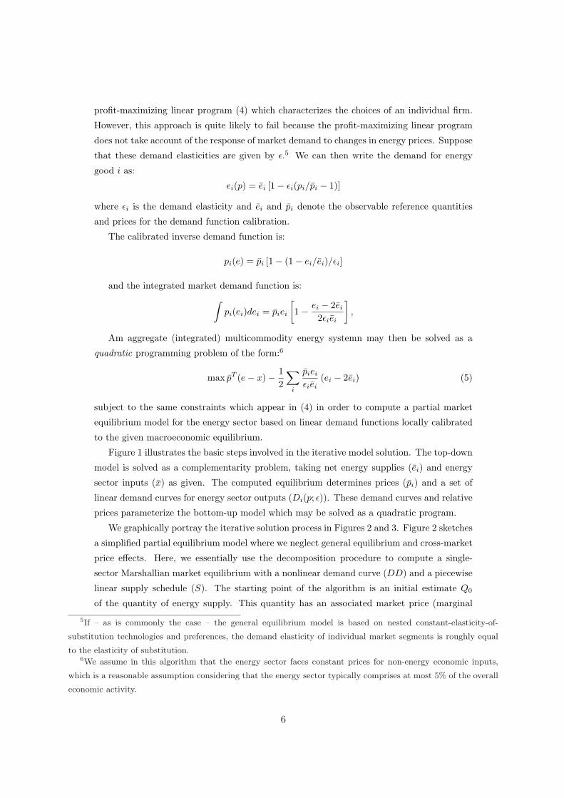
Figure 1 illustrates the basic steps involved in the iterative model solution. The top-down
model is solved as a complementarity problem, taking net energy supplies (ei) and energy
sector inputs (x) as given. The computed equilibrium determines prices (pi) and a set of
linear demand curves for energy sector outputs (Di(p; ε)). These demand curves and relative
prices parameterize the bottom-up model which may be solved as a quadratic program.
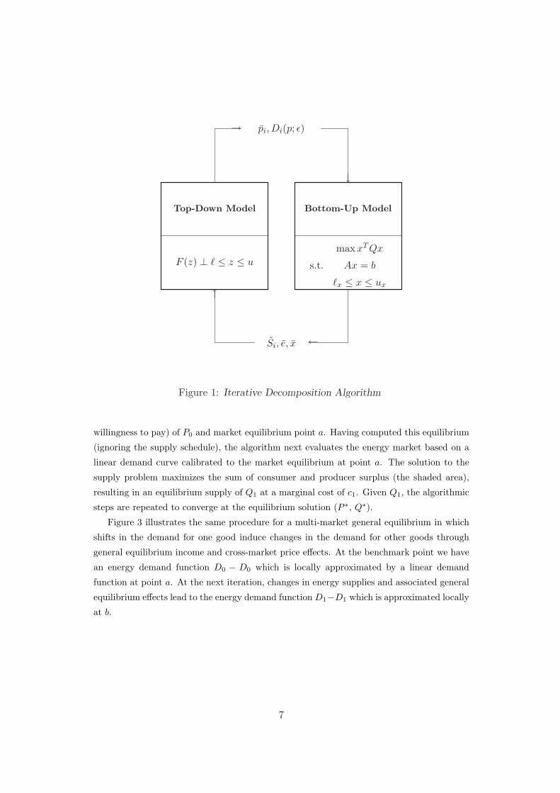
We graphically portray the iterative solution process in Figures 2 and 3. Figure 2 sketches
a simplified partial equilibrium model where we neglect general equilibrium and cross-market
price effects. Here, we essentially use the decomposition procedure to compute a single-
sector Marshallian market equilibrium with a nonlinear demand curve (DD) and a piecewise
linear supply schedule (S). The starting point of the algorithm is an initial estimate Q0
of the quantity of energy supply. This quantity has an associated market price (marginal
5If – as is commonly the case – the general equilibrium model is based on nested constant-elasticity-of-
substitution technologies and preferences, the demand elasticity of individual market segments is roughly equal
to the elasticity of substitution.6We assume in this algorithm that the energy sector faces constant prices for non-energy economic inputs,
which is a reasonable assumption considering that the energy sector typically comprises at most 5% of the overall
economic activity.
6
Top-Down Model
F (z) ⊥ ` ≤ z ≤ u
Bottom-Up Model
maxxT Qx
s.t. Ax = b
`x ≤ x ≤ ux
→ pi, Di(p; ε)
↑
←Si, e, x
↓
Figure 1: Iterative Decomposition Algorithm
willingness to pay) of P0 and market equilibrium point a. Having computed this equilibrium
(ignoring the supply schedule), the algorithm next evaluates the energy market based on a
linear demand curve calibrated to the market equilibrium at point a. The solution to the
supply problem maximizes the sum of consumer and producer surplus (the shaded area),
resulting in an equilibrium supply of Q1 at a marginal cost of c1. Given Q1, the algorithmic
steps are repeated to converge at the equilibrium solution (P ∗, Q∗).
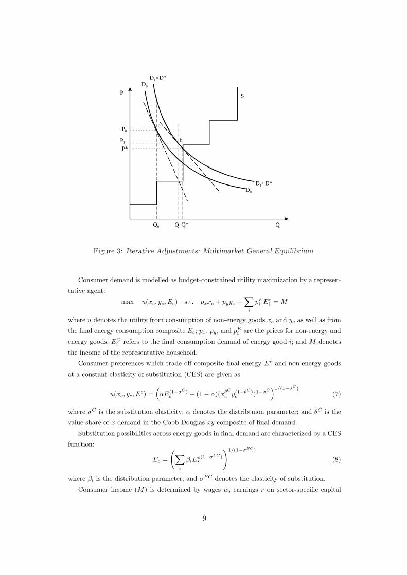
Figure 3 illustrates the same procedure for a multi-market general equilibrium in which
shifts in the demand for one good induce changes in the demand for other goods through
general equilibrium income and cross-market price effects. At the benchmark point we have
an energy demand function D0 − D0 which is locally approximated by a linear demand
function at point a. At the next iteration, changes in energy supplies and associated general
equilibrium effects lead to the energy demand function D1−D1 which is approximated locally
at b.
7
P*
QQ0 Q1Q*
P
P0
P1
S
D
D
a
b
c1
Figure 2: Iterative Adjustments: Single Market Partial Equilibrium
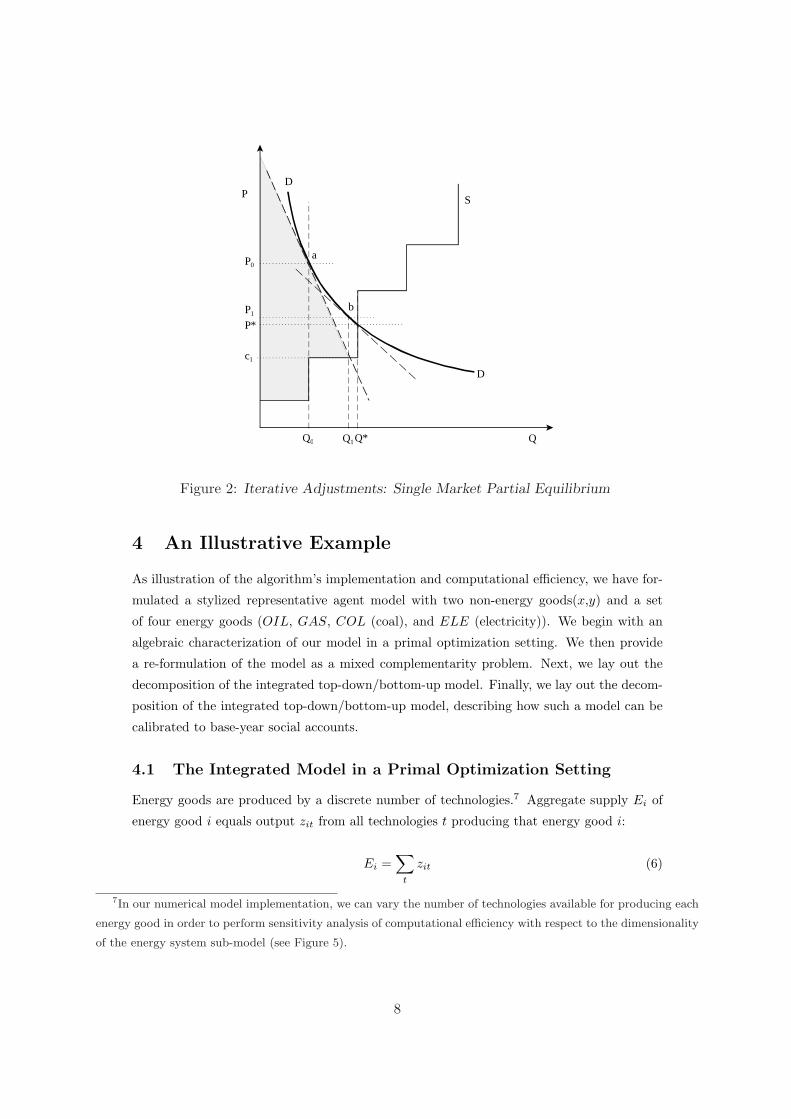
4 An Illustrative Example
As illustration of the algorithm’s implementation and computational efficiency, we have for-
mulated a stylized representative agent model with two non-energy goods(x,y) and a set
of four energy goods (OIL, GAS, COL (coal), and ELE (electricity)). We begin with an
algebraic characterization of our model in a primal optimization setting. We then provide
a re-formulation of the model as a mixed complementarity problem. Next, we lay out the
decomposition of the integrated top-down/bottom-up model. Finally, we lay out the decom-
position of the integrated top-down/bottom-up model, describing how such a model can be
calibrated to base-year social accounts.
4.1 The Integrated Model in a Primal Optimization Setting
Energy goods are produced by a discrete number of technologies.7 Aggregate supply Ei of
energy good i equals output zit from all technologies t producing that energy good i:
Ei =∑
t
zit (6)
7In our numerical model implementation, we can vary the number of technologies available for producing each
energy good in order to perform sensitivity analysis of computational efficiency with respect to the dimensionality
of the energy system sub-model (see Figure 5).
8
P*
QQ0 Q1 Q*
P
P0
P1
S
D0
a
b
D0
D1.D*
D1.D*
Figure 3: Iterative Adjustments: Multimarket General Equilibrium
Consumer demand is modelled as budget-constrained utility maximization by a represen-
tative agent:
max u(xc, yc, Ec) s.t. pxxc + pyyx +∑
i
pEi Ec
i = M
where u denotes the utility from consumption of non-energy goods xc and yc as well as from
the final energy consumption composite Ec; px, py, and pEi are the prices for non-energy and
energy goods; ECi refers to the final consumption demand of energy good i; and M denotes
the income of the representative household.
Consumer preferences which trade off composite final energy Ec and non-energy goods
at a constant elasticity of substitution (CES) are given as:
u(xc, yc, Ec) =
(αE(1−σC)
c + (1− α)(xθC
c y(1−θC)c )1−σC
)1/(1−σC)
(7)
where σC is the substitution elasticity; α denotes the distribtuion parameter; and θC is the
value share of x demand in the Cobb-Douglas xy-composite of final demand.
Substitution possibilities across energy goods in final demand are characterized by a CES
function:
Ec =
(∑
i
βiEci(1−σEC)
)1/(1−σEC)
(8)
where βi is the distribution parameter; and σEC denotes the elasticity of substitution.
Consumer income (M) is determined by wages w, earnings r on sector-specific capital
9
and scarcity rents uit on capacities of energy technology t producing energy good i:
M = rxKx + ryKy + wL +∑
it
µitzit (9)
where Ky, Kx denote sector-specific (fixed) capital; L is the fixed labor supply; and zit
denotes the capacity constraint on technology t producing energy good i.
Goods x and y enter intermediate demand to energy production and final consumption
demand:
x =∑
it
axitzit + xc (10)
y =∑
it
ayitzit + yc (11)
where ayit (ax
it) denote the (per-unit) input coefficient of non-energy input to the production
of energy good i by technology t; zit is the activity level of technology t delivering energy
good i.
Energy supplies enter as intermediate inputs into the production of non-energy goods and
final demand. Furthermore energy supplies serve as intermediate inputs to the production
of other energy goods. 8 The market clearance condition for energy good i is:
Ei = Exi + Ey
i + Eci +
∑
i′t
bii′tzi′t (12)
where bii′t is the input coefficient of energy good i into technology t producing energy good
i′.
The labor market is cleared by the real wage w:
Lx + Ly = L (13)
Likewise, rental rates rx and ry clear sector-specific capital markets:
Kx = Kx (14)
Ky = Ky (15)
Upper bounds on energy sector technologies are realized through adjustment of technology-
specific rents µit:
0 ≤ zit ≤ zit (16)
Production of non-energy goods x and y is based on profit maximization subject to
technical constraints:
max pxx− wLx +∑
i
pEi Ex
i s.t. x = fx(Kx, Lx, gx(Ex))
8Coal and gas serve as inputs to the production of electricity, crude oil is refined into transportation fuels, etc.
10
and
max pyy − wLy +∑
i
pEi Ey
i s.t. y = fy(Ky, Ly, gy(Ey))
Three-level nested separable CES functions characterize trade-offs between primary fac-
tors and energy in the production of goods x and y. At the top level, an energy composite is
combined with a Cobb-Douglas aggregate in labor and capital subject to a constant elasticity
of substitution:
fi(Ki, Li, Ei) = φi
(γiE
(1−σi)i + (1− γi)Kθ
i L(1−θi)(1−σi)i
)1/(1−σi)
i ∈ {x, y}
where φi is the efficiency parameter, γi is the distribution parameter, and σi is the elasticity
of substitution.
At the lower level, energy inputs are combined (to a sector-specfic energy input composite
Ei) in a manner which distinguishes the differences in substitutability between electricitiy,
coal, oil, and gas:
Ei = Eθele
iele,i
(δiE
(1−σEi )
col,i + (1− δi)(Eθi,oil
oil,i E(1−θi,oil
gas,i )(1−σEi )
)(1−θelei )/(1−σE
i )
i ∈ {x, y}
where θelei is the value share of electricity in the Cobb-Douglas energy composite demand
of sector i; δi is the distribution parameter; θoili refers to the value share of oil in the Cobb-
Douglas oil-gas composite; σEi denotes the substituion elasticity between coal and the oil-gas
composite.
Energy sector supplies are produced by profit-maximizing firms. The technology t that
produces energy good i is then selected at a level which maximizes returns subject to capacity
constraints:
max zit
(pE
i − pxaxit − pyay
it −∑
i′pE
i bi′it
)s.t. zit ≤ zit
4.2 The Integrated Model as a MCP
The model presented above omits a number of complications which arise in applied general
equilibrium models. These might include multiple consumers with distinct preferences, taxes
(on energy, goods or factor incomes), knowledge spillovers, or imperfect competition. In the
absence of these features which typically violate integrability conditions, the integrated model
can be solved as a conventional nonlinear program by maximizing u subject to (6) through
(16). The optimization approach is, however, often too restrictive in terms of the model
features which need to be included for concrete policy analysis.
The complementarity format offers a flexible alternative to non-linear optimization as
a means of representing economic equilibrium models through “canonical” general equillib-
rium conditions (see conditions (1), (2), and (3)). In the MCP framework, the algebraic
representation of our stylised model begins from the dual cost minimization problems of the
individual producers. For sectors i = {x, y} we have cost-minimizing unit energy costs given
by:
11
pEi =
(pele
θelei
)θelei
{δi
(pcol
δi
)(1−σEi )
+(1− δi)[( poil
(1− δi)θoili
)θoili
( pgas
(1− δi)(1− θoili )
)(1−θoili )](1−σE
i )}1/(1−σE
i )
Unit profit functions for x and y are in turn given by:
Πi = pi − 1φi
[γi
(pEi
γi
)(1−σi)
+(1− γi)( ri
θi(1− γi)
)θi(1−σi)( w
(1− θi)(1− γi)
)(1−θi)(1−σi)]1/(1−σi)
The unit cost of energy inputs to final demand are given by:
pEc =
(∑
i
βi
(pE
i
βi
)1−σEC )1/(1−σEC)
and the resulting cost of a unit of final consumption is:
pc =
α
(pE
c
α
)1−σC
+ (1− α)
((px
θC(1− α)
)θC (py
(1− θC)(1− α)
)(1−θC))1−σC
1/(1−σC)
Finally, the unit profit associated with technology t for energy good i = {col, oil, gas, ele}is:
ΠEit = pE
i − pxaxit − pyay
it −∑
i′pE
i bi′it − µit
Given the underlying functional forms, we observe that the complementarity conditions
only will apply for the energy sector technologies and the shadow prices on the associated ca-
pacity constraints; all of the macro economic prices and quantities will be non-zero. By use of
Shepard’s Lemma we can then write the equilibrium as the following mixed complementarity
problem:
• Zero-profit conditions:
zit ≥ zit ⊥ µit ≥ 0 (17)
−ΠEit ≥ 0 ⊥ zit ≥ 0 (18)
Πx = 0 (19)
Πy = 0 (20)
12
• Market clearence conditions:
x =∑
it
axitzit + c
∂Πc
∂px(21)
y =∑
it
ayitzit + c
∂Πc
∂py(22)
L = x∂Πx
∂w+ y
∂Πy
∂w(23)
Kx = x∂Πx
∂rx(24)
Ky = y∂Πy
∂ry(25)
∑t
zit −∑
i′t
bii′tzi′t = c∂Πc
∂pEi
+ x∂Πx
∂pEi
+ y∂Πy
∂pEi
(26)
c =M
pc(27)
• Income balance:
M = rxKx + ryKy + wL +∑
it
µitzit (28)
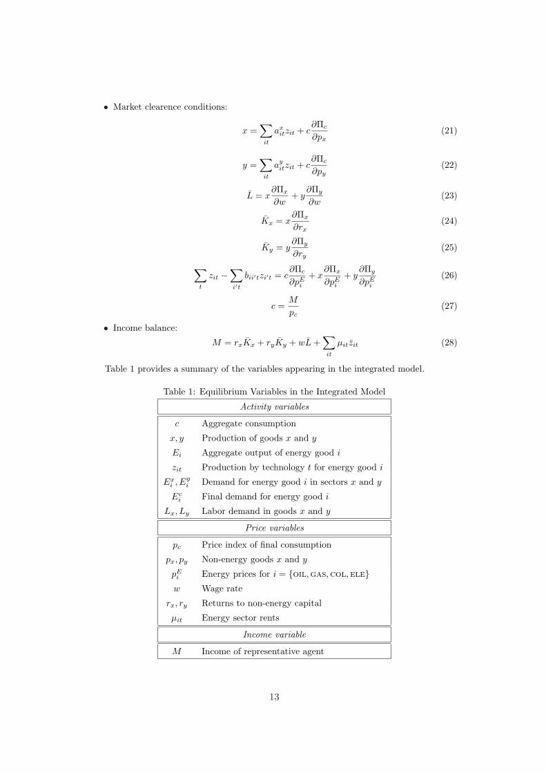
Table 1 provides a summary of the variables appearing in the integrated model.
Table 1: Equilibrium Variables in the Integrated Model
Activity variables
c Aggregate consumption
x, y Production of goods x and y
Ei Aggregate output of energy good i
zit Production by technology t for energy good i
Exi , Ey
i Demand for energy good i in sectors x and y
Eci Final demand for energy good i
Lx, Ly Labor demand in goods x and y
Price variables
pc Price index of final consumption
px, py Non-energy goods x and y
pEi Energy prices for i = {oil,gas,col,ele}w Wage rate
rx, ry Returns to non-energy capital
µit Energy sector rents
Income variable
M Income of representative agent
13
4.3 Decomposition
Our decomposition strategy requires that we separate the integrated model into a top-down
model of the overall economy and a bottom-up model of the energy supply system. Within
the top-down model, we treat net energy system netputs as exogenous. Energy supply
activities are no longer endogenous and we can drop equations (17) and (18). Net energy
supplies and inputs of non-energy goods to the energy system enter the top-down model
as parameters. Parameterized energy-sector netputs Si and inputs xE and yE are valued
at market prices which implicitly include rents on specific energy resources (so we can drop
these from the income constraint). The adjusted market clearance condition for energy goods
within the top-down model is:
Si = Exi + Ey
i + Eci (29)
and the revised market clearance conditions for non-energy goods are:
x = xE + c∂Πc
∂px(30)
and
y = yE + c∂Πc
∂py(31)
The revised income balance (28) reads:
M = rxKx + ryKy + wL +∑
i
pEi Si − pxxE − py yE (32)
The bottom-up model can be represented as a quadratic programming problem in which
the sum of producer and consumer surplus is maximized subject to supply-demand balances
for energy and resource bounds on technologies:
max∑
i pEi (1 + 2Si−Si
2εiSi)− pxxE − pyyE (33)
subject to
Si =∑
t zit −∑
i′t bii′tzi′t
xE =∑
it axitzit
yE =∑
it ayitzit
0 ≤ zit ≤ zit
Table 2 summarizes the additional variables and parameters appearing in the bottom-up
(sub-)model.
14
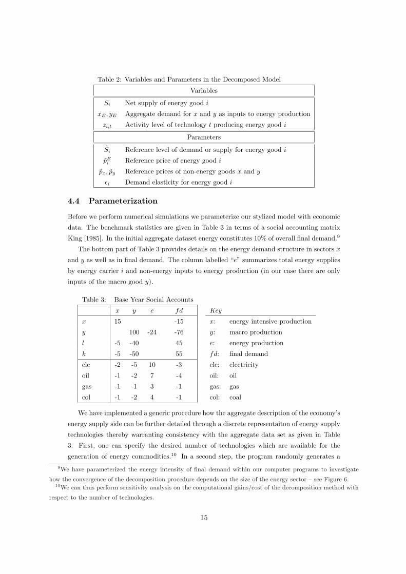
Table 2: Variables and Parameters in the Decomposed Model
Variables
Si Net supply of energy good i
xE , yE Aggregate demand for x and y as inputs to energy production
zi,t Activity level of technology t producing energy good i
Parameters
Si Reference level of demand or supply for energy good i
pEi Reference price of energy good i
px, py Reference prices of non-energy goods x and y
εi Demand elasticity for energy good i
4.4 Parameterization
Before we perform numerical simulations we parameterize our stylized model with economic
data. The benchmark statistics are given in Table 3 in terms of a social accounting matrix
King [1985]. In the initial aggregate dataset energy constitutes 10% of overall final demand.9
The bottom part of Table 3 provides details on the energy demand structure in sectors x
and y as well as in final demand. The column labelled “e” summarizes total energy supplies
by energy carrier i and non-energy inputs to energy production (in our case there are only
inputs of the macro good y).
Table 3: Base Year Social Accounts
x y e fd Key
x 15 -15 x: energy intensive production
y 100 -24 -76 y: macro production
l -5 -40 45 e: energy production
k -5 -50 55 fd: final demand
ele -2 -5 10 -3 ele: electricity
oil -1 -2 7 -4 oil: oil
gas -1 -1 3 -1 gas: gas
col -1 -2 4 -1 col: coal
We have implemented a generic procedure how the aggregate description of the economy’s
energy supply side can be further detailed through a discrete representaiton of energy supply
technologies thereby warranting consistency with the aggregate data set as given in Table
3. First, one can specify the desired number of technologies which are available for the
generation of energy commodities.10 In a second step, the program randomly generates a9We have parameterized the energy intensity of final demand within our computer programs to investigate
how the convergence of the decomposition procedure depends on the size of the energy sector – see Figure 6.10We can thus perform sensitivity analysis on the computational gains/cost of the decomposition method with
respect to the number of technologies.
15

cost distribution for each technology thereby assigning a certain fraction of technologies as
initially idle (non-profitable) at benchmark prices. The cost structure of discrete technologies
– fuel costs and non-energy input costs – is then again assigned randomly; capital earnings,
i.e. scarcity rents on technological capacities, are determined as a residual (if a technology
is initially idle, the initial rents are obviously zero). Finally, relative capacities are randomly
assigned and scaled such that net energy supply equals the given overall economic energy
demand (see Table 3).
Figure 4 illustrates the step-wise energy supply structure by technologies in merit order for
the different energy commodities (the number of available technologies has been set to 10 in
this example). At benchmark energy prices of unity, the break-even “point” for technologies
is at marginal costs of 1 – all technologies that are more expensive will be initially inactive.
0.8
0.85
0.9
0.95
1
1.05
1.1
0 2 4 6 8 10 12 14
Mar
gina
l cos
t (B
MK
pri
ce =
1)
Supply quantity
eleoil
gascol
Figure 4: Energy Supply Schedules (Number of Technologies = 20)
4.5 Computational Results
In order to illustrate the potential usefulness of our decomposition approach, we provide
some numerical tests with the calibrated version of our stylized model. As an exogenous
policy shock, we assume a technological breakthrough which reduces non-energy inputs to
non-fossil electricity generation technolgies by a half.
16
The decomposed integrated model is solved iteratively in its top-down and bottom-up
sub-models. After the exogenous policy shock, we may first solve the top-down model. Next,
we solve the bottom-up model taking into account the equilibrium prices of the top-down
model. The solution values of the bottom-up model are subsequently used to update the
quantities on energy system outputs and inputs which enter into the top-down model.
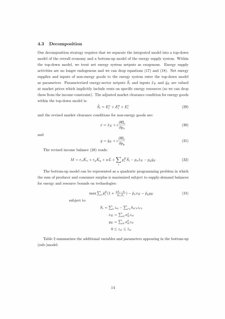
Figure 5 provides some evidence on the computational efficiency of our decomposition
algorithm. We compare the computational cost for the integrated model formulation vis--
vis the decomposed model formulation as a function of the number of energy technologies.
It becomes evident that the decomposition delivers substantial time savings towards an
increasing number of technologies.
Figure 5: Computational Cost of Decomposition
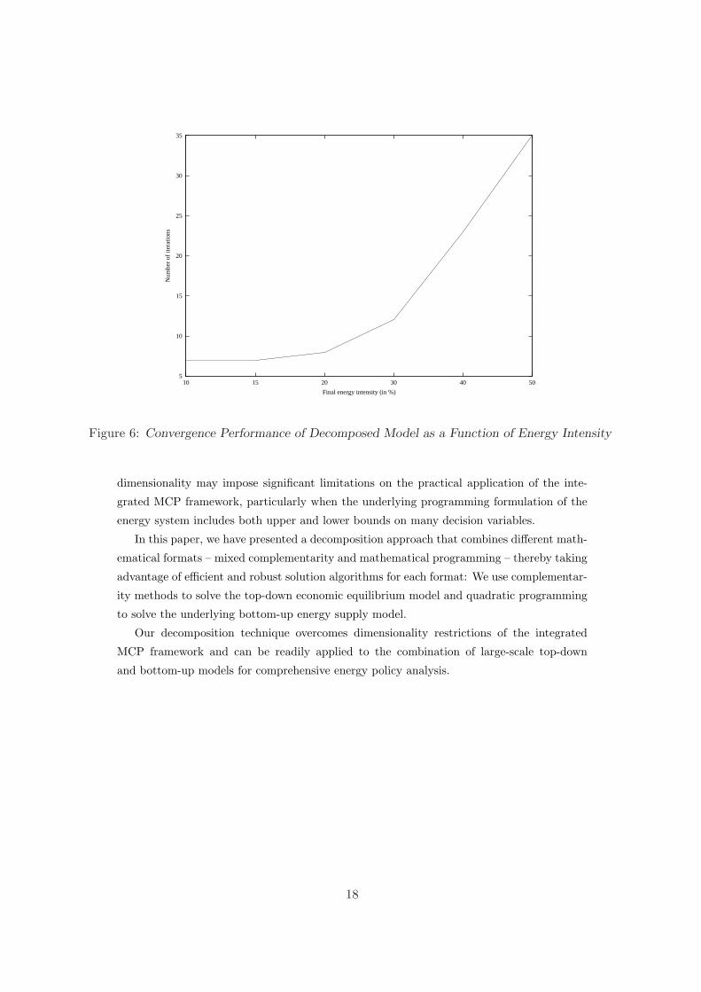
Figure 6 investigates the convergence performance of the decomposed model with re-
spect to the energy intensity of final demand. The graph shows how iterations required for
convergence increase with the size of the energy sector.
5 Conclusions
The combination of bottom-up and top-down approaches constitutes a long-standing chal-
lenge in applied energy policy analysis. The formulation of economic equilibrium conditions
as mixed complementarity problem provides a unifying framework for combining techno-
logical details of bottom-up models and economic richness of top-down models. However,
17
5
10
15
20
25
30
35
10 15 20 30 40 50
Num
ber
of it
erat
ions
Final energy intensity (in %)
Figure 6: Convergence Performance of Decomposed Model as a Function of Energy Intensity
dimensionality may impose significant limitations on the practical application of the inte-
grated MCP framework, particularly when the underlying programming formulation of the
energy system includes both upper and lower bounds on many decision variables.
In this paper, we have presented a decomposition approach that combines different math-
ematical formats – mixed complementarity and mathematical programming – thereby taking
advantage of efficient and robust solution algorithms for each format: We use complementar-
ity methods to solve the top-down economic equilibrium model and quadratic programming
to solve the underlying bottom-up energy supply model.
Our decomposition technique overcomes dimensionality restrictions of the integrated
MCP framework and can be readily applied to the combination of large-scale top-down
and bottom-up models for comprehensive energy policy analysis.
18
References
Bergmann, L., “The Development of Computable General Equilibrium Models,” in
L. Bergman, D. W. Jorgenson, and E. Zalai, eds., General Equilibrium Modeling and
Economic Policy Analysis, Cambridge, 1990, pp. 3–30.
Bohringer, C., “The Synthesis of Bottom-Up and Top-Down in Energy Policy Modeling,”
Energy Economics, 1998, 20 (3), 233–248.
, A. Muller, and M. Wickart, “Economic Impacts of a Premature Nuclear Phase-Out
in Switzerland,” Swiss Journal of Economics and Statistics, 2003, 139 (4), 461–505.
and T.F. Rutherford, “Integrating Bottom-Up into Top-Down:A Mixed Comple-
mentarity Approach,” Discussion Paper No. 05-28, ZEW, Mannheim 2005.
Cottle, R. W. and J.-S. Pang, The Linear Complementarity Problem, Academic Press,
1992.
Dirkse, S. and M. Ferris, “The PATH Solver: A Non-monotone Stabilization Scheme
for Mixed Complementarity Problems,” Optimization Methods & Software, 1995, 5,
123–156.
Frei, C.W., P.-A. Hadi, and G. Sarlos, “Dynamic formulation of a top-down and
bottom-up merging energy policy model,” Energy Policy, 2003, 31 (10), 1017–1031.
Hudson, E.A. and D.W. Jorgenson, “US energy policy and economic growth, 1975-
2000,” The Bell Journal of Economics and Management Science, 1974, 5, 461–514.
International Panel on Climate Change (IPCC), Climate Change, 1995: Economic
and Social Dimensions of Climate Change – Contribution of Working Group II to the
Second Assessment Report of the Intergovernmental Panel on Climate Change, Cam-
bridge, 1996.
King, B., “What is a SAM?,” in “Social Accounting Matrices: A Basis for Planning,”
Washington D. C.: The World Bank, 1985.
Manne, A.S. and T.F. Rutherford, “International trade, capital flows and sectoral anal-
ysis: formulation and solution of intertemporal equilibrium models,” in W.W. Cooper
and A.B. Whinston, eds., New Directions in Computational Economics, Springer, 1994,
pp. 191–205.
Mathiesen, L., “Computation of Economic Equilibrium by a Sequence of Linear Comple-
mentarity Problems,” in A. Manne, ed., Economic Equilibrium – Model Formulation
and Solution, Vol. 23 1985, pp. 144–162.
Rutherford, T. F., “Extensions of GAMS for Complementarity Problems Arising in Ap-
plied Economics,” Journal of Economic Dynamics and Control, 1995, 19, 1299–1324.
19
Recommended