Download pdf - Combining the Stochastic Counterpart and Stochastic Approximation Methods

Discrete Event Dynamic Systems: Theory and Applications, 7, 5–28 (1997)c© 1997 Kluwer Academic Publishers, Boston. Manufactured in The Netherlands.

Combining the Stochastic Counterpartand Stochastic Approximation Methods

JEAN-PIERRE DUSSAULT [email protected] de mathematiques et informatique, Universite de Sherbrooke,Sherbrooke J1K 2R1, Canada

DONALD LABRECQUE AND PIERRE L’ECUYER [email protected] d’IRO, Universite de Montreal,C.P. 6128, Succ. Centre-Ville, Montreal H3C 3J7, Canada

REUVEN Y. RUBINSTEIN [email protected] of Industrial Engineering and ManagementTechnion—Israel Institute of Technology, Haifa 32000, Israeland Department of Mathematics, EPFL-EcublensCH-1015 Lausanne, Switzerland

Received June 23, 1993; Revised May 16, 1995; Accepted April 25, 1996

Abstract. In this work, we examine how to combine the score function method with the standard crude MonteCarlo and experimental design approaches, in order to evaluate the expected performance of a discrete eventsystem and its associated gradientsimultaneouslyfor different scenarios (combinations of parameter values), aswell as to optimize the expected performance with respect to two parameter sets, which represent parameters ofthe underlying probability law (for the system’s evolution) and parameters of the sample performance measure,respectively. We explore how the stochastic approximation and stochastic counterpart methods can be combinedto perform optimization with respect to both sets of parameters at the same time. We outline three combinedalgorithms of that form, one sequential and two parallel, and give a convergence proof for one of them. We discussa number of issues related to the implementation and convergence of those algorithms, introduce averaging variants,and give numerical illustrations.

Keywords: Score function, sensitivity analysis, optimization, stochastic counterpart, stochastic approximation.

1. Introduction

Let

`(v, θ) = Ev{L(Y, θ)} (1)

be the expected performance of a discrete event system (DES), whereL is the sampleperformance driven by an input vectorY , which has a probability density function (pdf)f(y, v). In (1),f andL depend on the vectors of parametersv andθ, respectively, and thesubscriptv inEv means that the expectation is taken with respect tof(·, v). In other words,v is a parameter of the probability law, whileθ is a parameter of the sample performance.We assume that`(v, θ) is not available analytically and that we need to resort to Monte Carlosimulation methods for its estimation. We are concerned with the following questions:

6 DUSSAULT, ET AL.

(i) Solve the so-called “what-if” problem; that is, to estimate`(v, θ) and its gradient w.r.t.v andθ, ∇v`(v, θ) and∇θ`(v, θ), in functional form, or simultaneously for differentvalues ofv andθ;

(ii) Combine the Crude Monte Carlo (CMC) and the score function (SF) methods, to dealwith parametersθ andv, respectively;

(iii) Solve an optimization problem associated with`(v, θ), where bothv andθ are decisionparameters.

As a motivating example, consider a queueing network containingGI/D/1 orGI/G/c/mqueues, wherec andm denote the number of parallel servers and the buffer size, respec-tively. In the first case,v might be a parameter (vector) of the interarrival pdff(y, v) andθmight be the vector of (fixed) service times, while in the second case,v might be the vectorof the interarrival and service rates in the joint pdff(y, v) andθ might be the vector of thebuffer size and the number of parallel servers, respectively.

In its original form, the likelihood ratio (LR) or score function (SF) method (Glynn,1990, Reiman and Weiss, 1989, Rubinstein, 1976, Rubinstein, 1986, Rubinstein, 1992Rubinstein and Shapiro, 1993) permits the solution of the “what-if” problem from asin-gle simulation run(single sample path) with respect tov alone, that is, whenθ is fixed.Roughly, the use of the score function transforms an estimator of`(v, θ) into an estimatorof ∇v`(v, θ), whereas the likelihood ratio transforms point estimators into functional esti-mators, thereby allowing the estimation of the entire functions`(·, θ) and∇v`(·, θ) froma single simulation run, for any given value ofθ. The latter “likelihood ratio” or “changeof measure” technique is in fact exactly the same as that used inimportance samplingforvariance reduction (Glynn and Iglehart, 1989). Unlike SF, the CMC method permits thesolution of the “what-if” problem with respect to bothv andθ, simply by performing sepa-rate simulations at each parameter values of interest. Since it requiresmultiple runs(at leasta separate run for each point(v, θ)), it is typically time-consuming. Note that a modifi-cation of the SF method, the so-called “push out” method (Rubinstein and Shapiro, 1993),as well as the perturbation analysis (PA) method (Glasserman, 1991), also called “pushin” method in (Rubinstein and Shapiro, 1993), combined with the use of a likelihood ratio,permit (in many cases) the solution of the “what-if” problemsimultaneously from a singlesimulationwith respect to bothv and θ; see (L’Ecuyer, 1993) for examples. Here, weshall not deal with the latter approaches. We should mention that the SF method some-times suffers from a variance explosion problem (the variance of the estimator may becomehuge at some values), especially when the values ofv of interest span a large area (see(L’Ecuyer, 1993, Rubinstein and Shapiro, 1993) for details). But there are ways of dealingwith such problems (e.g., break the area of interest into smaller subareas), at least for certainclasses of applications (Rubinstein and Shapiro, 1993).

Suppose now that we want to minimize`(v, θ) with respect tov andθ. One approachfor minimizing `(v, θ) w.r.t. v for fixedθ is to compute an estimator of`(·, θ) in functionalform, using a likelihood ratio, based onN replicates of the simulation, and then minimizethe (sample) value of that estimator w.r.t.v using conventional mathematical programmingtools. The latter minimization problem is called thestochastic counterpart(SC). That SCoptimization approach is studied in much detail in Rubinstein and Shapiro (1993), where

STOCHASTIC COUNTERPART AND STOCHASTIC APPROXIMATION METHOD 7

it is shown that the sample optimizer converges to the true optimizer with probability one(w.p. 1), and obeys a central-limit theorem, as the sample sizeN goes to∞. If the numberof values ofθ of interest is finite and not too large, then the SC approach can be applied ateach such value, and one may select the value ofθ which gave the best result. A statisticalanalysis of such an approach can be performed along the lines of the statisticalrankingand selectionandmultiple comparisonmethods (Goldsman, Nelson, and Schmeiser, 1991,Law and Kelton, 1991, Yang and Nelson, 1991). In particular, those values ofθ of interestmay have been chosen among a much larger (perhaps infinite) set by someexperimentaldesign(ED) strategy (Kleijnen and Van Groenendaal, 1992).

Suppose now that both parameters are continuous. To optimize w.r.t.θ for fixedv, one canuse a stochastic approximation (SA) algorithm (see, e.g., (Ermoliev, 1983, Ermoliev andGaivoronski, 1992, Kushner and Clark, 1978, L’Ecuyer and Glynn, 1994, Pflug, 1990, Pflug,1992, Polyak and Juditsky, 1992, Rubinstein, 1986) and several further references giventhere). SA is an iterative procedure which at each step estimates the gradient of the objectivefunction and makes a small step in its opposite direction. The gradient estimator can bebased on either SF, PA, finite differences, and so on, and the speed of convergence dependshighly on the quality of the gradient estimator that is used (for example, is can be quiteslow when using the so-called Kiefer-Wolfowitz SA variant, based on finite differenceswith independent random numbers). In fact, the SA algorithm can be used as well foroptimization w.r.t.v, or w.r.t. both parameters simultaneously. However, it could be in somecases more efficient or convenient to use the SC approach rather than SA for dealing withv. This leads to the following question: Can we design combined (or hybrid) algorithmswhich use SC forv and SA forθ, while performing optimization w.r.t. both parameterssimultaneously ?

The rest of this work is organized as follows. In Section 2, we show how to combine the SFand CMC/ED methods in order to estimate`(v, θ),∇v`(v, θ), and∇θ`(v, θ) simultaneouslyfor several scenarios (combinations) of(v, θ). Section 3 deals with the minimization of`(v, θ) with respect to bothv andθ. We outline three optimization algorithms, each comingin two versions, and provide a convergence proof for the first version of the first algorithm.A numerical example then gives some insight into the behavior of the algorithms and alsoillustrates some potential difficulties.

2. The “What-if” Problem

In this section, we recall some background material on the SF method and on how a func-tional estimator w.r.t.v can be obtained. Further details on this are given in (Asmussen andRubinstein, 1992a, Asmussen and Rubinstein, 1992b, Asmussen, Rubinstein, and Wang,1994, Glynn and Iglehart, 1989, Glynn, 1990, L’Ecuyer, 1990, Reiman and Wiess, 1989,Rubinstein, 1992, Rubinstein and Shapiro, 1993) We then explain how to combine SF andCMC in order to estimate(v, θ) and its gradientsimultaneouslyfor several values ofv andθ. We distinguish the following two cases: (a)θ is fixed; (b) θ is not fixed.

8 DUSSAULT, ET AL.

2.1. The Case of a Fixedθ: a “What-if” Design with Respect tov

Assume thatθ is fixed and letY1, Y2, . . . , be an input sequence of independent identicallydistributed (iid) random vectors, generated from a densityf(·, v), which depends on theparameter vectorv. Let {Lt : t > 0} be a discrete-time output process driven by{Yt},that is,Lt = Lt(Y1, . . . , Yt, θ). Assume that{Lt} is regenerative with cycle lengthτ =τ(Y1, Y2, . . . , θ). It is well known (Wolff, 1989) that the expected steady-state (average) of{Lt} can be written as

`(v, θ) =Ev [

∑τt=1 Lt]

Ev[τ ]=`1(v, θ)

`2(v, θ), (2)

provided thatEv[τ ] > 0 andEv [|∑τt=1 Lt|] <∞, and similarly whenLt is a continuous-

time regenerative process. A finite-horizon model can be viewed as a special case of this:just replace 2(v, θ) by 1.

Under standard regularity conditions allowing interchangeability of expectation and dif-ferentiation (e.g., uniform integrability), one has (Asmussen and Rubinstein, 1992a,Glynn and Iglehart, 1989, L’Ecuyer, 1990, Rubinstein and Shapiro, 1993):

`1(v, θ) = Eg

[τ∑t=1

LtWt

]; (3)

∇v`1(v, θ) = Eg

[τ∑t=1

Lt∇vWt

], (4)

whereLt = Lt(Z1, . . . , Zt, θ), Wt =∏tj=1 f(Zj , v)/g(Zj), (Z1, . . . , Zt) has density∏t

j=1 g(zj), g(·) is a density that dominates all thef(·, v)’s in the sense thatf(z, v) > 0for somev implies g(z) > 0, andEg denotes the expectation with respect tog. Toobtain similar expressions for2, just replaceLt by 1. We callWt, ∇Wt, LtWt, andLt∇Wt the likelihood ratio, score function, sample performance, and sensitivitypro-cesses, respectively. This could also be generalized to larger values ofk (L’Ecuyer, 1990,Rubinstein and Shapiro, 1993).

If we further assume that∇θLt(θ) is available from the simulation, that∇θτ = 0 (which istypical, sinceτ is usually piecewise constant as a function ofθ), and under a few additionalconditions (see (Glasserman, 1991, Heidelberger, et al., 1988)), then one also has

∇θ`1(v, θ)− `1(v, θ)∇θ`2(v, θ) = Eg

[τ∑t=1

Wt∇θLt

]. (5)

(Note that the latter bracketted expression is typicallynotan unbiased estimator of`1(v, θ)whenτ depends onθ.) When these conditions are not satisfied, one can still rely to finitedifferences to estimate the gradients on the left-hand-side of (5), preferably with commonrandom numbers (see (L’Ecuyer and Perron, 1994)).

Remark 1 In this setup, we have implicitly assumed that bothv and θ are continousparameters and that the derivatives exist. In the case where eitherv or θ is discrete, thenwe just forget about the corresponding derivatives.


Consider now a sample ofN iid regenerative cycles, with valuesτi,Lti, andWti of τ ,Lt,andWt, respectively, fort ≥ 1 and1 ≤ i ≤ N , again based on the underlying distributiong.Then, under the conditions mentioned above, unbiased estimators of`1(v, θ) and∇v`1(v, θ)are given by

`1N (v, θ) =1

N

N∑i=1

τi∑t=1

LtiWti,

∇v`1N (v, θ) =1

N

N∑i=1

τi∑t=1

Lti∇vWti,

and similarly for 2 withLti replaced by 1. Consistent estimators of`(v, θ) = `1(v, θ)/`2(v, θ)and∇v`(v, θ) = (∇v`1(v, θ)− `(v, θ)∇v`2(v, θ))/`2(v, θ) are then given by:

`N (v, θ) =`1N (v, θ)

`2N (v, θ)(6)

and

∇v`N (v, θ) =∇v`1N (v, θ)− `N (v, θ)∇v`2N (v, θ)

`2N (v, θ)(7)

respectively. Note that these estimators depend onv only through theWti’s, which cantypically be written explicitly as functions ofv for fixed values of the underlying randomvariablesZji’s. These estimators then permit one to estimate the function and its gra-dient in functional form w.r.t.v, from the simulation ofN regenerative cycles based ondensityg. Confidence intervals at any fixed value ofv can be computed as explained in(Glynn, L’Ecuyer, and Adès, 1991). In a similar way, again under the appropriate condi-tions, a consistent estimator of∇θ`(v, θ) is given by

∇θ`N (v, θ) =∇θ`1N (v, θ)

`2N (v, θ). (8)

2.2. Selecting the Reference Parameter Value

An important question in this context is how to selectg. Henceforth, we shall assume thatg(·) = f(·, v0), wherev0 is a fixed value ofv called thereference parameter value. Nowthe question is how to selectv0. This has been studied, e.g., in Asmussen and Rubinstein(1992b), L’Ecuyer (1993), Rubinstein and Shapiro (1993). A good choice ofv0 turns outto be extremely important, because for a givenv, the variance of the estimators (6–8) mayblow up to a very large value or even become infinite for certain choices ofv0. A goodchoice ofv0 may reduce the variance at a givenv compared to that obtained withv0 = v(the usual choice in standard simulation). On the other hand, it may happen that for anygiven value ofv0, the variance blows up for certain values ofv.

Solving the problem:

10 DUSSAULT, ET AL.

minv0∈V

Varv0 [`N (v, θ)], (9)

for a givenv ∈ V is very difficult in general. In our context, we are also interested in a valueof v0 that does well for all values ofv in a certain region. Asmussen and Rubinstein (1992b)and Rubinstein and Shapiro (1993) have studied the problem (9) in the context where`(v, θ)is the average sojourn time per customer in a single queue. In that context, letρ(v) denote thetraffic intensity (which is assumed to depend onv). Under conditions given in Rubinsteinand Shapiro (1993), Varv0

[`N (v, θ)] is strictly convex w.r.t.v0 and one hasρ(v∗0) > ρ(v),wherev∗0 is the optimal solution of (9). This means that it is best to simulate at a largertraffic intensity than the one at which we want to estimate the performance or its gradient.The trace of the variance of∇v`N (v, θ) has the same property under similar conditions.Under these conditions, for a givenv, there exists a traffic intensityρ > ρ = ρ(v) such that

Varv0[`N (v, θ)] ≤ Varv[`N (v, θ)] (10)

if and only if ρ(v0) ∈ [ρ, ρ], and similarly for the trace of the variance of∇v`N (v, θ).Conversely, for a fixedρ0 = ρ(v0), there exists an interval[ρ, ρ0], such that

Varv0[`N (v, θ)] ≥ Varv[`N (v, θ)] (11)

for all v such thatρ(v) ∈ [ρ, ρ0]. When going belowρ and aboveρ0, the variance of the“what-if” estimator`N (v, θ) typically increases rather slowly and very fast, respectively,w.r.t. ρ. Similar results were obtained for more complex queueing models for which theperformance measure is the average sojourn or waiting time. A general recommendationfrom (Asmussen and Rubinstein, 1992b, Rubinstein and Shapiro, 1993) is: in order to beon the safe side one should choosev0 such thatρ(v0) is moderately larger than the nominalvalueρ = ρ(v). That does not tell us the precise value ofv∗0 in general, but gives us somerough guideline for that particular class of models.

Example 1 Suppose that the performance measure of interest is the average sojourn time inanM/M/1 queue with traffic intensityρ = ρ(v). In this case,ρ can be found analytically asa function ofρ (Asmussen and Rubinstein, 1992b). For example, ifρ = 0.5, thenρ ≈ 0.8,so that the variance is reduced forρ0 ∈ [ρ, ρ] ≈ [0.5, 0.8], which is a rather broad interval.Conversely, forρ0 = 0.8, we obtain variance reduction in the sense of (11)simultaneouslyfor all ρ ∈ [0.5, 0.8].

Example 2 LetLt(θ) be the expected waiting time for thet-th customer in aGI/D/1 queueand assume that we want to estimate the gradient of the steady-state waiting time,∇θ`(v, θ),whereθ is the (deterministic) service time. To do so, recall first (see (Suri and Zazanis, 1988))that for a GI/G/1 queue, fort ≤ τ , one has

Lt(θ) =t−1∑j=1

(Yj −Aj),

whereτ = min{t : Lt(θ) ≤ 0}, Yj andAj are the service time of customerj and theinterarrival time between customersj− 1 andj, respectively. For the GI/D/1 queue,Lt(θ)reduces to


Lt(θ) =t−1∑j=1

(θ −Aj). (12)

DifferentiatingLt(θ) with respect toθ, we obtain

∇θLt(θ) =t−1∑j=1

(1−Aj). (13)

Substituting finallyLt(θ) and∇θLt(θ) from (12) and (13) into (8), we obtain the estimator∇θ`N (v, θ) which allows the estimation of∇θ`(v, θ) from a single simulation, simultane-ously for different valuesv, for a fixedθ.

Now, letθ be fixed, while we are interested in estimating at valuesv1, . . . , vr1 of v in V .In this case we are interested in the following extension of problem (9):

minv0∈V

maxv=v1,...,vr1

Varv0[`N (v, θ)]. (14)

Arguing as before, again in the same queueing context, it seems natural to choose thereference parameterv0 in such a way that

ρ(v0) ≈ ρ+ = maxk=1,...,r1

ρ(vk), (15)

which means that the reference parameterv0 should correspond to thehighest traffic intensityamong all traffic intensities associated with the selected valuesv1, . . . , vr1 . Of course, itmay happen thatρ− = mink=1,...,r1 ρ(vk) < ρ, in which case the variance is decreasedin the sense of (11) wheneverρ = ρ(vk) is in [ρ, ρ+], and increased otherwise. In thelatter case, the variance increase is typically moderate whenρ− ρ is not too large and thecycle lengthτ tends to be small (see (Asmussen and Rubinstein, 1992b, L’Ecuyer, 1993)for illustrations). If that is not the case, then the set{v1, . . . , vr1} should be partitioned intosmaller subsets and a differentv0 chosen over each subset.

2.3. Many Values ofθ: the “What-if” Design for Both Parameters

Consider now the estimation of`(v, θ) for the“what-if” design

{(v, θ) = (vk, θj), k = 1, . . . , r1, j = 1, . . . , r2}. (16)

In this case, the CMC method (based onN regenerative cycles) requires a total ofr1r2Nsimulations, whereas a straightforward combination of CMC (forθ) with SF/LR methodrequires onlyr2N simulation runs. The idea is simply to apply the technique used for thecase of a fixedθ to each valueθj of interest, as follows:

a) Select a reference parameterv0,j ;

b) PerformN simulation runs using densityg(·) = f(·, v0,j), atθ = θj , and computeLtiandWti (the latter in functional form) for each runi;

12 DUSSAULT, ET AL.

c) Calculate N (vk, θj) according to (6) fork = 1, . . . , r1.

A trivial adaptation of the above allows also to compute the gradient estimators (7) and (8)over the “what-if” design.

Remark 2 In typical applications, the traffic intensity is often monotone in each componentof v andθ. When this is the case, it is easy to find out the parameter value(v0, θ0) thatgives the largest traffic intensityρ0, and use it as a reference parameter to estimate theperformance atall other parameter values of interest. On the other hand, using the samev0

for all θ of interest is not really necessary.

Remark 3 It is common practice in simulation to use thesame streamof random num-bers while running different scenarios (see, e.g., (Law and Kelton, 1991, L’Ecuyer, 1992,Rubinstein, 1986, Yang and Nelson, 1991)), in order to reduce the variance of the differ-ences across scenarios. In the present context, this means that the same stream of randomnumbers would be used for all values ofj, with proper synchronization, so that the differ-ences between the estimates will be due only to the different parameter values, and not todifferent random numbers.

Remark 4 If θ is a continuous parameter, then the above method can be combined withdifferent standard experimental design (ED) methods, such as the full factorial design, thecentral composite design, and so on, w.r.t. the parameterθ. Such designs turn out to beparticular cases of the above “what-if” design, aimed at fitting a regression curve to theresponse surface(v, θ).

Example 3 Suppose that we want to estimate the steady-state expected waiting time in aGI/G/c/m queue with interarrival rate of 1, for all the combinations ofr1 different valuesof the service ratev andr2 different values of the buffer sizeθ = m. To do so, we selecta v0,j according to (15) for each buffer sizemj from the set{m1, . . . ,mr2}, then run thecorrespondingr2 simulations. Here, the reference parameterv0,j should be the smallestvalue ofv of interest, which (in this case) is the same for allj. In comparison with CMC,the number of runs is reduced fromr1r2 to r2. If one also hasρ ∈ [ρ, ρ0], then a variancereduction is also obtained at the same time. If not, then one may partition the values ofv ofinterest into separate intervals, then select a differentv0 and perform separate simulationsfor each interval. For a more specific illustration, consider anM/M/2/m queue withm ∈ {5, 10, 15} andv ∈ {1.25, 1.5, 2.0, 5.0}. Here, one would choosev0 = 1.25 as thereference parameter value. From numerical experiments with this example, we found thatthe estimator of(v, θ) based on the change of measure is more accurate (has less variance)in the sense of (11) than its CMC counterpart forv ≤ 2, and less accurate forv = 5.0, forall values ofm considered.

3. Optimization

3.1. Discrete Parameters

Consider the minimization problem:


min(v,θ)∈V×Θ

`(v, θ), (17)

whereV × Θ = {vk, θj , k = 1, . . . , r1, j = 1, . . . , r2}. To estimate the minimizer,one can simply estimate(v, θ) at all points ofV × Θ (using perhaps the approach ofSection 2.3), and just select the system with the best sample value. Assuming that there isa single best system, the probability of making the correct decision (choosing the truly bestsystem) under that procedure converges to one asN → ∞, under the (weak) conditionsthat our estimators are consistent. This follows from the strong law of large numbers (seealso (Rubinstein and Shapiro, 1993)). Note however that this does not tell us about theprobability of making the correct decision for a specificN .

For finite sample sizesN , there exists “ranking and selection” procedures for selectingthe best system among a finite number of candidates (herer1 × r2 candidates), but theseprocedures usually assume independence between the performance estimators for the dif-ferent candidates (see (Goldsman, Nelson, and Schmeiser, 1991, Law and Kelton, 1991)).Such procedures will return one of the candidates, which will be the the best system, i.e.,the minimizer of (17), with probability at leastp∗, wherep∗ depends on the difference inperformance between the best and second best systems. Similar selection procedures usingcontrol variates and common random numbers have been proposed and analyzed recently(Yang and Nelson, 1991), but the set of assumptions made for the analysis typically do nothold in the context of the methodology outlines in Section 2.3. Developing ranking andselection procedures for that context is a topic for further research.

3.2. Continuous Parameters

We are interested in the minimization problem:

min(v,θ)∈V×Θ

`(v, θ), (18)

whereV andΘ are continuous parameter sets. Before proceeding further, consider also thefollowing two particular cases of (18):

minv∈V

`(v, θ), for fixedθ ∈ Θ (19)

and

minθ∈Θ

`(v, θ), for fixedv ∈ V. (20)

The problems (19) and (20) are well known in the stochastic optimization literature. Inparticular, we can estimate the optimal solution of (19), sayv∗(θ), by solving itsstochasticcounterpart(SC) (see (Rubinstein and Shapiro, 1993)):

minv∈V

`N (v, θ), (21)

using a conventional mathematical programming method. The statistical properties of theminimizer of (21), which is taken as an estimator ofv∗(θ), are studied in Rubinstein and

14 DUSSAULT, ET AL.

Shapiro (1993). Under reasonable conditions, the function¯N (·, θ) is twice continuously

differentiable, and the minimizer in (21) obeys a central-limit theorem and converges tov∗(θ) asO(N−1/2).

In the second case, ifv is fixed andΘ is a compact and convex set, we can estimate theoptimal solution of (20), sayθ∗(v), by using a conventional stochastic approximation (SA)algorithm of the following form:

θn+1 := πΘ[θn − γnψn], (22)

whereπΘ denotes the projection on the convex setΘ, ψn is an estimator of∇θ`(v, θ)at θ = θn (computed at iterationn of the SA algorithm),θn is the parameter valueat the beginning of iterationn, and {γn} is a sequence of gains, decreasing to zero,and such that

∑∞n=1 γn = ∞. A common choice for the sequence of gains isγn =

γ0/n, for some appropriate constantγ0. Under a few additional conditions, the SA al-gorithm can be shown to converge to the optimizer w.p.1, and convergence rates canalso be obtained in several cases; see (Ermoliev, 1983, Ermoliev and Gaivoronski, 1992,Kushner and Clark, 1978, L’Ecuyer and Yin, 1994, Polyak and Juditsky, 1992) and othernumerous references given there. The use of SA and other similar stochastic iterativemethods which use gradient or subgradient estimates in the context of on-line or sim-ulated discrete-event dynamic systems has attracted much attention recently; see, e.g.,(Ermoliev and Gaivoronski, 1992, L’Ecuyer and Glynn, 1994, L’Ecuyer, Giroux, andGlynn, 1994, Plambeck et al., 1993) and the several other references given there.

Remark 5 Here, to simplify the discussion, we have assumed thatγn is a scalar. How-ever, it can also be a matrix of the same dimension asθ. Indeed,γn = γ0/n, whereγ0 is the inverse of the Hessian at the optimum, is asymptotically optimal under broadconditions (Kushner and Clark, 1978). That inverse is of course unknown in practice, butadaptive algorithms have been designed which modify bothθn andγn (adaptively) be-tween iterations. Other techniques (e.g., averaging) can also improve the performance ofSA. For further details, see (Kushner and Clark, 1978, L’Ecuyer, Giroux, and Glynn, 1994,Polyak and Juditsky, 1992, Uryas’ev, 1992) and the references given there.

Let us now turn back to the problem (18). Besides straightforward SA (22), which canbe applied to estimate the parameter vector(v∗, θ∗), we shall present three new algorithmsbased on the programs (19) and (20), which combine SA with the SC method. As we shallsee below, those algorithms work iteratively, but differ from each other by the fact that thefirst algorithm tries to solve the problems (19) and (20) by iterating onv andθ sequentially,in a Gauss-Seidel-like manner, while the other two perform parallel iterations with respectto both groups of variables, in a Jacobi-like manner. The second algorithm is similar to thealgorithm with Relaxationused in games theory (see, e.g., (Bas¸ar, 1987)).

Algorithm 1 : Sequential algorithm

1. Choose two sequences of positive integers:{Mi, i ≥ 1} and{Ni, i ≥ 1}, and threesequences of positive real numbers:{βi, i ≥ 1}, {εi, i ≥ 1}, and{γn, n ≥ 1},following the guidelines given by Assumption 1 below and the remarks that follow.


Choose an initial parameter vector(v1, θ1), which represents our best guess of(v∗, θ∗).Let i := 1, n := 1, andθ1 = θ1.

2. REPEAT

(a) For v fixed atvi, perform SA forMi iterations to improve the current value ofθ,i.e., repeat the followingMi times: Compute a gradient estimatorψn w.r.t. θ bysimulating at parameter value(vi, θn), let

θn+1 := πΘ[θn − γnψn], (23)

and increasen by 1.

(b) Let

θi+1 := θn. (24)

Simulate the system at some reference parameter valuev0,i (which may depend onvi), with θ fixed atθi+1, for Ni regenerative cycles, and then solve the stochasticcounterpart (21). Letv∗i be the solution andvi an approximation of it, such that‖vi − v∗i ‖2 ≤ εi. Put

vi+1 := βivi + (1− βi)vi = vi + βi(vi − vi) (25)

and increasei by 1.

UNTIL an appropriate stopping criterion is met.

3. Return(vi, θi) as an estimate of the optimal solution(v∗, θ∗).

Algorithm 2 : Parallel algorithm I

Same as Algorithm 1, except thatθi+1 is replaced byθi in step 2b. With that modification,steps 2a and 2b can be performed in parallel.

Algorithm 3 : Parallel algorithm II

Same as Algorithm 1, except that (a–b) in step 2 are replaced by the following. Select areference parameter valuev0,i and repeat the followingMi times: Compute a gradientestimatorψn by simulating at parameter value(v0,i, θn), computeθn+1 from (23),and increasen by 1. Then, solve the stochastic counterpart (21) built from the dataobtained during the lastMi SA iterations, assuming (almost correctly) thatθ was fixedat θi+1 = (1/Mi)

∑nj=n−Mi+1 θj . Let vi be an approximation of the solutionv∗i , such

that‖vi − v∗i ‖2 ≤ εi. Computevi+1 from (25) and increasei by 1.

Algorithms 1 and 2 are stochastic versions of the Gauss-Seidel and Jacobi steepest descentalgorithms for nonlinear optimization, respectively. Algorithm 3 is fundamentally differentin the sense that thesamesimulations are used for both the SA and SC. Therefore, it could

16 DUSSAULT, ET AL.

be more economical. However, its analysis and implementation tend to be more difficult.For example, one difficulty could be the choice ofv0,i, because of the fact thatθn is notfixed during an SC iteration.

For each of those algorithms, we also consider the following “averaging” versions: replace(24) by

θi+1 :=1

Mi

n∑j=n−Mi+1

θj . (26)

We shall call those versions 1’, 2’, and 3’, respectively. In those versions, the valueθi of θthat is used for the SC is theaverageof all values ofθn during the last series of SA iterations,instead of just the lastθn. However, when we go back to SA, we restart from the lastθn.In our empirical investigations, that kind of averaging gave much better results than justtaking the lastθn in the SC as stated in the “regular” versions of the algorithms. However,the convergence proofs appear technically more difficult in that case, mainly because of theswitching back fromθi to θn after the SC.

Remark 6 Under appropriate assumptions, if we suppose thatv∗i converges to some valueasi → ∞, then it is not hard to show by standard SA arguments thatθn must convergew.p.1. Conversely, ifθn converges to some value, then the arguments of Rubinstein andShapiro (1993) can be used to show thatvi must also converges w.p.1 under appropriateconditions. In both cases, if the function is convex and the optimizer is in the interior ofΘ,then the convergence point must be the optimum. However, we want (and we shall) proveconvergence without making any a priori assumption about the convergence of one of thetwo sequences. This entails a little more complication.

We now state a list ofsufficientconditions and give a convergence proof to the optimumunder those conditions. Let∇2` denote the Hessian (matrix) of` and‖ · ‖2 denote theEuclidean norm (or the sum of squares of the elements in the case of a matrix). The vectorsare assumed to be column vectors and the “prime” transposes them into line vectors. Fori = 1, 2, . . ., definemi = 1+

∑i−1j=1Mj , let

∑(i) denote

∑mi+Mi

n=mi+1, and letγi =∑

(i) γn.We can decomposeψn, for n ≥ 1, as

ψn = ∇θ`(vi, θn) + ζn + ξn,

whereE[ξn | vi, θn] = 0 andζn = E[ψn | vi, θn]−∇θ`(vi, θn). The random variableζnrepresents the conditional bias on the gradient estimatorψn at thenth SA iteration, whileξn represents the noise.

Assumption 1 (i) The function (v, θ) is twice continuously differentiable overV × Θ,which is a compact and convex subset of thed-dimensional real space for some integerd, and there is a unique minimizer(v∗, θ∗) which is an interior point ofV ×Θ.

(ii) The Hessian∇2`(v, θ) is positive definite overV ×Θ, with smallest eigenvalue boundedbelow byλmin > 0 and largest eigenvalue bounded above byλmax < ∞, uniformlyoverV ×Θ.


(iii) One hasγn ↘ 0, 0 < βi ≤ 1,∑∞i=1 β

2i /N

2i < ∞, Ni → ∞, βi/(Niγi) → 0,∑∞

i=1 min(βi, γi) =∞, γi/βi ≤ K1, andεi ≤ K1/Ni for some finite constantK1.

(iv) One hasE[ζn] → 0, and ζn → 0 w.p.1 asn → ∞. Also, γnE[‖ξn‖2] → 0,γnE[‖ξn‖2 | vi, θn]→ 0 w.p.1, and

∑∞n=1 γ

2nE[‖ξn‖2] <∞.

(v) W.p.1, N (v, θ) is twice continuously differentiable w.r.t.v and there is a finite constantK2 such that

sup(v0,θ)∈V×Θ

E[‖∇v ¯

N (v∗(θ), θ)‖4 | v0, θ]≤ K2

2/N2. (27)

In many cases,ζn is zero and the conditions on it hold trivially. The last condition inAssumption 1(v) is reasonable in view of the fact that∇v`(v∗(θ), θ) = 0.

Observe that the solutionv∗ of the SC (21) is usuallynot an unbiased estimator of theoptimal solution of the original minimization problem (18), but it is a consistent estimatorunder broad conditions (see (Rubinstein and Shapiro, 1993)). This is why we need to takeNi → ∞. Reasonable choices for the sequences could beNi = N0 + N1i for fixedconstantsN0 andN1, andMi = Ni, which gives an equal part of the budget to the SA andSC “components” of the algorithm. The role ofβi is to introduce a weighted averaging ofthe previous values ofvi instead of just taking the last one. The aim of this is mainly toreduce the variance. For example, one can takeβi = Ni/

∑ij=1Nj , which is equivalent to

taking the weighted average:

vi+1 =

∑ij=1Nj vj∑ij=1Nj

.

Other possibilities include takingβi = β0/(b+ i) for some positive constantsβ0 ≤ b, orβiequals to a constant. The latter corresponds to exponential smoothing. The standard choicefor γn is γn = γ0/n for some constantγ0. Finally, one can takeεi = K1/Ni for someconstantK1. We point out that with the above choices ofNi andγn, and withβi equal toa constant, the condition:βi/(Niγi) → 0 is not satisfied.Nevertheless, that combinationturned out to give the best results in our empirical investigations.

Proposition 1 Under Assumption 1, one has

limi→∞

(‖vi − v∗‖2 + ‖θi − θ∗‖2

)= 0 w.p.1

in Algorithm 1.

Proof: Let ∆i = ‖vi − v∗‖2 + ‖θmi − θ∗‖2 = ‖vi − v∗‖2 + ‖θi − θ∗‖2 and∆i,j =‖vi − v∗‖2 + ‖θmi+j − θ∗‖2, j = 0, . . . ,Mi. Let v∗i = v∗(θi+1), the optimal value ofvwhenθ is fixed atθi+1. For i ≥ 1, 0 ≤ j < Mi, andn = mi + j, define

Dn = ∇θ`(vi, θn),

Sn = 2(Dn − ψn)′(θn − θ∗) + γn‖ψn‖2,Ti = ‖vi − v∗i ‖2,sn = E[Sn | vi, θn],

ti = E[Ti | vi,0, θi+1].

18 DUSSAULT, ET AL.

In the remainder of the proof, we will use the following lemmas.

Lemma 1 There is a constant0 < K3 ≤ 1 such that for all(v, θ) ∈ V ×Θ,

‖v − v∗(θ)‖+∇θ`(v, θ)′(θ − θ∗) ≥ K3(‖θ − θ∗‖2 + ‖v − v∗‖2).

Proof: First, observe that

`(v, θ)− `(v∗, θ∗) = ∇`(v∗, θ∗)′(θ − θ∗v − v∗

)+

1

2

(θ − θ∗v − v∗

)′∇2`(v, θ)

(θ − θ∗v − v∗

)≥ λmin

2(‖θ − θ∗‖2 + ‖v − v∗‖2)

where(v, θ) lies on the line segment joining(v, θ) to (v∗, θ∗). Since` is convex, one has

`(v, θ)− `(v∗, θ∗) ≤ ∇θ`(v, θ)′(θ − θ∗) +∇v`(v, θ)′(v − v∗)= ∇θ`(v, θ)′(θ − θ∗) +∇v`(v∗(θ), θ)′(v − v∗)

+ (v − v∗(θ))′∇2v `(

ˆv, θ)(v − v∗)≤ ∇θ`(v, θ)′(θ − θ∗) + λmax‖v − v∗(θ)‖ · ‖v − v∗‖,

whereˆv lies on the line segment betweenv andv∗(θ). SinceV is compact,‖v − v∗‖ isbounded above, say byK, so that

‖θ − θ∗‖2 + ‖v − v∗‖2 ≤ 2

λmin∇θ`(v, θ)′(θ − θ∗) +

2Kλmax

λmin‖v − v∗(θ)‖, (28)

and the result follows.

Lemma 2 There is a finite constantK4 such that for alli ≥ 1,

ti ≤ K4/Ni w.p.1 and E[T 2i ] ≤ K2

4/N2i . (29)

Proof: Let ¯i denote the sample function that corresponds to (6) obtained at iterationi

with N = Ni. From Assumption 1(i,v) and Taylor’s expansion, for anyθ ∈ Θ, one has

ì(v∗i , θ)− ì(v∗i , θ) = (v∗i − v∗i )′∇vì(v∗i , θ) + (v∗i − v∗i )′∇2

v ì(ui(θ), θ)(v∗i − v∗i )/2

whereui(θ) lies on the line betweenv∗i and v∗i . By definition of v∗i , ì(v∗i , θi+1) −ì(v

∗i , θi+1) ≤ 0. Therefore,

2‖v∗i − v∗i ‖ · ‖∇vì(v∗i , θi+1)‖ ≥ (v∗i − v∗i )′∇2v ì(ui(θi+1), θi+1)(v∗i − v∗i )

≥ λmin‖v∗i − v∗i ‖2,

so

‖v∗i − v∗i ‖ ≤ (2/λmin)‖∇vì(v∗i , θi+1)‖


and, from Assumption 1(v), w.p.1,

E[‖vi − v∗i ‖2 | vi,0, θi+1

]≤ 2

(4

λ2min

E[‖∇vì(v∗i , θi+1)‖2 | vi,0, θi+1

]+ εi

)≤ 8K2

λ2minNi

+2K1

Ni.

Similarly,

E[T 2i ] = E

[‖vi − v∗i ‖4

]≤ 8

(E[‖v∗i − v∗i ‖4

]+ E

[‖vi − v∗i ‖4

])≤ 8

(24

λ4min

E[‖∇vì(v∗i , θi+1)‖4

]+ ε2i

)≤ 128K2

2

λ4minN

2i

+8K2

1

N2i

.

DefineK4 = max(8K2/λ2min + 2K1, 128K2

2/λ4min + 8K2

1 ).

We now continue the proof of the proposition. We have:

∆i,j+1 = ‖vi − v∗‖2 + ‖θn+1 − θ∗‖2

≤ ‖vi − v∗‖2 + ‖θn − γnψn − θ∗‖2

= ∆i,j − 2γnψ′n(θn − θ∗) + γ2

n‖ψn‖2

≤ ∆i,j + γnSn − 2γnD′n(θn − θ∗).

Also,

∆i+1 = ‖vi+1 − v∗‖2 + ‖θi+1 − θ∗‖2

= ‖vi + βi(vi − vi)− v∗‖2 + ‖θi+1 − θ∗‖2

≤ (1− βi)‖vi − v∗‖2 + βi‖vi − v∗‖2 + ‖θi+1 − θ∗‖2

= ‖vi − v∗‖2 + ‖θi+1 − θ∗‖2 + βi[‖vi − v∗‖2 − ‖v∗i − v∗‖2]

−βi[‖vi − v∗‖2 − ‖v∗i − v∗‖2]

≤ ∆i,Mi + βi‖vi − v∗i ‖2 − βi‖vi − v∗i ‖2.

Combining these inequalities yields

∆i+1 ≤ ∆i + βiTi − βi‖vi − v∗i ‖2 +∑(i)

γnSn − 2∑(i)

γnD′n(θn − θ∗). (30)

Let δi = E[∆i]. To complete the proof, we shall show first thatδi → 0 asi→∞, then that∆i → 0 w.p.1. For the former, we will show that for anyε > 0, δi eventually gets smallerthanε for largei, and cannot go over2ε thereafter. We will then do a similar reasoning for∆i. We draw some ideas from the proofs of Lemmas 7 and 8 of Ermoliev and Gaivoronski(1992).

20 DUSSAULT, ET AL.

From Assumptions 1(iv) and the fact thatDn as well as(θn − θ∗) are bounded, we havethatE[sn] = E[2ζ ′n(θn−θ∗)]+γnE[‖ψn‖2]→ 0 asn→∞. Take an arbitrary0 < ε < 1and defineδ(ε) = K3ε. There is an integeri0 such that for alli ≥ i0 andn ≥ mi,

max

{K4

Ni,γiE[sn]

βi

}≤ δ2(ε)

16(31)

and

max

{E[sn],

K4βiNiγi

}≤ δ(ε)

4. (32)

Suppose that

δi > ε for all i ≥ i0. (33)

Then, for eachi ≥ i0, using Lemma 1 and taking expectations, one has

E[‖vi − v∗i ‖+D′n(θn − θ∗)] ≥ K3E[‖vi − v∗‖2 + ‖θn − θ∗‖2]

> K3ε = δ(ε), (34)

which implies that either

E[‖vi − v∗i ‖] ≥ δ(ε)/2 (35)

or

E[D′n(θn − θ∗)] > δ(ε)/2 for all n in {mi, . . . ,mi+1 − 1}. (36)

If i ≥ i0 and (35) holds, thenE[‖vi − v∗i ‖2] ≥ δ(ε)2/4 and, from (30), Lemma 2,and (31),

δi+1 − δi ≤ βiE[ti − δ2(ε)/4)] +∑(i)

γnE[sn]

≤ βi[K4/Ni − δ2(ε)/4)] + γi supmi≤n<mi+1

E[sn]

≤ −βiδ2(ε)/8.

On the other hand, if (36) holds, from (30), Lemma 2, and (32), one has

δi+1 − δi ≤ βiE[ti] +∑(i)

γn(E[sn]− δ(ε))

≤ K4βiNi

+ γiδ(ε)/4− γiδ(ε)

≤ −γiδ(ε)/2.

Combining these inequalities yields

δi+1 − δi ≤ −min(δ(ε)βi, γi)δ(ε)/8 (37)


and∞∑i=i0

(δi+1 − δi) ≤ −∞∑i=i0

min(δ(ε)βi, γi)δ(ε)/8 = −∞.

This implies thatδi → −∞, which is a contradiction becauseδi can never be negative.Therefore, there existsi1 ≥ i0 such thatδi1 < ε. We now claim thatδi < 2ε for all i ≥ i1.Suppose otherwise, that is,i3 = inf{i ≥ i1 | δi > 2ε} < ∞, and leti2 = max{i < i3 |δi < ε}. For i ≥ i0, one has

δi+1 − δi ≤ βiE[ti] +∑(i)

γnE[sn] ≤ K4βiNi

+ γi supmi≤n<mi+1

E[sn] ≤ ε/2.

Therefore, one must havei3 − i2 > 1 andε < δi < 2ε for i2 < i < i3. Then, by the samereasoning as above,δi+1 − δi ≤ −min(δ(ε)βi, γi)δ(ε)/8 < 0 for i2 < i < i3, whichcontradicts the definition ofi3. Sinceε is arbitrary, we have now shown thatδi → 0 asi→∞.

Now, for eachε > 0 and integeri0,

εP [∆i ≥ ε for all i ≥ i0] = εP

[infi≥i0

∆i ≥ ε]

≤ E

[infi≥i0

∆i

]≤ inf

i≥i0E[∆i] = 0.

Therefore, w.p.1, there existsi1 ≥ i0 such that∆i1 < ε.

From Lemma 2 and Assumption 1(iii), we have that

∞∑i=1

β2iE[(Ti − ti)2] <∞. (38)

It then follows from standard martingale theory that

∞∑i=1

βi(Ti − ti) <∞. w.p.1. (39)

We also have∞∑n=1

γn(Sn − sn) = 2∞∑n=1

γnξ′n(θn − θ∗) +

∞∑n=1

γ2n(‖ψn‖2 − E[‖ψn‖2 | vi, θn])

= 2∞∑n=1

γnξ′n(θn − θ∗) +

∞∑n=1

γ2n‖ξn‖2 + 2

∞∑n=1

γ2nξ′n(Dn + ζn).

SinceE[∑∞

n=1 γ2nξ

2n

]< ∞ and since{θn} and{Dn} evolve in compact sets, it follows

(again from a martingale argument) that the first and third sums in the last expression arefinite w.p.1. The second sum is also finite w.p.1 because all its terms are non-negative andit has finite expectation. We then have

22 DUSSAULT, ET AL.

∞∑n=1

γn(Sn − sn) <∞ w.p.1. (40)

It follows from (39) and (40) that, w.p.1,βi(Ti − ti) → 0, γn(Sn − sn) → 0, andso, in view of (30) and since both{ti} and{sn} converge to zero w.p.1, we have thatmax(0, ∆i+1 −∆i)→ 0 w.p.1. Choosei0 such that for alli ≥ i0, ∆i+1 −∆i < ε/2 and

supI≥i0

I∑i=i0

βi(Ti − ti) +∑(i)

γn(Sn − sn)

≤ ε/2. (41)

Then, choosei1 ≥ i0 such that∆i1 < ε. By a similar argument as in the case of theexpectation, we now show that∆i < 2ε for all i ≥ i1. Suppose thati3 = inf{i ≥ i1 |∆i > 2ε} < ∞, and leti2 = max{i < i3 | ∆i < ε}. Since∆i+1 −∆i < ε/2, we musthavei3 − i2 > 1. Then, fori2 < i < i3, we haveε < ∆i < 2ε and

∆i+1 −∆i ≤ βi(Ti − ti) +∑(i)

γn(Sn − sn) + βiti +∑(i)

γnsn

−βi‖vi − v∗i ‖2 − 2∑(i)

γnD′n(θn − θ∗)

≤ βi(Ti − ti) +∑(i)

γn(Sn − sn)−min(δ(ε)βi γi)δ(ε)/8,

where the last inequality follows from the same arguments that we used to obtain (37), butwithout the expectationE, and using the fact thatsn = 2ζ ′n(θn − θ∗) + γnE[‖ψn‖2 |vi, θn] → 0 w.p.1 from our assumptions. Combining this with (41), we obtain that∆i3 −∆i2+1 < ε/2. It follows that∆i3 −∆i2 < ε, contradicting the assumption that∆i3 > 2ε.We have now shown that∆i → 0 w.p.1 asi→∞. That completes the proof.

3.3. A Numerical Illustration

Example 4 To illustrate those algorithms, we will take a simple example, namely anM/D/1 queue, wherev is the arrival rate andθ is the (deterministic) service time ofeach customer. Suppose we want to minimize

α(v, θ) = `(v, θ) + 1/v + 1/θ, (42)

where`(v, θ) = `1(v, θ)/`2(v, θ) is the average sojourn time in the system per customer,while `1(v, θ) and`2(v, θ) are respectively the expected total sojourn time and the expectednumber of customers, over one regenerative cycle. We impose the following constraints:0.1 ≤ v ≤ 1.3 and 0.1 ≤ θ ≤ 0.7. These constraints will turn out to be inactive atthe optimum; however, they make sure that the system will remain stable and that theparameters always take reasonable values all along the optimization process. Indeed, thetraffic intensity is bounded as follows:0.01 ≤ vθ ≤ 0.91. Minimizing (42) is clearly a


rather simple and easy to solve example, but it can nevertheless illustrate quite well ouralgorithms.

For the present example, one has`(v, θ) = θ+ vθ2/(2(1− vθ)); see Wolff (Wolff, 1989,p.385). Using this in a deterministic optimization algorithm, one finds that (42) is minimizedby taking (v∗, θ∗) ≈ (1.0824, 0.5412). One has 2(v∗, θ∗) = 1/(1 − v∗θ∗) ≈ 2.414,α(v∗, θ∗) ≈ 3.6955, and the values of the second derivatives ofα with respect tov andθat that point are approximately 3.8076 and 13.437, respectively.

Here, we can use the score function method to estimate the derivative with respect tov, butnot the derivative with respect toθ, because the likelihood ratio does not exist (although onecould perhaps apply the “push-out” method as in (Rubinstein and Shapiro, 1993, p.229),but we will not do it here). For that second derivative, we will use here perturbation analysis(IPA) (Glasserman, 1991, L’Ecuyer, 1990). Minimizing (42) is equivalent to finding a zeroof the gradient of (42) with respect to(v, θ), or, equivalently, to solving the equations:

`22(v, θ)d

dvα(v, θ) = `2(v, θ)

d

dθα(v, θ) = 0, (43)

which can also be written as

`2(v, θ)d

dv`1(v, θ)− `1(v, θ)

d

dv`2(v, θ)− `22(v, θ)/v2 = 0; (44)

d

dθ`1(v, θ)− `(v, θ) d

dθ`2(v, θ)− `2(v, θ)/θ2 = 0. (45)

As explained in L’Ecuyer and Glynn (1994), one can obtain an unbiased estimator of theleft-hand-side of (44) from two independent regenerative cycles and the score functionmethod, and an unbiased estimator of the left-hand-side of (45) from one regenerative cyclewith IPA.

The numerical results we present here are for Algorithms 1’–3’. We first tried Algorithms1–3 and the results were much more noisy. We took sequences of the formMi = Ni =N0 +N1i andγn = γ0/n, for different values ofN0,N1, andγ0, and tried bothβi = 1/iandβi constant. In each case, the initial parameter value was(v1, θ1) = (1/2, 1/2), and weusedv0,i = 1.3. To computevi in step 2(b) of the algorithm, we used a bisection methodand stopped when the size of the interval was smaller than10−4 (so, εi is negligeablysmall). The stopping criterion for the “REPEAT. . .UNTIL” loop was: stop after a total ofT customers have been simulated, whereT is a fixed constant.

The functionα here satisfies Assumption 1 (i), while (iv) is satisfied sinceζi = 0 and onecan show (much as in L’Ecuyer and Glynn (1994)) thatsup(v,θ)∈V×ΘE[‖ξn‖2 | v, θ] <∞.Note that forβi constant, (iii) does not hold, but that nevertheless gave us the best resultsempirically.

For each selected set of parameters(N0, N1, {βi}, γ0, T ), each algorithm was repeated10 times and we computed the empirical mean, the standard deviationsd, and the standarderrorse of the10 final values ofvi andθi, as in L’Ecuyer, Giroux, and Glynn (1994). Ifykdenotes the final value of parametery for replicationk (y = vi or θi), the latter quantitiesare defined by

24 DUSSAULT, ET AL.

µ(y) =1

10

10∑k=1

yk; s2d(y) =

1

9

10∑i=1

(yi − µ(y))2; s2e(y) =

1

10

10∑i=1

(yi − θ∗)2.

(46)

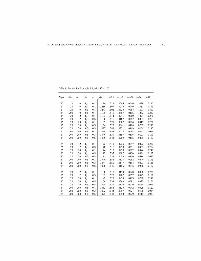
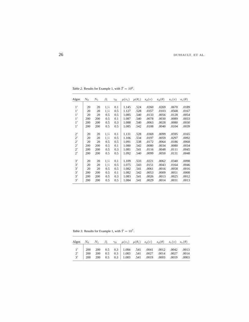
A selection of results is given in Tables 1–3 forT = 105, 106 and107.

From those tables, we can observe the following.

1. WhenNi is fixed to a small constant, the algorithm does not converge to the optimizer.This can be seen by looking at thesd andse values whenN1 = 0: a smallsd and largese indicate a small variance but large bias.

2. All three algorithms appear to converge at the canonical rate ofO(T−1/2); that is, whenT is multiplied by 100,sd andse are roughly divided by 10.

3. For that particular example,βi = 0.5 andMi = Ni = 200 + 200i appear to work well.It other words, it is better in this case to switch not too frequently between SA and SC,and to insure that a large number of regenerative cycles is used at every SC iteration.

Of course, these observations stand only for this particular example; the algorithms canbehave much differently in other situations. Nevertheless, this is a first step towards gettinginsight about what goes on. We certainlycannot saythat these algorithms always work welland are easy to implement in general. Among the difficulties that may arise, we mentionthe following:

1. Implementing the projection onV × Θ when it is a non-rectangular set; and decidingwhat to do if it is non-convex.

2. Choosing appropriate sequences{Mi, Ni, βi, γn} for the problem at hand (the perfor-mance of the algorithm is generally quite sensitive to those choices, and our numericalresults illustrate that to some extent).

3. Choosing the appropriatev0,i and implementing the SC part of the algorithm, especiallyfor Algorithm 3.

More investigation would be required before making specific recommendations for dealingwith those difficulties. Perhaps adaptive heuristic could also be designed. This offerschallenging opportunities for further research.


Table 1.Results for Example 3.1, withT = 105.

Algor. N0 N1 βi γ0 µ(vi) µ(θi) sd(v) sd(θ) se(v) se(θ)

1’ 2 0 1/i 0.1 1.190 .513 .0045 .0046 .1076 .02901’ 20 0 1/i 0.1 1.216 .507 .0078 .0040 .1337 .03411’ 20 0 0.5 0.1 1.241 .502 .0620 .0084 .1691 .04001’ 200 0 0.5 0.1 1.195 .515 .0607 .0115 .1262 .02801’ 20 2 1/i 0.1 1.183 .514 .0211 .0069 .1021 .02761’ 20 2 1/i 0.5 1.180 .516 .0187 .0082 .0993 .02631’ 20 20 1/i 0.1 1.169 .521 .0302 .0084 .0915 .02211’ 20 20 1/i 0.5 1.154 .527 .0341 .0164 .0789 .02101’ 20 20 0.5 0.5 1.097 .542 .0221 .0119 .0254 .01131’ 200 200 0.5 0.1 1.068 .545 .0233 .0068 .0262 .00761’ 200 200 0.5 0.3 1.076 .539 .0197 .0106 .0197 .01031’ 200 200 0.5 0.5 1.076 .542 .0209 .0155 .0209 .0147

2’ 20 2 1/i 0.1 1.172 .519 .0226 .0057 .0922 .02272’ 20 2 1/i 0.5 1.178 .516 .0278 .0091 .0993 .02642’ 20 20 1/i 0.1 1.174 .517 .0238 .0067 .0944 .02492’ 20 20 1/i 0.5 1.115 .535 .0387 .0130 .0494 .01372’ 20 20 0.5 0.5 1.111 .539 .0453 .0100 .0516 .00972’ 200 200 0.5 0.1 1.040 .554 .0127 .0062 .0444 .01432’ 200 200 0.5 0.3 1.044 .550 .0147 .0114 .0407 .01382’ 200 200 0.5 0.5 1.058 .546 .0155 .0095 .0286 .0102

3’ 20 2 1/i 0.1 1.180 .515 .0130 .0040 .0986 .02703’ 20 2 1/i 0.5 1.133 .525 .0207 .0057 .0545 .01673’ 20 20 1/i 0.1 1.149 .523 .0435 .0125 .0790 .02183’ 20 20 1/i 0.5 1.106 .534 .0300 .0081 .0375 .01063’ 20 20 0.5 0.5 1.094 .537 .0120 .0020 .0160 .00433’ 200 200 0.5 0.1 1.052 .553 .0120 .0042 .0325 .01203’ 200 200 0.5 0.3 1.072 .544 .0097 .0021 .0138 .00343’ 200 200 0.5 0.5 1.075 .543 .0093 .0029 .0115 .0035

26 DUSSAULT, ET AL.

Table 2.Results for Example 1, withT = 106.


1’ 20 20 1/i 0.1 1.145 .524 .0260 .0269 .0670 .01891’ 20 20 1/i 0.5 1.127 .528 .0357 .0103 .0568 .01671’ 20 20 0.5 0.5 1.085 .540 .0133 .0056 .0128 .00541’ 200 200 0.5 0.1 1.087 .540 .0078 .0030 .0089 .00331’ 200 200 0.5 0.3 1.088 .540 .0063 .0028 .0080 .00301’ 200 200 0.5 0.5 1.085 .542 .0108 .0040 .0104 .0039

2’ 20 20 1/i 0.1 1.131 .528 .0369 .0099 .0595 .01652’ 20 20 1/i 0.5 1.106 .534 .0197 .0059 .0297 .00922’ 20 20 0.5 0.5 1.091 .538 .0172 .0064 .0186 .00682’ 200 200 0.5 0.1 1.080 .542 .0080 .0034 .0080 .00342’ 200 200 0.5 0.3 1.081 .541 .0116 .0048 .0111 .00452’ 200 200 0.5 0.5 1.092 .540 .0099 .0050 .0131 .0048

3’ 20 20 1/i 0.1 1.109 .533 .0221 .0062 .0340 .00983’ 20 20 1/i 0.5 1.075 .543 .0151 .0043 .0164 .00463’ 20 20 0.5 0.5 1.082 .541 .0061 .0016 .0058 .00163’ 200 200 0.5 0.1 1.082 .542 .0053 .0009 .0051 .00083’ 200 200 0.5 0.3 1.083 .541 .0026 .0013 .0025 .00123’ 200 200 0.5 0.5 1.084 .541 .0029 .0014 .0031 .0013

Table 3.Results for Example 1, withT = 107.


1’ 200 200 0.5 0.3 1.084 .541 .0041 .0012 .0042 .00132’ 200 200 0.5 0.3 1.083 .541 .0027 .0014 .0027 .00143’ 200 200 0.5 0.3 1.083 .541 .0019 .0003 .0019 .0003


Acknowledgments

This work was supported by NSERC-Canada grants no. OGP0110050 and OGP0005491,FCAR-Quebec grant no. EQ2831, and the Technion V.P.R. Fund — B.R.L. BloomfieldIndustrial Management Research Fund. We wish to thank G. Kochman, B. Polyak, andS. Uryas’ev for valuable comments and suggestions.

References

Asmussen, S. and R. Y. Rubinstein (1992a). The efficiency and heavy traffic properties of the score functionmethod for sensitivity analysis of queueing models.Advances in Applied Probability, 24, 172–201.

Asmussen, S. and R. Y. Rubinstein (1992b). Performance Evaluation for the Score Function Method in SensitivityAnalysis and Stochastic Optimization.International Workshop on Computer-Intensive Methods in DiscreteEvent Systems, Vienna, 1990, (G. Pflug ed.). Springer-Verlag, 1–12.

Asmussen, S., R. Y. Rubinstein, and C. Wang (1994). Estimating Rare Events via Likelihood Ratios: From M/M/1Queues to Bottleneck Networks,Journal of Applied Probability, 31, 797–815.

Basar, T. (1987). Relaxation techniques and asynchronous algorithms for on-line computation of non-cooperativeequilibria,Journal of Economic Dynamics and Control, 11, 531–549.

Bertsekas, D. P. and J. N. Tsitsiklis (1989).Parallel and distributed computation: Numerical methods, Prentice-Hall.

Ermoliev, Y. M. (1983). Stochastic Quasigradient Methods and their Application to System Optimization,Stochas-tics, 9, 1–36.

Ermoliev, Y. M. and Gaivoronski, A. A. (1992). Stochastic Quasigradient Methods for Optimization of DiscreteEvent Systems,Annals of Operations Research, 39, 1–39.

Glasserman, P. (1991).Gradient Estimation via Perturbation Analysis, Kluwer Academic Press.Glynn, P. W. and D. L. Iglehart (1989). Importance Sampling for Stochastic Simulations,Management Science,

35, 11, 1367–1392.Glynn, P. W. (1990). Likelihood Ratio Gradient Estimation for Stochastic Systems,Communications of the ACM,

33, 10, 75–84.Glynn, P. W., L’Ecuyer, P., and Adès, M. (1991). Gradient Estimation for Ratios,Proceedings of the 1991 Winter

Simulation Conference, IEEE Press, 986–993.Goldsman, D., Nelson, B., and Schmeiser, B. (1991). Methods for Selecting the best System,Proceedings of the

1991 Winter Simulation Conference, IEEE Press, 177–186.Heidelberger, P., X.-R. Cao, M. A. Zazanis, and R. Suri (1988). “Convergence Properties of Infinitesimal Pertur-

bation Analysis Estimates”,Management Science, 34, 11, 1281–1302.Kleijnen, J. P. C. and Van Groenendaal, W. (1992).Simulation: A Statistical Perspective, Wiley, Chichester.Kushner, H. J. and D. S. Clark (1978).Stochastic Approximation Methods for Constrained and Unconstrained

Systems, Springer-Verlag, Applied Math. Sciences, Vol. 26.Law, A. M. and Kelton, W. D. (1991).Simulation Modeling and Analysis, second edition, McGraw-Hill.L’Ecuyer, P. (1990). A unified view of the IPA, SF, and LR gradient estimation techniques.Management Science,

36, 1364–1384.L’Ecuyer, P. (1992). Convergence rates for steady-state derivative estimator.Annals of Operations Research, 39,

121–136.L’Ecuyer, P. (1993). Two Approaches for Estimating the Gradient in Functional Form,Proceedings of the 1993

Winter Simulation Conference, IEEE Press, 338–346.L’Ecuyer, P. and G. Perron (1994). On the Convergence Rates of IPA and FDC Derivative Estimators.Operations

Research42, 643–656.L’Ecuyer, P. and P. W. Glynn (1994). Stochastic Optimization by Simulation: Convergence Proofs for the GI/G/1

Queue in Steady-State.Management Science40, 1562–1578.L’Ecuyer, P., N. Giroux, and P. W. Glynn (1994). Stochastic Optimization by Simulation: Numerical Experiments

for the M/M/1 Queue in Steady-State.Management Science40, 1245–1261.L’Ecuyer, P. and G. Yin (1994). Budget-Dependent Convergence Rate of Stochastic Approximation. To appear

in SIAM Journal on Optimization.

28 DUSSAULT, ET AL.

Pflug, G. Ch. (1990). On-Line Optimization of Simulated Markov Processes.Mathematics of OperationsResearch15, 381–395.

Pflug, G. Ch. (1992). Gradient Estimates for the Performance of Markov Chains and Discrete Event Processes.Annals of Operations Research39, 173–194.

Plambeck, E. L., Fu, B.-R., Robinson, S. M., and Suri, R. (1993). Optimizing Performance Functions in StochasticSystems. Submitted.

Polyak, B. T. and Juditsky, A. B. (1992). Acceleration of Stochastic Approximation by Averaging,SIAM J. onControl and Optimization30, 4, 838–855.

Reiman, M. I. and A. Weiss (1989). Sensitivity analysis for simulations via likelihood ratios,Operations Research37, 830–844.

Rubinstein, R. Y. (1976). A Monte Carlo method for estimating the gradient in a stochastic network. Unpublishedmanuscript, Technion, Haifa, Israel.

Rubinstein, R. Y. (1986).Monte Carlo Optimization Simulation and Sensitivity of Queueing Network, John Wiley& Sons, Inc., New York.

Rubinstein, R. Y. (1992). Monte Carlo Methods for performance evaluation, sensitivity analysis and optimizationof stochastic systems,Encyclopedia of Computer Science and Technology(Kent ed.), Marcel Deker, Inc., Vol.25, 211–233.

Rubinstein, R. Y. and A. Shapiro (1993).Discrete Event Systems: Sensitivity Analysis and Stochastic Optimizationvia the Score Function Method, John Wiley & Sons.

Rubinstein, R. Y. and S. Uryas’ev (1994). On Relaxation Algorithms in Computation of Non-Cooperative Equi-libria, IEEE Transactions on Automatic Control, AC-39, 6, 1263–1268.

Suri, R. and M. A. Zazanis (1988). Perturbation analysis gives strongly consistent sensitivity estimates for theM/G/1 queue,Management Science, 34, 1, 39–64.

Uryas’ev, S. P. (1992). A Stochastic Quasigradient Algorithm with Variable Metric,Annals of Operations Re-search, 39, 251–267.

Wolff, R. (1989).Stochastic Modeling and the Theory of Queues, Prentice-Hall.Yang, W.-N. and Nelson, B. L. (1991). Using Common Random Numbers and Control Variates in Multiple-

Comparison Procedures,Operations Research, 39, 4, 583–591.