Coherent Marine Radar Measurements of
Ocean Surface Currents and
Directional Wave Spectra
Dennis B Trizna Imaging Science Research, Inc.
6103B Virgo Court
Burke, VA 22015 USA
Abstract- A coherent marine radar with 3-m resolution has
been developed that measures the radial component of the orbital wave velocity of ocean waves, as well as the mean radial ocean surface velocity. This radar allows direct measurement of the ocean wave spectrum by means of 3D-FFT processing of a sequence of coherent radar images of orbital wave patterns. Currently, with a 2.5-s rotation rate, 256 images cover a period of the order of ten minutes, with frequency alias at 0.2 Hz, with upgrade to 0.4 Hz planned with later units. Radial current maps are obtained by a superposition of all radial velocity images collected. This summing forces orbital wave patterns to blend to the mean, resulting in the map of mean radial current. A pair of such radars operated at a coastal site, separated by a few hundred meters along the coastline, may allow the combination of 2-site radial components to be combined into a mean current vector field. Results of first tests of the first prototype radar measurement of radial current and RMS wavehieght are presented for a field site at the U.S. Army Corps of Engineers Field Research Facility, Duck, N.C.
I. OMEGA-K SPECTRA
Marine radar offers a snapshot sequence every 1.25 to 2.5 s
of the coastal wave field that can be used for the application of
a number of image processing algorithms. A number of
researchers have established the utility of using both radar and
optical video image sequences to derive useful coastal ocean
properties from such data [1-6]. We fave recently developed an
integrated radar and data acqusition package to make such
measurements synoptically and unattended. The prototype
system has been set up at the U.S. Army Corps of Engineers
Field Research Facility (FRF), Duck, NC for extensive testing
and ground truth comparison. Real time results can be viewed
at the FRF website (frf.usac.army.mil/radar). The coherent
marine radar processing is very similar to that of the non-
coherent version, as maps of ocean waves are also created.
However, in the case of the standard marine radar, the image is
one of backscatter intensity. For the coherent marine radar, the
image will be the radial component of orbital wave velocity,
that will represent traveling ocean wave orbital wave velocity
maps. As the processing is similar for both cases, we first
present the general approach used for the standard marine radar.
II. COHERENT RADAR DESCRIPTION
Use of non-coherent marine radar for ocean wave spectra
measurement is feasible by making use of multiple-rotation
images, and 3-D FFT image processing to derive Ω-K ocean
wave spectra [1-7]. We have developed a similar capability,
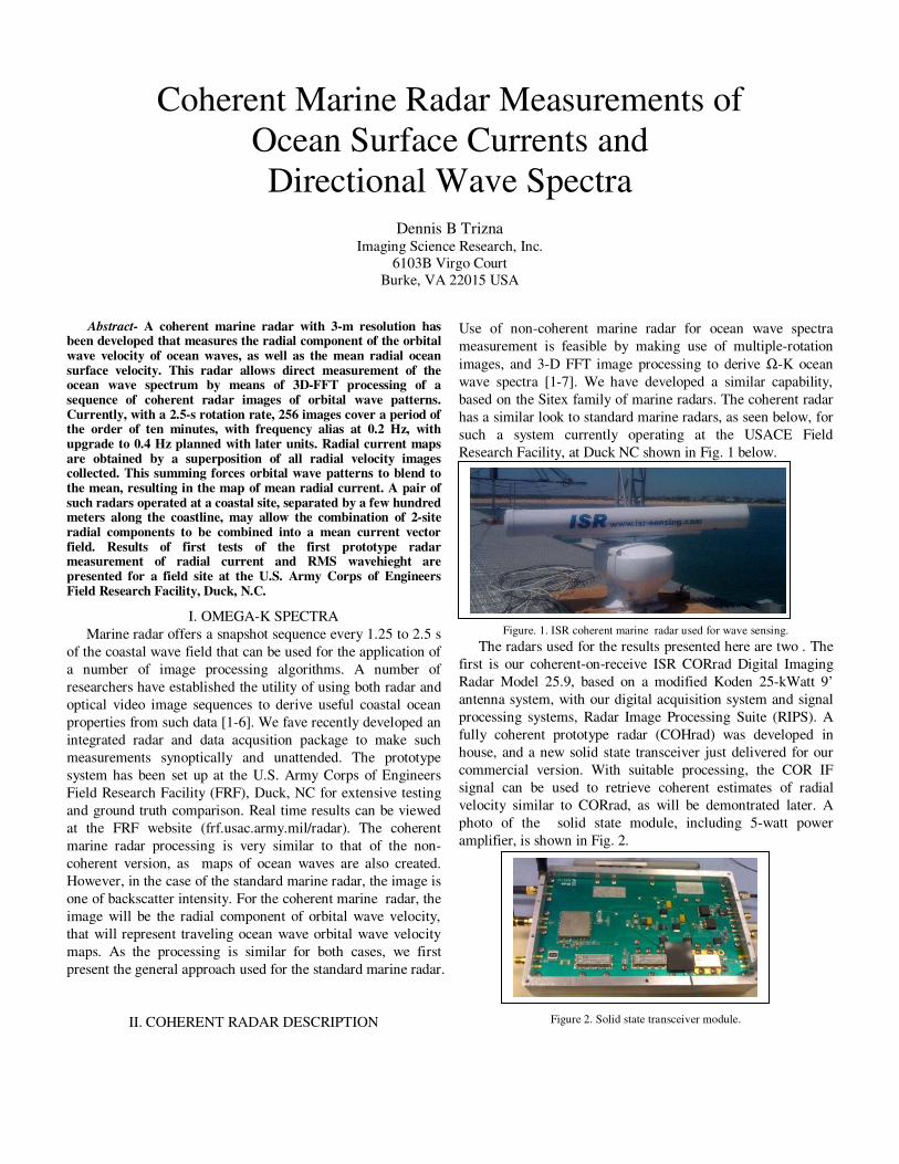
based on the Sitex family of marine radars. The coherent radar
has a similar look to standard marine radars, as seen below, for
such a system currently operating at the USACE Field
Research Facility, at Duck NC shown in Fig. 1 below.
Figure. 1. ISR coherent marine radar used for wave sensing.
The radars used for the results presented here are two . The
first is our coherent-on-receive ISR CORrad Digital Imaging
Radar Model 25.9, based on a modified Koden 25-kWatt 9’
antenna system, with our digital acquisition system and signal
processing systems, Radar Image Processing Suite (RIPS). A
fully coherent prototype radar (COHrad) was developed in
house, and a new solid state transceiver just delivered for our
commercial version. With suitable processing, the COR IF
signal can be used to retrieve coherent estimates of radial
velocity similar to CORrad, as will be demontrated later. A
photo of the solid state module, including 5-watt power
amplifier, is shown in Fig. 2.
Figure 2. Solid state transceiver module.

The radar makes use of pulse compression to achieve
improved gain over the standard marine radar, allowing it to
operate with just 5-watts of peak power. A 1-µs pulse that is
transmitted is shown in Fig. 3a below, chirped over 30 MHz in
this case, and mixed up to X-band for transmission. Echoes
have a similar shape and pulse compression correlation creates
in-phase (I) and quadrature (Q) samples that are used for
velocity measures. These are shown in Fig. 3b and 3c below.
Figure 3a. Chirped pulse transmitted, after mixing to X-band.
Figure 3b. In-phase pulse compressed echo using 3a.
Figure 3c. Quadrature signal (90 deg out of phase with I).
The phase at each time sample is determined from the
equation ATAN(I/Q), and a phase difference, dφ, from two
consecutive pulses is calculated for each range sample. This is
proportional to the radial velocity using the Doppler equation,
v = dφ / (λ/2). The range-azimuth matrix of radial velocities
are then transformed into Cartesian co-ordinates for each
rotation of the radar. The radar video echo intensity signal,
S(R.φ), can be formed at each pixel for comparison using
S(R.φ) = (I2+Q2)1/2. A map of images of intensity and radial
velocity is shown below in Fig. 4a and 4b.
Figure 4a. Radar echo intensity image.
Figure 4b. Radial velocity image.
The radial velocity map appears to show usable information
at ranges where the intensity signal is weak, but stil provides
quality I/Q values to allow phases to be determined. There is
an offset due to current here that will be discussed later. The
red box represents a user-selectable set of pixels that can be
chosen for successive rotations to be used as input to a 3D-FFT
analysis that is used to determined values of spectral samples

of waveheight-squared/Hz. This window can be moved about
the radar coverage scene to study wave dissipation, for
example, or wave refraction spectra in unusual bathymetry
environments. One must correct for the radar aspect relative to
the primary wave direction, as the radar radial component will
vary like cosine of the difference of wave travel vs radar
illumination.
III. OMEGA-K SPECTRA
Fig. 5 represents a subset of frequency spectra from a set of
32 that are available when using 64 rotations of 64x64 pixels,
then averaging over 8 of such sets covering a 10-min period.
The yellow circle seen represents the shallow water dispersion
rule for the depth chosen, 10 m, while the red circle represents
deep water.
Figure. 5. Kx-Ky Spectra at each of a series of wave frequencies from the
Ω-K spectral analysis.
The spectral peaks clearly lie on the shallow water
dispersion circle chosen, and each image can be filtered using a
band between 80% and 120% of this radius, to account for tidal
changes in depth. All energy in this band will represent
samples of wave height squared per unit Hz, (0.4Hz/64 in this
case). This is obtained by relating the radial velocity from the
radar measure to the spectral waveheight component using the
time derivative of the equation defining the x-position of a
patch of water on a wave surface :
X(t) = (H/2) cos(Ωt) (1)
In the case of processing the intensity image of a standard
marine radar, similar image intensity spectra result, but each
radar frequency component must be scaled to some surface
truth representation of the weave frequency spectrum using an
emprical constant, a spectral Modulation Transfer Function.
This has shown to be in error when environental conditions
change (wind direction relative to wave direction, for example),
and if the radar modulator ages with time and exhibits chaning
output power. The coherent radar approach requires no such
scaling, and is independent of such environmental factors. A
patent based on this approach has been applice for by ISR and
is pending, and an international provisional patent has also
been filed.
IV. FREQUENCY SPECTRA AND Hm0
If one sums the spectral energy in the band about the shallow
water dispersion relation for each of 32 windows, one derives
an omni-directional freqeuency spectrum. A comparison of that
derived from coherent radar data over 10 minutes, and the
pressure array sensor at the FRF for two overlapping periods of
3-hr each is shown in Fig. 6 below.
Figure 6. Frequency spectra from COHrad and FTF pressure array.
If one sums the energy from each spectral peak in the
frequency spectrum above, one forms Hm0, a RMS waveheight
estimate. During November of 2009, Hurricane Ida passed
offshore of the FRF site and waves of 4-m were observed.
Below are plotted the time series of Hm0 from the radar vs that
from the FRF pressure sensor array.
Figure 7. Hm0 time series from radar vs FRF pressure array compared.
The black circles represent very short times of collections, just
64 rotations covering ~2.5 minutes, enought for a single 3D-
FFT analysis. As the winds subsided but the waves still being
high, the collections were increased to 256 rotations,
represented by the red circles. The agreement is quite good for
these conditions and illumination into waves offshore of the
pier end. The outlier data might also be due to very large
breaking waves offshore, enhancde using H-pol antenna.

The CORrad was run simultaneously from the same location a
frew meters away and processing that data in a similar fashion
produced results for Hm0 as well. These are shown in Fig. 8
below.
Figure 8. CORrad Hm0 vs FRF pressure array results, with outliers again.
The results from the CORrad system are quite similar to
those of the COHrad for the same period, and outliers for the
higher wave conditions occur here as well.
A third radar was operated at a different time in 2010, from a
location on shore instead of the end of the pier. This is a
scenario that is more likely for most potential applications.
This was data from a CORrad as well, running over 512
rotations at twice the rotation rate of the COHrad, so covering
the same 10-min or so time period. The height of the antenna
was lower than that at the end of the pier, atop a 32’
telescoping tower on ~3-m mean height behind the dune at the
FRF site. They were collected at relatively short range, 384 m
offshore, as onley 512 range samples were collected, and
compared with FRF data from ~800 m offshore.
Figure 9. CORrad data from a shore site.
In this case, the results show the effect of the depth change
with tidal cycle for the higher eave conditions, which was not
accounted for. Nonetheless, the comparison is quite good for
this shore side location.
V. VERTICAL POLARIZATION DURING IRENE
In the summer of 2011, Hurricane Irene passed the Outer
Banks inland of our radar site, but waves generated earlier
while the storm was still offshore generated 4.2 m waves at the
FRF pier. In preparation for this storm, the COHrad antenna
was switched from a 9’ horizontally polarized antenna to a 4’
vertically polarized unit. The hypothesis to explain the outliers
seen in the previous figures was that for very high waves,
severe spilling breakers were occurring in far deeper water
than under lower wave conditions, and the acceleration of
wave breaking crests under such conditions might be biasing
the radial velocity measurements made with horizontal
polarization. In a previous work (Trizna & Carlson, 1996), we
showed the dramatic difference between low grazing angle
images for HH and VV polarization. For HH, small scale
breaking features dominate the scene, with their azimuthal
dependence suggesting a scattering width of about 25 cm, with
virtually no echo when seen from a direction illuminating the
back of these waves, opposite the wind. For VV, these echoes
do not appear, and distributed Bragg sources dominate the
scattering process, with a modest front-to-back ratio of 6 dB or
so when looking into the wind versus opposite it. This suggests
that a vertically polarized antenna might eliminate outliers.
Figure 10 shows a time series of Hm0 measured using
COHrad with the V-pol antenna for wave conditions up to 4.2
m. The outliers that occurred previously are not seen here.
Figure 10. COHrad data during Irene with a V-pol antenna.
For the same time, a CORrad was run with an H-pol antenna,
covering the same period of collection and location at the end
of the FRF pier. There were outliers in these data, starting at
about the same Hm0 value as in the figures above. Thus, we
feel that our hypothesis that outliers for high sea states above
3.5 m or so will generate errors in Hm0 retrieval. However, as
small scale breaking allows one to image the location of the
offshore bar, as we have shown previously, there may be a
trade off in keeping an H-pol antenna for coastal sites, where
the very high sea conditions are rarely encountered, but bard
imaging is important. We have not yet compared the sensitivity
between the two polarizations for very weak wave conditions,
where H-pol might provide a reasonable echo for other
applications as well. The agreement for the 0.4-m minima seen
in Figure 10 do suggest that the ability to retrieve wave
spectral conditions for small waves is not hampered severly.

VI. RADIAL SURFACE CURRENTS
As discussed earlier, if one takes the mean of the sum of all
radial velocity images, in the absence of severe shadowing of
the wave troughs by wave crests for steep wave conditions and
modest to high waves, one can derive radial surface currents
from either type of radar discussed here. Fig. 11 below shows
an example of 256 rotations summed for both radial velocity
and magnitude images for the COHrad system during the Nov
2009 storm.
Figure 1 Summed radial velocity (top) and intenssity (bottom). The gap in
the upper right quadrant of the redial velocity image is due to shadowing of the
radar beam.
The maximum range extent in this case is about 700 m for
the 1.5 km radar coverage (the pier is 600 m offshore). The
drop off in radial velocity is thought to be due to the onset of
shadowing, but has not been investigated thuroughly. Recent
tests using a 19-m radar height was able to image currents out
to 3-km range, so radial current measure is dependent on
antenna height.
As the radar was turned during the experiment, it was
difficult to make comparisons directly over surface truth
currents from bottom mounted acoustic sensors that gave
vector values. Instead, we calculated currents over a range-
azimuth ring, summing between 250-250 meters range extent,
then over 10 adjacent azimuthal bearings of the 595 that were
avialable. The maximum value in azimuth was determined to
be a measure of maximum mean current. The acoustic Doppler
vector currents were used to get a magnitude time history as
well and these were compared. Because the maximum radar
current magnitude was not necessarily at the same range-
azimuth as the 5-m acoustic sensor, nor at the same depth, the
comparisons should be taken with a grain of salt. The results of
such a comparison is shown in Fig. 12.
Figure 12. Time series of COHrad current magnitude (red triangles) and 3
acoustic depths near the surface, with scatter diagram comparison.
VIII. SUMMARY
We have demonstrated the use of a newly designed coherent
marine radar to measure directional wave spectra and surface
radial currents. Data were compared with surface truth
instrumentation from the USACE Field Research Facility, both
pressure array sensor data for wave height, and AWAC
acoustic sensors for currents. Data from a coherent-on-receive
radar that was run simultaneousl from the end of the pier at the
FRF and compared favorably as well. For this location,
currents along shore can be measured reasonably accurately for

the modest radar height of roughly 11 m, as the radar is
looking along the crests and troughs and does not suffer
shadowing, even for modest to low radar height for this
geometry. Looking offshore, the troughs would be shadowed
by the crests for very steep waves, and the orbital wave
velocity would not present a zero mean to the radar look. We
found this to be the case for a shore based radar on another
occasion, where the currents were in error due to crest orbital
wave influences. For this case, the wave height analysis was
still quite respectable. On more recent observations at other
sites with radar heights ranging from 19 m to 26 m, no
shadowing was encountered and long range currents could be
measured accurately.
A pair of radars discussed here, placed of the order of 300 to
1,000 m apart, should be able to provide a vector map of
surface currents at 3-m resolution. Such a method should be
useful for detection of rip currents and riverene flow, in
addition to currents in harbors for ship traffic application.
ACKNOLEDGEMENTS
We wish to acknowledge the data provided by the USACE
FRF, in particular, to Kent Hathaway who extracted the data
from historical records that allowed the comparisons to be
made on a timely basis. ISR has a continuing Co-operative
R&D Agreement with the FRF.
The processing and analysis involved in generating results
such as that shown here have patent applications currently
pending in the U.S., Canada, and the European Union.
REFERENCES
[1] H. Dankert J. Horstmann, and W. Rosenthal, Ocean Wind Fields
Retrieved from Radar-Image Sequences, J. Geophys. Res.. Vol. 108, 2005.
[2] I.R.Young, , W. Rosenthal, F. Ziemer, A three-dimensional analysis of marine radar images for the determination of ocean wave directionality and
surface currents, JGR, 90, C1, pp. 1049-1059, 1985. [3] D.B. Trizna, “Errors in Bathymetric Retrievals using Linear Dispersion
In 3D FFT Analysis of Marine Radar Ocean Wave Imagery,” IEEE
Trans. Geosciences and Remote Sensing, 39, pp. 2465-2469, 2001.
[4] C.M. Senet, J. Seemann, F. Ziemer, An iterative technique to determine the near surface current velocity from time series of sea surface images, Oceans ’97, Halifax, 1997.
[5] Dugan, J.P., H.H. Suzukawa, C.P. Forsythe, M.S. Farber, Ocean wave dispersions surface measured with airborne IR imaging system, IEEE Trans. Geosciences and Remote Sensing, 34, pp. 1282-1284, 1996.
[6] Dugan, J.P., C.P. Forsythe, H.H. Suzukawa, M.S. Farber, Bathymetry estimates from long range airborne imaging systems, Proc. 4th Int. Conf. On Remote Sensing for Marine and Coastal Environments, Orlando FL, 1997.
[7] Stockdon, H.F., and R.A. Holman, Estimation of wave phase speed and nearshore bathymetry from video imagery, J. Geophysical Res., 105, pp. 22,015-22,034, 2000.
[8] McGregor, J.A., E.M Poulter, M.J. Smith, Switching system for single antenna operation of an S-band FMCW radar, IEE Proc. –Radar, Sonar, Navig, Vol. 141, pp 241-248, 1994.
[9] Trizna, D.B., and D. Carlson, Studies of low grazing angle radar
seascatter in nearshore regions, IEEE Trans. Geosciences and Remote
Sensing, 34, pp. 747-757, 1996.
Recommended